OSSCAR, an open platform for collaborative development of computational tools for education in science

Abstract

In this paper we present the Open Software Services for Classrooms and Research (OSSCAR) platform. OSSCAR provides an open collaborative environment to develop, deploy and access educational resources in the form of web applications. To minimize efforts in the creation and use of new educational material, it combines software tools that have emerged as standards with custom domain-specific ones. The technical solutions adopted to create and distribute content are described and motivated on the basis of reliability, sustainability, ease of uptake and use. Examples from courses in the domains of physics, chemistry, and materials science are shown to demonstrate the style and level of interactivity of typical applications. The tools presented are easy to use, and create a uniform and open environment exploitable by a large community of teachers, students, and researchers with the goal of facilitating learning and avoiding, when possible, duplication of efforts in creating teaching material. Contributions to expand the educational content of the OSSCAR project are welcome.

1 Introduction

Software-based tools, such as notebooks or illustrative codes, are increasingly employed in scientific courses to enrich and complement more standard teaching approaches. These tools can provide an interactive environment for teachers to demonstrate, via live examples and engaging visualization, complex and abstract concepts that may otherwise be difficult to transmit. At the same time, students can gain intuition, facilitate understanding and strengthen learning [1] by exploiting them as simple virtual laboratories, e.g., to experiment in real time with the effect of relevant parameters in equations. Given these advantages, and with the growing relevance of remote education, software-based educational tools are becoming more common. For example, Quantum Physics Online [2] publishes online Java applets with visualizations that illustrate topics typically covered in undergraduate and master level courses in that area. Considering more domain-specific examples, the Soft Matter Demos [3] or NanoHub [4] websites present simulations and visualizations to stimulate interest in these domains, with a limited interest in coursework. Other open-source platforms offer visual tools for education in chemistry in the form of interactive simulations [5]. Use of e-tools based on Google Colab was recently explored [6] to support the teaching of thermodynamics and provide some introduction to coding in chemistry classes taught in Columbia. Further impetus to develop on-line teaching tools was added by the recent pandemic crisis [7, 8, 9], with several interesting studies on their effectiveness [10, 11, 12].

In spite of their great potential, widespread adoption and sharing of software-based tools for teaching is, however, still hindered by different barriers. On the side of the teachers, the time investment to create bespoke material for different classes might be considerable and efforts frustrated by the lack of agile development and deployment environments. Moreover, curating the material to counteract software obsolescence, guaranteeing resilience to changes in versioning of the adopted language, and facilitating updates when content evolves are all non-trivial challenges. Furthermore, given that the same type of material is needed for classes across different areas and in different institutions, the risk of effort duplication is very high. No “public library” of software teaching tools exists to reduce this risk and limit the teachers’ effort only to the creation of new, original material. On the side of the students, uptake and usage of these tools can be problematic depending on the technology employed to deploy them and the level of user-friendliness of the platforms to access them. Also, the lack of a coherent platform may force them to spend considerable effort to migrate from one technological solution to another when changing class.

In this paper, a new platform that attempts to overcome these barriers is presented: the Open Software Services for Classrooms and Research (OSSCAR). OSSCAR is inspired by the software architecture developed as part of AiiDAlab [13], a platform designed to provide easy access to research-oriented software, workflows and tools via a web interface. OSSCAR adapts and applies these concepts and technologies for education purposes. Specifically, as detailed in Sec. 3, OSSCAR combines and builds upon a set of well-established software tools to create a web-based collaborative environment targeted at providing educational resources and enhancing awareness and adoption of best practices in Open Science. The programming language chosen is Python, and we use Jupyter [14, 15, 16] and JupyterLab [17] as the programming interface and environment. Within this framework, common visualization tools and widgets are employed (and new ones are developed) to create interactive notebooks illustrating specific topics or proposing exercises. Jupyter notebooks are then automatically converted into web applications exploiting the Voila program [18]. The web applications hide all code and show only the outputs (including, in particular, the widgets to interact with the application) in a user-friendly format accessible through any browser, circumventing the need for specific software installation and set up.

The contributions of OSSCAR are along three main lines, detailed in the rest of the paper, and that we summarize here: 1) provide custom graphical components (widgets) for domain-specific visualization types (see Sec. 3.2); 2) provide custom educational content tailored for a number of courses in the fields of computational physics, chemistry and materials science; these are developed in the form of self-contained modules that can be combined and reused also beyond the courses for which they were originally developed (see Sec. 6); 3) provide clear documentation (on http://www.osscar.org), transferring know-how gathered in the past years on how to combine various open technologies to easily develop new educational applications (see Sec. 7) and open to input and feedback from the community.

In the following, we first demonstrate the appearance and structure of an OSSCAR notebook via the example of a classic problem in quantum mechanics: the double-well potential. We then provide technical details on the tools employed to develop new notebooks and justify our choices. Next, we show some selected examples, based on notebooks developed for Master-level courses in Physics, Chemistry and Materials Science. These examples, all related to quantum-mechanical problems, also suggest that OSSCAR notebooks can act as modules to be combined in various ways for different classes.

While technologically mature, OSSCAR is at the early stages of development in terms of content. It is intended as an open repository to be built in collaboration with the community of students and teachers in scientific disciplines, and we invite contributions from interested groups.

2 An OSSCAR interactive web application example: a quantum-mechanical double-well potential

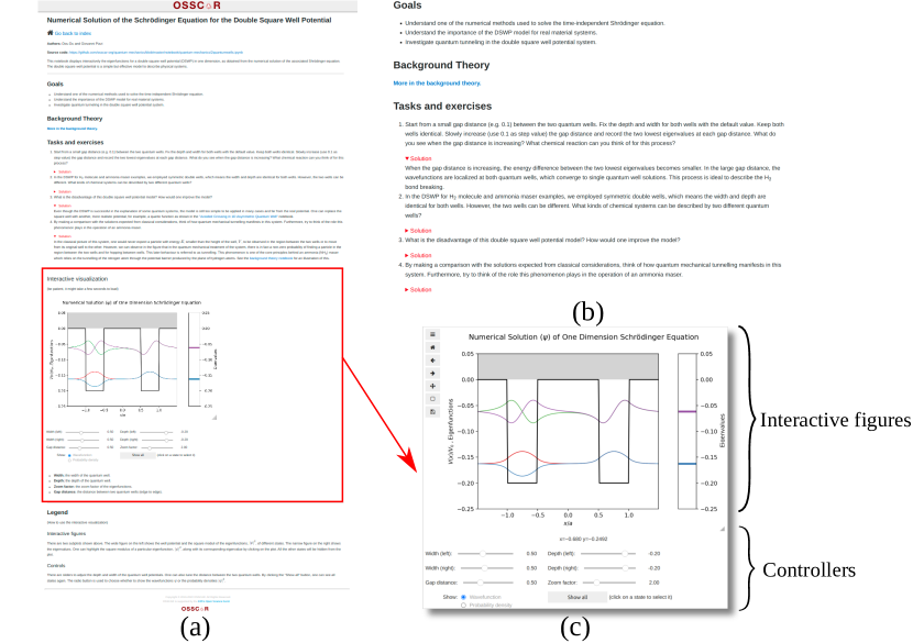
Figure 1: The interactive web application to demonstrate the numerical solution of the Schrödinger equation for a 1D double square-well potential. The web application is hosted at https://osscar-quantum-mechanics.materialscloud.io. a) The whole webpage, showing the typical structure of an OSSCAR notebook: introductory text (zoomed in panel b) including a link to the background theory, the goals of the notebook and a set of tasks and exercises for the students, followed by the interactive visualization (better displayed in panel c), and a legend.

In this section, we discuss a prototypical OSSCAR application: the interactive visualization of the eigenvalues and eigenvectors obtained by solving the one-dimensional (1D) Schrödinger equation for a double square-well potential [19]. To provide a general overview of a typical application, we mainly focus on the key components that are shared among the OSSCAR notebooks, rather than on the specific content of this example. Note that, since the web applications are implemented as Jupyter notebooks, as mentioned in the Introduction and described in more detail in Sec. 3, in the following we will use the terms notebooks and applications (almost) interchangeably.

To clarify the reasons behind the overall structure and graphical appearance of the application, we start by discussing how we expect these notebooks to be employed by teachers and students. In our experience, there are two main use cases, that we shall call A and B. In use case A, the notebooks are used for independent learning by students. Students might have simply found the application online, or might have been referred to it with a web link, for example in a class. In this case, before they are presented with the interactive visualization itself, it is important to provide users with a short explanation of the goals of the application and with some guidance on how to best interact with it to achieve the learning objectives.

In use case B, instead, teachers might use the applications for live demonstrations during their classes to complement and enrich standard lecturing (textbooks, blackboard, slides, …) thus improving students’ learning effectiveness [20]. We include in use case B also the case of teaching assistants that present the notebook content as part of their discussion sessions, because the requirements are relatively similar. In this second scenario, the introductory part of a notebook is not relevant, since the topic has already been introduced and discussed by the teachers, who will instead focus on using the interactive part. In this case, it is essential that applications can be accessed very rapidly (in a matter of seconds), because they will be used only for the minimal time required to convey the message (typically no more than a couple of minutes), before the teachers continue with their lectures. (The students might also use the applications after the lecture is ended to revise the course content, falling back into use case A.)

With these two use cases in mind, we now discuss the structure of a typical OSSCAR notebook, as illustrated in Fig. 1. Each application starts with a brief textual section that we see at the top of Fig. 1(a), including a short list of educational goals, a link to additional background theory, as well as a list of tasks to guide the exploration of the interactive part of the notebook. Authorship is also acknowledged at the top of each notebook to give due credit to contributors and encourage collaborative contributions by other teachers and also by students. This first section addresses the needs of use case A, to quickly assess if the notebook covers the topics of interest and to provide guidance for interacting with the application via a set of tasks for the students. At the same time, this section is kept to a minimum to cover the needs of use case B (or of students already familiar with the application): being short, the section is easy to skip, so one can jump directly to the interactive visualization. In particular, the background theory is discussed in a different, linked, page (and also there only as a brief overview of the physical problem, favoring links to existing online material to avoid content duplication). Furthermore, the solutions for the students’ tasks are hidden by default. This latter design choice not only keeps the first textual section short, but also encourages students to answer the questions themselves rather than read directly the solutions, promoting active learning and thus improving learning effectiveness [21, 22].

Below this textual introduction, we find the interactive visualization section, better displayed in Fig. 1(b). This is the core of the web application. Each interactive visualization is composed of two main groups of components: the interactive figures and the controllers. The controllers are “widgets” (discussed in more detail in Sec. 3.2) such as sliders, dropdown menus, checkboxes or buttons, that allow one to tune some parameters of the model or the visualization itself and whose effect is dynamically reflected in the interactive figures.

In this specific example, the top part with the figures displays the potential energy (thick black line, formed by two square wells) and the wavefunctions (colored thin lines) at the height of the corresponding eigenvalues. The right part of the plot displays the eigenvalues only, represented as thick horizontal lines (with the same color of the corresponding wavefunctions).

In the controllers section of this figure, five sliders are used to tune the width and depth of the two square wells and the distance between the two. Two radio buttons allow the students to decide whether to display the wavefunction $\psi(x)$ or the probability density $|\psi(x)|^{2}$. A sixth slider can be used to determine the “zoom factor” of the wavefunctions (i.e., the multiplicative factor in front of the wavefunction, that is only used to have a nice visualization but does not affect the simulation).

In typical notebooks the figures, in addition to being dynamic (i.e., changing their content as soon as the value of one of the controllers is modified), can also be interactive: for instance, in this specific example, a click on one of the wavefunctions (or on the corresponding eigenvalue on the right-hand side) displays its plot and numerical value, while hiding all other wavefunctions. A button “Show all” in the controllers section allows one to display again all the wavefunctions.

Finally, at the bottom of the page (see Fig. 1(a)), there is a legend that describes in more detail the figure components and the functionality of each controller. This is placed at the bottom of the page as a useful reference, mostly to cover the needs of use case A, but we strive to design the interactive visualizations so that all figures and controls are as intuitive and self-explanatory as possible, reducing to a minimum the need to read the legend.

A collection of OSSCAR web applications can be considered as a “living book”, with powerful interaction and visualization capabilities that go beyond what is achievable on printed text or static images, and can convey more effectively advanced content to students, facilitating their understanding. In addition, the tasks presented at the top of the notebook help students to focus their attention on core concepts. For instance, one of the tasks of this notebook suggests investigating the phenomenon of quantum tunneling and anticrossing of states as a function of the distance between the two wells: by moving the slider to alter the gap distance, students can vividly observe in real time how the wavefunctions and their energies change, something that would be difficult to achieve through traditional teaching.

Finally, at the very top of each page, we also provide a link to the source code of the notebook. We discuss the additional advantages of providing immediate access to the notebook source code in Sec. 7.

3 Technology to develop interactive web applications

One of our key design goals for OSSCAR is to make it simple enough for teachers with basic coding experience to develop further applications. Consequently, as mentioned in the Introduction, the majority of the software stack is deliberately composed of existing open, well documented and well maintained software. The motivation behind doing this is to maximize the lifetime and accessibility of the notebooks by ensuring that they do not depend on custom software and technology that might become unsupported soon. Let us now detail the core technological components of the OSSCAR platform.

3.1 Development environment: Python and Jupyter/JupyterLab

We choose Python as the programming language for the interactive notebooks. Python is a common programming language for data science and scientific computing that has gained popularity in the past years in many computational scientific disciplines [23]. This is probably due to both Python’s syntax, which is relatively easy to learn and quite readable even for people with little programming experience, and to the very large number of free Python packages that can be easily installed via, e.g., the pip [24] or conda [25] package management tools.

Python allows for relatively rapid development, even if (being an interpreted language) it might be slow for expensive computations. The need for performant simulations is less of an issue for education-oriented applications than for scientific production runs, since the main goal is not to obtain results with ultimate precision and speed, but rather to demonstrate the simplest approximation that captures the essential aspects of the model (so that students can focus on the core concepts, and not on the numerical optimizations). In spite of this, in both use cases described in Sec. 2 it is very important that simulations can be performed almost in real time (or in any case, in a matter of seconds). Indeed, in use case A students might easily lose focus if they have to click a button and wait for minutes before the results appear. Moreover, slow execution time limits the interactive capabilities of the applications and the number of different input parameters that students can experiment with. Similarly, teachers in use case B need to be able to demonstrate rapidly the relevant results to students before continuing with their lectures.

While in our experience Python is often fast enough, there are cases in OSSCAR where strategies to speed up the simulations are required (e.g., when performing simulations with millions of iterations, or when dealing with large matrices). We list some of these strategies in A.

For the purpose of creating interactive visualizations, however, the programming language itself is not sufficient, but one also needs a library to enable powerful displays of the results via a graphical user interface (GUI). A relatively large number of GUI libraries are available for Python. Our choice is to use Jupyter notebooks (using a “classic” Jupyter server, or the more recent JupyterLab environment), that provide a notebook interface to interact with Python code. Jupyter has very rapidly gained popularity, also in the scientific context [26, 27] (including for teaching [28]), as a very powerful approach to distribute understandable and reusable code.

Having a notebook interface means that the whole code is divided in cells, and each cell contains only a part of the code that can be executed independently, and whose output is displayed underneath the cell. The advantage is that the notebooks do not contain only the source code, but can also include contextual rich-text annotations, descriptions, and widgets (such as plots, buttons, …– see discussion in Sec. 3.2), combining in a single consistent document both the code and its documentation and visualization.

One of the reasons why we choose Jupyter in OSSCAR, besides its popularity (and thus availability of visualization and widget libraries), is that the GUI is web-based and displays directly in the web browser. As such, it works on any computer operating system (OS) and does not require additional installation of custom software, contrary to typical GUIs that might require one to install OS-specific code and libraries. Having a simple web-based interface is one of the key requirements in OSSCAR to make the use of the applications straightforward. We discuss in the next sections how to implement interactive visualizations within Jupyter notebooks, and then discuss in Sec. 4 how to completely hide the Python code and provide students with a very simple and intuitive web interface.

3.2 Widgets: components for interaction

Visualization plays a crucial role in human learning [29]. This is important, for instance, when dealing with multi-dimensional representations, where interactive 3D plots can be very effective in representing datasets. In particular, in fields such as computational physics, interactive figures can greatly facilitate explanation of abstract concepts compared to text, bare equations or static figures. In B we discuss some plotting libraries for 2D and 3D plots that we use in OSSCAR, with some minimal usage examples.

However, while plots are essential to display the results of a simulation or the values of a function, one additional type of component is crucial to enable interactivity and decide the relevant parameters in the controller section (e.g., the width or depth of the quantum well in the example of Fig. 1). As previously mentioned, these components are called widgets and allow the user both to supply inputs and to trigger events (e.g., via a click on a button). The Python library ipywidgets provides a large number of common native widgets working within Jupyter notebooks, such as sliders, checkboxes, dropdowns, text areas and buttons.

We show in C a simple example, both to illustrate how easy the code to interact with these widgets can be, and to discuss how one can implement instantaneous reaction to events.

3.2.1 OSSCAR custom widgets

When Jupyter-ready widgets are not already available, OSSCAR develops bespoke widgets customized for specific needs, embedded in our applications and realized as open source. A typical example are custom visualizations necessary to display domain-specific content, especially for 3D visualization. While general-purpose 3D libraries exist, they often require one to define the data to visualize at a very low level (e.g. by providing the coordinates of the triangles composing a surface mesh). This is however very cumbersome and requires lengthy custom code, while a teacher would strongly benefit from a simple domain-specific widget requiring only minimal input. Widgets with this goal are provided by OSSCAR as shown in the two examples in Fig. 2. Panel (a) shows a widget to plot the isosurfaces of molecular orbitals [19]. It leverages the NGLview visualizer [30], but exposes a simpler interface to directly plot volumetric data associated to molecules. Panel (b), instead, shows a custom widget to compute and display interactively the first Brillouin zone (BZ) [19] of a crystal. It is based on the JavaScript visualizer developed as part of the SeeK-path library [31], and it exposes to teachers a very simple Python interface: one just needs to provide the three real-space lattice vectors to generate the BZ, where high-symmetry points are automatically displayed and labelled, together with the suggested path to compute band structures. Another example of a custom widget developed in OSSCAR, not shown here, is an interactive periodic table that allows users to select multiple chemical elements (with each of them being in one of a range of possible states, e.g., to select elements to be either included or excluded for searches and filtering).

We emphasize that developing a new widget might not be straightforward, as it requires relatively advanced knowledge of both Python and JavaScript, as well as experience with specific frameworks and libraries in the two languages. However, once a Jupyter widget has been developed and published, its use is very straightforward, typically requiring only a couple of lines of Python code. Therefore, the custom OSSCAR widgets are a powerful catalyst that we provide to facilitate and promote the creation of interactive notebooks with powerful visualizations, and we expect to keep developing new ones with input and contributions from the more expert user community.

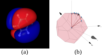
Figure 2: (a) A custom OSSCAR widget to display the molecular orbitals of a molecule (in this example, benzene), wrapping the NGLView Jupyter widget. (b) A custom OSSCAR widget to compute and plot the first BZ of any crystal, together with the labels of high-symmetry points and a suggested path to compute a band structure.

4 Convert notebooks into web applications

In the use cases A and B described in Sec. 2, the primary goal of the interactive visualizations is to deliver physics knowledge, with less emphasis on programming and algorithms behind the notebook. The code might actually be distracting the first time a student interacts with the application, and therefore we prefer to hide it in order to retain clarity in the presentation.

A number of tools have been developed to convert Jupyter notebooks into shareable web applications, including appyters [32], nbinteract [33], bokeh [34], Voila [18], and appmode [35]. In OSSCAR we opted to use Voila, a subproject of Project Jupyter that can turn Jupyter notebooks into live standalone web applications, by executing the whole notebook and rendering only the output cells into a web page format, while all of the source code is hidden. For instance, Fig. 1 shows the page obtained for the double quantum well after rendering the notebook with Voila. Additionally, Voila keeps the Python code active (i.e., an active connection is maintained between the web frontend and the so-called “Python kernel” in Jupyter). This is crucial to allow the Python callbacks (see, e.g., Fig. 8) to be executed when the users interact with the widgets. Other solutions, instead, convert the notebook into a static webpage [36, 37]. While this approach has the advantages of easier deployment (see also Sec. 5), it limits the interaction possibilities. In addition, Voila supports the development of custom templates to modify the overall appearance of web applications. In OSSCAR, we have developed our own template that is also shown in Fig. 1 (e.g., the header and footer with the OSSCAR logo are part of this template) to provide a uniform and consistent look and feel for all notebooks.

While the code can be completely hidden from the user and thus made fully private using Voila, we stress that in OSSCAR we strive to provide a solution that fully complies with the Open Science principles: not only regarding open availability of the applications for reuse in other classes, but also releasing open source all code for inspection and reuse. Therefore, all source code of the OSSCAR notebooks is available as open source on GitHub, and each notebook displays a link to it at the top of each page (see also Sec. 7).

5 Deployment on web/cloud servers

The final aspect of making the notebooks available to a broad audience is their deployment. This is crucial, as most users will not have the time (nor, often, the expertise) to install locally Python, Jupyter and all the dependencies to run the notebooks. Therefore, easy access to the applications with just a web link becomes essential to make them straightforward to use.

However, deployment (especially if it has to be efficient) often comes with some costs associated to it. For instance, hosting content on most public cloud services is not free, while self-hosted servers might also have a non-negligible cost associated to the human time needed to maintain the service (perform system security updates, recover after system crashes, …). Therefore, in OSSCAR we have investigated various solutions and, while we did not find a single one that covers all requirements, we identify, use and suggest three different (free) solutions to deploy and deliver the web applications, depending on the student and teacher needs. These are briefly described below, highlighting pros and cons of each solution.

5.1 mybinder.org

mybinder.org is a website offering a free cloud solution to deploy Jupyter notebooks, and has been already used to serve course content to students [38]. mybinder.org allows one to generate a unique URL associated to a GitHub repository that contains notebooks and code. When a user opens the link, mybinder.org automatically fetches the code and runs it in an isolated environment for each user (using Docker [39] containers behind the scene) so that each user does not interact with others using the application at the same time.

mybinder.org requires minimal effort for teachers. One first has to create a public GitHub repository with the notebooks and some basic configuration files that, as detailed in their documentation, primarily consist of a list of Python dependencies that need to be installed in order to make the notebooks functional. Then, on the mybinder.org homepage, one can easily obtain a unique link (that can be distributed to students, or published on a webpage) to access the deployed application. The link can be obtained simply by providing the GitHub repository name, the Git branch name and the notebook URL (see Fig. 3). Furthermore, using Voila together with mybinder.org is very straightforward: one can just declare Voila among the dependencies, and then prepend the string /voila/render/ to the notebook URL to trigger the Voila extension at load time.

Being free, open and requiring almost zero maintenance effort, this service is extremely useful, but there are two shortcomings. The most critical one is that every time that the page is loaded, the initialization might take a significant amount of time (from a few tens of seconds to some minutes). This might be problematic for the needs of the two use cases described in Sec. 2, and in particular for use case B, where a teacher might want to use the application only for a very short amount of time. In addition, being a free service, the computing power is also very limited, which can be an issue for sophisticated notebooks performing advanced simulations. Nevertheless, we strongly encourage any teacher developing a notebook to provide a mybinder.org link in their homepage, as this makes the notebooks immediately accessible (even if with a lag of a few tens of seconds) to any web user, without any setup needed.

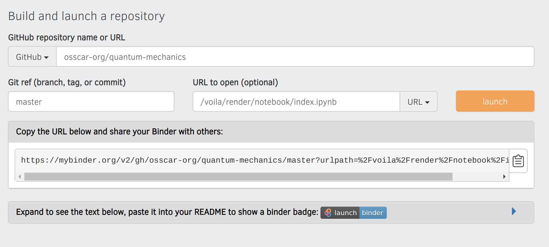
Figure 3: Input GitHub details to generate the mybinder.org link.

5.2 dokku deployment

In order to speed up the startup time of each notebook, we also deploy the OSSCAR notebooks on custom resources using an open-source software called dokku [40]. dokku is an extensible Platform-as-a-Service software that makes deployment of applications extremely easy. In particular, one just needs to place all their code and notebooks inside a Git repository, and push the content to the dokku server to update the deployed version.

Similarly to mybinder.org, dokku transparently creates a Docker container. This container is, however, the same one for all users and user isolation is obtained thanks to Voila. This requires special care when implementing the notebooks to avoid unexpected interactions between users, e.g., if files with the same name are generated on the server. The startup time, however, is considerably reduced, typically to 5 seconds or less.

Unfortunately, this solution also has some shortcomings. In addition to having to understand the deployment model to prevent unexpected interaction among different users, installing and maintaining a dokku server requires the availability of an online server (that might not be free) and most importantly it requires expertise in managing and deploying web servers. In our case, we leverage the dokku service provided by the Materials Cloud portal [41], with servers hosted at the Swiss National Supercomputing Center (CSCS), that kindly provides the resources to host the OSSCAR applications. For instance, the applications for quantum mechanics described later in Sec. 6 can be accessed at the address https://osscar-quantum-mechanics.materialscloud.io. If, however, a teacher does not have access to such a deployment, this solution might not be viable (we note, however, that similar hosted commercial solutions exist, such as heroku.com for instance, that might have a free tier for small non-commercial applications).

5.3 Institutional JupyterHub servers

Because of the widespread adoption of Jupyter, many universities, research centers and computer centres are now offering to their users (teachers, students, researchers) access to locally hosted JupyterHub installations. JupyterHub is an open server facilitating the provision of multi-user access to notebooks.

This solution could be ideal for courses given at universities where this service exists and all students have access to it. The added benefit of this deployment approach is that each student has access to their persistent home folder, where they can not only install and use the applications, but also easily modify the code and run the modified versions, possibly contributing back their changes to the original repository. This solution is therefore particularly suitable if the teachers want to encourage the students to modify and adapt the code of the notebooks.

One example of such an institutional JupyterHub is the NOTO platform at EPFL (https://noto.epfl.ch). We show how a notebook appears inside the JupyterLab interface provided by NOTO in Fig. 4, but we stress that many more universities are already providing a similar service, also thanks to the fact that JupyterHub and JupyterLab are open source and officially supported as part of Project Jupyter.

We finally mention that in terms of use cases covered, also Google Colab [42] can be considered to fall within this category, where rather than institutional credentials one would need instead a Google login.

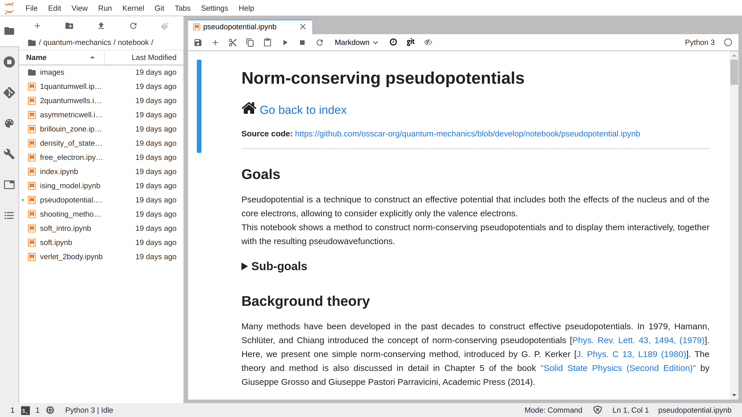
Figure 4: An example of how an OSSCAR notebook is displayed in the JupyterLab interface, in this specific example available via the EPFL NOTO platform.

6 OSSCAR notebooks for computational science

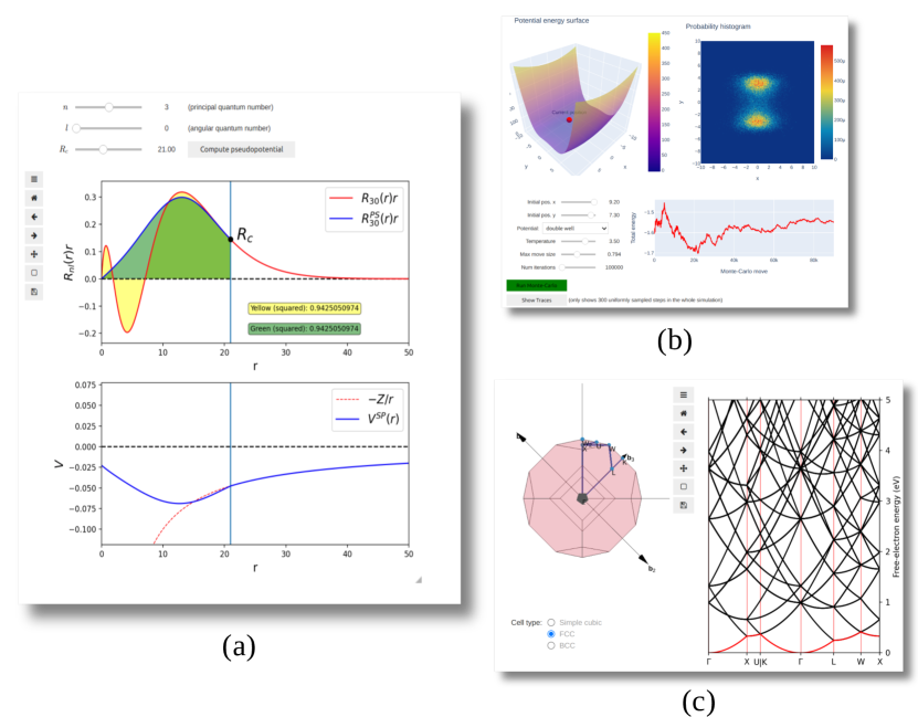
Figure 5: Three interactive web applications developed in OSSCAR and used to complement teaching in classes of computational simulations. The web applications are hosted at https://osscar-quantum-mechanics.materialscloud.io. a) Construction of a norm-conserving pseudopotential. b) Monte-Carlo simulations to sample the canonical distribution of a given potential energy surface. c) Electronic band structure and first BZ of an empty-lattice free-electron crystal.

In addition to proposing guidelines for best practices in developing open teaching content, and developing custom widgets for computational-science content, one of the main goals in OSSCAR is to generate open and free learning content in the broad domain of computational physics, chemistry, and materials science.

OSSCAR currently offers a number of interactive notebooks covering the topics of quantum mechanics, band theory of crystals, statistical mechanics, and molecular dynamics. The choice of the topics stems primarily from the content of two courses taught by some of the authors at EPFL (“Computational methods in molecular quantum mechanics” and “Atomistic and quantum simulations of materials”). The notebooks have been already used in the past year with very positive feedback from students. In particular, anonymous surveys were conducted at the end of one of the courses. The results indicate that for the majority of students (over 70%) the inclusion of interactive visualizations during the classes was both motivating, and helped them to better understand the core course concepts by being actively engaged in the learning process. Furthermore, the same proportion of students also accessed and used the interactive visualizations to improve their understanding after the lectures, while revising the course content (use case A in Sec. 2). Students also provided valuable feedback for improvement of the notebooks, and, in both classes, some even demonstrated interest in generating new educational content using the same OSSCAR approach.

Without aiming at presenting an exhaustive list, in the following we briefly show some selected examples of applications developed in OSSCAR, to demonstrate with practical examples the general concepts and technologies (such as the widgets) described earlier. More applications are available online, and we expect the list to continue growing in the future. The source codes of all notebooks are available on the GitHub repository at https://github.com/osscar-org/quantum-mechanics and can be directly inspected on our dokku server at https://osscar-quantum-mechanics.materialscloud.io.

Fig. 5 presents three different OSSCAR notebooks. As mentioned in B, we use matplotlib to render 2D interactive figures. This is the case, for instance, for the two plots in Fig. 5(a), an application illustrating the construction of norm-conserving pseudopotentials [19]. The two panels display the hydrogen-atom potential and the pseudopotential that was generated (bottom panel) and one of the wavefunctions and the corresponding pseudo-wavefunction (top panel). Users can select the principal quantum number $n$ and the angular quantum number $l$ of the wavefunction in the controllers region, as well as the cutoff radius $R_{c}$ determining the core region.

In Fig. 5(b) we instead show an application that illustrates the use of Monte-Carlo simulations with the Metropolis–Hastings algorithm [43, 44] to sample the canonical distribution at a given temperature $T$ for a potential that can be selected among various possibilities (a 2D double-well potential is selected and shown in the figure). Students can set the starting coordinates $(x,y)$ of the simulation, select the temperature $T$, and tune the simulation parameters (maximum move size and total number of iterations), to investigate both physical (temperature and potential-barrier height) and numerical effects on the efficiency and ergodicity of the simulation. This application displays various types of figures: a 3D visualization of the potential energy surface (top left, displayed with plotly as discussed in B), the probability histogram as a color map obtained from the simulation (top right, displayed using matplotlib), and the total energy as a function of the Monte-Carlo move (bottom right). This notebook is also an example of the Multiple Representation Principle, where complementary representations of related quantities are displayed to facilitate learning, thanks to the different informational content of each of them [45].

Finally, Fig. 5(c) shows an application to compute and show the band structure and BZ of a simple empty-lattice free-electron crystal (for simple, face-centered and body-centered cubic lattices) [19]. The notebook can be used to explain the concept of reciprocal space, discuss how band structure paths are selected, and compare band structures of actual materials with the free-electron case. While the band structure plot (on the right) uses the same matplotlib library that we employ for 2D plots, the left part uses the custom OSSCAR BZ visualizer already described in Fig. 2(b).

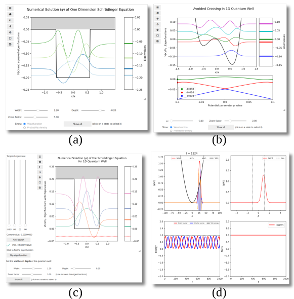
Figure 6: Four OSSCAR applications of different levels (from basic to advanced) addressing the general topic of the solution of the Schrödinger equation, to demonstrate how an advanced topic can be split into smaller self-contained notebooks. a) Numerical solution of the 1D time-independent Schrödinger equation for a single quantum-well potential. b) Avoided crossing in a 1D asymmetric quantum well. c) Explanation of the shooting method and Numerov algorithm to solve the Schrödinger equation. d) Numerical solution of the 1D time-dependent Schrödinger equation using the split-operator Fourier transform (SOFT) method and time evolution of a wavepacket.

6.1 A library of focused self-contained applications

From a learning perspective, we strive to design each web application to be self-contained and focused on conveying one single core concept. When more complex concepts need to be explained, we prefer and suggest splitting the content into a sequence of propaedeutic smaller notebooks, each focusing on a single (sub)topic. This makes each application easy to use even without teacher supervision, and the series of notebooks guides the students in a progressive learning process. To demonstrate this modular approach, we show in Fig. 6 four different examples of notebooks focusing on basic quantum-mechanical concepts, in addition to the double quantum well already presented in Fig. 1.

The first notebook of the series is shown in Fig. 6(a), focusing on the numerical solution of the Schrödinger equation for a single 1D finite square-well potential [46]. Being one of the simplest quantum models, it allows students to start familiarizing themselves with the visualization of quantum eigenstates, and to inspect the effect of quantum confinement [47].

The second notebook in the series is the double quantum well already discussed in Fig. 1: having two wells, it allows students to investigate their interplay and the effect of quantum tunneling. A slightly more advanced model is presented in the notebook of Fig. 6(b), where a 1D asymmetric quantum-well system is now proposed, described by the expression $V(x)=x^{4}-0.6x^{2}+\mu x$. The parameter $\mu$ can be tuned via a slider to determine the amount of asymmetry between the two wells. The lower panel, showing the eigenenergies of the three lowest states in the system as a function of $\mu$, helps students to focus on the phenomenon of avoided crossing [48].

Fig. 6(c) goes back to the same single quantum-well model of Fig. 6(c). However, the teaching focus in this case is not on the solutions of the equation, but on the algorithm to obtain them. In particular, this notebook aims at describing the shooting method using Numerov’s algorithm [49]. The vertical sliders on the left allow one to choose a “guess” energy, that will be used to determine a wavefunction with the correct boundary condition for $x\to-\infty$ (vanishing wavefunction). However, only the actual eigenvalues of the system will return a wavefunction that fulfills the vanishing boundary condition also at $x\to+\infty$. The students can then try various values to understand how the algorithm works. For convenience, we also provide an “Auto search” button, which implements the full algorithm and aids in quickly finding the correct solutions.

Finally, the most advanced notebook is shown in Fig. 6(d). Unlike the previous applications (solving the time-independent Schrödinger equation), this notebook demonstrates the solution of the time-dependent Schrödinger equation using the split-operator Fourier transform (SOFT) numerical method [48, 50]. After choosing a potential energy shape, a wavepacket is constructed and its time evolution is computed and displayed. The various panels enable the monitoring of the wavepacket evolution in real and reciprocal space (top panels), as well as the kinetic and potential energy of the packet and the conservation of the total energy (bottom left panel) and of the norm of the wavefunction (bottom right panel) to inspect the robustness of the algorithm.

7 Documentation, tutorials, and source code to engage teachers and students

As we mentioned earlier, the overarching goal of OSSCAR is to encourage an open-science approach for education, encouraging other teachers to develop their own educational interactive web applications and inviting them to share them on this platform.

The previous sections describe a number of strategies that are all instrumental to this objective. As an additional effort toward this core goal, in OSSCAR we also provide online extensive documentation and tutorials, accessible from the OSSCAR homepage (https://www.osscar.org). The documentation, in conjunction with the library of notebooks, assists and encourages teachers in developing further teaching content. Indeed, the existing notebooks are all released with open-source licenses and hosted on GitHub repositories of the OSSCAR organization (https://github.com/osscar-org). These serve as examples for development of new applications. In addition, the repositories not only contain the notebooks with the source code of all applications, but also all configuration files needed for deployment on, e.g., mybinder.org or on dokku. Therefore, each repository is a complete template to develop a new web application. Teachers can extract the notebooks or just the configuration files, modify them for their individual needs, and, if they wish, contribute new notebooks for different courses.

Furthermore, as discussed in Sec. 2, we provide a direct link at the top of each application to directly access the source code, aiming at multiple objectives. First, interested students (after having interacted with the notebook) can inspect the code to see which algorithms have been used to solve the equations, and possibly adapt the codes and algorithms to gain an even deeper understanding of the subject. Second, code access encourages both students and other teachers to provide feedback and improvements via GitHub issues and pull requests, in a fully collaborative and open approach and in the spirit of Open Science. Third, by engaging the students in the preparation of the content, teachers can implement and encourage in their courses approaches of peer instruction and cooperative learning, that have been shown to increase student engagement and understanding [51].

8 Conclusions

We presented OSSCAR, an open web-based platform for educational content. OSSCAR provides a collaborative environment where teachers can easily develop, deploy, and distribute to students interactive notebooks that facilitate scientific learning via visualization, examples, and numerical experimentation. The platform aims at hosting a growing number of modules, each tackling a specific topic and with the potential to be combined and organized in multiple ways, based on the needs of each class. This free online library will hopefully provide a set of “off-the-shelf” tools to complement classical teaching, and attract contributions by a large community of teachers recognizing the advantage of sharing and improving over duplicating. New content is welcome and can be easily created in the OSSCAR environment, that relies on user-friendly and common languages and software, such as Python and Jupyter, as the key development tools. Easy deployment of the notebooks is achieved by their automatic conversion into web applications via the Voila software, and then by hosting them on existing or custom web cloud solutions. Students can thus access the material directly via their web browser, avoiding the need of tailored installations for each individual course. They learn by performing specific tasks, solving exercises, and – importantly – experimenting in real time with the interactive content of the notebooks. Further information on the OSSCAR project and the documentation can be found on the project web page: https://www.osscar.org. Examples, custom widgets and templates for the development of OSSCAR web applications are available on GitHub at https://github.com/osscar-org.

Appendix A Strategies to speed up Python simulations

The first and foremost approach to accelerate simulations is to optimize, rethink or adapt the algorithm. However, the use of packages such as NumPy [52] and SciPy [53] (nowadays standard dependencies of a vast majority of scientific Python code) helps in making a wide range of complex but common operations (such as matrix operations, advanced optimization routines, …) easy to use and as efficient as compiled languages, since internally the core computational routines are implemented in C, C++ or Fortran. Furthermore, other technologies and libraries exist to speed up Python code. We mention here only few examples, used in some OSSCAR notebooks: the Numba [54] package, to write Python codes using only simple types and arrays and to convert them to C codes on the fly with a just-in-time (JIT) compiler; and the Cython [55] package (and f2py [56], now part of NumPy) to write computationally expensive routines directly in C (and Fortran, respectively), and then call those from Python.

Appendix B Libraries for visualization and plotting

One of the most typical tools for visualization in scientific applications are plots in two or three dimensions. Many libraries for such common plots are available in Python and are interfaced with Jupyter, including matplotlib [57], plotly [58], bqplot [59] or ParaView [60].

With the approach that we describe in this paper, we do not limit or prescribe which libraries can be employed to develop new applications. Nevertheless, we made some considered decisions on our first choice libraries, trying to select the smallest set of different libraries that can cover use cases most commonly encountered, are fast enough for large datasets, and have wide community support. By favoring reuse of the same libraries in multiple notebooks, we provide a consistent user experience to students, and at the same time the notebooks become a suite of examples of how to interact with the chosen libraries.

In particular, in the OSSCAR notebooks we use matplotlib as the main plotting package for two-dimensional (static, animated and interactive) plots, such as charts or color plots. As an example, the interactive figures in Fig. 1(c) are produced using matplotlib. For the purpose of illustration, in the following we show a short, but fully functioning, Python code to demonstrate the simple syntax required to generate basic plots .

We can generate two panels side by side with the following code:

⬇

1%matplotlib notebook

2import pylab as plt

3fig, axes = plt.subplots(1, 2)

where the first line enables interactive plots, the second imports the main plotting module of the matplotlib library, and the third generates the empty panels.

The code defines axes as a list of two subplots, with axes[0] being the left one and axes[1] the right one. We can now plot a curve on the left panel with:

⬇

1axes[0].plot(x, y)

In this instruction, x is a Python list of $x$ coordinates of each of the points, and y the corresponding list of $y$ coordinates. Similarly, we can use axes[1].plot to plot curves on the right panel.

We also mention that matplotlib figures support dynamical updates. For instance, one can remove all curves from the left panel (e.g., when redrawing the figure if a controller value is changed by the user) with:

⬇

1axes[0].clear()

or replace the $y$ data of the first curve (lines[0]) of the right panel (axes[1]) with the data in the list new_y via:

⬇

1axes[1].lines[0].set_ydata(new_y)

In addition, the matplotlib library offers a large number of different types of plots, the possibility of showing text and annotations in the plots and more generally to customize almost any aspect of the plots. It is also possible to interact with the plots and detect, for instance, the position of a mouse click.

While matplotlib can also generate three-dimensional plots, in our experience its performance was often not good enough for smooth and pleasant interaction (e.g., noticeable latency when rotating or zooming). Therefore, for three-dimensional plots we use instead the plotly library, that showed better performance. An example is given by the plot of the potential energy surface in Fig. 5(b).

Appendix C An example widget and instantaneous reaction to events

Each widget can be created via Python code directly in a notebook cell. For example, Fig. 7 shows the code used to create the slider to control the depth of the first square well in Fig. 1, and retrieve its value programmatically from Python.

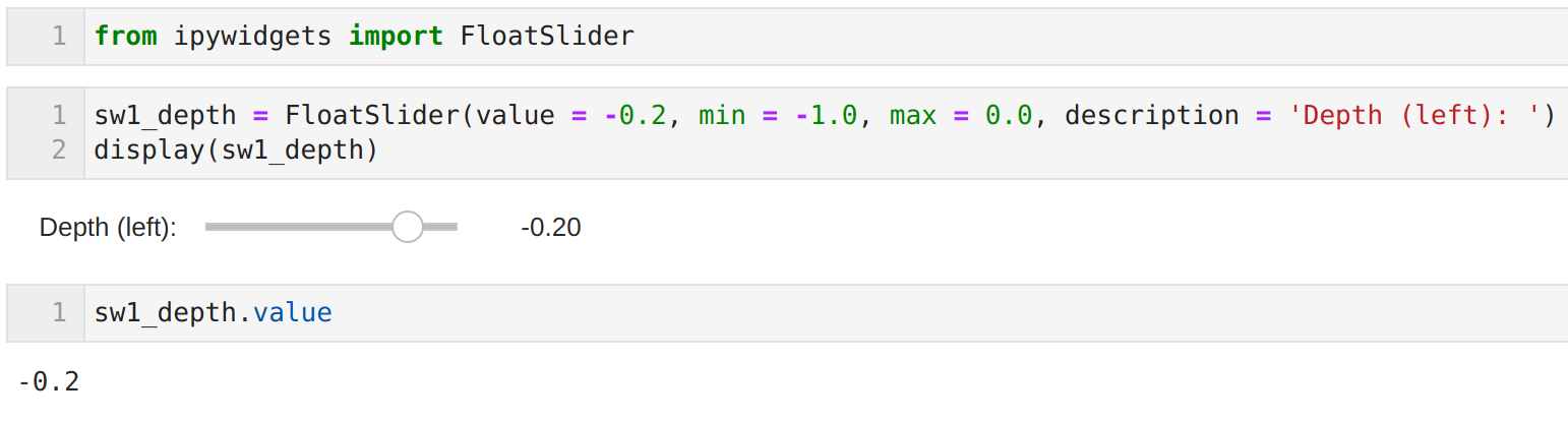
Figure 7: Creation of a slider widget (from the ipywidgets package) to enable the user to control a (floating point) numerical value. The parameters passed to the initializer allow to decide the default initial value and the range (min, max) of allowed inputs, together with a textual description of the widget. In subsequent cells, it is possible (from Python) to retrieve the current value of the widget, or set its value programmatically, using the .value property.

Beside being able to check the value of the slider in specific points of the code, an essential part of the interactivity comes from a very small time delay between user actions (button clicks, change of the value of a slider, …) and the adaptive reaction of the notebook. In OSSCAR, this is achieved using the traitlets library [61]. In particular, every time the attributes of a widget are modified, the widget emits an event of type “change”. We can then define callback functions that are triggered every time there is a change, and bind them to the event using the observe method of the widget. For instance, in Fig. 8 we show a code snippet defining a callback function slider_value_change to replot the function in the figure generated using axes[0].plot discussed in B after changes triggered by the sw1_depth slider.

⬇

1# define the callback function to replot

2def slider_value_change(c):

3 ...

4 axes[0].plot(x, V)

5 ...

6

7# bind the callback, so that it is triggered every time

8# that the value of sw1_depth changes

9sw1_depth.observe(slider_value_change, names="value")

Figure 8: A minimal example of how to define a callback and bind it to any change of value of the slider of Fig. 7.

Finally, we mention that events can be associated to any widget, including plots, thus allowing to tune the value of certain parameters not only from the controllers section, but also by clicking directly on the visualizations (and, in this case, adapting the value of the controllers accordingly). This approach allows for the implementation of reciprocative dynamic linking between components, that has been shown to improve representational competence in students [62].

References

- [1] T. de Jong, M. C. Linn, Z. C. Zacharia, Physical and virtual laboratories in science and engineering education, Science 340 (6130) (2013) 305–308.
- [2] M. Joffre, Quantum physics online, https://www.quantum-physics.polytechnique.fr (2019).
- [3] F. Smallenburg, L. Filion, R. M. Alkemade, A. Ulugöl, Soft matter demos, https://www.softmatterdemos.org (2022).
- [4] Network for Computational Nanotechnology, Nanohub, https://nanohub.org (2022).
- [5] The LabXchange team, Labxchange, https://www.labxchange.org (2022).
- [6] W. Vallejo, C. Díaz-Uribe, C. Fajardo, Google colab and virtual simulations: Practical e-learning tools to support the teaching of thermodynamics and to introduce coding to students, ACS Omega (Feb. 2022).
- [7] H. Kawasaki, S. Yamasaki, Y. Masuoka, M. Iwasa, S. Fukita, R. Matsuyama, Remote teaching due to covid-19: An exploration of its effectiveness and issues, International Journal of Environmental Research and Public Health 18 (5) (2021).
- [8] M. Youmans, Going remote: How teaching during a crisis is unique to other distance learning experiences, J. Chem. Educ. 97 (9) (2020) 3374––3380.
- [9] M. M. Zalat, M. S. Hamed, S. A. Bolbol, The experiences, challenges, and acceptance of e-learning as a tool for teaching during the covid-19 pandemic among university medical staff, PLOS ONE 16 (3) (03 2021).
- [10] Z. Almahasees, K. Mohsen, M. O. Amin, Faculty’s and students’ perceptions of online learning during covid-19, Frontiers in Education 6 (2021).
- [11] J. R. Hoehn, M. F. J. Fox, A. Werth, V. Borish, H. J. Lewandowski, Remote advanced lab course: A case study analysis of open-ended projects, Phys. Rev. Phys. Educ. Res. 17 (2021) 020111.
- [12] R. Kobayashi, T. P. M. Goumans, N. O. Carstensen, T. M. Soini, N. Marzari, I. Timrov, S. Poncé, E. B. Linscott, C. J. Sewell, G. Pizzi, F. Ramirez, M. Bercx, S. P. Huber, C. S. Adorf, L. Talirz, Virtual computational chemistry teaching laboratories—hands-on at a distance, Journal of Chemical Education 98 (10) (2021) 3163–3171.
- [13] A. V. Yakutovich, K. Eimre, O. Schütt, L. Talirz, C. S. Adorf, C. W. Andersen, E. Ditler, D. Du, D. Passerone, B. Smit, N. Marzari, G. Pizzi, C. A. Pignedoli, Aiidalab – an ecosystem for developing, executing, and sharing scientific workflows, Computational Materials Science 188 (2021) 110165.
- [14] T. Kluyver, B. Ragan-Kelley, F. Pérez, B. Granger, M. Bussonnier, J. Frederic, K. Kelley, J. Hamrick, J. Grout, S. Corlay, P. Ivanov, D. Avila, S. Abdalla, C. Willing, J. development team, Jupyter notebooks - a publishing format for reproducible computational workflows, in: F. Loizides, B. Scmidt (Eds.), Positioning and Power in Academic Publishing: Players, Agents and Agendas, IOS Press, Netherlands, 2016, pp. 87–90.
- [15] Project Jupyter, Jupyter, https://docs.jupyter.org (2022).
- [16] B. E. Granger, F. Pérez, Jupyter: Thinking and storytelling with code and data, Computing in Science Engineering 23 (2) (2021) 7–14.
- [17] Project Jupyter, Jupyterlab, https://github.com/jupyterlab/jupyterlab (2022).
- [18] Voila Development Team, Voila, https://github.com/voila-dashboards/voila (2022).
- [19] G. Grosso, G. Pastori Parravicini, Solid State Physics, Academic Press, Oxford, UK, 2013.
- [20] R. R. Hake, Interactive-engagement versus traditional methods: A six-thousand-student survey of mechanics test data for introductory physics courses, American Journal of Physics 66 (1) (1998) 64–74.
- [21] C. Crouch, A. P. Fagen, J. P. Callan, E. Mazur, Classroom demonstrations: Learning tools or entertainment?, American Journal of Physics 72 (6) (2004) 835–838.
- [22] S. Freeman, S. L. Eddy, M. McDonough, M. K. Smith, N. Okoroafor, H. Jordt, M. P. Wenderoth, Active learning increases student performance in science, engineering, and mathematics, Proceedings of the National Academy of Sciences 111 (23) (2014) 8410–8415.
- [23] J. M. Perkel, Programming: Pick up python, Nature 518 (7537) (2015) 125–126.
- [24] PyPi Development Team, Pip, https://pypi.org/project/pip (2021).
- [25] Conda Development Team, Conda, https://docs.conda.io (2021).
- [26] J. M. Perkel, By jupyter, it all makes sense, Nature 563 (7729) (2018) 145–146.
- [27] L. A. Barba, L. J. Barker, D. S. Blank, J. Brown, A. B. Downey, T. George, L. J. Heagy, K. T. Mandli, J. K. Moore, D. Lippert, K. E. Niemeyer, R. R. Watkins, R. H. West, E. Wickes, C. Willing, , M. Zingale, Teaching and learning with jupyter, https://jupyter4edu.github.io/jupyter-edu-book (2019).
- [28] C. J. Weiss, Scientific computing for chemists: An undergraduate course in simulations, data processing, and visualization, Journal of Chemical Education 94 (5) (2017) 592–597. doi:10.1021/acs.jchemed.7b00078.
- [29] J. K. Gilbert, M. Reiner, M. Nakhleh, Visualization: Theory and practice in science education, Springer Netherlands, 2008.
- [30] H. Nguyen, D. A. Case, A. S. Rose, NGLview–interactive molecular graphics for jupyter notebooks, Bioinformatics 34 (7) (2017) 1241–1242.
- [31] Y. Hinuma, G. Pizzi, Y. Kumagai, F. Oba, I. Tanaka, Band structure diagram paths based on crystallography, Computational Materials Science 128 (2017) 140–184.
- [32] D. J. Clarke, M. Jeon, D. J. Stein, N. Moiseyev, E. Kropiwnicki, C. Dai, Z. Xie, M. L. Wojciechowicz, S. Litz, J. Hom, J. E. Evangelista, L. Goldman, S. Zhang, C. Yoon, T. Ahamed, S. Bhuiyan, M. Cheng, J. Karam, K. M. Jagodnik, I. Shu, A. Lachmann, S. Ayling, S. L. Jenkins, A. Ma’ayan, Appyters: Turning jupyter notebooks into data-driven web apps, Patterns 2 (3) (2021) 100213.
- [33] S. Lau, J. Hug, nbinteract: generate interactive web pages from jupyter notebooks, Master’s thesis, EECS Department, University of California, Berkeley (2018).
- [34] Bokeh Development Team, Bokeh: Python library for interactive visualization, https://bokeh.pydata.org/en/latest (2018).
- [35] Ole Schütt, appmode, https://github.com/oschuett/appmode (2022).
- [36] Jupyter Development Team, nbconvert, https://nbconvert.readthedocs.io (2022).
- [37] Jupyter Book Community, Jupyter book, https://jupyterbook.org (2022).
- [38] B. Kim, G. Henke, Easy-to-use cloud computing for teaching data science, Journal of Statistics and Data Science Education 29 (sup1) (2021) S103–S111.
- [39] Docker, Inc., Docker, https://www.docker.com (2021).
- [40] Dokku Development Team, Dokku: The smallest paas implementation you’ve ever seen, https://dokku.com (2021).
- [41] L. Talirz, S. Kumbhar, E. Passaro, A. V. Yakutovich, V. Granata, F. Gargiulo, M. Borelli, M. Uhrin, S. P. Huber, S. Zoupanos, C. S. Adorf, C. W. Andersen, O. Schütt, C. A. Pignedoli, D. Passerone, J. VandeVondele, T. C. Schulthess, B. Smit, G. Pizzi, N. Marzari, Materials cloud, a platform for open computational science, Scientific Data 7 (1) (2020) 299.
- [42] Google LLC, Google Colab, https://colab.research.google.com (2022).
- [43] D. Frenkel, B. Smit, Understanding molecular simulation: from algorithms to applications, Vol. 1, Elsevier, San Diego, 2001.
- [44] W. H. Press, B. P. Flannery, S. A. Teukolsky, W. T. Vetterling, Numerical recipes in C, The Art of Scientific Computing, Second Edition, Cambridge University Press, Cambridge, 1992.
- [45] S. Ainsworth, The multiple representation principle in multimedia learning, in: R. Mayer (Ed.), The Cambridge Handbook of Multimedia Learning, Cambridge University Press, 2014, pp. 464–486.
- [46] J. Izaac, J. Wang, Computational quantum mechanics, Springer, 2018.
- [47] R. Shankar, Principles of quantum mechanics, Springer Science & Business Media, 2012.
- [48] D. J. Tannor, Introduction to quantum mechanics: a time-dependent perspective, University Science Books, Sausalito, California, 2007.
- [49] J. Thijssen, Computational Physics, Cambridge University Press, Delft, 2007.
- [50] J. A. Fleck, J. Morris, M. Feit, Time-dependent propagation of high energy laser beams through the atmosphere, Applied physics 10 (2) (1976) 129–160.
- [51] C. H. Crouch, E. Mazur, Peer instruction: Ten years of experience and results, American Journal of Physics 69 (9) (2001) 970–977.
- [52] C. R. Harris, K. J. Millman, S. J. van der Walt, R. Gommers, P. Virtanen, D. Cournapeau, E. Wieser, J. Taylor, S. Berg, N. J. Smith, R. Kern, M. Picus, S. Hoyer, M. H. van Kerkwijk, M. Brett, A. Haldane, J. F. del Río, M. Wiebe, P. Peterson, P. Gérard-Marchant, K. Sheppard, T. Reddy, W. Weckesser, H. Abbasi, C. Gohlke, T. E. Oliphant, Array programming with numpy, Nature 585 (7825) (2020) 357–362.
- [53] P. Virtanen, R. Gommers, T. E. Oliphant, M. Haberland, T. Reddy, D. Cournapeau, E. Burovski, P. Peterson, W. Weckesser, J. Bright, S. J. van der Walt, M. Brett, J. Wilson, K. J. Millman, N. Mayorov, A. R. J. Nelson, E. Jones, R. Kern, E. Larson, C. J. Carey, İ. Polat, Y. Feng, E. W. Moore, J. VanderPlas, D. Laxalde, J. Perktold, R. Cimrman, I. Henriksen, E. A. Quintero, C. R. Harris, A. M. Archibald, A. H. Ribeiro, F. Pedregosa, P. van Mulbregt, A. Vijaykumar, A. P. Bardelli, A. Rothberg, A. Hilboll, A. Kloeckner, A. Scopatz, A. Lee, A. Rokem, C. N. Woods, C. Fulton, C. Masson, C. Häggström, C. Fitzgerald, D. A. Nicholson, D. R. Hagen, D. V. Pasechnik, E. Olivetti, E. Martin, E. Wieser, F. Silva, F. Lenders, F. Wilhelm, G. Young, G. A. Price, G.-L. Ingold, G. E. Allen, G. R. Lee, H. Audren, I. Probst, J. P. Dietrich, J. Silterra, J. T. Webber, J. Slavič, J. Nothman, J. Buchner, J. Kulick, J. L. Schönberger, J. V. de Miranda Cardoso, J. Reimer, J. Harrington, J. L. C. Rodríguez, J. Nunez-Iglesias, J. Kuczynski, K. Tritz, M. Thoma, M. Newville, M. Kümmerer, M. Bolingbroke, M. Tartre, M. Pak, N. J. Smith, N. Nowaczyk, N. Shebanov, O. Pavlyk, P. A. Brodtkorb, P. Lee, R. T. McGibbon, R. Feldbauer, S. Lewis, S. Tygier, S. Sievert, S. Vigna, S. Peterson, S. More, T. Pudlik, T. Oshima, T. J. Pingel, T. P. Robitaille, T. Spura, T. R. Jones, T. Cera, T. Leslie, T. Zito, T. Krauss, U. Upadhyay, Y. O. Halchenko, Y. Vázquez-Baeza, S. 1.0 Contributors, Scipy 1.0: fundamental algorithms for scientific computing in python, Nature Methods 17 (3) (2020) 261–272.
- [54] S. K. Lam, A. Pitrou, S. Seibert, Numba: a llvm-based python jit compiler, Proceedings of the Second Workshop on the LLVM Compiler Infrastructure in HPC (2015).
- [55] S. Behnel, R. Bradshaw, C. Citro, L. Dalcin, D. S. Seljebotn, K. Smith, Cython: The best of both worlds, Computing in Science Engineering 13 (2) (2011) 31–39.
- [56] NumPy Developers, F2py user guide and reference manual, https://numpy.org/doc/stable/f2py (2021).
- [57] J. D. Hunter, Matplotlib: A 2d graphics environment, Computing in Science & Engineering 9 (3) (2007) 90–95.
- [58] Jon Mease, Bringing ipywidgets Support to plotly.py, in: Fatih Akici, David Lippa, Dillon Niederhut, M. Pacer (Eds.), Proceedings of the 17th Python in Science Conference, 2018, pp. 69 – 76.
- [59] bqplot Development Team, bqplot, https://github.com/bqplot/bqplot (2022).
- [60] J. AHRENS, B. GEVECI, C. LAW, 36 - paraview: An end-user tool for large-data visualization, in: C. D. Hansen, C. R. Johnson (Eds.), Visualization Handbook, Butterworth-Heinemann, Burlington, 2005, pp. 717–731.
- [61] IPython Development Team, Traitlets, https://traitlets.readthedocs.io (2015).
- [62] M. Patwardhan, S. Murthy, Designing reciprocative dynamic linking to improve learners’ representational competence in interactive learning environments, Research and Practice in Technology Enhanced Learning 12 (2017) 10.