Shifting physics of vortex particles to higher energies
via quantum entanglement

Abstract

Physics of structured waves is currently limited to relatively small particle energies as the available generation techniques are only applicable to the soft $X$-ray twisted photons, to the beams of electron microscopes, to cold neutrons, or non-relativistic atoms. The highly energetic vortex particles with an orbital angular momentum would come in handy for a number of experiments in atomic physics, nuclear, hadronic, and accelerator physics, and to generate them one needs to develop alternative methods, applicable for ultrarelativistic energies and for composite particles. Here, we show that the vortex states of in principle arbitrary particles can be generated during photon emission in helical undulators, via Cherenkov radiation, in collisions of charged particles with intense laser beams, in such scattering or annihilation processes as $e\mu\to e\mu,ep\to ep,e^{-}e^{+}\to p\bar{p}$, and so forth. The key element in obtaining them is the postselection protocol due to entanglement between a pair of final particles and it is largely not the process itself. The state of a final particle – be it a $\gamma$-ray, a hadron, a nucleus, or an ion – becomes twisted if the azimuthal angle of the other particle momentum is measured with a large error or is not measured at all. As a result, requirements to the beam transverse coherence can be greatly relaxed, which enables the generation of highly energetic vortex beams at accelerators and synchrotron radiation facilities, thus making them a new tool for hadronic and spin studies.

1 Introduction

Photons with an orbital angular momentum (OAM) [1] have found applications in quantum optics and information, optomechanics, biology, astrophysics, and in other fields [2, 3, 4, 5, 6, 7, 8, 9]. They can be entangled in the polarization and orbital degrees of freedom [10, 11] and their OAM quanta can reach the values of 10010$\hbar$[12]. Along with the diffraction techniques, such twisted light can be generated by charged particles in helical undulators [13, 14, 15, 16, 17, 18, 19], via non-linear Thomson or Compton scattering [19, 20, 21, 22, 23] or – more generally – when the electron trajectory is helical [24, 25, 26], during Cherenkov or transition radiation [27, 28], via channeling in crystals [29, 30], and so forth. However, despite the proposals to use twisted photons in particle and nuclear studies [6], their highest energy achieved so far does not exceed but a few keV [7]. One recent idea to upconvert their frequency is to employ resonant scattering of the optical twisted photons on relativistic ions within the Gamma Factory project at the Large Hadron Collider [6, 31].

The massive counterparts of twisted photons – the vortex electrons [32, 33] – have been generated with the moderately relativistic beams of transmission electron microscopes [34, 35, 36, 33] and with a non-relativistic beam of a scanning microscope [37]. Their OAM can be as high as $1000\hbar$ [38, 39] resulting in a larger magnetic moment compared to that of a plane-wave electron and they can be useful for probing magnetic properties of materials, chirality in crystals, etc. [40, 33]. These electron packets have also attracted attention outside the microscopy community because of the potential applications in atomic and high-energy physics [32, 33, 41, 42, 43, 44, 45, 46, 47, 48, 49, 50, 51, 52, 53, 54, 55, 56, 57, 58, 59, 60, 61, 62, 63] and, in particular, in hadronic and spin studies – see the recent review [64]. They can even come in handy in accelerator physics [65, 66] where their classical counterparts – the angular-momentum-dominated beams – have been utilized since the beginning of 2000s with the beam vorticity being analogous to the intrinsic OAM of a particle (see [67, 68, 69, 70] and references therein).

There are ongoing discussions of the possible experiments with vortex muons, hadrons, ions and atoms, cold neutrons, nuclei, spin waves (magnons), etc. [45, 46, 52, 55, 56, 57, 58, 72, 59, 60, 65, 66, 8, 71, 62]. Very recently, in 2021, the non-relativistic twisted atoms and molecules have been generated [73]. Although a large class of quantum and classical waves can carry phase vortices, the available diffraction techniques to generate them [34, 35, 36, 74, 75] require beams with the large transverse coherence and they are hardly applicable for relativistic beams of accelerators. This circumstance severely limits the development of physics of structured waves to higher energies.

Indeed, even if the electron beam current is low and there is no space-charge, the Rayleigh length of a relativistic electron packet is usually much larger than the length of the collision region inside a linac, whereas in a storage ring the rms-width $\sqrt{\langle\rho^{2}\rangle}$ of a charged-particle packet does not grow but oscillates [66, 76, 77, 78], revealing quantum betatron oscillations or broadening of the classical trajectories [79]. Therefore, the transverse coherence length of a packet naturally remains small, and the corresponding quantum effects do not play any role in collider experiments. To bring physics of the non-Gaussian matter waves to the high-energy domain, alternative methods for generating the vortex states of a large class of quantum systems are needed. Several such techniques have been discussed by one of us in [65, 66] and it was shown that it is possible to accelerate vortex electrons up to ultrarelativistic energies by modifying the particle sources.

In this paper, we further elaborate our ideas from Ref.[80] and describe a method to generate vortex states of particles of in principle arbitrary mass, spin, and energy, including hard X-ray and $\gamma$-range photons, muons, protons, ions and nuclei. They can be obtained during emission of photons in accelerators and free-electron lasers, via scattering or annihilation processes with leptons and hadrons, such as

$$e\mu\to e\mu,\,ep\to ep,\,e^{-}e^{+}\to h\bar{h},\,e^{-}e^{+}\to 2\gamma,$$ (1)

scattering of light on relativistic ions, discussed within the Gamma Factory project [6, 81], etc. Our key observation is that it is largely not the process itself that defines vorticity of a final particle, but rather it is a post-selection protocol due to entanglement between the final particles. Whereas in the classical realm the radiation is twisted if the emitting electron path is helical [24], the more general quantum theory developed here predicts that photons cannot be twisted at all if the emitting particle 3-momentum ${\bf p}^{\prime}$ is precisely measured, and that their OAM depends on the way we post-select the electron. Our results complement and specify those of the classical theory, but also make them somewhat less optimistic because the conventional post-selection protocol [82, 83] results in no vorticity of the emitted photons whatsoever.

We point out a deep analogy between a generalized measurement [84, 85] of a particle momentum ${\bm{p}}^{\prime}=\{p^{\prime}_{x},p^{\prime}_{y},p^{\prime}_{z}\}=\{p^{\prime}_{\perp}\cos\phi^{\prime},p^{\prime}_{\perp}\sin\phi^{\prime},p^{\prime}_{z}\}$, in which not all the components are measured with a vanishing error, and a standard von Neumann measurement in cylindrical basis [45], in which the azimuthal angle $\phi^{\prime}=\arctan(p^{\prime}_{y}/p^{\prime}_{x})$ does not belong to the measurable set of quantum numbers. If this angle is measured with a very large error, this lack of information is enough for the state of the other final particle to become twisted, thanks to entanglement and to the angle-OAM uncertainty relation [86, 87].

The crucial advantage of this technique is that neither modifications of the incoming beams are required nor there are limitations due to their small transverse coherence. To generate the vortex state of any particle – be it a $\gamma$-ray, a proton, or a nucleus in a reaction with two final particles – it is enough to measure the azimuthal angle of the other particle with a large error or not to measure it at all. This method can be employed for the generation of highly energetic vortex beams at the electron and hadron accelerators, X-ray free-electron lasers and synchrotron radiation facilities with helical undulators such as, for instance, the European XFEL and ESRF, powerful laser facilities such as the Extreme Light Infrastructure, and at the future linear colliders. A system of units with $\hbar=c=1$ is used.

2 Evolved state of the final particles

Let us start with emission of a photon by a charged particle,

$$e\to e^{\prime}+\gamma,$$ (2)

in the lowest order of the perturbation theory in QED. Generalizations to the scattering and annihilation processes are straightforward. For definiteness, we will take an electron in what follows. It can generate either Cherenkov radiation or transition radiation, synchrotron radiation, undulator radiation in a given electromagnetic field, and so on. A quantum state of the final system as it evolves from the reaction irrespectively of the measurement protocol can be called pre-selected or evolved because no measurements have been done yet. An initial state $|\text{in}\rangle$ of the electron and an evolved state of the final system $|\text{ev}\rangle$ are connected via an evolution operator $\hat{S}$ [82, 83]

$$|\text{ev}\rangle=\hat{S}\,|\text{in}\rangle,\ \hat{S}=\text{T}\exp\left\{-ie\int d^{4}x\,\hat{j}_{\mu}\hat{A}^{\mu}\right\}.$$ (3)

In what follows, we restrict ourselves only to the first-order QED processes with $\hat{S}=\hat{S}^{(1)}$ for which the evolved state consists of the electron and the photon, $|\text{ev}\rangle=|e^{\prime},\gamma\rangle^{(\text{ev})}$. In this case,

$$|e^{\prime},\gamma\rangle^{(\text{ev})}=\hat{S}^{(1)}\,|\text{in}\rangle=\sum\limits_{f}|f\rangle\langle f|\hat{S}^{(1)}|\text{in}\rangle,$$ (4)

where we have expanded the unitary operator over a complete set of two-particle states (with no virtual particles)

$$\hat{1}=\sum\limits_{f}|f\rangle\langle f|=\sum\limits_{f_{e}}\sum\limits_{f_{\gamma}}|f_{e},f_{\gamma}\rangle\langle f_{e},f_{\gamma}|.$$ (5)

In particular, this can be the plane-wave states of free particles with the definite momenta ${\bm{p}},{\bm{k}}$, the energies $\varepsilon=\sqrt{m_{e}^{2}+{\bm{p}}^{2}},\omega=|{\bm{k}}|$, and the helicities $\lambda=\pm 1/2,\lambda_{\gamma}=\pm 1$, so that

$$\hat{1}=\sum\limits_{\lambda_{\gamma}\lambda}\int\frac{d^{3}p}{(2\pi)^{3}}\frac{d^{3}k}{(2\pi)^{3}}|{\bf k},\lambda_{\gamma};{\bf p},\lambda\rangle\langle{\bf p},\lambda;{\bf k},\lambda_{\gamma}|.$$ (6)

In this case, the average

$$S_{fi}^{(1)}=\langle f_{e},f_{\gamma}|\hat{S}^{(1)}|\text{in}\rangle=\langle{\bf p},\lambda;{\bf k},\lambda_{\gamma}|\hat{S}^{(1)}|\text{in}\rangle$$ (7)

is a customary firs-order matrix element with two final plane-wave states.

Let us first assume that no final particle is detected and discuss how one can describe the entangled evolved state. The field operators in the Heisenberg representation of the photon and of the electron are expanded into series of the creation and annihilation operators of the freely propagating plane-wave states

$$\displaystyle\hat{\bm{A}}({\bm{r}},t)=\sum\limits_{\lambda_{\gamma}=\pm 1}\int\frac{d^{3}k}{(2\pi)^{3}}\left({\bm{A}}_{{\bm{k}}\lambda_{\gamma}}({\bm{r}},t)\,\hat{c}_{{\bm{k}}\lambda_{\gamma}}+\text{h.c.}\right),\,{\bm{A}}_{{\bm{k}}\lambda_{\gamma}}({\bm{r}},t)=\frac{\sqrt{4\pi}}{\sqrt{2\omega}}\,{\bm{e}}_{{\bm{k}}\lambda_{\gamma}}\,e^{-i\omega t+i{\bm{k}}\cdot{\bm{r}}},$$ (8)

$$\displaystyle\hat{\psi}({\bm{r}},t)=\sum\limits_{\lambda=\pm 1/2}\int\frac{d^{3}p}{(2\pi)^{3}}\psi_{{\bm{p}}\lambda}({\bm{r}},t)\hat{a}_{{\bm{p}}\lambda},\,\psi_{{\bm{p}}\lambda}({\bm{r}},t)=\frac{1}{\sqrt{2\varepsilon}}\,u_{{\bm{p}}\lambda}\,e^{-i\varepsilon t+i{\bm{p}}\cdot{\bm{r}}},$$ (9)

where we have omitted the positron part. Note that for Cherenkov radiation in a transparent medium with a refraction index $\tilde{n}(\omega)$, we have $\omega=|\bm{k}|/\tilde{n}$ and the normalization factor must be $1/\sqrt{2\omega}\to 1/\tilde{n}\sqrt{2\omega}$, see Ref.[50] and Sec. 4 below. Now, following the standard interpretation [82, 83, 88], one can define the two-particle evolved state in 4-dimensional space-time as follows:

$$\displaystyle\langle 0|\hat{\psi}({\bm{r}}_{e},t_{e})\hat{{\bm{A}}}({\bm{r}}_{\gamma},t_{\gamma})|e^{\prime},\gamma\rangle^{(\text{ev})}=$$ (10)

$$\displaystyle=\int\frac{d^{3}p}{(2\pi)^{3}}\frac{d^{3}k}{(2\pi)^{3}}\,\sum\limits_{\lambda_{\gamma}=\pm 1}\sum\limits_{\lambda=\pm 1/2}\frac{\sqrt{4\pi}}{\sqrt{2\omega}}\frac{1}{\sqrt{2\varepsilon}}\,u_{{\bm{p}}\lambda}\,{\bm{e}}_{{\bm{k}}\lambda_{\gamma}}\,S_{fi}^{(1)}\,e^{-i\varepsilon t_{e}+i{\bm{p}}\cdot{\bm{r}}_{e}-i\omega t_{\gamma}+i{\bm{k}}\cdot{\bm{r}}_{\gamma}},$$ (11)

with $S_{fi}^{(1)}$ from (7). This average yields the probability amplitude to detect the photon at the time instant $t_{\gamma}$ in a region of space centered at the point ${\bm{r}}_{\gamma}$, whereas the electron is detected in the region centered at the point $(t_{e},{\bm{r}}_{e})$. So the combination

$$\sum\limits_{\lambda_{\gamma}=\pm 1}\sum\limits_{\lambda=\pm 1/2}u_{{\bm{p}}\lambda}\,{\bm{e}}_{{\bm{k}}\lambda_{\gamma}}\,S_{fi}^{(1)}$$ (12)

plays a role of the wave function of the 2-particle evolved state in the momentum representation, up to the factor $\sqrt{4\pi}/\sqrt{2\omega}\sqrt{2\varepsilon}$.

Now let us assume that only one of the final particles is detected. Say, if the electron is post-selected to the state $|e^{\prime}\rangle$, the evolved state of the photon alone looks as

$$|\gamma\rangle^{(\text{ev})}=\sum\limits_{f_{\gamma}}|f_{\gamma}\rangle\langle e^{\prime};f_{\gamma}|\hat{S}^{(1)}|\text{in}\rangle\equiv\sum\limits_{f_{\gamma}}|f_{\gamma}\rangle S_{fi}^{(1)},$$ (13)

or when the plane-wave basis is used

$$|\gamma\rangle^{(\text{ev})}=\sum\limits_{\lambda_{\gamma}}\int\frac{d^{3}k}{(2\pi)^{3}}|{\bm{k}},\lambda_{\gamma}\rangle\langle e^{\prime};{\bm{k}},\lambda_{\gamma}|\hat{S}^{(1)}|\text{in}\rangle\equiv\sum\limits_{\lambda_{\gamma}}\int\frac{d^{3}k}{(2\pi)^{3}}|{\bm{k}},\lambda_{\gamma}\rangle S_{fi}^{(1)}.$$ (14)

Analogously, if the photon is detected in a state $|\gamma\rangle$, the electron evolved state becomes

$$|e^{\prime}\rangle^{(\text{ev})}=\sum\limits_{f_{e}}|f_{e}\rangle\langle\gamma;f_{e}|\hat{S}^{(1)}|\text{in}\rangle\equiv\sum\limits_{f_{e}}|f_{e}\rangle S_{fi}^{(1)},$$ (15)

or

$$|e^{\prime}\rangle^{(\text{ev})}=\sum\limits_{\lambda}\int\frac{d^{3}p}{(2\pi)^{3}}|{\bm{p}},\lambda\rangle S_{fi}^{(1)}.$$ (16)

One can treat the averages

$$\displaystyle{\bm{A}}^{(\text{ev})}({\bm{r}},t)\equiv\langle 0|\hat{\bm{A}}({\bm{r}},t)|\gamma\rangle^{(\text{ev})}=\sum\limits_{\lambda_{\gamma}}\int\frac{d^{3}k}{(2\pi)^{3}}\,\frac{\sqrt{4\pi}}{\sqrt{2\omega}}\,{\bm{e}}_{{\bm{k}}\lambda_{\gamma}}\,\langle{\bm{k}},\lambda_{\gamma}|\gamma\rangle^{(\text{ev})}\,e^{-i\omega t+i{\bm{k}}\cdot{\bm{r}}},$$ (17)

$$\displaystyle\psi^{(\text{ev})}({\bm{r}},t)\equiv\langle 0|\hat{\psi}({\bm{r}},t)|e^{\prime}\rangle^{(\text{ev})}=\sum\limits_{\lambda}\int\frac{d^{3}p}{(2\pi)^{3}}\,\frac{1}{\sqrt{2\varepsilon}}\,u_{{\bm{p}}\lambda}\langle{\bm{p}},\lambda|e^{\prime}\rangle^{(\text{ev})}e^{-i\varepsilon t+i{\bm{p}}\cdot{\bm{r}}}$$ (18)

as the probability amplitudes to detect the corresponding particle in the region of space-time centered at the point $(t,{\bm{r}})$. In particular, if the photon evolved state is the plane wave, $|\gamma\rangle^{(\text{ev})}=|{\bm{k}}^{\prime},\lambda^{\prime}\rangle$, then

$$\langle 0|\hat{\bm{A}}({\bm{r}},t)|{\bm{k}}^{\prime},\lambda^{\prime}\rangle={\bm{A}}_{{\bm{k}}^{\prime}\lambda^{\prime}_{\gamma}}({\bm{r}},t)$$ (19)

from Eq.(9) due to the orthogonality condition,

$$\langle{\bm{k}},\lambda_{\gamma}|{\bm{k}}^{\prime},\lambda_{\gamma}^{\prime}\rangle=\langle 0|\hat{c}_{{\bm{k}}\lambda_{\gamma}}\hat{c}^{\dagger}_{{\bm{k}}^{\prime}\lambda^{\prime}_{\gamma}}|0\rangle=(2\pi)^{3}\delta({\bm{k}}-{\bm{k}}^{\prime})\delta_{\lambda_{\gamma}\lambda^{\prime}_{\gamma}}.$$ (20)

As the plane wave is completely delocalized in time and space, it is generally the function

$$\displaystyle\sum\limits_{\lambda_{\gamma}}{\bm{e}}_{{\bm{k}}\lambda_{\gamma}}\,\langle{\bm{k}},\lambda_{\gamma}|\gamma\rangle^{(\text{ev})}=\sum\limits_{\lambda_{\gamma}}{\bm{e}}_{{\bm{k}}\lambda_{\gamma}}\,S_{fi}^{(1)},\ S_{fi}^{(1)}=\langle e^{\prime};{\bm{k}},\lambda_{\gamma}|\hat{S}^{(1)}|\text{in}\rangle,$$ (21)

that has a sense of the photon wave function in the momentum representation [82]. Analogously, the electron wave function is

$$\displaystyle\sum\limits_{\lambda=\pm 1/2}u_{{\bm{p}}\lambda}S_{fi}^{(1)},\ S_{fi}^{(1)}=\langle\gamma;{\bf p},\lambda|\hat{S}^{(1)}|\text{in}\rangle,$$ (22)

when the photon detected state $|\gamma\rangle$ is given.

Importantly, the 1-particle functions (18) can be treated as the probability amplitudes only when the other particle is also detected at a finite point of space-time, and its state represents a spatially localized wave packet. Indeed, let us assume the opposite: the incoming electron is a plane wave $|{\bf p},\lambda\rangle$ and the final electron is also detected in the delocalized plane-wave state $|e^{\prime}\rangle=|{\bf p}^{\prime},\lambda^{\prime}\rangle$ (say, during Cherenkov radiation). Then the photon evolved state becomes

$$\displaystyle{\bm{A}}^{(\text{ev})}({\bm{r}},t)=\sum\limits_{\lambda_{\gamma}}\int\frac{d^{3}k}{(2\pi)^{3}}\,\frac{\sqrt{4\pi}}{\sqrt{2\omega}}\,{\bm{e}}_{{\bm{k}}\lambda_{\gamma}}\,S_{fi}^{(1)}\,e^{-i\omega t+i{\bm{k}}\cdot{\bm{r}}},$$ (23)

$$\displaystyle S_{fi}^{(1)}=\langle{\bf p}^{\prime},\lambda^{\prime};{\bf k},\lambda_{\gamma}|\hat{S}^{(1)}|{\bf p},\lambda\rangle\propto\delta^{(4)}(p-p^{\prime}-k).$$ (24)

The integral over $d^{3}k$ is done with the momenta delta-function, and ${\bm{A}}^{(\text{ev})}({\bm{r}},t)$ stays proportional to $\delta(\varepsilon-\varepsilon^{\prime}-\omega)=(2\pi)^{-1}\int_{t_{\text{in}}=-\infty}^{t_{\text{out}}=+\infty}dt\,\exp\left\{it(\varepsilon-\varepsilon^{\prime}-\omega)\right\}$, due to the infinite limits in the time integral. To circumvent this singular behavior, one can take the final particle (electron or photon) as a localized packet with a detector function $f_{p}({\bf p}^{\prime})$,

$$\displaystyle|e^{\prime}\rangle=\int\frac{d^{3}p^{\prime}}{(2\pi)^{3}}f_{p}({\bf p}^{\prime})|{\bf p}^{\prime},\lambda^{\prime}\rangle,$$ (25)

$$\displaystyle\langle e^{\prime}|e^{\prime}\rangle=\int\frac{d^{3}p^{\prime}}{(2\pi)^{3}}|f_{p}({\bf p}^{\prime})|^{2}=1,$$ (26)

where we have used

$$\langle{\bm{p}},\lambda|{\bm{p}}^{\prime},\lambda^{\prime}\rangle=(2\pi)^{3}\delta({\bm{p}}-{\bm{p}}^{\prime})\delta_{\lambda\lambda^{\prime}}.$$ (27)

Then the evolved states become

$$\displaystyle{\bm{A}}^{(\text{ev})}({\bm{r}},t)=\sum\limits_{\lambda_{\gamma}}\int\frac{d^{3}k}{(2\pi)^{3}}\frac{d^{3}p^{\prime}}{(2\pi)^{3}}\,f_{p}^{*}({\bf p}^{\prime})\,\frac{\sqrt{4\pi}}{\sqrt{2\omega}}\,{\bm{e}}_{{\bm{k}}\lambda_{\gamma}}\,S_{fi}^{(1)}\,e^{-i\omega t+i{\bm{k}}\cdot{\bm{r}}},$$ (28)

$$\displaystyle\psi^{(\text{ev})}({\bm{r}},t)=\sum\limits_{\lambda}\int\frac{d^{3}p}{(2\pi)^{3}}\frac{d^{3}k}{(2\pi)^{3}}\,f_{k}^{*}({\bf k})\,\frac{1}{\sqrt{2\varepsilon}}\,u_{{\bm{p}}\lambda}S_{fi}^{(1)}e^{-i\varepsilon t+i{\bm{p}}\cdot{\bm{r}}},$$ (29)

and their momentum counterparts

$$\displaystyle\int\frac{d^{3}p^{\prime}}{(2\pi)^{3}}\,\sum\limits_{\lambda_{\gamma}}f_{p}^{*}({\bf p}^{\prime})\,{\bm{e}}_{{\bm{k}}\lambda_{\gamma}}\,S_{fi}^{(1)}\quad\text{and}\quad\int\frac{d^{3}k}{(2\pi)^{3}}\sum\limits_{\lambda}f_{k}^{*}({\bf k})\,u_{{\bm{p}}\lambda}S_{fi}^{(1)},$$ (30)

depend on the functions $f_{p}({\bf p}^{\prime}),f_{k}({\bf k})$ describing detector properties of the other particle. As the square-integrable functions $f_{p}({\bf p}^{\prime})$ or $f_{k}({\bf k})$ localize the packets spatially and temporarily, the S-matrix element is effectively “regularized”, $S_{fi}^{(1)}\to\int\frac{d^{3}p^{\prime}}{(2\pi)^{3}}\,f_{p}^{*}({\bf p}^{\prime})\,S_{fi}^{(1)}$, so that the evolution now occurs in a finite region of space and during a finite time. The functions (30) keep their sense in the limit $f_{p}({\bf p}^{\prime})\to(2\pi)^{3}\delta({\bf p}^{\prime}-\bar{{\bf p}}^{\prime}),f_{k}({\bf k})\to(2\pi)^{3}\delta({\bf k}-\bar{{\bf k}})$ when they reduce to Eq.(21) and (22), respectively. In this paper, we do not aim at a full description of the detection process in space-time and, therefore, we will mostly study the states in the momentum representation for which $f_{p}({\bf p}^{\prime}),f_{k}({\bf k})$ may not be square-integrable.

Clearly, the above definitions can easily be generalized for scattering and annihilation processes, both elastic and inelastic, including reactions with hadrons, ions, or nuclei in the final state. In the latter case, Eq.(22) can define an evolved wave function of a hadron when all other particles are detected.

We emphasize the difference between the above quantum picture and the classical theory: in the latter the electron path is given, the particle experiences no recoil, the coherent properties and the phase of the radiation field are solely defined by the trajectory. In particular, when the electron path is spiral the radiation field is always twisted [24]. The quantum picture embraces the classical problem as a special case (the correspondence principle), but it is inevitably more complex: the evolved state of the emitted photon always depends on how the emitting particle (electron) is post-selected. As we show below, if the electron 3-momentum is measured via the standard projective measurement approach [83], the final photon turns out to be not twisted at all, even if the electron packet centroid moves along a helix. Thus, the twisted particles may not be that abundant in Nature as it seems to follow from the classical theory.

3 Measurement scenarios

3.1 Projective measurements in plane-wave basis

Let the initial electron be described as a plane-wave state propagating along the $z$ axis with the momentum ${\bf p}=\{0,0,|{\bf p}|\}$ (say, for Cherenkov radiation). Following the conventional textbook approach [82, 83], if it is post-selected to a plane-wave state with the momentum ${\bf p}^{\prime}=\{{\bf p}^{\prime}_{\perp},p^{\prime}_{z}\}$ and the helicity $\lambda^{\prime}$, the matrix element $S_{fi}^{(\text{pw})}$ and the photon’s evolved wave function are both proportional to the momentum conservation delta-function

$$S_{fi}^{(\text{pw})}\propto\delta^{(3)}({\bf p}-{\bf p}^{\prime}-{\bf k})\propto\delta^{(2)}({\bf p}^{\prime}_{\perp}+{\bf k}_{\perp}),$$ (31)

$${\bm{A}}^{(\text{ev})}({\bf k},\omega)\propto\sum\limits_{\lambda_{\gamma}=\pm 1}{\bm{e}}\,\delta({\bf p}^{\prime}_{\perp}+{\bf k}_{\perp}).$$ (32)

As soon as the azimuthal angle $\phi^{\prime}$ of the electron momentum is precisely measured, the photon angle $\phi_{k}$ is also set to a definite value

$$\phi_{k}=\phi^{\prime}\pm\pi.$$ (33)

Thereby, the photon is projected to a plane-wave state without an intrinsic OAM projection on the $z$ axis. One can qualitatively understand this result by recalling the uncertainty relation from Ref.[86, 87], which can be put as follows: a definite azimuthal angle of a plane wave implies a vanishing mean OAM $z$-projection $\langle\hat{L}_{z}\rangle=0$ but an infinitely wide OAM spectrum $\langle\hat{L}^{2}_{z}\rangle=\infty$ (see appendix A for more detail).

Now let us take a general reaction with the plane-wave states, the matrix element of which is proportional to the energy-momentum conservation delta-function [82, 83],

$$S_{fi}^{(\text{pw})}\propto\delta^{(4)}\left(\sum p_{\text{in}}-\sum p_{\text{out}}\right).$$ (34)

If we substitute this to Eq.(21) or (22), we immediately see that the evolved wave function of a photon or of a fermion has a well-defined 4-momentum, which automatically means that $\langle\hat{L}_{z}\rangle=0$.

The projective measurements in the plane-wave basis are most frequently used for describing particle scattering, annihilation, or photon emission. As we have said, in quantum theory it is not the particle trajectory but the post-selection protocol that defines vorticity of the final photon. Therefore, when it comes to the photon phase, direct comparison of the results in the plane-wave basis with the classical theory has a limited sense. Indeed, the classical electron does not experience recoil, so its angle $\phi^{\prime}$ is not defined, which is more similar to the generalized-measurement scheme (iii) below than to the above standard approach.

3.2 Cylindrical basis and generalized measurements

The post-selection to a plane wave represents a projective measurement when all components of the momentum ${\bf p}^{\prime}$ are measured with vanishing errors. During a generalized measurement, on the contrary, at least some of the components are measured with a non-vanishing error (see, e.g., [84, 85]). If the error is maximal, we do not effectively measure this component at all. Put simply, a generalized measurement is the post-selection to a wave packet, a coherent superposition of plane waves,

$$|e^{\prime}_{\text{det}}\rangle^{(\text{g})}=\int\frac{{\displaystyle d^{3}p^{\prime}}}{{\displaystyle(2\pi)^{3}}}\,f_{p}({\bf p}^{\prime})\,|{\bf p}^{\prime},\lambda^{\prime}\rangle,$$ (35)

where the detector function $f_{p}({\bf p}^{\prime})$ is normalized according to Eq.(26). The set of operators

$$|{e^{\prime}_{\text{det}}\rangle}^{(\text{g})}\langle{e^{\prime}_{\text{det}}}|^{(\text{g})}$$ (36)

is complete, although not necessarily orthogonal, and it forms a positive operator-valued measure [84]. There exists a close relative of the generalized measurement, called the weak measurement [89, 90, 91, 92], during which an observable quantity is also measured with a finite error, but the measured weak values do not necessarily belong to the spectrum of the corresponding operator and they can even be complex. The operators (36), needed for our purposes, are hermitian and positively-defined, so the measured values of the azimuthal angle still belong to the interval $[0,2\pi]$, which is why we adhere to the term “generalized measurement” in what follows.

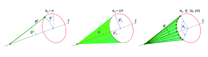
Figure 1: The possible measurement strategies. Left: the conventional plane-wave approach (i) (projective measurement) with the definite 3-momentum ${\bf p}^{\prime}$, middle: the projective measurement in the cylindrical basis (ii) with an undefined azimuthal angle $\phi^{\prime}$ of the momentum, right: the generalized-measurement scheme (iii) with a finite uncertainty $\sigma_{\phi}$ of the azimuthal angle. In all three scenarios, the states are stationary with the definite energy, $\varepsilon^{\prime}=\sqrt{(p^{\prime}_{\perp})^{2}+(p^{\prime}_{z})^{2}+m_{e}^{2}}$.

The detector function can be of the Gaussian form,

$$f_{p}({\bf p}^{\prime})\propto\prod\limits_{i}\exp\left\{-(p^{\prime}_{i}-\langle p_{i}\rangle)^{2}/(2\sigma_{i})^{2}\right\}.$$ (37)

where $i=x,y,z$ or $i=\rho,\phi,z$. A projective measurement implies that $\sigma_{x},\sigma_{y},\sigma_{z}\to 0$. Alternatively, one can use the cylindrical coordinates $p^{\prime}_{\perp},\phi^{\prime}=\arctan(p^{\prime}_{y}/p^{\prime}_{x}),p^{\prime}_{z}$ with the corresponding uncertainties $\sigma_{\perp},\sigma_{\phi},\sigma_{z}$. For a generalized measurement, at least one of these uncertainties is not vanishing.

To provide completeness of the set (36), one generally needs to measure both the non-commutative observables, the simplest example being the coordinates and momenta. The corresponding normalized wave packet can be written as (we omit the helicity sign for now)

$$\displaystyle|e^{\prime}_{\text{det}}\rangle^{(\text{g})}=\left|\langle{\bm{r}}\rangle,\langle{\bm{p}}\rangle\right\rangle=$$ (38)

$$\displaystyle=\int\frac{d^{3}p^{\prime}}{(2\pi)^{3}}\,\prod\limits_{i}\frac{(2\pi)^{3/2}}{(2\pi\sigma_{i}^{2})^{1/4}}\,e^{-\frac{\left(p^{\prime}_{i}-\langle p_{i}\rangle\right)^{2}}{(2\sigma_{i})^{2}}-i\langle{\bm{r}}\rangle\cdot{\bm{p}}^{\prime}}|{\bm{p}^{\prime}}\rangle,$$ (39)

$$\displaystyle\left\langle\langle{\bm{r}}\rangle,\langle{\bm{p}}\rangle|\langle{\bm{r}}\rangle,\langle{\bm{p}}\rangle\right\rangle=1,\ \left\langle\langle{\bm{r}}\rangle,\langle{\bm{p}}\rangle|\hat{{\bm{p}}}|\langle{\bm{r}}\rangle,\langle{\bm{p}}\rangle\right\rangle=\langle{\bm{p}}\rangle,\ \left\langle\langle{\bm{r}}\rangle,\langle{\bm{p}}\rangle|\hat{{\bm{x}}}|\langle{\bm{r}}\rangle,\langle{\bm{p}}\rangle\right\rangle=\langle{\bm{r}}\rangle,$$ (40)

and this set is complete

$$\displaystyle\int d^{3}\langle{\bm{r}}\rangle\frac{d^{3}\langle{\bm{p}}\rangle}{(2\pi)^{3}}\,|\langle{\bm{r}}\rangle,\langle{\bm{p}}\rangle\rangle\langle\langle{\bm{r}}\rangle,\langle{\bm{p}}\rangle|=\int\frac{d^{3}p^{\prime}}{(2\pi)^{3}}\,|{\bm{p}}^{\prime}\rangle\langle{\bm{p}}^{\prime}|=\hat{1}.$$ (41)

These packets represent the so-called coherent states of a freely propagating massive particle [93].

To illustrate these ideas, let us distinguish the following three scenarios (see Fig.1):

(i) We post-select the particles to the plane-wave states and repeat the measurements many times with an ensemble of electrons, each time fixing the detector at a different angle $\phi^{\prime}$. The emission rate or a cross section are proportional to

$$\int\limits_{0}^{2\pi}\frac{{\displaystyle d\phi^{\prime}}}{{\displaystyle 2\pi}}\,|S_{fi}^{\rm(pw)}|^{2},$$ (42)

which represents an incoherent averaging over the azimuthal angle in the projective-measurement scheme. This is the standard textbook approach [82, 83], in which no phases contribute to the observable quantities.

(ii) Another example of a projective measurement is post-selection to a cylindrical wave (a Bessel state) [45] with the definite $p^{\prime}_{\perp},p^{\prime}_{z}$, the $z$-projection of the total angular momentum (TAM) $m^{\prime}$, and the helicity $\lambda^{\prime}$, but undefined angle $\phi^{\prime}$

$$|e^{\prime}_{\text{det}}\rangle=|p^{\prime}_{\perp},p^{\prime}_{z},m^{\prime},\lambda^{\prime}\rangle=$$ (43)

$$=\int\limits_{0}^{2\pi}\frac{{\displaystyle d\phi^{\prime}}}{{\displaystyle 2\pi}}\,i^{-(m^{\prime}-\lambda^{\prime})}e^{i(m^{\prime}-\lambda^{\prime})\phi^{\prime}}\,|{\bf p}^{\prime},\lambda^{\prime}\rangle.$$ (44)

The TAM z-projection operator

$$\hat{j}_{z}=\hat{L}_{z}+\hat{s}_{z},$$ (45)

$$\hat{j}_{z}|p^{\prime}_{\perp},p^{\prime}_{z},m^{\prime},\lambda^{\prime}\rangle=m^{\prime}|p^{\prime}_{\perp},p^{\prime}_{z},m^{\prime},\lambda^{\prime}\rangle,$$ (46)

is a sum of an orbital part $\hat{L}_{z}$ and a spin part $\hat{s}_{z}$. The former is

$$\hat{L}_{z}=[\hat{{\bf r}}\times\hat{{\bf p}}]_{z}=-i\frac{\partial}{\partial\phi},$$ (47)

while the latter depends on the particle spin. Here, $\phi$ refers to the azimuthal angle either of ${\bf r}$ or of ${\bf p}$, depending on the representation.

The corresponding amplitude

$$\int\limits_{0}^{2\pi}\frac{{\displaystyle d\phi^{\prime}}}{{\displaystyle 2\pi}}\,i^{m^{\prime}-\lambda^{\prime}}e^{-i(m^{\prime}-\lambda^{\prime})\phi^{\prime}}\,S_{fi}^{\rm(pw)}$$ (48)

represents a coherent averaging over the azimuthal angle, whereas the detector is able to measure the TAM with a vanishing error $\sigma_{m}\to 0$. As $\phi$ and $m$ represent the conjugate variables [86], in this way we also obtain complete information about the electron, but in the cylindrical basis.

(iii) Consider now an electron emitting a photon when we measure the angle $\phi^{\prime}$ of the final electron momentum with a finite error (see the right panel in Fig.1)

$$\sigma_{\phi}\in(0,2\pi).$$ (49)

In this scheme we post-select to the packet (35) with the finite uncertainties $\sigma_{\perp},\sigma_{\phi},\sigma_{z}$, and the non-vanishing uncertainty $\sigma_{\phi}$ means that we do not know exactly at which azimuthal angle the electron goes, whereas the maximal value, $\sigma_{\phi}\to 2\pi$, corresponds to the special case when the angle is not known at all or – simply – is not measured. The uncertainty relation [86] says that the larger the error of the angle is, the smaller is the corresponding OAM error in the subsequent measurement. Thus, the generalized measurement scheme employs the detector function $f(\phi,\sigma_{\phi})$ from Eq.(30), and the evolved states are

$${\bm{A}}^{(\text{ev})}_{(\text{g})}({\bf k},\omega)=\sum\limits_{\lambda_{\gamma}=\pm 1}{\bm{e}}\,\int\limits_{0}^{2\pi}\frac{{\displaystyle d\phi^{\prime}}}{{\displaystyle 2\pi}}\,f(\phi^{\prime},\sigma_{\phi})\,S_{fi}^{(\text{pw})},$$ (50)

$$\psi^{(\text{ev})}_{(\text{g})}({\bf p}^{\prime},\varepsilon^{\prime})=\sum\limits_{\lambda^{\prime}=\pm 1/2}\,u^{\prime}\,\int\limits_{0}^{2\pi}\frac{{\displaystyle d\phi^{\prime}}}{{\displaystyle 2\pi}}\,f(\phi^{\prime},\sigma_{\phi})\,S_{fi}^{(\text{pw})},$$ (51)

where $f(\phi^{\prime},0)=\delta(\phi^{\prime}-\tilde{\phi}^{\prime})$ and $f(\phi^{\prime},2\pi)=1$. When $|\sigma_{\phi}-2\pi|\ll 2\pi$, the function $f$ is smooth, and the states represent the Bessel-like wave packets with a mean TAM $\langle\hat{j}_{z}\rangle$ and a finite TAM dispersion, $\langle\hat{j}_{z}^{2}\rangle-\langle\hat{j}_{z}\rangle^{2}\neq 0$.

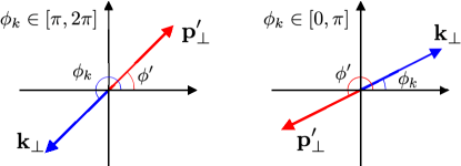
Figure 2: Two possible directions of the vectors $\mathbf{k}_{\perp}$ and $\mathbf{p}^{\prime}_{\perp}$ according to Eq.(55).

In what follows, we discuss the scheme with $\sigma_{\phi}\to 2\pi$ for simplicity for which the information about the electron momentum is incomplete, but the energy is well-defined, $\varepsilon^{\prime}=\sqrt{(p^{\prime}_{\perp})^{2}+(p^{\prime}_{z})^{2}+m_{e}^{2}}$. The corresponding amplitude is also obtained via the coherent averaging ($f=1$),

$$\int\limits_{0}^{2\pi}\frac{{\displaystyle d\phi^{\prime}}}{{\displaystyle 2\pi}}\,S_{fi}^{\rm(pw)}.$$ (52)

Formally, this expression coincides with (48) at $m^{\prime}-\lambda^{\prime}=0$, but its physical meaning is different. In the scheme (ii), we do measure the TAM projection and the helicity, and we can easily obtain $\langle\hat{L}_{z}\rangle=m^{\prime}-\lambda^{\prime}=0$, but during the generalized measurement we do not effectively measure the TAM at all, which implies projection to the state

$$|e^{\prime}_{\text{det}}\rangle^{\text{(g)}}=\int\limits_{0}^{2\pi}\frac{{\displaystyle d\phi^{\prime}}}{{\displaystyle 2\pi}}\,|{\bf p}^{\prime},\lambda^{\prime}\rangle,$$ (53)

where each plane wave enters with the same phase. The corresponding function $f_{p}({\bf p}^{\prime})$ from Eq.(35)

$$f_{p}({\bf p}^{\prime})=(2\pi)^{2}\delta\left(p^{\prime}_{z}-\langle p\rangle_{z}\right)\frac{1}{p^{\prime}_{\perp}}\delta\left(p^{\prime}_{\perp}-\langle p\rangle_{\perp}\right)$$ (54)

does not depend on the angle $\phi^{\prime}$ and it must be understood as a limiting case of a wave packet.

Working in cylindrical coordinates, we use the following representation (see Fig.2):

$$\delta({\bf p}^{\prime}_{\perp}+{\bf k}_{\perp})=\delta(p^{\prime}_{x}+k_{x})\delta(p^{\prime}_{y}+k_{y})=$$ (55)

$$\frac{{\displaystyle 1}}{{\displaystyle p^{\prime}_{\perp}}}\,\delta(p^{\prime}_{\perp}-k_{\perp})\left(\delta(\phi^{\prime}-(\phi_{k}-\pi))\Big{|}_{\phi_{k}\in[\pi,2\pi]}+\delta(\phi^{\prime}-(\phi_{k}+\pi))\Big{|}_{\phi_{k}\in[0,\pi]}\right).$$ (56)

Note that only one of these configurations contributes to the evolved state, and there is no interference between them (cf. Ref.[51, 8, 56]). Thus, in the simplest scheme with $\sigma_{\phi}\to 2\pi$ the evolved wave functions of the photon and of the fermion become

$${\bm{A}}^{(\text{ev})}_{(\text{g})}({\bf k},\omega)=\sum\limits_{\lambda_{\gamma}=\pm 1}{\bm{e}}\,\int\limits_{0}^{2\pi}\frac{{\displaystyle d\phi^{\prime}}}{{\displaystyle 2\pi}}\,S_{fi}^{(\text{pw})}\propto$$ (57)

$$\propto\int\frac{{\displaystyle d\phi^{\prime}}}{{\displaystyle 2\pi}}\,\delta({\bf p}^{\prime}_{\perp}+{\bf k}_{\perp})\propto\frac{{\displaystyle 1}}{{\displaystyle p^{\prime}_{\perp}}}\,\delta(p^{\prime}_{\perp}-k_{\perp}),$$ (58)

$$\psi^{(\text{ev})}_{(\text{g})}({\bf p}^{\prime},\varepsilon^{\prime})=\sum\limits_{\lambda^{\prime}=\pm 1/2}\,u^{\prime}\,\int\limits_{0}^{2\pi}\frac{{\displaystyle d\phi^{\prime}}}{{\displaystyle 2\pi}}\,S_{fi}^{(\text{pw})}.$$ (59)

where for the fermion the integration is performed over the azimuthal angle of the particle measured in the generalized scheme. The proportionality to $\delta(p^{\prime}_{\perp}-k_{\perp})$ instead of $\delta({\bf p}^{\prime}_{\perp}-{\bf k}_{\perp})$ is a hallmark of the Bessel state with the vanishing TAM-uncertainty. In Fig.3 we show one of the simplest examples how one can detect a charged particle scattered at a certain polar angle, but deliberately do not get any information about its azimuthal angle.

Finally, note that this generalized-measurement scenario can, somewhat surprisingly, guarantee the validity of the Bohr correspondence principle in the quasi-classical regime when the emitting particle experiences very small recoil and the scattering angle is vanishing, $\theta^{\prime}\ll 1$. For instance, in a number of processes, including Cherenkov radiation, synchrotron radiation, and the Compton effect, this angle can be of the order of

$$\theta^{\prime}\sim 10^{-6}-10^{-5}\,\text{rad}$$ (60)

for electrons and realistic parameters. Therefore, precise measurements of the angle $\phi^{\prime}$ can technically be very challenging at these small polar angles. This is the reason why predictions of this genuinely quantum generalized-measurement scheme provide coincidence with the classical theory.

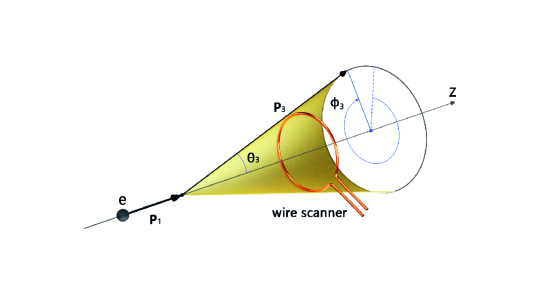
Figure 3: A ring-shaped wire scanner detects electrons scattered at a certain polar angle $\theta_{3}$, but does not measure the azimuthal angle $\phi_{3}$.

4 Example 1: Cherenkov radiation by a plane-wave or twisted electron

Consider Cherenkov emission,

$$e(p)\to e^{\prime}(p^{\prime})+\gamma(k),$$ (61)

in a transparent medium with weak frequency dispersion and a refractive index $\tilde{n}(\omega)$; see Fig.4 [80]. The incoming electron is described as a plane wave and the matrix element is

$$S_{fi}^{\rm(pw)}=-ieN(2\pi)^{4}\delta^{(4)}(p-p^{\prime}-k)\,\bar{u}^{\prime}\gamma^{\mu}u\,e^{*}_{\mu},$$ (62)

where $N$ is a normalization constant (see Ref.[50]) and

$$p=\{\varepsilon,0,0,|\bm{p}|\},\ p^{\prime}=\{\varepsilon^{\prime},p^{\prime}_{\perp}\cos\phi^{\prime},p^{\prime}_{\perp}\sin\phi^{\prime},p^{\prime}_{z}\},$$ (63)

$$p^{\prime}_{\perp}=|\bm{p}^{\prime}|\sin\theta^{\prime},\ k=\{\omega,k_{\perp}\cos\phi_{k},k_{\perp}\sin\phi_{k},k_{z}\},$$ (64)

$$|{\bf k}|=\sqrt{k_{\perp}^{2}+k_{z}^{2}}=\omega\,\tilde{n}(\omega),\,k_{\perp}=|{\bf k}|\sin\theta_{k}.$$ (65)

The phases are chosen so that the electron bispinors are eigenfunctions of the TAM z-projection operator with the eigenvalues $\lambda=\pm 1/2,\lambda^{\prime}=\pm 1/2$.

If the electron is detected in the above generalized-measurement scheme, we do not know the photon momentum azimuthal angle. Then, the photon evolved state becomes

$${\bm{A}}^{(\text{ev})}({\bf k},\omega)=\int\limits_{0}^{2\pi}\frac{{\displaystyle d\phi^{\prime}}}{{\displaystyle 2\pi}}\sum\limits_{\lambda_{\gamma}=\pm 1}{\bm{e}}\,S_{fi}^{\rm(pw)}=-ieN{\bm{n}}\times\left[{\bm{n}}\times\int\limits_{0}^{2\pi}\frac{{\displaystyle d\phi^{\prime}}}{{\displaystyle 2\pi}}(2\pi)^{4}\delta^{(4)}(p-p^{\prime}-k)\,\bar{u}^{\prime}{\bm{\gamma}}u\right],$$ (66)

where ${\bm{n}}={\bf k}/|{\bf k}|$, we employ the Coulomb gauge with $e^{\mu}=\{0,{\bm{e}}\}$, and the summation over the photon helicities is done with the following formula

$$\sum\limits_{\lambda_{\gamma}=\pm 1}e_{i}e^{*}_{j}=\delta_{ij}-n_{i}n_{j}.$$ (67)

Substituting Eq.(56) to Eq.(66), we arrive at (see technical details and notations in the Appendix B)

$${\bm{A}}^{(\text{ev})}=(-1)^{\lambda-\lambda^{\prime}}ieN(2\pi)^{3}\delta(\varepsilon-\varepsilon^{\prime}-\omega)\delta(|\bm{p}|-p_{z}^{\prime}-k_{z})\,\frac{{\displaystyle 1}}{{\displaystyle p^{\prime}_{\perp}}}\,\delta(p^{\prime}_{\perp}-k_{\perp})$$ (68)

$$\times\,\left(\sqrt{\varepsilon^{\prime}+m_{e}}\sqrt{\varepsilon-m_{e}}+2\lambda\,2\lambda^{\prime}\sqrt{\varepsilon+m_{e}}\sqrt{\varepsilon^{\prime}-m_{e}}\right)\left[\bm{F}-\bm{n}(\bm{n}\bm{F})\right],$$ (69)

where

$$\bm{F}=d_{\lambda\lambda^{\prime}}^{(1/2)}(\theta^{\prime})\,{\bm{\chi}}_{0}\,e^{i(\lambda-\lambda^{\prime})\phi_{k}}+\sqrt{2}\,d_{-\lambda\lambda^{\prime}}^{(1/2)}(\theta^{\prime})\,{\bm{\chi}}_{2\lambda}e^{-i(\lambda+\lambda^{\prime})\phi_{k}}.$$ (70)

Thus, the two terms with ${\bm{\chi}_{0}}\,e^{i(\lambda-\lambda^{\prime})\phi_{k}}$ and ${\bm{\chi}_{2\lambda}}\,e^{-i(\lambda+\lambda^{\prime})\phi_{k}}$ in $\bm{F}$ are eigenvectors of $\hat{s}_{z}$ operator with the eigenvalues $0$ and $2\lambda$, respectively, and the eigenfunctions of the OAM projection operator $\hat{L}_{z}=-i\partial/\partial\phi_{k}$ with the eigenvalues $\lambda-\lambda^{\prime}$ and $-\lambda-\lambda^{\prime}$, respectively. Therefore, the vector $\bm{F}$ itself is an eigenvector of the photon TAM projection operator $\hat{j}^{(\gamma)}_{z}=\hat{s}_{z}+\hat{L}_{z}$ with the eigenvalue $\lambda-\lambda^{\prime}$.

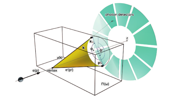
Figure 4: An azimuthal “which-way” experiment with Cherenkov radiation: during a projective measurement of the electron momentum ${\bf p}^{\prime}$ we learn the photon angle $\phi_{k}$, which is why the photon becomes a plane wave. However, if the electron angle $\phi^{\prime}$ is measured with a large error or is not measured at all, the angle $\phi_{k}$ stays undefined, and the photon evolved state automatically becomes twisted. In practice, the electron scattering angle is usually very small, $\theta^{\prime}\ll 1$, so precise measurements of the angle $\phi^{\prime}$ can be very challenging. In this quasi-classical regime the photons naturally become twisted being coherently emitted to all the azimuthal angles on the Cherenkov cone.

Similarly, using the representation

$${\bm{n}}=\sum\limits_{\sigma=0,\pm 1}d^{(1)}_{\sigma 0}(\theta_{k}){\bm{\chi}}_{\sigma}e^{-i\sigma\phi_{k}}$$ (71)

it is not difficult to prove that the vector $\bm{n}(\bm{n}\bm{F})$ and, therefore, the photon state $\bm{A}^{(\text{ev})}$ itself are eigenvectors of $\hat{j}^{(\gamma)}_{z}$ operator with a definite value of the photon TAM projection:

$$\hat{j}_{z}^{(\gamma)}\bm{A}^{(\text{ev})}=(\lambda-\lambda^{\prime})\bm{A}^{(\text{ev})},$$ (72)

where

$$\lambda-\lambda^{\prime}=\begin{cases}0,\ \text{if}\ \lambda^{\prime}=\lambda\ \text{(no electron TAM flip)},\\ 2\lambda=\pm 1,\ \lambda^{\prime}=-\lambda\ \text{(an electron TAM flip)}.\end{cases}$$ (73)

So, the maximum TAM value is $|j_{z}^{(\gamma)}|=1$. The transverse momentum $k_{\perp}$ of this Bessel beam equals to that of the final electron and, therefore, it can be written via the electron scattering angle $\theta^{\prime}$,

$$k_{\perp}=p^{\prime}_{\perp}=|\bm{p}^{\prime}|\sin\theta^{\prime}.$$ (74)

As this angle is usually negligibly small for Cherenkov radiation, $\theta^{\prime}\ll 1$, it is very challenging to precisely measure the azimuthal angle $\phi^{\prime}$. In this sense, Cherenkov radiation with no post-selection of $\phi^{\prime}$ can be viewed as a natural source of twisted photons, coherently emitted to all the azimuthal angles on the Cherenkov cone. We emphasize that even the state with the vanishing eigenvalue of $\hat{j}_{z}^{(\gamma)}$ operator in Eq.(69) is not a plane wave but a cylindrical one with the spin-orbit interaction (SOI).

Clearly, Eq.(73) simply represents the conservation law of the TAM $z$-projection $\hat{j}_{z}=\hat{j}^{\prime}_{z}+\hat{j}^{(\gamma)}_{z}$. Now recall that this conservation law takes place not only for the pure states with $\langle\hat{j}_{z}\rangle=\pm 1/2$, but also for the mixed states with $\langle\hat{j}_{z}\rangle\in[-1/2,1/2],\,\langle\hat{j}^{\prime}_{z}\rangle\in[-1/2,1/2]$. In the latter case, instead of Eq.(73) we have

$$\langle\hat{j}_{z}\rangle^{(\gamma)}=\langle\hat{j}_{z}\rangle-\langle\hat{j}^{\prime}_{z}\rangle,$$ (75)

where for the mixed electron states the photon TAM lies in the interval $\langle\hat{j}_{z}\rangle^{(\gamma)}\in[-1,1]$. In particular, when the initial electron is unpolarized, $\langle\hat{j}_{z}\rangle=0$, and the final electron TAM is not measured, $\langle\hat{j}^{\prime}_{z}\rangle=0$, the photon TAM is also vanishing, although it is not a plane wave.

Finally, when the initial electron is in a pure twisted state [33] with the TAM $z$-projection

$$m=\pm 1/2,\pm 3/2,...,$$ (76)

its bispinor $u\equiv u_{p\lambda}$ with $\bm{p}=\{p_{\perp}\cos\phi,p_{\perp}\sin\phi,p_{z}\}$ transforms as (see Eq. (44))

$$u_{p\lambda}\to u_{p_{\perp}p_{z}m\lambda}=i^{-(m-\lambda)}\int\limits_{0}^{2\pi}\frac{{\displaystyle d\phi}}{{\displaystyle 2\pi}}\,e^{i(m-\lambda)\phi}\,u_{p\lambda}.$$ (77)

The further integration over $\phi$ and $\phi^{\prime}$ can be performed analytically. As a result, the photon TAM transforms as $\lambda-\lambda^{\prime}\to m-\lambda^{\prime}$:

$$\hat{j}_{z}^{(\gamma)}\bm{A}^{(\text{ev})}=(m-\lambda^{\prime})\bm{A}^{(\text{ev})}.$$ (78)

Thus, vorticity of the incoming electron can be transferred to the photon within the generalized measurement scheme, and the twisted photons with the TAM $|j_{z}^{(\gamma)}|>1$ can be emitted. Clearly, the similar post-selection protocol can also be applied for other processes, including synchrotron radiation, transition radiation, diffraction radiation, Smith-Purcell radiation, and so on.

5 Example 2: non-linear Compton scattering
and undulator radiation

5.1 Post-selection to the plane-wave state

In a circularly polarized laser wave with the following potential [82, 94]

$$A^{\mu}=a_{1}^{\mu}\cos(kx)+a_{2}^{\mu}\sin(kx),$$ (79)

$$A^{2}=a_{1}^{2}=a_{2}^{2}=-a^{2}<0,$$ (80)

$$(a_{1}a_{2})=(ka_{1})=(ka_{2})=0,\ kx=\omega t-{\bf k}\cdot{\bf r}$$ (81)

an electron is conventionally described with a Volkov state [82, 94, 95, 96]

$$\psi_{p\lambda}({\bf r},t)=N_{e}\left(1+\frac{{\displaystyle e}}{{\displaystyle 2(pk)}}(\gamma k)(\gamma A)\right)\,u\,\exp\left\{-ipx-\frac{{\displaystyle ie}}{{\displaystyle(pk)}}\int\limits^{kx}d\varphi\left((pA)-\frac{{\displaystyle e}}{{\displaystyle 2}}A^{2}\right)\right\},$$ (82)

which is exact solution of the Dirac equation and where $\bar{u}u=2m_{e}$, $N_{e}$ is a normalization constant, and the second term in the pre-exponential factor is due to the spin,

$$(\gamma k)(\gamma A)=\frac{{\displaystyle 1}}{{\displaystyle 2}}\,\int\limits^{kx}d\varphi\,F^{\mu\nu}\sigma_{\mu\nu},$$ (83)

$$\sigma_{\mu\nu}=\frac{{\displaystyle 1}}{{\displaystyle 2}}\left(\gamma^{\mu}\gamma^{\nu}-\gamma^{\nu}\gamma^{\mu}\right),\ F^{\mu\nu}=\partial^{\mu}A^{\nu}-\partial^{\nu}A^{\mu}.$$ (84)

Note that the Volkov state (82) transforms into a plane wave when the laser field is off, $A\to 0$. The case when the incoming electron is twisted and is in a Bessel-Volkov state [44] is studied hereafter. The final photon wave function is also a plane wave,

$${\mathcal{A}}^{\mu}=N_{\gamma}\,e^{\prime\mu}\,e^{-i\omega^{\prime}t+i{\bf k}^{\prime}\cdot{\bf r}},\ k^{\prime}_{\mu}e^{\prime\mu}=0.$$ (85)

The corresponding matrix element is

$$S_{fi}^{(\text{pw})}=-ie\int d^{4}x\,\bar{\psi}_{p^{\prime}\lambda^{\prime}}\gamma_{\mu}\psi_{p\lambda}\left({\mathcal{A}}^{\mu}\right)^{*}$$ (86)

where the final electron is also in the Volkov state,

$$\bar{\psi}_{p^{\prime}\lambda^{\prime}}({\bf r},t)=N_{e^{\prime}}\,\bar{u}^{\prime}\,\left(1+\frac{{\displaystyle e}}{{\displaystyle 2(p^{\prime}k)}}(\gamma A)(\gamma k)\right)\,\exp\left\{ip^{\prime}x+\frac{{\displaystyle ie}}{{\displaystyle(p^{\prime}k)}}\int\limits^{kx}d\varphi\left((p^{\prime}A)-\frac{{\displaystyle e}}{{\displaystyle 2}}A^{2}\right)\right\}.$$ (87)

where $\bar{u}^{\prime}u^{\prime}=2m_{e}$.

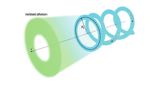
Figure 5: A schematic picture of emission of a photon during the motion of an electron wave packet along a helical path with a mean radius $\rho^{\prime}_{e}=ea/(p^{\prime}k)$, either in a helical undulator or in a circularly polarized laser wave. The evolved state of the photon becomes twisted only if the azimuthal angle of the emitting electron momentum is measured with a large error or is not measured at all, which is typical for the quasi-classical regime with the small scattering angle, $\theta^{\prime}\ll 1$. The radius of the first Bessel ring is of the order of $(p^{\prime}_{\perp})^{-1}$, which is usually larger than $\rho^{\prime}_{e}$ according to Eq.(141).

As this problem can be solved exactly [82, 94, 95, 96], its results can be applied for an approximate description of similar problems where an electron also moves along a helical path, the simplest example being emission in a helical undulator [97, 98, 99]. As shown, for instance, in Ref.[98], the spectral distributions of the radiated energy of both the processes are quantitatively very similar for ultrarelativistic electrons with $\varepsilon/m\gg 1$ and the small recoil $\omega^{\prime}/\varepsilon\ll 1$. We emphasize that although the electron is usually post-selected to the Volkov (plane-wave) state in calculations [82, 94, 95, 96], this implies a projective measurement of the electron quasi-momentum $q^{\prime}$ with the vanishing uncertainties of all its components (the scheme (i) from Sec.3.2).

Importantly, this may not necessarily happen in practice if we do not have complete information about the final electron state. Indeed, when the recoil is small and the electron scattering angle is vanishing, $\theta^{\prime}\ll 1$, the electron stays in the laser field or inside an undulator, its energy is thereby implicitly measured, but the momentum azimuthal angle may not be exactly known, simply because it is practically challenging to precisely measure it at the angles of $\theta^{\prime}\sim 10^{-6}-10^{-5}$ rad. Finally, inside a long undulator the number of emitted photons is large but the final electron azimuthal angle is not measured after each emission event at all. In this regime, the electron quasi-momentum is measured within the scheme (iii) from Sec.3.2, and the photon itself is automatically projected to the twisted state (see Fig.5). We will return to this generalized-measurement scheme in the next sub-section.

Following the standard procedure [82, 94, 95, 96], we expand the matrix element into series over the harmonic number $s\geqslant 1$, regroup the terms in the pre-exponential factor with the same indices of the Bessel functions $J_{s}$ and $J_{s\pm 1}$, and represent the result as follows:

$$S_{fi}^{(\text{pw})}=\sum\limits_{s=1}^{\infty}S_{fi}^{(s)}=-ieN\sum\limits_{s=1}^{\infty}(2\pi)^{4}\delta^{(4)}(q+sk-q^{\prime}-k^{\prime})\sum\limits_{\sigma=0,\pm 1}(e^{\prime}_{\mu})^{*}\,\bar{u}^{\prime}\,\Gamma_{\sigma}^{\mu}\,u\,J_{s+\sigma}(\Sigma)\,e^{i(s+\sigma)\xi}.$$ (88)

Here, $N=N_{e}N_{e^{\prime}}N_{\gamma}$ is a normalization constant, the electron quasi-momenta are

$$q^{\mu}=p^{\mu}+e^{2}\,k^{\mu}\frac{{\displaystyle a^{2}}}{{\displaystyle 2(pk)}},\,(q^{\prime})^{\mu}=(p^{\prime})^{\mu}+e^{2}\,k^{\mu}\frac{{\displaystyle a^{2}}}{{\displaystyle 2(p^{\prime}k)}},$$ (89)

and we have also denoted

$$\Sigma=e\sqrt{\left(\frac{{\displaystyle(pa_{1})}}{{\displaystyle(pk)}}-\frac{{\displaystyle(p^{\prime}a_{1})}}{{\displaystyle(p^{\prime}k)}}\right)^{2}+\left(\frac{{\displaystyle(pa_{2})}}{{\displaystyle(pk)}}-\frac{{\displaystyle(p^{\prime}a_{2})}}{{\displaystyle(p^{\prime}k)}}\right)^{2}},$$ (90)

$$\xi=\arctan\frac{{\displaystyle(pa_{2})/(pk)-(p^{\prime}a_{2})/(p^{\prime}k)}}{{\displaystyle(pa_{1})/(pk)-(p^{\prime}a_{1})/(p^{\prime}k)}}.$$ (91)

The “dressed” vertex $\Gamma_{\sigma}^{\mu}$ is

$$\Gamma_{\sigma}^{\mu}=\{\Gamma_{0}^{\mu},\Gamma_{+1}^{\mu},\Gamma_{-1}^{\mu}\}=$$ (92)

$$=\Big{\{}\gamma^{\mu}-k^{\mu}\frac{{\displaystyle e^{2}A^{2}}}{{\displaystyle 2(pk)(p^{\prime}k)}}(\gamma k),\frac{{\displaystyle 1}}{{\displaystyle 2}}(\gamma a_{-})\left(\frac{{\displaystyle e}}{{\displaystyle 2}}(\gamma k)\gamma^{\mu}(\frac{{\displaystyle 1}}{{\displaystyle(p^{\prime}k)}}-\frac{{\displaystyle 1}}{{\displaystyle(pk)}})+k^{\mu}\frac{{\displaystyle e}}{{\displaystyle(pk)}}\right)-a_{-}^{\mu}\frac{{\displaystyle e}}{{\displaystyle 2(pk)}}(\gamma k),$$ (93)

$$\frac{{\displaystyle 1}}{{\displaystyle 2}}(\gamma a_{+})\left(\frac{{\displaystyle e}}{{\displaystyle 2}}(\gamma k)\gamma^{\mu}(\frac{{\displaystyle 1}}{{\displaystyle(p^{\prime}k)}}-\frac{{\displaystyle 1}}{{\displaystyle(pk)}})+k^{\mu}\frac{{\displaystyle e}}{{\displaystyle(pk)}}\right)-a_{+}^{\mu}\frac{{\displaystyle e}}{{\displaystyle 2(pk)}}(\gamma k)\Big{\}},$$ (94)

$$a_{\pm}^{\mu}=a_{1}^{\mu}\pm ia_{2}^{\mu},(ka_{\pm})=0.$$ (95)

These expressions are still the standard ones [82, 94, 95, 96], just written differently.

In what follows, we only study the head-on collision, for which

$$p=\{\varepsilon,0,0,|{\bf p}|\},\ k=\{\omega,0,0,-\omega\},\ k^{\prime}=\{\omega^{\prime},k^{\prime}_{\perp}\cos\phi_{k^{\prime}},k^{\prime}_{\perp}\sin\phi_{k^{\prime}},k^{\prime}_{z}\},\,k^{\prime}_{\perp}=\omega^{\prime}\sin\theta_{k^{\prime}},$$ (96)

$$p^{\prime}=\{\varepsilon^{\prime},p^{\prime}_{\perp}\cos\phi^{\prime},p^{\prime}_{\perp}\sin\phi^{\prime},p^{\prime}_{z}\},\ p^{\prime}_{\perp}=|{\bf p}^{\prime}|\sin\theta^{\prime},$$ (97)

$$a_{1}^{\mu}=a\{0,1,0,0\},a_{2}^{\mu}=a\{0,0,1,0\},$$ (98)

$$a_{\pm}^{\mu}=a\{0,{\bm{e}}_{\pm}\},\ {\bm{e}}_{\pm}=\hat{{\bm{x}}}\pm i\hat{{\bm{y}}},\ \hat{{\bm{x}}}=\{1,0,0\},\ \hat{{\bm{y}}}=\{0,1,0\},$$ (99)

$$\delta^{(4)}(q+sk-q^{\prime}-k^{\prime})=\delta(q^{0}+s\omega-(q^{\prime})^{0}-\omega^{\prime})\delta(q_{z}+sk_{z}-q_{z}^{\prime}-k_{z}^{\prime})\delta^{(2)}({\bf p}^{\prime}_{\perp}+{\bf k}^{\prime}_{\perp}),$$ (100)

and the transverse delta-function can again be represented in cylindrical coordinates, see Eq.(56). In this case, $(pa_{1})=(pa_{2})=0$, the vertex $\Gamma_{\sigma}^{\mu}$ does not depend on the azimuthal angles of the final particles, and so

$$\tan\xi=\frac{{\displaystyle p_{y}^{\prime}}}{{\displaystyle p_{x}^{\prime}}}=\tan\phi^{\prime}\Rightarrow\xi=\phi^{\prime}+\pi q,\ q=0,1,2,...$$ (101)

For $q=0$, we have

$$\xi=\phi^{\prime}=\phi_{k^{\prime}}\pm\pi$$ (102)

due to the transverse delta-function. The argument of the Bessel functions becomes

$$\Sigma=\frac{{\displaystyle ea}}{{\displaystyle(p^{\prime}k)}}p^{\prime}_{\perp}=\frac{{\displaystyle ea}}{{\displaystyle(p^{\prime}k)}}k^{\prime}_{\perp}\equiv\rho^{\prime}_{e}k^{\prime}_{\perp},$$ (103)

where

$$\rho^{\prime}_{e}=\frac{{\displaystyle ea}}{{\displaystyle(p^{\prime}k)}}=\eta\,\frac{{\displaystyle m_{e}}}{{\displaystyle(p^{\prime}k)}}$$ (104)

is a classical radius of the final electron path (see the problem No.2 to Sec.47 in Ref.[100] and Fig.5) and

$$\eta=\frac{{\displaystyle e\sqrt{-A^{2}}}}{{\displaystyle m_{e}}}=\frac{{\displaystyle ea}}{{\displaystyle m_{e}}}$$ (105)

is a classical field strength parameter [82, 94, 95, 96]. Thus, the radius of the classical helical trajectory inside the laser wave naturally arises in the quantum theory. For an optical photon and a relativistic electron, we have roughly

$$\rho^{\prime}_{e}\sim\eta\,\lambda_{c}\,\frac{{\displaystyle m_{e}}}{{\displaystyle\varepsilon^{\prime}}}\frac{{\displaystyle m_{e}}}{{\displaystyle\omega}}\sim\frac{{\displaystyle\eta}}{{\displaystyle\gamma^{\prime}}}\times 0.1[\mu\text{m}],$$ (106)

$$\gamma^{\prime}=\varepsilon^{\prime}/m_{e},\ \lambda_{c}=1/m_{e},$$ (107)

which reaches the atomic scale,

$$\rho^{\prime}_{e}\sim 0.1\,\text{nm}-1\,\text{nm},$$ (108)

for $\gamma^{\prime}\sim 10-100,\eta\sim 0.1-1$.

Thus, the evolved state of the emitted photon (59) looks as follows:

$${\bm{A}}^{(\text{ev})}({\bf k}^{\prime},\omega^{\prime})=\sum\limits_{s=1}^{\infty}{\bm{A}}^{(\text{ev},s)}({\bf k}^{\prime},\omega^{\prime}),$$ (109)

$${\bf k}^{\prime}\cdot{\bm{A}}^{(\text{ev},s)}=0,\ {\bm{n}}^{\prime}={\bf k}^{\prime}/\omega^{\prime},$$ (110)

$${\bm{A}}^{(\text{ev},s)}({\bf k}^{\prime},\omega^{\prime})=-ieN(2\pi)^{4}\delta^{(4)}(q+sk-q^{\prime}-k^{\prime})$$ (111)

$$\times\sum\limits_{\lambda_{\gamma}=\pm 1}\sum\limits_{\sigma=0,\pm 1}{\bm{e}}^{\prime}e^{\prime*}_{\mu}\,\bar{u}^{\prime}\,\Gamma_{\sigma}^{\mu}\,u\,J_{s+\sigma}(\rho^{\prime}_{e}k^{\prime}_{\perp})\,e^{i(s+\sigma)\phi^{\prime}},$$ (112)

where the sum over $\sigma$ has appeared because of the spin terms (84). Summation over the photon helicities $\lambda_{\gamma}$ is done as in Eq.(67). Then, choosing the final electron bispinor as an eigenstate of $\hat{j}^{\prime}_{z}$ operator with the eigenvalue $\lambda^{\prime}=\pm 1/2$, as in Sec.B, the evolved state becomes

$${\bm{A}}^{(\text{ev},s)}({\bf k}^{\prime},\omega^{\prime})=-ieN(2\pi)^{4}\delta^{(4)}(q+sk-q^{\prime}-k^{\prime})$$ (113)

$$\times{\bm{n}}^{\prime}\times\left[{\bm{n}}^{\prime}\times\sum\limits_{\sigma^{\prime}=\pm 1/2}\sum\limits_{\sigma=0,\pm 1}d^{(1/2)}_{\sigma^{\prime}\lambda^{\prime}}(\theta^{\prime})\,\bar{u}_{\varepsilon^{\prime}\lambda^{\prime}}^{(\sigma^{\prime})}\,{\bm{\Gamma}}_{\sigma}\,u\,J_{s+\sigma}(\rho^{\prime}_{e}k^{\prime}_{\perp})\,e^{i(s+\sigma+\sigma^{\prime}-\lambda^{\prime})\phi^{\prime}}\right].$$ (114)

where we have expanded the final electron bispinor according to Eq.(192). Clearly, this wave function is just a plane wave with the vanishing $z$-projection of the OAM because the photon has the definite 4-momentum $k^{\prime}$ and the azimuthal angle $\phi_{k^{\prime}}$.

5.2 Post-selection with a generalized measurement

5.2.1 Volkov electron

In the standard projective-measurement scheme, we detect photons emitted in a laser wave or in a helical undulator with a detector placed at an angle $\phi_{k^{\prime}}$, which automatically projects the electron to the plane-wave (Volkov) state $|{\bm{q}}^{\prime},\lambda^{\prime}\rangle$ with $\phi^{\prime}=\phi_{k^{\prime}}\pm\pi$. However, if we do not measure the electron angle $\phi^{\prime}$ alone, as we argued above, then the photon itself evolves to the twisted state, irrespectively of what detector is subsequently used. The electron detected state in the generalized-measurement scheme with the maximized error is

$$|e^{\prime}_{\text{det}}\rangle^{(\text{g})}=\int\limits_{0}^{2\pi}\frac{{\displaystyle d\phi^{\prime}}}{{\displaystyle 2\pi}}\,|{\bm{q}}^{\prime},\lambda^{\prime}\rangle,$$ (115)

and the information about the electron quasi-momentum ${\bm{q}}^{\prime}$ is incomplete. Importantly, in the head-on geometry (100) we have ${\bf p}^{\prime}_{\perp}={\bm{q}}^{\prime}_{\perp}$, and so the azimuthal angles of both the vectors coincide.

We can obtain the evolved photon wave function by integrating Eq.(114)

$${\bm{A}}^{(\text{ev},s)}_{(\text{g})}({\bf k}^{\prime},\omega^{\prime})=\int\limits_{0}^{2\pi}\frac{{\displaystyle d\phi^{\prime}}}{{\displaystyle 2\pi}}\,{\bm{A}}^{(\text{ev},s)}({\bf k}^{\prime},\omega^{\prime})=$$ (116)

$$=-ieN(2\pi)^{3}\delta(q^{0}+s\omega-(q^{\prime})^{0}-\omega^{\prime})\delta(q_{z}+sk_{z}-q_{z}^{\prime}-k_{z}^{\prime})\,\frac{{\displaystyle 1}}{{\displaystyle k_{\perp}^{\prime}}}\delta(p_{\perp}^{\prime}-k_{\perp}^{\prime})$$ (117)

$$\times{\bm{n}}^{\prime}\times\left[{\bm{n}}^{\prime}\times\sum\limits_{\sigma^{\prime}=\pm 1/2}\sum\limits_{\sigma=0,\pm 1}d^{(1/2)}_{\sigma^{\prime}\lambda^{\prime}}(\theta^{\prime})\,\bar{u}_{\varepsilon^{\prime}\lambda^{\prime}}^{(\sigma^{\prime})}\,{\bm{\Gamma}}_{\sigma}\,u\,J_{s+\sigma}(\rho^{\prime}_{e}k^{\prime}_{\perp})\,e^{i(s+\sigma+\sigma^{\prime}-\lambda^{\prime})(\phi_{k^{\prime}}\pm\pi)}\right].$$ (118)

Even without the calculation of $\bar{u}_{\varepsilon^{\prime}\lambda^{\prime}}^{(\sigma^{\prime})}\,{\bm{\Gamma}}_{\sigma}\,u$, it is now clear that the photon represents a cylindrical wave with the SOI.

Next, we use the representation

$$\bar{u}_{\varepsilon^{\prime}\lambda^{\prime}}^{(\sigma^{\prime})}\,{\bm{\Gamma}}_{\sigma}\,u={\bm{G}}^{(\uparrow\uparrow)}\,\delta_{\lambda,\sigma^{\prime}}+{\bm{G}}^{(\uparrow\downarrow)}\,\delta_{\lambda,-\sigma^{\prime}},$$ (119)

where the vectors ${\bm{G}}^{(\uparrow\uparrow)}\equiv{\bm{G}}^{(\uparrow\uparrow)}_{\sigma\lambda^{\prime}\lambda},{\bm{G}}^{(\uparrow\downarrow)}\equiv{\bm{G}}^{(\uparrow\downarrow)}_{\sigma\lambda^{\prime}\lambda}$ are found as

$${\bm{G}}^{(\uparrow\uparrow)}_{0\lambda^{\prime}\lambda}={\bm{\chi}}_{0}\left(f^{(2)}_{\lambda^{\prime}\lambda}-\frac{{\displaystyle\eta^{2}m_{e}^{2}\omega^{2}}}{{\displaystyle 2(pk)(p^{\prime}k)}}(f^{(1)}_{\lambda^{\prime}\lambda}+f^{(2)}_{\lambda^{\prime}\lambda})\right),$$ (120)

$${\bm{G}}^{(\uparrow\downarrow)}_{0\lambda^{\prime}\lambda}=-f^{(2)}_{\lambda^{\prime}\lambda}\sqrt{2}\,{\bm{\chi}}_{2\lambda},$$ (121)

$${\bm{G}}^{(\uparrow\uparrow)}_{\pm 1\lambda^{\prime}\lambda}=\mp\sqrt{2}\,{\bm{\chi}}_{\mp 1}\frac{{\displaystyle\eta m_{e}\omega}}{{\displaystyle 2}}\left(f^{(1)}_{\lambda^{\prime}\lambda}+f^{(2)}_{\lambda^{\prime}\lambda}\right)\left(\delta_{\lambda,\mp 1/2}\left(\frac{{\displaystyle 1}}{{\displaystyle(p^{\prime}k)}}-\frac{{\displaystyle 1}}{{\displaystyle(pk)}}\right)+\frac{{\displaystyle 1}}{{\displaystyle(pk)}}\right),$$ (122)

$${\bm{G}}^{(\uparrow\downarrow)}_{\pm 1\lambda^{\prime}\lambda}=\mp{\bm{\chi}}_{0}\frac{{\displaystyle\eta m_{e}\omega}}{{\displaystyle 2}}\delta_{\lambda,\pm 1/2}\left(\left(\frac{{\displaystyle 1}}{{\displaystyle(p^{\prime}k)}}-\frac{{\displaystyle 1}}{{\displaystyle(pk)}}\right)(f^{(1)}_{\lambda^{\prime}\lambda}-f^{(2)}_{\lambda^{\prime}\lambda})-\frac{{\displaystyle 2f^{(2)}_{\lambda^{\prime}\lambda}}}{{\displaystyle(pk)}}\right),$$ (123)

$$f^{(1)}_{\lambda^{\prime}\lambda}=\sqrt{\varepsilon+m_{e}}\sqrt{\varepsilon^{\prime}+m_{e}}+2\lambda 2\lambda^{\prime}\sqrt{\varepsilon-m_{e}}\sqrt{\varepsilon^{\prime}-m_{e}},$$ (124)

$$f^{(2)}_{\lambda^{\prime}\lambda}=\sqrt{\varepsilon-m_{e}}\sqrt{\varepsilon^{\prime}+m_{e}}+2\lambda 2\lambda^{\prime}\sqrt{\varepsilon+m_{e}}\sqrt{\varepsilon^{\prime}-m_{e}},$$ (125)

and they do not explicitly depend on the photon 4-momentum $k^{\prime}$. The vectors ${\bm{\chi}}_{0},{\bm{\chi}}_{\pm 1}$ are given in Eq.(202). The final expression for the wave function is

$${\bm{A}}^{(\text{ev},s)}_{(\text{g})}({\bf k}^{\prime},\omega^{\prime})=-ie(-1)^{s+\lambda-\lambda^{\prime}}N(2\pi)^{3}\delta(q^{0}+s\omega-(q^{\prime})^{0}-\omega^{\prime})\delta(q_{z}+sk_{z}-q_{z}^{\prime}-k_{z}^{\prime})\,\frac{{\displaystyle 1}}{{\displaystyle k_{\perp}^{\prime}}}\delta(p_{\perp}^{\prime}-k_{\perp}^{\prime})$$ (126)

$$\times{\bm{n}}^{\prime}\times\left[{\bm{n}}^{\prime}\times\sum\limits_{\sigma=0,\pm 1}J_{s+\sigma}(\rho^{\prime}_{e}k^{\prime}_{\perp})\,e^{i(s+\sigma-\lambda^{\prime})\phi_{k^{\prime}}}\left(d^{(1/2)}_{\lambda\lambda^{\prime}}(\theta^{\prime})\,{\bm{G}}_{\sigma\lambda^{\prime}\lambda}^{(\uparrow\uparrow)}\,e^{i\lambda\phi_{k^{\prime}}}+d^{(1/2)}_{-\lambda\lambda^{\prime}}(\theta^{\prime})\,{\bm{G}}_{\sigma\lambda^{\prime}\lambda}^{(\uparrow\downarrow)}\,e^{-i\lambda\phi_{k^{\prime}}}\right)\right],$$ (127)

which is a Bessel beam with the SOI, revealed by the sum over $\sigma$, and the following TAM projection:

$$\hat{j}_{z}^{(\gamma)}{\bm{A}}^{(\text{ev},s)}_{(\text{g})}=(s+\lambda-\lambda^{\prime}){\bm{A}}^{(\text{ev},s)}_{(\text{g})},$$ (128)

whereas the TAM uncertainty is vanishing. Here, in contrast to Eq.(73) for Cherenkov radiation, the harmonic number $s=1,2,3,...$ appears in the r.h.s. For the unpolarized electrons with $\langle\hat{j}_{z}\rangle=\langle\hat{j}^{\prime}_{z}\rangle=0$, the photon TAM is simply $s$. Analogously to Cherenkov radiation, the transverse momentum of this Bessel photon is defined by the electron scattering angle $\theta^{\prime}$ as

$$k^{\prime}_{\perp}=|{\bf p}^{\prime}|\sin\theta^{\prime}.$$ (129)

As argued in Sec.2, the coordinate representation for 1-particle evolved states has a clear interpretation only when the other particle wave-packet is localized spatially and temporarily, and so the electron detector function $f_{p}$ is smooth. Nevertheless – even without such a localization – the monochromatic Bessel beam in the coordinate representation

$$\displaystyle{\bm{A}}^{({\text{ev}},s)}_{(\text{g})}({\bf r},t)=\int\frac{d^{3}k^{\prime}}{(2\pi)^{3}}\,\frac{1}{\sqrt{2\omega^{\prime}}}\,{\bm{A}}^{(\text{ev}),s}_{(\text{g})}({\bf k}^{\prime},\omega^{\prime})\,e^{-i\omega^{\prime}t+i{\bf k}^{\prime}\cdot{\bf r}}$$ (130)

can be used to visualize spatial distribution of the emitted energy. To this end, it is convenient to divide the vector potential (127) into the following parts:

$${\bm{A}}^{({\text{ev}},s)}_{(\text{g})}\equiv{\bm{A}}^{({\text{ev}},s)}_{\bm{G}}+{\bm{A}}^{({\text{ev}},s)}_{{\bm{n}}^{\prime}},$$ (131)

$${\bm{A}}^{({\text{ev}},s)}_{\bm{G}}\propto{\bm{G}},\ {\bm{A}}^{({\text{ev}},s)}_{{\bm{n}}^{\prime}}\propto{\bm{n}}^{\prime}({\bm{n}}^{\prime}\cdot{\bm{G}}),$$ (132)

where ${\bm{G}}$ is either ${\bm{G}}_{\sigma\lambda^{\prime}\lambda}^{(\uparrow\uparrow)}$ or ${\bm{G}}_{\sigma\lambda^{\prime}\lambda}^{(\uparrow\downarrow)}$. For the former part, we obtain

$$\displaystyle{\bm{A}}^{({\text{ev}},s)}_{\bm{G}}({\bf r},t)=ie(-1)^{s+\lambda-\lambda^{\prime}}N\,\frac{2\pi}{\sqrt{2\omega^{\prime}}}\,\delta(q^{0}+s\omega-(q^{\prime})^{0}-\omega^{\prime})\,e^{-it(q^{0}+s\omega-(q^{\prime})^{0})+iz(q_{z}+sk_{z}-q_{z}^{\prime})}$$ (133)

$$\times\sum\limits_{\sigma=0,\pm 1}i^{s+\sigma-\lambda^{\prime}}\,J_{s+\sigma}(\rho^{\prime}_{e}p^{\prime}_{\perp})\,e^{i(s+\sigma-\lambda^{\prime})\phi_{r}}\Big{(}i^{\lambda}\,d^{(1/2)}_{\lambda\lambda^{\prime}}(\theta^{\prime})\,{\bm{G}}_{\sigma\lambda^{\prime}\lambda}^{(\uparrow\uparrow)}\,e^{i\lambda\phi_{r}}\,J_{s+\sigma-\lambda^{\prime}+\lambda}(\rho p^{\prime}_{\perp})+$$ (134)

$$+i^{-\lambda}d^{(1/2)}_{-\lambda\lambda^{\prime}}(\theta^{\prime})\,{\bm{G}}_{\sigma\lambda^{\prime}\lambda}^{(\uparrow\downarrow)}\,e^{-i\lambda\phi_{r}}J_{s+\sigma-\lambda^{\prime}-\lambda}(\rho p^{\prime}_{\perp})\Big{)},$$ (135)

where $\omega^{\prime}=q^{0}+s\omega-(q^{\prime})^{0}=\sqrt{(p^{\prime}_{\perp})^{2}+(q_{z}+sk_{z}-q_{z}^{\prime})^{2}}$ and $\phi_{r}$ is the azimuthal angle of the vector

$${\bf r}=\{\rho\cos\phi_{r},\rho\sin\phi_{r},z\},$$ (136)

and the following identity has been used

$$\int\limits_{0}^{2\pi}\frac{d\phi}{2\pi}\,e^{ix\cos\phi+i\ell\phi}=i^{\ell}J_{\ell}(x).$$ (137)

Clearly, the part ${\bm{A}}^{({\text{ev}},s)}_{{\bm{n}}^{\prime}}({\bf r},t)$ is much more cumbersome.

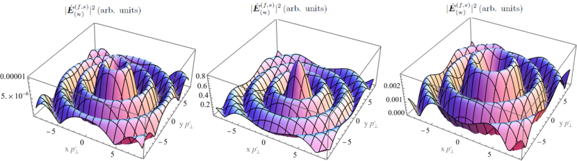
Figure 6: The regularized spatial energy distributions (138) of the Bessel photon emitted in the non-linear Compton scattering within the generalized-measurement scheme (iii) with the electron azimuthal angle being measured with a very large error or not measured at all. Left panel: $\omega=5\,\text{eV},\,\varepsilon/m_{e}=10,\varepsilon^{\prime}=0.9999\,\varepsilon,\theta^{\prime}\approx 10^{-5}\,\text{rad},\eta=0.5,s=1,\lambda=-1/2,\lambda^{\prime}=1/2$ (a spin flip), $j_{z}^{(\gamma)}=s+\lambda-\lambda^{\prime}=0$. Central panel: the same, but $\lambda=1/2,\lambda^{\prime}=1/2$ (no spin flip), $j_{z}^{(\gamma)}=s+\lambda-\lambda^{\prime}=1$. Right panel: $\omega=0.5\,\text{eV},\,\varepsilon/m_{e}=100,\varepsilon^{\prime}=0.9999\,\varepsilon,\theta^{\prime}\approx 10^{-6}\,\text{rad},\eta=0.5,s=3,\lambda=1/2,\lambda^{\prime}=1/2$ (no spin flip), $j_{z}^{(\gamma)}=s+\lambda-\lambda^{\prime}=3$. Everywhere $(p^{\prime}_{\perp})^{-1}\approx 4\,\text{nm}\approx 4\rho^{\prime}_{e}$, so the Bessel rings are wider than the radius of the electron classical path $\rho^{\prime}_{e}$ (104) according to Eq.(141).

The electric field strength is ${\bm{E}}_{(\text{g})}^{({\text{ev}},s)}({\bf r},t)=-\partial{\bm{A}}^{({\text{ev}},s)}_{(\text{g})}({\bf r},t)/\partial t$, and the regularized spatial distributions of the energy of this Bessel beam

$$|\dot{{\bm{E}}}_{(\text{g})}^{({\text{ev}},s)}|^{2}=\frac{1}{T}\,\int d\omega^{\prime}|{\bm{E}}_{(\text{g})}^{({\text{ev}},s)}({\bf r},t)|^{2}$$ (138)

represent a typical doughnut, as shown in Fig.6. Here $T$ is a very large “observation time” obtained when squaring the delta-function in Eq.(135) (see, e.g., [82]). Importantly, whereas the radius of the emitting electron classical path (104) does not change much during the emission of soft photons, $\rho^{\prime}_{e}\approx\rho_{e}$, the radius of the first Bessel ring is of the order of $1/p^{\prime}_{\perp}\approx 1/\varepsilon^{\prime}\theta^{\prime}$, which does not necessarily coincide with $\rho_{e}$. Indeed, the electron scattering angle is usually small and limited from above [101],

$$\displaystyle\theta^{\prime}\leq\frac{2s}{\sqrt{1+\eta^{2}}}\,\frac{\omega}{m_{e}},$$ (139)

so the photon transverse momentum is

$$\displaystyle k^{\prime}_{\perp}\leq\varepsilon^{\prime}\,\frac{2s}{\sqrt{1+\eta^{2}}}\,\frac{\omega}{m_{e}},$$ (140)

and it can reach the keV scale for GeV electrons and optical laser photons. Detailed study of the quasi-classical regime of emission by ultrarelativistic electrons is presented in the Appendix, Sec.C, and comparison with the predictions of classical electrodynamics are given in the Appendix, Sec.D. That is why in the relativistic case we have

$$\displaystyle\frac{(p^{\prime}_{\perp})^{-1}}{\rho^{\prime}_{e}}\approx\frac{2}{\eta}\frac{\omega}{m_{e}}\frac{1}{\theta^{\prime}}\geq\frac{\sqrt{1+\eta^{2}}}{s\,\eta}.$$ (141)

Very roughly, one can think of $(k^{\prime}_{\perp})^{-1}=(p^{\prime}_{\perp})^{-1}$ as of the transverse coherence length of the twisted photon, although this quantity cannot be quantitatively defined for an unnormalized Bessel beam. Thus, in the linear regime with $\eta\ll 1$ the radius of the first Bessel ring is much larger than the radius of the electron classical path, while in the non-linear regime with $\eta\gtrsim 1$ this ratio is of the order of unity, as shown in Fig.5. The opposite case with $\eta\gg 1$ corresponds to a constant crossed field instead of the plane wave [82, 94], and the above ratio gets larger than $1/s$.

5.2.2 Bessel-Volkov electron

Let us now turn to the case when the incoming electron is twisted with the TAM $m=\pm 1/2,3/2,...$ and it is in the Bessel-Volkov state [44]. Clearly, this time we obtain

$$\hat{j}_{z}^{(\gamma)}{\bm{A}}^{(f,s)}_{(\text{g})}=(s+m-\lambda^{\prime}){\bm{A}}^{(f,s)}_{(\text{g})},$$ (142)

whereas the most general formula for the mixed states is

$$\langle\hat{j}_{z}\rangle^{(\gamma)}=s+\langle\hat{j}_{z}\rangle-\langle\hat{j}^{\prime}_{z}\rangle.$$ (143)

Thus, highly twisted photons with $\langle\hat{j}_{z}^{(\gamma)}\rangle\gg 1$ can be obtained via the non-linear Compton effect

• Either by using the plane-wave (Volkov) incoming electrons and a powerful laser with $\eta\gtrsim 1$, so that the higher harmonics with $s>1$ are generated,

• Or, alternatively, by taking a moderately powerful laser, for which only the linear scattering with $s=1$ takes place, but with an incoming vortex (Bessel-Volkov) electron with $|m|\gg 1$.

As the highly twisted electrons with $m\sim 100-1000$ have already been obtained [33], the latter scheme seems to be technically easier. Besides, if the vortex electron is ultrarelativistic, the energy of the scattered highly twisted photons can easily reach MeV range [6]. The means for accelerating the vortex electrons to ultrarelativistic energies have been recently discussed in Ref.[66].

We emphasize that in the quantum regime the twisted photons are not naturally generated in a circularly-polarized laser wave or in a helical undulator, as it seems from the classical theory [13, 14, 15, 22, 23, 24]. In quantum approach, the photon turns out to be twisted only if the measurement error of the azimuthal angle of the final electron momentum is large. When the recoil angle $\theta^{\prime}$ is small, the angle $\phi^{\prime}$ simply loses its sense, which is why this generalized-measurement scheme reproduces results of the classical theory.

6 Example 3: Heavy and composite particles

6.1 Leptons

An advantage of the generalized-measurement technique is that it can in principle be applied to particles of any mass, spin, and energy, including composite particles. We start with the QED scattering with a lepton heavier than electron,

$$e^{\pm}\mu^{\pm}\to e^{\pm}\mu^{\pm}\quad\text{or}\quad e^{\pm}\tau^{\pm}\to e^{\pm}\tau^{\pm}.$$ (144)

For definiteness we take the process

$$e^{-}(p_{1})+\mu^{-}(p_{2})\to e^{-}(p_{3})+\mu^{-}(p_{4})$$ (145)

as an example, where the electron and the muon collide head-on and have the momenta

$$p_{1}=\{\varepsilon_{1},0,0,|\bm{p}_{1}|\},\,\varepsilon_{1}=\sqrt{m_{e}^{2}+|\bm{p}_{1}|^{2}},$$ (146)

$$\text{and}\quad p_{2}=\{\varepsilon_{2},0,0,-|\bm{p}_{2}|\},\,\varepsilon_{2}=\sqrt{m_{\mu}^{2}+|\bm{p}_{2}|^{2}},$$ (147)

as well as the helicities $\lambda_{1},\lambda_{2}$, respectively. When the final electron is detected in the generalized-measurement scheme, the evolved wave function of the muon, according to Eq.(59), becomes

$$\psi^{(f)}_{\mu}=\sum\limits_{\lambda_{4}=\pm 1/2}\int\limits_{0}^{2\pi}\frac{{\displaystyle d\phi_{3}}}{{\displaystyle 2\pi}}\,u_{4}\,S_{fi}^{\rm(pw)},$$ (148)

where $u_{4}\equiv u_{p_{4}\lambda_{4}}$ and the matrix element reads

$$S_{fi}^{\rm(pw)}=i(2\pi)^{4}N\,\delta^{(4)}(p_{1}+p_{2}-p_{3}-p_{4})$$ (149)

$$\times\frac{{\displaystyle 4\pi e^{2}}}{{\displaystyle q^{2}}}\,\left(\bar{u}_{3}\gamma^{\alpha}u_{1}\right)\,\left(\bar{u}_{4}\gamma_{\alpha}u_{2}\right),\,q=p_{1}-p_{3},$$ (150)

where the photon propagator is taken in the Feynman gauge. In contrast to the previous section, the 4-vector $q$ is a momentum transfer.

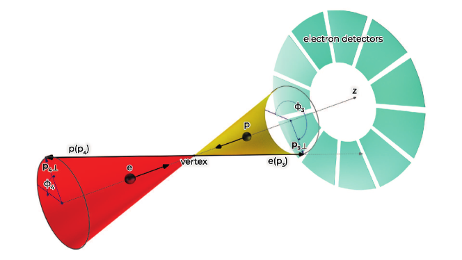
Figure 7: An azimuthal “which-way” experiment with elastic $ep\to ep$ scattering. The evolved state of the proton becomes twisted if the electron azimuthal angle $\phi_{3}$ is measured with a large error or not measured at all. The same scheme can also be applied to elastic and inelastic processes with other hadrons, ions, and nuclei.

The muon current can be presented as

$$\bar{u}_{4}\gamma_{\alpha}u_{2}=J^{(\mu)}_{\alpha}e^{-i(\lambda_{2}+\lambda_{4})\phi_{4}},$$ (151)

where $J^{(\mu)}_{\alpha}$ is given in Eq.(207) of the Appendix B with $m_{e}\to m_{\mu}$. After the integration, the electron current becomes

$$\int\limits_{0}^{2\pi}d\phi_{3}\,\delta(\phi_{3}-(\phi_{4}\pm\pi))\,\bar{u}_{3}\gamma_{\alpha}u_{1}=$$ (152)

$$=J^{(e)}_{\alpha}(\phi_{3}=\phi_{4}\pm\pi)e^{i(\lambda_{1}-\lambda_{3})(\phi_{4}\pm\pi)}.$$ (153)

Taking into account that

$${\bm{\chi}}_{-2\lambda_{2}}\cdot{\bm{\chi}}_{2\lambda_{1}}=-\delta_{\lambda_{2}\lambda_{1}},$$ (154)

it is easy to check that the scalar product

$$\mathcal{J}\equiv J_{\alpha}^{(e)}(\phi_{3}=\phi_{4}\pm\pi)\,(J^{(\mu)})^{\alpha}$$ (155)

does not depend on $\phi_{4}$. Therefore,

$$\psi^{(f)}_{\mu}\propto\sum\limits_{\lambda_{4}=\pm 1/2}\tilde{u}_{4}\,\,\mathcal{J}\,e^{i(\lambda_{1}-\lambda_{2}-\lambda_{3})\phi_{4}},$$ (156)

where $\tilde{u}_{4}=u_{4}\,e^{-i\lambda_{4}\phi_{4}}$ has a vanishing TAM, see Eq.(189) in the Appendix B. As a result,

$${\hat{j}}_{4,z}\psi^{(f)}_{\mu}=(\lambda_{1}-\lambda_{2}-\lambda_{3})\psi^{(f)}_{\mu},$$ (157)

i.e. the muon becomes twisted.

Similarly, for the twisted incoming electron with $m=\pm 1/2,3/2,\ldots$, the TAM of the final muon becomes

$$j_{4,z}=m-\lambda_{2}-\lambda_{3}.$$ (158)

Dealing with the unpolarized initial muon and the final electron, the incoming electron TAM $m$ is simply transferred to the muon,

$$\langle\hat{j}_{z}\rangle^{(\mu)}=m.$$ (159)

Clearly, the same TAM-transfer can be realized in other processes like $e^{-}e^{+}\leftrightarrow 2\gamma,e^{-}e^{+}\to\tau^{-}\tau^{+}$, etc. For instance, it has been recently shown in Ref. [60] that a hallmark of the muon’s twisted state is the modification of the electron spectra as the incoming muon decays into an electron and two neutrinos. Such a modification can be experimentally observed, which would prove the vortex state of the muon.

6.2 Hadrons

Finally, we study scattering off a hadron taking as an example elastic scattering of an electron by a proton with a mass $m_{p}$,

$$e(p_{1})+p(p_{2})\to e(p_{3})+p(p_{4}),$$ (160)

in the same head-on geometry (see Fig.7 [80]) with $p_{3}=\{\varepsilon_{3},p_{3,\perp}\cos\phi_{3},p_{3,\perp}\sin\phi_{3},p_{3,z}\}$ and similarly for $p_{4}$. Generalization to other hadrons, ions, nuclei, or to the inelastic processes due to the non-electromagnetic forces (say, to deep-inelastic $ep$ or $p\bar{p}$ scattering) is straightforward.

The plane-wave matrix element reads

$$S_{fi}^{\rm(pw)}=i(2\pi)^{4}N\,\delta^{(4)}(p_{1}+p_{2}-p_{3}-p_{4})$$ (161)

$$\times\frac{{\displaystyle 4\pi e^{2}}}{{\displaystyle q^{2}}}\,\left(\bar{u}_{3}\gamma^{\mu}u_{1}\right)\,\left(\bar{u}_{4}\Gamma_{\mu}u_{2}\right),$$ (162)

where

$$\Gamma_{\mu}=F_{1}\,\gamma_{\mu}+F_{2}\,\sigma_{\mu\nu}q^{\nu}$$ (163)

is a hadronic vertex, parametrized with two form-factors [82, 83]

$$F_{1}=F_{1}(q^{2},P^{2}),F_{2}=F_{2}(q^{2},P^{2}),$$ (164)

where

$$q^{2}=(p_{1}-p_{3})^{2},\,P^{2}=(p_{4}+p_{2})^{2}/4$$ (165)

do not depend on the angle $\phi_{4}$ of the final proton. So the form-factors do not depend on it either. Here also

$$\sigma^{\mu\nu}=\frac{1}{2}(\gamma^{\mu}\gamma^{\nu}-\gamma^{\nu}\gamma^{\mu})=({\bm{\alpha}},i{\bm{\Sigma}}),$$ (166)

where ${\bm{\alpha}},{\bm{\Sigma}}$ are the $4\times 4$ Dirac matrices in the standard representation [82].

First, one can prove that

$$\bar{u}_{3}(\phi_{3}=\phi_{4}\pm\pi)\gamma^{\mu}u_{1}\,\left(\bar{u}_{4}\Gamma_{\mu}u_{2}\right)\propto e^{i(\lambda_{1}-\lambda_{2}-\lambda_{3}-\lambda_{4})\phi_{4}},$$ (167)

and then we use Eq.(216) from the Appendix B for $\sigma^{\mu\nu}q_{\nu}$. The evolved wave function of the final proton is defined by Eq.(59),

$$\displaystyle\psi^{(f)}_{p}=\sum\limits_{\lambda_{4}=\pm 1/2}\int\limits_{0}^{2\pi}\frac{{\displaystyle d\phi_{3}}}{{\displaystyle 2\pi}}\,u_{4}\,S_{fi}^{(pw)}$$ (168)

Within the same generalized-measurement protocol (see Fig.7), the evolved wave function of the proton becomes twisted,

$$\hat{j}_{4,z}\psi^{(f)}_{p}=(\lambda_{1}-\lambda_{2}-\lambda_{3})\,\psi^{(f)}_{p}.$$ (169)

When the incoming electron is twisted with the TAM z-projection $m$, we have

$$\lambda_{1}-\lambda_{2}-\lambda_{3}\to m-\lambda_{2}-\lambda_{3}$$ (170)

If the initial hadron is unpolarized and the electron polarization is not measured, the electron TAM is transferred to the hadron,

$$\langle\hat{j}_{z}\rangle^{(p)}=m.$$ (171)

Clearly, this TAM transfer can also be realized for other particles, regardless of their masses and spins, including neutrons, pions, atoms, ions, and nuclei.

7 Discussion and conclusion

We have theoretically demonstrated that quantum entanglement in a pair of particles together with the generalized measurement on one of them can be employed for generating a highly energetic vortex state of the other – in principle arbitrary – particle. We have given examples when the measurement error is maximized and the resultant vortex states represent the Bessel beams of photons, electrons, muons, hadrons, etc. Were this error smaller, $\sigma_{\phi}<2\pi$, the resultant states would be the Bessel-like wave packets with a finite uncertainty of the angular momentum but with the same central value, defined by the TAM conservation law.

Somewhat surprisingly, it is this inherently quantum approach with the large measurement error that most adequately describes the emission of twisted photons when the recoil is vanishing, thus providing agreement with the classical theory. More importantly, the developed model explicitly demonstrates that it is the measurement protocol that can guarantee vorticity of a final particle, whereas helical motion of the charged particles alone (say, during the heavy-ion collisions [63]) does not automatically lead to the twisted state of the resultant particles. Indeed, even during quantum transitions between the different Landau levels of a charged particle in magnetic field the emitted photon is not always twisted [104].

The transverse momentum of the resultant twisted particle is defined by that of the other particle whose azimuthal angle is measured with a large error. Thus, selecting the particles scattered at larger polar angles – say, in $ep,\gamma e,\gamma p$, $\gamma$-ion, or ion-ion collisions – one can in principle obtain the vortex beams with the desired transverse momentum. For instance, these momenta can reach the keV scale for hard X-ray or $\gamma$-range twisted photons obtained in collisions of intense laser pulses with GeV electrons or ions (say, at the Gamma Factory [6, 81]). Clearly, the number of particles scattered at large polar angles is usually not high in relativistic collisions, which puts an upper limit on the transverse momenta. Another limiting factor is the space charge, which can lead to decoherence and destroy the entanglement.

One potential application of this generalized measurement technique can be the vorticity transfer from photons with large OAM quanta to leptons and hadrons, including ions and nuclei, for instance, via elastic scattering $\gamma l\to\gamma l$ ($l=e,\mu,\tau$), $\gamma h\to\gamma h$ ($h=p,\bar{p},n$,…). Whereas the highest value of the photon OAM generated so far reaches $10^{4}$ [12], the electron OAM is still one order of magnitude smaller [38, 39]. So one can first generate the highly twisted photons and then transfer the OAM to a massive particle. The resultant twisted matter waves can come in handy for a number of high-energy scattering and annihilation experiments, including study of the spin-OAM entanglement phenomena in particle and nuclear collisions, deep-inelastic $ep,pp,p\bar{p}$ scattering, probing spins of hadrons and nuclei, enhanced non-dipole effects in interactions with atoms and nuclei, enhanced magnetic moment contribution in interaction with surfaces and magnetic materials, channeling phenomena in crystals, and so forth.

For low-intensity beams, this method can readily be implemented for the production of highly energetic vortex particles at synchrotron radiation facilities and free-electron lasers equipped with variable-polarization undulators like in the case of the SASE3 afterburner [105] at the European XFEL, at the powerful laser facilities aimed at studying the non-linear QED phenomena, such as, for instance, the Extreme Light Infrastructure, and at the existing and future lepton and hadron linear colliders.

We are grateful to A. Di Piazza, A. Chaikovskaia, A. Tishchenko, A. Surzhykov, A. Pupasov-Maksimov, and A. Volotka for fruitful discussions and criticism. The studies in Sec. III, IV are supported by the Russian Science Foundation (Project No. 21-42-04412; https://rscf.ru/en/project/21-42-04412/). The studies in Sec. V are supported by the Ministry of Science and Higher Education of the Russian Federation (agreement No.075-15-2021-1349). The studies in Sec. VI are supported by the Government of the Russian Federation through the ITMO Fellowship and Professorship Program. The work on the evolved states of particles (by D. Karlovets and G. Sizykh) was supported by the Foundation for the Advancement of Theoretical Physics and Mathematics “BASIS”.

Appendix A Appendix A: OAM of a plane wave

A plane-wave state with a definite momentum ${\bf p}$ and helicity $\lambda$ can be expanded over cylindrical waves as follows:

$$|{\bf p},\lambda\rangle=\sum\limits_{\ell=-\infty}^{\infty}i^{\ell}e^{-i\ell\phi}|p_{\perp},p_{z},m=\ell+\lambda,\lambda\rangle.$$ (172)

The probability for the plane wave to have a definite OAM projection $\langle\hat{L}_{z}\rangle=\ell=0,\pm 1,\pm 2,...$

$$|i^{\ell}e^{-i\ell\phi}|^{2}=1$$ (173)

is independent of $\ell$. This means that although the OAM mean value is vanishing for the plane wave, its OAM dispersion (or the OAM bandwidth) $\langle\hat{L}_{z}^{2}\rangle$ is infinitely wide.

We can show it by explicit calculations. Let us first take the plane wave propagating strictly along the $z$ axis with the momentum $\langle{\bf p}\rangle=\{0,0,\langle p\rangle\}$ (we explicitly write $\hbar$ in what follows),

$$e^{\frac{i}{\hbar}\langle{\bf p}\rangle\cdot{\bf r}}=e^{\frac{i}{\hbar}\langle p\rangle z},$$ (174)

and so

$$\hat{L}_{z}\,e^{\frac{i}{\hbar}\langle{\bf p}\rangle\cdot{\bf r}}=\hat{L}_{z}^{2}\,e^{\frac{i}{\hbar}\langle{\bf p}\rangle\cdot{\bf r}}=0.$$ (175)

where

$$\hat{L}_{z}=-i\hbar\frac{\partial}{\partial\phi_{r}}.$$ (176)

Such a plane wave has a definite OAM in a sense that its OAM distribution $\langle\hat{L}_{z}^{2}\rangle$ is vanishing together with the mean OAM value, while its azimuthal angle is undefined.

The situation is different if the wave does not propagate strictly along the $z$ axis and has a transverse momentum $p_{\perp}$ and a definite azimuthal angle $\phi_{p}$,

$$e^{\frac{i}{\hbar}\langle{\bf p}\rangle\cdot{\bf r}}=e^{\frac{i}{\hbar}p_{\perp}\rho\cos(\phi_{p}-\phi_{r})+\frac{i}{\hbar}\langle p_{z}\rangle z},$$ (177)

where

$$\langle{\bf p}\rangle=\{p_{\perp}\cos\phi_{p},p_{\perp}\sin\phi_{p},\langle p_{z}\rangle\},$$ (178)

$${\bf r}=\{\rho\cos\phi_{r},\rho\sin\phi_{r},z\}.$$ (179)

Let us normalize the plane wave in a large cylinder with the volume $V=L\pi R^{2}$, so the mean value of an operator $\hat{A}$ is

$$\langle\hat{A}\rangle=\frac{\int\limits_{V}d^{3}r\,e^{-\frac{i}{\hbar}\langle{\bf p}\rangle\cdot{\bf r}}\hat{A}e^{\frac{i}{\hbar}\langle{\bf p}\rangle\cdot{\bf r}}}{V=\int\limits_{V}d^{3}r=\int\limits_{-L/2}^{L/2}dz\int\limits_{0}^{R}d\rho\rho\int\limits_{0}^{2\pi}d\phi}.$$ (180)

From here, we arrive at

$$\langle\hat{L}_{z}\rangle=0,$$ (181)

$$\langle\hat{L}_{z}^{2}\rangle=\frac{(p_{\perp}R)^{2}}{4}\to\infty,\ \text{when}\ R\to\infty.$$ (182)

So, the definite azimuthal angle of the plane wave implies an infinitely wide OAM distribution with $\langle\hat{L}_{z}^{2}\rangle\to\infty$ around the central value $\langle\hat{L}_{z}\rangle=0$.

It is exactly the situation that we encounter in the scheme (i) of the projective measurements in the plane-wave basis in Sec.3.2. Both final plane waves in a generic scattering, annihilation, or radiation process have non-vanishing transverse momenta, the definite azimuthal angles and, therefore, their mean OAMs are vanishing while the OAM dispersions are infinite.

Appendix B Appendix B: Working in the TAM basis

Within the plane-wave approach (i), the emission rates or the cross sections do not depend on the wave functions phases. Here, we are interested in phases of the evolved wave functions, which is why an analysis of the phases of the electron bispinors is in order.

B.1 When phases matter

A two-component spinor $w^{(\lambda)}(\theta,\phi)\equiv w^{(\lambda)}$ – an eigenstate of the helicity operator $\hat{\bm{s}}\cdot{\bf p}/|{\bf p}|$ – can be expanded into a series over the eigenstates of the $\hat{s}_{z}$ operator,

$$w^{(\lambda)}=\sum\limits_{\sigma=\pm 1/2}w^{(\sigma)}\,d^{(1/2)}_{\sigma\lambda}(\theta)e^{-i(\sigma-\lambda)\phi},$$ (183)

$$w^{(\sigma=1/2)}=(1,0)^{T},\,w^{(\sigma=-1/2)}=(0,1)^{T},$$ (184)

$$\hat{s}_{z}w^{(\sigma)}=\sigma w^{(\sigma)},\,\hat{j}_{z}w^{(\lambda)}=\lambda w^{(\lambda)},$$ (185)

and $\theta$ is the momentum polar angle, $p_{\perp}=|{\bf p}|\sin\theta,p_{z}=|{\bf p}|\cos\theta$. The functions

$$d^{(1/2)}_{\sigma\lambda}(\theta)=\delta_{\sigma\lambda}\cos(\theta/2)-2\sigma\,\delta_{\sigma,-\lambda}\sin(\theta/2)$$ (186)

are sometimes called the small Wigner functions and described, for instance, in Ref.[102].

The choice of the overall phase of the spinor $w^{(\lambda)}$ defines the eigenvalue of the $\hat{j}_{z}$ operator. The above phase $e^{i\lambda\phi}$ corresponds to the eigenvalue $\lambda$ of the TAM operator and without this phase the eigenvalue would be vanishing, $\hat{j}_{z}w^{(\lambda)}=0$. The latter choice is made in the textbook [82], where the Dirac electron bispinor $\tilde{u}_{p\lambda}$, also a helicity state, looks as follows:

$$\tilde{u}_{p\lambda}\equiv\sum\limits_{\sigma=\pm 1/2}u_{\varepsilon\lambda}^{(\sigma)}\,d^{(1/2)}_{\sigma\lambda}(\theta)e^{-i\sigma\phi},$$ (187)

$$u_{\varepsilon\lambda}^{(\sigma)}=\left(\sqrt{\varepsilon+m_{e}}\,w^{(\sigma)},2\lambda\sqrt{\varepsilon-m_{e}}\,w^{(\sigma)}\right)^{T},$$ (188)

$$\hat{s}_{z}u_{\varepsilon\lambda}^{(\sigma)}=\sigma u_{\varepsilon\lambda}^{(\sigma)},\ \hat{j}_{z}\tilde{u}_{p,\lambda}=0,$$ (189)

Clearly, the operator $\hat{j}_{z}=\hat{s}_{z}+\hat{L}_{z}$ commutes with the Dirac Hamiltonian, so its eigenvalue is a conserved quantum number.

The phase $e^{i\lambda\phi}$ in Eq.(185) yields the same general phase of the bispinor $u_{p\lambda}$, which changes the orbital part and shifts the TAM to a non-vanishing value,

$$\tilde{u}_{p\lambda}\,e^{i\lambda\phi}\to u_{p\lambda},$$ (190)

$$u_{p\lambda}\equiv\sum\limits_{\sigma=\pm 1/2}u_{\varepsilon\lambda}^{(\sigma)}\,d^{(1/2)}_{\sigma\lambda}(\theta)e^{-i(\sigma-\lambda)\phi},$$ (191)

$$\hat{j}_{z}u_{p\lambda}=\lambda u_{p\lambda}.$$ (192)

Such a choice of the phase is made in the textbook [83].

The difference between the two choices is clearly seen when the $z$ axis is chosen along the momentum ${\bf p}$, $\theta\to 0$. The state (189) with $\langle j_{z}\rangle=0$ still depends on the azimuthal angle $\phi$

$$w^{(\lambda)}(\theta\to 0,\phi)\to w^{(\sigma)}e^{-i\sigma\phi},$$ (193)

which is somewhat unnatural because it leads to a non-vanishing OAM. The state with $\langle j_{z}\rangle=\lambda$ does not have this phase factor. In what follows, we denote as $\tilde{u}_{p\lambda}$ the bispinors with a vanishing TAM projection (the choice of [82]), while we keep $u_{p\lambda}$ for the bispinor with the TAM projection $\langle\hat{j}_{z}\rangle=\lambda$ (the choice of [83]). The corresponding short-hand notations are

$$\tilde{u}_{p\lambda}\equiv\tilde{u}\quad\text{and}\quad u_{p\lambda}\equiv u,$$ (194)

respectively. Thus, whereas the phases are not relevant during the projective measurements, for which the probability depends on $|S_{fi}^{\rm(pw)}|^{2}$, they can become important for generalized measurements.

B.2 Transition current

When calculating matrix elements in the head-on geometry, we deal with the transition currents in momentum space. Let us calculate the current between two free fermions with the mass $m_{e}$, the energies $\varepsilon$ and $\varepsilon^{\prime}$, and with the definite TAM $z$-projections $\lambda=\pm 1/2$ and $\lambda^{\prime}=\pm 1/2$. Let the initial fermion propagate along the $z$ axis, ${\bf p}=\{0,0,|{\bf p}|\}$, the angles of the final fermion are $\theta^{\prime},\phi^{\prime}$. By using the above formulas we get

$$\bar{u}_{p^{\prime}\lambda^{\prime}}\gamma^{\mu}u_{p\lambda}=J^{\mu}\,e^{i(\lambda-\lambda^{\prime})\phi^{\prime}},$$ (195)

$$J^{\mu}=\{J^{0},{\bm{J}}\},$$ (196)

$$J^{0}=d_{\lambda\lambda^{\prime}}^{(1/2)}(\theta^{\prime})\,\Big{(}\sqrt{\varepsilon+m_{e}}\sqrt{\varepsilon^{\prime}+m_{e}}+2\lambda 2\lambda^{\prime}\sqrt{\varepsilon-m_{e}}\sqrt{\varepsilon^{\prime}-m_{e}}\Big{)},$$ (197)

$${\bm{J}}=\left(\sqrt{\varepsilon^{\prime}+m_{e}}\sqrt{\varepsilon-m_{e}}+2\lambda\,2\lambda^{\prime}\sqrt{\varepsilon+m_{e}}\sqrt{\varepsilon^{\prime}-m_{e}}\right)$$ (198)

$$\times\left(d^{(1/2)}_{\lambda\lambda^{\prime}}(\theta^{\prime})\,{\bm{\chi}}_{0}-\sqrt{2}\,d^{(1/2)}_{-\lambda\lambda^{\prime}}(\theta^{\prime})\,{\bm{\chi}}_{2\lambda}\,e^{-i2\lambda\phi^{\prime}}\right),$$ (199)

where $\gamma^{\mu}$ are the $4\times 4$ Dirac matrices in the standard representation [82] and

$${\bm{\chi}}_{0}=(0,0,1),\;\;{\bm{\chi}}_{\pm 1}=\mp\frac{{\displaystyle 1}}{{\displaystyle\sqrt{2}}}(1,\pm i,0),$$ (200)

$${\bm{\chi}}_{\Lambda}^{*}\cdot{\bm{\chi}}_{\Lambda^{\prime}}=\delta_{\Lambda\Lambda^{\prime}},$$ (201)

$$\hat{s}_{z}{\bm{\chi}}_{\Lambda}=i\,{\bm{\chi}}_{0}\times{\bm{\chi}}_{\Lambda}=\Lambda{\bm{\chi}}_{\Lambda},\;\;\Lambda=0,\pm 1.$$ (202)

Here, $\hat{s}_{z}$ is the photon spin operator. We have also used the equality

$$(w^{(\sigma^{\prime})})^{\dagger}\left\{1,\bm{\sigma}\right\}w^{(\sigma)}=\left\{\delta_{\sigma\sigma^{\prime}},2\sigma\left({\bm{\chi}}_{0}\,\delta_{\sigma,\sigma^{\prime}}-\sqrt{2}\,\delta_{\sigma,-\sigma^{\prime}}\,{\bm{\chi}}_{2\sigma}\right)\right\},$$ (203)

where $\bm{\sigma}$ are the Pauli matrices. Note that $J^{0}$ does not depend on $\phi^{\prime}$.

Likewise, we can calculate the current when the initial particle propagates opposite to the $z$ axis, ${\bf p}=\{0,0,-|{\bf p}|\}$. We denote the corresponding spinors of the incoming particle as $u_{p\lambda}(-{\bf p})$ and $\omega^{(\lambda)}(-{\bf p})$. We arrive at

$$\bar{u}_{p^{\prime}\lambda^{\prime}}\gamma^{\mu}u_{p\lambda}(-{\bf p})=J^{\mu}(-{\bf p})e^{-i(\lambda+\lambda^{\prime})\phi^{\prime}},$$ (204)

$$J^{0}(-{\bf p})=d_{-\lambda\lambda^{\prime}}^{(1/2)}(\theta^{\prime})\,\Big{(}\sqrt{\varepsilon+m_{e}}\sqrt{\varepsilon^{\prime}+m_{e}}+2\lambda 2\lambda^{\prime}\sqrt{\varepsilon-m_{e}}\sqrt{\varepsilon^{\prime}-m_{e}}\Big{)},$$ (205)

$${\bm{J}}(-{\bf p})=\left(\sqrt{\varepsilon^{\prime}+m_{e}}\sqrt{\varepsilon-m_{e}}+2\lambda\,2\lambda^{\prime}\sqrt{\varepsilon+m_{e}}\sqrt{\varepsilon^{\prime}-m_{e}}\right)$$ (206)

$$\times\left(-d^{(1/2)}_{-\lambda\lambda^{\prime}}(\theta^{\prime})\,{\bm{\chi}}_{0}+\sqrt{2}\,d^{(1/2)}_{\lambda\lambda^{\prime}}(\theta^{\prime})\,{\bm{\chi}}_{-2\lambda}\,e^{i2\lambda\phi^{\prime}}\right).$$ (207)

Importantly, $u_{p\lambda}(-{\bf p})\neq u_{p,-\lambda}$, but $\omega^{(\lambda)}(-{\bf p})=\omega^{(-\lambda)}$, and the latter transition current cannot be obtained from Eq.(199) by simply swapping $\lambda\to-\lambda$.

Finally, in Sec.6.2 we encounter the 4-vector

$$\sigma^{\mu\nu}q_{\nu}=-\left\{{\bm{\alpha}}\cdot{\bm{q}},{\bm{\alpha}}q_{0}+i{\bm{\Sigma}}\times{\bm{q}}\right\}$$ (208)

at the form-factor $F_{2}$ where all the Dirac matrices are defined as in [82]. We need to calculate the following averages (cf. with Eq.(199) and Eq.(207)):

$$\bar{u}_{p^{\prime}\lambda^{\prime}}{\bm{\alpha}}u_{p\lambda}=(2\lambda\sqrt{\varepsilon-m_{p}}\sqrt{\varepsilon^{\prime}+m_{p}}-2\lambda^{\prime}\sqrt{\varepsilon+m_{p}}\sqrt{\varepsilon^{\prime}-m_{p}})$$ (209)

$$\times 2\lambda\left(d_{\lambda\lambda^{\prime}}^{(1/2)}(\theta^{\prime}){\bm{\chi}}_{0}-\sqrt{2}\,d_{-\lambda\lambda^{\prime}}^{(1/2)}(\theta^{\prime})\,{\bm{\chi}}_{2\lambda}\,e^{-2i\lambda\phi^{\prime}}\right)e^{i(\lambda-\lambda^{\prime})\phi^{\prime}},$$ (210)

$$\bar{u}_{p^{\prime}\lambda^{\prime}}{\bm{\Sigma}}u_{p\lambda}=(\sqrt{\varepsilon+m_{p}}\sqrt{\varepsilon^{\prime}+m_{p}}-2\lambda\,2\lambda^{\prime}\sqrt{\varepsilon-m_{p}}\sqrt{\varepsilon^{\prime}-m_{p}})$$ (211)

$$\times 2\lambda\left(d_{\lambda\lambda^{\prime}}^{(1/2)}(\theta^{\prime})\,{\bm{\chi}}_{0}-\sqrt{2}\,d_{-\lambda\lambda^{\prime}}^{(1/2)}(\theta^{\prime})\,{\bm{\chi}}_{2\lambda}\,e^{-2i\lambda\phi^{\prime}}\right)\,e^{i(\lambda-\lambda^{\prime})\phi^{\prime}},$$ (212)

$$\bar{u}_{p^{\prime}\lambda^{\prime}}{\bm{\alpha}}u_{p\lambda}(-{\bf p})=(2\lambda\sqrt{\varepsilon-m_{p}}\sqrt{\varepsilon^{\prime}+m_{p}}-2\lambda^{\prime}\sqrt{\varepsilon+m_{p}}\sqrt{\varepsilon^{\prime}-m_{p}})$$ (213)

$$\times 2\lambda\left(-d_{-\lambda\lambda^{\prime}}^{(1/2)}(\theta^{\prime}){\bm{\chi}}_{0}+\sqrt{2}\,d_{\lambda\lambda^{\prime}}^{(1/2)}(\theta^{\prime})\,{\bm{\chi}}_{-2\lambda}\,e^{2i\lambda\phi^{\prime}}\right)e^{-i(\lambda+\lambda^{\prime})\phi^{\prime}},$$ (214)

$$\bar{u}_{p^{\prime}\lambda^{\prime}}{\bm{\Sigma}}u_{p\lambda}(-{\bf p})=(\sqrt{\varepsilon+m_{p}}\sqrt{\varepsilon^{\prime}+m_{p}}-2\lambda\,2\lambda^{\prime}\sqrt{\varepsilon-m_{p}}\sqrt{\varepsilon^{\prime}-m_{p}})$$ (215)

$$\times 2\lambda\left(-d_{-\lambda\lambda^{\prime}}^{(1/2)}(\theta^{\prime})\,{\bm{\chi}}_{0}+\sqrt{2}\,d_{\lambda\lambda^{\prime}}^{(1/2)}(\theta^{\prime})\,{\bm{\chi}}_{-2\lambda}\,e^{2i\lambda\phi^{\prime}}\right)\,e^{-i(\lambda+\lambda^{\prime})\phi^{\prime}}.$$ (216)

Here, two former averages correspond to the proton moving along the $z$ axis, whereas two latter ones are calculated for the proton moving opposite to this axis. We have also denoted for simplicity $\phi_{4}\equiv\phi^{\prime},\lambda_{4}\equiv\lambda^{\prime},\lambda\equiv\lambda_{2},\theta_{4}\equiv\theta^{\prime}$.

Appendix C Appendix C: Compton scattering and undulator radiation in the quasi-classical regime

Based on the general formulas from Sec.5.2, let us study in more detail the emission of soft twisted photons, $\omega^{\prime}\ll\varepsilon$, by a relativistic electron, $\varepsilon\gg m_{e}$, which stays relativistic after the emission, $\varepsilon^{\prime}\gg m_{e}$. The radiated energy is concentrated at the small angles,

$$\theta_{k^{\prime}}\ll 1.$$ (217)

We call this the quasi-classical regime. Due to the delta-function $\delta(p_{\perp}^{\prime}-k_{\perp}^{\prime})$ in Eq.(118),

$$\sin\theta^{\prime}/\sin\theta_{k^{\prime}}=\frac{\omega^{\prime}}{|{\bf p}^{\prime}|}\approx\frac{\omega^{\prime}}{\varepsilon^{\prime}}\ll 1,$$ (218)

which is why the electron scattering angle $\theta^{\prime}$ is yet smaller than the photon emission angle,

$$\theta^{\prime}\ll\theta_{k^{\prime}}\ll 1.$$ (219)

In this case

$$d^{(1/2)}_{\sigma\lambda}(\theta^{\prime})=\delta_{\sigma\lambda}+O(\theta^{\prime}),$$ (220)

and only the term with $\sigma=-1$ survives in the sum in Eq.(127) in the leading approximation,

$$\displaystyle{\bm{A}}^{(f,s)}_{(\text{g})}({\bf k}^{\prime},\omega^{\prime})\propto\sum\limits_{\sigma=0,\pm 1}\equiv\sum\limits_{\sigma=0,\pm 1}J_{s+\sigma}(\rho^{\prime}_{e}k^{\prime}_{\perp})\,e^{i(s+\sigma-\lambda^{\prime})\phi_{k^{\prime}}}\Big{(}d^{(1/2)}_{\lambda\lambda^{\prime}}(\theta^{\prime})\,{\bm{G}}_{\sigma\lambda^{\prime}\lambda}^{(\uparrow\uparrow)}\,e^{i\lambda\phi_{k^{\prime}}}+$$ (221)

$$\displaystyle+d^{(1/2)}_{-\lambda\lambda^{\prime}}(\theta^{\prime})\,{\bm{G}}_{\sigma\lambda^{\prime}\lambda}^{(\uparrow\downarrow)}\,e^{-i\lambda\phi_{k^{\prime}}}\Big{)}\approx\frac{(\rho^{\prime}_{e}\omega^{\prime}\theta_{k^{\prime}})^{s-1}}{2^{s-1}(s-1)!}\,e^{i(s-1)\phi_{k^{\prime}}}\,\left(\delta_{\lambda\lambda^{\prime}}\,{\bm{G}}_{-1\lambda^{\prime}\lambda}^{(\uparrow\uparrow)}\,+\delta_{-\lambda\lambda^{\prime}}\,{\bm{G}}_{-1\lambda^{\prime}\lambda}^{(\uparrow\downarrow)}\right)$$ (222)

where we have only taken the first term in expansion of the Bessel function in series,

$$J_{s-1}(\rho^{\prime}_{e}k^{\prime}_{\perp})\approx\frac{(\rho^{\prime}_{e}\omega^{\prime}\theta_{k^{\prime}})^{s-1}}{2^{s-1}(s-1)!}.$$ (223)

In other words, the SOI vanishes in this approximation.

Indeed, the fact that only the term with $\sigma=-1$ survives for relativistic energies is the reason why we have a minimum at $\rho=0$ for $j_{z}^{(\gamma)}=0$ in the left panel of Fig.6, whereas there is a maximum in the central panel at $\rho=0$ for $j_{z}^{(\gamma)}=1$. The Bessel function in Eq.(135) that defines the shape of these distributions is $J_{j_{z}+\sigma}(\rho p^{\prime}_{\perp})\to J_{j_{z}-1}(\rho p^{\prime}_{\perp})$, which yields $J_{1}$ in the former case and $J_{0}$ in the latter.

As follows from the r.h.s. of Eq.(222), the term with ${\bm{G}}^{(\uparrow\uparrow)}$ corresponds to the emission without an electron spin flip, whereas the term with ${\bm{G}}^{(\uparrow\downarrow)}$ implies that the electron spin flips when the photon is emitted. Now let us recall that the vectors $\bm{G}^{(\uparrow\uparrow)},\bm{G}^{(\uparrow\downarrow)}$ only depend on the electron energies but not on the emission angles $\theta_{k^{\prime}},\phi_{k^{\prime}}$. As can be easily seen from Eq.(125), the following estimates hold in the relativistic case,

$$\displaystyle f^{(1)}_{\lambda\lambda}+f^{(2)}_{\lambda\lambda}\approx 4\sqrt{\varepsilon\varepsilon^{\prime}},$$ (224)

$$\displaystyle f^{(1)}_{-\lambda\lambda}-f^{(2)}_{-\lambda\lambda}\approx 2\sqrt{\varepsilon\varepsilon^{\prime}}\,\frac{m}{\varepsilon},$$ (225)

$$\displaystyle f^{(2)}_{-\lambda\lambda}\approx\sqrt{\varepsilon\varepsilon^{\prime}}\left(\frac{m}{\varepsilon^{\prime}}-\frac{m}{\varepsilon}\right).$$ (226)

As a result

$$|\bm{G}_{-1-\lambda\lambda}^{(\uparrow\downarrow)}|/|\bm{G}_{-1\lambda\lambda}^{(\uparrow\uparrow)}|=\mathcal{O}(m/\varepsilon),$$ (227)

because $\varepsilon^{\prime}\lesssim\varepsilon$. In other words, the amplitude with an electron spin flip $\delta_{-\lambda\lambda^{\prime}}\,{\bm{G}}_{-1-\lambda\lambda}^{(\uparrow\downarrow)}$ is roughly $\varepsilon/m\gg 1$ times smaller than the amplitude $\delta_{\lambda\lambda^{\prime}}\,{\bm{G}}_{-1\lambda\lambda}^{(\uparrow\uparrow)}$ without the spin flip, which looks natural for the quasi-classical regime. As a result, only $\bm{G}_{-1\lambda\lambda}^{(\uparrow\uparrow)}$ survives and we finally get

$$\displaystyle{\bm{A}}^{(f,s)}_{(\text{g})}({\bf k}^{\prime},\omega^{\prime})\propto\sum\limits_{\sigma=0,\pm 1}\approx\frac{(\rho^{\prime}_{e}\omega^{\prime}\theta_{k^{\prime}})^{s-1}}{2^{s-1}(s-1)!}\,e^{i(s-1)\phi_{k^{\prime}}}\,\delta_{\lambda\lambda^{\prime}}\,{\bm{G}}_{-1\lambda\lambda}^{(\uparrow\uparrow)},$$ (228)

$$\displaystyle{\bm{G}}_{-1\lambda\lambda}^{(\uparrow\uparrow)}\approx 2\sqrt{2}\,\eta m_{e}\omega\,\sqrt{\varepsilon\varepsilon^{\prime}}\,{\bm{\chi}}_{+1}\,\left(\delta_{\lambda,1/2}\left(\frac{1}{(p^{\prime}k)}-\frac{1}{(pk)}\right)+\frac{1}{(pk)}\right).$$ (229)

When the electron recoil is completely neglected (the classical limit or the Thomson scattering), we have

$$\varepsilon^{\prime}\to\varepsilon,\,\omega^{\prime}\to s\,\omega,$$ (230)

and so

$$\displaystyle{\bm{G}}_{-1\lambda\lambda}^{(\uparrow\uparrow)}\approx 2\sqrt{2}\,\rho_{e}\omega\,\varepsilon\,{\bm{\chi}}_{+1},$$ (231)

$$\displaystyle\sum\limits_{\sigma=0,\pm 1}\approx$$ (232)

$$\displaystyle\approx 2\sqrt{2}\,\varepsilon\,(\rho_{e}\omega)^{s}\,\frac{\left(s\,\theta_{k^{\prime}}\right)^{s-1}}{2^{s-1}(s-1)!}\,e^{i(s-1)\phi_{k^{\prime}}}\,\delta_{\lambda\lambda^{\prime}}\,{\bm{\chi}}_{+1}$$ (233)

where $\rho_{e}=ea/(pk)=\rho^{\prime}_{e}=ea/(p^{\prime}k)$ is the classical radius of the electron helical path in the plane wave from Eq.(104); see Ref.[100]. In Fig.8 we present comparison of the general angular dependence of $|{\bm{A}}^{(f,s)}_{(\text{g})}({\bf k}^{\prime},\omega^{\prime})|^{2}$, mostly defined by the Bessel function with $\sigma=-1$, versus the paraxial behaviour (233). The difference is only at the angles $\theta_{k^{\prime}}\gg m_{e}/\varepsilon$.

With these approximations, we have

$$\hat{j}_{z}{\bm{A}}^{(f,s)}_{(\text{g})}=s{\bm{A}}^{(f,s)}_{(\text{g})}.$$ (234)

The angular distribution and the phase in Eq.(233) exactly coincide with those of the far-field undulator radiation (see Sec.D below), whereas the TAM (234) is in accord with the classical calculations for the undulator radiation and for the non-linear Thomson scattering [13, 14, 15, 22, 23, 24] illustrating the correspondence principle.

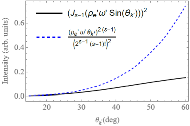
Figure 8: The angular distributions of $|{\bm{A}}^{(f,s)}_{(\text{g})}({\bf k}^{\prime},\omega^{\prime})|^{2}$ in the quasi-classical regime with no SOI, defined by $(J_{s-1}(\rho^{\prime}_{e}\omega^{\prime}\sin\theta_{k^{\prime}}))^{2}$ according to Eq.(127) or by its first expansion term (223). The latter dependence also takes place for undulator radiation at $\varepsilon\gg m_{e}$. Parameters: $\omega=5\,\text{eV},\,\varepsilon/m_{e}=100$ ($m_{e}/\varepsilon\approx 0.57$ deg), $\varepsilon^{\prime}=0.9999\,\varepsilon,\theta^{\prime}\approx 10^{-5}\,\text{rad},\eta=0.5,s=3$.

Thus, not only the emitted energy distributions $|{\bm{E}}^{(f,s)}_{(\text{g})}|^{2}$ are nearly the same for Compton scattering and for emission in a helical undulator in the quasi-classical regime [98], but the phases of the fields do also coincide in this approximation. Importantly, however, the phase $e^{i(s-1)\phi_{k^{\prime}}}$ itself does not guarantee that the field carries angular momentum because the overall factor with the delta-function also plays a role. For instance, if the latter factor contains $\delta(\phi_{k}^{\prime}-(\phi^{\prime}\pm\pi))$ within the conventional plane–wave approach, the TAM $z$-projection is vanishing, regardless of the phase. It is only the generalized-measurement scheme with a finite error that provides vorticity of the final photons because the latter turn out to be cylindrical rather than plane waves.

Appendix D Appendix D: Undulator radiation by a single electron in classical electrodynamics

In classical electrodynamics within the paraxial approximation, the inhomogeneous wave equation for the slowly-varying amplitude of the electric field in the frequency domain $\bm{\widetilde{E}}_{\bot}$ can be written as follows (the Gaussian units with $c=1$ are used):

$$\mathcal{D}\left[\bm{\widetilde{E}}_{\bot}(z,\bm{r}_{\bot},\omega)\right]=\bm{g}_{\bot}(z,\bm{r}_{\bot},\omega)\leavevmode\nobreak\ ,$$ (235)

where the differential operator $\mathcal{D}$ is defined by

$$\mathcal{D}\equiv\left({\nabla_{\bot}}^{2}+{2i\omega}{\partial\over{\partial z}}\right),$$ (236)

${\nabla_{\bot}}^{2}$ being the Laplacian operator over transverse Cartesian coordinates. The source-term vector can be written in terms of the Fourier transform of the transverse current density, $\bm{\bar{j}}_{\bot}(z,\bm{r}_{\bot},\omega)$, and of the charge density, $\bar{\rho}(z,\bm{r}_{\bot},\omega)$ (both being macroscopic quantities treated as given), as

$$\bm{g}_{\bot}=-{4\pi}\exp\left[-i\omega z\right]\left(i\omega\,\bm{\bar{j}}_{\bot}-\bm{\nabla}_{\bot}\bar{\rho}\right).$$ (237)

For a helical undulator, we set a constrained electron motion

$$\bm{r}_{o\bot}(z)=r_{ox}\bm{e}_{x}+r_{oy}\bm{e}_{y}$$ (238)

with

$$r_{ox}(z)=\frac{K}{\gamma_{o}k_{w}}\cos(k_{w}z),\ r_{oy}(z)=\frac{K}{\gamma_{o}k_{w}}\sin(k_{w}z)\leavevmode\nobreak\ .$$ (239)

with the constant longitudinal speed along the $z$ axis. Here

$$k_{w}=\frac{2\pi}{\lambda_{w}},\ K=\frac{{\displaystyle eH_{w}}}{{\displaystyle k_{w}m_{e}}},$$ (240)

$\lambda_{w}$ is an undulator period, and $H_{w}$ is the maximal modulus of the undulator magnetic field on-axis. The classical parameter $K$ is analogous to $\eta$ from Eq.(105).

Solution of the wave equation is found to be:

$$\displaystyle\bm{\widetilde{E}}_{\bot}(z,\bm{r}_{\bot},\omega)=\int_{-\infty}^{z}dz^{\prime}\frac{1}{z-z^{\prime}}\int d\bm{r^{\prime}}_{\bot}\exp\left\{i\omega\left[\frac{\mid\bm{r}_{\bot}-\bm{r^{\prime}}_{\bot}\mid^{2}}{2(z-z^{\prime})}\right]+i\left[\int_{0}^{z^{\prime}}d\bar{z}\frac{\omega}{2{\gamma}_{z}^{2}(\bar{z})}\right]\right\}$$ (241)

$$\displaystyle\times\left[\left(i\omega\bm{v}_{o\bot}(z^{\prime})-\bm{\nabla}^{\prime}_{\bot}\right)\tilde{\rho}(z^{\prime},\bm{r^{\prime}}_{\bot}-\bm{r}_{o\bot}(z^{\prime}),\omega)\right]\leavevmode\nobreak\ ,$$ (242)

(243)

Here $\gamma_{z}(z)=1/\sqrt{1-v_{oz}(z)^{2}}$, and $\bm{\nabla}^{\prime}_{\bot}$ represents the gradient operator with respect to the source point, while $(z,\bm{r}_{\bot})$ indicates the observation point. The further calculations are very similar to those for a planar undulator presented in detail in Ref.[103].

Integration by parts of the gradient term, and introduction of a new integration variable $\bm{l}=\bm{r^{\prime}}_{\bot}-\bm{r}_{o\bot}(z^{\prime})$ gives the following expression in the far-zone limit for relativistic energies, $\gamma\gg 1$, and for the small emission angles $\theta_{x}=x/z\ll 1,\theta_{y}=y/z\ll 1$:

$$\bm{\widetilde{E}}_{\bot}(z,\bm{r}_{\bot},\omega) = -\frac{i\omega}{z}\int d\bm{l}\int_{-\infty}^{\infty}dz^{\prime}\tilde{\rho}(z^{\prime},\bm{l},\omega){\exp{\left[i\Phi_{T}(z^{\prime},\bm{l},\omega)\right]}}$$ (245)

$$\times\left[\left(\frac{K}{\gamma}\sin\left(k_{w}z^{\prime}\right)+\theta_{x}\right)\bm{e}_{x}+\left(-\frac{K}{\gamma}\cos\left(k_{w}z^{\prime}\right)+\theta_{y}\right)\bm{e}_{y}\right]$$

where

$$\displaystyle\Phi_{T}={\omega}\Big{\{}\frac{z^{\prime}}{2\gamma^{2}}\Big{[}1+K^{2}+\gamma^{2}\left(\theta_{x}^{2}+\theta_{y}^{2}\right)\Big{]}-$$ (246)

$$\displaystyle-\frac{K\theta_{x}}{\gamma k_{w}}\cos{(k_{w}z^{\prime})}-\frac{K\theta_{y}}{\gamma k_{w}}\sin{(k_{w}z^{\prime})}\Big{\}}+\Phi_{0}$$ (247)

with $\Phi_{0}=\omega\left[-(\theta_{x}l_{x}+\theta_{y}l_{y})+\frac{z}{2}(\theta_{x}^{2}+\theta_{y}^{2})\right]$. Further use of the resonant approximation leads to

$$\displaystyle\bm{\widetilde{E}}_{\bot s}=\frac{K}{2\gamma}\frac{\omega_{s0}}{z}\int_{-\infty}^{\infty}dl_{x}\int_{-\infty}^{\infty}dl_{y}\int_{-\infty}^{\infty}dz^{\prime}\tilde{\rho}(z^{\prime},\bm{l},\omega)\exp[i\Phi_{0}]\exp\left\{is\frac{\Delta\omega_{s}}{\omega_{s}}k_{w}z^{\prime}\right\}$$ (248)

$$\displaystyle\times\frac{1}{(s-1)!}\left(s\frac{K\gamma}{1+K^{2}}\right)^{s-1}\left(\theta_{y}-i\theta_{x}\right)^{s-1}(\bm{e}_{x}+i\bm{e}_{y}).$$ (249)

where $s$ is the harmonic number (cf. with Sec.5), $\omega=\omega_{s}+\Delta\omega_{s}$. A model for the single-electron emission is obtained by setting

$$\tilde{\rho}({z},\bm{l},\omega)=g_{0}\left(\bm{l}\right)\bar{f}(\omega),$$ (250)

for $z$ in the range $(-L_{w}/2,L_{w}/2)$ and zero otherwise, $L_{w}$ is the undulator length, and $g_{0}=-e\delta{(\bm{l})}$ and $f(t)=\delta(t-t_{e})\longrightarrow\bar{f}(\omega)=\exp(i\omega t_{e})$. The direct substitution explicitly gives

$$\displaystyle\bm{\widetilde{E}}_{\bot s}=-e\frac{K}{2\gamma}\frac{\omega}{z}\exp\left[i\frac{\omega_{s0}z}{2}(\theta_{x}^{2}+\theta_{y}^{2})\right]L_{w}\,\mathrm{sinc}\left[C_{s}L_{w}/z+(\theta_{x}^{2}+\theta_{y}^{2})\omega_{s0}L_{w}/(4)\right]$$ (251)

$$\displaystyle\frac{1}{(s-1)!}\left(s\frac{K\gamma}{1+K^{2}}\right)^{s-1}\left(\theta_{y}-i\theta_{x}\right)^{s-1}(\bm{e}_{x}+i\bm{e}_{y}).$$ (252)

where we have ignored the unimportant phase $\omega t_{e}$. $C_{s}$ is the so-called detuning parameter,

$$\displaystyle C_{s}=\frac{{\displaystyle\omega}}{{\displaystyle 2\bar{\gamma}_{z}^{2}}}-sk_{w}=s\,\frac{{\displaystyle\omega-\omega_{s0}}}{{\displaystyle\omega_{s0}}}\,k_{w},$$ (253)

$$\displaystyle\omega_{s0}=2s\,k_{w}\bar{\gamma}_{z}^{2},\ \bar{\gamma}_{z}^{2}=\frac{{\displaystyle\gamma^{2}}}{{\displaystyle 1+K^{2}}}.$$ (254)

Finally, we note that $\bm{e}_{x}+i\bm{e}_{y}=-\sqrt{2}\,\bm{\chi}_{+1}$ with $\bm{\chi}_{+1}$ from Eq.(202). Going to cylindrical coordinates $\{\theta_{x},\theta_{y}\}=\theta\{\cos\phi,\sin\phi\}$ and an infinitely long undulator, $L_{w}\to\infty$, we obtain in Eq.(252) the same angular dependence and the same phase as for the non-linear Compton (or rather Thomson) scattering in the quasi-classical regime with the circularly polarized laser wave; see Eq.(233) in Sec.C where $\theta_{k^{\prime}},\phi_{k^{\prime}}$ are analogous to $\theta,\phi$, respectively.

References

- [1] L. Allen, M. W. Beijersbergen, R. J. C. Spreeuw, and J. P. Woerdman, Orbital angular momentum of light and the transformation of Laguerre-Gaussian laser modes, Phys. Rev. A 45, 8185 (1992).
- [2] J. P. Torres, L. Torner, Twisted Photons: Applications of Light With Orbital Angular Momentum. Wiley-Vch Verlag, John Wiley and Sons, Weinheim (2011).
- [3] D. L. Andrews, M. Babiker, The Angular Momentum of Light, Cambridge University Press, Cambridge (2012).
- [4] B. A. Knyazev, V. G. Serbo, Beams of photons with nonzero projections of orbital angular momenta: New results, Phys. Usp. 61, 449 (2018).
- [5] F. Tamburini, Bo Thidé, G. Molina-Terriza, G. Anzolin, Twisting of light around rotating black holes, Nat. Phys. 7, 195 (2011).
- [6] D. Budker, J. R. Crespo López-Urrutia, A. Derevianko, V. V. Flambaum, M. W. Krasny, A. Petrenko, S. Pustelny, A. Surzhykov, V. A. Yerokhin, and M. Zolotorev, Atomic physics studies at the Gamma Factory at CERN, Ann. Phys. (Berlin) 532, 2000204 (2020).
- [7] Y. Taira, Y. Kohmura, Measuring the topological charge of an x-ray vortex using a triangular aperture, J. Opt. 21, 045604 (2019).
- [8] I. Ivanov, Double-Twisted Spectroscopy with Delocalized Atoms, Ann. Phys. (Berlin) 2021, 2100128 (2021).
- [9] I. P. Ivanov, B. Liu, P. Zhang, Observability of the superkick effect within a quantum-field-theoretical approach, Phys. Rev. A, 105, 013522 (2022).
- [10] A. Mair, A. Vaziri, G. Weihs, A. Zeilinger, Entanglement of the orbital angular momentum states of photons, Nature 412, 313 (2001).
- [11] D. Bhatti, J. von Zanthier, G. S. Agarwal, Entanglement of polarization and orbital angular momentum, Phys. Rev. A 91, 062303 (2015).
- [12] R. Fickler, G. Campbelld, B. Buchlerd, P. K. Lamd, A. Zeilinger, Quantum entanglement of angular momentum states with quantum numbers up to 10,010, Proc. Nat. Acad. Sci. USA 113, 13642 (2016).
- [13] S. Sasaki, I. McNulty, R. Dejus, Undulator radiation carrying spin and orbital angular momentum, Nuclear Instruments and Methods in Physics Research A 582, 43 (2007).
- [14] S. Sasaki, I. McNulty, Proposal for Generating Brilliant X-Ray Beams Carrying Orbital Angular Momentum, Phys. Rev. Lett. 100, 124801 (2008).
- [15] A. Afanasev, A. Mikhailichenko, On Generation of Photons Carrying Orbital Angular Momentum in the Helical Undulator, arXiv:1109.1603 (2011).
- [16] J. Bahrdt, K. Holldack, P. Kuske, R. Müller, M. Scheer, and P. Schmid, Phys. Rev. Lett. 111, 034801 (2013).
- [17] T. Kaneyasu, Y. Hikosaka, M. Fujimoto, H. Iwayama, M. Hosaka, E. Shigemasac, M. Katoh, Observation of an optical vortex beam from a helical undulator in the XUV region, J. Synchrotron Rad. 24, 934 (2019).
- [18] O. V. Bogdanov, P. O. Kazinski, G. Yu. Lazarenko, Probability of radiation of twisted photons by classical currents, Phys. Rev. A 97, 033837 (2018).
- [19] O. V. Bogdanov, P. O. Kazinski, G. Yu. Lazarenko, Semiclassical probability of radiation of twisted photons in the ultrarelativistic limit, Phys. Rev. D 99, 116016 (2019).
- [20] U. D. Jentschura, V. G. Serbo, Generation of High-Energy Photons with Large Orbital Angular Momentum by Compton Backscattering, Phys. Rev. Lett. 106, 013001 (2011).
- [21] U. D. Jentschura, V. G. Serbo, Compton upconversion of twisted photons: backscattering of particles with non-planar wave functions, Eur. Phys. J. C 71, 1571 (2011).
- [22] Y. Taira, T. Hayakawa, M. Katoh, Gamma-ray vortices from nonlinear inverse Thomson scattering of circularly polarized light, Scientific Reports 7, 5018 (2017).
- [23] M. Katoh, M. Fujimoto, N. S. Mirian, T. Konomi, Y. Taira, T. Kaneyasu, M. Hosaka, N. Yamamoto, A. Mochihashi, Y. Takashima, K. Kuroda, A. Miyamoto, K. Miyamoto, S. Sasaki, Helical Phase Structure of Radiation from an Electron in Circular Motion, Scientific Reports 7, 6130 (2017).
- [24] M. Katoh, M. Fujimoto, H. Kawaguchi, K. Tsuchiya, K. Ohmi, T. Kaneyasu, Y. Taira, M. Hosaka, A. Mochihashi, and Y. Takashima, Angular Momentum of Twisted Radiation from an Electron in Spiral Motion, Phys. Rev. Lett. 118, 094801 (2017).
- [25] V. Epp, U. Guselnikova, Angular momentum of radiation from a charge in circular and spiral motion, Phys. Lett. A 383, 2668 (2019).
- [26] V. Epp, U. Guselnikova, I. Kamenskaya, Angular momentum transferred by the field of a moving point charge, Phys. Rev. A 105, 023511 (2022).
- [27] O. V. Bogdanov, P. O. Kazinski, G. Yu. Lazarenko, Proposal for experimental observation of the twisted photons in transition and Vavilov-Cherenkov radiations, JINST 15, C04052 (2020).
- [28] O. V. Bogdanov, P. O. Kazinski, P. S. Korolev, G. Yu. Lazarenko, Radiation of twisted photons from charged particles moving in cholesterics, Journal of Molecular Liquids 326, 115278 (2021).
- [29] S. V. Abdrashitov, O. V. Bogdanov, P. O. Kazinski, and T. A. Tukhfatullin, Orbital angular momentum of channeling radiation from relativistic electrons in thin Si crystal, Phys. Lett. A 382, 3141 (2018).
- [30] V. Epp, J. Janz, and M. Zotova, Angular momentum of radiation at axial channeling, Nucl. Instrum. Methods Phys. Res. B 436, 78 (2018).
- [31] D. V. Karlovets, V. G. Serbo, A. Surzhykov, Wave function of a photon produced in the resonant scattering of twisted light by relativistic ions, Phys. Rev. A 104, 023101 (2021)
- [32] K. Yu. Bliokh, M. R. Dennis, and F. Nori, Relativistic Electron Vortex Beams: Angular Momentum and Spin-Orbit Interaction, Phys. Rev. Lett. 107, 174802 (2011).
- [33] K.Y. Bliokh, I.P. Ivanov, G. Guzzinati, L. Clark, R. Van Boxem, A. Béchéd, R. Juchtmans, M.A. Alonso, P. Schattschneider, F. Nori, J. Verbeeck, Theory and applications of free-electron vortex states, Phys. Rep. 690, 1 (2017).
- [34] M. Uchida and A. Tonomura, Generation of electron beams carrying orbital angular momentum, Nature 464, 737 (2010).
- [35] J. Verbeeck, H. Tian, P. Schlattschneider, Production and application of electron vortex beams, Nature 467, 301 (2010).
- [36] B. J. McMorran A. Agrawal, I. M. Anderson, et al., Electron vortex beams with high quanta of orbital angular momentum, Science 331, 192 (2011).
- [37] T. ihek, M. Hork, T. Schachinger, et al., Beam shaping and probe characterization in the scanning electron microscope, Ultramicroscopy 225, 113268 (2021).
- [38] E. Mafakheri, A. H. Tavabi, P.-H. Lu et al., Realization of electron vortices with large orbital angular momentum using miniature holograms fabricated by electron beam lithography, Appl. Phys. Lett. 110, 093113 (2017).
- [39] A.H. Tavabi, P. Rosi, A. Roncaglia, E. Rotunno, M. Beleggia, P.H. Lu, L. Belsito, G. Pozzi, S. Frabboni, P. Tiemeijer, et al., Generation of electron vortex beams with over 1000 orbital angular momentum quanta using a tuneable electrostatic spiral phase plate, Appl. Phys. Lett. 121, 073506 (2022).
- [40] R. Juchtmans, A. Bch, A. Abakumov, M. Batuk, and J. Verbeeck, Using electron vortex beams to determine chirality of crystals in transmission electron microscopy, Phys. Rev. B 91, 094112 (2015).
- [41] S. M. Lloyd, M. Babiker, G. Thirunavukkarasu, and J. Yuan, Electron vortices: Beams with orbital angular momentum, Rev. Mod. Phys. 89, 035004 (2017).
- [42] I. P. Ivanov, Colliding particles carrying non-zero orbital angular momentum, Phys. Rev. D 83, 093001 (2011).
- [43] I. P. Ivanov, V. G. Serbo, Scattering of twisted particles: Extension to wave packets and orbital helicity, Phys. Rev. A 84, 033804 (2011).
- [44] D. V. Karlovets, Electron with orbital angular momentum in a strong laser wave, Phys. Rev. A 86, 062102 (2012).
- [45] I.P. Ivanov, Creation of two vortex-entangled beams in a vortex-beam collision with a plane wave, Phys. Rev. A 85, 033813 (2012).
- [46] I. P. Ivanov, Measuring the phase of the scattering amplitude with vortex beams, Phys. Rev. D 85, 076001 (2012).
- [47] D. Seipt, A. Surzhykov, and S. Fritzsche, Structured x-ray beams from twisted electrons by inverse Compton scattering of laser light, Phys. Rev. A 90, 012118 (2014).
- [48] V. G. Serbo, I. Ivanov, S. Fritzsche, D. Seipt, A. Surzhykov, Scattering of twisted relativistic electrons by atoms, Phys. Rev. A 92 012705, (2015).
- [49] I. Kaminer, M. Mutzafi, A. Levy, G. Harari, H. H. Sheinfux, S. Skirlo, J. Nemirovsky, J. D. Joannopoulos, M. Segev, and M. Soljai, Quantum erenkov Radiation: Spectral Cutoffs and the Role of Spin and Orbital Angular Momentum, Phys. Rev. X 6, 011006 (2016).
- [50] I. P. Ivanov, V. G. Serbo, and V. A. Zaytsev, Quantum calculation of the Vavilov-Cherenkov radiation by twisted electrons, Phys. Rev. A 93, 053825 (2016).
- [51] I. P. Ivanov, D. Seipt, A. Surzhykov, S. Fritzsche, Elastic scattering of vortex electrons provides direct access to the Coulomb phase, Phys. Rev. D 94, 076001 (2016).
- [52] D. V. Karlovets, Scattering of wave packets with phases, J. High Energy Phys. 03, 049 (2017).
- [53] J. A. Sherwin, Compton scattering of Bessel light with large recoil parameter, Phys. Rev. A 96, 062120 (2017).
- [54] J. A. Sherwin, Two-photon annihilation of twisted positrons, Phys. Rev. A 98, 042108 (2018).
- [55] D. V. Karlovets, V. G. Serbo, Effects of the transverse coherence length in relativistic collisions, Phys. Rev. D 101, 076009 (2020).
- [56] I. P. Ivanov, N. Korchagin, A. Pimikov, and P. Zhang, Doing spin physics with unpolarized particles, Phys. Rev. Lett. 124, 192001 (2020).
- [57] I. P. Ivanov, N. Korchagin, A. Pimikov, and P. Zhang, Twisted particle collisions: a new tool for spin physics, Phys. Rev. D 101, 096010 (2020).
- [58] I. P. Ivanov, N. Korchagin, A. Pimikov, and P. Zhang, Kinematic surprises in twisted-particle collisions, Phys. Rev. D 101, 016007 (2020).
- [59] I. Madan, G. M. Vanacore, S. Gargiulo, T. LaGrange, and F. Carbone, The quantum future of microscopy: Wave function engineering of electrons, ions, and nuclei, Appl. Phys. Lett. 116, 230502 (2020).
- [60] P. Zhao, I.P. Ivanov, P. Zhang, Decay of the vortex muon, Phys. Rev. D 104, 036003 (2021).
- [61] A. V. Maiorova, A. V. Peshkov, A. A. Surzhykov, Radiative recombination of twisted electrons with hydrogenlike heavy ions: Linear polarization of emitted photons, Phys. Rev. A 104, 022821 (2021).
- [62] A. A. Peshkov, Y. M. Bidasyuk, R. Lange, N. Huntemann, E. Peik, and A. Surzhykov, Interaction of twisted light with a trapped atom: Interplay between electronic and motional degrees of freedom, Phys. Rev. A 107, 023106 (2023).
- [63] L. Zou, P. Zhang, A. J. Silenko, Production of twisted particles in heavy-ion collisions, J. Phys. G: Nucl. Part. Phys. 50, 015003 (2023).
- [64] I. P. Ivanov, Promises and challenges of high-energy vortex states collisions, Progress in Particle and Nuclear Physics 127, 103987 (2022); https://doi.org/10.1016/j.ppnp.2022.103987.
- [65] K. Floettmann, and D. Karlovets, Quantum mechanical formulation of the Busch theorem, Phys. Rev. A 102, 043517 (2020).
- [66] D. Karlovets, Vortex particles in axially symmetric fields and applications of the quantum Busch theorem, New J. Phys. 23, 033048 (2021).
- [67] A. Burov, S. Nagaitsev, Y. Derbenev, Circular modes, beam adapters, and their applications in beam optics, Phys. Rev. E 66, 016503 (2002).
- [68] K.-J. Kim, Round-to-flat transformation of angular-momentum-dominated beams, Phys. Rev. ST Accel. Beams 6, 104002 (2003).
- [69] Y.-E Sun, P. Piot, K.-J. Kim, N. Barov, S. Lidia, J. Santucci, R. Tikhoplav, J. Wennerberg, Generation of angular-momentum-dominated electron beams from a photoinjector, Phys. Rev. ST Accel. Beams 7, 123501 (2004).
- [70] L. Groening, C. Xiao, M. Chung, Particle beam eigenemittances, phase integral, vorticity, and rotations, Phys. Rev. Accel. Beams 24, 054201 (2021).
- [71] C. Jia, D. Ma, A. F. Schäffer, J. Berakdar, Twisted magnon beams carrying orbital angular momentum, Nature Comm. 10, 2077 (2019).
- [72] A. V. Afanasev, D. V. Karlovets, V. G. Serbo, Elastic scattering of twisted neutrons by nuclei, Phys. Rev. C 103, 054612 (2021).
- [73] A. Luski, Y. Segev, R. David, O. Bitton, H. Nadler, A. R. Barnea, A. Gorlach, O. Cheshnovsky, I. Kaminer, E. Narevicius, Vortex beams of atoms and molecules, Science 373, 1105 (2021).
- [74] A. Bch, R. van Boxem, G. van Tendeloo, J. Verbeeck, Magnetic monopole field exposed by electrons, Nat. Phys. 10, 26 (2014).
- [75] Ch.W. Clark, R. Barankov, M.G. Huber, M, Arif, D.G. Cory, and D.A. Pushin, Controlling neutron orbital angular momentum, Nature 525, 504 (2015).
- [76] C. Greenshields, R.L. Stamps, S. Franke-Arnold, Vacuum Faraday effect for electrons, Phys. Rev. Lett. 113 (2014) 240404.
- [77] C.R. Greenshields, R.L. Stamps, S. Franke-Arnold, S.M. Barnett, Is the angular momentum of an electron conserved in a uniform magnetic field? Phys. Rev. Lett. 113 (2014) 240404.
- [78] C. Greenshields, S. Franke-Arnold, R.L. Stamps, Parallel axis theorem for free-space electron wavefunctions, New J. Phys. 17 (2015) 093015.
- [79] A. A. Sokolov, I. M. Ternov, Relativistic electron, Nauka, Moscow, (1974) [in Russian] [Radiation from Relativistic Electrons, Edited by C. W. Kilmister, American Institute of Physics Translation Series, New York, (1986)].
- [80] D. V. Karlovets, S. S. Baturin, G. Geloni, G. K. Sizykh, and V. G. Serbo, Generation of vortex particles via generalized measurements, Eur. Phys. J. C 82, 1008 (2022).
- [81] D. Budker, J. C. Berengut, V. V. Flambaum, M. Gorchtein, J. Jin, F. Karbstein, M. W. Krasny, Y. A. Litvinov, A. Pálffy, V. Pascalutsa, A. Petrenko, A. Surzhykov, P. G. Thirolf, M. Vanderhaeghen, H. A. Weidenmüller, V. Zelevinsky, Expanding Nuclear Physics Horizons with the Gamma Factory, Annalen der Physik 534, 2100284 (2022).
- [82] V. B. Berestetskii, E. M. Lifshitz and L. P. Pitaevskii, Quantum Electrodynamics, Oxford: Pergamon, 1982.
- [83] M. E. Peskin, D. V. Schroeder, An introduction to quantum field theory (Westview Press, 1995).
- [84] S.M. Barnett, Quantum information (New York, Oxford University Press, 2009).
- [85] M. A. Al Khafaji, C. M. Cisowski, H. Jimbrown, S. Croke, S. Pádua, and S. Franke-Arnold, Single-shot characterization of vector beams by generalized measurements, Optics Express 30, 22396 (2022).
- [86] P. Carruthers, M. M. Nieto, Phase and angle variables in quantum mechanics, Rev. Mod. Phys. 40, 411 (1968).
- [87] S. Franke-Arnold, S.M. Barnett, E. Yao, J. Leach, J. Courtial, and M. Padgett, Uncertainty principle for angular position and angular momentum, New J. Phys. 6, 103 (2004).
- [88] M. O. Scully, M. S. Zubairy, Quantum optics (Cambridge University Press, 1997).
- [89] Y. Aharonov, D. Z. Albert, L. Vaidman, How the result of a measurement of a component of the spin of a spin- particle can turn out to be 100, Phys. Rev. Lett. 60, 1351 (1988).
- [90] Y. Aharonov and D. Rohrlich, Quantum Paradoxes: Quantum Theory for the Perplexed, WILEY-VCH Verlag GmbH & Co. KGaA, Weinheim, 2005.
- [91] B. Tamir, E. Cohen, Introduction to Weak Measurements and Weak Values, Quanta 2, 7 (2013).
- [92] Y. Aharonov, E. Cohen, A. C. Elitzur, Foundations and applications of weak quantum measurements, Phys. Rev. A 89, 052105 (2014).
- [93] V. G. Bagrov, D. M. Gitman, and A. S. Pereira, Coherent and semiclassical states of a free particle, Phys.-Usp. 57, 891 (2014).
- [94] V.I. Ritus, J. Russ. Laser Res. 6, 497 (1985).
- [95] A. Di Piazza, C. Müller, K. Z. Hatsagortsyan, and C. H. Keitel, Extremely high-intensity laser interactions with fundamental quantum systems, Rev. Mod. Phys. 84, 1177 (2012).
- [96] A. Fedotov, A. Ilderton, F. Karbstein, B. King, D. Seipt, H. Taya, G. Torgrimsson, Advances in QED with intense background fields, Phys. Rep. 1010, 1 (2023).
- [97] J. Gea-Banacloche, Quantum theory of the free-electron laser: Large gain, saturation, and photon statistics, Phys. Rev. A 31, 1607 (1985).
- [98] T. Heinzl, A. Ilderton, and B. King, Classical and quantum particle dynamics in univariate background fields, Phys. Rev. D 94, 065039 (2016).
- [99] A. Halavanau, D. Seipt, I. Lobach, T. Raubenheimer, S. Nagaitsev, Z. Huang, C. Pellegrini, Undulator radiation generated by a single electron, Proc. 10th Int. Particle Accelerator Conf. (IPAC’19), Melbourne, Australia, May 2019, pp. 1867-1870; doi:10.18429/JACoW-IPAC2019-TUPRB089.
- [100] L.D. Landau, E.M. Lifshitz, The Classical Theory of Fields (Oxford, Pergamon, 1975).
- [101] D. Yu. Ivanov, G. L. Kotkin, V. G. Serbo, Complete description of polarization effects in emission of a photon by an electron in the field of a strong laser wave, Eur. Phys. J. C 36, 127 (2004).
- [102] D. A. Varshalovich, A. N. Moskalev, and V. K. Khersonskii, Quantum Theory of Angular Momentum (World Scientific, Singapore, 1988).
- [103] G. Geloni, V. Kocharyan, and E. Saldin, Theoretical computation of the polarization characteristics of an X-ray Free-Electron Laser with planar undulator, Optics Comm. 356, 435 (2015).
- [104] D. Karlovets, A. Di Piazza, Emission of twisted photons by a scalar charge in a strong magnetic field, arXiv:2303.01946 (2022).
- [105] S. Karabekyan, S. Abeghyan, M. Bagha-Shanjani, S. Casalbuoni, W. Freund, et al., The status of the SASE3 variable polarization project at the European XFEL, Proc. 13th International Particle Accelerator Conference – IPAC’22, Bangkok, Thailand, Jun. 2022, pp. 1029–1032.