Certifying the Intersection of Reach Sets of Integrator Agents
with Set-valued Input Uncertainties

Shadi Haddad and Abhishek Halder Shadi Haddad and Abhishek Halder are with the Department of Applied Mathematics, University of California, Santa Cruz, CA 95064, USA, {shhaddad,halder}@ucsc.edu.
Abstract

We consider the problem of verifying safety for a pair of identical integrator agents in continuous time with compact set-valued input uncertainties. We encode this verification problem as that of certifying or falsifying the intersection of their reach sets. We transcribe the same into a variational problem, namely that of minimizing the support function of the difference of the two reach sets over the unit sphere. We illustrate the computational tractability of the proposed formulation by developing two cases in detail, viz. when the inputs have time-varying norm-bounded and generic hyperrectangular uncertainties. We show that the latter case allows distributed certification via second order cone programming.

I Introduction

We consider a pair of integrator agents labeled as A and B, each with $n$ states, $m$ inputs and relative degree $\bm{r}=(r_{1},\ldots,r_{m})^{\top}\in\mathbb{N}^{m}$ where $r_{1}+\ldots+r_{m}=n$. For example, when $n=5$, $m=2$, and $\bm{r}=(3,2)^{\top}$, then the individual integrator agent dynamics in continuous time is of the form

$\displaystyle\dot{\bm{x}}^{i}=\left(\begin{array}[]{@{}ccc|cc@{}}0&1&0&0&0\\ 0&0&1&0&0\\ 0&0&0&0&0\\ \hline\cr 0&0&0&0&1\\ 0&0&0&0&0\\ \end{array}\right)\bm{x}^{i}+\left(\begin{array}[]{@{}c|c@{}}0&0\\ 0&0\\ 1&0\\ \hline\cr 0&0\\ 0&1\end{array}\right)\bm{u}^{i},$ (11)

wherein for $i\in\{\texttt{A},\texttt{B}\}$, the vectors $\bm{x}^{i},\bm{u}^{i}$ respectively denote the state and input of the agents A and B.

In general, for $i\in\{\texttt{A},\texttt{B}\}$, the integrator agent dynamics takes the form

$\displaystyle\dot{\bm{x}}^{i}\!=\!\underbrace{\mathrm{bldiag}\left(\bm{A}_{1},\ldots,\bm{A}_{m}\right)}_{=:\bm{A}}\!\bm{x}^{i}\!+\!\underbrace{\mathrm{bldiag}\left(\bm{b}_{1},\ldots,\bm{b}_{m}\right)}_{=:\bm{B}}\!\bm{u}^{i},$ (12)

where $\mathrm{bldiag}\left(\cdot\right)$ denotes block diagonal matrix whose arguments constitute its diagonal blocks, and

$\displaystyle\bm{A}_{j}:=\left(\mathbf{0}_{r_{j}\times 1}\left|\bm{e}_{1}^{r_{j}}\right|\bm{e}_{2}^{r_{j}}|\ldots|\bm{e}_{r_{j}-1}^{r_{j}}\right),\quad\bm{b}_{j}:=\bm{e}_{r_{j}}^{r_{j}},$ (13)

for $j\in[m]:=\{1,2,\ldots,m\}$. In (13), the notation $\mathbf{0}_{r_{j}\times 1}$ stands for the vector of zeros of size $r_{j}\times 1$. For $k\leq\ell$, we use $\bm{e}_{k}^{\ell}$ to denote the $k$th standard basis column vector in $\mathbb{R}^{\ell}$.

In this work, we consider the problem of checking whether the agents A and B, starting from respective initial conditions $\bm{x}_{0}^{\texttt{A}},\bm{x}_{0}^{\texttt{B}}\in\mathbb{R}^{n}$, and respective input uncertainties modeled as compact111This means that the set-valued trajectories in (14) are continuous w.r.t. s๐‘ s, and the sets are compact for all 0โ‰คsโ‰คt0๐‘ ๐‘ก0\leq s\leq t. input set-valued trajectories

๐’ฐAโ€‹(s),๐’ฐBโ€‹(s)โŠ‚โ„m,0โ‰คsโ‰คt,formulae-sequencesuperscript๐’ฐA๐‘ superscript๐’ฐB๐‘ superscriptโ„๐‘š0๐‘ ๐‘ก\displaystyle\mathcal{U}^{\texttt{A}}(s),\,\mathcal{U}^{\texttt{B}}(s)\subset\mathbb{R}^{m},\quad 0\leq s\leq t, (14)

may result in intersecting reach sets $\mathcal{X}_{t}^{\texttt{A}},\mathcal{X}_{t}^{\texttt{B}}\subset\mathbb{R}^{n}$ at a given time $t$. Formally, the (forward) reach sets are given by

๐’ณti:=โ‹ƒmeasurableโ€‹๐’–iโ€‹(โ‹…)โˆˆ๐’ฐiโ€‹(โ‹…){๐’™i(t)โˆˆโ„nโˆฃ(12),๐’™i(t=0)=๐’™0i,\displaystyle\!\mathcal{X}_{t}^{i}:=\!\!\!\bigcup_{\text{measurable}\;\bm{u}^{i}(\cdot)\in\mathcal{U}^{i}(\cdot)}\!\{\bm{x}^{i}(t)\in\mathbb{R}^{n}\mid\eqref{IntegratorODE},\;\bm{x}^{i}(t=0)=\bm{x}_{0}^{i},
$\displaystyle\bm{u}^{i}(s)\in\mathcal{U}^{i}(s)\;\text{compact for all}\;0\leq s\leq t\},\;i\in\{\texttt{A},\texttt{B}\},$ (15)

such that $\bm{x}_{0}^{i}=(\bm{x}_{10}^{i},\ldots,\bm{x}_{m0}^{i})^{\top}\subset\mathbb{R}^{n}$. In words, the forward reach set at time $t$ is the set of states that the individual agent may reach subject to its integrator dynamics, given initial condition and compact set-valued input uncertainties. In this paper, we only consider reach sets forward in time, and hereafter refer to the same as reach sets.

It is well-known [1] that the reach sets $\mathcal{X}_{t}^{i}$ in (15) are compact convex provided the input sets (14) are compact. Furthermore, the sets $\mathcal{X}_{t}^{i}$ are invariant under the closure of convexification of the input sets (14); see e.g., [2, Prop. 6.1, Thm. 6.3]. We would like to certify (or falsify) if ๐’ณtAโˆฉ๐’ณtBโ‰ (=)โ€‹โˆ…superscriptsubscript๐’ณ๐‘กAsuperscriptsubscript๐’ณ๐‘กB\mathcal{X}_{t}^{\texttt{A}}\cap\mathcal{X}_{t}^{\texttt{B}}\neq(=)\varnothing at a given time $t$.

Collision detection and avoidance for integrator agents have received attention [3, 4, 5, 6] in the robotics literature. Beyond serving as simple models for agent dynamics, integrators also arise as Brunovsky normal forms of feedback linearizable systems resulting from a diffeomorphic change of state coordinates. On the other hand, detecting intersection of reach sets amounts to verifying safe operation in the sense of checking separability of the agentsโ€™ states or lack thereof subject to set-valued uncertainties. In particular, detecting the intersection of reach sets of static state feedback linearizable systems, can be shown222See Supplementary Material to be equivalent to detecting the same in the normal coordinates. With this motivation, the present work investigates certifying the intersection of reach sets of integrator agents using ideas from convex geometry.

The organization of this paper is as follows. In Sec. II, we provide some background on the support function of a compact convex set in general, and that of the integrator reach set in particular. In Sec. III, we formulate the problem of detecting intersection among the reach sets of two integrator agents, labeled as A and B, as that of solving a nonconvex problem involving their support functions. We next show that when the input uncertainty sets are time-varying norm balls (Sec. IV) or time-varying generic hyperrectangles (Sec. V), then a lossless convexification of the nonconvex formulation solves the intersection detection problem.

II Background on Support Function

The support function $h_{\mathcal{K}}(\cdot)$ of a compact convex set $\mathcal{K}\subset\mathbb{R}^{n}$, is given by

$\displaystyle h_{\mathcal{K}}(\bm{y}):=\underset{\bm{x}\in\mathcal{K}}{\sup}\>\{\langle\bm{y},\bm{x}\rangle\mid\bm{y}\in\mathbb{S}^{n-1}\},$ (16)

where $\langle\cdot,\cdot\rangle$ denotes the standard Euclidean inner product, and $\mathbb{S}^{n-1}$ is the unit sphere embedded in $\mathbb{R}^{n}$. For details on the support function, we refer the readers to [7, Ch. V].

The following result (proof in Appendix -A) will come in handy in the ensuing development.

Proposition 1.

Consider the integrator dynamics with $n$ states, $m$ inputs, and relative degree vector $\bm{r}=(r_{1},\ldots,r_{m})^{\top}\in\mathbb{N}^{m}$. For compact input uncertainty sets ๐’ฐโ€‹(s)โŠ‚โ„m๐’ฐ๐‘ superscriptโ„๐‘š\mathcal{U}(s)\subset\mathbb{R}^{m}, 0โ‰คsโ‰คt0๐‘ ๐‘ก0\leq s\leq t, the support function of the integrator reach set $\mathcal{X}_{t}$ at time $t$ starting from the initial condition $\bm{x}_{0}=\left(\bm{x}_{10},\bm{x}_{20},\ldots,\bm{x}_{m0}\right)^{\top}\in\mathbb{R}^{n}$, is given by

$\displaystyle h_{\mathcal{X}_{t}}\left(\bm{y}\right)$ $\displaystyle=\sum_{j=1}^{m}~{}\langle\bm{y}_{j},\exp\left(t\bm{A}\right)\bm{x}_{j0}\rangle$
+โˆซ0tsup๐’–โ€‹(s)โˆˆ๐’ฐโ€‹(s)โ€‹โˆ‘j=1mโŸจ๐’šj,๐ƒjโ€‹(s)โŸฉโ€‹ujโ€‹(s)โ€‹dโ€‹s,subscriptsuperscript๐‘ก0๐’–๐‘ ๐’ฐ๐‘ supremumsuperscriptsubscript๐‘—1๐‘šsubscript๐’š๐‘—subscript๐ƒ๐‘—๐‘ subscript๐‘ข๐‘—๐‘ d๐‘ \displaystyle\quad+\int^{t}_{0}\underset{\bm{u}(s)\in\mathcal{U}(s)}{\sup}\sum_{j=1}^{m}\langle\bm{y}_{j},\bm{\xi}_{j}(s)\rangle\>u_{j}(s)\>{\rm{d}}{s}, (17)

where the subvector $\bm{x}_{j0}\in\mathbb{R}^{r_{j}}$, $j\in[m]$, and

๐ƒjโ€‹(s):=(srjโˆ’1/(rjโˆ’1)!srjโˆ’2/(rjโˆ’2)!โ‹ฎs1),๐ƒโ€‹(s):=(๐ƒ1โ€‹(s)โ‹ฎ๐ƒmโ€‹(s)).formulae-sequenceassignsubscript๐ƒ๐‘—๐‘ matrixsuperscript๐‘ subscript๐‘Ÿ๐‘—1subscript๐‘Ÿ๐‘—1superscript๐‘ subscript๐‘Ÿ๐‘—2subscript๐‘Ÿ๐‘—2โ‹ฎ๐‘ 1assign๐ƒ๐‘ matrixsubscript๐ƒ1๐‘ โ‹ฎsubscript๐ƒ๐‘š๐‘ \displaystyle\bm{\xi}_{j}(s):=\!\begin{pmatrix}s^{r_{j}-1}/(r_{j}-1)!\\ s^{r_{j}-2}/(r_{j}-2)!\\ \vdots\\ s\\ 1\end{pmatrix},~{}\bm{\xi}(s):=\!\begin{pmatrix}\bm{\xi}_{1}(s)\\ \vdots\\ \bm{\xi}_{m}(s)\end{pmatrix}. (18)

The proof in Appendix -A reveals a relationship between the support function of the reach set $\mathcal{X}_{t}$ with that of the compact input sets ๐’ฐโ€‹(s)๐’ฐ๐‘ \mathcal{U}(s), 0โ‰คsโ‰คt0๐‘ ๐‘ก0\leq s\leq t, given by

h๐’ณtโ€‹(๐’š)=โŸจ๐’š,expโก(tโ€‹๐‘จ)โ€‹๐’™0โŸฉ+โˆซ0th๐’ฐโ€‹(s)โ€‹((expโก(sโ€‹๐‘จ)โ€‹๐‘ฉ)โŠคโ€‹๐’š)โ€‹ds.subscriptโ„Žsubscript๐’ณ๐‘ก๐’š๐’š๐‘ก๐‘จsubscript๐’™0superscriptsubscript0๐‘กsubscriptโ„Ž๐’ฐ๐‘ superscript๐‘ ๐‘จ๐‘ฉtop๐’šdifferential-d๐‘ \displaystyle h_{\mathcal{X}_{t}}(\bm{y})=\langle\bm{y},\exp(t\bm{A})\bm{x}_{0}\rangle\!+\!\!\int_{0}^{t}\!\!\!h_{\mathcal{U}(s)}\!\!\left(\!\left(\exp(s\bm{A})\bm{B}\right)^{\top}\!\!\bm{y}\!\right)\!{\rm{d}}s. (19)

When ๐’ฐโ€‹(s)๐’ฐ๐‘ \mathcal{U}(s) is compact nonconvex, then h๐’ฐโ€‹(s)โ€‹(โ‹…)subscriptโ„Ž๐’ฐ๐‘ โ‹…h_{\mathcal{U}(s)}(\cdot) is the support function of the closure of the convex hull of ๐’ฐโ€‹(s)๐’ฐ๐‘ \mathcal{U}(s).

III Problem Formulation

One way to check if $\mathcal{X}_{t}^{\texttt{A}}\cap\mathcal{X}_{t}^{\texttt{B}}=\varnothing$ or not, is to compute the distance between the reach sets $\mathcal{X}_{t}^{\texttt{A}},\mathcal{X}_{t}^{\texttt{B}}$, given by

$\displaystyle{\rm{dist}}\left(\texttt{A},\texttt{B}\right):=\underset{\stackrel{{\scriptstyle}}{{\bm{x}^{\texttt{A}}\in\mathcal{X}_{t}^{\texttt{A}},\bm{x}^{\texttt{B}}\in\mathcal{X}_{t}^{\texttt{B}}}}}{\min}\;\|\bm{x}^{\texttt{A}}-\bm{x}^{\texttt{B}}\|_{2}^{2}.$ (20)

Clearly, ${\rm{dist}}\left(\texttt{A},\texttt{B}\right)>0$ if and only if $\mathcal{X}_{t}^{\texttt{A}}\cap\mathcal{X}_{t}^{\texttt{B}}=\varnothing$, and $=0$ otherwise. However, computing the distance between the reach sets $\mathcal{X}_{t}^{\texttt{A}},\mathcal{X}_{t}^{\texttt{B}}$ requires analytic handle on the boundary of these reach sets, which can be computationally difficult depending on the geometry of the input sets (14).

To circumvent this difficulty, we take an alternative approach based on the difference set of $\mathcal{X}_{t}^{\texttt{A}}$ and $\mathcal{X}_{t}^{\texttt{B}}$, given by the compact convex set

$\displaystyle\mathcal{X}_{t}^{\texttt{A}}\mathbin{\text{\ooalign{\raise 4.30554pt\hbox{.}\cr$-$\cr}}}\mathcal{X}_{t}^{\texttt{B}}:=\{\bm{x}^{\texttt{A}}-\bm{x}^{\texttt{B}}\mid\bm{x}^{\texttt{A}}\in\mathcal{X}_{t}^{\texttt{A}},\bm{x}^{\texttt{B}}\in\mathcal{X}_{t}^{\texttt{B}}\}.$ (23)

Notice that $\mathcal{X}_{t}^{\texttt{A}}\mathbin{\text{\ooalign{\raise 4.30554pt\hbox{.}\cr$-$\cr}}}\mathcal{X}_{t}^{\texttt{B}}=\mathcal{X}_{t}^{\texttt{A}}\dotplus\left(-\mathcal{X}_{t}^{\texttt{B}}\right)$ where $\dotplus$ denotes the Minkowski sum, and $\mathcal{X}_{t}^{\texttt{A}}\mathbin{\text{\ooalign{\raise 4.30554pt\hbox{.}\cr$-$\cr}}}\mathcal{X}_{t}^{\texttt{B}}$ is not the same as the Minkowski a.k.a. Pontryagin difference [8, p. 139], [9].

Checking the intersection between $\mathcal{X}_{t}^{\texttt{A}}$ and $\mathcal{X}_{t}^{\texttt{B}}$, is then equivalent to verifying if the zero vector $\bm{0}\in\mathbb{R}^{n}$ belongs to the set (23). This can in turn be related [10, 11] to conditions on the support function $h_{\mathcal{X}_{t}^{\texttt{A}}\mathbin{\text{\ooalign{\raise 3.01389pt\hbox{.}\cr$-$\cr}}}\mathcal{X}_{t}^{\texttt{B}}}(\cdot)$, because

$\displaystyle\mathcal{X}_{t}^{\texttt{A}}\cap\mathcal{X}_{t}^{\texttt{B}}\neq\varnothing\>\Leftrightarrow\>\bm{0}\!\in\!\{\mathcal{X}_{t}^{\texttt{A}}\mathbin{\text{\ooalign{\raise 4.30554pt\hbox{.}\cr$-$\cr}}}\mathcal{X}_{t}^{\texttt{B}}\}$ (24c)
$\displaystyle\hskip 61.42993pt\Leftrightarrow\>\forall\;\bm{y}\in\mathbb{S}^{n-1},h_{\mathcal{X}_{t}^{\texttt{A}}\mathbin{\text{\ooalign{\raise 3.01389pt\hbox{.}\cr$-$\cr}}}\mathcal{X}_{t}^{\texttt{B}}}(\bm{y})\geq 0,$ (24f)
$\displaystyle\mathcal{X}_{t}^{\texttt{A}}\cap\mathcal{X}_{t}^{\texttt{B}}=\varnothing\>\Leftrightarrow\>\bm{0}\!\notin\!\{\mathcal{X}_{t}^{\texttt{A}}\mathbin{\text{\ooalign{\raise 4.30554pt\hbox{.}\cr$-$\cr}}}\mathcal{X}_{t}^{\texttt{B}}\}$ (24i)
$\displaystyle\hskip 61.42993pt\Leftrightarrow\>\exists\;\bm{y}\in\mathbb{S}^{n-1}\,\text{such that}\>h_{\mathcal{X}_{t}^{\texttt{A}}\mathbin{\text{\ooalign{\raise 3.01389pt\hbox{.}\cr$-$\cr}}}\mathcal{X}_{t}^{\texttt{B}}}(\bm{y})<0.$ (24l)

Thus motivated, we propose certifying or falsifying the reach set intersection by computing

$\displaystyle\underset{\bm{y}\in\mathbb{S}^{n-1}}{\min}\>h_{\mathcal{X}_{t}^{\texttt{A}}\mathbin{\text{\ooalign{\raise 3.01389pt\hbox{.}\cr$-$\cr}}}\mathcal{X}_{t}^{\texttt{B}}}(\bm{y}).$ (27)

Specifically, (27) โ‰ฅ(<)โ€‹0โ‡”๐’ณtAโˆฉ๐’ณtBโ‰ (=)โ€‹โˆ…โ‡”absent0superscriptsubscript๐’ณ๐‘กAsuperscriptsubscript๐’ณ๐‘กB\geq(<)0\>\Leftrightarrow\>\mathcal{X}_{t}^{\texttt{A}}\cap\mathcal{X}_{t}^{\texttt{B}}\neq(=)\varnothing. In other words, the optimal cost (27) can be used to certify or falsify the reach set intersection.

Remark 1.

In general, which of the two problems (20) and (27) is computationally more tractable, depends on the sets $\mathcal{X}_{t}^{\texttt{A}},\mathcal{X}_{t}^{\texttt{B}}$. For instance, when $\mathcal{X}_{t}^{\texttt{A}},\mathcal{X}_{t}^{\texttt{B}}$ are ellipsoids, simple algorithms are known [12] for solving (20), but solving (27) requires heavier computation [13]. In the ensuing sections, we explain how detecting the intersection between the integrator reach sets $\mathcal{X}_{t}^{\texttt{A}},\mathcal{X}_{t}^{\texttt{B}}$ using (27) turns out to be computationally more benign than (20).

Since support function is distributive over the Minkowski sum, we have

$\displaystyle h_{\mathcal{X}_{t}^{\texttt{A}}\mathbin{\text{\ooalign{\raise 3.01389pt\hbox{.}\cr$-$\cr}}}\mathcal{X}_{t}^{\texttt{B}}}(\bm{y})=h_{\mathcal{X}_{t}^{\texttt{A}}}(\bm{y})+h_{-\mathcal{X}_{t}^{\texttt{B}}}(\bm{y}).$ (30)

From the definition of support function, we also have

$\displaystyle\!\!\!\!h_{-\mathcal{X}_{t}^{\texttt{B}}}(\bm{y})=\!\underset{\bm{x}\in-\mathcal{X}_{t}^{\texttt{B}}}{\sup}\langle\bm{y},\bm{x}\rangle$ $\displaystyle=\underset{\bm{x}\in\mathcal{X}_{t}^{\texttt{B}}}{\sup}\langle\bm{y},-\bm{x}\rangle$
$\displaystyle=\underset{\bm{x}\in\mathcal{X}_{t}^{\texttt{B}}}{\sup}\langle-\bm{y},\bm{x}\rangle=h_{\mathcal{X}_{t}^{\texttt{B}}}(-\bm{y}).$ (31)

Using (30) and (III), we rewrite (27) as

$\displaystyle\underset{\|\bm{y}\|_{2}=1}{\min}\>h_{\mathcal{X}_{t}^{\texttt{A}}}(\bm{y})+h_{\mathcal{X}_{t}^{\texttt{B}}}(-\bm{y}).$ (32)

Recall that a support function is convex in its argument, and convex function composed with an affine map remains convex. Thus, the objective in (32) is a sum of convex functions, and hence convex. Because $\mathbb{S}^{n-1}$ is compact, by Weirstrass extreme value theorem, (32) admits global minimum. Checking whether $\mathcal{X}_{t}^{\texttt{A}}\cap\mathcal{X}_{t}^{\texttt{B}}=\varnothing$ or not, reduces to checking the sign of the minimum in (32).

We next develop these ideas for two specific choices of time-varying set-valued input uncertainties: norm bounded (Sec. IV) and hyperrectangular uncertainty sets (Sec. V).

IV The Case when $\mathcal{U}^{\texttt{A}},\mathcal{U}^{\texttt{B}}$ are Norm Balls

In this section, we consider the time-varying norm-bounded input uncertainty sets

๐’ฐโ€‹(s):={๐’–โ€‹(s)โˆˆโ„m|โ€–๐’–โ€‹(s)โ€–pโ‰คโ„“โ€‹(s)}โ€‹for allโ€‹sโˆˆ[0,t],assign๐’ฐ๐‘ conditional-set๐’–๐‘ superscriptโ„๐‘šsubscriptnorm๐’–๐‘ ๐‘โ„“๐‘ for all๐‘ 0๐‘ก\displaystyle\mathcal{U}(s):=\Big{\{}\bm{u}(s)\in\mathbb{R}^{m}~{}\big{|}~{}\|\bm{u}(s)\|_{p}\leq\ell(s)\Big{\}}\>\text{for all}~{}s\in[0,t], (33)

where $\|.\|_{p}$ denotes the $p$-norm for $1\leq p\leq\infty$, and $\ell:[0,t]\mapsto\mathbb{R}_{>0}$ is a given smooth function. In (33), without loss of generality, we consider the norm ball to be symmetric about the origin, since a translation of the norm ball does not change the arguments provided next. By specializing (1), we get the following result (proof in Appendix -B).

Theorem 1.

Consider the integrator dynamics with $n$ states, and $m$ inputs. For compact input uncertainty sets ๐’ฐโ€‹(s)โŠ‚โ„m๐’ฐ๐‘ superscriptโ„๐‘š\mathcal{U}(s)\subset\mathbb{R}^{m} given by (33) for all 0โ‰คsโ‰คt0๐‘ ๐‘ก0\leq s\leq t, and initial condition $\bm{x}_{0}\in\mathbb{R}^{n}$, the support function of the integrator reach set $\mathcal{X}_{t}$ at time $t$ is

$\displaystyle h_{\mathcal{X}_{t}}\left(\bm{y}\right)$ $\displaystyle=\sum_{j=1}^{m}~{}\langle\bm{y}_{j},\exp\left(t\bm{A}\right)\bm{x}_{j0}\rangle$
+โˆซ0tโ„“โ€‹(s)โ€‹โ€–(expโก(sโ€‹๐‘จ)โ€‹๐‘ฉ)โŠคโ€‹๐’šโ€–qโ€‹ds,subscriptsuperscript๐‘ก0โ„“๐‘ subscriptnormsuperscript๐‘ ๐‘จ๐‘ฉtop๐’š๐‘ždifferential-d๐‘ \displaystyle\quad+\int^{t}_{0}\ell(s)\|(\exp(s\bm{A})\bm{B})^{\top}\bm{y}\|_{q}\>{\rm{d}}{s}, (34)

where $q$ is the Hรถlder conjugate of $p$, i.e., $\frac{1}{p}+\frac{1}{q}=1$.

Remark 2.

We mentioned in Sec. I that the reach set $\mathcal{X}_{t}$ resulting from compact ๐’ฐโ€‹(s)๐’ฐ๐‘ \mathcal{U}(s) is the same as that resulting from the closure of the convex hull of ๐’ฐโ€‹(s)๐’ฐ๐‘ \mathcal{U}(s), 0โ‰คsโ‰คt0๐‘ ๐‘ก0\leq s\leq t. Consequently, if the $p$ in (33) satisfies $0<p<1$, thus making the input norm balls nonconvex, then the corresponding reach sets will coincide with that resulting from the $p=1$ norm ball input uncertainty sets. This allows the effective domain of $p$ in (33) to be $(0,\infty]$.

We next detail how having analytic handle on the support function of the reach set as in (34) can help detect reach set intersection among integrator agents using (32).

IV-A Lossless Convexification

We suppose that the integrator agents A and B have input uncertainty sets ๐’ฐAโ€‹(s),๐’ฐBโ€‹(s)superscript๐’ฐA๐‘ superscript๐’ฐB๐‘ \mathcal{U}^{\texttt{A}}(s),\mathcal{U}^{\texttt{B}}(s) as in (33) with same $p$, respective bounds โ„“Aโ€‹(s),โ„“Bโ€‹(s)superscriptโ„“A๐‘ superscriptโ„“B๐‘ {\ell}^{\texttt{A}}(s),{\ell}^{\texttt{B}}(s), and respective initial conditions $\bm{x}_{0}^{\texttt{A}},\bm{x}_{0}^{\texttt{B}}\in\mathbb{R}^{n}$.

The associated problem (32) is nonconvex due to the unit sphere constraint $\|\bm{y}\|_{2}=1$. We convexify the same by relaxing it to the unit ball constraint $\|\bm{y}\|_{2}\leq 1$. Since โ„“Aโ€‹(s),โ„“Bโ€‹(s)superscriptโ„“A๐‘ superscriptโ„“B๐‘ {\ell}^{\texttt{A}}(s),{\ell}^{\texttt{B}}(s) are positive for all 0โ‰คsโ‰คt0๐‘ ๐‘ก0\leq s\leq t, the convexified version of (32) becomes

min๐’šโˆˆโ„n,โ€–๐’šโ€–2โ‰ค1โ€‹โŸจ๐’„โ€‹(t),๐’šโŸฉ+โˆซ0tโ€–(๐‘ฎโ€‹(s))โŠคโ€‹๐’šโ€–qโ€‹dsโŸ=โฃ:f0โ€‹(๐’š),formulae-sequence๐’šsuperscriptโ„๐‘›subscriptnorm๐’š21subscriptโŸ๐’„๐‘ก๐’šsuperscriptsubscript0๐‘กsubscriptnormsuperscript๐‘ฎ๐‘ top๐’š๐‘ždifferential-d๐‘ :absentsubscript๐‘“0๐’š\displaystyle\vspace*{-0.2in}\!\underset{\bm{y}\in\mathbb{R}^{n},\|\bm{y}\|_{2}\leq 1}{\min}\>\underbrace{\langle\bm{c}(t),\bm{y}\rangle+\!\!\int_{0}^{t}\!\!\|\left(\bm{G}(s)\right)^{\top}\bm{y}\|_{q}\>{\rm{d}}s}_{=:f_{0}(\bm{y})}, (35)

where

$\displaystyle\bm{c}(t)$ $\displaystyle:=\exp(t\bm{A})\!\left(\bm{x}_{0}^{\texttt{A}}-\bm{x}_{0}^{\texttt{B}}\right),$ (36a)
๐‘ฎโ€‹(s)๐‘ฎ๐‘ \displaystyle\bm{G}(s) :=(โ„“Aโ€‹(s)+โ„“Bโ€‹(s))โ€‹expโก(sโ€‹๐‘จ)โ€‹๐‘ฉ.assignabsentsuperscriptโ„“A๐‘ superscriptโ„“B๐‘ ๐‘ ๐‘จ๐‘ฉ\displaystyle:=\left(\ell^{\texttt{A}}(s)+\ell^{\texttt{B}}(s)\right)\exp(s\bm{A})\bm{B}. (36b)

We approximate the integral in (35) w.r.t. s๐‘ s via trapezoidal approximation333The uniform trapezoidal approximation with local truncation error ๐’ชโ€‹((ฮ”โ€‹s)3)๐’ชsuperscriptฮ”๐‘ 3\mathcal{O}((\Delta s)^{3}) may be replaced by other approximations such as the three point Simpsonโ€™s rule with local truncation error ๐’ชโ€‹((ฮ”โ€‹s)4)๐’ชsuperscriptฮ”๐‘ 4\mathcal{O}((\Delta s)^{4}). While the accuracy of different numerical approximations for the integral may vary depending on the choice of approximation but the nature of the resulting optimization problems will remain the same. with uniform step-size ฮ”โ€‹s>0ฮ”๐‘ 0\Delta s>0. In particular, uniformly discretizing $[0,t]$ into $K\in\mathbb{N}$ intervals with breakpoints sk=kโ€‹ฮ”โ€‹ssubscript๐‘ ๐‘˜๐‘˜ฮ”๐‘ s_{k}=k\Delta s for $k=0,1,\ldots,K$, where ฮ”โ€‹s:=t/Kassignฮ”๐‘ ๐‘ก๐พ\Delta s:=t/K, results in the trapezoidal approximation

โˆซ0tโ€–(๐‘ฎโ€‹(s))โŠคโ€‹๐’šโ€–qโ€‹dsโ‰ˆsuperscriptsubscript0๐‘กsubscriptnormsuperscript๐‘ฎ๐‘ top๐’š๐‘ždifferential-d๐‘ absent\displaystyle\int_{0}^{t}\!\!\!\|\left(\bm{G}(s)\right)^{\top}\bm{y}\|_{q}\>{\rm{d}}s\approx
ฮ”โ€‹s2โ€‹โˆ‘k=1K(โ€–(๐‘ฎโ€‹(skโˆ’1))โŠคโ€‹๐’šโ€–q+โ€–(๐‘ฎโ€‹(sk))โŠคโ€‹๐’šโ€–q).ฮ”๐‘ 2superscriptsubscript๐‘˜1๐พsubscriptnormsuperscript๐‘ฎsubscript๐‘ ๐‘˜1top๐’š๐‘žsubscriptnormsuperscript๐‘ฎsubscript๐‘ ๐‘˜top๐’š๐‘ž\displaystyle\qquad\frac{\Delta s}{2}\!\sum_{k=1}^{K}\!\left(\|\left(\bm{G}(s_{k-1})\right)^{\top}\bm{y}\|_{q}\!+\!\|\left(\bm{G}(s_{k})\right)^{\top}\bm{y}\|_{q}\right). (37)

Letting

โ€–(๐‘ฎโ€‹(sk))โŠคโ€‹๐’šโ€–qโ‰คฮธk,k=0,1,โ€ฆ,K,formulae-sequencesubscriptnormsuperscript๐‘ฎsubscript๐‘ ๐‘˜top๐’š๐‘žsubscript๐œƒ๐‘˜๐‘˜01โ€ฆ๐พ\displaystyle\|\left(\bm{G}(s_{k})\right)^{\top}\bm{y}\|_{q}\leq\theta_{k},\quad k=0,1,\ldots,K,

and $\bm{\theta}:=(\theta_{0},\theta_{1},\ldots,\theta_{K})\in\mathbb{R}^{K+1}_{\geq 0}$, we next define

$\displaystyle\bm{\eta}:=\begin{pmatrix}\bm{y}\\ \bm{\theta}\end{pmatrix}\in\mathbb{R}^{n+K+1},$ (38a)
๐Ž:=ฮ”โ€‹sโ€‹(1/2๐ŸKโˆ’11/2)โˆˆโ„>0K+1,assign๐Žฮ”๐‘ matrix12subscript1๐พ112subscriptsuperscriptโ„๐พ1absent0\displaystyle\bm{\omega}:=\Delta s\begin{pmatrix}1/2\\ \bm{1}_{K-1}\\ 1/2\end{pmatrix}\in\mathbb{R}^{K+1}_{>0}, (38b)
$\displaystyle\bm{\kappa}(t):=\begin{pmatrix}\bm{c}(t)\\ \bm{\omega}\end{pmatrix}\in\mathbb{R}^{n+K+1},$ (38c)
๐‘ดk:=(๐‘ฎโ€‹(sk)โŠค๐ŸŽmร—(K+1))โˆˆโ„mร—(n+K+1)assignsubscript๐‘ด๐‘˜matrix๐‘ฎsuperscriptsubscript๐‘ ๐‘˜topsubscript0๐‘š๐พ1superscriptโ„๐‘š๐‘›๐พ1\displaystyle\vspace*{-0.8 in}\bm{M}_{k}:=\begin{pmatrix}\begin{array}[]{c|c}\bm{G}(s_{k})^{\top}&\bm{0}_{m\times(K+1)}\\ \end{array}\end{pmatrix}\in\mathbb{R}^{m\times(n+K+1)} (38d)
$\displaystyle\bm{N}:=\!\begin{pmatrix}\begin{array}[]{c|c}\bm{I}_{n}&\bm{0}_{n\times(K+1)}\end{array}\end{pmatrix}\in\mathbb{R}^{n\times(n+K+1)}.$ (38e)
$\displaystyle\tilde{\bm{N}}:=\!\begin{pmatrix}\begin{array}[]{c|c}\bm{0}_{(K+1)\times n}&\bm{I}_{K+1}\end{array}\end{pmatrix}\in\mathbb{R}^{(K+1)\times(n+K+1)}.$ (38f)

In (38), the symbols $\bm{1}$, $\bm{0}$, $\bm{I}$ respectively denote the array of ones, zeros and identity matrix of appropriate sizes.

With the above variable definitions in hand, we transcribe (35) into the epigraph form

$\displaystyle\underset{\bm{\eta}\in\mathbb{R}^{n+K+1}}{\min}\>\langle\bm{\kappa}(t),\bm{\eta}\rangle$ (39a)
subject to
$\displaystyle\|\bm{M}_{k}\bm{\eta}\|_{q}-\!\langle{\bm{e}_{n+k}^{n+K+1}},\bm{\eta}\rangle\!\leq 0,\;\text{for all}\;k=0,\cdots,K,$ (39b)
$\displaystyle\;\qquad\qquad\qquad-\tilde{\bm{N}}\bm{\eta}\leq\bm{0},$ (39c)
$\displaystyle\;\qquad\qquad\qquad\|\bm{N}\bm{\eta}\|_{2}\leq 1,$ (39d)

where the vector inequality in (39c) is elementwise.

Problem (39) is an approximation of (35)-(36), which in turn is a convex relaxation of (32). Suppose the integral approximation in (39) incurs a local truncation error $\varepsilon>0$ w.r.t. (35)-(36). The optimal value in (39a) is therefore parameterized by $\varepsilon$. We have the following result.

Theorem 2.

Let $\tilde{p}_{\varepsilon}^{*}$ be the optimal value of (39) where $\varepsilon>0$ is the local truncation error due to numerically approximating the integral in (35). Let $\tilde{p}^{*}$ be the optimal value of (35)-(36). Let $p^{*}$ be the optimal value obtained by solving the associated problem (32). Then,
(i) $\tilde{p}^{*}=\lim_{\varepsilon\downarrow 0}\tilde{p}_{\varepsilon}^{*}$.
(ii) $\tilde{p}^{*}\leq 0$.
(iii) $\tilde{p}^{*}=0\Rightarrow 0\leq p^{*}\Leftrightarrow$ $\mathcal{X}_{t}^{\texttt{A}}$ and $\mathcal{X}_{t}^{\texttt{B}}$ intersect.
(iv) $\tilde{p}^{*}<0\Rightarrow\tilde{p}^{*}=p^{*}<0\Leftrightarrow$ $\mathcal{X}_{t}^{\texttt{A}}$ and $\mathcal{X}_{t}^{\texttt{B}}$ are disjoint.

The proof for Theorem 2 is provided in Appendix -C. The convex problem (39) can be solved numerically using standard interior point algorithms444For details on computational complexity, see Supplementary Material..

V The Case when $\mathcal{U}^{\texttt{A}},\mathcal{U}^{\texttt{B}}$ are Hyperrectangles

We next consider a generalized version of the $\infty$-norm bounded input uncertainties in the sense we allow hyperrectangular or box-valued input uncertainty sets of the form

$\displaystyle\mathcal{U}(s):=\left[\alpha_{1}(s),\beta_{1}(s)\right]\times\left[\alpha_{2}(s),\beta_{2}(s)\right]\times$
โ€ฆโ€‹[ฮฑmโ€‹(s),ฮฒmโ€‹(s)]โŠ‚โ„mโ€‹for allโ€‹0โ‰คsโ‰คt,โ€ฆsubscript๐›ผ๐‘š๐‘ subscript๐›ฝ๐‘š๐‘ superscriptโ„๐‘šfor all0๐‘ ๐‘ก\displaystyle\hskip 36.135pt\ldots\left[\alpha_{m}(s),\beta_{m}(s)\right]\subset\mathbb{R}^{m}\>\text{for all}~{}0\leq s\leq t, (40)

where $\times$ denotes the Cartesian product. Notice that when |ฮฑโ€‹(s)|=|ฮฒโ€‹(s)|๐›ผ๐‘ ๐›ฝ๐‘ |\alpha(s)|=|\beta(s)| for all sโˆˆ[0,t]๐‘ 0๐‘กs\in[0,t], the input set (V) represents an $\infty$-norm ball as in (33). We will show that the intersection certification or falsification, in this case, reduces to solving $m$ decoupled second order cone programs (SOCPs) where $m$ is the number of inputs.

In this setting, the integrator reach set needs to account for all possible combinations of worst-cases of all the input components. Consequently, the block diagonal system matrices as in (13), makes each of the $m$ single input integrator dynamics with $r_{j}$ dimensional state subvectors for $j\in[m]$, decoupled from each other. Hence, $\mathcal{X}_{t}\subset\mathbb{R}^{n}$ is the Cartesian product of these single input integrator reach sets $\mathcal{X}_{jt}\subset\mathbb{R}^{r_{j}}$ for $j\in[m]$, i.e.,

$\displaystyle\mathcal{X}_{t}\!$ $\displaystyle=\mathcal{X}_{1t}\times\mathcal{X}_{2t}\times\ldots\times\mathcal{X}_{mt}$
=โˆj=1m{expโก(tโ€‹๐‘จj)โ€‹๐’™0โˆ”โˆซ0t๐ƒjโ€‹(s)โ€‹[ฮฑjโ€‹(s),ฮฒjโ€‹(s)]โ€‹ds},absentsuperscriptsubscriptproduct๐‘—1๐‘šโˆ”๐‘กsubscript๐‘จ๐‘—subscript๐’™0superscriptsubscript0๐‘กsubscript๐ƒ๐‘—๐‘ subscript๐›ผ๐‘—๐‘ subscript๐›ฝ๐‘—๐‘ differential-d๐‘ \displaystyle=\!\prod_{j=1}^{m}\Big{\{}\exp(t\bm{A}_{j})\bm{x}_{0}\dotplus\!\!\int_{0}^{t}\!\!\!\bm{\xi}_{j}(s)\left[\alpha_{j}(s),\beta_{j}(s)\right]{\rm{d}}s\Big{\}}, (41)

where $\dotplus$ denotes the Minkowski sum, and the vectors ๐ƒjโ€‹(s)subscript๐ƒ๐‘—๐‘ \bm{\xi}_{j}(s) are as in (18). Notice that (V) may also be written as555In general, the Minkowski sum of a given collection of compact convex sets is not equal to their Cartesian product. However, the โ€œfactor setsโ€ in (V) belong to disjoint mutually orthogonal $r_{j}$ dimensional subspaces, $j\in[m]$, which allows writing this specific Cartesian product as a Minkowski sum. a Minkowski sum $\mathcal{X}_{1t}\dotplus\ldots\dotplus\mathcal{X}_{mt}$.

Since the support function of the Minkowski sum is equal to the sum of the support functions, we have

$\displaystyle\vspace*{-0.1in}h_{\mathcal{X}_{t}}(\bm{y})=\sum_{j=1}^{m}h_{\mathcal{X}_{jt}}(\bm{y}_{j}).$ (42)

where the summand support functions in the RHS of (42) are given in the following theorem (proof in Appendix -D).

Theorem 3.

The support functions of the reach sets $\mathcal{X}_{jt}\subset\mathbb{R}^{r_{j}}$ for $j\in[m]$ at time $t$ with input set [ฮฑjโ€‹(s),ฮฒjโ€‹(s)]subscript๐›ผ๐‘—๐‘ subscript๐›ฝ๐‘—๐‘ [\alpha_{j}(s),\beta_{j}(s)], and initial condition $\bm{x}_{j0}\in\mathbb{R}^{r_{j}}$, is

$\displaystyle h_{\mathcal{X}_{jt}}(\bm{y}_{j})=\langle\bm{y}_{j},\exp\!\left(t\bm{A}_{j}\right)\bm{x}_{j0}\rangle\!$
+โˆซ0t[ฮฝjโ€‹(s)โ€‹โŸจ๐’šj,๐ƒjโ€‹(s)โŸฉ+ฮผjโ€‹(s)โ€‹โˆฃโŸจ๐’šj,๐ƒjโ€‹(s)โŸฉโˆฃ]โ€‹ds,superscriptsubscript0๐‘กdelimited-[]subscript๐œˆ๐‘—๐‘ subscript๐’š๐‘—subscript๐ƒ๐‘—๐‘ subscript๐œ‡๐‘—๐‘ delimited-โˆฃโˆฃsubscript๐’š๐‘—subscript๐ƒ๐‘—๐‘ differential-d๐‘ \displaystyle+\!\int_{0}^{t}\!\!\!\big{[}\nu_{j}(s)\langle\bm{y}_{j},\bm{\xi}_{j}(s)\rangle+\mu_{j}(s)\mid\!\langle\bm{y}_{j},\bm{\xi}_{j}(s)\rangle\!\mid\!\big{]}{\rm{d}}s, (43)

where $\bm{\xi}$ is defined in (18), and

ฮผjโ€‹(s):=(ฮฒjโ€‹(s)โˆ’ฮฑjโ€‹(s))/2,ฮฝjโ€‹(s):=(ฮฒjโ€‹(s)+ฮฑjโ€‹(s))/2.formulae-sequenceassignsubscript๐œ‡๐‘—๐‘ subscript๐›ฝ๐‘—๐‘ subscript๐›ผ๐‘—๐‘ 2assignsubscript๐œˆ๐‘—๐‘ subscript๐›ฝ๐‘—๐‘ subscript๐›ผ๐‘—๐‘ 2\displaystyle\mu_{j}(s):=\!\left(\beta_{j}(s)-\alpha_{j}(s)\right)\!/2,\;\nu_{j}(s):=\!\left(\beta_{j}(s)+\alpha_{j}(s)\right)\!/2. (44)
Remark 3.

The formula (42)-(43) provide upper bound for the support function of integrator reach set resulting from the same initial condition and arbitrary compact ๐’ฐโ€‹(s)โŠ‚โ„m๐’ฐ๐‘ superscriptโ„๐‘š\mathcal{U}(s)\subset\mathbb{R}^{m} with ฮฑjโ€‹(s):=min๐ฎโ€‹(s)โˆˆ๐’ฐโ€‹(s)โ€‹ujโ€‹(s),ฮฒjโ€‹(s):=maxโกujโ€‹(s)๐ฎโ€‹(s)โˆˆ๐’ฐโ€‹(s)formulae-sequenceassignsubscript๐›ผ๐‘—๐‘ ๐ฎ๐‘ ๐’ฐ๐‘ subscript๐‘ข๐‘—๐‘ assignsubscript๐›ฝ๐‘—๐‘ ๐ฎ๐‘ ๐’ฐ๐‘ subscript๐‘ข๐‘—๐‘ \alpha_{j}(s):=\underset{\bm{u}(s)\in\mathcal{U}(s)}{\min}\;u_{j}(s),~{}\beta_{j}(s):=\underset{\bm{u}(s)\in\mathcal{U}(s)}{{\max}\;u_{j}(s)} for 0โ‰คsโ‰คt0๐‘ ๐‘ก0\leq s\leq t. Therefore, (V) over-approximates the reach set with arbitrary compact ๐’ฐโ€‹(s)๐’ฐ๐‘ \mathcal{U}(s).

Define ๐œถiโ€‹(s),๐œทiโ€‹(s),๐iโ€‹(s),๐‚iโ€‹(s)superscript๐œถ๐‘–๐‘ superscript๐œท๐‘–๐‘ superscript๐๐‘–๐‘ superscript๐‚๐‘–๐‘ \bm{\alpha}^{i}(s),\bm{\beta}^{i}(s),\bm{\mu}^{i}(s),\bm{\nu}^{i}(s) as in (V), associated with respective input sets ๐’ฐiโ€‹(s)superscript๐’ฐ๐‘–๐‘ \mathcal{U}^{i}(s) for the agents $i\in\{\texttt{A},\texttt{B}\}$, for all 0โ‰คsโ‰คt0๐‘ ๐‘ก0\leq s\leq t. Following Theorem 3, we then obtain $h_{\mathcal{X}_{t}^{\texttt{A}}}(\bm{y})$ and $h_{\mathcal{X}_{t}^{\texttt{B}}}(\bm{y})$. It then remains to solve (32).

V-A Distributed Computation

Instead of directly substituting $h_{\mathcal{X}_{t}^{\texttt{A}}}(\bm{y})$ and $h_{\mathcal{X}_{t}^{\texttt{B}}}(\bm{y})$ in (32), we make the observation that

$\displaystyle\!\!\mathcal{X}_{t}^{\texttt{A}}\cap\mathcal{X}_{t}^{\texttt{B}}=\!\left(\prod_{j=1}^{m}\mathcal{X}_{jt}^{\texttt{A}}\!\right)\!\!\cap\!\!\left(\prod_{j=1}^{m}\mathcal{X}_{jt}^{\texttt{B}}\!\right)\!\!=\!\prod_{j=1}^{m}\left(\mathcal{X}_{jt}^{\texttt{A}}\cap\mathcal{X}_{jt}^{\texttt{B}}\right),$ (45)

where $\prod$ denotes the Cartesian product, and $\mathcal{X}_{jt}^{\texttt{A}},\mathcal{X}_{jt}^{\texttt{B}}\subset\mathbb{R}^{r_{j}}$ are the respective $j$th single input integrator reach sets resulting from their input sets [ฮฑjAโ€‹(s),ฮฒjAโ€‹(s)]superscriptsubscript๐›ผ๐‘—A๐‘ superscriptsubscript๐›ฝ๐‘—A๐‘ [\alpha_{j}^{\texttt{A}}(s),\beta_{j}^{\texttt{A}}(s)] and [ฮฑjBโ€‹(s),ฮฒjBโ€‹(s)]superscriptsubscript๐›ผ๐‘—B๐‘ superscriptsubscript๐›ฝ๐‘—B๐‘ [\alpha_{j}^{\texttt{B}}(s),\beta_{j}^{\texttt{B}}(s)], 0โ‰คsโ‰คt0๐‘ ๐‘ก0\leq s\leq t. From (45), it follows that $\mathcal{X}_{t}^{\texttt{A}}\cap\mathcal{X}_{t}^{\texttt{B}}=\varnothing$ iff there exists $j\in[m]$ such that $\mathcal{X}_{jt}^{\texttt{A}}\cap\mathcal{X}_{jt}^{\texttt{B}}=\varnothing$.

Therefore, it suffices to check whether these single input integrator reach sets $\mathcal{X}_{jt}^{\texttt{A}},\mathcal{X}_{jt}^{\texttt{B}}$ intersect or not. Consequently, problem (32) can be solved in a distributed manner, i.e., by separately solving

$\displaystyle\underset{\bm{y}_{j}\in\mathbb{R}^{r_{j}},\|\bm{y}_{j}\|_{2}=1}{\min}\>h_{\mathcal{X}_{jt}^{\texttt{A}}}(\bm{y}_{j})+h_{\mathcal{X}_{jt}^{\texttt{B}}}(-\bm{y}_{j}),$ (46)

for all $j\in[m]$, and then checking the signs of these $m$ minimum values. In summary, $\mathcal{X}_{t}^{\texttt{A}}$ and $\mathcal{X}_{t}^{\texttt{B}}$ intersect iff (46) yields $\geq 0$ for all $j\in[m]$.

We relax the unit sphere constraint $\|\bm{y}_{j}\|_{2}=1$ to $\|\bm{y}_{j}\|_{2}\leq 1$ in subproblems (46) with support functions $h_{\mathcal{X}_{jt}}$ given by (43). Following the same steps as Sec. IV-A, we can rewrite subproblems (46) for each $j\in[m]$, as SOCP:

$\displaystyle\underset{\bm{\eta}^{{\tiny{\textup{box}}}}_{j}\in\mathbb{R}^{r_{j}+K+1}}{\min}\>\langle\bm{\kappa}_{j}^{{\tiny{\textup{box}}}}(t),\bm{\eta}_{j}^{{\tiny{\textup{box}}}}\rangle$ (47a)
$\displaystyle\text{subject to}\quad\bm{M}_{j}^{{\tiny{\textup{box}}}}\bm{\eta}_{j}^{{\tiny{\textup{box}}}}\leq\bm{0},$ (47b)
$\displaystyle\qquad\qquad\|\bm{N}_{j}^{{\tiny{\textup{box}}}}\bm{\eta}_{j}^{{\tiny{\textup{box}}}}\|_{2}\leq 1,$ (47c)

where

$\displaystyle\bm{c}_{j}^{{\tiny{\textup{box}}}}(t):=\exp(t\bm{A}_{j})\left(\bm{x}_{j0}^{\texttt{A}}-\bm{x}_{j0}^{\texttt{B}}\right)$
+โˆซ0t(ฮฝjAโ€‹(s)โˆ’ฮฝjBโ€‹(s))โ€‹๐ƒjโ€‹(s)โ€‹ds,superscriptsubscript0๐‘กsuperscriptsubscript๐œˆ๐‘—A๐‘ superscriptsubscript๐œˆ๐‘—B๐‘ subscript๐ƒ๐‘—๐‘ differential-d๐‘ \displaystyle\qquad\qquad\qquad\qquad\qquad+\int_{0}^{t}\left(\nu_{j}^{\texttt{A}}(s)-\nu_{j}^{\texttt{B}}(s)\right)\!\bm{\xi}_{j}(s){\rm{d}}s, (48a)
๐œธjboxโ€‹(s):=(ฮผjAโ€‹(s)+ฮผjBโ€‹(s))โ€‹๐ƒjโ€‹(s).assignsuperscriptsubscript๐œธ๐‘—box๐‘ superscriptsubscript๐œ‡๐‘—A๐‘ superscriptsubscript๐œ‡๐‘—B๐‘ subscript๐ƒ๐‘—๐‘ \displaystyle\bm{\gamma}_{j}^{{\tiny{\textup{box}}}}(s):=\left(\mu_{j}^{\texttt{A}}(s)+\mu_{j}^{\texttt{B}}(s)\right)\bm{\xi}_{j}(s). (48b)
$\displaystyle\bm{\eta}^{{\tiny{\textup{box}}}}_{j}:=\begin{pmatrix}\bm{y}_{j}\\ \bm{\theta}_{j}\end{pmatrix}\in\mathbb{R}^{r_{j}+K+1},$ (48c)
๐Žjbox:=ฮ”โ€‹sโ€‹(1/2๐ŸKโˆ’11/2)โˆˆโ„>0K+1,assignsuperscriptsubscript๐Ž๐‘—boxฮ”๐‘ matrix12subscript1๐พ112subscriptsuperscriptโ„๐พ1absent0\displaystyle\bm{\omega}_{j}^{{\tiny{\textup{box}}}}:=\Delta s\begin{pmatrix}1/2\\ \bm{1}_{K-1}\\ 1/2\end{pmatrix}\in\mathbb{R}^{K+1}_{>0}, (48d)
$\displaystyle\bm{\kappa}_{j}^{{\tiny{\textup{box}}}}(t):=\begin{pmatrix}\bm{c}^{{\tiny{\textup{box}}}}_{j}(t)\\ \bm{\omega}^{{\tiny{\textup{box}}}}_{j}\end{pmatrix}\in\mathbb{R}^{r_{j}+K+1},$ (48e)
๐šชjbox:=(๐œธjboxโŠคโ€‹(s0)โˆ’๐œธjboxโŠคโ€‹(s0)โ‹ฎ๐œธjboxโŠคโ€‹(sK)โˆ’๐œธjboxโŠคโ€‹(sK))โˆˆโ„2โ€‹(K+1)ร—rj,assignsubscriptsuperscript๐šชbox๐‘—matrixsuperscriptsubscript๐œธ๐‘—limit-fromboxtopsubscript๐‘ 0superscriptsubscript๐œธ๐‘—limit-fromboxtopsubscript๐‘ 0โ‹ฎsuperscriptsubscript๐œธ๐‘—limit-fromboxtopsubscript๐‘ ๐พsuperscriptsubscript๐œธ๐‘—limit-fromboxtopsubscript๐‘ ๐พsuperscriptโ„2๐พ1subscript๐‘Ÿ๐‘—\displaystyle\bm{\Gamma}^{{\tiny{\textup{box}}}}_{j}\!:=\begin{pmatrix}\bm{\gamma}_{j}^{{\tiny{\textup{box}}}\top}(s_{0})\\ -\bm{\gamma}_{j}^{{\tiny{\textup{box}}}\top}(s_{0})\\ \vdots\\ \bm{\gamma}_{j}^{{\tiny{\textup{box}}}\top}(s_{K})\\ -\bm{\gamma}_{j}^{{\tiny{\textup{box}}}\top}(s_{K})\end{pmatrix}\in\mathbb{R}^{2(K+1)\times r_{j}}, (48f)
$\displaystyle\vspace*{-0.8 in}\bm{M}_{j}^{{\tiny{\textup{box}}}}:=\begin{pmatrix}\begin{array}[]{c|c}\bm{\Gamma}^{{\tiny{\textup{box}}}}_{j}&-\bm{I}_{K+1}\otimes\bm{1}_{2}\\ \hline\cr\bm{0}_{(K+1)\times r_{j}}&-\bm{I}_{K+1}\end{array}\end{pmatrix}\in\mathbb{R}^{3(K+1)\times(r_{j}+K+1)},$ (48g)
$\displaystyle\bm{N}^{{\tiny{\textup{box}}}}_{j}:=\!\begin{pmatrix}\begin{array}[]{c|c}\bm{I}_{r_{j}}&\bm{0}_{r_{j}\times(K+1)}\end{array}\end{pmatrix}\in\mathbb{R}^{r_{j}\times(r_{j}+K+1)},$ (48h)

and the symbol $\otimes$ denotes the Kronecker product.

We observe that (47c) results from the convexification of the nonconvex constraint $\|\bm{y}_{j}\|_{2}=1$ in (46) for each $j\in[m]$. As in Sec. IV-A, convexification of (46) turns out to be lossless. In the small ฮ”โ€‹sฮ”๐‘ \Delta s limit, the local truncation error $\varepsilon$ in approximating the integral w.r.t. $t$, goes to zero and numerically solving (47) allows us to certify ๐’ณjโ€‹tAโˆฉ๐’ณjโ€‹tBโ‰ (=)โ€‹โˆ…superscriptsubscript๐’ณ๐‘—๐‘กAsuperscriptsubscript๐’ณ๐‘—๐‘กB\mathcal{X}_{jt}^{\texttt{A}}\cap\mathcal{X}_{jt}^{\texttt{B}}\neq(=)\varnothing. We summarize this in the following statement whose proof follows the steps as in Appendix -C, and is omitted.

Theorem 4.

For $j\in[m]$, let $p_{j}^{*}$ be the optimal value of problem (46), and let $\tilde{p}_{j}^{*}$ be the optimal value for its convexification by replacing $\|\bm{y}_{j}\|_{2}=1$ with $\|\bm{y}_{j}\|_{2}\leq 1$. Let $\tilde{p}_{j,\varepsilon}^{*}$ be the optimal value of (47)-(48) where $\varepsilon>0$ is the local truncation error due to numerically approximating the integral. Then, the following holds:
(i) $\tilde{p}_{j}^{*}=\lim_{\varepsilon\downarrow 0}\tilde{p}_{j,\varepsilon}^{*}$.
(ii) $\tilde{p}_{j}^{*}\leq 0$.
(iii) $\tilde{p}_{j}^{*}=0\Rightarrow 0\leq p_{j}^{*}\Leftrightarrow$ $\mathcal{X}_{jt}^{\texttt{A}}$ and $\mathcal{X}_{jt}^{\texttt{B}}$ intersect.
(iv) $\tilde{p}_{j}^{*}<0\Rightarrow\tilde{p}_{j}^{*}=p_{j}^{*}<0\Leftrightarrow$ $\mathcal{X}_{jt}^{\texttt{A}}$ and $\mathcal{X}_{jt}^{\texttt{B}}$ are disjoint.

Since (45) tells us $\mathcal{X}_{t}^{\texttt{A}}\cap\mathcal{X}_{t}^{\texttt{B}}=\varnothing$ iff there exists $j\in[m]$ such that $\mathcal{X}_{jt}^{\texttt{A}}\cap\mathcal{X}_{jt}^{\texttt{B}}=\varnothing$, therefore the distributed computation of (47) allows certification or falsification of integrator reach sets subject to box-valued input uncertainties.

In the following, we provide a numerical example to illustrate our results.

Refer to caption
Figure 1: The input uncertainties for agent A with ujAโ€‹(s)โˆˆ[ฮฑjAโ€‹(s),ฮฒjAโ€‹(s)]superscriptsubscript๐‘ข๐‘—A๐‘ superscriptsubscript๐›ผ๐‘—A๐‘ superscriptsubscript๐›ฝ๐‘—A๐‘ u_{j}^{\texttt{A}}(s)\in[\alpha_{j}^{\texttt{A}}(s),\beta_{j}^{\texttt{A}}(s)], and agent B with ujBโ€‹(s)โˆˆ[ฮฑjBโ€‹(s),ฮฒjBโ€‹(s)]superscriptsubscript๐‘ข๐‘—B๐‘ superscriptsubscript๐›ผ๐‘—B๐‘ superscriptsubscript๐›ฝ๐‘—B๐‘ u_{j}^{\texttt{B}}(s)\in[\alpha_{j}^{\texttt{B}}(s),\beta_{j}^{\texttt{B}}(s)], where $j\in\{1,2\}$ for the example in Sec. V-B. The controlled dynamics of the agents are given by (11). At each sโˆˆ[0,2]๐‘ 02s\in[0,2], ฮฑjiโ€‹(s)subscriptsuperscript๐›ผ๐‘–๐‘—๐‘ {\alpha}^{i}_{j}(s) and ฮฒjiโ€‹(s)subscriptsuperscript๐›ฝ๐‘–๐‘—๐‘ {\beta}^{i}_{j}(s) respectively represent the minimum and maximum of the $j$th coordinate of the input set $\mathcal{U}^{i}(t)$ for $i\in\{\texttt{A},\texttt{B}\}$.
Refer to caption
Figure 2: Intersection detection between two integrator reach sets $\mathcal{X}_{t}^{\texttt{A}}$ (red) and $\mathcal{X}_{t}^{\texttt{B}}$ (blue) described in Sec. V-B with relative degree vectors $\bm{r}^{\texttt{A}}=\bm{r}^{\texttt{B}}=(3,2)^{\top}$. The agents start from initial conditions $\bm{x}_{0}^{\texttt{A}}=(0.5,\bm{0}_{{\small{1\times 4}}})^{\top}$ and $\bm{x}_{0}^{\texttt{B}}=(\bm{0}_{{\small{1\times 3}}},5,0)^{\top}$. In this case, $\mathcal{X}_{t}^{\texttt{A}}=\mathcal{X}_{1t}^{\texttt{A}}\times\mathcal{X}_{2t}^{\texttt{A}},\mathcal{X}_{t}^{\texttt{B}}=\mathcal{X}_{1t}^{\texttt{B}}\times\mathcal{X}_{2t}^{\texttt{B}}\subset\mathbb{R}^{5}$. Left: Intersection between the sets $\mathcal{X}_{1t}^{\texttt{A}}$ (red) and $\mathcal{X}_{1t}^{\texttt{B}}$ (blue). Right: no intersection between the sets $\mathcal{X}_{2t}^{\texttt{A}}$ (red) and $\mathcal{X}_{2t}^{\texttt{B}}$ (blue). These plots are made by generalizing the parametric boundary formula of the integrator reach sets in [14, proposition 1] to account for time-varying set-valued uncertainties.

V-B Numerical Example

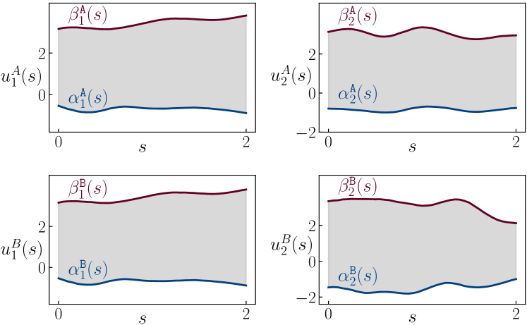
Let us consider two integrator agents A and B with relative degrees $\bm{r}^{\texttt{A}}=\bm{r}^{\texttt{B}}=(3,2)^{\top}$ as in (11), starting from respective initial conditions

$$\bm{x}_{0}^{\texttt{A}}=(0.5,\bm{0}_{{\small{1\times 4}}})^{\top},\quad\bm{x}_{0}^{\texttt{B}}=(\bm{0}_{{\small{1\times 3}}},5,0)^{\top}.$$

Given two box-valued input sets ๐’ฐAโ€‹(s)=[ฮฑ1Aโ€‹(s),ฮฒ1Aโ€‹(s)]ร—[ฮฑ2Aโ€‹(s),ฮฒ2Aโ€‹(s)]superscript๐’ฐA๐‘ superscriptsubscript๐›ผ1A๐‘ superscriptsubscript๐›ฝ1A๐‘ superscriptsubscript๐›ผ2A๐‘ superscriptsubscript๐›ฝ2A๐‘ \mathcal{U}^{\texttt{A}}(s)=[\alpha_{1}^{\texttt{A}}(s),\beta_{1}^{\texttt{A}}(s)]\times[\alpha_{2}^{\texttt{A}}(s),\beta_{2}^{\texttt{A}}(s)] and ๐’ฐBโ€‹(s)=[ฮฑ1Bโ€‹(s),ฮฒ1Bโ€‹(s)]ร—[ฮฑ2Bโ€‹(s),ฮฒ2Bโ€‹(s)]superscript๐’ฐB๐‘ superscriptsubscript๐›ผ1B๐‘ superscriptsubscript๐›ฝ1B๐‘ superscriptsubscript๐›ผ2B๐‘ superscriptsubscript๐›ฝ2B๐‘ \mathcal{U}^{\texttt{B}}(s)=[\alpha_{1}^{\texttt{B}}(s),\beta_{1}^{\texttt{B}}(s)]\times[\alpha_{2}^{\texttt{B}}(s),\beta_{2}^{\texttt{B}}(s)] shown in Fig. 1, we want to check if there is an intersection at time $t=2$ between the reach sets of agent A, denoted as $\mathcal{X}_{t}^{\texttt{A}}$, and that of agent B, denoted as $\mathcal{X}_{t}^{\texttt{B}}$.

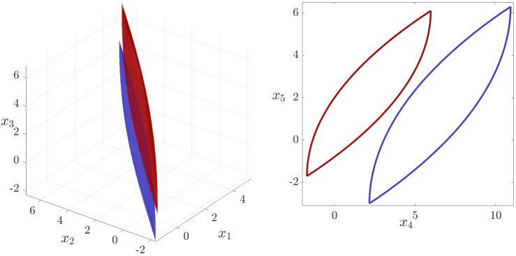
As explained in Sec. V-A, it suffices to check if there will be an intersection between each corresponding $j$th single input reach sets $\mathcal{X}_{jt}^{\texttt{A}}$ and $\mathcal{X}_{jt}^{\texttt{B}}$, for $j\in\{1,2\}$.

Using (48), we construct the matrices $\bm{M}_{j}^{i,{\tiny{\textup{box}}}},\bm{N}_{j}^{i,{\tiny{\textup{box}}}}$ and the vector $\bm{\kappa}_{j}^{i{\tiny{\textup{box}}}}$ for $i\in\{\texttt{A},\texttt{B}\}$. Then, we solve the optimization problems (47) for each $j\in\{1,2\}$ via MATLAB CVX toolbox [15, 16] with ฮ”โ€‹s=0.05ฮ”๐‘ 0.05\Delta s=0.05. The runtimes are $0.38$ s and $0.37$ s for $j=1$ and $j=2$, respectively. The corresponding optimal values are

$\displaystyle(\tilde{p}_{1}^{*},\tilde{p}_{2}^{*})=(0,-0.54).$ (49)

These optimal values imply ๐’ณ1โ€‹tAโˆฉ๐’ณ1โ€‹tBโ‰ โˆ…superscriptsubscript๐’ณ1๐‘กAsuperscriptsubscript๐’ณ1๐‘กB\mathcal{X}_{1t}^{\texttt{A}}\cap\mathcal{X}_{1t}^{\texttt{B}}\neq\varnothing, and $\mathcal{X}_{2t}^{\texttt{A}}\cap\mathcal{X}_{2t}^{\texttt{B}}=\varnothing$. Therefore, we conclude: $\mathcal{X}_{t}^{\texttt{A}}\cap\mathcal{X}_{t}^{\texttt{B}}=\varnothing$. The same pair (49) was obtained for smaller step-sizes:

  • โ€ข

    ฮ”โ€‹s=0.01ฮ”๐‘ 0.01\Delta s=0.01, runtimes are 0.80 s for both $j=1$ and $2$.

  • โ€ข

    ฮ”โ€‹s=0.005ฮ”๐‘ 0.005\Delta s=0.005, runtimes are 1.24 s and 1.25 s for $j=1$ and $j=2$, respectively.

In agreement with Theorem 4, for $\tilde{p}_{1}^{*}=0$, CVX returns $\|\bm{N}_{1}\bm{\eta}_{1}\|_{2}=0$, while for $\tilde{p}_{2}^{*}<0$, it returns $\|\bm{N}_{2}\bm{\eta}_{2}\|_{2}=1$ demonstrating that the convexification (47c) is lossless. This scenario is illustrated in Fig. 2.

VI Conclusions

This work presents a variational formulation for certifying or falsifying intersection of the reach sets of integrator agents subject to set-valued input uncertainties. The proposed nonconvex formulation is shown to enjoy lossless convexification for time-varying norm bounded as well as generic hyperrectangular input uncertainties, thus being amenable to convex programming for tractable computation. A numerical example is provided to illustrate the results.

-A Proof of Proposition 1

Support function is distributive over sum, so from (12) and (16), we obtain

$\displaystyle h_{\mathcal{X}_{t}}\left(\bm{y}\right)=$ โŸจ๐’š,expโก(tโ€‹๐‘จ)โ€‹๐’™0โŸฉ+hโˆซ0texpโก(sโ€‹๐‘จ)โ€‹๐‘ฉโ€‹๐’ฐโ€‹(s)โ€‹dsโ€‹(๐’š).๐’š๐‘ก๐‘จsubscript๐’™0subscriptโ„Žsuperscriptsubscript0๐‘ก๐‘ ๐‘จ๐‘ฉ๐’ฐ๐‘ differential-d๐‘ ๐’š\displaystyle\langle\bm{y},\exp\left(t\bm{A}\right)\bm{x}_{0}\rangle+h_{\int_{0}^{t}\exp(s\bm{A})\bm{B}\>\mathcal{U}(s)\>{\rm{d}}s}(\bm{y}). (50)

Using [17, Proposition 1], we then have

hโˆซ0texpโก(sโ€‹๐‘จ)โ€‹๐‘ฉโ€‹๐’ฐโ€‹(s)โ€‹dsโ€‹(๐’š)=โˆซ0thexpโก(sโ€‹๐‘จ)โ€‹๐‘ฉโ€‹๐’ฐโ€‹(s)โ€‹(๐’š)โ€‹dssubscriptโ„Žsuperscriptsubscript0๐‘ก๐‘ ๐‘จ๐‘ฉ๐’ฐ๐‘ differential-d๐‘ ๐’šsuperscriptsubscript0๐‘กsubscriptโ„Ž๐‘ ๐‘จ๐‘ฉ๐’ฐ๐‘ ๐’šdifferential-d๐‘ \displaystyle h_{\int_{0}^{t}\exp(s\bm{A})\bm{B}\>\mathcal{U}(s)\>{\rm{d}}s}(\bm{y})=\int_{0}^{t}\!\!h_{\exp(s\bm{A})\bm{B}\>\mathcal{U}(s)}\>(\bm{y})\;{\rm{d}}{s}
=โˆซ0tsup๐’–โ€‹(s)โˆˆ๐’ฐโ€‹(s)โ€‹โŸจ๐’š,expโก(sโ€‹๐‘จ)โ€‹๐‘ฉโ€‹๐’–โ€‹(s)โŸฉโ€‹ds.absentsuperscriptsubscript0๐‘ก๐’–๐‘ ๐’ฐ๐‘ supremum๐’š๐‘ ๐‘จ๐‘ฉ๐’–๐‘ differential-d๐‘ \displaystyle\qquad\qquad=\int_{0}^{t}\!\!\underset{\bm{u}(s)\in\mathcal{U}(s)}{\sup}\!\langle\bm{y},\exp(s\bm{A})\bm{B}\bm{u}(s)\rangle~{}{\rm{d}}s. (51)

Combining (-A) with the structures of the state and input matrices in (12)-(13), allows us to rewrite (50) as (1). Specifically, the result follows from the fact that the state transition matrix expโก(sโ€‹๐‘จ)=bldiagโ€‹(expโก(sโ€‹๐‘จ1),โ€ฆ,expโก(sโ€‹๐‘จm))๐‘ ๐‘จbldiag๐‘ subscript๐‘จ1โ€ฆ๐‘ subscript๐‘จ๐‘š\exp(s\bm{A})=\mathrm{bldiag}\left(\exp(s\bm{A}_{1}),\ldots,\exp(s\bm{A}_{m})\right) wherein each diagonal block is upper triangular with entries

(expโก(sโ€‹๐‘จj))aโ€‹b={saโˆ’b(aโˆ’b)!forโ€‹aโ‰คb,0otherwise,subscript๐‘ subscript๐‘จ๐‘—๐‘Ž๐‘casessuperscript๐‘ ๐‘Ž๐‘๐‘Ž๐‘for๐‘Ž๐‘0otherwise\left(\exp(s\bm{A}_{j})\right)_{ab}=\begin{cases}\dfrac{s^{a-b}}{(a-b)!}&\text{for}\;a\leq b,\\ 0&\text{otherwise},\end{cases}

for all $a,b=1,\ldots,r_{j}$, for each $j\in[m]$. โˆŽ

-B Proof of Theorem 1

Let ๐’›โ€‹(s):=(expโก(sโ€‹๐‘จ)โ€‹๐‘ฉ)โŠคโ€‹๐’šassign๐’›๐‘ superscript๐‘ ๐‘จ๐‘ฉtop๐’š\bm{z}(s):=(\exp(s\bm{A})\bm{B})^{\top}\bm{y} for all 0โ‰คsโ‰คt0๐‘ ๐‘ก0\leq s\leq t. Then, the integrand of the RHS of (-A) for time-varying $p$-norm ball input set ๐’ฐโ€‹(s)๐’ฐ๐‘ \mathcal{U}(s) as in (33), becomes

sup๐’–โ€‹(s)โˆˆโ„mโŸจ๐’›โ€‹(s),๐’–โ€‹(s)โŸฉ๐’–๐‘ superscriptโ„๐‘šsupremum๐’›๐‘ ๐’–๐‘ \displaystyle\underset{\bm{u}(s)\in\mathbb{R}^{m}}{\sup}\quad\>\langle\bm{z}(s),\bm{u}(s)\rangle
subject toโ€–๐’–โ€‹(s)โ€–pโ‰คโ„“โ€‹(s).subject tosubscriptnorm๐’–๐‘ ๐‘โ„“๐‘ \displaystyle\text{subject to}\quad\|\bm{u}(s)\|_{p}\leq\ell(s). (52)

Recall that $\|\cdot\|_{q}$ is the dual norm of $\|\cdot\|_{p}$ for $\frac{1}{p}+\frac{1}{q}=1$. From the definition of dual norm, we have

โŸจ๐’›โ€‹(s),๐’–โ€‹(s)โŸฉโ‰คโ€–๐’›โ€‹(s)โ€–qโ€‹โ€–๐’–โ€‹(s)โ€–pโ€‹โ‰ค(โ€‹52โ€‹)โ€‹โ„“โ€‹(s)โ€‹โ€–๐’›โ€‹(s)โ€–q๐’›๐‘ ๐’–๐‘ subscriptnorm๐’›๐‘ ๐‘žsubscriptnorm๐’–๐‘ ๐‘italic-(52italic-)โ„“๐‘ subscriptnorm๐’›๐‘ ๐‘ž\langle\bm{z}(s),\bm{u}(s)\rangle\leq\|\bm{z}(s)\|_{q}\|\bm{u}(s)\|_{p}\overset{\eqref{LP}}{\leq}\ell(s)\|\bm{z}(s)\|_{q}

with equality resulting in the supremum in (52). Substituting this supremum in (-A) and then using (50), we get (34). โˆŽ

-C Proof of Theorem 2

(i) Follows immediately from (37), (38) and (35).

(ii) Since $\bm{0}_{n\times 1}$ is in the feasible set of (35) and makes the objective equal to zero, we have $\tilde{p}^{*}\leq 0$.

(iii) Since $\tilde{p}^{*}$ is the optimal value of the convex relaxation of a nonconvex problem with optimal value $p^{*}$, we must have $\tilde{p}^{*}\leq p^{*}$. Thus, $\tilde{p}^{*}=0\Rightarrow 0\leq p^{*}$. That $0\leq p^{*}$ is equivalent to ๐’ณtAโˆฉ๐’ณtBโ‰ โˆ…superscriptsubscript๐’ณ๐‘กAsuperscriptsubscript๐’ณ๐‘กB\mathcal{X}_{t}^{\texttt{A}}\cap\mathcal{X}_{t}^{\texttt{B}}\neq\varnothing, was explained before in Sec. III.

(iv) We now show that when $\tilde{p}^{*}<0$, the convexification is in fact lossless, i.e., $\tilde{p}^{*}=p^{*}$. Denote the $\arg\min$ for the convex problem (35) as $\bm{y}^{\min}$. It suffices to prove that $\|\bm{y}^{\min}\|_{2}=1$. To this end, suppose if possible, that $\|\bm{y}^{\min}\|_{2}=:\delta<1$, i.e., $0<\delta<1$. Now let $\widetilde{\bm{y}}:=\bm{y}^{\min}/\delta$, which is clearly feasible w.r.t. (35). However,

$$f_{0}\left(\widetilde{\bm{y}}\right)=\underbrace{\frac{1}{\delta}}_{>1}\underbrace{\vphantom{\frac{1}{\varepsilon}}f_{0}(\bm{y}^{\min})}_{<0}<f_{0}(\bm{y}^{\min}),$$

contradicting the supposition that the $\arg\min$ is strictly within the unit ball in $\mathbb{R}^{n}$. Therefore, if $\tilde{p}^{*}<0$ then $\tilde{p}^{*}={p}^{*}$. That $p^{*}<0\Leftrightarrow\mathcal{X}_{t}^{\texttt{A}}\cap\mathcal{X}_{t}^{\texttt{B}}=\varnothing$, was explained in Sec. III. โˆŽ

-D Proof of Theorem 3

Specializing (1) for the box-valued input set (V), for all $j\in[m]$, we get

$\displaystyle h_{\mathcal{X}_{jt}}\left(\bm{y}_{j}\right)$ =โŸจ๐’šj,expโก(sโ€‹๐‘จj)โ€‹๐’™jโ€‹0โŸฉabsentsubscript๐’š๐‘—๐‘ subscript๐‘จ๐‘—subscript๐’™๐‘—0\displaystyle=\langle\bm{y}_{j},\exp\left(s\bm{A}_{j}\right)\bm{x}_{j0}\rangle
+โˆซ0tsupujโ€‹(s)โˆˆ[ฮฑjโ€‹(s),ฮฒjโ€‹(s)]โ€‹โŸจ๐’šj,๐ƒjโ€‹(s)โŸฉโ€‹ujโ€‹(s)โ€‹ds.subscriptsuperscript๐‘ก0subscript๐‘ข๐‘—๐‘ subscript๐›ผ๐‘—๐‘ subscript๐›ฝ๐‘—๐‘ supremumsubscript๐’š๐‘—subscript๐ƒ๐‘—๐‘ subscript๐‘ข๐‘—๐‘ differential-d๐‘ \displaystyle+\int^{t}_{0}\underset{u_{j}(s)\in\mathcal{[}\alpha_{j}(s),\beta_{j}(s)]}{\sup}\langle\bm{y}_{j},\bm{\xi}_{j}(s)\rangle\>u_{j}(s)\>{\rm{d}}{s}. (53)

The optimizer of the integrand in the RHS of (53), $u_{j}^{\text{opt}}$, can be written in terms of the Heaviside unit step function $H(\cdot)$ as

$\displaystyle u_{j}^{\text{opt}}$ $\displaystyle=\alpha_{j}+(\beta_{j}-\alpha_{j})H(\langle\bm{y}_{j},\bm{\xi}_{j}\rangle)$
$\displaystyle=\alpha_{j}+(\beta_{j}-\alpha_{j})\times\frac{1}{2}\left(1+{\rm{sgn}}\left(\langle\bm{y}_{j},\bm{\xi}_{j}\rangle\right)\right),$ (54)

where ${\rm{sgn}}(\cdot)$ denotes the sign function. Substituting the optimizer (54) into (53) yields (43). โˆŽ

References

  • [1] P.ย Varaiya, โ€œReach set computation using optimal control,โ€ in Verification of Digital and Hybrid Systems.ย ย ย Springer, 2000, pp. 323โ€“331.
  • [2] J.ย Yong and X.ย Y. Zhou, Stochastic controls: Hamiltonian systems and HJB equations.ย ย ย Springer Science & Business Media, 1999, vol.ย 43.
  • [3] Y.ย Cao, D.ย Stuart, W.ย Ren, and Z.ย Meng, โ€œDistributed containment control for multiple autonomous vehicles with double-integrator dynamics: algorithms and experiments,โ€ IEEE Transactions on Control Systems Technology, vol.ย 19, no.ย 4, pp. 929โ€“938, 2010.
  • [4] A.ย Abdessameud and A.ย Tayebi, โ€œOn consensus algorithms design for double integrator dynamics,โ€ Automatica, vol.ย 49, no.ย 1, pp. 253โ€“260, 2013.
  • [5] S.ย Li, H.ย Du, and X.ย Lin, โ€œFinite-time consensus algorithm for multi-agent systems with double-integrator dynamics,โ€ Automatica, vol.ย 47, no.ย 8, pp. 1706โ€“1712, 2011.
  • [6] A.ย Ajorlou and A.ย G. Aghdam, โ€œA bounded connectivity preserving aggregation strategy with collision avoidance property for single-integrator agents,โ€ in 2012 IEEE 51st IEEE Conference on Decision and Control (CDC).ย ย ย IEEE, 2012, pp. 4003โ€“4008.
  • [7] J.-B. Hiriart-Urruty and C.ย Lemarรฉchal, Convex analysis and minimization algorithms I: Fundamentals.ย ย ย Springer Science & Business media, 2013, vol. 305.
  • [8] R.ย Schneider, Convex bodies: the Brunnโ€“Minkowski theory.ย ย ย Cambridge university press, 2014, no. 151.
  • [9] L.ย Montejano, โ€œSome results about Minkowski addition and difference,โ€ Mathematika, vol.ย 43, no.ย 2, pp. 265โ€“273, 1996.
  • [10] Y.ย Zheng and K.ย Yamane, โ€œGeneralized distance between compact convex sets: Algorithms and applications,โ€ IEEE Transactions on Robotics, vol.ย 31, no.ย 4, pp. 988โ€“1003, 2015.
  • [11] S.ย Hornus, โ€œDetecting the intersection of two convex shapes by searching on the 2-sphere,โ€ Computer-Aided Design, vol.ย 90, pp. 71โ€“83, 2017.
  • [12] A.ย Lin and S.-P. Han, โ€œOn the distance between two ellipsoids,โ€ SIAM Journal on Optimization, vol.ย 13, no.ย 1, pp. 298โ€“308, 2002.
  • [13] S.ย Iwata, Y.ย Nakatsukasa, and A.ย Takeda, โ€œComputing the signed distance between overlapping ellipsoids,โ€ SIAM Journal on Optimization, vol.ย 25, no.ย 4, pp. 2359โ€“2384, 2015.
  • [14] S.ย Haddad and A.ย Halder, โ€œThe curious case of integrator reach sets, Part I: Basic theory,โ€ arXiv preprint arXiv:2102.11423, 2021.
  • [15] M.ย Grant and S.ย Boyd, โ€œCVX: Matlab software for disciplined convex programming, version 2.1,โ€ http://cvxr.com/cvx, Mar. 2014.
  • [16] โ€”โ€”, โ€œGraph implementations for nonsmooth convex programs,โ€ in Recent Advances in Learning and Control, ser. Lecture Notes in Control and Information Sciences, V.ย Blondel, S.ย Boyd, and H.ย Kimura, Eds.ย ย ย Springer-Verlag Limited, 2008, pp. 95โ€“110, http://stanford.edu/~boyd/graph_dcp.html.
  • [17] S.ย Haddad and A.ย Halder, โ€œThe convex geometry of integrator reach sets,โ€ in 2020 American Control Conference (ACC).ย ย ย IEEE, 2020, pp. 4466โ€“4471.