Sequential Bayesian Registration for Functional Data

Abstract

In many modern applications, discretely-observed data may be naturally understood as a set of functions. Functional data often exhibit two confounded sources of variability: amplitude ($y$-axis) and phase ($x$-axis). The extraction of amplitude and phase, a process known as registration, is essential in exploring the underlying structure of functional data in a variety of areas, from environmental monitoring to medical imaging. Critically, such data are often gathered sequentially with new functional observations arriving over time. Despite this, most available registration procedures are only applicable to batch learning, leading to inefficient computation. To address these challenges, we introduce a Bayesian framework for sequential registration of functional data, which updates statistical inference as new sets of functions are assimilated. This Bayesian model-based sequential learning approach utilizes sequential Monte Carlo sampling to recursively update the alignment of observed functions while accounting for associated uncertainty. As a result, distributed computing, which is not generally an option in batch learning, significantly reduces computational cost. Simulation studies and comparisons to existing batch learning methods reveal that the proposed approach performs well even when the target posterior distribution has a challenging structure. We apply the proposed method to three real datasets: (1) functions of annual drought intensity near Kaweah River in California, (2) annual sea surface salinity functions near Null Island, and (3) PQRST complexes segmented from an electrocardiogram signal.

Keywords Bayesian updating  $\cdot$ Amplitude  $\cdot$ Phase  $\cdot$ Function registration  $\cdot$ Sequential Monte Carlo  $\cdot$ Square-root velocity function

1 Introduction

In various real world problems, the goal of statistical analysis is to discover and explore patterns in the trajectories formed by the temporal evolution of a variable of interest. This type of data is commonly referred to as functional data, and is often recorded on a very fine temporal grid. The use of multivariate statistical methods to analyze functional data is inappropriate for two main reasons: (1) failure to account for the underlying infinite-dimensional structure of the data, and (2) inability to appropriately model strong temporal dependence within each functional observation [1, 2]. This has given rise to the field of functional data analysis (FDA), which provides a comprehensive framework for statistical modeling, summarization, analysis and visualization of data that comes in the form of functions [3, 4].

An important and common feature of functional data is that sampling is often automated or conducted over long periods of time, so that new functional data observations arrive sequentially. In general, there are two different approaches to perform statistical analysis for such an expanding collection of data in the finite or infinite-dimensional settings. The first is to implement the full spectrum of statistical analysis every time a new observation arrives, referred to as batch learning. The second is to exploit the existing analysis and update it by accounting for new data, referred to as sequential learning which is also known as online learning [5]. Most existing FDA techniques are designed for batch learning, meaning that they are performed once a given number of functional data is collected, and the analysis must be repeated on the entire sample as more data arrives. This fails to account for the sequential way in which functional data is often gathered, with the sample size increasing over time in many application domains such as environmental monitoring or biomedical imaging. For example, trajectories of annual temperature, or other measures related to the environment, are formulated through sets of repeated measurements on an annual basis; in medicine, biosignals such as electrocardiogram (ECG) signals or gait measurements contain repetitions of a particular pattern, e.g., the PQRST complex in ECG data, wherein each repetition can be interpreted as an observation. We provide a visualization of the example on sequential learning of trajectories of annual drought intensity in Figure 1. In such scenarios, new functional observations are added to existing data sequentially, so the statistical analysis pipeline must be modified to allow for updating and monitoring of inferential results as the collection of data expands.

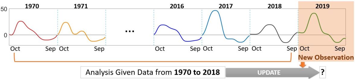
Figure 1: A visualization of sequential learning of functional data observed in a sequential manner. Trajectories of annual drought intensity measurements near Kaweah River in California recorded from 1970 to 2019.

1.1 Sequential learning

A sequential learning method seeks to update current inferential results based on new data. The Bayesian approach is well-suited to this problem because it (1) provides a systematic way to assimilate new data by updating the posterior distribution as new data arrives, and (2) allows the user to keep track of structured uncertainty. In most scenarios of interest, the posterior distribution does not have a closed form, so inference is based on estimates of posterior features obtained from posterior samples. Perhaps the most widely used sampling-based method for Bayesian inference is Markov chain Monte Carlo (MCMC), which is an example of a batch learning algorithm; as such, every time new data arrives, MCMC sampling must be repeated using the full data, resulting in inefficient computation. On the other hand, sequential Bayesian learning via, for example, sequential Monte Carlo (SMC) can assimilate new data as it arrives. Unlike MCMC, which targets a fixed posterior density, SMC defines a sequence of intermediate target densities, each being represented with a set of weighted particles that are perturbed and reweighted to represent the next density in the sequence [6, 7, 8]. When a subset of these intermediate target densities correspond to posteriors under different data availability scenarios, SMC becomes a sequential learning algorithm.

In addition to the efficiency of updating inference sequentially as new data arrives, SMC has two major advantages over sampling methods for batch learning, including MCMC. First, because each weighted SMC particle is treated independently, distributed computing can be used to substantially speed up its computational implementation. Second, compared to MCMC, SMC performs well for sampling from complex target posterior distributions, e.g., in the presence of multimodality, because the intermediate sequence of target densities can act as a bridge between the prior and a challenging posterior [9, 10, 11]. The potential for particle degeneracy, the phenomenon of particle weights becoming very small in certain situations and leading to large sampling variance in the SMC estimator, can be ameliorated through resampling or via MCMC-derived techniques such as block sampling [12, 13, 14, 15, 16]. While most existing SMC methods for sequential Bayesian learning are limited to multivariate data [8, 17], our focus in this work is on a natural inferential problem arising in FDA as described next.

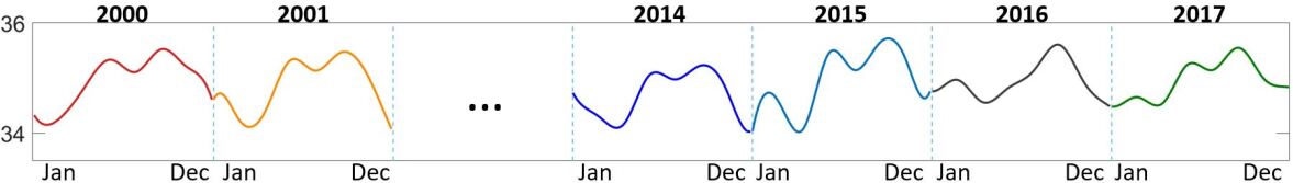
Figure 2: Sea surface salinity functions recorded near Null Island during 2000-2017.

1.2 Functional data registration

A common challenge in FDA is the presence of two confounded sources of variability termed amplitude and phase [18]. Examining Figure 2, which displays sea surface salinity (SSS) functions recorded near Null Island between the years 2000 and 2017, we note that the functions contain similar shape features, e.g., number of local extrema, but the timing of the features is not aligned along the temporal $x$-axis across all observations. For example, SSS tends to decrease early on each year following a small peak. Then, around the month of April, SSS increases sharply, which is followed by a bimodal pattern. While these features are common across most observations, they do not occur at the same time during the calendar year. Thus, the variation in the data can be attributed to two sources: (1) the magnitude of the measured values (SSS) termed amplitude or $y$-axis variability, and (2) the timing of amplitude features termed phase or $x$-axis variability. Phase variation may either be an inherent feature of data or the result of measurement error, and can be regarded as nuisance or a quantity of interest depending on the application. Importantly, phase variation cannot be ignored when performing statistical analysis of functional data as this may lead to misleading results [19]. Instead, the amplitude and phase components of functions should first be estimated through a process called registration. A common approach to registration is to consider the observed functions as deformed versions of an unknown template function (mean), and to extract their phase components via horizontal synchronization to an estimate of this template.

There are many methods for functional data registration [18, 20, 21]. Here, we briefly review a small subset. Landmark-based registration focuses on synchronization of (a small number of) landmarks, which represent important features of the observed functions, e.g., local extrema [4, 22]. While conceptually simple, these approaches rely on a faithful specification of landmarks, which is often difficult and time consuming. Metric-based registration utilizes a distance on the function space of interest to achieve horizontal synchronization of entire functions, i.e., it does not require landmark specification. However, the choice of distance is important as it must satisfy a key invariance property (see Section 2 for details). The standard $\mathbb{L}^{2}$ distance, which is commonly used in FDA, does not satisfy this property, and thus is inappropriate for metric-based registration. As an alternative, Srivastava et al. proposed the extended Fisher-Rao (eFR) Riemannian metric, which does satisfy this invariance property; unfortunately, the resulting distance is not computable in closed form [21]. However, a simple transformation of functional data, termed the square-root velocity function, simplifies the complicated eFR distance to the simple $\mathbb{L}^{2}$ distance, facilitating efficient computation. The resulting metric-based registration method is commonly referred to as elastic. Bayesian model-based registration of functional data has been explored relatively recently. In this setting, the main challenge lies in specifying an appropriate prior distribution over the phase component of functional data. Telesca and Inoue were the first to approach registration from this perspective and modeled phase via penalized B-splines [25]. Lu et al. explicitly considered the geometry of the representation space of the phase component and specified a Gaussian process prior on this space [26]. Horton et al. also modeled phase via a Gaussian process, but additionally allowed the incorporation of landmark information in the registration process [27]. Finally, Cheng et al., and Bharath and Kurtek used the Dirichlet distribution as a prior model on consecutive increments of discretized phase functions [28, 29]. An extension of Bayesian registration to sparse or fragmented functional data was recently developed by Matuk et al. [30]. Importantly, all of the aforementioned model-based approaches rely on batch learning, and in particular MCMC, for inference.

1.3 Contributions

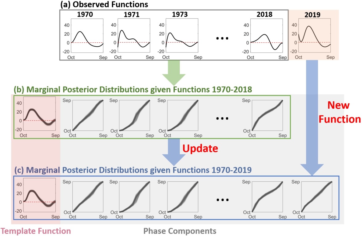
Figure 3: Illustration of results generated via the proposed sequential Bayesian registration method. (a) Functions of annual drought intensity measurements near Kaweah River in California recorded from 1970 to 2019. (b) The weighted samples (black; transparency reflects the magnitude of the weight of each sample) show posterior uncertainty over the template function (first column) and the phase components (second to fifth columns) given functions of annual drought intensities from 1970 to 2018. (c) Updated weighted samples show posterior uncertainty over the template function (first column) and the phase components (second to sixth columns) given functions of annual drought intensities from 1970 to 2019.

Motivated by data collection scenarios such as the one presented in Figure 1, we propose a novel sequential Bayesian learning approach for registration of functional data. To the best of our knowledge, this is the first sequential inference strategy for this statistical problem. The data-generating model we consider is built on the state-of-the-art framework proposed by Lu et al., where a template function and individual phase components constitute the parameters of interest [26]. Rather than specifying a Gaussian process prior on phase, we use the simpler and lower-dimensional Dirichlet distribution as a prior model on consecutive increments of discretized phase functions [29]. In this setting, the estimated phase components are piecewise linear functions resulting in improved interpretability of phase variation among functional data. The proposed sequential learning framework leverages SMC to efficiently update the joint posterior distribution over the template function and the phase components associated with each observation based on new data. We further address the challenge posed by the increasing dimension of the state space as new data is observed. In particular, each new function that is introduced as data has a corresponding phase component, which must be estimated, with respect to the template function. As a new function is observed, the state space is augmented to account for its associated phase component. Independently for each existing SMC particle, the new phase component is initialized by registering the new function relative to the particle’s template function component via a deterministic eFR metric-based registration approach. The particle weight is then updated while accounting for the increased state space dimension [31, 32]. The augmented weighted particles are then perturbed toward the next target posterior distribution using a Metropolis-Hastings kernel, and the weights are updated [14].

Results of the proposed approach are illustrated in Figure 3 using a real dataset of annual drought intensity near Kaweah River in California. Panel (a) displays functions of annual drought intensity from 1970 to 2018, denoted by $f_{1},\ldots,f_{n}$, as well as a new observation in 2019, $f_{n+1}$. The black bands in panel (b) provide a visualization of posterior uncertainty over the unknown template function and phase components given annual drought intensities from 1970 to 2018 based on a collection of weighted posterior samples, where line transparency is proportional to the magnitude of the weight. In the same manner, the plots in panel (c) summarize posterior uncertainty over the unknown template function and phase components updated from the posterior displayed in panel (b) accounting for the new annual drought intensity function observed in 2019.

The rest of this paper is organized as follows. Section 2 provides a brief review of elastic registration and SMC methods for state spaces of fixed as well as increasing dimension. Section 3 introduces the Bayesian registration model, while Section 4 describes the proposed SMC algorithm enabling sequential inference as new functional data is observed. Section 5 presents multiple simulations and real data examples. We implement the proposed registration approach to study trajectories of annual sea surface salinity near Null Island, trajectories of annual drought intensity near Kaweah River in California, and PQRST complexes segmented from a long electrocardiogram signal. We close with a brief summary and discussion of future work in Section 6.

2 Background material

In this section, we provide a brief review of the elastic registration framework [33], used to formulate our Bayesian registration model. We then review SMC methods for state spaces of fixed and increasing dimension [31, 14], which are adopted to perform sequential inference on the proposed model.

2.1 Elastic registration

Without loss of generality, we restrict our attention to absolutely continuous functions with domain $[0,1]$, resulting in the representation space $\mathcal{F}=\{f:[0,1]\rightarrow\mathbb{R}|f\textnormal{ is absolutely continuous}\}$. The phase component of a function $f\in\mathcal{F}$ is denoted by $\gamma$ and is an element of $\Gamma=\{\gamma:[0,1]\rightarrow[0,1]\mid\gamma(0)=0,\gamma(1)=1,0<\dot{\gamma}<\infty\}$, where $\dot{\gamma}$ is the time derivative of $\gamma$. The main goal of registration is to estimate the phase components $\gamma_{1},\dots,\gamma_{n}$ of a set of functions $f_{1},\ldots,f_{n}$, such that $f_{i}\circ\gamma_{i},\ i=1,\dots,n$ are horizontally synchronized, i.e., their features are well-aligned. The composition of $f$ and $\gamma$ is usually referred to as domain warping. Metric-based registration utilizes a distance on $\mathcal{F}$ to quantify the quality of alignment between two functions, and estimation of phase is carried out by minimizing this distance over elements of $\Gamma$. The chosen distance must satisfy $d(f_{1},f_{2})=d(f_{1}\circ\gamma,f_{2}\circ\gamma)$ for $f_{1},\ f_{2}\in\mathcal{F}$ and any $\gamma\in\Gamma$, i.e., it must be invariant to simultaneous domain warping. Crucially, the commonly used $\mathbb{L}^{2}$ distance does not satisfy this property.

Srivastava et al. proposed a formulation of metric-based registration using the extended Fisher-Rao (eFR) Riemannian metric [21]. The eFR distance is preserved under simultaneous domain warping, i.e., $d_{eFR}(f_{1},f_{2})=d_{eFR}(f_{1}\circ\gamma,f_{2}\circ\gamma)$ for $f_{1},\ f_{2}\in\mathcal{F}$ and any $\gamma\in\Gamma$. Since $d_{eFR}$, and thus the resulting registration problem, are not computationally tractable, Srivastava et al. introduced a transformation that allows the distance to be computed in closed form. The square-root velocity function (SRVF) representation given by the mapping $Q:\mathcal{F}\rightarrow\mathcal{Q}$ is defined as $Q(f)=\text{sign}(\dot{f})\sqrt{|\dot{f}|}:=q$ for $f\in\mathcal{F}$. Given the starting point $f(0)$, the mapping $Q$ is bijective and the original function can be reconstructed using $f(t)=Q^{-1}(f(0),q)(t)=f(0)+\int_{0}^{t}q(s)|q(s)|ds$. Further, under this mapping, the complicated eFR metric simplifies to the simple $\mathbb{L}^{2}$ metric, i.e., $d_{eFR}(f_{1},f_{2})=d_{\mathbb{L}^{2}}(Q(f_{1}),Q(f_{2}))$ for $f_{1},\ f_{2},\in\mathcal{F}$, and the resulting space of SRVFs $\mathcal{Q}$ is a subset of $\mathbb{L}^{2}([0,1],\mathbb{R})$. The domain warping $f\circ\gamma$ of a function $f\in\mathcal{F}$ via $\gamma\in\Gamma$ can be mapped to the SRVF space by the operation $(q,\gamma):=(q\circ\gamma)\sqrt{\dot{\gamma}}$ where $q=Q(f)$. Finally, the amplitude of a function $f$ can be formally defined through its SRVF $q$ as the equivalence class $[q]=\{(q,\gamma)\mid\gamma\in\Gamma\}$; the set of all amplitudes is the quotient space $\mathcal{Q}/\Gamma$.

The SRVF representation is then used to define the metric-based registration problem as follows. For registration of two functions, $f_{1},\ f_{2}\in\cal{F}$, we set $f_{1}$ as the reference function and find the optimal phase component of $f_{2}$ that minimizes the $\mathbb{L}^{2}$ distance between their SRVFs $q_{1},\ q_{2}\in\cal{Q}$, i.e., $\gamma=\arg\min_{\gamma\in\Gamma}d_{\mathbb{L}^{2}}(q_{1},(q_{2},\gamma))$. When multiple functions $f_{1},\ldots,f_{n}$ are given, we register them to (an estimate of) a representative of the mean equivalence class, referred to as a template, rather than an arbitrarily chosen reference function. The SRVF of the template function, denoted by $q_{\mu}$, is estimated using the so-called Karcher mean $[q_{\mu}]=\arg\min_{[q_{\mu}]\in\mathcal{Q}/\Gamma}\sum_{i=1}^{n}\min_{\gamma\in\Gamma}d_{\mathbb{L}^{2}}(q_{\mu},(q_{i},\gamma))^{2}$; the solution is an entire equivalence class. For identifiability, one generally selects $q_{\mu}\in[q_{\mu}]$ such that the average of the phase components, estimated via $\gamma_{i}=\arg\min_{\gamma\in\Gamma}d_{\mathbb{L}^{2}}(q_{\mu},(q_{i},\gamma))$, $i=1,\ldots,n$, is the identity $\gamma_{id}(t)=t$. For visualization, the SRVF of the template function, $q_{\mu}$, can be mapped to $\mathcal{F}$ using $Q^{-1}$.

2.2 Sequential Monte Carlo

Sequential Monte Carlo (SMC) refers to a class of sampling algorithms targeting a sequence of prespecified distributions [34]. In the Bayesian inferential setting, these consist of either a sequence of posterior distributions or some transformation thereof. Suppose the target distributions have densities $\eta_{\tau}$, $\tau\in\mathbb{N}_{+}$, over the state variables $\theta_{\tau}$. SMC is a sequential version of importance sampling that generates a set of weighted samples, which are used to approximate features of each intermediate target distribution. This allows the user to track uncertainty while updating inference recursively, or sequentially annealing challenging posterior distributions. For an intermediate probability density $\eta_{\tau}$, samples are first randomly drawn from a different distribution, termed the importance distribution with density denoted by $g_{\tau}$, which is easy to sample from and is available in closed form. These samples, also known as particles, are then re-weighted to reflect the shape of $\eta_{\tau}$. To make the description more precise, let $\theta_{\tau}^{(j)},\ j=1,\ldots,J$ represent $J$ samples drawn from the importance distribution. Then, their corresponding weights are computed as $w_{\tau}^{(j)}\propto\eta_{\tau}(\theta_{\tau}^{(j)})/g_{\tau}(\theta_{\tau}^{(j)})$ and subsequently normalized, so that the pairs $\{(\theta_{\tau}^{(j)},w_{\tau}^{(j)}),\ j=1,\ldots,J\}$ form a collection of weighted samples from $\eta_{\tau}(\cdot)$. Crucially, the next density $\eta_{\tau+1}$ in the sequence can then be sampled recursively starting from the weighted pairs from the importance density $g_{\tau+1}=\eta_{\tau}$, and so on. We present a brief overview of SMC for two different Bayesian inference scenarios: (1) a state space with increasing dimension and target distributions having fixed marginal densities across the sequence, and (2) a fixed-dimensional state space and subsequent target distributions that are similar.

2.2.1 SMC for state space with increasing dimension

SMC on a state space of increasing dimension is often of interest, e.g., when the target sequence of distributions consists of posteriors over an increasing number of unknown model components. Assume that we are given a set of weighted samples, $\{(\theta_{\tau}^{(j)},w_{\tau}^{(j)}),\ j=1,\ldots,J\}$, drawn from the distribution with density $\eta_{\tau}$, and we aim to modify the weights and particles such that they approximate the next target distribution in the sequence with density $\eta_{\tau+1}$. Suppose that the state variable $\theta_{\tau}$ at time $\tau+1$ is obtained by appending a new variable $\tilde{\theta}$ to the previous state so that $\theta_{\tau+1}=(\theta_{\tau},\tilde{\theta})$, and the marginal density of $\theta_{\tau}$ at time $\tau+1$ is equal to the density at time $\tau$, i.e., $\eta_{\tau}(\theta_{\tau})=\eta_{\tau+1}(\theta_{\tau})$. Interest lies in approximating $\eta_{\tau+1}$ using the pairs $\{(\theta_{\tau}^{(j)},w_{\tau}^{(j)}),\ j=1,\ldots,J\}$ as well as random samples from the conditional distribution of $\tilde{\theta}$ given $\theta_{\tau}$. Liu and Chen present an SMC sampler for such a scenario, which is described below [31].

Since the marginal distribution of $\theta_{\tau}$ does not change in this scenario from time $\tau$ to $\tau+1$, we may keep the existing sample and append new particles corresponding to $\tilde{\theta}$ generated through a Markov transition kernel ${K}_{\tau+1}$ such that ${K}_{\tau+1}(\theta_{\tau+1}\mid\theta_{\tau})={K}_{\tau+1}(\tilde{\theta}\mid\theta_{\tau})$ . An efficient choice for the transition kernel is one that targets the conditional distribution of $\tilde{\theta}$ given $\theta_{\tau}$. Then, the resulting augmented particles are $\theta_{\tau+1}^{(j)}=(\theta_{\tau}^{(j)},\tilde{\theta}^{(j)}),\ j=1,\ldots,J$. The unnormalized weights of $\theta_{\tau+1}^{(j)},\ j=1,\ldots,J$ are updated using (the superscript $(j)$ is omitted for brevity)

$$w_{\tau+1}\propto\frac{\eta_{\tau+1}\left(\theta_{\tau+1}\right)}{{g}_{\tau+1}\left(\theta_{\tau+1}\right)}=w_{\tau}\frac{\eta_{\tau+1}\left(\theta_{\tau+1}\right)}{\eta_{\tau}\left(\theta_{\tau}\right){K}_{\tau+1}\left(\tilde{\theta}\mid\theta_{\tau}\right)},$$ (1)

where ${g}_{\tau+1}$ denotes the importance density for sampling $\theta_{\tau+1}$; once computed, the weights can be normalized. This framework is widely used for dynamical systems with state space models increasing in dimension [31].

If we recursively update weighted samples for a long sequence of distributions with increasing state space dimension, at some point the weighted samples may poorly estimate the target distribution due to the curse of dimensionality. For example, when using $J$ weighted samples to approximate the target distribution at time $\tau$, fewer particles retain large weights as the dimension increases with $\tau$ for subsequent target distributions. This is known as the degeneracy problem. To measure potential degeneracy, we compute the effective sample size (ESS) using the magnitude of the normalized weights, $ESS=\left(\sum_{j=1}^{J}(w_{\tau}^{(j)})^{2}\right)^{-1}$. If ESS is small, a large portion of the weighted samples have small weights and the degeneracy issue is observed. One can address this problem by eliminating samples with low weights and duplicating the ones with large weights through resampling [12, 13]. A common approach draws random samples from the multinomial distribution with weights serving as parameters; the resampled particles are then assigned equal weights [35]. The overall procedure is as follows: (1) draw samples of $\tilde{\theta}$ through a Markov transition kernel $K_{\tau+1}$, (2) update the weights using Equation 1, and (3) resample the weighted samples if ESS $<J/2$.

2.2.2 SMC for state space with fixed dimension

Another scenario of interest is when the state space dimension is fixed, but intermediate distributions vary across a sequence. This occurs, for example, when we wish to sample from a challenging target posterior distribution by building a sequence, or bridge, of intermediate distributions that are similar to one another, such as annealed versions of the posterior density. Assume that we have a set of weighted samples from a distribution at time $\tau$ and we aim to perturb them toward the target distribution at time $\tau+1$. We assume that the dimensions of the state variables at times $\tau$ and $\tau+1$ are the same, i.e., $dim(\theta_{\tau})=dim(\theta_{\tau+1})$, and that the adjacent distributions are similar to each other, i.e., $\eta_{\tau}(\theta_{\tau})\approx\eta_{\tau+1}(\theta_{\tau+1})$. Given a set of weighted samples $\{(\theta_{\tau}^{(j)},w_{\tau}^{(j)}),\ j=1,\ldots,J\}$, sampled at time $\tau$, we perturb them toward the target distribution $\eta_{\tau+1}$ via a forward transition kernel, $K_{\tau+1}(\theta_{\tau+1}\mid\theta_{\tau})$. A natural choice of transition kernel in this case is an MCMC kernel. After perturbing the existing particles, we need to update their weights accordingly:

$$w_{\tau+1}\propto\frac{\eta_{\tau+1}(\theta_{\tau+1})}{g_{\tau+1}(\theta_{\tau+1})}=\frac{\eta_{\tau+1}(\theta_{\tau+1})}{\int g_{\tau}(\theta_{\tau})K_{\tau+1}(\theta_{\tau+1}\mid\theta_{\tau})d\theta_{\tau}}.$$ (2)

This requires us to update the importance density which is, however, often intractable as it involves integration that does not have a closed form solution.

To circumvent this issue, Del Moral et al. introduced the following approach [14]. First, existing particles are perturbed toward the target distribution $\eta_{\tau+1}$ through the forward transition kernel $K_{\tau+1}(\theta_{\tau+1}\mid\theta_{\tau})$. The updated weight for each particle may then be computed through the use of a backward kernel $L_{\tau}(\theta_{\tau}\mid\theta_{\tau+1})$ as (the superscript $(j)$ is omitted for brevity)

$$w_{\tau+1}\propto w_{\tau}\frac{\eta_{\tau+1}\left(\theta_{\tau+1}\right)L_{\tau}\left(\theta_{\tau}\mid\theta_{\tau+1}\right)}{\eta_{\tau}\left(\theta_{\tau}\right)K_{\tau+1}\left(\theta_{\tau+1}\mid\theta_{\tau}\right)},$$ (3)

but only if the transition kernel has a closed form. If $K_{\tau+1}$ is chosen to be an MCMC kernel that is invariant to $\eta_{\tau+1}$, and the adjacent target distributions are similar, Del Moral et al. proposed using the following approximate backward kernel that avoids explicit evaluation of $K_{\tau+1}$ and $L_{\tau}$ in the weight update [14],

$$L_{\tau}\left(\theta_{\tau}\mid\theta_{\tau+1}\right)=\frac{\eta_{\tau+1}\left(\theta_{\tau}\right)K_{\tau+1}\left(\theta_{\tau}\mid\theta_{\tau+1}\right)}{\eta_{\tau+1}\left(\theta_{\tau+1}\right)}.$$ (4)

For this choice of backward kernel, the weight update specified in Equation 3 simplifies to (the superscript $(j)$ is omitted for brevity)

$$w_{\tau+1}\propto w_{\tau}\frac{\eta_{\tau+1}(\theta_{\tau})}{\eta_{\tau}\left(\theta_{\tau}\right)},$$ (5)

which is easily computed. This approximated weight updating approach allows us to use transition kernels of which densities are intractable, e.g., a Metropolis-Hastings kernel requires integration which is not computable in closed form. The weights are subsequently normalized.

3 Bayesian model for registration of functional data

Here, we formulate a Bayesian hierarchical model for elastic registration of functions based on the SRVF representation. The choice of this representation is motivated by the desirable properties of the eFR metric as described in Section 2.1. The presented model is a modification of the model in [26] utilizing a more flexible choice of prior distribution over phase. We again denote the functional data by $f_{1},\ldots,f_{n}\in\mathcal{F}$ and the corresponding SRVFs by $q_{1},\ldots,q_{n}\in\mathcal{Q}$. We assume that each datum $f_{i}$ is a noisy deformation of a template function $f_{\mu}\in\mathcal{F}$, determined by the phase function $\gamma_{i}\in\Gamma$. The observation error is assumed to be additive in the SRVF space, yielding the observation model $q_{i}=(q_{\mu},\gamma_{i}^{-1})+\epsilon_{i},\ i=1,\dots,n$, where $q_{\mu}$ is the SRVF of the unknown template function, $\gamma_{i},\ i=1,\ldots,n$ are the phase components of the data, and $\epsilon_{i}$ is an error process in the SRVF space. Recall that the domain warping of a function $f\in\cal{F}$ via $\gamma\in\Gamma$ is $f\circ\gamma$, and its SRVF is given by $(q,\gamma)=(q\circ\gamma)\sqrt{\dot{\gamma}}$, where $q=Q(f)$. At the implementation stage, the functional data is discretized using evaluations on a finite grid of time points $[t]=\left(t_{1}=0,\ldots,t_{M}=1\right)^{\top}\in[0,1]^{M}$, where $t_{1}<t_{2}<\cdots<t_{M}$, leading to the discretized SRVFs $q_{i}([t]),\ i=1,\dots,n$. Assuming that the error follows a Gaussian process with white noise covariance structure leads to the following likelihood:

$$q_{i}([t])-(q_{\mu},\gamma_{i}^{-1})([t])|q_{\mu},\gamma_{i},\sigma^{2}\overset{iid}{\sim}N(0_{M},\sigma^{2}I_{M}),\quad i=1,\ldots,n,$$ (6)

where $0_{M}$ is an $M\times 1$ zero vector and $I_{M}$ is an $M\times M$ identity matrix.

Next, we specify prior distributions for the unknown parameters of interest $q_{\mu}$ and $\gamma_{i},\ i=1,\dots,n$ (and $\sigma^{2}$). We assume that the SRVF $q_{\mu}$ of the template function $f_{\mu}$ is a linear combination of $B$ orthonormal basis functions, so that $q_{\mu}(t)=\sum_{b=1}^{B}c_{b}\phi_{b}(t)$. The number and type of basis functions $\phi_{1},\ldots,\phi_{B}:[0,1]\rightarrow\mathbb{R}$ depend on the application of interest; specific choices are discussed in Section 5. We denote the vector of basis coefficients by $\textbf{c}=\left(c_{1},\ldots,c_{B}\right)^{\top}$ and assume a multivariate Gaussian prior on c: $\textbf{c}\sim N(0_{B},\Sigma_{c})$. This multivariate Gaussian prior on the basis coefficient vector corresponds to a Gaussian process prior on the (SRVF of the) template function, restricted to finite dimension corresponding to the number of basis elements $B$ [26]. Each phase component, $\gamma_{i}$, is an increasing function with $\gamma_{i}(0)=0$ and $\gamma_{i}(1)=1$. We adopt a prior model for phase based on a finite piecewise linear process introduced by Bharath and Kurtek [29]. While this model assumes that phase functions are piecewise linear, it is flexible enough to capture phase variation among functional data. The partition of the domain $[0,1]$ is prespecified as $0=s_{1}<s_{2}<\cdots<s_{M_{\gamma}-1}<s_{M_{\gamma}}=1$, with $M_{\gamma}$ denoting the size of the partition. Denote a vector of phase increments by $\textbf{d}=d(\gamma)=(\gamma(s_{2}),\ldots,\gamma(s_{m})-\gamma(s_{m-1}),\ldots,1-\gamma(s_{M_{\gamma}-1}))^{\top}$; the vector d uniquely represents $\gamma$ given the prespecified partition. The vector d is an element of the $(M_{\gamma}-1)$-dimensional simplex and we assign a Dirichlet distribution as a prior model over this space: $\textbf{d}|\textbf{u}\sim Dir\left(\kappa\textbf{u}\right)$, where $\textbf{u}=(u_{(1)},\ldots,u_{(m-1)}-u_{(m)},\ldots,1-u_{(M_{\gamma}-1)})^{\top}$ and $u_{(1)},\ldots,u_{(M_{\gamma}-1)}$ are order statistics of a random sample drawn from the uniform distribution on $[0,1]$. The flexibility of this prior model is determined by the partition size, $M_{\gamma}$, while $\kappa$ serves as a concentration parameter. The prior is centered around identity warping $\gamma_{id}$. The prior model for the error variance in the SRVF space, $\sigma^{2}$, is chosen to be an inverse gamma distribution, which is conjugate for the multivariate Gaussian likelihood.

The full Bayesian hierarchical model is given as follows:

$$q_{i}([t])-(q_{\mu},\gamma_{i}^{-1})([t])|q_{\mu},\gamma_{i},\sigma^{2} \overset{iid}{\sim}N(0_{M},\sigma^{2}I_{M}),\quad i=1,\ldots,n,$$

$$q_{\mu} =\sum_{b=1}^{B}c_{b}\phi_{b}$$

$$\gamma_{i} =d^{-1}(\textbf{d}_{i}),\quad i=1,\ldots,n$$

c $$\sim N(0_{B},\Sigma_{c}),$$

$$\textbf{d}_{i}|\textbf{u} \overset{iid}{\sim}Dir(\kappa\textbf{u}),\quad i=1,\ldots,n,$$

$$\sigma^{2} \sim IG(shape=\alpha_{\sigma},scale=\beta_{\sigma}),$$ (7)

where $\textbf{c},\textbf{d}_{1},\ldots,\textbf{d}_{n}$, and $\sigma^{2}$ are assumed to be independent a priori. We assume that $\Sigma_{c},\ \kappa,\ \alpha_{\sigma},$ and $\beta_{\sigma}$ are known.

4 Sequential Monte Carlo algorithm for registration of functional data

In this section, we present the proposed sequential Bayesian registration approach for the model introduced in Section 3, noting that it can be straightforwardly extended to a wider variety of models for functional data, for which the state space similarly increases in dimension as new data arrives. In the following, we will use the subscript $1:n$ to denote a set of objects indexed from $1$ through $n$, so that, for example, $f_{1:n}=\{f_{1},\ldots,f_{n}\}$ represents the first $n$ observed functions and $\textbf{d}_{1:n}=\{\textbf{d}_{1},\ldots,\textbf{d}_{n}\}$ represents the increments of the phase components for the first $n$ functions. Let $\ldots,\pi(\textbf{c},\textbf{d}_{1:n},\sigma^{2}\mid f_{1:n}),\ \pi(\textbf{c},\textbf{d}_{1:n+1},\sigma^{2}\mid f_{1:n+1}),\ \pi(\textbf{c},\textbf{d}_{1:n+2},\sigma^{2}\mid f_{1:n+2}),\ldots$ denote the sequence of target posterior densities of interest, and suppose that we have a large number of weighted samples $\{(\textbf{c}^{(j)},\textbf{d}^{(j)}_{1:n},\sigma^{2(j)},w^{(j)}),\ j=1,\ldots,J\}$ approximating the posterior $\pi(\textbf{c},\textbf{d}_{1:n},\sigma^{2}\mid f_{1:n})$, where c is the vector of basis coefficients defining the template function. The goal is to update these particles and weights to generate a new weighted sample $\{(\textbf{c}^{(j)},\textbf{d}^{(j)}_{1:n+1},\sigma^{2(j)},w^{(j)}),\ j=1,\ldots,J\}$, approximating the posterior $\pi(\textbf{c},\textbf{d}_{1:n+1},\sigma^{2}\mid f_{1:n+1})$, as a new function $f_{n+1}$ becomes part of the data.

The first step is to augment the previous particles with a phase component corresponding to the new function $f_{n+1}$. An important consideration for avoiding particle degeneracy when the state dimension increases is to ensure that the new components of each particle are initialized so that the sample lies in a region of relatively high posterior probability. In general, the marginal posterior distribution of c, $\textbf{d}_{1:n}$, and $\sigma^{2}$ given $f_{1:n}$ does not change very much when we observe a new function $f_{n+1}$, especially for large $n$. Thus, augmenting the existing particles $(\textbf{c}^{(j)},\textbf{d}_{1:n}^{(j)},\sigma^{2(j)})$ with a sensible initialization of $\textbf{d}_{n+1}^{(j)}$, for $j=1,\ldots,J$, results in a collection of particles that provide good coverage of the target posterior density $\pi(\textbf{c},\textbf{d}_{1:n+1},\sigma^{2}\mid f_{1:n+1})$. Since phase is a relative quantity with respect to the template function, we propose to initialize this new phase vector for each particle by registering $f_{n+1}$ to the template component of that particle. For this, we use the elastic registration approach with the template $q_{\mu}^{(j)}=\sum_{b=1}^{B}c_{b}^{(j)}\phi_{b}$, by solving the optimization problem ($q_{n+1}=Q(f_{n+1})$)

$$\hat{\gamma}^{(j)}=\arg\min_{\gamma\in\Gamma}\|q_{\mu}^{(j)}-(q_{n+1}\circ\gamma)\sqrt{\dot{\gamma}}\|^{2},$$ (8)

via the Dynamic Programming algorithm [32]. Each resulting $\hat{\gamma}^{(j)}$ is a piecewise linear function that is finely sampled on the domain $[0,1]$. To generate $\textbf{d}_{n+1}^{(j)}=d(\hat{\gamma}^{(j)})$, we further approximate $\hat{\gamma}^{(j)}$ over the prespecified partition $0=s_{1}<s_{2}<\ldots<s_{M_{\gamma}-1}<s_{M_{\gamma}}=1$ using a least squares procedure.

The next step is to update the weight of each particle while accounting for the increased dimension of the parameter space. We adopt the approach of [31] with a deterministic transition kernel to compute each weight $\tilde{w}^{(j)}$ as,

$$\tilde{w}^{(j)} \propto\frac{\pi\left(\textbf{c}^{(j)},\textbf{d}_{1:n+1}^{(j)},\sigma^{2(j)}\mid f_{1:n+1}\right)}{g\left(\textbf{c}^{(j)},\textbf{d}_{1:n+1}^{(j)},\sigma^{2(j)}\mid f_{1:n+1}\right)},$$ (9)

$$=\frac{h\left(f_{1:n+1}\mid\textbf{c}^{(j)},\textbf{d}_{1:n+1}^{(j)},\sigma^{2(j)}\right)p\left(\textbf{c}^{(j)},\textbf{d}_{1:n+1}^{(j)},\sigma^{2(j)}\right)}{g\left(\textbf{c}^{(j)},\textbf{d}_{1:n}^{(j)},\sigma^{2(j)}\mid f_{1:n}\right)K\left(\textbf{d}_{n+1}^{(j)}\mid\textbf{c}^{(j)},f_{n+1}\right)},$$

$$=w^{(j)}\frac{h\left(f_{n+1}\mid\textbf{c}^{(j)},\textbf{d}_{n+1}^{(j)},\sigma^{2(j)}\right)p\left(\textbf{d}_{n+1}^{(j)}\right)}{K\left(\textbf{d}^{(j)}_{n+1}\mid\textbf{c}^{(j)},f_{n+1}\right)},$$ (10)

$$=w^{(j)}h\left(f_{n+1}\mid\textbf{c}^{(j)},\textbf{d}_{n+1}^{(j)},\sigma^{2(j)}\right)p\left(\textbf{d}_{n+1}^{(j)}\right),$$ (11)

where $g$ is the importance sampling density, $h$ is the likelihood, $p$ is the prior density, and $K$ is the transition kernel density. The last equality holds because our initialization of $\textbf{d}^{(j)}_{n+1}$ is deterministic given $f_{n+1}$ and $\textbf{c}^{(j)}$, so the transition kernel is also deterministic and the kernel density $K(\textbf{d}^{(j)}_{n+1}\mid\textbf{c}^{(j)},f_{n+1})=1$. After these updates, we monitor the effective sample size $ESS=\left(\sum_{j=1}^{J}(\tilde{w}^{(j)})^{2}\right)^{-1}$, and resample the particles if ESS is smaller than the standard threshold of $J/2$. Resampling is performed using a multinomial distribution with parameters $\tilde{w}^{(j)},\ j=1,\ldots,J$, and we assign equal weights to the resampled particles.

While the resulting weighted samples $\{(\textbf{c}^{(j)},\textbf{d}^{(j)}_{1:n+1},\sigma^{2(j)},\tilde{w}^{(j)}),\ j=1,\ldots,J\}$ already approximate the target posterior $\pi(\textbf{c},\textbf{d}_{1:n+1},\sigma^{2}\mid f_{1:n+1})$, we perform an additional perturbation step to ensure that particles better represent the new target posterior. We find that this step guards against particle degeneracy in future updates. The perturbation of $\textbf{c}^{(j)}$ and $\textbf{d}_{1:n+1}^{(j)},\ j=1,\ldots,J,$ is performed via a Metropolis-Hastings (MH) transition kernel and the weights are updated. With a slight abuse in notation, let the updated particles of c and $\textbf{d}_{1:n+1}$ be denoted by $\{(\textbf{c}^{(j)},\textbf{d}^{(j)}_{1:n+1}),\ j=1,\ldots,J\}$. We adopt the approximate backward kernel approach introduced by Del Moral et al. to avoid computing the density of the MH kernels [14]. Since the MH kernel is invariant to $\pi(\textbf{c},\textbf{d}_{1:n+1},\sigma^{2}\mid f_{1:n+1})$, the weight update in Equation 5 simplifies to $\tilde{\tilde{w}}^{(j)}=\tilde{w}^{(j)}$ under the reasonable assumption that the marginal posteriors given $f_{1:n}$ and $f_{1:n+1}$ are similar. In other words, the weights are approximately invariant to the MH-based perturbation.

Additionally, after each full update, we perform a centering step to ensure identifiability of the template function (see Section 2.1 for a brief discussion). This step constrains the mean of the phase components of the data with respect to the template function to be the identity $\gamma_{id}$. To do this, we first compute the sample average of the phase components $\gamma_{1:n+1}^{(j)}=d^{-1}(\textbf{d}_{1:n+1}^{(j)})$ [21], and then apply its inverse to each template function $\mu_{q}^{(j)}=\sum_{b=1}^{B}c_{b}^{(j)}\phi_{b}$ and each phase $\gamma_{1:n+1}^{(j)}$. We then update the weights accordingly. As this step utilizes a deterministic kernel, and the importance density and likelihood are invariant to simultaneous warping, the weight update is based on the ratio of prior densities evaluated at the centered particles and their uncentered counterparts. To do this, we first use the centered template function and phase components to construct the centered particles $\{(\tilde{\textbf{c}}^{(j)},\tilde{\textbf{d}}_{n+1}^{(j)}),\ j=1,\ldots,J\}$. We then update the weights using

$$\tilde{w}^{(j)}\leftarrow\tilde{w}^{(j)}\frac{p(\tilde{\textbf{c}}^{(j)},\tilde{\textbf{d}}_{1:n+1}^{(j)})}{p(\textbf{c}^{(j)},\textbf{d}_{1:n+1}^{(j)})},$$ (12)

which are normalized subsequently. Assuming that the initial samples are centered (this is the standard approach in MCMC-based batch learning for registration of functional data [26, 28]), the sample average of the phase components does not deviate very much from the identity after each new function is observed. This fact, coupled with our specification of diffuse priors, ensures that the weights do not change much due to this centering step. As such, to improve computational efficiency of the proposed SMC algorithm, one may choose to not update the weights of the particles after the centering step.

Algorithm 1 Sequential Bayesian Registration Algorithm

1:Inputs:

2:      (1) SRVFs $q_{1:n+1}$ of $f_{1:n+1}$. (2) Posterior draws given $f_{1:n}$: $\{(\textbf{c}^{(j)},\textbf{d}_{1:n}^{(j)},\sigma^{2(j)},w^{(j)}),\ j=1,\ldots,J\}$.

3:Outputs:

4:      Posterior draws given $f_{1:n+1}$: $\{(\tilde{\textbf{c}}^{(j)},\tilde{\textbf{d}}_{1:n+1}^{(j)},\tilde{\sigma}^{2(j)},\tilde{w}^{(j)}),\ j=1,\ldots,J\}$.

5:for $j=1,\ldots,J$ do

6:     Compute $\hat{\gamma}^{(j)}\leftarrow\arg\min_{\gamma\in\Gamma}\|\sum_{b=1}^{B}c_{b}^{(j)}\phi_{b}-(q_{n+1}\circ\gamma)\sqrt{\dot{\gamma}}\|^{2}$ via Dynamic Programming.

7:     Approximate $\hat{\gamma}^{(j)}$ using a piecewise linear function evaluated at $(s_{1},s_{2},\ldots,s_{M_{\gamma}-1},s_{M_{\gamma}})$ via least squares, and compute $\textbf{d}_{n+1}^{(j)}=d(\hat{\gamma}^{(j)})$.

8:     Update the weights using $\tilde{w}^{(j)}\leftarrow w^{(j)}h(f_{n+1}|\textbf{c}^{(j)},\textbf{d}_{n+1}^{(j)},\sigma^{2(j)})p(\textbf{d}_{n+1}^{(j)}).$

9:end for

10:Normalize the weights, $[\tilde{w}^{(1)},\ldots,\tilde{w}^{(J)}]^{\top}\leftarrow\frac{1}{\sum_{j=1}^{J}\tilde{w}^{(j)}}[\tilde{w}^{(1)},\ldots,\tilde{w}^{(J)}]^{\top}$.

11:if $(\sum_{j=1}^{J}(\tilde{w}^{(j)})^{2})^{-1}<J/2$ then.

12:     Resample the particles using multinomial distribution with current weights as parameters, and assign equal weight to each resampled particle.

13:end if

14:Compute posterior covariance: $\hat{\Sigma}_{c}\leftarrow\frac{1}{J-1}\sum_{j=1}^{J}\tilde{w}^{(j)}\textbf{c}^{(j)}\textbf{c}^{(j)\top}$.

15:for $j=1,\ldots,J$ do

16:     $\gamma_{1:n+1}^{(j)}\leftarrow d^{-1}(\textbf{d}_{1:n+1}^{(j)})$.

17:     for $k=1,\ldots,K$ do

18:         Sample $\textbf{c}^{*}\sim N({\textbf{c}}^{(j)},\widehat{\Sigma}_{c})$.

19:         Compute $\alpha_{c}\leftarrow\min\left\{1,\dfrac{h(f_{1:n+1}\mid\textbf{c}^{*},\textbf{d}_{1:n+1}^{(j)},\sigma^{2(j)})N(\textbf{c}^{*};\textbf{0}_{B},\Sigma_{c})}{h(f_{1:n+1}\mid{\textbf{c}}^{(j)},\textbf{d}_{1:n+1}^{(j)},\sigma^{2(j)})N({\textbf{c}}^{(j)};\textbf{0}_{B},\Sigma_{c})}\right\}$.

20:         if $Unif(0,1)<\alpha_{c}$ then

21:              ${\textbf{c}}^{(j)}\leftarrow\textbf{c}^{*}$.

22:         end if

23:     end for

24:     for $i=1,\ldots,n+1$ do

25:         for $k=1,\ldots,K$ do

26:              Sample $\textbf{d}^{p}\sim Dir((\theta/M_{\gamma})1_{M})$

27:              $\gamma^{p}\leftarrow d^{-1}(\textbf{d}^{p})$.

28:              $\gamma^{*}\leftarrow{\gamma}_{i}^{(j)}\circ\gamma^{p}$ where ${\gamma}_{i}^{(j)}\leftarrow d^{-1}({\textbf{d}}_{i}^{(j)})$.

29:              $\textbf{d}^{*}\leftarrow d(\gamma^{*})$.

30:              $\alpha_{\gamma}\leftarrow\min\left\{1,\dfrac{h(f_{i}\mid{\textbf{c}}^{(j)},\textbf{d}^{*},\sigma^{2(j)})\pi(\gamma^{*})\prod_{m=1}^{M_{\gamma}}(\gamma^{*,-1}\circ{\gamma}_{i}^{(j)}(s_{m}))Dir(d(\gamma^{p,-1}))}{h(f_{i}\mid{\textbf{c}}^{(j)},{\textbf{d}}_{i}^{(j)},\sigma^{2(j)})\pi({\gamma}_{i}^{(j)})\prod_{m=1}^{M_{\gamma}}({\gamma}_{i}^{(j),-1}\circ\gamma^{*}(s_{m}))Dir(d(\gamma^{p}))}\right\}$.

31:              if $Unif(0,1)<\alpha_{\gamma}$ then

32:                  $\textbf{d}_{i}^{(j)}\leftarrow\textbf{d}^{*}$.

33:              end if

34:         end for

35:     end for

36:     Center the samples and denote the centered particles by $\tilde{\textbf{c}}^{(j)},\tilde{\textbf{d}}_{1:n+1}^{(j)}$.

37:     Update the weights $\tilde{w}^{(j)}\leftarrow\tilde{w}^{(j)}\dfrac{N(\tilde{\textbf{c}}^{(j)};\textbf{0}_{B},\Sigma_{c})Dir(\tilde{\textbf{d}}_{1}^{(j)};\frac{\kappa}{M_{\gamma}}1_{M_{\gamma}})\cdots Dir(\tilde{\textbf{d}}_{n+1}^{(j)};\frac{\kappa}{M_{\gamma}}1_{M_{\gamma}})}{N({\textbf{c}}^{(j)};\textbf{0}_{B},\Sigma_{c})Dir({\textbf{d}}_{1}^{(j)};\frac{\kappa}{M_{\gamma}}1_{M_{\gamma}})\cdots Dir({\textbf{d}}_{n+1}^{(j)};\frac{\kappa}{M_{\gamma}}1_{M_{\gamma}})}$.

38:     Draw $\tilde{\sigma}^{2(j)}\sim IG(\frac{1}{2}(n+1)M+\alpha_{\sigma},\frac{1}{2}\sum_{i=1}^{n+1}\sum_{m=1}^{M}(q_{i}(t_{m})-(\tilde{q}_{\mu}^{(j)},\tilde{\gamma}_{i}^{(j)-1})(t_{m}))^{2}+\beta_{\sigma})$ where $\tilde{q}_{\mu}^{(j)}=\sum_{b=1}^{B}\tilde{c}_{b}^{(j)}\phi_{b}$ and $\tilde{\gamma}_{i}^{(j)}=d^{-1}(\tilde{\textbf{d}}_{i}^{(j)}),\ i=1,\ldots,n+1$.

39:end for

After updating the template and phase components of the weighted particles, the components corresponding to the error variance $\sigma^{2(j)},\ j=1,\ldots,J,$ are perturbed by sampling each $\tilde{\sigma}^{2(j)}$ from the full-conditional distribution $\pi(\sigma^{2}\mid\textbf{c},\textbf{d}_{1:n+1},f_{1:n+1})$,

$$\sigma^{2}\mid\textbf{c},\textbf{d}_{1:n+1},f_{1:n+1}\sim IG\left(\alpha_{\sigma}+\frac{(n+1)M}{2},\beta_{\sigma}+\sum_{i=1}^{n+1}\sum_{m=1}^{M}\left(q_{i}(t_{m})-(\tilde{q}_{\mu},\tilde{\gamma}_{i})(t_{m})\right)^{2}\right),$$ (13)

where $\tilde{q}_{\mu}=\sum_{b=1}^{B}c_{b}\phi_{b}$ and $\tilde{\gamma}_{i}=d^{-1}(\textbf{d}_{i}),\ i=1,\ldots,n+1$. Given that the Gibbs kernel is invariant to the target posterior density, the weight update is invariant to the Gibbs update, again adopting the approximate backward kernel approach by Del Moral et al. [14]. After perturbations and weight updates, we arrive at the set of weighted samples $\{(\tilde{\textbf{c}}^{(j)},$ $\tilde{\textbf{d}}_{1:n+1}^{(j)},\tilde{\sigma}^{2(j)},\tilde{w}^{(j)}),\ j=1,\ldots,J\}$.

To summarize, the full SMC algorithm for Bayesian registration of functional data is as follows. We initialize the new phase component for each particle through an optimization step. We then update the weights for each particle using Equation 9, normalize them, and compute the effective sample size to resolve possible problems with degeneracy. The particles are further perturbed using a fixed number of MH-based MCMC iterations and then centered. Finally, the weights are updated via Equation 12. This results in a collection of $J$ weighted samples $\{(\tilde{\textbf{c}}^{(j)},\tilde{\textbf{d}}^{(j)}_{1:n+1},\sigma^{2(j)},\tilde{w}^{(j)}),\ j=1,\ldots,J\}$ approximating the target posterior $\pi(\textbf{c},\textbf{d}_{1:n+1},\sigma^{2}\mid f_{1:n+1})$. A detailed version of the proposed sequential Bayesian registration algorithm is provided in Algorithm 1.

5 Simulations and real data studies

Next, we illustrate the performance of the proposed sequential Bayesian registration framework using two simulated examples and three real data studies.

5.1 Simulated example 1

We simulate $100$ functions by deforming a ground truth template function using randomly sampled phase components. The template is defined in the SRVF space as a linear combination of eight spline basis functions. Throughout Section 5, we use B-splines of order $4$ with equally-spaced knots. The number of knots is determined by the number of basis functions used. Each phase component is taken to be a piecewise linear function with Dirichlet increments on a uniform partition of size $M_{\gamma}=5$; the concentration parameter is $\kappa=50$. The ground truth SRVF of the template function, and (a subset of) the $100$ phase components are shown in red in Figure 4(b) and (d), while the corresponding (subset of) the $100$ functional data are shown in Figure 4(a). We model the data using (3) with prior hyperparameters $\Sigma_{c}=20I_{8}$, $\kappa=5$, $\alpha_{\sigma}=4$, $\beta_{\sigma}=0.01$, and a uniform partition of size $M_{\gamma}=5$.

(a)
(b)
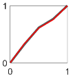
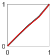
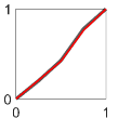
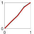
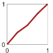
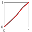
(c)		(d)		(e)

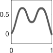
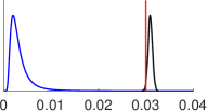
Figure 4: Illustration of the proposed approach based on simulated data. (a) A subset of simulated functions $f_{1:100}$. The target posterior distribution of template function and phase components given $f_{1:100}$, generated via recursive updates of samples from the posterior distribution given $f_{1:30}$, is illustrated using weighted samples (black with transparency reflecting the magnitude of the weights). (b) Weighted samples of (a subset of) phase components are shown in black and the ground truth components are in red. (c) Weighted samples of template function are shown in black, and (d) shows their corresponding SRVFs with the SRVF of the ground truth template function in red. (e) The unnormalized marginal posterior distribution of the error variance $\sigma^{2}$ given $f_{1:100}$ is visualized through a kernel density estimate (black). The prior distribution of $\sigma^{2}$ and the ground truth value of $\sigma^{2}$ are shown in blue and red, respectively.

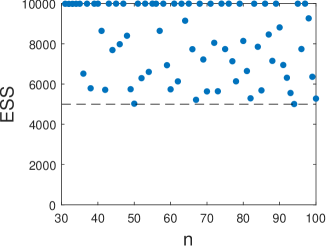
Figure 5: Effective sample size of weighted samples in Simulated Example 1 for a sequence of posterior distributions, $\pi(\cdot\mid f_{1:n}),\ n=31,\ldots,100$. The number of given functions $n$ is on the $x$-axis and the ESS of the weighted samples drawn from the corresponding posterior distributions is on the $y$-axis.

We first obtain a sample of size $10,000$ from the posterior distribution of the parameters given the first 30 functions, $f_{1:30}$, via MCMC-based batch learning. We take this MCMC sample as a set of equally weighted particle inputs to the subsequent SMC update. One function at a time is added to the data $f_{1:30}$, and the weighted samples are updated recursively using the SMC Algorithm 1; we employ parallel computing with 12 workers. The resulting weighted samples are shown in Figure 4. For template function and phase components, we use the (scaled) weight of each particle to adjust its transparency level to visualize posterior uncertainty. The SRVF of the ground truth template function and the ground truth phase components are superimposed in red, and lie within the corresponding $95\%$ pointwise marginal credible intervals in all cases. It is clear from Figure 4 that the proposed method is very effective at recovering the underlying template and phase components. We monitor the effective sample size to check for particle degeneracy. Figure 5 shows that the ESS of weighted samples at each update remains relatively large as we add more functions to the data.

Method	Template Function (c)		Phase Components ($\textbf{d}_{1:100}$)
	Posterior Mean	Posterior Mode	Posterior Mean	Posterior Mode
SMC	0.1317	0.1147	0.0080	0.0061
MCMC	0.2153	0.1890	0.0097	0.0083

Table 1: Comparison of estimation accuracy, based on Euclidean distances between the ground truth parameters and their posterior estimates, based on the proposed sequential approach (SMC) and MCMC-based batch learning. Best performance is given in bold.

For comparison, we implement MCMC-based batch learning given the full dataset $f_{1:100}$, which includes both Gibbs steps and adaptive Metropolis-Hastings updates [26, 30]. We use a total of $50,000$ MCMC iterations, with a burn-in period of $40,000$. We compare estimation results based on the proposed sequential Bayesian learning approach and the MCMC-based batch learning method. For the template function, we compute the Euclidean norm of the difference between the ground truth basis coefficients and the posterior mean and mode estimates produced by the two methods. For the phase components, we compute the sum of Euclidean distances between the ground truth phase increments and the posterior mean and mode estimates produced by the two methods. The results are reported in Table 1. The proposed sequential approach outperforms the MCMC-based batch learning approach for estimation in all scenarios. While not presented in this table, similar results hold for all intermediate posterior distributions in the sequence.

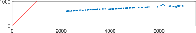
Figure 6: Comparison of computation time (in seconds) to generate $10,000$ samples from the sequence of posterior distributions, $\pi(\cdot\mid f_{1:31}),\ \pi(\cdot\mid f_{1:32}),\ldots,\ \pi(\cdot\mid f_{1:100})$. The MCMC-based batch learning time is on the $x$-axis with computation time for the proposed sequential approach on the $y$-axis. The proposed approach is initialized by generating $10,000$ posterior samples from $\pi(\cdot\mid f_{1:30})$ using MCMC. The red $45^{\circ}$ line acts as a reference.

We further compare the computational efficiency of the two methods. For the proposed sequential approach, we start with posterior samples given the data $f_{1:31}$, recursively add one function to the data at a time, and update the weighted samples using Algorithm 1. We do this for the full sequence of posterior distributions until all of the data, $f_{1:100}$, is used. For the MCMC-based batch learning approach, we draw samples from each posterior distribution in the sequence by re-running the full algorithm each time. As before, we use a total of $50,000$ MCMC iterations, with a burn-in period of $40,000$. Figure 6 compares the computation time (in seconds) needed to obtain a sample of size $10,000$ from each posterior distribution in the sequence, by conditioning on data $f_{1:n},\ n=31,\ldots,100$ corresponding to each blue point in the plot, using the two methods: MCMC computation time is shown on the $x$-axis and the proposed SMC-based computation time is shown on the $y$-axis; the red $45^{\circ}$ line serves as a reference. The computation times of the two methods appear linearly related as the sample size of the data increases. However, when compared to the red reference, it is clear that the proposed SMC-based approach for registration of functional data is much more computationally efficient than MCMC-based batch learning, especially when the sample size of the data is large. This significant gain in computational efficiency is expected due to the sequential nature of the proposed method.

For both MCMC-based batch learning and the proposed SMC method, the marginal posterior distribution of the error variance tends to overestimate the ground truth error variance across the sequence of target posterior distributions. This is due to the presence of temporal dependence in the error structure. To account for such temporal dependence, we may adopt a more complicated error structure; this aspect is left as future work. Even without the more complex error structure in the likelihood, the proposed approach is very effective in estimating the underlying template function and the phase components.

5.2 Simulated example 2

(a)
(b)
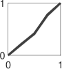
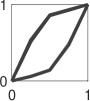
(c)
			(d)

Figure 7: Illustration of the proposed approach based on simulated data leading to a multimodal target posterior. (a) Simulated functions $f_{1:7}$. Weighted samples (black with transparency reflecting the magnitude of the weights) from the target posterior distribution of the (b) phase components and (d) template function, given $f_{1:7}$, generated via recursive updates of samples from the posterior distribution given $f_{1:3}$. (c) Functions $f_{1:7}$ after applying the corresponding posterior samples of the phase components, to visualize the registration of each function with respect to the template posterior samples.

Next, we assess the performance of the proposed sequential approach for registration of functional data when one of the target posterior densities is multimodal. For this, we simulate seven functions; the first six have two peaks while the seventh has only one. As in Simulated Example 1, we apply random phase components, generated as piecewise linear functions with Dirichlet increments at $M_{\gamma}=5$ equally spaced locations with concentration parameter $\kappa=40$. The full data $f_{1:7}$ is shown in Figure 7(a). All prior hyperparameters for the Bayesian registration model are the same as those in Simulated Example 1, except for $\alpha_{\sigma}=40$.

We initialize Algorithm 1 using samples from the posterior distribution given $f_{1:3}$, via MCMC-based batch learning. We then add functions $f_{4:7}$ to the data, one function at a time, and update the weighted samples sequentially to target the posteriors $\pi(\cdot\mid f_{1:4}),\ldots,\pi(\cdot\mid f_{1:7})$. Once all of the functions have been included as part of the data, we expect the template components of most of the particles to have two peaks, since most of the data has this form. Since phase is relative with respect to the template, the samples corresponding to the phase component for function $f_{7}$ should cluster into two distinct groups: ones that register the single peak in function $f_{7}$ to the left peak of the template and ones that register it to the right peak of the template. Thus, we expect the marginal posterior of the phase component for function $f_{7}$ to be bimodal.

The results of this simulation are presented in Figure 7. As seen in panel (d), indeed, the template components of the particles appear to have two peaks. The phase components of the particles, shown in panel (b), corresponding to functions $f_{1:6}$ do not appear to indicate multimodality in the marginal posterior. However, the phase components of the particles corresponding to function $f_{7}$ clearly fall into two distinct groups. The first group, which falls above the identity, registers the peak in $f_{7}$ to the first peak in the template function. The second group, which falls below the identity, registers the peak in $f_{7}$ to the second peak of the template function. This is also evident in Figure 7(c). Thus, the proposed sequential approach is able to approximate the bimodal target posterior density well. On the other hand, standard MCMC-based batch learning algorithms often fail to explore multimodal posterior distributions, and must resort to more advanced techniques such as parallel tempering to overcome this issue.

5.3 Real data analysis 1: drought intensity measurements near Kaweah River in California

(a)
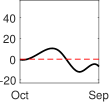
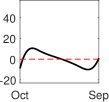
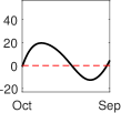
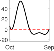
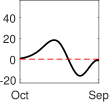
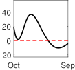
(b)
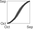
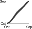
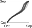
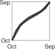
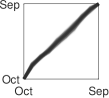
(c)		(d)		(e)

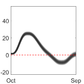
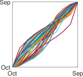
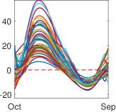
Figure 8: Sequential Bayesian registration of SPEI functions representing drought intensity. (a) Trajectories of recent annual drought intensity near Kaweah River in California from 2014 to 2019 (hydrological year). (b) Weighted posterior draws of the relative phase components for the functions displayed in (a), and (c) weighted samples of the template function of the target posterior distribution given SPEI functions from 1970 to 2019 where transparency reflects the magnitude of the weight of each sample. (d) Marginal posterior means of the relative phase components for the SPEI functions from 1970 to 2019. (e) Registration of the 50 functions via the estimated marginal posterior means of the relative phase components shown in (d). The black dashed lines in (a), (c) and (e) represent the threshold at which a drought period begins and ends.

The proposed method can be effective in analyzing trajectories of annual measurements related to the climate, as they are often monitored sequentially. One annual measurement that exhibits a common template across years, along with phase variation, is drought intensity. We consider sequential Bayesian registration of trajectories of annual drought intensity near Kaweah River in California. Statistical analysis of drought helps inform future management and allocation of water, and preparation for severe drought seasons. Importantly, drought intensity in California has been of great interest to address the state’s drought risk management and limited access to water; Californians rely on the West and East Sierra Nevadan water resources due to intense drought in other areas of the state [36]. A lot of attention in the literature has been devoted to developing new models for annual drought intensity, with an overarching goal of predicting future drought. However, this task is challenging due to the time-varying and confounded nature of the variation in drought intensity magnitude and relative phase due to meteorologic and anthropogenic changes in the climate [37, 38]. In particular, annual drought intensity measurements often exhibit a time lag as well as seasonal variation. Thus, interest not only lies in the magnitude of drought intensity, but also in the times at which drought periods begin and end during a particular year; this feature of drought intensity is captured through phase and can improve our understanding of variation in the drought lead time [39].

In this study, we use scaled Standardised Precipitation-Evapotranspiration Index (SPEI) measurements for the Kaweah River in California throughout the years 1970 to 2019, obtained from the PRISM dataset, to represent drought intensity [40, 41]. To generate functional data of annual drought intensity, we apply basis spline regression to monthly (scaled) SPEIs. We refer to this data as annual SPEI functions (hydrological year; Oct 1 to Sep 30), denoted by $f_{1:50}$, and display a subset of it in Figure 8(a).

We model the template function as a linear combination of B-spline bases with unknown coefficients, and specify the following prior hyperparameters for the template and phase components: $B=10,\ \Sigma_{c}=20I_{B},\ \kappa=5,\ \alpha_{\sigma}=4,\ \beta_{\sigma}=0.01$, and a uniform partition of size $M_{\gamma}=10$. We first draw $10,000$ samples from the posterior distribution given $f_{1:30}$ using MCMC-based batch learning; we use a burn-in period of $40,000$. The rest of the SPEI functions $f_{31:50}$ are added to the data sequentially, and the initial samples are updated recursively via Algorithm 1.

Features of the target posterior density, $\pi(\cdot|f_{1:50})$, are visualized in Figure 8. Drought begins when SPEI values become negative and ends when they become positive; this threshold is highlighted by the black dashed line in panels (a), (c) and (e). Panel (c) shows weighted samples of the template function (the transparency of each sample reflects the magnitude of the corresponding weight), given the annual SPEI functions $f_{1:50}$ of which a subset is displayed in panel (a). It appears that drought in the Kaweah River generally starts approximately in mid-April and ends in late September. However, there appears to be significant variation in the time at which the template samples cross the drought onset threshold. Panel (c) visualizes weighted samples of phase components for the SPEI functions $f_{45:50}$ and panel (d) illustrates annual phase variability of the SPEI functions $f_{1:50}$ via the marginal posterior means of the relative phase components. There appears to be significant phase variation throughout each year in this dataset. It appears that there is more phase variation from October to April than from May until the end of the hydrological year. Such estimates of the relative phase components aid in the analysis of variation in drought duration as well as the timing of drought onset across years.

Figure 8(e) shows the SPEI functions $f_{1:50}$, but after registration via the estimated marginal posterior mean phase components. In each calendar year, drought intensity in the Kaweah River is the smallest in early January, corresponding to the large peaks in the registered SPEI functions. On the other hand, drought intensity appears the largest in mid-July, corresponding to the lowest valley in the registered SPEI functions. It is evident that amplitude variability in the SPEI functions is much larger during the winter season as compared to the drought season in the summer. In particular, the magnitude of most severe drought (minimum values in the SPEI functions) is similar across all years.

5.4 Real data analysis 2: annual sea surface salinity near Null Island

Next, we consider trajectories of annual sea surface salinity magnitude near Null Island. Salinity is an important feature in global climate change as it regulates the movement of currents and heat carried within currents based on water density [42]. As water evaporation and precipitation changes over time, the magnitude of sea surface salinity fluctuates annually according to seasonal variability. Estimation of the relative phase components of annual measurements of salinity is thus an important statistical task, as these can be subsequently used for prediction of future phase variation and estimation of the lag between fluctuations of salinity and precipitation; precipitation is a major factor that affects ocean salinity and their relationship is of great interest.

(a)
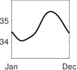
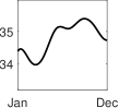
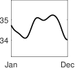
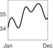
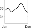
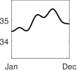
(b)
(c)		(d)		(e)

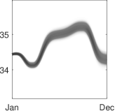
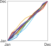
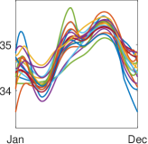
Figure 9: Sequential Bayesian registration of sea surface salinity functions. (a) Trajectories of annual sea surface salinity near Null Island from 2012 to 2017. (b) Weighted samples of the relative phase components for the functions displayed in (a), and (c) weighted samples of the template function of the target posterior distribution given SSS functions from 2000 to 2017 where transparency reflects the magnitude of the weight of each sample. (d) Marginal posterior means of the relative phase components for the SSS functions from 2000 to 2017. (e) Registration of the 18 SSS functions via the estimated marginal posterior means of the relative phase components shown in (d).

We apply the proposed sequential registration method to annual sea surface salinity (SSS) functions collected near Null Island. We use the EN4 data from 2000 to 2017, and smooth each set of annual SSS measurements using ten spline basis functions [43, 44]. This results in annual SSS functional data, $f_{1:18}$, which is displayed in Figure 9(a). The SSS functions share a common pattern of local extrema with clear phase variation. In a previous study, Bingham et al. approximated seasonal variability across years through a one-dimensional measurement of phase, corresponding to the time at which maximum SSS magnitude is observed [45]. This is akin to landmark-based registration of the functions, with the point of maximum SSS magnitude on each function serving as a single landmark. This approach is effective at registering the landmarks, but it fails to register other prominent features of the functions. Thus, to estimate more flexible and informative relative phase components of the SSS functional data, we apply the proposed sequential Baysian registration approach.

The common template is modeled as a linear combination of B-spline bases with unknown coefficients. Prior hyperparameters for the template and phase components are: $B=10,\ \Sigma_{q}=20I_{B},\ \kappa=5,\ \alpha_{\sigma}=4,\ \beta_{\sigma}=0.01$, and a uniform partition of size $M_{\gamma}=10$. We first draw $10,000$ samples from the posterior distribution given $f_{1:10}$ using MCMC-based batch learning; we use a burn-in period of $40,000$. The rest of the SSS functions, $f_{11:18}$, are added to the data sequentially, and the initial samples are updated recursively via Algorithm 1.

Features of the target posterior density, $\pi(\cdot\mid f_{1:18})$, are visualized in Figure 9. In panel (b), we show weighted samples of (a subset of) the phase components (the transparency of each sample reflects the magnitude of the corresponding weight), given the annual SSS functions $f_{1:18}$, with a subset of the functions displayed in panel (a). The samples of the template function clearly capture the prominent features of the SSS functional data (panel (c)). In particular, the template reflects relatively high SSS from May to November with a maximum around October, while the lowest SSS occurs around March. The marginal posterior means of the phase components of the SSS functional data are shown in panel (d). It appears that there is more phase variation from January to May than from June until the end of the year. Further, the relative phase components of SSS functions for years 2000, 2005 and 2017 (yellow, dark blue and light blue functions in panel (d)) are much further from the identity than the relative phase components of SSS functions for the other years. Finally, panel (e) displays the SSS functions from 2000 to 2017, but after registration via the estimated marginal posterior mean phase components. The SSS functions appear to be horizontally synchronized after registration as desired.

5.5 Real data analysis 3: PQRST complexes segmented from long electrocardiogram signal

(a)
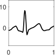
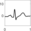
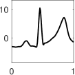
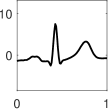
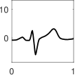
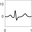
(b)
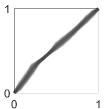
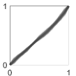
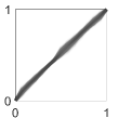
(c)		(d)		(e)

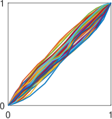
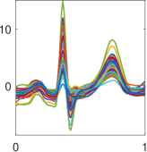
Figure 10: Sequential Bayesian registration of PQRST complexes extracted from an ECG signal. (a) A subset of 50 PQRST complexes. (b) Weighted samples of the phase components for the functions in (a), and (c) weighted samples of the template function where transparency reflects the magnitude of the weight of each sample. (d) Marginal posterior means of the relative phase components for the 50 functions. (e) Registration of the functional data via the estimated marginal posterior means of the relative phase components shown in (d).

The electrocardiogram (ECG) is routinely used to assess heart function and diagnose various medical conditions such as myocardial infarction. The data recorded via ECG is a long ECG signal composed of a periodic sequence of a pattern known as the PQRST complex: the P wave corresponds to the first small peak, the QRS wave is composed of a sharp valley followed by a sharp peak followed by another sharp valley, and the T wave represents the last high peak. Prior to statistical analysis, it is beneficial to first segment the long ECG signal into its PQRST complexes [46]. Our focus here is not on the segmentation problem, but rather on registration of PQRST complexes as the long ECG signal is recorded and segmented sequentially. While there is natural variability among the PQRST complexes along an ECG signal, abnormalities in estimates of the underlying template function and variation in timing of the PQRST patterns with respect to that template (phase components) are beneficial for the aforementioned diagnostic purposes. For example, the duration of the QT interval is useful in drug development and approval [47].

We consider 50 PQRST complexes, denoted by $f_{1:50}$, segmented form a long ECG signal [46]; six functions among them are displayed in Figure 10(a). We first obtain $10,000$ posterior samples via MCMC-based batch learning based on the data $f_{1:50}$. We use the same MCMC settings (total iteration and burn-in period) as in the previous real data examples. The template function is modeled as a linear combination of $13$ B-spline basis functions with $\Sigma_{c}=20I_{B}$. The concentration parameter defining the increments of the phase components is $\kappa=5$ and the size of the uniform partition is $M_{\gamma}=15$. Finally, the hyperparameters for the error variance are $\alpha_{\sigma}=10$ and $\beta_{\sigma}=0.01$.

Estimation results, based on the last posterior distribution in the sequence, $\pi(\cdot\mid f_{1:50})$, are illustrated in Figure 10. Panel (b) shows the weighted samples of the phase components for the functions in (a), and panel (c) visualizes the weighted samples of the template function with transparency reflecting the magnitude of the weights. The estimated template function contains all features of the PQRST complex and is representative of the structure in the given data. The marginal posterior means of the phase components are shown in panel (d). In general, they capture the relative acceleration or delay of the corresponding PQRST complex with respect to the template. The posterior means of the phase components have relatively similar variation across the domain compared to the real data studies on environmental monitoring. The registered data, obtained by applying the posterior mean phase components in (d) to the corresponding PQRST complexes, is shown in panel (e). The proposed method achieves very good horizontal synchronization of all features of the PQRST complexes.

6 Discussion and future work

We propose a novel sequential Bayesian registration method for functional data that addresses two common challenges: confounded variability across functions, and availability of an increasing number of functional observations over time. In particular, we propose a Bayesian registration model and a custom SMC algorithm to update inference when a new function is observed, exploiting a deterministic kernel for introducing new state variables and an approximate weight updating approach for MH kernels without a closed form. We illustrate the performance of the proposed approach through several simulation studies and real data examples. We show that the proposed sequential learning algorithm is computationally more efficient, and more accurate in terms of posterior estimates, compared to the batch MCMC algorithm. It also behaves desirably for exploring multimodal posterior distributions, which often pose a challenge for many MCMC techniques. Application of this framework to real data studies improves our understanding of the underlying structure of the data, and provides quantitative evidence to study associated research problems.

An important consideration is that the proposed method leads to approximate posterior inference due to the need to circumvent computation of the MH and Gibbs kernels in the SMC algorithm. The quality of the approximation depends on the following assumptions. First, marginals of adjacent posterior distributions must be similar. In general, this holds when a new function is assimilated with a relatively large number of functions that are already registered. If the number of previously registered functions is small, and a function with a very different shape arrives, the difference in the marginal posteriors may lead to non-representative weights. In such cases, we suggest adding annealing steps between adjacent target distributions. With this adjustment, the proposed algorithm is robust to outlying functions that have potentially different shape relative to other functions already in the sample.

Particle degeneracy often arises in SMC sampling for a sequence of distributions with increasing state space dimension, and can lead to unreliable posterior estimates. We partly resolve this issue by initializing new components of each particle such that the updated particles lie in a region of high posterior probability. In the current inferential setting, where phase components are added to the state space as new data arrives, this initialization can be performed for each particle by registering the new functional observation to that particle’s template using a computationally efficient optimization-based technique. Furthermore, we monitor the effective sample size (ESS) throughout the algorithm, because small values of ESS can indicate evidence of particle degeneracy. In the increasing state space dimension setting, degeneracy may be remedied by duplicating existing particles, thereby increasing the number of weighted samples. This was not necessary in our studies, as the ESS was large and no significant decrease in ESS was observed as we added more functions to the data.

The proposed Bayesian registration model may be modified depending on the application of interest. The key assumption that makes the model computationally tractable is that phase components are piecewise linear functions with Dirichlet increments. This reduces the state space dimension relative to similar models in the literature and enables faster posterior inference. Another consideration is that, for the sake of isometry and simple derivations, we build the Bayesian hierarchical model on the SRVF space. This limits our model to functions for which derivatives exist almost everywhere. The proposed method is therefore applicable to various real data studies where interest lies in smooth evolutions of a variable.

In future work, we will incorporate functional correlation over time in the model. This is a reasonable assumption for applications such as climate monitoring, when functional variability is dependent between observations. This includes extending the proposed model to account for functional autocorrelation using a functional time series model [48, 49].

References

- [1] F. Ferraty and P. Vieu. Nonparametric Functional Data Analysis: Theory and Practice. Springer Series in Statistics. Springer New York, 2006.
- [2] H. Lajos and P. Kokoszka. Inference for Functional Data with Applications. Springer Series in Statistics. Springer New York, 2012.
- [3] J. O. Ramsay and C. J. Dalzell. Some tools for functional data analysis. Journal of the Royal Statistical Society, Series B, 53(3):539–561, 1991.
- [4] J. Ramsay and B. W. Silverman. Functional Data Analysis. Springer Series in Statistics. New York: Springer, 2005.
- [5] S. CH Hoi, D. Sahoo, J. Lu, and P. Zhao. Online learning: A comprehensive survey. arXiv preprint arXiv:1802.02871, 2018.
- [6] C. Andrieu, N. Freitas, and A. Doucet. Sequential MCMC for Bayesian model selection. pages 130 – 134, 02 1999.
- [7] G. Storvik. Particle filters for state space models with the presence of static parameters. Signal Processing, IEEE Transactions on, 50:281 – 289, 03 2002.
- [8] H. Lopes and R. Tsay. Particle filters and Bayesian inference in financial econometrics. Journal of Forecasting, 30:168–209, 01 2011.
- [9] N. Schweizer. Non-asymptotic error bounds for sequential MCMC methods in multimodal settings, 2012.
- [10] D. Paulin, A. Jasra, and A. H. Thiery. Error bounds for sequential Monte Carlo samplers for multimodal distributions. Bernoulli, 2019.
- [11] C. Dai, J. Heng, P. E. Jacob, and N. Whiteley. An invitation to sequential Monte Carlo samplers. arXiv: Computation, 2020.
- [12] W. R. Gilks and C. Berzuini. Following a moving target—Monte Carlo inference for dynamic Bayesian models. Journal of the Royal Statistical Society - Series B, 63(1):127–146, 2001.
- [13] N. Chopin. A sequential particle filter method for static models. Biometrika, 89(3):539–552, 08 2002.
- [14] P. Del Moral, A. Doucet, and A. Jasra. Sequential Monte Carlo samplers. Journal of the Royal Statistical Society, Series B, 68:411–436, 02 2006.
- [15] N. Kantas, A. Beskos, and A. Jasra. Sequential Monte Carlo methods for high-dimensional inverse problems: A case study for the Navier–Stokes equations. SIAM/ASA Journal on Uncertainty Quantification, 2, 07 2013.
- [16] A. Beskos, A. Jasra, E. A. Muzaffer, and A. M. Stuart. Sequential Monte Carlo methods for Bayesian elliptic inverse problems. Statistics and Computing, 25:727–737, 2015.
- [17] J. Liu and M. A. West. Combined parameter and state estimation in simulation-based filtering. In Sequential Monte Carlo Methods in Practice, 2001.
- [18] J. Ramsay and X. Li. Curve registration. Journal of the Royal Statistical Society, Series B, 60:351 – 363, 01 1998.
- [19] J. S. Marron, J. O. Ramsay, L. M. Sangalli, and A. Srivastava. Functional Data Analysis of Amplitude and Phase Variation. Statistical Science, 30(4):468 – 484, 2015.
- [20] R. Tang and H. Müller. Pairwise curve synchronization for functional data. Biometrika, 95(4):875–889, 2008.
- [21] A. Srivastava, W. Wu, S. Kurtek, E. Klassen, and J. S. Marron. Registration of functional data using Fisher-Rao metric. arXiv: Statistics Theory, 2011.
- [22] A. Kneip, X. Li, K. B. MacGibbon, and J. O. Ramsay. Curve registration by local regression. The Canadian Journal of Statistics / La Revue Canadienne de Statistique, 28(1):19–29, 2000.
- [23] S. I. Amari. Differential Geometric Methods in Statistics. Lecture Notes in Statistics, Vol. 28. Springer, 1985.
- [24] P. W. Vos and R. E. Kass. Geometrical Foundations of Asymptotic Inference. Wiley-Interscience, 1997.
- [25] D. Telesca and L. Y. T Inoue. Bayesian hierarchical curve registration. Journal of the American Statistical Association, 103(481):328–339, 2008.
- [26] Y. Lu, R. Herbei, and S. Kurtek. Bayesian registration of functions with a Gaussian process prior. Journal of Computational and Graphical Statistics, 26(4):894–904, 2017.
- [27] W. Z. Horton, G. L. Page, C. S. Reese, L. K. Lepley, and M. White. Template priors in Bayesian curve registration. Technometrics, 63(4):487–499, 2021.
- [28] W. Cheng, I. Dryden, and X. Huang. Bayesian registration of functions and curves. Bayesian Analysis, 11(2):447–475, 2016.
- [29] K. Bharath and S. Kurtek. Distribution on warp maps for alignment of open and closed curves. Journal of the American Statistical Association, 115(531):1378–1392, 2020.
- [30] J. Matuk, K. Bharath, O. Chkrebtii, and S. Kurtek. Bayesian framework for simultaneous registration and estimation of noisy, sparse, and fragmented functional data. Journal of the American Statistical Association, 0(0):1–17, 2021.
- [31] J. S. Liu and R. Chen. Sequential Monte Carlo methods for dynamic systems. Journal of the American Statistical Association, 93(443):1032–1044, 1998.
- [32] D. P. Bertsekas. Dynamic Programming and Optimal Control. Athena Scientific, 2nd edition, 2000.
- [33] A. Srivastava and E. P. Klassen. Functional and Shape Data Analysis. Springer Series in Statistics. Springer New York, 2016.
- [34] M. A. West. Approximating posterior distributions by mixtures. Journal of the Royal Statistical Society, Series B, 55:409–422, 1993.
- [35] N. J. Gordon, D. J. Salmond, and A. F. M. Smith. Novel approach to nonlinear/non-Gaussian Bayesian state estimation. IEEE Proceedings F (Radar and Signal Processing), 140:107–113(6), April 1993.
- [36] M. E. Mann and P. H. Gleick. Climate change and California drought in the 21st century. Proceedings of the National Academy of Sciences, 112(13):3858–3859, 2015.
- [37] N. S. Diffenbaugh, D. L. Swain, and D. Touma. Anthropogenic warming has increased drought risk in California. Proceedings of the National Academy of Sciences, 112(13):3931–3936, 2015.
- [38] B. Son, J. Im, S. Park, and J. Lee. Satellite-based drought forecasting: Research trends, challenges, and future directions. Korean Journal of Remote Sensing, 37:815–831, 08 2021.
- [39] A. Dikshit, B. Pradhan, and A. M. Alamri. Long lead time drought forecasting using lagged climate variables and a stacked long short-term memory model. Science of The Total Environment, 755:142638, 2021.
- [40] Y. Kim and N. E. Grulke. 80-year meteorological record and drought indices for Sequoia National Park and Sequoia National Monument, CA. Forest Service Research Data Archive, 2022.
- [41] S. M. Vicente-Serrano, S. Beguería, and J. I. López-Moreno. A multiscalar drought index sensitive to global warming: The standardized precipitation evapotranspiration index. Journal of Climate, 23(7):1696 – 1718, 2010.
- [42] P. J. Durack. Ocean salinity and the global water cycle. Oceanography, 28(1):20–31, 2015.
- [43] British Crown Copyright Met Office. En.4.2.2 data, 2021.
- [44] S. A. Good, M. J. Martin, and N. A. Rayner. EN4: Quality controlled ocean temperature and salinity profiles and monthly objective analyses with uncertainty estimates. Journal of Geophysical Research: Oceans, 118(12):6704–6716, 2013.
- [45] F. M. Bingham, S. Brodnitz, and L. Yu. Sea surface salinity seasonal variability in the tropics from satellites, gridded in situ products and mooring observations. Remote Sensing, 13(1), 2021.
- [46] S. Kurtek, W. Wu, G. E. Christensen, and A. Srivastava. Segmentation, alignment and statistical analysis of biosignals with application to disease classification. Journal of Applied Statistics, 40(6):1270–1288, 2013.
- [47] Y. Zhou and N. Sedransk. Functional data analytic approach of modeling ECG T-wave shape to measure cardiovascular behavior. The Annals of Applied Statistics, 3(4):1382 – 1402, 2009.
- [48] D. Bosq. Linear Processes in Function Spaces: Theory and Applications. Lecture Notes in Statistics. Springer New York, 2000.
- [49] P. Kokoszka. Dependent functional data. ISRN Probability and Statistics, 2012, 01 2012.