Bearing-Based Formation Control with Optimal Motion Trajectory

Abstract

Bearing-based distributed formation control is attractive because it can be implemented using vision-based measurements to achieve a desired formation. Gradient-descent-based controllers using bearing measurements have been shown to have many beneficial characteristics, such as global convergence, applicability to different graph topologies and workspaces of arbitrary dimension, and some flexibility in the choice of the cost. In practice, however, such controllers typically yield convoluted paths from their initial location to the final position in the formation. In this paper we propose a novel procedure to optimize gradient-descent-based bearing-based formation controllers to obtain shorter paths. Our approach is based on the parameterization of the cost function and, by extension, of the controller. We form and solve a nonlinear optimization problem with the sum of path lengths of the agent trajectories as the objective and subject to the original equilibria and global convergence conditions for formation control. Our simulation shows that the parameters can be optimized from a very small number of training samples (1 to 7) to straighten the trajectory by around 16% for a large number of random initial conditions for bearing-only formation. However, in the absence of any range information, the scale of the formation is not fixed and this optimization may lead to an undesired compression of the formation size. Including range measurements avoids this issue and leads to further trajectories straightening by 66%.

I Introduction

The goal of multi-agent formation control is to use distributed control to drive a number of agents to a desired geometric pattern. The advantages of such a system include the possibility of controlling a large network by a single operator, and the robustness of the system to failures of a single agent. As a results, formation control approaches have been widely applied to a variety of applications including surveillance, exploration, and transportation [1, 2, 3].

Compared to the extensively studied distance-based formation control [4], bearing-based formation methods are appealing since relative bearing measurements are easy to obtain from an on-board camera and they are often more reliable than distance measurements, especially when the agents are relatively far away.

Review of prior work. While there has been significant work in formation control, we limit ourselves to the progress in bearing-based formation control. The initial work of distributed bearing-based formation control traces back at least two decades [5, 6, 7]. However, the distance corresponding to each bearing measurement is required by the control law. The control method proposed in [8] provided fast and straight trajectories using zero or one distance measurement, but it relied either on special graph topologies based on two leader agents, or on distributed estimators that virtually realize the measurements of such topologies. A more recent method was based on the gradient control law that does not depend on the distances, with the stability analysis relying on the state of the entire network evolving on a sphere [9, 10].

Following the above work, another gradient-based control law that requires only relative bearing measurements, but can also handle optional distance measurements was proposed in [11] (which extended an earlier work on the visual homing method from [12]). The control is based on the gradient of a Lyapunov function; global convergence is guaranteed by imposing constraints on this function. Advantages of this method include the fact that it can cover arbitrary numbers of agents, graph topologies and workspace dimensions. Several works have extended [11] to more settings including second order dynamics [13], double integrator and unicycle dynamics [14, 15], directed acyclic graphs and directed cycle graphs [16]. All these works are based on a particular choice of the Lyapunov function defining the gradient-based controller, despite the fact that the stability conditions in the original work [11] allow some flexibility in this regard.

Other prior work has established a solid theoretical footing for the approach, establishing the concept of bearing rigidity theory [10] and developing bearing based control laws [7, 9, 11, 17]. However, a notable gap in the previous literature is that, while ensuring global convergence, there is no attempt to characterize, let alone optimize, the length and smoothness of the trajectories of the multi-agent system during their transitory phase. Typical trajectories of this controller are shown in the examples of Fig. 1a, 1b.

A natural objective, then, is to optimize the path length of the agents, ideally reaching straight lines (i.e, the shortest possible path). Such a problem is not straightforward since each agent has very limited information about the global state of the network: it only observes its neighbors, moreover, it may observe only the directions, which is a nonlinear function of the state. As such, it is not trivial to find a controller that guides the agents along the shortest linear paths. In this paper, we focus on finding controllers that minimize the agents’ path lenght for gradient-based bearing-based formation control with optional range measurements.

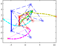
(a)

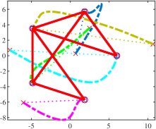
(b)

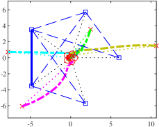
(c)

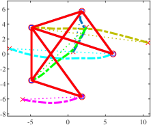
(d)

Figure 1: (a)(c): bearing-only 5-agent sytem where $E_{d}=\emptyset$, (b)(d): bearing-based 5-agent system where $E_{b}=E_{d}$. Agents’ given desired formation are moving via thick dashed lines from initial to desired locations. First row is before the optimization and second row is after.

Paper contributions. Our key contributions are:

• We modify the convergence proof in [11] to relax the conditions on the control cost for bearing-only formation and thereby expand the class of functions that can be used in the controller that guarantee global convergence.

• While maintaining global convergence, we formulate a constrained nonlinear optimization problem to find parameters for the Lyapunov function that leads to straighter trajectories.

• We apply the optimization to bearing-based controllers and highlight an undesirable collapse effect that appears when using minimum path length as the objective. We further show that by including any number of range measurements in the controller, this effect can be avoided.

To evaluate the optimization results, we use two performance metrics: percentage of improvement in trajectory length relative to the original path, and percentage of improvement in trajectory length difference relative to an ideal straight-line path. Through simulations, we demonstrate that for these two metrics, our method improves the performance by approximately 8% and 16%, respectively, in a simulated 5-agent bearing-only network. Including additional range measurements leads to an improvement of approximately 11% and 66% respectively. We also show that even with a small number of training initial conditions, the improvements generalize to (1) a far larger number of testing initial conditions, (2) a different number of agents, and (3) various target formation shape.

II Preliminaries

We denote the dimension of the work-space with $n$. We assume that agents acquire bearing measurements in their own local reference frame, but that all the local reference frames are rotationally aligned (equivalently, the agents know their rotation with respect to a common global frame [18]), and all the quantities discussed are expressed in a common global inertial reference frame (e.g., by assuming the availability of a compass for each agent). The operator $\operatorname{stack}(v_{1},\dots,v_{m})=\operatorname{stack}(\{v_{i}\}_{i=1}^{m})$ returns the vector obtained by vertically stacking the arguments.

II-A Graph Theory

The interaction topology of a multi-agent system is modeled as a directed graph $\mathcal{G}=(\mathcal{V},\mathcal{E})$, where $\mathcal{V}$ denotes the set of nodes, $\mathcal{E}\subseteq\mathcal{V}\times\mathcal{V}$ denotes the edges of ordered pairs of the nodes, and the set of neighbors of $i\in\mathcal{V}$ is $\mathcal{N}_{i}:=\{j\in\mathcal{V}:(i,j)\in\mathcal{E}\}$. A graph is undirected if for every $(i,j)\in\mathcal{E}$, $(j,i)$ is also in $\mathcal{E}$. We assume all graphs are undirected (as it will be seen from the definitions in the following section, measurements for the edge $j\to i$ can be easily obtained from those for edge $i\to j$ via communication).

II-B Formations and Measurements

We represent the set of $N$ agents as $\mathcal{V}=\{1,\dots,N\}$ and the corresponding location of each agent as $\{x_{i}\}_{i\in\mathcal{V}}$. We define the range between nodes $i,j\in\mathcal{V}$ as

$$d_{ij}(x_{i},x_{j})=\lVert x_{j}-x_{i}\rVert,$$ (1)

where $\|\cdot\|$ denotes the Euclidean norm. The bearing direction is defined as

$$\beta_{ij}(x_{i},x_{j})=d_{ij}^{-1}(x_{j}-x_{i}).$$ (2)

A bearing-based formation is defined as $\mathcal{F}=(\mathcal{G},\mathbf{x})$ where

• $\mathbf{x}=\operatorname{stack}(\{x_{i}\}_{i\in\mathcal{V}})$ is the configuration of the formation that gives the location of each agent in $\mathbb{R}^{n}$.

• $\mathcal{G}=(\mathcal{V},\mathcal{E}_{b},\mathcal{E}_{d})$ is a graph in which $\mathcal{E}_{b}$ contains the set of pairs $(i,j)$ where agent $i$ can observe $\beta_{ij}$ and $\mathcal{E}_{d}$ contains the set of pairs that observe $d_{ij}$. We assume that $\mathcal{E}_{d}\subset\mathcal{E}_{b}$.

$\mathcal{F}$ is a bearing-only formation if $\mathcal{E}_{d}=\emptyset$. The complete set of bearings and ranges of a formation is denoted by the vector $\boldsymbol{\beta}=\operatorname{stack}(\{\beta_{ij}\}_{(i,j)\in\mathcal{E}_{b}})$, $\mathbf{d}=\operatorname{stack}(\{d_{ij}\}_{(i,j)\in\mathcal{E}_{d}})$. Two formations $(\mathcal{G},\mathbf{x})$ and $(\mathcal{G},\mathbf{x^{\prime}})$, are said to be

• equivalent if they yield the same measurements, $\boldsymbol{\beta}\!=\!\boldsymbol{\beta^{\prime}}$, $\mathbf{d}=\mathbf{d^{\prime}}$.

• congruent if they have the same shape and scale, $x_{i}^{\prime}=x_{i}+t$ with $t\in\mathbb{R}^{n}$ and for all $i\in\mathcal{V}$.

• similar if they have the same shape, $x_{i}^{\prime}=\gamma x_{i}+t,\gamma>0$, with $t\in\mathbb{R}^{n}$ and for all $i\in\mathcal{V}$.

A formation $(\mathcal{G},\mathbf{x})$ is rigid if every configuration equivalent to it is also similar (for bearing-only) or congruent (for bearing+range) to it. In this paper, we assume that all formations are rigid.

II-C Gradient-based Formation Control

We take a simple kinematic motion model,

$$\mathbf{\dot{x}}=\mathbf{u},$$ (3)

and follow the derivation of the distributed gradient-based controller from [11]. The control is defined as

$$\mathbf{u}=-\frac{\partial\varphi(\mathbf{x})}{\partial x},$$ (4)

where the cost function $\varphi$ for a bearing-only formation is

$$\varphi(\mathbf{x})=\varphi_{b}(\mathbf{x})=\sum\limits_{(i,j)\in\mathcal{E}_{b}}\varphi_{ij}^{b}(x_{i},x_{j}),$$ (5)

$$\varphi_{ij}^{b}(x_{i},x_{j})=d_{ij}f_{b}(c_{ij}),$$ (6)

$$c_{ij}(x_{i},x_{j})=\beta_{g,ij}^{T}\beta_{ij}=\cos(\angle(\beta_{g,ij},\beta_{ij})),$$ (7)

where $\angle(\cdot,\cdot)$ denotes the angle between two vectors, $c_{ij}$ is referred to as a bearing similarity between the current bearing $\beta_{ij}$ and desired bearing $\beta_{g,ij}$, and $f_{b}(c_{ij})$ as a bearing reshaping function. In Sec. III, we derive a set of conditions on the bearing reshaping function to ensure global stability of the control law to the desired formation that are less restrictive than those found in [11]. The cost function (5) is a summation over the edges $\mathcal{E}_{b}$, with each term being a monotonic function of the similarity between the current and desired bearing. The control law (4) for any specific agent $i\in\mathcal{V}$ can be written as

$$u_{i}=-\sum\limits_{j:(i,j)\in\mathcal{E}_{b}}g^{b}_{ij}(x_{i},x_{j}),$$ (8)

where $g^{b}_{ij}$ denotes the gradient of (6) and is given by the following (a detailed derivation can be found in [12]):

$$g_{ij}^{b}=-f_{b}(c_{ij})\beta_{ij}-f^{\prime}_{b}(c_{ij})(I_{n}-\beta_{ij}\beta_{ij}^{T})\beta_{g,ij},$$ (9)

where $I_{n}\in\mathbb{R}^{n\times n}$ denotes an identity matrix, and $f^{\prime}_{b}(c_{ij})$ is the derivative of $f_{b}$ evaluated at $c_{ij}$. Note that although the unmeasured distance for each edge appears in the cost function, it does not appear in the bearing-only control law.

The bearing-based controller adds the range measurements to the cost function, yielding

$$\varphi(\mathbf{x})=\beta_{b}\sum\limits_{(i,j)\in\mathcal{E}_{b}}\varphi_{ij}^{b}(x_{i},x_{j})+\beta_{d}\sum\limits_{(i,j)\in\mathcal{E}_{d}}\varphi_{ij}^{d}(x_{i},x_{j}),$$ (10)

$$\varphi_{ij}^{d}(x_{i},x_{j})=f_{d}(q_{ij}),$$ (11)

$$q_{ij}(x_{i},x_{j})=d_{ij}c_{ij}-d_{g,ij},$$ (12)

where $q_{ij}$ is the range similarity between the current and desired range. The conditions on the range reshaping function $f_{d}(q_{ij})$ to ensure global convergence of the agents to the desired formation using the cost (10) are: (1) $f_{d}(q)>0$, $f_{d}(0)=0$, (2) $\text{sign}(f^{\prime}_{d}(q))=\text{sign}(q)$, (3) $f^{\prime\prime}_{d}(0)>0$ (see, e.g. [11]).

Remark 1

At the point where the controller is undefined (i.e. when $x_{i}=x_{j}$), the edge cost (6) becomes $0$ by continuity and one of the subgradient is $\mathbf{0}_{2n}$.

III Conditions for Bearing-only Global Convergence

We focus primarily on the bearing-only approach and provide the first contribution of the paper, namely a less restrictive set of constraints on the bearing reshaping function relative to those of [11] that ensure global convergence. First, we want to ensure that the gradient-based bearing-only controller converges to equilibria where the configuration is similar (in the sense defined in Sec. II-B) to the desired one. This implies that every minimum of $\varphi(\cdot)$ should be a global minimum (i.e., there are no spurious local minima). Following the reasoning of [11], such a condition can be achieved by requiring certain properties on the individual reshaping function $f_{b}(\cdot)$; an advantage of this approach is that then convergence conditions will be independent of the graph topology. Below, we derive a set of conditions on $f_{b}(\cdot)$ that is significantly less restrictive than the one provided in [11]. Specifically, we simply require that $f_{b}(\cdot)$ is non-negative and monotonically decreasing:

Assumption 1

The bearing reshaping function $f_{b}(c_{ij}):[-1,1]\rightarrow\mathbb{R}$ has the following properties

$$f_{b}(1)=0,$$ (13)

$$f^{\prime}_{b}(c_{ij})=\begin{cases}\leq 0,&\text{and finite for }c_{ij}=1,\\ <0,&\text{otherwise}.\end{cases}$$ (14)

Assumption 1 is similar to that of [11] but we have removed the condition $f_{b}(c_{ij})+(1-c_{ij})f^{\prime}_{b}(c_{ij})\leq 0$, which significantly increases the set of functions that can be chosen.

We now need to establish that the set of global minima of $\varphi^{b}(\cdot)$ corresponds to the goal of formation control:

Lemma 1

The cost function $\varphi^{b}(\cdot)$ is non-negative everywhere and has a global minimizer at configurations $\mathbf{x}$ that are similar to the desired configuration $\mathbf{x_{g}}$.

The proof of this lemma can be found in [11, Lemma 1]. We then show the key property for proving global convergence:

Proposition 1

The cost function $\varphi^{b}(\cdot)$ has only global minimizers at configurations similar to $\mathbf{x_{g}}$, and there are no other critical points.

The claim is the same as [11, Prop. 1], but we now establish it under the conditions of Assumption 1. Since $\varphi(\cdot)$ is generally non-convex, in order to prove Prop. 1, we first provide a lemma that evaluates the cost function on a parametric line starting from a common point $x_{0}$ and moving in arbitrary directions, showing that is increasing except in the direction of the desired bearing $\beta_{g,ij}$. In the following statements, we use the notation $\tilde{\cdot}$ to indicate a function evaluated along a curve $\tilde{x}$.

Lemma 2

Define the line $(\tilde{x}_{i}(t),\tilde{x}_{j}(t))=(x_{0}+tv_{i},x_{0}+tv_{j})$, where $x_{0}$ is an arbitrary point, and $v_{i},v_{j}\in\mathbb{R}^{n}$ are arbitrary directions. The derivative of the function

$$\tilde{\varphi}_{ij}^{b}(t)=\varphi_{ij}^{b}(\tilde{x}_{i}(t),\tilde{x}_{j}(t))$$ (15)

satisfies the following

$$\dot{\tilde{\varphi}}_{ij}^{b}\begin{cases}\equiv 0,&\text{if }c_{ij}(x_{i},x_{j})=1,\\ >0,&\text{otherwise}.\end{cases}$$ (16)

The proof of this lemma is given in Appendix VI-A. The concept is similar to [11, Lemma 1], except that here we have $\tilde{x}_{i}$ and $\tilde{x}_{j}$ start from the same location rather than requiring an offset between them. With this lemma, we can prove Prop. 1:

Proof:

Let $\mathbf{x_{g}}$ be consistent with $\mathcal{F}$ and bearings $\mathbf{\beta_{g}}$ (i.e. $\mathbf{\beta}(\mathbf{x_{g}})=\mathbf{\beta_{g}}$). We can define a parametric line $\tilde{\mathbf{x}}(t)=\mathbf{x_{g}}+t(\mathbf{x_{0}}-\mathbf{x_{g}})$, where $\mathbf{x_{0}}=\tilde{\mathbf{x}}(1)$, $\mathbf{x_{0}}\neq\mathbf{x_{g}}$, is an arbitrary configuration. By linearity, we have

$$\frac{\mathrm{d}}{\mathrm{d}t}\varphi^{b}(\tilde{\mathbf{x}}(t))\Bigg{|}_{t=1}=\sum_{(i,j)\in\mathcal{E}_{b}}\frac{\mathrm{d}}{\mathrm{d}t}\varphi_{ij}^{b}(\tilde{\mathbf{x}}(t))\Bigg{|}_{t=1}.$$ (17)

Lemma 2 shows that each term on the right hand side is non-negative, and zero if and only if $\beta_{ij}=\beta_{g,ij}$, that is, at configurations similar to $\mathbf{x_{g}}$. We deduce that the Lie derivative of $\varphi^{b}$ in the direction $\mathbf{v}=\mathbf{x}_{0}-\mathbf{x}_{g}$ at $\mathbf{x}_{0}$ , $\frac{\partial}{\partial x}\varphi^{b}(\mathbf{x_{0}})\mathbf{v}=\frac{\mathrm{d}}{\mathrm{d}t}\varphi^{b}(\tilde{\mathbf{x}}(t))\big{|}_{t=1}$, is strictly positive. Hence $\frac{\partial}{\partial x}\varphi^{b}(\mathbf{x_{0}})\neq 0$ and the configuration $\mathbf{x_{0}}$ is not a critical point unless $\mathbf{x_{0}}$ is similar to $\mathbf{x_{g}}$. ∎

From the above statements, we provide our result of global convergence on the proposed controller.

Theorem 1

Every trajectory of the closed-loop system

$$\mathbf{\dot{x}}(t)=-\frac{\partial}{\partial x}\varphi^{b}(\mathbf{x}(t))$$ (18)

asymptotically converges to a configuration $\mathbf{x}$ similar to the desired configuration $\mathbf{x_{g}}$.

Proof:

The claim is a restatement of [11, Theorem 1] but using our less restrictive conditions on $f_{b}(c_{ij})$ based on Lemma 2 instead of [11, Lemma 2] and [12, Lemma 3.4]. Due to space limitations, we do not provide a proof here.∎

Remark 2

We note that points where $x_{i}=x_{j}$ can lead to a zero in the corresponding component of the Lie derivative of $\varphi^{b}$; so long as other edges in the controller have nonzero derivative this does not pose an issue.

IV Nonlinear Optimization of Formation Control

In this section, we give the details of our second contribution. We formulate a constrained nonlinear optimization problem using a combination of the path length of the agent trajectories and the control cost at terminal time. This choice seeks to minimize the trajectory length while enforcing a common convergence time. By describing the bearing reshaping functions in a parameterized form (with a similar parameterization for the range reshaping functions when they are included), we obtain a parameter optimization problem, subject to the constraints in Assumption 1. Then we use the sensitivity function to find the derivative of the objective function, which can be used in a nonlinear optimization solver.

IV-A Problem Definition

The objective function for our problem is

$$L(\mathbf{\alpha},\mathbf{x}_{0})=\left.\sum_{i\in\mathcal{V}}\int^{T}_{0}||\dot{x}_{i}(\mathbf{x}(t),\mathbf{\alpha)}||\mathrm{d}t+\omega\varphi(\mathbf{x}(T))\right|_{\mathbf{x}(0)=\mathbf{x}_{0}},$$ (19)

where $\mathbf{x}_{0}$ is the initial condition on the agents, $\mathbf{\alpha}=\alpha_{b}$ are the parameters defining the reshaping functions $f_{b}(c_{ij},\alpha_{b})$, $0$ and $T$ are the starting and terminal time, and $\omega$ is a weight to balance the two terms. (If the bearing-based control is being used, then $\alpha$ will also include the parameters $\alpha_{d}$ for the range-reshaping functions.)

In general, the optimal $\alpha$ is dependent on the initial conditions of the system. To achieve good performance across a range of initial conditions, we optimize over a finite number of randomly selected initial conditions, defined as the set $\mathcal{X}_{0}$. Our problem is then

$$\underset{\mathbf{\alpha}}{\min} \sum_{\mathbf{x}_{0}\in\mathcal{X}_{0}}L(\mathbf{\alpha},\mathbf{x}_{0})$$ (20)

subj. to $$(\ref{eq:motion}),(\ref{eq:control}),(\ref{eq:bearing constraints_original1}),(\ref{eq:bearing constraints_original2}),$$

where (3) and (4) are the motion model and control law by using parametrized $f_{b}(c_{ij},\alpha)$, (13) and (14) are the required conditions on $f_{b}(\cdot)$. The conditions on $f_{d}(\cdot)$ are required if we also parameterize the range terms.

IV-B Function Interpolators

There are many approaches to parametrize a function $f(\chi,\alpha_{b})$ defined on $[-1,1]$, given a set of control points located on a regular grid $1=\chi_{1}>\chi_{2}>\dots>\chi_{K}=-1$ with grid size $h=\chi_{k+1}-\chi_{k}$ ($k\in\{1,2,\dots,K-1\}$). We consider piecewise second order polynomial interpolators here for two reasons: (1) they remain numerically stable with respect to the number of grid points, (2) while the piecewise linear interpolation requires the smallest number of parameters and the least computation effort, in general it cannot guarantee a continuous first derivative $f^{\prime}(\cdot)$. A general quadratic polynomial can ensure continuous differentiability on the interval, with linear constraints (13) and (14).

Given a quadratic function $Q_{k}(\cdot)$ defined on the interval $[\chi_{k},\chi_{k+1}]$ and passing through the control points,

$$Q_{k}(\chi) =a_{k}^{0}+a_{k}^{1}(\chi-\chi_{k})+a_{k}^{2}(\chi-\chi_{k})^{2},$$ (21)

$$Q_{k}(\chi_{k}) =a_{k}^{0}=f(\chi_{k},\alpha_{b}),$$ (22)

continuity of the first and second derivatives results in the following constraints on the vector of coefficients $\mathbf{a}=\operatorname{stack}(\{a^{r}_{k})_{k\in\{1,\ldots,K\}}^{r\in\{0,1,2\}})$:

$$a_{k+1}^{0}=Q_{k+1}(\chi_{k+1})=Q_{k}(\chi_{k+1})=a_{k}^{0}+a_{k}^{1}h+a_{k}^{2}h^{2},$$ (23)

$$a_{k+1}^{1}=Q^{\prime}_{k+1}(\chi_{k+1})=Q^{\prime}_{k}(\chi_{k+1})=a_{k}^{1}+2a_{k}^{2}h,$$ (24)

for $k\in\{1,2,\dots,K-1\}$ [19]. The coefficients can thereby be written as $\mathbf{a}=F\alpha_{b}$, where $\alpha_{b}\in K+1$ is a minimal set of parameters, and $F$ is a matrix such that $\mathbf{a}$ satisfies (23) and (24) for any $\alpha_{b}$.

The constraint $f_{b}(\chi_{1},\alpha_{b})=0$ from (13) implies $a_{1}^{0}=0$. The reshaping function can then be represented as

$$f_{b}(\chi,\alpha_{b}) =\sum^{k-1}_{i=1}(a_{i}^{1}h+a_{i}^{2}h^{2})+a_{k}^{1}(\chi-\chi_{k})+a_{k}^{2}(\chi-\chi_{k})^{2}$$

$$\triangleq\operatorname{P_{k}(\chi)}^{T}F\alpha_{b}$$ (25)

on the interval $[\chi_{k},\chi_{k+1}]$, where $\operatorname{P_{k}(\chi)}$ is an appropriate vector of polynomials of $h$ and $\chi$ up to order two.

Given the above parametrization of the reshaping function $f_{b}$, it is possible to show that the constraints (13) and (14) are satisfied for all $\chi\in[-1,1]$ if and only if the following conditions are satisfied on the grid points $\{\chi_{k}\}$

$$f_{b}(\chi_{1},\alpha_{b}) =0,$$ (26)

$$f^{\prime}_{b}(\chi_{1},\alpha_{b}) \leq 0,$$ (27)

$$f^{\prime}_{b}(\chi_{k},\alpha_{b}) <0\;\forall k\in\{2,\ldots,K-1\}.$$ (28)

Noting that these constraints are all linear in $\alpha_{b}$.

Remark 3

The objective function (19) depends on the choice of the weighting parameter $\omega$. The optimization result, however, is insensitive to the specific value chosen. A detailed explanation is provided in Appendix VI-B. Here we use $\omega=1000$ in our simulation.

IV-C Derivative of the Objective Function

Since the objective function (19) is nonlinear, we propose to use an off-the-shelf Sequential Quadratic Programming (SQP) solver, which, in our tests, has shown better convergence times than alternatives. At a high level, this method models the problem at the current approximate solution by a quadratic programming subproblem; then the solution of the subproblem is used to construct a better approximate solution. At each iteration of this process, the Hessian of the associated Lagrangian function is approximated using gradient information and quasi-Newton updates [20]. In this Section, we compute the analytical derivative of the objective function, which will be used by the solver instead of relying on the numerical approximations.

The objective function (19) is comprised of the total travelled distance and terminal cost. From the chain rule, the gradient of the travelled distance function with respect to $\mathbf{\alpha}$ is

$$\begin{split}\frac{\partial~{}}{\partial\alpha}\int_{0}^{T}||\dot{x}_{i}(\mathbf{x}(t),\mathbf{\alpha})||dt&=\int_{0}^{T}\frac{\partial||\dot{x}_{i}||}{\partial x_{i}}^{T}\frac{\partial\dot{x}_{i}}{\partial\alpha}~{}dt\\ &=\int_{0}^{T}\frac{\dot{x}_{i}^{T}}{||\dot{x}_{i}||}\frac{\partial\dot{x}_{i}}{\partial\alpha}~{}dt.\end{split}$$ (29)

For a bearing-only formation, given the single integrator dynamics (3) and control law (8), and exchanging the order of the time and partial derivatives, then the last term under the integral is given by

$$\frac{\mathrm{d}}{\mathrm{d}t}\frac{\partial x_{i}(t,\mathbf{\alpha})}{\partial\alpha}=-\;\smashoperator[]{\sum_{j:(i,j)\in\mathcal{E}_{b}}^{}}\;\big{(}\left.\frac{\partial g^{b}_{ij}}{\partial x}\right|_{x=x(t,\mathbf{\alpha})}\frac{\partial x_{i}}{\partial\alpha}+\left.\frac{\partial g^{b}_{ij}}{\partial\alpha}\right|_{x=x(t,\mathbf{\alpha})}\big{)}.$$ (30)

The equation above defines an ODE in terms of the sensitivity function [21] $S_{i}$, which is defined as:

$$\begin{split}&S_{i}(t)=\frac{\partial x_{i}(t,\mathbf{\alpha})}{\partial\alpha_{b}}.\\ \end{split}$$ (31)

We can then rewrite (30) as

$$\dot{S_{i}}=-\;\smashoperator[]{\sum_{j:(i,j)\in\mathcal{E}_{b}}^{}}\;\big{(}\left.\frac{\partial g^{b}_{ij}}{\partial x}\right|_{x=x(t,\mathbf{\alpha})}S_{i}+\left.\frac{\partial g^{b}_{ij}}{\partial\alpha}\right|_{x=x(t,\mathbf{\alpha})}\big{)},$$ (32)

where, using (8),

$$\frac{\partial g^{b}_{ij}}{\partial x}= -d_{ij}^{-1}(f^{\prime\prime}_{b}(c_{ij},\mathbf{\alpha})(c_{ij}\beta_{ij}-\beta_{g,{ij}})\beta_{g,{ij}}^{T}$$

$$+(f^{\prime}_{b}(c_{ij},\mathbf{\alpha})c_{ij}-f_{b}(c_{ij},\mathbf{\alpha}))I_{n})P_{\beta_{ij}},$$ (33)

$$\frac{\partial g^{b}_{ij}}{\partial\alpha}= -\frac{\partial f_{b}(c_{ij},\alpha)}{\partial\alpha}\beta_{ij}-\frac{\partial f^{\prime}_{b}(c_{ij},\alpha)}{\partial\alpha}(I_{n}-\beta_{ij}\beta_{ij}^{T})\beta_{g,ij}.$$ (34)

In practice, (3) and (32) are solved simultaneously using a single ODE solver. Note that the dynamics for the sensitivity function defined above involve $f^{\prime\prime}_{b}(\cdot)$. This term is not well-defined for the piecewise-quadratic functions used here. To overcome this issue, we define $f^{\prime\prime}_{b}(\cdot)$ to be right continuous at each control point, and handle it as in Remark 1.

For the terminal cost term, from the control cost (5) and the sensitivity function (31), the derivative of the terminal control cost in the objective function is

$$\begin{split}\frac{\partial\varphi(\mathbf{x}(T))}{\partial\alpha}&=\frac{\partial\varphi_{b}}{\partial\alpha}+\frac{\partial\varphi_{b}}{\partial x}\frac{\partial x}{\partial\alpha}\\ &=\sum_{(i,j)\in\mathcal{E}_{b}}d_{ij}\frac{\partial f_{b}(c_{ij},\alpha)}{\partial\alpha}+\frac{\partial\varphi_{b}}{\partial x}S.\end{split}$$ (35)

Remark 4

When two agents meet, (33) becomes infinity. In practice, we split (29) at the discontinuity point (i.e. when $x_{i}=x_{j}$) to get around the problem of exchange the order in multiple derivatives. In order to solve this issue, we approximate the derivative by stopping one step earlier before the meeting condition, propagating with Euler step to escape that region. See Appendix VI-C for a more detailed discussion.

IV-D Additional Range Terms

Since a bearing-only controller is scale-invariant, the optimization process for the bearing reshaping functions may lead to a solution where the agents become arbitrarily close together. In order to avoid this undesirable “collapse”, we can include at least one range measurement. The process for including the range terms in the optimization is similar, except that the representation of $a_{1}^{0}$ in (25) is represented by elements in $\alpha_{d}$ and from partial conditions in II-C. The corresponding parameterized constraints of $f_{d}$ are

$$f_{d}(0,\alpha_{d}) =0,$$ (36)

$$f^{\prime}_{d}(0,\alpha_{d}) =0,$$ (37)

$$f^{\prime}_{d}(\chi_{k},\alpha_{d}) <0,\forall\chi_{k}<0,$$ (38)

$$f^{\prime}_{d}(\chi_{k},\alpha_{d}) >0,\forall\chi_{k}>0,$$ (39)

$$a^{1}_{1}\geq 0 ,~{}a^{2}_{1}>0,$$ (40)

$$a^{1}_{K}\leq 0 ,~{}a^{2}_{K}>0.$$ (41)

These constraints ensure a parabolic-like shape of the distance reshaping function, with the minimum at the origin. The derivative of the objective function follows analogously to Sec. IV-C and is omitted here for space reasons.

Note that we use the relaxed constraints on the bearing reshaping function in this setting as well; proving global convergence under these constraints when the range is included is a topic of ongoing work.

V Simulations

In this section, we validate our proposed optimization method using a 5-agent network in two dimensions. Through our simulations, we aim to address four questions:

1. how much can we improve the trajectories according to the proposed performance metrics?

2. how does the improvement depend on the number of initial conditions in the set $\mathcal{X}_{0}$ for the optimization?

3. What can we conclude by comparing the bearing-distance formation to bearing-only formation?

4. How do the results found for specific formations generalize over other formations?

5. How does our controller performance compare with other methods?

In the following, the initial position of the system is randomized and the desired formation is an equilateral polygon.

V-A Training

Throughout, we initialize the optimization by discretizing the initial bearing shape function $f_{b}(c_{ij})=\tfrac{{\rm arc}\cos^{2}(c_{ij})}{2}$ and optional range reshaping function $f_{d}(q_{ij})=\tfrac{q_{ij}^{2}}{2}$ using seven control points and interpolate them with quadratic interpolation to determine the initial parameter $\alpha$. We ran simulations using 1, 3, 5, or 7 different initial conditions in $\mathcal{X}_{0}$ for the initial positions of the five agents. There are four cases: (1) without range terms ($\mathcal{E}_{d}=\emptyset$, labeled NoEd), (2) with one range term ($|\mathcal{E}_{d}|=1$, labeled OneEd), (3) with three range terms ($|\mathcal{E}_{d}|<|\mathcal{E}_{b}|$, SomeEd), and (4) with seven range terms ($|\mathcal{E}_{d}|=|\mathcal{E}_{b}|$, FullEd). Performance of the optimization clearly depends on the choice of which edges to include; we show selections that yielded the best results. Fig. 2 shows the optimized bearing reshaping functions while Fig. 3 shows the optimized range reshaping function. From Fig. 2, we see that the optimized bearing reshaping functions are relatively flat when from the desired bearing ($c_{ij}$ far from 1) and fall off to zero as that desired bearing is reached. The optimized range reshaping functions retain their basic quadratic shape, becoming shallower with fewer range measurements.

Figure 2: Bearing reshaping function before (dashed blue) and after (solid) optimization. *EdP* indicates the number of range edges and initial conditions. Vertical dashed lines show the control points for the interpolator.

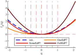
Figure 3: Range reshaping function before (dashed blue) and after (solid) optimization.

Remark 5

Fig. 1 illustrates the change in trajectories our optimization yields. Note that in the bearing-only case (left images), the lack of a fixed scale led to an overall shrinking of the formation to reduce the total path length. This is avoided by including range terms (right images).

V-B Performance evaluation

We tested the optimized reshaping function in Figs. 2,3 using 200 randomly selected initial conditions for the agents (called the Test set). Performance was evaluated using five metrics. The first was the path length $L_{\textrm{path}}(\mathbf{\alpha},\mathbf{x}_{0})$, defined by (19) without the terminal condition (see Remark 3). The second was the difference of the path length from a straight line,

$$L_{\textrm{diff}}(\mathbf{\alpha},\mathbf{x}_{0})=L_{\textrm{path}}(\mathbf{\alpha},\mathbf{x}_{0})-\sum_{i\in\mathcal{V}}\lVert x_{i}(T)-x_{i}(0)\rVert.$$ (42)

The other two were the corresponding percentage of relative improvement:

$$\delta path=100\frac{L_{\textrm{path}}(\mathbf{\alpha}_{\textrm{init}})-L_{\textrm{path}}(\mathbf{\alpha}_{\textrm{opt}})}{L_{\textrm{path}}(\mathbf{\alpha}_{\textrm{init}})},$$ (43)

$$\delta diff=100\frac{L_{\textrm{diff}}(\mathbf{\alpha}_{\textrm{init}})-L_{\textrm{diff}}(\mathbf{\alpha}_{\textrm{opt}})}{L_{\textrm{diff}}(\mathbf{\alpha}_{\textrm{init}})}.$$ (44)

We also define scale of a formation as the standard deviation (STD) of the positions of the agents in the formation.

TABLE I: Summary of performance. Results for $\delta{path}$ and $\delta{diff}$ are reported as mean values over the trials of the training and test data, with higher numbers indicating better performance. For the test data, the medians for these metrics are also reported in parentheses. In addition, the test data results include the mean for the path length, with lower numbers indicating better performance. The final column is the percentage of trials in the test data for which path length improved.

Case	Model		Training		Test
			$\delta path$ (%)	$\delta diff.$ (%)	$L_{\textrm{path,init}}$	$L_{\textrm{path,opt}}$	$\delta path$(%)	$\delta diff.$(%)	$+$%
Train on 5 Test on 5	NoEd	1 ICs	24.35	54.36	45.17	40.79	8.72 (9.46)	0.94 (11.28)	81
		3 ICs	8.47	20.61	45.17	40.98	8.6 (8.43)	12.68 (16.05)	87
		5 ICs	7.43	17.72	45.17	41.37	7.82 (7.57)	11.9 (15.84)	87.5
		7 ICs	7.26	22.04	45.17	41.38	7.87 (7.45)	15.7 (19.76)	90
	OneEd	7 ICs	3.75	23.03	52.39	50.11	4.09 (4.32)	22.58 (24.05)	90
	SomeEd	7 ICs	11.02	53.67	52.79	47.82	9.14 (9)	49.42 (52.83)	97.5
	FullEd	7 ICs	11.05	61.15	52.07	46.13	11.26 (11.73)	65.64 (67.78)	99.5
Train on 5 Test on 5 Alt.shape	NoEd	7 ICs	7.26	22.04	45.41	41.24	8.8 (8.19)	22.7 (21.9)	95.5
	OneEd	7 ICs	3.75	23.03	49.75	47.64	4.02 (4.25)	21.56 (22.11)	89
	SomeEd	7 ICs	11.02	53.67	50.4	46.31	7.91 (8.28)	39.12 (39.99)	94
	FullEd	7 ICs	11.05	61.15	47.98	43.48	9.16 (9.52)	56.55 (59.62)	99
Train on 5 Test on 3	NoEd	7 ICs	7.26	22.04	21.53	19.43	8.76 (7.91)	29.38 (37.79)	93
	OneEd	7 ICs	3.75	23.03	28.78	26.93	5.97 (6.25)	40.5 (47.31)	92.5
	SomeEd	7 ICs	11.02	53.67	28.78	26.75	6.44 (6.75)	40.54 (52.07)	91
	FullEd	7 ICs	11.05	61.15	28.96	25.21	12.66 (14.14)	87.53 (92.07)	99.5

The results on the Training and Test sets under the different controllers are summarized in Table I. Several trends emerge from these results:

• From the Training set, we see that increasing the number of initial conditions decreases the improvement. This makes intuitive sense since the algorithm is looking for the best performance averaged over more conditions.

• As expected, there is gap between training and testing performance. However this gap diminishes as we increase the number of initial conditions considered in the optimization. These results imply that the reshaping function that yields the shortest path depends on where an agent starts but that averaging over a few initial conditions ensures reasonable performance across a wide range of start locations. As seen in the last column, when using seven initial conditions in training, over 90% of the initial conditions in the test set showed a reduction in path length.

• Performance improves as additional edges are added to the controller. This likely arises from the additional information available in the extra range measurements.

• The four rows afterwards indicate that the training results can transfer well to a other formations, yielding similar improvements in the trajectories (see Fig.4 for an example). The last four rows show that the training results transfer to a 3-agent system as well. Interestingly, with full range data and three agents (final row), the results are very close to straight lines, reaching nearly 90% relative improvement.

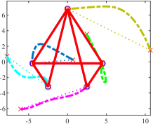
(a)

(b)

Figure 4: Bearing-based 5-agent system where $E_{b}=E_{d}$ with alternate goal configuration. (a) before optimization. (b) after.

V-C Comparison with Other Controllers

To further demonstrate the performance of our method, we compare it with other methods under both the bearing-only and bearing+range conditions:

1. bearing-only (’NoEd’) formation controller: we compare with [22, eq. (8)], a distributed bearing-only formation control law that uses a Lyapunov approach.

2. bearing+range ($|\mathcal{E}_{d}|=|\mathcal{E}_{b}|$, ’FullEd’) formation controller: we compare with [23, 10, eq. (5)], a distributed bearing-based formation control law that uses relative position measurements and assumes two independently controlled leaders. Note that we adapt our controller to the leader-follower case by simply fixing the position of the leaders (while still training in the leaderless case).

The results in Table II show that our method yields shorter trajectories, and that the parameters learned from our leaderless optimization are still effective when a leader is considered, despite the fact that [23] actually requires the presence of leaders.

TABLE II: Comparison: NoEd.Init. and NoEd.Opt. are the bearing-only controllers before and after optimization using 7ICs, while FullEd.Init. and FullEd.Opt. are the ones for bearing+range case. To allow a fair comparison with [23], methods marked with ^⋆ fix the position of two leaders. The reported statistics have the same meaning as in Table I Test.

	$L_{\textrm{path,A}}$	$L_{\textrm{path,B}}$	$\delta path$(%)	$\delta diff.$(%)	$+$%
A: Zhao B: NoEd.Init.	65.9	45.2	29 (28.4)	51.2 (55.4)	100
A: Zhao B: NoEd.Opt.	65.9	41.4	34.1 (34.1)	58.2 (63.6)	99.5
A⋆: Zhao B⋆: FullEd.Init.	35.5	30.7	12.8 (12.9)	42.9 (7.2)	94.5
A⋆: Zhao B⋆: FullEd.Opt.	35.5	29.5	16.3 (16.9)	58 (56)	98.5

VI Conclusions

In this paper, we formulated a nonlinear optimization problem on a gradient-descent bearing-based formation controller, which utilizes a reshaping function to embed the relationship between the current and desired bearing. We simulated the algorithms in Matlab to evalulate their performance on a 5-agent network. The optimization consistently led to the same qualitative form of the reshaping function for bearing-only (NoEd) and full range (FullEd) cases, though the pattern did not hold for the one-range (OneEd) case. By applying the optimized reshaping function, the bearing-only path length $L_{\textrm{path}}$ was shortened by around 8% and the difference to straight lines $L_{\textrm{diff}}$ was improved by $\sim$16% in these simulations. In addition, with radomized initial conditions, over 90% of the trials runs showed improvement relative to the non-optimized case. Our results indicate that using a larger training set in the optimization leads to a small reduction in performance gain but a significant improvement on maintaining the scale of the formation. By introducing more range terms, both the training and test performance improved, up to 11.3% in $L_{\textrm{path}}$ and 65.6% in $L_{\textrm{diff}}$. More over, almost all the test samples benefited from the optimization despite the small training set. It is also promising to see that the training result on 5-agent network can be generalized to other formations and networks with different numbers of agents. For future work, we are planning to (1) use the basic form of the optimized reshaping function to reduce the number of control points needed and thus reduce the complexity of the optimization problem, (2) generalize the optimization approach to include different dynamic models for the agents, (3) propose a collision avoidance solution to remove the problem arising when the range between two agents goes to zero.

APPENDIX

VI-A Proof of Lemma 2

Given (1), (2) and (6), we see that $d_{ij}$, $\beta_{ij}$, and $\varphi_{ij}^{b}$ are invariant to an arbitrary translation $t_{ij}$ (i.e. $d(x_{i}+t_{ij},x_{j}+t_{ij})=d(x_{i},x_{j})$, $\beta(x_{i}+t_{ij},x_{j}+t_{ij})=\beta(x_{i},x_{j})$, $\varphi(x_{i}+t_{ij},x_{j}+t_{ij})=\varphi(x_{i},x_{j})$). Therefore,

$$\begin{split}\varphi_{ij}^{b}(\tilde{x}_{i}(t),\tilde{x}_{j}(t))&=\varphi_{ij}^{b}(0,\tilde{x}_{j}(t)-\tilde{x}_{i}(t))\\ &=\varphi_{ij}^{b}(0,t(v_{j}-v_{i})).\end{split}$$ (45)

Then, we can move and scale the desired configuration $x_{g,i}$ and $x_{g,j}$ such that $x_{g,i}=(0,0)$, $x_{g,j}=(1,0)$, and $\beta_{g,ij}=(1,0)$. Given $c_{ij}=\beta_{g,ij}^{T}\beta_{ij}$, we define $v_{j}-v_{i}=(c_{ij},\sqrt{1-c_{ij}^{2}})=\beta_{ij}$. Letting $v_{i}=(0,0)$, $v_{j}=(c_{ij},\sqrt{1-c_{ij}^{2}})$, and fixing agent $i$, the original evaluation on $(\tilde{x}_{i}(t),\tilde{x}_{j}(t))$ is simplified to evaluate the location of agent $j$ on a radial line starting from the origin. Here, varying $v_{j}$ is analogous to varying the bearing vector of agent $i$ and $j$ in a unit circle centering at the origin.

It then follows that on the parametric line $(0,tv_{j})$, we have

$$v_{j} =\frac{\tilde{x}_{j}-\tilde{x}_{i}}{\lVert\tilde{x}_{j}-\tilde{x}_{i}\rVert}=\tilde{\beta}_{ij},$$ (46)

$$\dot{\tilde{d}}_{ij} =\frac{d}{dt}\lVert tv_{j}-0\rVert=v_{j}^{T}\tilde{\beta}_{ij}.$$ (47)

Given we are evaluating the terms along a bearing direction, the derivative of $\tilde{\beta}_{ij}$ on $t$ is a zero vector, and the corresponding $\dot{\tilde{c}}_{ij}=\beta_{g,ij}^{T}\dot{\tilde{\beta}}_{ij}$ is also zero. Then,

$$\begin{split}\dot{\tilde{\varphi}}_{ij}^{b}&=f_{b}(\tilde{c}_{ij})\dot{\tilde{d}}_{ij}+\dot{f}_{b}(\tilde{c}_{ij})d_{ij}\dot{\tilde{c}}_{ij}=f_{b}(\tilde{c}_{ij})v_{j}^{T}\tilde{\beta}_{ij}\\ &=f_{b}(\tilde{c}_{ij})\tilde{\beta}_{ij}^{T}\tilde{\beta}_{ij}=f_{b}(\tilde{c}_{ij}).\end{split}$$ (48)

Given the constraint (13) on $f_{b}(\cdot)$, we have $\dot{\tilde{\varphi}}^{b}_{ij}(t)\geq 0,\text{ with equality if and only if }c_{ij}=1$.

VI-B Insensitive Weights in the Optimization Objective Terms

To see this, note that we do not have a regularization term on $\alpha$. As a consequence, we expect that the second term with $\varphi(x(T))$ in the cost (19) will always be negligible for any reasonable choice of $\omega$. This is because $f_{b}(\cdot)$, $f^{\prime}_{b}(\cdot)$, and hence the control $\mathbf{u}$, are homogeneous in $\alpha$, which means by scaling $\alpha$ we can maintain the same paths $\mathbf{x}(t)$, but change the speed; this then implies that the first term in (19) does not depend on the scale of $\alpha$, but only on its direction. If, by way of contradiction, we had a solution $\alpha_{\textrm{opt}}$ which was optimal but for which $\varphi(\mathbf{x}(T)\gg 0$, then we could simply augment the scale of $\alpha$ to make the agents go faster, thus reducing the total cost, giving a contradiction with the fact that $\alpha_{\textrm{opt}}$ is optimal.

VI-C Possible Solution of Discontinuous Sensitivity Funtion

A (possibly) better approach to handle the discontinuity when the range between two agents goes to zero is to introduce a bump function $\phi(d_{i})=\prod_{(i,j)\in\mathcal{E}_{b}}\phi_{e}(d_{ij})$ where $d_{i}=\{d_{ij}\}_{j:(i,j)\in\mathcal{E}_{b}}$ indicates the ranges to all agents connected to agent $i$, and

$$\phi_{e}(d_{ij})=\begin{cases}1-\exp(1+\frac{1}{(\frac{d_{ij}}{\epsilon})^{2p}-1}),&\text{if $d_{ij}<\epsilon$},\\ 1,&\text{otherwise},\end{cases}$$

where $\epsilon>0$ is a given small number and $p$ is an appropriate power. We then modify the path length into $\int^{T}_{0}\phi(d_{i})||\dot{x}_{i}(\mathbf{x}(t),\mathbf{\alpha)}||\mathrm{d}t$.

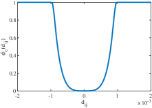
(a)

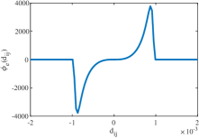
(b)

Figure 5: Bump Function ($p=2$, $\epsilon=10^{3}$)

Since $\phi$ and its derivative are both well behaved (and zero) as two agents move through a common point, including this function should help the sensitivity well-behaved. Intuitively, because the bump function drives the path length term to zero independent of $\alpha$, the integral can be broken into two terms, one before and one after the intersection of the agents. Making this idea rigorous is a topic of ongoing research.

References

- [1] B. D. O. Anderson, B. Fidan, C. Yu, and D. Walle, “UAV formation control: Theory and application,” in Recent Advance in Learning and Control, ser. Lecture Notes in Control and Information Sciences, vol. 371. Springer, 2008, pp. 15–33.
- [2] N. Michael, J. Fink, and V. Kumar, “Cooperative manipulation and transportation with aerial robots,” Autonomous Robots, vol. 30, pp. 73–86, 2011.
- [3] A. Petitti, A. Franchi, D. D. Paola, and A. Rizzo, “Decentralized motion control for cooperative manipulation with a team of networked mobile manipulators,” in IEEE Int. Conf. on Robot. Automat., 2016, pp. 441–446.
- [4] K. K. Oh, M. C. Park, and H. S. Ahn, “A survey of multi-agent formation control,” Automatica, vol. 53, pp. 424 – 440, 2015.
- [5] A. N. Bishop, I. Shames, and B. Anderson, “Stabilization of rigid formations with direction-only constraints,” in IEEE Int. Conf. on Decision and Control, 2011, pp. 746–752.
- [6] A. N. Bishop, T. H. Summers, and B. D. O. Anderson, “Stabilization of stiff formations with a mix of direction and distance constraints,” in IEEE Int. Conf. on Contr. Appl., 2013, pp. 1194–1199.
- [7] A. N. Bishop, M. Deghat, B. D. O. Anderson, and Y. Hong, “Distributed formation control with relaxed motion requirements,” International Journal of Robust and Nonlinear Control, vol. 25, no. 17, pp. 3210–3230, 2015.
- [8] A. Franchi, C. Masone, V. Grabe, M. Ryll, H. H. Bülthoff, and P. R. Giordano, “Modeling and control of UAV bearing formations with bilateral high-level steering,” International Journal of Robotics Research, vol. 31, no. 12, pp. 1504–1525, 2012.
- [9] S. Zhao and D. Zelazo, “Bearing rigidity and almost global bearing-only formation stabilization,” IEEE Trans. Automat. Contr., vol. 61, no. 5, pp. 1255–1268, 2016.
- [10] ——, “Bearing rigidity theory and its applications for control and estimation of network systems: Life beyond distance rigidity,” IEEE Control Syst. Mag., vol. 39, no. 2, pp. 66–83, 2019.
- [11] R. Tron, J. Thomas, G. Loianno, K. Daniilidis, and V. Kumar, “Bearing-only formation control with auxiliary distance measurements, leaders, and collision avoidance,” in IEEE Int. Conf. on Decision and Control, 2016, pp. 1806–1813.
- [12] R. Tron and K. Daniilidis, “An optimization approach to bearing-only visual homing with applications to a 2-d unicycle model,” in IEEE Int. Conf. on Robot. Automat., 2014, pp. 4235–4242.
- [13] R. Tron, “Bearing-based formation control with second-order agent dynamics,” in IEEE Int. Conf. on Decision and Control, 2018, pp. 446–452.
- [14] S. Zhao, Z. Li, and Z. Ding, “A revisit to gradient-descent bearing-only formation control,” in IEEE Int. Conf. on Contr. Automat, 2018, pp. 710–715.
- [15] ——, “Bearing-only formation tracking control of multiagent systems,” IEEE Trans. Automat. Contr., vol. 64, no. 11, pp. 4541–4554, 2019.
- [16] A. Karimian and R. Tron, “Bearing-only consensus and formation control under directed topologies,” in American Control Conference, 2020, pp. 3503–3510.
- [17] J. Zhao, X. Yu, X. Li, and H. Wang, “Bearing-only formation tracking control of multi-agent systems with local reference frames and constant-velocity leaders,” IEEE Control Systems Letters, vol. 5, no. 1, pp. 1–6, 2021.
- [18] S. Leonardos, K. Daniilidis, and R. Tron, “Distributed 3-d bearing-only orientation localization,” in IEEE Int. Conf. on Decision and Control, 2019, pp. 1834–1841.
- [19] R. L. Burden and J. D. Faires, Numerical Analysis, 9th ed. Brooks/Cole, Cengage Learning, 2011.
- [20] P. T. Boggs and J. W. Tolle, “Sequential quadratic programming,” Acta Numerica, vol. 4, no. 1, pp. 1–51, 1995.
- [21] H. K. Khalil and J. W. Grizzle, Nonlinear systems, 3rd ed. Prentice hall Upper Saddle River, NJ, 2002.
- [22] S. Zhao and D. Zelazo, “Bearing rigidity and almost global bearing-only formation stabilization,” IEEE Transactions on Automatic Control, vol. 61, no. 5, pp. 1255–1268, 2016.
- [23] ——, “Bearing-based distributed control and estimation of multi-agent systems,” in 2015 European Control Conference (ECC), 2015, pp. 2202–2207.