Low X-ray surface brightness clusters: Implications on the scatter of the $M-T$ and $L-T$ relations

Abstract

We aim at studying scaling relations of a small but well defined sample of galaxy clusters that includes the recently discovered class of objects that are X-ray faint for their mass. These clusters have an average low X-ray surface brightness, a low gas fraction and are under-represented (by a factor of 10) in X-ray surveys or entirely absent in SZ surveys. With the inclusion of these objects, we find that the temperature-mass relation has an unprecedented large scatter, $0.20\pm 0.03$ dex at fixed mass, as wide as allowed by the temperature range, and the location of a cluster in this plane depends on its surface brightness. Clusters obey a relatively tight luminosity-temperature relation independently of the their brightness. We interpret the wide difference in scatter around the two relations as due to the fact that X-ray luminosity and temperature are dominated by photons coming from small radii (in particular for $T$ we used a 300 kpc aperture radius) and strongly affected by gas thermodynamics (e.g. shocks, cool-cores), whereas mass is dominated by dark matter at large radii. We measure a slope of $2.0\pm 0.2$ for the $L_{500}-T$ relation. Given the characteristics of our sample, this value is free from the collinearity (degeneracy) between evolution and slope and from hypothesis on the undetected population, that both affect the analysis of X-ray selected samples, and can therefore be profitably used both as reference and to break the above degeneracy of X-ray selected-samples.

1 Introduction

Under thermodynamic equilibrium condition, the temperature of an isolated isothermal sphere of ideal gas is determined by the depth of the sphere potential well, $T\propto M^{2/3}$, also known as self-similar scaling, with no scatter and no covariance with any other quantity, (Kaiser 1986). Deviations from this ideal behaviour, in particular intercept and slope of the mean relation, the scatter around the mean relation, and its covariance with other parameters, can be used to gather information about the processes that shape galaxy clusters (e.g. Yang et al. 2009). Pre-heating and cooling might alter the slope of the scaling relation (Stanek et al. 2010); cooling, star formation and feedback might alter both slope and intercept (Fabjan et al. 2010), while cooling and star formation might introduce a scatter (Nagai et al. 2007a). The variety of the mass accretion histories may also introduce a scatter and an offset (Yang et al. 2009, Ragagnin & Andreon 2022), and the offset from the mean relation is covariant with other cluster properties, such as concentration or formation redshift (Yang et al. 2009) or mass acretion history (Chen et al. 2019).

Observationally, the mass-tempertature scaling is found to be quite tight (with a scatter not exceeding 20% at most; Arnaud et al. 2005; Vikhlinin et al. 2006; Zhang et al. 2006, 2007; Lovisari et al. 2020), but past studies suffer from several limitations in the samples used or in the analyses applied. All, or almost all, samples used to measure mass-temperature scaling studied so far are either a collection of objects or are X-ray- or SZ-selected. These samples lacks clusters of low surface brightness (Pacaud et al. 2007; Andreon & Moretti 2011; Eckert et al. 2011; Planck Collaboration 2011, 2012; Andreon et al. 2016, 2022; O’Sullivan et al. 2017, Pearson et al. 2017, Xu et al. 2018; Orlowski-Scherer et al. 2021). Andreon et al. (2022) shows that cluster X-ray faint for their mass, or equivalently of low surface brightness are underrepresented by a factor of 10 in X-ray surveys and are entirely missing in SZ surveys. If the missed population obeys a different scaling law than the observed one (e.g., has a lower intercept, a different slope, or a wider scatter), it is not possible to recover the parameters of the entire population when no or too few examples of the missing one are present in the sample. Therefore results based on such samples, when corrected for sample selection (e.g. Giles et al. 2016; Liu et al. 2016; Chiu et al. 2022), necessarely implicitly assume that the missed population obeys the same scaling relation as the one observed. Furthermore, very often hydrostatic masses are used (e.g. Arnaud et al. 2005, Viklinin et al. 2007), which restrict the sample to relaxed clusters only because the hydrostatic equilibrium might not be correct for unrelaxed clusters. In simulations, un-relaxed clusters show a different scatter (Nagai 2007b), further suggesting that the mass-temerature relation based on relaxed clusters is biased.

The soundness of the analysis is often hampered by the fitting methods used. Many works in the past have used simplified fitting methods that did not account for the sample selection function and the non-constant mass function (see Andreon & Hurn 2013 for a review on statistical issues related to scaling relations). Furthermore, hydrostatic masses (Sarazin 1988), widely used for mass-temperature scaling relations, are, by definition, derived directly from $T$ and therefore they cannot be considered independent from it, in spite of what most analyses performed thus far assume. This introduces possible biases, the most obvious of which is an underestimate of the scatter around the mean relation because the covariance in the errors is neglected (see also Zhang et al. 2006). Masses estimated from gas masses, gas fraction, or $Y_{X}$ (Kravtsov et al. 2006) have similar shortcomings, as discussed in Sec. 3. When the clusters considered have different redshifts, as it is often the case, there is a degeneracy between the evolution and slope of the scaling relation, as discussed in detail in Sec. 4.

A sample selected independently of the intracluster medium being studied and with known masses would allow us to directly see where the population of clusters missed by X-ray and SZ-selected samples falls in the mass-temperature diagram, and therefore to unveil weather this hard-to-detect population obeys the same mass-temperature scaling relation as the one determined from current samples. The X-ray Unbiased Cluster Sample (XUCS, Andreon et al. 2016) is ideal for this purpose since its selection is independent of the intracluster medium, it contains a sizeable fraction of these low X-ray surface brightness clusters and masses are not measured from the X-ray photons used to infer temperature, therefore making the estimates of temperature and mass independent.

Throughout this paper, we assume $\Omega_{M}=0.3$, $\Omega_{\Lambda}=0.7$, and $H_{0}=70$ km s^-1 Mpc^-1. Results of stochastic computations are given in the form $x\pm y$, where $x$ and $y$ are the posterior mean and standard deviation. The latter also corresponds to 68% uncertainties because we only summarize posteriors close to Gaussian in this way. All logarithms are in base 10.

2 The sample and the measurements

The XUCS sample consists of 34 clusters in the very nearby universe ($0.050<z<0.135$) selected from the SDSS spectroscopic survey using more than 50 concordant redshifts whithin 1 Mpc and a velocity dispersion of members $\sigma_{v}>500$ km/s (see Paper I and Paper II). They are in regions of low Galactic absorption, by design. There is no X-ray selection in the sample in the sense that the probability of inclusion of a cluster is independent of its X-ray luminosity, or any X-ray property, and no cluster is added/removed on the basis of its X-ray luminosity. All clusters were followed-up in the X-ray band with Swift, except for a few with adequate XMM-Newton or Chandra data in the archives.

Caustic masses (Diaferio & Geller 1997 and later works), that have the advantage of not relying on the dynamical equilibrium hypothesis, were derived within $r_{200}$ in Paper I, using more than 100 galaxy velocities, on average, per cluster, and then converted into masses within $r_{500}$, $M_{500}$, assuming a Navarro et al. (1997) profile with concentration five (using a value of three would not have changed the results, see Paper I). The average mass error is 0.14 dex. In our sample, we found that caustic masses are consistent with dynamical and weak-lensing masses (Paper I and III), and for a single cluster with a deep X-ray follow-up, also with the hydrostatic mass (Paper IV). In other samples, caustic masses are, in general, found to agree with weak-lensing masses and hydrostatic masses (Geller et al. 2013, Hoekstra et al. 2015, Maughan et al. 2016).

Table 1: Results of the analysis.

Id	RA	Dec	z	$T_{X}(r<300)$
	(J2000)			keV
CL1001	208.2560	5.1340	0.079	$5.7^{0.4}_{-0.3}$
CL1009	198.0567	-0.9744	0.085	$3.1^{0.2}_{-0.2}$
CL1011	227.1073	-0.2663	0.091	$2.9^{0.8}_{-0.6}$
CL1014	175.2992	5.7350	0.098	$3.3^{0.4}_{-0.4}$
CL1015	182.5701	5.3860	0.077	$3.9^{0.2}_{-0.2}$
CL1018	214.3980	2.0530	0.054	$2.4^{0.6}_{-0.4}$
CL1020	176.0284	5.7980	0.103	$5.0^{0.7}_{-0.6}$
CL1030	206.1648	2.8600	0.078	$1.6^{0.2}_{-0.2}$
CL1033	167.7473	1.1280	0.097	$2.8^{0.6}_{-0.5}$
CL1038	179.3788	5.0980	0.076	$4.7^{0.9}_{-0.7}$
CL1039	228.8088	4.3860	0.098	$6.0^{0.4}_{-0.3}$
CL1041	194.6729	-1.7610	0.084	$6.2^{0.1}_{-0.1}$
CL1047	229.1838	-0.9693	0.118	$7.1^{1.9}_{-1.4}$
				$5.1^{0.1}_{-0.1}$
CL1052	195.7191	-2.5160	0.083	$3.5^{0.1}_{-0.1}$
CL1067	212.0220	5.4180	0.088	$3.6^{0.7}_{-0.4}$
CL1073	170.7265	1.1140	0.074	$2.7^{0.4}_{-0.2}$
				$3.0^{0.6}_{-0.5}$
CL1120	188.6107	4.0560	0.085	$1.2^{0.2}_{-0.2}$
CL1132	195.1427	-2.1340	0.085	$1.4^{0.2}_{-0.2}$
CL1209	149.1609	-0.3580	0.087	$2.1^{0.1}_{-0.1}$
CL2007	46.5723	-0.1400	0.109	$1.6^{0.6}_{-0.2}$
CL2010	29.0706	1.0510	0.080	$2.6^{0.4}_{-0.3}$
CL2015	13.9663	-9.9860	0.055	$3.7^{1.3}_{-0.9}$
CL2045	22.8872	0.5560	0.079	$2.7^{0.5}_{-0.3}$
CL3000	163.4024	54.8700	0.072	$2.5^{0.2}_{-0.2}$
CL3009	136.9768	52.7900	0.099	$1.5^{0.2}_{-0.2}$
CL3013	173.3113	66.3800	0.115	$5.3^{0.7}_{-0.4}$
CL3020	232.3110	52.8600	0.073	$3.6^{0.7}_{-0.6}$
CL3023	122.5355	35.2800	0.084	$4.5^{1.4}_{-1.1}$
CL3030	126.3710	47.1300	0.127	$7.0^{0.8}_{-0.6}$
CL3046	164.5986	56.7900	0.135	$10.8^{2.0}_{-1.2}$
				$10.7^{1.2}_{-0.8}$
CL3049	203.2638	60.1200	0.072	$2.9^{0.5}_{-0.3}$
CL3053	160.2543	58.2900	0.073	$2.5^{1.8}_{-0.8}$

Three clusters have been observed by two telescopes and therefore are listed twice. Coordinates and redshifts are from Paper I.

The X-ray data reduction is described in Paper I. Briefly, we reduced the X-ray data (mostly Swift, but also Chandra and XMM-Newton, with three clusters observed by Swift and either XMM-Newton or Chandra) using the standard data reduction procedures (Moretti et al. 2009; XMMSAS 2 or CIAO 3). In paper I we derived $L_{500}$, the cluster X-ray luminosity within $r_{500}$, and its core-excised version $L_{500,ce}$, calculated excluding radii smaller than $0.15r_{500}$. To have a glimpse on the spread of the quality of the determinations, the median X-ray luminosity error is 0.04 dex, the error interquartile range is (0.02,0.06) dex, the worst determination has 0.15 dex error. We took the position of the brightest cluster galaxy closest to the X-ray peak as the cluster center.

One cluster, CL1022, is bimodal and therefore measuring its central temperature is meaningless. Another cluster, CL2081, is too faint to derive a robust measurement of the temperature. For these reasons, these two clusters were dropped from the sample that we will use in next sections.

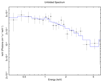
Figure 1: Example spectrum. The figure shows the spectrum of the cluster CL1038, which has median value of net photons in the spectroscopic aperture.

Here, we measure the X-ray temperature within a 300 kpc aperture following the same procedure adopted for temperature measurements in a larger aperture in Paper II: first, we extracted photons in [0.3-7] keV band in two regions, $r<300$ kpc and the annulus between $r/r_{500}=0.7$ and the 50% exposure boundary. As discussed in Paper II, the background annulus is far enough not to bias the X-ray temperature determination. The source spectrum was fit with an absorbed APEC (Smith et al. 2001) plasma model, with the absorbing column fixed at the Galactic value (Dickey & Lockman 1990), the metal abundance fixed at 0.3 relative to solar, and the redshift of the plasma model fixed at the optical redshift. The fit accounts for variations in exposure time, excised regions, etc. The spectrum was grouped to contain a minimum of five counts per bin and the source and background data were fitted within the XSPEC (Arnaud 1996) spectral package using the modified C-statistic (also called W-statistic in XSPEC). The median number of net photons within the aperture is 712 (interquartile range $=$(404,2365)). Cluster photons are, on average, 60% of all photons in the aperture because of the low background of XRT and because XRT is used for almost all clusters. The median temperature error is 15%. The error interquartile range is (9,20)%. We find consistent temperature values for the three clusters observed with XRT and Chandra or XMM-Newton (with a difference of $<1.4\sigma$).

Table 1 lists derived temperatures. An example of the “average" quality of the spectral data is given in Fig. 1, where we show the spectrum of CL1038 that contains the median value of net photons.

3 Results

3.1 $L_{X}-M$

The XUCS $L_{X}-M$ relation was presented and discussed in Paper I. In Fig. 2 we show it again, here color coded by the offset from the mean relation. The Figure also shows the mean relation and the $\pm 1\sigma_{\text{intr}}$ regions for the X-ray selected REXCESS sample (Bohringer et al. 2007) with the green solid line and the dashed corridor. The XUCS sample (data points) occupies a much wider portion of the $L_{X}-M$ plane than REXCESS, as discussed in Paper I. Blue points represent under-luminous clusters (faint for their mass), red ones are over-luminous. The offset can also be read as a difference in the average surface brightness within $r_{500}$: clusters 1 dex brighter in $L_{500,ce}$ are also 1 dex brighter in average surface brightness compared to clusters with the same $r_{500}$ (or $M_{500}$), by definition. A pair of such clusters is shown in Fig. 2 and 4 of Paper I. Paper II shows these differences to be related to gas fraction: clusters that are X-ray faint for their mass are also gas poor. Furthermore, once X-ray luminosity is corrected by gas fraction, the X-ray luminosity vs mass scaling become almost scatterless (Paper II). In other terms, the color coding indicates equivalently a difference in X-ray luminosity, in mean surface brightness within $r_{500}$, or in gas fraction at fixed mass. In the Figures we use $\Delta\log L_{500,ce}|M$ (the vertical bar reads “at") which is more directly related to the data, but we could have equally used $\Delta\log f_{gas}|M$ or $\Delta\log\mu_{r_{500}}|M$. The two clusters dropped from further analysis are identified with a square.

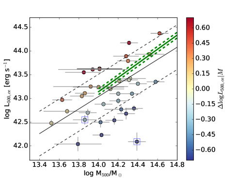
Figure 2: The sample. Core-excised luminosity within $r_{500}$ in the [0.5-2] band vs $M_{500}$ color-coded by offset from the mean relation. The two objects excluded by the current analysis are marked by squares. The blue solid line and the dashed corridor indicate the mean relation and the $\pm 1\sigma_{\text{intr}}$ regions derived in Paper I and II. Three clusters (observed by two telescopes) appear twice in the figure, although distinguishing these duplicates in the plot can be sometime challenging. The green solid line and the dashed corridor indicate the mean relation and the $\pm 1\sigma_{\text{intr}}$ regions derived for the X-ray selected REXCESS sample.

3.2 $T-M$

Fig. 3 shows the XUCS sample in the mass-temperature plane. In place of the common tight relation, the sample shows a relatively large scatter and shows that the location of a cluster in the plot is closely related to the offset from the $L_{500,ce}-M$ mean relation: blue points are systematically below red points. As will be illustrated below, this occurs because $T$ is directly related to $L_{X}$ and only indirectly to $M$.

To derive the scatter, we adopt Gaussian errors in $\log M_{500}$ and lognormal errors on $T_{X}$ (introduced in Andreon 2012 and now widely adopted) and a Gaussian intrinsic scatter in $\log T|M$. For the three clusters with observations with two telescopes, we use the measure with smaller errors. We adopt weak priors for the parameters and a uniform prior in $\log M$. Since the sample is not X-ray selected, we don’t need to model the X-ray selection function and to make hypothesis on the amplitude and spread of the unseen population. The numerical implementation of the code is given in Sec. 8.4 of Andreon & Weaver (2015). We found

$$\log T=(0.42\pm 0.14)(\log M_{500}-14.2)+0.59\pm 0.04$$ (1)

where $T$ is in keV and $M_{500}$ is in $M_{\odot}$. The intrinsic scatter is $0.20\pm 0.03$ dex at fixed mass and there is almost no covariance between parameters because of our choice of pivoting masses near the middle of the data distribution (i.e. subtracting 14.2 to $\log M_{500}$). The intrinsic scatter is maximally large since the data scatter in $T$ is 0.22 dex. An identical result is obtained by taking a Schechter (1976) as prior mass function, basically because the errors on $M$ are small compared to the prior width for almost all data points. This indicates that our results are independent of the shape of the $M$ distribution adopted for the sample.

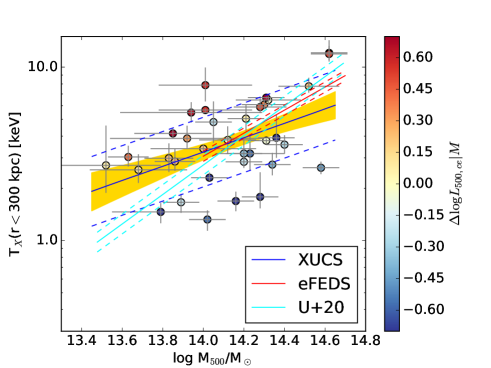
Figure 3: Temperature-Mass relation color-coded by the offset from the mean $L_{X,ce}-M$ relation. The mean model and its 68% error are shown as a blue solid line and yellow shading, respectively. Clusters faint for their $M_{500}$ (blue points) have a systematically cooler temperature for their mass. Three clusters (observed by two telescopes) appear twice in the figure. Fits from the literature are also shown, with 68% corridors indicated by dashed lines, which severely underestimate the spread observed in the XUCS sample.

Fig. 3 also shows two determinations of the mass-temperature relation from the literature which use, as we do, non-core-excised temperatures. Both use weak-lensing masses from the Hyper Suprime-Cam Subaru Strategic Program survey (Aihara et al. 2018) and X-ray selected samples: Umetsu et al (2020, cyan in the figure) use the XXL survey (Pierre et al. 2016), whereas Chiu et al. (2022, red in the figure) uses the eROSITA Final Equatorial-Dept survey (eFEDS, Liu et al. 2022). Umetsu et al (2020) use $T(<300)$ kpc, as we do, whereas Chiu et al. (2022) use $T_{(}<r_{500}$) found by Giles et al. (2016) to be indistinguishable from $T(<300)$ kpc given the errors. Umetsu et al (2020) and Chiu et al. (2022) find an intrinsic scatter of $0.06\pm 0.05$ and $0.03^{+0.03}_{-0.01}$ dex at fixed mass, respectively vs $0.20\pm 0.03$ dex for XUCS. In Fig. 3 dashed corridors mark the $\pm 1\sigma_{intr}$ region around the mean relation, which in absence of errors include 68% of the data points. These two relations and reported scatter severely underestimate the scatter observed in XUCS. This occurs because both XXL and eFEDS lack clusters of low surface brightness (the blue and cyan points) and therefore from these data it is not possible to recover the full size of the mass-temperature distribution and to properly estimate the region occupied by low surface brightness clusters from the detected clusters with high surface brightness. The slope of the mass-temperature relation is very poorly determined in Umetsu et al. (2020) because the errors on the mass are larger than the explored mass range, while Liu et al. (2022) slope determination assumes that clusters of all brightnesses obey a brightness-independent mass-temperature scaling, which XUCS data manifestly show not to be true. These discrepancies emphasize the importance of using cluster samples inclusive of low surface brightness objects and of developing fitting schemes that allows us to properly infer the spread of the population when a part of it is severely undersampled, as in X-ray surveys.

More in general, the unprecedent large spread observed in the XUCS sample does not show up in X-ray or SZ selected samples for two reasons. First, as mentioned, because they rarely include low luminosity/low surface brightness clusters (namely the blue points, see Andreon et al. 2016,2022). Second, the observed scatter is strongly reduced by assuming a scatterless scaling relation to infer the radius $r_{500}$ in which measurements have to be performed. For example, in analyses where $r_{500}$ is estimated from $T$ (e.g., Giles et al. 2016), a cluster of low/high temperature for its mass will have an estimated $r_{500}$ appropriate to put it precisely on the mean $M_{500}-T$ relation because this same relation, in the mathematically equivalent $r_{500}-T$ form, is used to infer $r_{500}$ from $T$. With this assumption, cold clusters are forced to have a small $r_{500}$ and therefore to be of low mass, even when the low temperature is related to low luminosity and surface brightness. Similarly, if mass is estimated assuming that all clusters share the same gas fraction (e.g. Mantz et al. 2010), it will again be underestimated for clusters of low surface brightness (gas fraction). The assumption of an average gas fraction moves clusters closer to a mean $M-T$ relation. Finally, the scatter is strongly reduced using combinations of temperature and gas mass or gas fraction, such as $Y_{X}$ (Kravtsov et al. 2006), to estimate $r_{500}$ since, as before, cluster with low gas fraction or cool because of their low surface brightness, will have underestimated mass and $r_{500}$.

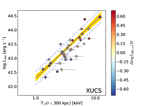
Figure 4: $L_{500}-T$ relation, color-coded by the offset from the mean $L_{X,ce}-M$ relation. The mean model and its 68% error are shown as a solid line and yellow shading, respectively. The mean model $\pm 1\sigma_{\text{intr}}$ is shown as dashed corridor. There is a tight scaling between $L_{500}$ and $T$, independent on cluster over/under luminosity (blue/red points are not systematically above or below the average), see also Fig. 5. Three clusters (observed by two telescopes) appear twice in the figure, but only the ones with smaller errors are used in the fit.

3.3 $L_{X}-T$

Fig. 4 shows the $L_{500}-T$ relation of XUCS clusters. To derive the fit parameters, we adopt Gaussian errors in $\log L_{500}$ and lognormal errors on $T_{X}$ and a Gaussian intrinsic scatter in $\log L_{500}|M$. Assuming weak priors and an uniform prior on $\log T$, we found

$$\log L_{500}=(2.02\pm 0.22)\log(T/3)+43.27\pm 0.05$$ (2)

where $T$ is in keV and $L_{500}$ is in erg s^-1 , with an intrinsic scatter of $0.23\pm 0.04$ dex and almost no covariance between parameters due to our choice of pivoting $T$ near the middle of the data distribution, 3 keV. The intrinsic scatter is much smaller than the range explored by the data (two dex, in the ordinate), unlike the mass-temperature relation were the intrinsic scatter is as large as allowed by the data scatter. An identical result is obtained by taking a Schechter (1976) prior mass converted in $T$ using the scaling relation in equation 1 inclusive of scatter, basically because the errors on $T$ are small compared to the prior width for almost all data points. This indicates that our results are independent of the shape of the $T$ distribution adopted for the sample.

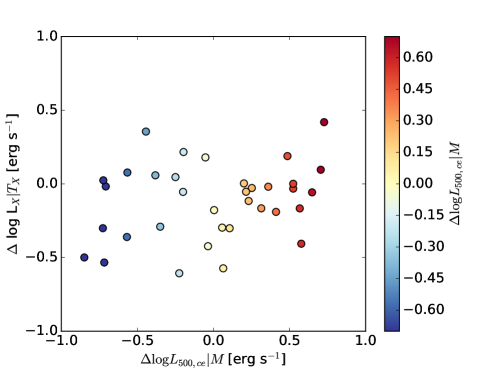
Figure 5: Residuals from the $L_{500}-T$ relation vs residuals from the $L_{500,ce}-M$ relation color-coded by offset from the mean $L_{X,ce}-M$ relation. Clusters faint/bright at a given mass are not systematically hot/cold. Three clusters (observed by two telescopes) appear twice in the figure.

Blue/red points are not systematically above, or below, the best fit. Therefore clusters have a temperature appropriate for their X-ray luminosity, regardless of their position on the $L_{X,ce}-M$ plane, i.e. of whether they are under/over luminous, of low/high surface brightness or with a small/large gas fraction. This can be better seen in Fig. 5 which shows the residuals from the $L_{500}-T$ and the $L_{500,ce}-M$ relations.

We interpret the tighter trend between $T$ and $L_{500}$ than $T$ and $M_{500}$ as due to the fact that X-ray luminosity and temperature are quantities dominated by photons coming from small radii (in particular for $T$ we used 300 kpc) and strongly affected by gas physics (e.g. shocks, cool-cores), while mass is dominated by dark matter at large radii: for example in a NFW profile with $c_{500}=5$ and $r_{500}=1$ Mpc, 70 % of the mass is at $r>300$ kpc. Thermodynamic properties at small radii are not much affected by the mass distribution at large radii, as even simple numerical experiments show, making temperature little affected by the amount of mass at large radii. Furthermore, during major, intermediate, and minor mergers, evolution moves simulated clusters in the $L_{X}-T$ plane mostly along the $L_{X}-T$ relation (e.g., Richter & Sarazin 2001; Poole et al. 2007). Therefore these events do not add scatter in the $L_{500}-T$ plane, while they might in the $L_{500}-M$ plane, for example, differences in mass accretion histories may contribute to the observed large scatter in the temperature-mass plane. To summarize, while in a simplified universe clusters are close to isothermal spheres in hydrostatic equilibrium with a scatter-less scaling between mass and temperature, the observed mass-temperature plot reminds us that what happens to the gas at small radii is not felt by dark matter at large radii and neither directly affected by it.

The analysis of deep follow-up data of one single X-ray faint cluster (Paper IV) already highlighted this detachment between local and global quantities, at least in that single object, and showed that this extends to other local/global quantities, such as central entropy and integrated pressure.

Fig. 4 suggests that clusters that are X-ray faint for their mass, or of low surface brightness within $r_{500}$, cannot be recognized in a $L_{500}-T$ diagram: they are not systematically offset from the mean relation, and therefore cannot be singled out in this kind of analysis. This indicates that the $L_{500}-T$ relation derived for X-ray selected samples is robust because the missed population (of low surface brightness) obeys the same $L_{500}-T$ of the detected population, as these analyses assume. Therefore, the lack of objects of low surface brightness in these samples does not introduce a (strong) bias in $L_{500}-T$ analyses. It will, instead, in $M-T$ analyses as obvious from Fig. 3.

4 Discussion

The $L_{500}-M$ relation derived for X-ray selected samples is biased high because cluster faint for their mass are underrepresented (Paper I). One may wonder if a similar bias might exist for the $L_{500}-T$ scaling as well. Our X-ray unbiased sample already indicates this is not the case because this scaling relation does not depend on the offset from the $L_{500,ce}-M$ scaling law (sec. 3). Nevertheless, a direct comparison with X-ray selected samples would be reassuring.

Fig. 6 shows the $L_{500}-T$ plot of the XXL-100 sample, color-coded by redshift, and corrected for evolution to the median redshift of the XUCS sample, $z=0.085$, according to the best fit evolution computed by Giles et al. (2016). The two points with $kT\sim 3$ keV and $\log L_{500}\sim 42.2$ erg s^-1 that stand out of the mean relation are likely to have measurement problems (Giles et al. 2016) and one of them had $kT=0.6^{+0.2}_{-0.1}$ in an earlier analysis (Pierre et al. 2006).

XXL-100 data points are in broad agreement with XUCS fit (Fig. 6). The Giles et al. (2016) XXL-100 best-fit relation (slope, intercept, and scatter) agrees with the one derived for XUCS within the errors. However, a later, very similar, analysis adopting similar assumptions for an enlarged sample by the same team (Adami et al. 2018) prefers a steeper slope inconsistent with XUCS one ($3.17\pm 0.16$ vs XUCS $2.02\pm 0.22$, about $4\sigma$ away, and XXL-100 $2.63\pm 0.15$). A closer look at the data and assumptions done to derive the best fit parameters is therefore in order.

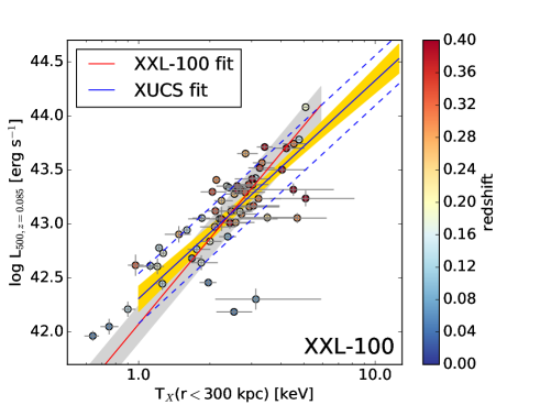
Figure 6: XXL-100 $L_{500}-T$ relation color-coded by redshift, corrected for evolution at the median redshift of XUCS. The two points with $\log L_{500}\sim 42.2$ and $T\sim 3$ kT, likely have problematic measurements (see Giles et al. 2016 and text). The red solied line is the best fit to the whole XXL-100 sample, while the gray shading marks the mean $\pm 1\sigma_{\text{intr}}$ corridor, as derived by Giles et al. (2016). The blue solid line, the yellow shading and the dashed lines mark the fit, uncertainty and $\pm 1\sigma_{\text{intr}}$ corridor of the XUCS sample. The two fits are consistent, although ours is derived with fewer assumptions and without the approximations assumed in XXL-100. Only $z<0.4$ XXL-100 clusters are shown, to focus on those with lower evolutionary corrections.

As most X-ray selected samples, larger values of X-ray luminosity are found at large redshifts because very bright clusters are rare and therefore are missing in the low volume of the local Universe. Since $T$ also increases with $L_{500}$, then the $L_{500}-T$ relation of X-ray selected samples displays a redshift gradient (see color coding in Fig. 6): clusters in the top-right of the $L_{500}-T$ diagram are the most distant ones, while those in the bottom-left corner are in the very nearby Universe. The effect would be more evident than seen in Fig. 6 also considering XXL-100 $z>0.4$ clusters because they all fall in the top-right part of the plot. Therefore, the $L_{500}-T$ slope and evolution are largely collinear (degenerate), i.e. the $L_{500}-T$ in such samples is equally well fitted by allowing larger slopes and smaller evolutions (as already reported for the $Y_{SZ}$ vs mass relation in Andreon 2014). Depending on the evolution parameter, the relation corrected for evolutionary effects rotates, and it does so hinged at the low-$L_{500}$ low-$T$ corner, since these clusters are in the nearby Universe and therefore are not affected by evolutionary corrections. Since XUCS clusters are instead all in a narrow redshift range, $\Delta z=0.085$, their differential evolution across the redshift range is negligible and the slope is not collinear with evolution. The collinearity explains the wide range of inferred slopes.

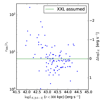
Figure 7: Assumed (green line) and observed (points) $r_{500}/r_{c}$ used by XXL-100 to compute the luminosity within $r_{500}$ from the luminosity within 300 kpc plotted in abscissa, and cluster detection probability. The right ordinates shows the luminosity offset for a cluster with $r_{500}=1$ Mpc on a logarithm scale. On average, the offset is $\pm 0.5$ dex, i.e. a factor of three. See text.

However, the collinearity does not explain why derived slopes are inconsistent, forcing us to look for sources of error underestimation that, if accounted for, would make measurements consistent. In their analysis, Giles et al. (2016) and Adam et al. (2018) make two assumptions, which are not included in their error budget. The first one is related to the missed population: basically, both works assume that missed clusters (those of low surface brightness) obey to the same $L_{500}-T$ scaling of the observed population, which our work shows for the first time to be close to be true. Second, as also noted by the authors, they assume that all clusters have $r_{c}=0.15r_{500}$ with no scatter. This assumption is made twice, both to extrapolate the X-ray luminosity within $r_{500}$ from the luminosity within the 300 kpc aperture assuming a beta-model, and to compute the detection probability. However, clusters are characterized by a wide scatter in $r_{500}/r_{c}$, as shown by Fig. 7 for the clusters in XXL-100. The left ordinate shows the ratio of published $r_{500}$ and $r_{c}$ values. The scatter between assumed and measured core radius is 0.27 dex (computed from the median absolute deviation to be tolerant to outliers), i.e. about a factor of 2. Figure 9 of Pacaud et al. (2016) shows that for clusters close to threshold of the bright sample studied by XXL-100, detectability is a strong function of the core radius and the sky coverage changes by more than a factor of 10 when $r_{c}$ is doubled. The right ordinate shows the ratio between the luminosity calculated assuming a fixed ratio $r_{500}/r_{c}$ as in XXL, and the actual luminosity using the $r_{c}$ from the fit with a $\beta$ model when $r_{500}=1$ Mpc. The scatter between the luminosity calculated with the two methods is $\Delta\log L_{500}=0.5$ dex (i.e. a factor of 3 brighter/fainter than correct).

Since Giles et al. (2016) and Adami et al. (2018) $L_{500}-T$ do not take these approximations into account in the error budget, the errors quoted are underestimated, resulting in an inconsistency between the three slope estimates. Since XUCS sample: a) is free from the slope-evolution degeneracy; b) does not miss clusters and therefore does not make hypotheses on the $L_{500}-T$ of the unseen population; c) does not assume a core radius to determine the cluster flux; - it can be used as reference and as a profitable prior for future analysis of X-ray samples to break the slope-evolutionary degeneracy.

Ge et al. (2019) also found similarity between the $L_{X}-T$ relations of optically- and X-ray selected samples. Their data however lack a reliable mass proxy not allowing them to, for example, address the $M-T$ relation, or to look for dependencies from the offset from the $L_{X}-M$ relation that our data allow. Based on the analysis of the XUCS sample, we suggest a different interpretation of the observed $L_{X}-T$ relation: while Ge et al. (2019) believe that low temperatures observed for rich clusters are due to failures of their adopted mass proxy, and that therefore they would disappear with proper mass proxy, our sample shows that mass is less directly related to temperature than temperature is to X-ray luminosity, and therefore that low temperatures are possible for clusters of large mass (and faint surface brightness) and this does not depend on a faulty measure of mass/richness.

5 Conclusions

In this work we analysed the mass-temperature and luminosity-temperature scaling relations of a sample that includes the recently discovered class of clusters that are X-ray faint for their mass, also known to have an average low surface brightness and a low gas fraction. We used a sample of 32 clusters in the nearby Universe selected independently of the intracluster medium properties, from which the first few examples were discovered in Paper I. Our sample can rely on mass measurement derived without dynamical or hydrostatic equilibrium hypothesis, with average error of 0.14 dex. Furthermore, our mass and temperature estimates are based on different and independent sets of data.

The sample was first presented in Andreon et al (2016). Here we use the same data to derive the temperature $T$ within a 300 kpc radius aperture, which we derive with a median error of 15%.

The main results of this work are that the $M_{500}-T$ relation has a large scatter, and the location of a cluster in this plane depends on the cluster surface brightness. The wider scatter around the $M-T$ relation was missed thus far due to two concurrent factors: it is reduced if the sample does not contain low surface brightness clusters, therefore covering a smaller area of the $M-T$ plane, as in X-ray or SZ selected samples commonly studied in literature. Second, the determination of radius $r_{500}$ and mass $M_{500}$ from the temperature, gas fraction, gas mass, or $Y_{X}$, as it is commonly done in X-ray studies, also artificially reduces the scatter. The independent estimates of mass and temperature and the presence of clusters of low surface brightness in the XUCS sample revealed the full range of the cluster population in the $M-T$ plane.

Clusters obey a tight $L_{500}-T$ scaling, independently of their brightness within the $r_{500}$ scale, making this diagram not useful to recognize clusters of low surface brightness. For this reason surveys that miss clusters of low surface brightness may infer unbiased estimates of the $L_{500}-T$ scaling parameters.

We interpret the tighter relation between $T$ and $L_{500}$ than between $T$ and $M_{500}$ as due to the fact that X-ray luminosity and temperature are more directly related to each other than with mass: these quantities are dominated by photons coming from small radii (in particular for $T$ we used 300 kpc) and strongly affected by gas thermodynamics (e.g. shocks, cool-cores), while mass is dominated by dark matter at large radii.

Since the XUCS sample is spread on a very narrow redshift interval over which evolutionary effects are negligible and its selection function does not depend on X-ray properties, our determination of the $L_{X}-T$ relation is free from the collinearity (degeneracy) between evolution and slope and free from hypothesis on the undetected population, both affecting current X-ray selected samples. We derive a slope of $L_{500}-T$ relation of $2.0\pm 0.2$. Because of the reduced number of assumptions, our determination can be used both as reference and to break the above degeneracy in X-ray selected samples.

Data Availability

All the values needed for reproduce the plots in this Paper concerning the XUCS sample are in Table 1 or were published in Paper I. Raw data are in the X-ray and SDSS archives. Data for the XXL-100 samples are published as detailed in the quoted references.

References

- [Adami et al.(2018)] Adami, C., Giles, P., Koulouridis, E., et al. 2018, A&A, 620, A5.
- [Aihara et al.(2018)] Aihara, H., Arimoto, N., Armstrong, R., et al. 2018, PASJ, 70, S4.
- [Andreon(2012)] Andreon, S. 2012, A&A, 546, A6.
- [Andreon(2014)] Andreon, S. 2014, A&A, 570, L10.
- [Andreon & Bergé(2012)] Andreon, S. & Bergé, J. 2012, A&A, 547, A117.
- [Andreon & Hurn(2013)] Andreon, S. & Hurn, M. 2013, Statistical Analysis and Data Mining: The ASA Data Science Journal, 9, 15.
- [Andreon & Moretti(2011)] Andreon, S., & Moretti, A. 2011, A&A, 536, A37
- [Andreon & Weaver(2015)] Andreon, S. & Weaver, B. 2015, Bayesian Methods for the Physical Sciences. Learning from Examples in Astronomy and Physics, by S. Andreon and B. Weaver. Springer Series in Astrostatistics, Vol. 4.
- [Andreon et al.(2011)] Andreon, S., Trinchieri, G., & Pizzolato, F. 2011, MNRAS, 412, 2391
- [Andreon et al.(2016)] Andreon, S., Serra, A. L., Moretti, A., et al. 2016, A&A, 585, A147 (Paper I).
- [Andreon et al.(2017a)] Andreon, S., Wang, J., Trinchieri, G., et al. 2017, A&A, 606, A24 (Paper II).
- [Andreon et al.(2017b)] Andreon, S., Trinchieri, G., Moretti, A., et al. 2017, A&A, 606, A25 (Paper III).
- [Andreon et al.(2019)] Andreon, S., Moretti, A., Trinchieri, G., et al. 2019, A&A, 630, A78 (Paper IV).
- [Andreon et al.(2021)] Andreon, S., Romero, C., Castagna, F., et al. 2021, MNRAS, 505, 5896.
- [Andreon et al.(2022)] Andreon, S. et al. 2022, in preparation
- [Arnaud(1996)] Arnaud, K. A. 1996, Astronomical Data Analysis Software and Systems V, 101, 17
- [Arnaud et al.(2010)] Arnaud, M., Pratt, G. W., Piffaretti, R., et al. 2010, A&A, 517, A92
- [Böhringer et al.(2007)] Böhringer, H., Schuecker, P., Pratt, G. W., et al. 2007, A&A, 469, 363.
- [Chen et al.(2019)] Chen, H., Avestruz, C., Kravtsov, A. V., et al. 2019, MNRAS, 490, 2380.
- [Chiu et al.(2021)] Chiu, I.-N., Ghirardini, V., Liu, A., et al. 2021, A&A, submitted (arXiv:2107.05652)
- [Diaferio & Geller(1997)] Diaferio, A. & Geller, M. J. 1997, ApJ, 481, 633.
- [Dickey & Lockman(1990)] Dickey, J. M. & Lockman, F. J. 1990, ARA&A, 28, 215.
- [Eckert et al.(2011)] Eckert, D., Molendi, S., & Paltani, S. 2011, A&A, 526, AA79
- [Fabjan et al.(2011)] Fabjan, D., Borgani, S., Rasia, E., et al. 2011, MNRAS, 416, 801.
- [Ge et al.(2019)] Ge, C., Sun, M., Rozo, E., et al. 2019, MNRAS, 484, 1946.
- [Geller et al.(2013)] Geller, M. J., Diaferio, A., Rines, K. J., et al. 2013, ApJ, 764, 58.
- [Giles et al.(2016)] Giles, P. A., Maughan, B. J., Pacaud, F., et al. 2016, A&A, 592, A3.
- [Hoekstra et al.(2015)] Hoekstra, H., Herbonnet, R., Muzzin, A., et al. 2015, MNRAS, 449, 685.
- [Kaiser(1986)] Kaiser, N. 1986, MNRAS, 222, 323.
- [Kravtsov et al.(2006)] Kravtsov, A. V., Vikhlinin, A., & Nagai, D. 2006, ApJ, 650, 128.
- [Lieu et al.(2016)] Lieu, M., Smith, G. P., Giles, P. A., et al. 2016, A&A, 592, A4.
- [Liu et al.(2021)] Liu, T., Buchner, J., Nandra, K., et al. 2022, A&A, submitted (arXiv:2106.14522)
- [Lovisari et al.(2020)] Lovisari, L., Schellenberger, G., Sereno, M., et al. 2020, ApJ, 892, 102.
- [Maughan et al.(2012)] Maughan, B. J., Giles, P. A., Randall, S. W., Jones, C., & Forman, W. R. 2012, MNRAS, 421, 1583
- [Maughan et al.(2016)] Maughan, B. J., Giles, P. A., Rines, K. J., et al. 2016, MNRAS, 461, 4182.
- [Mantz et al.(2010)] Mantz, A., Allen, S. W., Ebeling, H., et al. 2010, MNRAS, 406, 1773.
- [Moretti et al.(2009)] Moretti, A., Pagani, C., Cusumano, G., et al. 2009, A&A, 493, 501.
- [Nagai et al.(2007)] Nagai, D., Kravtsov, A. V., & Vikhlinin, A. 2007a, ApJ, 668, 1.
- [Nagai et al.(2007)] Nagai, D., Vikhlinin, A., & Kravtsov, A. V. 2007b, ApJ, 655, 98.
- [Navarro et al.(1997)] Navarro, J. F., Frenk, C. S., & White, S. D. M. 1997, ApJ, 490, 493.
- [Orlowski-Scherer et al.(2021)] Orlowski-Scherer, J., Di Mascolo, L., Bhandarkar, T., et al. 2021, A&A, 653, A135.
- [O’Sullivan et al.(2017)] O’Sullivan, E., Ponman, T. J., Kolokythas, K., et al. 2017, MNRAS, 472, 1482.
- [Pacaud et al.(2007)] Pacaud, F., Pierre, M., Adami, C., et al. 2007, MNRAS, 382, 1289
- [Pacaud et al.(2016)] Pacaud, F., Clerc, N., Giles, P. A., et al. 2016, A&A, 592, A2.
- [Pearson et al.(2017)] Pearson, R. J., Ponman, T. J., Norberg, P., et al. 2017, MNRAS, 469, 3489.
- [Pierre et al.(2006)] Pierre, M., Pacaud, F., Duc, P.-A., et al. 2006, MNRAS, 372, 591.
- [Pierre et al.(2016)] Pierre, M., Pacaud, F., Adami, C., et al. 2016, A&A, 592, A1.
- [Planck Collaboration et al.(2011)] Planck Collaboration, Aghanim, N., Arnaud, M., et al. 2011, A&A, 536, AA9
- [Planck Collaboration et al.(2012)] Planck Collaboration, Aghanim, N., Arnaud, M., et al. 2012, A&A, 543, AA102
- [Poole et al.(2007)] Poole, G. B., Babul, A., McCarthy, I. G., et al. 2007, MNRAS, 380, 437.
- [Ragagnin] Ragagnin, A., Andreon, S. 2022, A&A, in prep.
- [Ricker & Sarazin(2001)] Ricker, P. M. & Sarazin, C. L. 2001, ApJ, 561, 621.
- [Sarazin(1988)] Sarazin, C. L. 1988, Cambridge Astrophysics Series, Cambridge: Cambridge University Press, 1988
- [Schechter(1976)] Schechter, P. 1976, ApJ, 203, 297.
- [Smith et al.(2001)] Smith, R. K., Brickhouse, N. S., Liedahl, D. A., & Raymond, J. C. 2001, ApJ, 556, L91
- [Stanek et al.(2010)] Stanek, R., Rasia, E., Evrard, A. E., et al. 2010, ApJ, 715, 1508.
- [Umetsu et al.(2020)] Umetsu, K., Sereno, M., Lieu, M., et al. 2020, ApJ, 890, 148.
- [Vikhlinin et al.(2006)] Vikhlinin, A., Kravtsov, A., Forman, W., et al. 2006, ApJ, 640, 691.
- [Xu et al.(2018)] Xu, W., Ramos-Ceja, M. E., Pacaud, F., et al. 2018, A&A, 619, A162.
- [Yang et al.(2009)] Yang, H.-Y. K., Ricker, P. M., & Sutter, P. M. 2009, ApJ, 699, 315.
- [Zhang et al.(2006)] Zhang, Y.-Y., Böhringer, H., Finoguenov, A., et al. 2006, A&A, 456, 55.
- [Zhang et al.(2007)] Zhang, Y.-Y., Finoguenov, A., Böhringer, H., et al. 2007, A&A, 467, 437.