Bootstrapping Pions at Large $N$

Abstract

We revisit from a modern bootstrap perspective the longstanding problem of solving QCD in the large $N$ limit. We derive universal bounds on the effective field theory of massless pions by imposing the full set of positivity constraints that follow from $2\to 2$ scattering. Some features of our exclusion plots have intriguing connections with hadronic phenomenology. The exclusion boundary exhibits a sharp kink, raising the tantalizing scenario that large $N$ QCD may sit at this kink. We critically examine this possibility, developing in the process a partial analytic understanding of the geometry of the bounds.

1 Introduction

Solving large $N$ QCD is a longstanding open problem. It has been apparent since the seminal work of ’t Hooft tHooft:1973alw that the generalization of QCD to $N$ colors and fixed number of quarks should admit a string theory description, which becomes perturbative as $N~{}\to~{}\infty$. ’t Hooft’s prophecy has been fully realized (within the standard framework of critical superstring theory, no less) for the maximally supersymmetric cousin of QCD Maldacena:1997re ; Gubser:1998bc ; Witten:1998qj and several related models. But despite interesting attempts (see e.g. Polyakov:1997tj ; Polyakov:1998ju ), we seem still far from a concrete worldsheet description of ordinary large $N$ QCD.

From a spacetime perspective, the formulation of the problem has also been clear for decades. At $N~{}=~{}\infty$, the spectrum of QCD consists of infinite towers of stable color-singlet hadrons tHooft:1973alw ; Witten:1979kh ; to leading large $N$ order, hadronic scattering amplitudes are meromorphic functions that satisfy standard crossing and unitarity constraints and have well-understood high-energy limits.

Carving out the space of large $N$ gauge theories

It seems very natural to revisit this classic problem in the spirit of the modern bootstrap program. We have an infinite-dimensional set of observables (hadronic masses and spins, and their cubic on-shell couplings) obeying an infinite-dimensional set of constraints (crossing and unitarity for all possible four-point scattering amplitudes). We expect these bootstrap equations to admit many solutions, one for each consistent large $N$ confining gauge theory. While it is a priori unclear how to directly zoom in on the solution that corresponds to large $N$ QCD, we may simply proceed to carve out the space of consistent possibilities, a strategy that has proved enormously successful in the conformal bootstrap Rattazzi:2008pe ; Poland:2018epd ; Poland:2022qrs . Does large $N$ QCD sit at a special point of the exclusion boundary (as is serendipitously the case for the 3D Ising CFT El-Showk:2012cjh )? Could further physical input (e.g. suitable spectral assumptions) narrow down the set of possibilities to a small numerical island?

The idea of bootstrapping the hadronic S-matrix is of course an ancient one. It predated QCD and led, via the discovery of the Veneziano amplitude Veneziano:1968yb , to the development of string theory itself. The S-matrix bootstrap program (for general QFTs) has undergone a recent renaissance (see e.g. Paulos:2016fap ; Paulos:2016but ; Paulos:2017fhb ; He:2018uxa ; Cordova:2018uop ; Homrich:2019cbt ; Bercini:2019vme ; Cordova:2019lot ; Hebbar:2020ukp ; Guerrieri:2020kcs ; He:2021eqn , and Kruczenski:2022lot for an overview). Emulating the modern conformal bootstrap, these new developments emphasize the role of theory space and rely on powerful numerical optimization methods. These ideas have been applied to real-world QCD in Guerrieri:2018uew ; Guerrieri:2020bto , with very intriguing results. Large $N$ leads to a major conceptual simplification. While the analytic structure of the finite $N$ hadronic S-matrix is still far from understood, the analyticity properties at large $N$ are uncontroversial (see e.g. Veneziano:2017cks for a recent discussion). Any $2\to 2$ connected amplitude is expected to be a meromorphic function of the Mandelstam invariants, with obvious crossing and unitarity properties; the high energy Regge behavior is controlled by the pomeron trajectory for glueball scattering and by the rho trajectory for meson scattering.

In this paper, we further specialize to the mesons. At leading large $N$ order, they form a consistent subsector, as only other mesons appear as intermediate states in meson-meson scattering amplitudes. (In the language of string theory, we would be studying tree-level open string amplitudes.) We consider the chiral limit of vanishing quark masses. Assuming that the standard pattern of chiral symmetry breaking persists at large $N$, the lowest lying mesons are the massless “pions”, in the adjoint representation of the $SU(N_{f})$ flavor group. It would be straightforward to generalize our analysis to include a non-zero quark mass, but we are in fact hoping that if any analytic clues are to be found, they will show up in the zeroth order approximation to QCD, which is large $N$ in the chiral limit.

Effective field theory and positivity

There is a neat way to organize our bootstrap problem, using the language of effective field theory (EFT). We introduce a cut-off scale $M$, and divide the mesons into light states with masses smaller than $M$, and heavy states with masses larger than $M$. In principle, if we knew the full large $N$ theory, the EFT of the light states would arise by integrating out the heavy states at tree level. (Recall that meson three-point vertices scale as $1/\sqrt{N}$, so at leading large $N$ order we are always justified in using the tree-level approximation.) Instead, we decide to be agnostic about the heavy data (either than they satisfy the usual axioms) and to constrain the low-energy EFT by imposing its compatibility with “healthy” scattering of the light states. The computational complexity grows with the number of light states, so in the simplest setup, the only light states are the massless pions; the cut-off scale $M$ can then be identified with the mass of the first massive state that appears in pion-pion scattering – in QCD, this would be the rho vector meson. The next step is to include the rho among the light states, and so on.

It has long been appreciated that not anything goes in EFT. For an EFT to arise as the low-energy approximation of a unitary and causal quantum field theory, its Wilson coefficients must obey certain inequalities. These “positivity” bounds have a long history originating precisely in pion physics (see Martin1969 ; Pham:1985cr ; Ananthanarayan:1994hf ; Pennington:1994kc ; Comellas:1995hq ; Dita:1998mh for some early references) and have been the subject of intense study since their significance was emphasized in Adams:2006sv , see e.g. Manohar:2008tc ; Mateu:2008gv ; Nicolis:2009qm ; Baumann:2015nta ; Bellazzini:2015cra ; Bellazzini:2016xrt ; Cheung:2016yqr ; Bonifacio:2016wcb ; Cheung:2016wjt ; deRham:2017avq ; Bellazzini:2017fep ; deRham:2017zjm ; deRham:2017imi ; Hinterbichler:2017qyt ; Bonifacio:2017nnt ; Bellazzini:2017bkb ; Bonifacio:2018vzv ; deRham:2018qqo ; Zhang:2018shp ; Bellazzini:2018paj ; Bellazzini:2019xts ; Melville:2019wyy ; deRham:2019ctd ; Alberte:2019xfh ; Alberte:2019zhd ; Bi:2019phv ; Remmen:2019cyz ; Ye:2019oxx ; Herrero-Valea:2019hde ; Bellazzini:2020cot ; Tolley:2020gtv ; Caron-Huot:2020cmc ; Arkani-Hamed:2020blm ; Sinha:2020win ; Trott:2020ebl ; Wang:2020jxr ; Zhang:2020jyn ; Zhang:2021eeo ; Du:2021byy ; Davighi:2021osh ; Chowdhury:2021ynh ; Henriksson:2021ymi ; Bern:2021ppb ; Caron-Huot:2021rmr ; Li:2021lpe ; deRham:2022hpx ; Caron-Huot:2022ugt ; Henriksson:2022oeu . To get started, one must make canonical assumptions about the S-matrix (such as analyticity, crossing, boundedness and a positive partial wave decomposition), which are believed to encode the fundamental principles of unitarity and causality. (As we have already remarked, all requisite axioms are very clear in our large $N$ setup.) The basic strategy is then to write a (suitably subtracted) dispersion relation for the $2\to 2$ amplitude, which expresses low-energy parameters in terms of an unknown but positive UV spectral density. Remarkably, one finds two-sided bounds that enforce the standard Wilsonian power counting, with higher dimensional operators suppressed by the appropriate powers of the UV cut-off.

Given the venerable history in the application of positivity bounds to pion physics Martin1969 ; Pham:1985cr ; Ananthanarayan:1994hf ; Pennington:1994kc ; Comellas:1995hq ; Dita:1998mh ; Manohar:2008tc ; Mateu:2008gv ; Alvarez:2021kpq ; Guerrieri:2018uew ; Guerrieri:2020bto ; Bose:2020cod ; Bose:2020shm ; Zahed:2021fkp , it may come as a surprise that we have something new to say. In fact, the full set of inequalities for Wilson coefficients that follow from $2\to 2$ scattering have been derived only very recently Tolley:2020gtv ; Caron-Huot:2020cmc ; Arkani-Hamed:2020blm . A key insight of these papers is that low-energy crossing symmetry implies the existence of an infinite set of “null constraints” for the heavy data, which in turn can be used to optimize the numerical bounds for the low-energy parameters. These methods are ideally suited for our problem, because at large $N$ we can treat the EFT at tree level and hence derive rigorous bounds on the Wilson coefficients.

Results

After generalizing the approach of Tolley:2020gtv ; Caron-Huot:2020cmc to the kinematic setup of large $N$ pion-pion scattering, we obtain novel numerical bounds for the leading higher-dimensional operators of the chiral Lagrangian. Our bounds are new because they take into account the full set of null constraints, up to numerical convergence. Let us highlight in this introduction a couple of our key results, to be discussed at length in the main text.

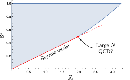
Figure 1: Exclusion plot in the space of four-derivative couplings. Healthy theories must lie inside the colored region.

We display in figure 1 the exclusion plot in the space of the two four-derivative couplings (normalized by the pion decay constant and in units of the UV cut-off $M$, see (51)). As expected, the allowed region is compact. Strikingly, the lower exclusion boundary displays a prominent kink. Unfortunately, we lack reliable data to place large $N$ QCD on this plot. There are a few lattice studies of mesons in large $N$ QCD (see e.g. Lucini:2012gg ; DeGrand:2016pur ; Hernandez:2019qed ; Perez:2020vbn ; Baeza-Ballesteros:2022azb ), but to the best of our knowledge the four-derivative Wilson coefficients have not been determined. The best we can currently do is to compare with real world, see figure 9. Apart from systematic errors due to finite $N$ (three of course) and the non-zero pion mass, experimental uncertainties are also quite large. Within these large errors real-world QCD is compatible with our bounds and perhaps prefers to sit near the lower boundary, but it seems challenging to draw any sharper conclusion. Curiously, the bottom part of the lower bound is a straight segment (shown in red in figure 1) whose slope agrees precisely with the choice made in the Skyrme model, i.e. with the combination of $O(p^{4})$ terms that has at most two time derivatives.

It is a well-known experimental fact (also confirmed by large $N$ lattice studies) that the lightest resonance in pion-pion scattering is the rho vector meson. If we make this spectral assumption, including the rho among the light states, the new cut-off $M^{\prime}$ is the mass of the next meson (in QCD, this is the $f_{2}(1270)$ state). This allows us to put an upper bound for the $g_{\pi\pi\rho}$ coupling, as shown in figure 2. Again, we see an interesting kink. We also find another curious connection with another bit of “voodoo QCD”. The value of $g_{\pi\pi\rho}$ at the plateau is rather close (but not equal) to the one that corresponds to the phenomenologically successful KSRF relation Kawarabayashi:1966kd ; Riazuddin:1966sw .

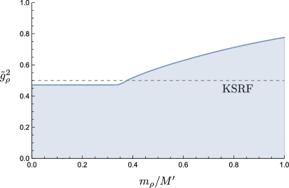
Figure 2: Upper bound on $g_{\pi\pi\rho}$ (normalized by $f_{\pi}$ and $m_{\rho}$, see (92)) as a function of the gap after the rho.

What is the physical significance of the kinks that we find in our plots? Do they correspond to large $N$ QCD (or, possibly, to some other interesting large $N$ gauge theory)? Following Caron-Huot:2020cmc , we are able to easily find simple extremal (unphysical) amplitudes that “explain” a large portion of the allowed region in figure 1, but leave out the most interesting part, a sliver where the kink sits. Several numerical experiments (playing with gaps and spectral assumptions) lead us to the hypothesis that two simple UV completions of the tree-level rho exchange amplitude might in fact explain the entire geometry of the bounds; the kink would arise because the two UV completions exchange dominance there. However we only succeeded in finding analytic expressions that rule in a part but not the entirety of the sliver, notably leaving out the kink, see figure 20. This may indicate a lack of imagination on our part, or that the physics of the kink is richer. We hasten to add that even if our hypothesis is correct (that there exist simple unphysical amplitudes sitting at the exclusion boundary in a two-dimensional projection of the full parameter space), this would not rule out that an actual physical theory such as QCD may saturate the same bounds.

The question of whether large $N$ QCD sits at the kink remains open. This paper is just a first step in a systematic program; we are optimistic to be able to address this and many other questions in future work.

The detailed organization of the paper is best apprehended from the table of contents. In section 2, we set up the problem, spelling out our analyticity, unitarity and Regge boundedness assumptions for pion scattering at large $N$. In section 3, we use dispersion relations to derive “positive” sum rules for the low-energy parameters in the pion EFT. In section 4 we use semidefinite programming methods to carve out the space of consistent low-energy parameters. We also compare our results with the previous literature and with the real world. In section 5, we include an explicit rho vector meson in the pion-pion amplitude, and derive bounds for the $g_{\pi\pi\rho}$ coupling. In section 6 we look for an analytic (or at least conceptual) understanding of the geometry of our bounds. We conclude in section 7 with a brief discussion and directions for future work. In appendix A we review the standard nomenclature for mesons and the selection rules that apply to pion-pion scattering at large $N$. In appendix B we give the generalization of our kinematic setup to a general number $N_{f}$ of fundamental quarks.

2 Setup and assumptions

Consider four-dimensional $SU(N)$ Yang-Mills theory with $N_{f}$ fundamental massless Dirac fermions, in the standard large $N$ ’t Hooft limit tHooft:1973alw . We will make the usual (uncontroversial) assumption that the theory remains confining at large $N$, so that that the asymptotic states are color-singlet glueballs, mesons and (heavy) baryons Witten:1979kh . Here we will be concerned with the mesons, and in particular with the scattering of the lowest-lying ones. We further assume the standard pattern of chiral symmetry breaking, so that the lightest mesons are the massless Goldstone bosons $\pi^{a}$ ($a=1,2,\ldots,N_{f}^{2}-1$), in the adjoint representation of $SU(N_{f})$. For $N_{f}=2$, this is the isospin triplet of pions and for $N_{f}=3$, the octet of pions, kaons and the eta. By a slight abuse of terminology, we will refer to them as pions regardless of $N_{f}$.

2.1 Parametrizations and crossing symmetry

In the $1/N$ expansion, quark loops and non-planar diagrams are down by powers of $1/N$, so at leading order only diagrams with the topology of a disk delimited by an external quark loop contribute to meson scattering tHooft:1973alw ; Witten:1979kh (see figure 3). The only dependence on the flavor indices of these diagrams comes as a single trace of the $SU(N_{f})$ generators. Therefore, at leading large $N$ order the scattering amplitude for the process $\pi^{a}\pi^{b}\to\pi^{c}\pi^{d}$ can be parametrized as

$${\cal T}_{ab}^{cd}=\, 4\left[\text{Tr}\left(T_{a}T_{b}T^{c}T^{d}\right)+\text{Tr}\left(T_{a}T^{d}T^{c}T_{b}\right)\right]M(s,t)$$

$$+\, 4\left[\text{Tr}\left(T_{a}T^{c}T^{d}T_{b}\right)+\text{Tr}\left(T_{a}T_{b}T^{d}T^{c}\right)\right]M(s,u)$$

$$+\, 4\left[\text{Tr}\left(T_{a}T^{d}T_{b}T^{c}\right)+\text{Tr}\left(T_{a}T^{c}T_{b}T^{d}\right)\right]M(t,u)\,.$$ (1)

Since we are scattering identical particles, the basic amplitude $M(s,u)$ enjoys $s\leftrightarrow u$ crossing symmetry, i.e.

$$M(s,u)=M(u,s)\,.$$ (2)

It does not, however, enjoy full $s\leftrightarrow t\leftrightarrow u$ crossing symmetry because the outer quark loop fixes the ordering of the external states. This parametrization is very natural in the language of tree-level string theory, where $M(s,u)$ is the basic disk amplitude (such as the Beta function in the case of the Veneziano amplitude) and the flavor structure is introduced via Chan-Paton factors. But at this stage, (2.1) is purely a kinematic statement.

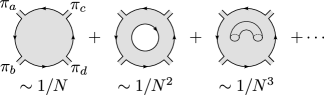
Figure 3: As $N\to\infty$ the diagrams contributing to $\pi\pi\to\pi\pi$ scattering arrange in a topological expansion in powers of $1/N$. At leading order, only planar diagrams with the topology of a disk survive. Quark loops are suppressed by $1/N$ and handles (which make the diagram non-planar) by $1/N^{2}$. Solid oriented lines denote quark propagators, the shaded area represents all possible (planar) dressings with gluons.

Although we will mostly use (2.1), another parametrization that will prove useful is

$${\cal T}_{ab}^{cd}\, =A(s|t,u)\left(\frac{2}{N_{f}}\delta_{ab}\delta^{cd}+d_{abe}d^{cde}\right)$$

$$\;+A(t|s,u)\left(\frac{2}{N_{f}}\delta_{a}^{d}\delta^{c}_{b}+d\indices{{}_{a}^{d}{}_{e}}d\indices{{}_{b}^{ce}}\right)$$

$$\;+A(u|s,t)\left(\frac{2}{N_{f}}\delta_{a}^{c}\delta^{d}_{b}+d\indices{{}_{a}^{c}{}_{e}}d\indices{{}^{d}_{b}{}^{e}}\right)\,.$$ (3)

Crossing symmetry is now the statement that

$$A(s|t,u)=A(s|u,t)\,.$$ (4)

Using

$$\text{Tr}\left(T_{a}T_{b}T^{c}T^{d}\right)+\text{Tr}\left(T_{a}T^{d}T^{c}T_{b}\right)= \;\frac{1}{2N_{f}}\left(\delta_{ab}\delta^{cd}+\delta_{a}^{d}\delta^{c}_{b}-\delta_{a}^{c}\delta^{d}_{b}\right)$$

$$+\;\frac{1}{4}\left(d_{abe}d^{cde}+d\indices{{}_{a}^{d}{}_{e}}d\indices{{}_{b}^{ce}}-d\indices{{}_{a}^{c}{}_{e}}d\indices{{}^{d}_{b}{}^{e}}\right)\,,$$ (5)

we see that the two parametrizations are related by

$$A(s|t,u)=M(s,t)+M(s,u)-M(t,u)\,,\quad 2M(s,u)=A(s|t,u)+A(u|s,t)\,.$$ (6)

The $\boldsymbol{\eta^{\prime}}$ meson

A subtlety of the large $N$ expansion is that the axial anomaly is suppressed in this limit (see e.g. Witten:1979vv ; Veneziano:1979ec ; Leutwyler:1997yr ; Kaiser:2000gs ). The axial $U(1)$ is then non-anomalous at $N=\infty$ and its spontaneous breaking brings in a new Goldstone boson; the —now massless— $\eta^{\prime}$ meson. More precisely, the pattern of chiral symmetry breaking gets upgraded from $SU(N_{f})_{\text{L}}\times SU(N_{f})_{\text{R}}\times U(1)_{\text{V}}\to U(N_{f})_{\text{V}}$ to $U(N_{f})_{\text{L}}\times U(N_{f})_{\text{R}}\to U(N_{f})_{\text{V}}$, so the $\eta^{\prime}$ meson becomes degenerate with the pions forming a multiplet of $U(N_{f})$. For this reason, to incorporate the $\eta^{\prime}$ in pion scattering we just have to consider the additional generator $T_{0}=\frac{1}{\sqrt{2N_{f}}}\mathbb{1}$, associated to the determinant of the matrices in $U(N_{f})$, for any leg involving an $\eta^{\prime}$. Thus, scattering processes between pions and the $\eta^{\prime}$ can be described with the same basic amplitudes as above. Indeed, defining the fully $s\leftrightarrow t\leftrightarrow u$ symmetric amplitude

$$A_{stu}\equiv A(s|t,u)+A(t|s,u)+A(u|s,t)=M(s,t)+M(s,u)+M(t,u)\,,$$ (7)

we have respectively for the processes $2\eta^{\prime}\to 2\eta^{\prime}$, $2\eta^{\prime}\to\eta^{\prime}\pi$, $2\eta^{\prime}\to 2\pi$, $\eta^{\prime}\pi\to 2\pi$, the amplitudes

$${\cal T}_{00}^{00}=\frac{2}{N_{f}}A_{stu}\,,\quad{\cal T}_{00}^{0d}=0\,,\quad{\cal T}_{00}^{cd}=\frac{2}{N_{f}}A_{stu}\delta^{cd}\,,\quad{\cal T}_{0b}^{cd}=\sqrt{\frac{2}{N_{f}}}A_{stu}d\indices{{}_{b}^{cd}}\,.$$ (8)

Since including the $\eta^{\prime}$ does not bring any additional information, we will only consider the scattering of $SU(N_{f})$ pions from this point forward.

2.2 Analyticity and Zweig’s rule

We can further rewrite the amplitude ${\cal T}_{ab}^{cd}$ as a sum over the $SU(N_{f})$ irreducible representations (irreps) that can appear as intermediate states. For the sake of clarity, we restrict to $N_{f}=2$ for the following discussion, but our conclusions will actually apply to any $N_{f}$. The derivation for general $N_{f}$ is given in appendix B. The $2\to 2$ scattering of $SU(2)$ pions splits into three isospin channels, ${\mathcal{I}}=1\otimes 1=0\oplus 1\oplus 2$. So we can rewrite the amplitude as

$${\cal T}=\sum_{{\mathcal{I}}=0}^{2}\mathcal{M}^{{\mathcal{I}}}(s|t,u)\mathbb{P}^{{\mathcal{I}}}_{s}\,,$$ (9)

where $\mathbb{P}^{{\mathcal{I}}}_{s}$ are the $s$-channel isospin projectors

$$\mathbb{P}^{0}_{s}=\frac{1}{3}\delta_{ab}\delta^{cd}\,,\quad\mathbb{P}^{1}_{s}=\frac{1}{2}\left(\delta_{a}^{c}\delta_{b}^{d}-\delta_{a}^{d}\delta_{b}^{c}\right)\,,\quad\mathbb{P}^{2}_{s}=\frac{1}{2}\left(\delta_{a}^{c}\delta_{b}^{d}+\delta_{a}^{d}\delta_{b}^{c}-\frac{2}{3}\delta_{ab}\delta^{cd}\right)\,,$$ (10)

and the amplitudes in the different channels are related to the previous parametrizations by

$$\mathcal{M}^{0}(s|t,u)=\; 3A(s|t,u)+A(t|s,u)+A(u|s,t)=3M(s,t)+3M(s,u)-M(t,u)\,,$$ (11a)

$$\mathcal{M}^{1}(s|t,u)=\; A(u|s,t)-A(t|s,u)=2\Big{(}M(s,u)-M(s,t)\Big{)}\,,$$ (11b)

$$\mathcal{M}^{2}(s|t,u)=\; A(t|s,u)+A(u|s,t)=2M(t,u)\,.$$ (11c)

Note that under $t\leftrightarrow u$ crossing $\mathcal{M}^{{\mathcal{I}}}(s|t,u)$ is symmetric for ${\mathcal{I}}=0,2$ and antisymmetric for ${\mathcal{I}}=1$. Under $s\leftrightarrow t$ crossing they mix into one another.

At leading order in $1/N$, the pion scattering amplitude reduces to an infinite sum of tree diagrams corresponding to the exchange of physical mesons Witten:1979kh . Thus, for fixed $u<0$, $M(s,u)$ is a meromorphic function with poles on the real $s$ axis. Also at $N=\infty$, mesons are exactly $q\bar{q}$ states, i.e. there are no exotic mesons. Since massless quarks have isospin ${\mathcal{I}}=\frac{1}{2}$, this implies that the physical intermediate states in large $N$ pion scattering can only carry two possible representations; ${\mathcal{I}}=\frac{1}{2}\otimes\frac{1}{2}=0\oplus 1$.

Diagrams contributing to the ${\mathcal{I}}=2$ channel either come from the exchange of exotic mesons or are such that the initial and final states can be separated by cutting only internal gluon lines. The former cannot happen at large $N$, and the latter are processes suppressed by Zweig’s rule, which becomes exact in the limit $N\to\infty$. In the language of string theory, these two types of process correspond respectively to exchanging multiple open strings or exchanging a closed string and are therefore down by powers of the string coupling constant. Of course, this should only be taken as a picture, we are emphatically not making any dynamical assumption that the theory must be a theory of strings – we are just imposing large $N$ selection rules.

In summary, the isospin-two amplitude cannot have physical poles at large $N$. In other words,  $\mathcal{M}^{2}(s|t,u)$ for fixed $u<0$ must be analytic on the real $s>0$ axis. From (11c) we conclude that $M(s,u)$ (for fixed $u<0$) only has poles on the positive real $s$ axis, i.e. it does not have $t$-channel poles. Indeed, a pole at negative $s$ would correspond to a pole for positive $t$ which would contribute a physical state in the partial wave expansion of $\mathcal{M}^{2}(s|t,u)$.

2.3 Unitarity

Each $\mathcal{M}^{{\mathcal{I}}}(s|t,u)$ admits an s-channel partial wave expansion,

$$\mathcal{M}^{{\mathcal{I}}}(s|t,u)=s^{\frac{4-D}{2}}\sum_{J}n^{(D)}_{J}c^{({\mathcal{I}})}_{J}(s)\mathcal{P}_{J}\left(1+\frac{2u}{s}\right)\,,$$ (13)

where the normalization constant is chosen as

$$n_{J}^{(D)}\equiv\frac{2^{D}\pi^{\frac{D-2}{2}}}{\Gamma(\tfrac{D-2}{2})}(J+1)_{D-4}(2J+D-3)\,,$$ (14)

so that the Gegenbauer polynomials are defined by

$$\mathcal{P}_{J}(x)\equiv{}_{2}F_{1}\left(-J,J+D-3,\frac{D-2}{2},\frac{1-x}{2}\right)\,.$$ (15)

With these normalizations, unitarity for the amplitude $\mathcal{M}^{{\mathcal{I}}}(s|t,u)$ implies $|1+ic^{({\mathcal{I}})}_{J}(s)|^{2}\leq 1$ in the physical regime $s>0$. Defining the spectral densities $\rho^{({\mathcal{I}})}_{J}(s)={\rm Im}\,c^{({\mathcal{I}})}_{J}(s)$, this condition translates into

$$2\geq\rho^{({\mathcal{I}})}_{J}(s)\geq 0\,,\qquad s>0\,.$$ (16)

For the full amplitude ${\cal T}_{ab}^{cd}$ to define a unitary $S$-matrix, we need each of the isospin amplitudes (11) to be separately unitary. As discussed above, the ${\mathcal{I}}=2$ amplitude is analytic in the physical region, hence $\rho^{(2)}_{J}(s)=0$ for $s>0$ (at leading order in large $N$). Using the identity $\mathcal{P}_{J}(-x)=(-1)^{J}\mathcal{P}_{J}(x)$ and the symmetry properties of (11) under $t\leftrightarrow u$ crossing, we see that $\rho^{(0)}_{J}(s)$ is only nonvanishing for $J$ even and $\rho^{(1)}_{J}(s)$ for $J$ odd. Thus, if we expand the basic amplitude $M(s,u)$ as

$${\rm Im}\,M(s,u)=s^{\frac{4-D}{2}}\sum_{J}n^{(D)}_{J}\rho_{J}(s)\,\mathcal{P}_{J}\left({1+\frac{2u}{s}}\right)\,,$$ (17)

with

$$\rho_{J}(s) = \frac{1}{6}\rho^{(0)}_{J}(s)\qquad s>0\,,\;J\;{\rm even}\,,$$ (18a)

$$\rho_{J}(s) = \frac{1}{4}\rho^{(1)}_{J}(s)\qquad s>0\,,\;J\;{\rm odd}\,,$$ (18b)

unitarity of the full scattering amplitude implies positivity of $M(s,u)$. That is,

$$\rho_{J}(s)\geq 0\,,\qquad s>0\,,\;\text{all }J\,.$$ (19)

For a meromorphic function, the only contribution to the spectral density comes from the isolated poles, which give delta functions,

$$M(s,u)\sim g_{\pi\pi\alpha}^{2}\frac{m_{\alpha}^{2}\mathcal{P}_{J}\left(1+\frac{2u}{s}\right)}{m_{\alpha}^{2}-s}\,,\quad\longrightarrow\quad n_{J}^{(D)}\rho_{J}(s)\sim\pi\,g_{\pi\pi\alpha}^{2}\delta(s-m_{\alpha}^{2})\,m_{\alpha}^{D-2}\,.$$ (20)

Then, (19) implies the positivity of the coupling constants squared, $g_{\pi\pi\alpha}^{2}\geq 0$. We will not use the upper bounds on $g_{\pi\pi\alpha}^{2}$ coming from (16) because meson interactions scale as $g_{\pi\pi\alpha}\sim 1/\sqrt{N}$ and thus die at large $N$. (This is precisely what allows us to treat the meson theory at tree level in the first place.) The positivity condition will be enough. However, we will mostly use it in the form of (19) because we will parametrize our ignorance of the meson spectrum by a whole cut on the real $s$ axis rather than isolated poles.

2.4 Regge behavior

At finite $N$, pion scattering is believed to have Regge behavior controlled by the pomeron trajectory, which needs to have intercept above one to account for the rise with energy of the total cross section, see e.g. the discussion in Brower:2006ea . The pomeron trajectory corresponds to glueball states and is suppressed at large $N$. In string theory language, the pomeron is a closed string trajectory, and contributes to an open string amplitude via a subleading (non-planar) topology. The dominant trajectories after the pomeron are the rho trajectory and the $P^{\prime}$ trajectory (associated to the $f_{2}$(1270) resonance). In the analysis of appendix B of Pelaez:2004vs these two trajectories are taken to have the same intercept, $\alpha_{\rho}(0)=\alpha_{P^{\prime}}(0)\cong 0.52$. So to leading order in $N$ it seems safe to assume that the Regge behavior of ${\cal T}_{ab}^{cd}$ is strictly better than spin one. This translates into two conditions on $M(s,u)$,

$$\lim_{|s|\to\infty}\frac{M(s,u)}{s}=0\,,\quad\lim_{|s|\to\infty}\frac{M(s,-s-u)}{s}=0\,,\quad u\lesssim 0\,.$$ (21)

They are respectively the limits at fixed $u$ and at fixed $t$ of $M(s,u)$, which are independent when the amplitude is not fully crossing symmetric.

We will study these amplitudes around $u\sim 0$. For the first amplitude in (21) this corresponds to the usual forward limit $\cos\theta\sim 1$, for the second one, this is the “backward limit” $\cos\theta\sim-1$. It would be very interesting to study scattering at fixed angle $\theta$ (away from $0$ and $\pi$) since this could discern between standard string amplitudes, which decay exponentially at high energies, and amplitudes in QCD-like theories, which are expected to decay as $1/s^{2}$ by the Brodsky-Farrar counting rules Brodsky:1973kr ; Lepage:1980fj . Also at fixed angle, albeit in the unphysical regime $s,u\gg 1$, scattering amplitudes of large-$N$ confining gauge theories are known to follow a universal behavior Caron-Huot:2016icg . Unfortunately, fixed-angle scattering amplitudes fall outside the scope of our methods.

2.5 An example: The Lovelace-Shapiro amplitude

A remarkable function that obeys all of our assumptions for $M(s,u)$ at large $N$ is the Lovelace-Shapiro amplitude Lovelace:1968kjy ; Shapiro:1969km (see Bianchi:2020cfc for a recent discussion),

$$M_{\rm LS}(s,u)=-\frac{\Gamma(1/2-\alpha^{\prime}s)\Gamma(1/2-\alpha^{\prime}u)}{\Gamma(-\alpha^{\prime}(s+u))}\,.$$ (22)

For fixed $u$, this amplitude has poles only for positive $s$, with a positive-definite partial wave expansion. As discussed, this ensures that it does not have physical poles in the ${\mathcal{I}}=2$ channel. Note also the Adler zero $M_{\rm LS}(s,u)\sim\pi\alpha^{\prime}(s+u)$ for $s,u\to 0$, which agrees with the fact that Goldstone bosons have derivative couplings.

3 Sum rules from dispersion relations

The Regge behavior (21) implies that for fixed $u<0$, all the isospin amplitudes $\mathcal{M}^{{\mathcal{I}}}(s|t,u)$ grow more slowly than $\sim s$ at infinity. Thus, we can obtain three sets of $k$-subtracted dispersion relations by taking contour integrals in $s$ around infinity for each of these amplitudes,

$$\frac{1}{2\pi i}\oint_{\infty}ds^{\prime}\,\frac{\mathcal{M}^{{\mathcal{I}}}(s^{\prime}|-s^{\prime}-u,u)}{s^{\prime k+1}}=0\,,\quad k=1,2,\dots\,,\;{\mathcal{I}}=0,1,2\,.$$ (23)

By (11), these relations can be traded for the following dispersion relations of the basic amplitude $M(s,u)$,

$$\frac{1}{2\pi i}\oint_{\infty}ds^{\prime}\,\frac{M(s^{\prime},u)}{s^{\prime k+1}}=\frac{1}{2\pi i}\oint_{\infty}ds^{\prime}\,\frac{M(-s^{\prime}-u,u)}{s^{\prime k+1}}=\frac{1}{2\pi i}\oint_{\infty}ds^{\prime}\,\frac{M(s^{\prime},-s^{\prime}-u)}{s^{\prime k+1}}=0\,.$$ (24)

For $N_{f}>2$, instead of the three isospin channels we should consider all the channels discussed in appendix B, but that does not bring in additional constraints since all the amplitudes can be written in terms of the three crossed versions of $M(s,u)$ (see (139)). The three sets from (24) are all we need independently from the number of flavors. In fact, we only need the first and last one of them. Under the change of variables $s^{\prime}\to-s^{\prime}-u$, the second set of dispersion relations in (24) reduces to the first one (albeit with the subtraction shifted from 0 to $-u$) and it is thus redundant.

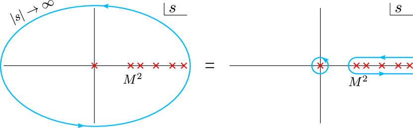
(a) SU dispersion relations.

(b) ST dispersion relations.

Figure 4: Contour deformations for the two independent sets of dispersion relations. The high-energy poles correspond to the meson spectrum.

As discussed above, $M(s,u)$ has physical poles in $s$ and $u$ (related by crossing symmetry) but not in $t$. Thus, for fixed $u<0$, $M(s,u)$ only has poles on the positive side of the real $s$ axis while $M(s,-s-u)$ has poles on both sides. Using that the amplitude is analytic away from the real $s$ axis, we can safely deform the contours towards the real axis as shown in figure 4. We will separate low and high energies by a cutoff scale $M^{2}$ such that all the poles lie above the cutoff and $M(s,u)$ is analytic below it. One should think of $M^{2}$ as the mass of the first exchanged meson in the spectrum. Then, with the contour deformations of figure 4, the two sets of independent dispersion relations relate low and high energies by

$$\text{SU:}\quad\frac{1}{2\pi i}\oint_{0}ds^{\prime}\,\frac{M_{\text{low}}(s^{\prime},u)}{s^{\prime k+1}}=\frac{1}{\pi}\int_{M^{2}}^{\infty}ds^{\prime}\frac{\text{Im}\,M_{\rm high}(s^{\prime},u)}{s^{\prime k+1}}\,,\qquad k=1,2,\dots$$ (25a)

$$\text{ST:}\quad\frac{1}{2\pi i}\oint_{0}ds^{\prime}\,\frac{M_{\text{low}}(s^{\prime},-s^{\prime}-u)}{s^{\prime k+1}} =\frac{1}{\pi}\int_{M^{2}}^{\infty}ds^{\prime}\frac{\text{Im}\,M_{\rm high}(s^{\prime},-s^{\prime}-u)}{s^{\prime k+1}}\quad\qquad k=1,2,\dots\,$$

$$+\frac{1}{\pi}\int_{M^{2}}^{\infty}ds^{\prime}(-1)^{k}\frac{\text{Im}\,M_{\rm high}(s^{\prime},-s^{\prime}-u)}{(s^{\prime}+u)^{k+1}}\,,$$ (25b)

where we have used that the discontinuity of $M(s,u)$ is equal to its imaginary part, $\text{Im}\,M(s,u)=\frac{1}{2i}\left[M(s+i\epsilon,u)-M(s-i\epsilon,u)\right]$. These two independent sets of dispersion relations are in essence “fixed $u$” and “fixed $t$” dispersion relations. There are two of them because the amplitude is $s\leftrightarrow u$ crossing symmetric. For a fully $s\leftrightarrow t\leftrightarrow u$ symmetric theory, both sets would be equivalent.

3.1 Low energy: Effective field theory

As usual, we describe the physics at low energy with an effective field theory (EFT). The standard EFT for pion scattering is the chiral Lagrangian Gasser:1983yg ; Gasser:1984gg . The spontaneously broken chiral symmetry determines the $n$-point vertices, $n>4$, in terms of the 4-point interactions (with arbitrarily many derivatives), but since we are only studying pion $2\to 2$ scattering, we will be blind to this fact. The only input about the Goldstone boson nature of the pions that we can try to impose (apart that they are massless) is that they are derivatively coupled, but in fact the need to perform at least one substraction means that the quartic non-derivative coupling drops out from our sum rules.

Like any other EFT, the chiral Lagrangian comprises all the terms that are consistent with the symmetries of the theory, but with unfixed coefficients. If we knew the full underlying theory, we could compute these coefficients by integrating out the higher mesons in the spectrum, but since that is not the case, the coefficients must be fixed differently. The usual way of doing so is by comparison to experiment or from lattice computations. Our approach will be to bootstrap them, i.e. we will ask what values of these coefficients are compatible with an underlying theory satisfying the assumptions of section 2.

Instead of using the EFT Lagrangian, which is defined up to field redefinitions and integration by parts, we define the low-energy coefficients directly at the level of the amplitude, which is unambiguous. We defer the relation to the chiral Lagrangian to section 4.4. At the level of the amplitude, integrating out the heavy mesons leaves a series of four-point interaction vertices as in figure 5. Thus, for energies below the cutoff we can describe $M(s,u)$ by

$${M}_{\rm low}(s,u) = \sum_{n=1}^{\infty}\sum_{\ell=0}^{[n/2]}g_{n,\ell}\,(s^{n-\ell}u^{\ell}+u^{n-\ell}s^{\ell})$$

$$= g_{1,0}(s+u)+g_{2,0}(s^{2}+u^{2})+2g_{2,1}\,su+g_{3,0}(s^{3}+u^{3})+g_{3,1}(s^{2}u+u^{2}s)+\dots\,,$$

where $g_{n,\ell}$ are the low energy coefficients that we will bound. They represent the (unknown) coupling constants of the four-point vertices of figure 5. Equation (3.1) is essentially the crossing-symmetric Taylor expansion of the full amplitude $M(s,u)$ around $s\sim u\sim 0$, which converges as long we do not step on any singularity, i.e. at energies below $M^{2}$. Note also that (3.1) incorporates the Adler zero ($M(s,u)\to 0$ as $s,u\to 0$), as befits the derivative couplings of Goldstone bosons.

Figure 5: The EFT amplitude for $2\to 2$ pion scattering is given by an infinite sum of four-point vertices with unknown coefficients. The sum can be arranged into a series with increasing number of derivatives in the interaction.

3.2 High energy: Partial wave unitarity

On the other hand, we will be agnostic about the physics above the cutoff. Even though we know that $M(s,u)$ becomes meromorphic in the $N\to\infty$ limit, we do not know the position of the poles or their coupling constants. Therefore, at high energies we will expand $M(s,u)$ in partial waves as in (17),

$${\rm Im}\,M_{\text{high}}(s,u)=s^{\frac{4-D}{2}}\sum_{J}n^{(D)}_{J}\rho_{J}(s)\,\mathcal{P}_{J}\left({1+\frac{2u}{s}}\right)\,,$$ (27)

with a general spectral density $\rho_{J}(s)$ that can have support anywhere on $s\geq M^{2}$. In other words, we are effectively allowing for a cut on the real $s$ axis rather than a collection of poles – this is not unlike the conformal bootstrap, where one does not a priori input discreteness of the operator spectrum. The only assumption we will make about the theory at high energies is that it remains unitary, and in particular that the spectral density satisfies the lower bound $\rho_{J}(s)\geq 0$.

It is convenient to define the high-energy averages

$$\Big{\langle}(\cdots)\Big{\rangle}\equiv\frac{1}{\pi}\sum_{J}n^{(D)}_{J}\int_{M^{2}}^{\infty}\frac{dm^{2}}{m^{2}}m^{4-D}\rho_{J}(m^{2})\;(\cdots)\,,$$ (28)

which have positive measure by the assumption of unitarity at high energies. Plugging (27) into (25) and using $\mathcal{P}_{J}(-x)=(-1)^{J}\mathcal{P}_{J}(x)$ together with crossing symmetry then gives the sum rules

$$\text{SU:}\quad\frac{1}{2\pi i}\oint_{0}ds^{\prime}\,\frac{M_{\text{low}}(s^{\prime},u)}{s^{\prime k+1}}=\Big{\langle}\frac{\mathcal{P}_{J}(1+\frac{2u}{m^{2}})}{m^{2k}}\Big{\rangle}\,,\qquad k=1,2,\dots$$ (29a)

$$\text{ST:}\quad\frac{1}{2\pi i}\oint_{0}ds^{\prime}\,\frac{M_{\text{low}}(s^{\prime},-s^{\prime}-u)}{s^{\prime k+1}} =\Big{\langle}\frac{(-1)^{J}\mathcal{P}_{J}(1+\frac{2u}{m^{2}})}{m^{2k}}\Big{\rangle}\qquad k=1,2,\dots\,$$ (29b)

$$+ \,\Big{\langle}(-1)^{k}\frac{m^{2}(-1)^{J}\,\mathcal{P}_{J}(1+\frac{2u}{m^{2}})}{(m^{2}+u)^{k+1}}\Big{\rangle}\,.$$

Let us stress again that although we have in mind large $N$ pion scattering, these sum rules are more general, and so will be our results. Since we are not using that the amplitude is actually meromorphic, these sum rules apply to any $s\leftrightarrow u$ crossing-symmetric unitary amplitude $M(s,u)$ satisfying the Regge behavior (21) and such that at fixed $u<0$ it is analytic away from the positive real $s$ axis. This last condition is perhaps the strongest, expressing a clear feature (the Zweig rule) of large $N$ kinematics.

3.3 SU sum rules

We have managed to relate the low-energy pole to an average on the high-energy states. Now we just have to plug (3.1) into the left hand side of (29), expand the right hand side around $u\sim 0$ (the forward limit) and match the coefficients to obtain separate sum rules for the couplings $g_{n,\ell}$. The first few SU sum rules read:

$$k=1\,: \quad g_{1,0}+2g_{2,1}u+g_{3,1}u^{2}+\cdots =\Big{\langle}\frac{\mathcal{P}_{J}(1)}{m^{2}}+2\frac{\mathcal{P}_{J}^{(1)}(1)}{m^{4}}u+2\frac{\mathcal{P}_{J}^{(2)}(1)}{m^{6}}u^{2}+\cdots\Big{\rangle}$$ (30a)

$$k=2\,: \quad g_{2,0}+g_{3,1}u+2g_{4,2}u^{2}+\dots =\Big{\langle}\frac{\mathcal{P}_{J}(1)}{m^{4}}+2\frac{\mathcal{P}_{J}^{(1)}(1)}{m^{6}}u+2\frac{\mathcal{P}_{J}^{(2)}(1)}{m^{8}}u^{2}+\cdots\Big{\rangle}$$ (30b)

$$k=3\,: \quad g_{3,0}+g_{4,1}u+g_{5,2}u^{2}+\dots =\Big{\langle}\frac{\mathcal{P}_{J}(1)}{m^{6}}+2\frac{\mathcal{P}_{J}^{(1)}(1)}{m^{8}}u+2\frac{\mathcal{P}_{J}^{(2)}(1)}{m^{10}}u^{2}+\cdots\Big{\rangle}\,.$$ (30c)

Note that changing the number of subtractions $k$ allows us to pick different powers of $s$ in the expansion of $M_{\text{low}}(s,u)$. The general expression for the $k$-subtracted SU sum rule is

$$\sum_{\ell=0}^{k}g_{k+\ell,\ell}\,u^{\ell}+\sum_{n=2k}^{\infty}g_{n,k}\,u^{n-k}=\sum_{i=0}^{\infty}\frac{2^{i}}{i!}\Big{\langle}\frac{\mathcal{P}_{J}^{(i)}(1)}{m^{2(k+i)}}\Big{\rangle}\,u^{i}\,,\quad k=1,2,\dots\,,$$ (31)

where we have used the linearity of the high-energy average (28).

The couplings $g_{k,0}$ and $g_{2k,k}$ appear only in the $k$-subtracted sum rule. By matching the coefficients of the Taylor expansion in $u$, we find

$$g_{k,0}=\Big{\langle}\frac{1}{m^{2k}}\Big{\rangle}\,,\qquad g_{2k,k}=\frac{2^{k-1}}{k!}\Big{\langle}\frac{\mathcal{P}_{J}^{(k)}(1)}{m^{4k}}\Big{\rangle}\,,\quad k=1,2,\dots\,.$$ (32a)

Meanwhile, all the other couplings $$g_{n,\ell} \ell\neq 0 n\neq 2\ell k=\ell k=n-\ell$$ (with and ) appear precisely in two sum rules (namely the ones with and ) giving rise to two distinct expressions in terms of high-energy averages,

$$g_{n,\ell}=\frac{2^{n-\ell}}{(n-\ell)!}\Big{\langle}\frac{\mathcal{P}_{J}^{(n-\ell)}(1)}{m^{2n}}\Big{\rangle}=\frac{2^{\ell}}{\ell!}\Big{\langle}\frac{\mathcal{P}_{J}^{(\ell)}(1)}{m^{2n}}\Big{\rangle}\,,\qquad\begin{aligned} n&=3,4,\dots\,\\ \ell&=1,\dots,\left[\tfrac{n-1}{2}\right]\,.\end{aligned}$$ (32b)

Imposing equality of the two expressions gives rise to an infinite set of null constraints

$${\cal X}_{n,\ell}(m^{2},J)\equiv\frac{2^{n-\ell}}{(n-\ell)!}\frac{\mathcal{P}_{J}^{(n-\ell)}(1)}{m^{2n}}-\frac{2^{\ell}}{\ell!}\frac{\mathcal{P}_{J}^{(\ell)}(1)}{m^{2n}}\,,\qquad\begin{aligned} n&=3,4,\dots\,\\ \ell&=1,\dots,\left[\tfrac{n-1}{2}\right]\,,\end{aligned}$$ (33)

whose high-energy average must vanish,

$$\Big{\langle}{\cal X}_{n,\ell}(m^{2},J)\Big{\rangle}=0\,.$$ (34)

This imposes highly nontrivial constraints on the heavy data; not anything goes for a unitary UV-complete theory.

3.4 ST sum rules

Following the same procedure for the ST sum rules, we reach the general expression for the $k$-subtracted sum rule,

$$\sum_{n=k}^{\infty} \sum_{\ell=0}^{[n/2]}g_{n,\ell}\left((-1)^{\ell}\frac{\left(k-(n-\ell)+1\right)_{n-k}}{(n-k)!}+(-1)^{n-\ell}\frac{\left(k-\ell+1\right)_{n-k}}{(n-k)!}\right)u^{n-k}\qquad k=1,2,\dots$$

$$=\sum_{i=0}^{\infty}\left(\frac{2^{i}}{i!}\Big{\langle}\frac{(-1)^{J}\mathcal{P}_{J}^{(i)}(1)}{m^{2(k+i)}}\Big{\rangle}\,u^{i}+\sum_{j=0}^{\infty}(-1)^{k+j}\frac{(j+1)_{k}}{k!}\frac{2^{i}}{i!}\Big{\langle}\frac{(-1)^{J}\mathcal{P}_{J}^{(i)}(1)}{m^{2(k+i+j)}}\Big{\rangle}u^{i+j}\right)\,,$$ (35)

where $(x)_{n}\equiv\Gamma(x+n)/\Gamma(n)$ is the Pochhammer symbol. Equating the coefficients of $u^{n-k}$ for fixed $n\geq k$,

$$\sum_{\ell=0}^{[n/2]} g_{n,\ell}\left((-1)^{\ell}\frac{\left(k-(n-\ell)+1\right)_{n-k}}{(n-k)!}+(-1)^{n-\ell}\frac{\left(k-\ell+1\right)_{n-k}}{(n-k)!}\right)\quad\qquad k=1,2,\dots,n$$

$$=\frac{2^{n-k}}{(n-k)!}\Big{\langle}\frac{(-1)^{J}\mathcal{P}_{J}^{(n-k)}(1)}{m^{2n}}\Big{\rangle}+\sum_{i=0}^{n-k}(-1)^{n-i}\frac{(n-k-i+1)_{k}}{k!}\frac{2^{i}}{i!}\Big{\langle}\frac{(-1)^{J}\mathcal{P}_{J}^{(i)}(1)}{m^{2n}}\Big{\rangle}\,.$$ (36)

As (32) already gives us a sum rule for every coupling $g_{n,\ell}$, there is no need to solve for them here. Instead, we can use those sum rules to get rid of the couplings and derive a new infinite set of null constraints. It would look like at each level $n$ one gets $n$ new null constraints, but not all of them are independent. One can check that the first equations with $k=1,\ldots,\left[\tfrac{n}{2}\right]$ suffice. Plugging (32) into the left hand side of these equations yields the second set of null constraints:

$$\bigg{<}\mathcal{Y}_{n,k}(m^{2},J)\bigg{>}=0\;,$$ (37)

where

$$\mathcal{Y}_{n,k}(m^{2},J)= \sum_{\ell=0}^{k}(-1)^{n-\ell}\frac{\left(k-\ell+1\right)_{n-k}}{(n-k)!}\frac{2^{\ell}}{\ell!}\frac{\mathcal{P}_{J}^{(\ell)}(1)}{m^{2n}}-\frac{2^{n-k}}{(n-k)!}\frac{(-1)^{J}\mathcal{P}_{J}^{(n-k)}(1)}{m^{2n}}$$

$$- \sum_{i=0}^{n-k}(-1)^{n-i}\frac{(n-k-i+1)_{k}}{k!}\frac{2^{i}}{i!}\frac{(-1)^{J}\mathcal{P}_{J}^{(i)}(1)}{m^{2n}}\,,\qquad\begin{aligned} n&=2,3,\dots\,\\ k&=1,\dots,\left[\tfrac{n}{2}\right]\,.\end{aligned}$$ (38)

Recalling from (33) that the null constraints $\mathcal{X}_{n,\ell}$ exist for $\ell=1,\ldots,\left[\tfrac{n-1}{2}\right]$, we conclude that at a given level $n\geq 2$ there are

$$\bigg{[}\frac{n}{2}\bigg{]}+\left[\frac{n-1}{2}\right]=n-1\text{ null constraints.}$$ (39)

The first few null constraints are (in arbitrary normalization)

$$m^{4}\mathcal{Y}_{2,1} =\left(1-(-1)^{J}\right)(2-D)+\mathcal{J}^{2}\;,$$

$$m^{6}\mathcal{Y}_{3,1} =3\left(1-(-1)^{J}\right)(2-D)+2\left(1-2(-1)^{J}\right)\mathcal{J}^{2}\;,$$

$$m^{6}\mathcal{X}_{3,1} =2(1-D)\mathcal{J}^{2}+\mathcal{J}^{4}\;,$$

$$m^{8}\mathcal{Y}_{4,1} =2\left(1-(-1)^{J}\right)(2-D)D+\left(4(-1)^{J}+D\left(1-5(-1)^{J}\right)\right)\mathcal{J}^{2}+2(-1)^{J}\mathcal{J}^{4}\;,$$

$$m^{8}\mathcal{X}_{4,1} =\left(8-18D+D^{2}\right)\mathcal{J}^{2}+(8-6D)\mathcal{J}^{4}+2\mathcal{J}^{6}\;,$$

$$m^{8}\mathcal{Y}_{4,2} =-3\left(1-(-1)^{J}\right)D+\left(1-2(-1)^{J}\right)\mathcal{J}^{2}\;,$$ (40)

where ${\mathcal{J}}^{2}\equiv J\left(J+D-3\right)$ is the quadratic Casimir of the little group $SO\left(D-1\right)$. Note that all of them vanish for $J=0$, implying that spinless heavy states are decoupled from the states with $J\geq 1$. This was expected, as we only used dispersion relations with at least one subtraction due to the Regge behavior (21).

3.5 A second look at the high-energy behavior

Now we can ask if it would make sense to make boundedness assumptions stronger than (21). For example, if we assumed that the amplitude died asymptotically in the forward limit, i.e.

$$\lim_{|s|\to\infty}M(s,u)=0\,,\qquad u\lesssim 0\,,$$ (41)

we could write down unsubtracted SU dispersion relations. This means that (25a) would also hold for $k=0$. Following the same steps as above, this would yield —among others— the sum rule

$$g_{0,0}=\Big{\langle}1\Big{\rangle}\,,$$ (42)

where $g_{0,0}$ is the would-be constant term in (3.1). Since pion scattering amplitudes must satisfy the Adler zero $M(0,0)=0$, we must have $g_{0,0}=0$. But then the sum rule (42) cannot be satisfied by any non-trivial theory due to the positivity of the high-energy average $\left<\cdots\right>$. This contradiction proves that (41) is too strong an assumption; one should stick to the milder Regge behavior of (21).

4 Positivity bounds

It has long been known that dispersion relations link low and high energies in such a way that allows us to bound EFT couplings as a consequence of unitarity at high energies Martin1969 ; Pham:1985cr ; Ananthanarayan:1994hf ; Pennington:1994kc ; Comellas:1995hq ; Dita:1998mh . But only recently (building on much previous work, e.g. Adams:2006sv ; Manohar:2008tc ; Mateu:2008gv ; Nicolis:2009qm ; Baumann:2015nta ; Bellazzini:2015cra ; Bellazzini:2016xrt ; Cheung:2016yqr ; Bonifacio:2016wcb ; Cheung:2016wjt ; deRham:2017avq ; Bellazzini:2017fep ; deRham:2017zjm ; deRham:2017imi ; Hinterbichler:2017qyt ; Bonifacio:2017nnt ; Bellazzini:2017bkb ; Bonifacio:2018vzv ; deRham:2018qqo ; Zhang:2018shp ; Bellazzini:2018paj ; Bellazzini:2019xts ; Melville:2019wyy ; deRham:2019ctd ; Alberte:2019xfh ; Alberte:2019zhd ; Bi:2019phv ; Remmen:2019cyz ; Ye:2019oxx ; Herrero-Valea:2019hde ; Bellazzini:2020cot ) the full set of inequalities that follow from $2\to 2$ scattering have been derived Caron-Huot:2020cmc ; Tolley:2020gtv , exploiting the role of null constraints. Here we will use the method introduced in Caron-Huot:2020cmc to obtain optimal two-sided bounds on normalized ratios of the EFT coefficients $g_{n,\ell}$ using semidefinite programming. We start with a brief review of their approach using a slight reformulation that draws an analogy with the familiar conformal bootstrap. This will prove useful for the modifications that we will introduce in section 5. Then we present our results and we compare them to meson phenomenology and to previous work.

4.1 Dual problem

In the previous section we have expressed the dispersion relations (24) in terms of sum rules and null constraints of the form

$$g_{n,\ell}= \,\Big{\langle}g_{n,\ell}\left(m^{2},J\right)\Big{\rangle}\,,$$

$$0= \,\Big{\langle}{\mathcal{X}}_{n,\ell}\left(m^{2},J\right)\Big{\rangle}\,,\quad 0=\Big{\langle}{\mathcal{Y}}_{n,\ell}\left(m^{2},J\right)\Big{\rangle}\,,$$ (43)

where $\left<\cdots\right>$ denotes the high-energy average introduced in (28), which integrates —with positive measure— over all masses $m$ above the cutoff scale $M$ and sums over all spins $J=0,1,2\ldots$. The goal is to use these ingredients to obtain two-sided bounds for any given coupling $g_{n,\ell}$ normalized by $g_{1,0}$ and the cutoff as

$$\tilde{g}_{n,\ell}=g_{n,\ell}\frac{M^{2(n-1)}}{g_{1,0}}\,.$$ (44)

To do so, we define the vectors

$$\vec{v}_{\mathbb{1}}=\begin{pmatrix}1\\ 0\\ 0\\ \vdots\\ 0\end{pmatrix}\,,\qquad\vec{v}_{\mathcal{O}}=\begin{pmatrix}0\\ 1\\ 0\\ \vdots\\ 0\end{pmatrix}\,,\qquad\vec{v}_{\text{HE}}\left(m^{2},J\right)=\begin{pmatrix}-g_{1,0}\left(m^{2},J\right)M^{2}\\ -g_{n,\ell}\left(m^{2},J\right)M^{2n}\\ \mathcal{Y}_{2,1}\left(m^{2},J\right)M^{4}\\ \mathcal{X}_{3,1}\left(m^{2},J\right)M^{6}\\ \vdots\end{pmatrix}\,,$$ (45)

where the last vector includes as many null constraints as we like.

These vectors clearly satisfy the equation

$$g_{1,0}\,M^{2}\,\vec{v}_{\mathbb{1}}+g_{n,\ell}\,M^{2n}\,\vec{v}_{\mathcal{O}}+\Big{\langle}\vec{v}_{\text{HE}}\left(m^{2},J\right)\Big{\rangle}=0\,.$$ (46)

This is to be understood as a bootstrap equation analogous to that of the conformal bootstrap where $\vec{v}_{\mathbb{1}}$ plays the role of the identity operator, $\vec{v}_{\mathcal{O}}$ corresponds to an operator we are singling out and $\vec{v}_{\text{HE}}\left(m^{2},J\right)$ represents a continuum of heavy operators. With these identifications, we see that the low-energy coefficients are analogous to the OPE coefficients squared and the positivity of $\left<\cdots\right>$ corresponds to the statement of unitarity for the heavy operators. Obtaining bounds for the low-energy couplings is thus as easy as bounding OPE coefficients in the conformal bootstrap Caracciolo:2009bx :

We must look for a “functional” $\vec{\alpha}$ such that

1. is normalized as $\vec{\alpha}\cdot\vec{v}_{\mathcal{O}}=\left\{\begin{matrix}+1\quad\text{for upper bound}\\ -1\quad\text{for lower bound,}\end{matrix}\right.$

2. is positive on all heavy states, $\vec{\alpha}\cdot\vec{v}_{\text{HE}}\left(m^{2},J\right)\geq 0\quad\forall J,\,m\geq M$,

3. and maximizes $\vec{\alpha}\cdot\vec{v}_{\mathbb{1}}$.

Once we find such a functional, the positivity of the high-energy average guarantees that

$$\Big{\langle}\vec{\alpha}\cdot\vec{v}_{\text{HE}}\left(m^{2},J\right)\Big{\rangle}\geq 0\,.$$ (47)

So, by contracting (46) with $\vec{\alpha}$ and using the linearity of $\left<\cdots\right>$ we can get the bounds

$$\vec{\alpha}_{(-)}\cdot\vec{v}_{\mathbb{1}}\leq\tilde{g}_{n,\ell}\leq-\left(\vec{\alpha}_{(+)}\cdot\vec{v}_{\mathbb{1}}\right)\,,$$ (48)

where the subscript denotes the choice of normalization for the functional. The maximization condition on the functional makes the bounds as strong as possible.

This can be formulated as a semidefinite problem and solved for example with SDPB sdpb . When implementing it numerically, though, one must deal with infinities. The three infinities in the problem are the masses of the high-energy vectors, their spins and the number of available null constraints. As a semidefinite problem solver, SDPB imposes positivity on polynomials for $x\geq 0$, so replacing $m^{2}\to M^{2}\left(1+x\right)$ and removing the common denominator in $v_{\text{HE}}\left(m^{2},J\right)$ readily allows us to cover all the region $m^{2}\in\left[M^{2},\infty\right)$. As far as the spins go, we truncate the infinity by considering $J=0,1,2,\ldots,J_{\text{max}}$ with $J_{\text{max}}$ large enough that further increases of it do not change the results. By numerical experimentation we have seen that convergence in spins depends significantly more on how large $J_{\text{max}}$ is rather than on the density of the grid of spins. One can safely skip many intermediate spins so long as both even and odd spins are included.

The last infinity comes from the number of null constraints. Ideally, one would like to use all the null constraints derived in the previous section, but in practice one must truncate that infinity to construct finite-length vectors. We will consider vectors including all the null constraints up to “Mandelstam order” $n$, i.e. all the null constraints that follow from the terms in $M_{\text{low}}(s,u)$ up to order $O(p^{2n})$,

$${\mathcal{Y}}_{2,1},\;{\mathcal{Y}}_{3,1},\;{\mathcal{X}}_{3,1},\;{\mathcal{Y}}_{4,1},\;{\mathcal{X}}_{4,1},\;{\mathcal{Y}}_{4,2},\;\cdots\;{\mathcal{X}}_{n,\left[\frac{n-1}{2}\right]},\;{\mathcal{Y}}_{n,\left[\frac{n}{2}\right]}\,.$$

Up to a given order $n$, the total number of null constraints used is then

$$\sum_{i=2}^{n}\left(i-1\right)=\frac{1}{2}n\left(n-1\right)\,.$$ (49)

This makes $n$ analogous to the parameter $\Lambda$ that controls the number of derivatives of conformal blocks used in constructing the vectors for the conformal bootstrap. Just like in that case, increasing $n$ can only improve the bounds.

The above procedure can be used to bound any low-energy coupling, but in the following sections we will mostly be concerned with the first ones. The sum rules we will need are

$$g_{1,0}=\Big{\langle}\frac{1}{m^{2}}\Big{\rangle}\,,\qquad g_{2,0}=\Big{\langle}\frac{1}{m^{4}}\Big{\rangle}\,,\qquad g_{2,1}=\frac{1}{(D-2)}\Big{\langle}\frac{{\mathcal{J}}^{2}}{m^{4}}\Big{\rangle}\,,$$ (50)

where ${\mathcal{J}}^{2}\equiv J\left(J+D-3\right)$. Also, while we will keep our notation general, we set $D=4$ henceforth to make contact with the real world. For ease of notation, we define

$$\tilde{g}_{2}\equiv g_{2,0}\frac{M^{2}}{g_{1,0}}\,,\qquad\tilde{g}_{2}^{\prime}\equiv 2g_{2,1}\frac{M^{2}}{g_{1,0}}\,.$$ (51)

Note that it is safe to normalize by $g_{1,0}$ because the positivity of the high-energy average in (50) ensures that $g_{1,0}>0$ for any nontrivial theory. Using all the null constraints up to Mandelstam order $n=17$ (136 null constraints) we obtain the two-sided bounds

$$0\leq\tilde{g}_{2}\leq 1\,,\qquad 0\leq\tilde{g}_{2}^{\prime}\leq 3.25889135348...\,.$$ (52)

The lower bounds for these couplings are already obvious from the positivity of their sum rules, and so is the upper bound $\tilde{g}_{2}\leq 1$ if we recall that $m^{2}\geq M^{2}$ in the high-energy averages. The upper bound on $\tilde{g}_{2}^{\prime}$, on the other hand, is non-trivial.

4.2 Exclusion plot

Following again Caron-Huot:2020cmc , we can modify this program to place bounds on $\tilde{g}_{2}^{\prime}$ for every value of $\tilde{g}_{2}$ in its allowed range and thus carve out the space of EFTs that are compatible with unitary UV completions. Consider now the vectors

$$\vec{v}_{\mathbb{1}}=\begin{pmatrix}1\\ 0\\ 0\\ \vdots\\ 0\end{pmatrix}\,,\quad\vec{v}_{2}=\begin{pmatrix}0\\ 1\\ 0\\ \vdots\\ 0\end{pmatrix}\,,\quad\vec{v}_{2^{\prime}}=\begin{pmatrix}0\\ 0\\ 1\\ \vdots\\ 0\end{pmatrix}\,,\quad\vec{v}_{\text{HE}}\left(m^{2},J\right)=\begin{pmatrix}-M^{2}/m^{2}\\ -M^{4}/m^{4}\\ -\frac{2}{D-2}{\mathcal{J}}^{2}M^{4}/m^{4}\\ \mathcal{Y}_{2,1}\left(m^{2},J\right)M^{4}\\ \vdots\end{pmatrix}\,,$$ (53)

satisfying

$$\vec{v}_{\mathbb{1}}+\tilde{g}_{2}\,\vec{v}_{2}+\tilde{g}_{2}^{\prime}\,\vec{v}_{2^{\prime}}+\Big{\langle}\vec{v}_{\text{HE}}\left(m^{2},J\right)\Big{\rangle}=0\,.$$ (54)

For any fixed $\tilde{g}_{2}^{(0)}$, we can look for a functional $\vec{\alpha}$ that

1. is normalized as $\vec{\alpha}\cdot\vec{v}_{2^{\prime}}=\left\{\begin{matrix}+1\quad\text{for upper bound}\\ -1\quad\text{for lower bound,}\end{matrix}\right.$

2. is positive on all heavy states, $\vec{\alpha}\cdot\vec{v}_{\text{HE}}\left(m^{2},J\right)\geq 0\quad\forall J,\,m\geq M$,

3. and maximizes $\vec{\alpha}\cdot\left(\vec{v}_{\mathbb{1}}+\tilde{g}_{2}^{(0)}\vec{v}_{2}\right)$,

to get the bounds

$$\vec{\alpha}_{(-)}\cdot\left(\vec{v}_{\mathbb{1}}+\tilde{g}_{2}^{(0)}\vec{v}_{2}\right)\leq\tilde{g}_{2}^{\prime}\leq-\vec{\alpha}_{(+)}\cdot\left(\vec{v}_{\mathbb{1}}+\tilde{g}_{2}^{(0)}\vec{v}_{2}\right)\,.$$ (55)

Repeating these steps for several values of $\tilde{g}_{2}$ spanning its allowed range then yields the exclusion plot of allowed theories in the space of couplings $\left(\tilde{g}_{2}^{\prime},\tilde{g}_{2}\right)$, shown in figure 6.

Figure 6: Exclusion plots in the space of couplings $(\tilde{g}^{\prime}_{2},\tilde{g}_{2})$ for $D=4$ including all the null constraints up to Mandelstam order $n=2,3,7,11,15$. The colored area is the allowed region in each case. By $n=15$ the plot has visually converged and it shows three corners (labelled TL, TR, BL) and a kink (K).

The figure shows the exclusion plots obtained at different Mandelstam orders, each of them lying inside the previous one, as expected. Although the convergence in $n$ is somewhat slow, around $n=15$ the change becomes imperceptible. The final plot has a trapezoidal shape with three corners and a kink! At the top-right corner (TR), the value of $\tilde{g}_{2}^{\prime}$ matches its upper bound (52). This and the other two corners (top-left TL and bottom-left BL) can be understood in close analogy to Caron-Huot:2020cmc , as we explain in section 6. What is more intriguing is the kink (K). The optimistic hope is that it corresponds to large $N$ QCD in the chiral limit, but of course this does not have to be the case.

4.3 The kink

The lower part of the right-hand bound of figure 6, extending from the origin (BL) to the kink (K), corresponds to the line $\tilde{g}_{2}^{\prime}=4\,\tilde{g}_{2}$ for any $n$, and the kink moves down this line as we increase $n$. This bound appears already at order $n=2$, where we only use the null constraint ${\mathcal{Y}}_{2,1}$. Indeed, in this case the optimization problem tells us to look for a functional of the form $\vec{\alpha}=\left(\alpha_{1},\,\alpha_{2},\,1,\,\alpha_{4}\right)$ satisfying

$$\vec{\alpha}\cdot\vec{v}_{\text{HE}}\left(m^{2},J\right)=-\alpha_{1}\frac{M^{2}}{m^{2}}-\alpha_{2}\frac{M^{4}}{m^{4}}-{\mathcal{J}}^{2}\frac{M^{4}}{m^{4}}+\alpha_{4}\Big{(}2\left(1-(-1)^{J}\right)-\mathcal{J}^{2}\Big{)}\frac{M^{4}}{m^{4}}\geq 0\,,$$ (56)

for all $J$ and $m\geq M$, that maximizes $\alpha_{1}+\alpha_{2}\,\tilde{g}_{2}^{(0)}$. The solution to this problem is given by

$$\vec{\alpha}=\big{(}0,\,-4,\,1,\,-1\big{)}$$ (57)

for any value of $\tilde{g}_{2}^{(0)}$, resulting in the bound $\tilde{g}_{2}^{\prime}\leq 4\tilde{g}_{2}$. When further null constraints are included, there is a competition between solutions. For small enough $\tilde{g}_{2}^{(0)}$ this solution is still optimal, but as $\tilde{g}_{2}^{(0)}$ crosses a particular point (the kink), the minimization is suddenly achieved by a functional with nonzero $\alpha_{1}$ and lower $\alpha_{2}$. This is essentially a first order phase transition, in contrast to the case of Caron-Huot:2020cmc (see also Chiang:2021ziz ), where the transition looks second order with the discontinuity in the second derivative.

Knowing that the kink sits on top of the line $\tilde{g}_{2}^{\prime}=4\,\tilde{g}_{2}$, we can determine its precise position by looking for the upper bound on $\tilde{g}_{2}$ when a theory is forced to live on this line. This can be achieved by including as an additional null constraint the combination

$$\tilde{g}_{2}^{\prime}-4\,\tilde{g}_{2}\propto\Big{\langle}g_{2,1}\left(m^{2},J\right)M^{4}-2g_{2,0}\left(m^{2},J\right)M^{4}\Big{\rangle}=0\,.$$ (58)

Figure 7 shows the position of the kink computed in this way for increasing values of $n$. Its convergence is somewhat slow and, surprisingly, in steps of two. This indicates that the null constraints that contribute the most in shaping the plot are ${\mathcal{X}}_{n,\frac{n-1}{2}}$ (for odd $n$). From the first points in the plot it might seem that the kink is converging towards the exact value $0.5$, which would call for a simple analytic explanation, but at order $n=15$ we obtain

$$\tilde{g}_{2}^{(\text{K})}\simeq 0.4940\,,\qquad\tilde{g}_{2}^{\prime(\text{K})}=4\tilde{g}_{2}^{(\text{K})}\simeq 1.9760\,,\qquad(n=15)\,.$$ (59)

This already rules out the value $0.5$ and, in fact, the fit in figure 7 suggests that it converges to a value significantly lower; around $\tilde{g}_{2}^{(\text{K})}\sim 0.42$.

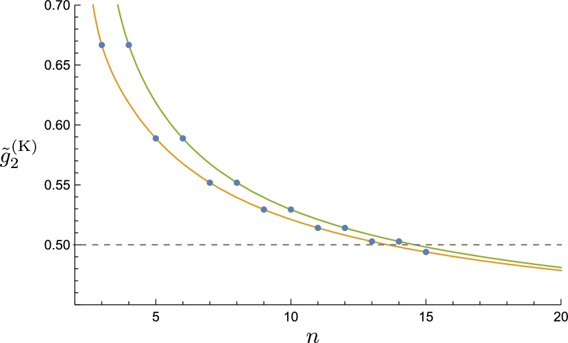
$n$	$\tilde{g}_{2}^{\text{(K)}}$
3, 4	0.6667
5, 6	0.5888
7, 8	0.5518
9, 10	0.5294
11, 12	0.5141
13, 14	0.5028
15	0.4940

Figure 7: Position of the kink along the $\tilde{g}_{2}^{\prime}=4\,\tilde{g}_{2}$ line as a function of the Mandelstam order $n$. The orange and green curves are, respectively, fits for the points of odd and even $n$ made with the function $f(n)=\sum_{i=0}^{5}\frac{a_{i}}{n^{i}}$ using the first six values in each case. The fits predict very well the last number in the table for $n=15$ ($n=16$ in the even $n$ case) and they suggest the asymptotic value $a_{0}\sim 0.42$.

Finally, to try to get a better picture of the kink, we have also solved the dual problem in a three-dimensional space using the coupling

$$\tilde{g}_{3}\equiv g_{3,0}\frac{M^{4}}{g_{1,0}}\,.$$ (60)

The results are shown in figure 8, where we have included two views of the 3D plot. The blue sheet represents the lower bound on $\tilde{g}_{3}$, while the orange sheet corresponds to its upper bound. From the picture on the left, we see that the allowed space at the plane $\tilde{g}_{2}^{\prime}=0$ is given by the convex hull of a parabola (that we will shortly identify) connecting the corners BL and TL along the blue sheet. The other view shows that the theories along the bound $\tilde{g}_{2}^{\prime}=4\,\tilde{g}_{2}$ also lie in the convex hull of a parabola, this one running from BL up to the kink K, at which point the blue and orange sheets fuse together.

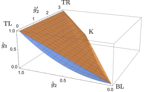
(a)

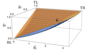
(b)

Figure 8: Two different views of the three-dimensional exclusion plot in the space $(\tilde{g}^{\prime}_{2},\tilde{g}_{2},\tilde{g}_{3})$. The blue sheet describes the lower bound on $\tilde{g}_{3}$ for every value of $\tilde{g}_{2}$ and $\tilde{g}_{2}^{\prime}$, the orange sheet is for the upper bound. This exclusion plot was made using all null constraints up to $n=7$.

4.4 QCD, where art thou?

We have obtained sharp bounds for the low energy couplings of EFTs for pion scattering. The question now is how do they compare to known EFTs? and more importantly, where is large $N$ QCD?

4.4.1 The chiral Lagrangian

As mentioned above, the EFT for pion scattering is the standard chiral Lagrangian (see e.g. Gasser:1983yg ; Gasser:1984gg ). The first terms of the $SU(N_{f})$ chiral Lagrangian for vanishing quark mass read

$$\mathcal{L}_{\text{Ch}}= -\frac{f_{\pi}^{2}}{4}\text{Tr}\left(\partial_{\mu}U^{\dagger}\partial^{\mu}U\right)+L_{1}^{\prime}\left[\text{Tr}\left(\partial_{\mu}U^{\dagger}\partial^{\mu}U\right)\right]^{2}+L_{2}^{\prime}\text{Tr}\left(\partial_{\mu}U^{\dagger}\partial_{\nu}U\right)\text{Tr}\left(\partial^{\mu}U^{\dagger}\partial^{\nu}U\right)$$

$$+L_{3}^{\prime}\text{Tr}\left(\partial_{\mu}U^{\dagger}\partial^{\mu}U\partial_{\nu}U^{\dagger}\partial^{\nu}U\right)+L_{4}^{\prime}\text{Tr}\left(\partial_{\mu}U^{\dagger}\partial_{\nu}U\partial^{\mu}U^{\dagger}\partial^{\nu}U\right)+\cdots\,,$$ (61)

where $U(x)=\exp\left[i\frac{2}{f_{\pi}}T_{a}\pi^{a}(x)\right]\in SU(N_{f})$ with $T_{a}$ the $SU(N_{f})$ generators in the defining representation. The coefficients $L_{i}^{\prime}$ are the low energy couplings that we alluded to before. They are in correspondence with the $g_{n,\ell}$ couplings in (3.1) and we will give their precise relation momentarily. Equation (4.4.1) includes all the independent chiral-invariant terms with four derivatives that we need for general $N_{f}$, but there are two special cases. For $N_{f}=3$, there is an identity that relates the last term to the other three four-derivative terms, so the $L_{4}^{\prime}$ term is dropped and the couplings are conventionally Gasser:1984gg renamed as

$$L_{1}^{\prime}\to L_{1}\equiv L_{1}^{\prime}+\frac{L_{4}^{\prime}}{2}\,,\qquad L_{2}^{\prime}\to L_{2}\equiv L_{2}^{\prime}+L_{4}^{\prime}\,,\qquad L_{3}^{\prime}\to L_{3}\equiv L_{3}^{\prime}-2L_{4}^{\prime}\,.$$ (63)

For $N_{f}=2$, a further identity relates the remaining terms, so we only keep the first two four-derivative terms with the conventional couplings Gasser:1983yg

$$L_{1}^{\prime}\to\frac{\ell_{1}}{4}\equiv L_{1}^{\prime}+\frac{L_{3}^{\prime}}{2}-\frac{L_{4}^{\prime}}{2}\,,\qquad L_{2}^{\prime}\to\frac{\ell_{2}}{4}\equiv L_{2}^{\prime}+L_{4}^{\prime}\,.$$ (65)

Although the traces appearing in (4.4.1) concern the flavor space $SU(N_{f})$, each of them corresponds to a quark loop, which in turn is associated to a color trace. In the limit $N\to\infty$, quark loops are suppressed by powers of $1/N$. Thus, double-trace operators in the chiral Lagrangian are subleading at large $N$. This implies that in the limit $N=\infty$ and for any $N_{f}$, $L_{1}^{\prime}=L_{2}^{\prime}=0$; only single-trace operators survive. Moreover, at $N=\infty$ we are allowed to treat chiral perturbation theory at tree level because loop diagrams would introduce additional quark loops. By expanding (4.4.1) in the pion fields and keeping only 4-pion terms it is then straightforward to see that the $\pi\pi\to\pi\pi$ scattering amplitude at large $N$ has the form of (2.1) with

$$A(s|t,u)=\frac{s}{f_{\pi}^{2}}+\frac{4}{f_{\pi}^{4}}\left(L_{3}^{\prime}-L_{4}^{\prime}\right)s^{2}+\frac{4}{f_{\pi}^{4}}L_{4}^{\prime}\left(t^{2}+u^{2}\right)+\cdots\,.$$ (66)

Or, in terms of the $SU(2)$ couplings,

$$A(s|t,u)=\frac{s}{f_{\pi}^{2}}+\frac{2\ell_{1}}{f_{\pi}^{4}}s^{2}+\frac{\ell_{2}}{f_{\pi}^{4}}\left(t^{2}+u^{2}\right)+\cdots\,.$$ (67)

Using then (6) we can compute the corresponding basic amplitude $M(s,u)$, which gives the relation to the $g_{n,\ell}$ by comparing with (3.1),

$$g_{1,0}=\frac{1}{2f_{\pi}^{2}}\,,\qquad g_{2,0}=\frac{2L_{3}^{\prime}+4L_{4}^{\prime}}{f_{\pi}^{4}}\,,\qquad g_{2,1}=\frac{4L_{4}^{\prime}}{f_{\pi}^{4}}\,.$$ (68)

Or, in terms of the $SU(2)$ couplings,

$$g_{1,0}=\frac{1}{2f_{\pi}^{2}}\,,\qquad g_{2,0}=\frac{2\ell_{1}+3\ell_{2}}{2f_{\pi}^{4}}\,,\qquad g_{2,1}=\frac{\ell_{2}}{f_{\pi}^{4}}\,.$$ (69)

For completeness, we also write down the corresponding normalized coefficients:

$$\tilde{g}_{2}\equiv g_{2,0}\frac{M^{2}}{g_{1,0}}=\left(2\ell_{1}+3\ell_{2}\right)\frac{M^{2}}{f_{\pi}^{2}}\,,\qquad\tilde{g}_{2}^{\prime}\equiv 2g_{2,1}\frac{M^{2}}{g_{1,0}}=4\ell_{2}\frac{M^{2}}{f_{\pi}^{2}}\,.$$ (70)

4.4.2 The Skyrme line

The low-energy couplings of the chiral Lagrangian (4.4.1) are a priori unknown. However, there is a particularly interesting model that fixes some of them; the Skyrme model (see e.g. Zahed:1986qz for a review and references). This model has been extensively used to describe baryons as solitons of the chiral Lagrangian. The Lagrangian of the Skyrme model is

$$\mathcal{L}_{\text{Skyr}}=-\frac{f_{\pi}^{2}}{4}\text{Tr}\left(\partial_{\mu}U^{\dagger}\partial^{\mu}U\right)+\frac{1}{32e^{2}}\text{Tr}\left(\left[U^{\dagger}\partial_{\mu}U,U^{\dagger}\partial_{\nu}U\right]\left[U^{\dagger}\partial^{\mu}U,U^{\dagger}\partial^{\nu}U\right]\right)\,,$$ (71)

where $U(x)\in SU(N_{f})$ is the same matrix defined above and $e$ is an unfixed parameter. The second term in (71) is called the “Skyrme term” and it is the only chiral-invariant term with four derivatives that is second-order in time derivatives, an important feature for the stability of the solitons.

Since it involves only single-trace terms, the Skyrme model can be studied at large $N$ as is. Comparing with (4.4.1), we see that the Skyrme model corresponds to the choice of low energy couplings

$$L_{3}^{\prime}=-\frac{1}{16e^{2}}\,,\qquad L_{4}^{\prime}=\frac{1}{16e^{2}}\,.$$ (72)

By (68) and (51), this corresponds to the line

$$\tilde{g}_{2}^{\prime}=4\tilde{g}_{2}=\frac{1}{e^{2}}\frac{M^{2}}{f_{\pi}^{2}}\,.$$ (73)

Remarkably, this is precisely the line on the lower-right bound of figure 6 connecting the origin (BL) to the kink (K). This means that the Skyrme model saturates the unitarity bounds for pion EFTs. We will henceforth refer to this line as the “Skyrme line”.

Given that the Skyrme line is only allowed up to the kink, we can use (59) to bound $ef_{\pi}$. Using $m_{\rho}\simeq 775\,$MeV as our cutoff scale, we obtain

$$ef_{\pi}\geq\sqrt{\frac{M^{2}}{4\tilde{g}_{2}^{(\text{K})}}}\simeq 551\,\text{MeV}.$$ (74)

One can fix the values of $e$ and $f_{\pi}$ that we would need for the Skyrme model to be an accurate model for baryons by comparing to experimental data. In Adkins:1983ya , by fitting the masses of the nucleon and the $\Delta$ baryon, they found $e\simeq 5.45$ and $f_{\pi}\simeq 64.5\,$MeV (rather far from the accepted value $f_{\pi}\simeq 92\,$MeV). These results give $ef_{\pi}\simeq 352\,$MeV, which does not satisfy the unitarity bound (74). This discrepancy is of course not worrisome; apart from the fact that our bounds are valid only at large $N$ and in the chiral limit, one would not expect the Skyrme model (which for no good reason keeps only terms with at most four derivatives) to give a completely accurate description of the baryons.

4.4.3 Comparing with experiment

Let us now see how our results compare to experimental data for real-world QCD. Since loops are not negligible at finite $N$ chiral perturbation theory, the (renormalized) real-world low-energy couplings $\ell_{i}^{r}(\mu)$ run with energy Gasser:1983yg . We must therefore choose an energy scale when comparing them to our bounds. The relevant energy scale of our problem is the cutoff $M$, which represents the first exchanged meson in the spectrum; the rho meson. Thus, we will compare to experimental results for $\ell_{i}^{r}(m_{\rho})$. We have found somewhat large discrepancies for the values of these couplings throughout the literature, see table 1.

Table 1: Experimental values for the renormalized couplings $\ell_{i}^{r}(m_{\rho})$ obtained from the quoted references together with the corresponding values for the normalized couplings $\tilde{g}_{2}$, $\tilde{g}_{2}^{\prime}$.

$\ell_{1}^{r}(m_{\rho})\times 10^{3}$	$\ell_{2}^{r}(m_{\rho})\times 10^{3}$	$\tilde{g}_{2}$	$\tilde{g}_{2}^{\prime}$	ref
$-6.0\pm 3.9$	$5.5\pm 2.7$	$\phantom{-}0.31\pm 0.81$	$1.55\pm 0.78$	Gasser:1983yg
$-5.4\pm 1.1$	$5.7\pm 1.1$	$\phantom{-}0.44\pm 0.27$	$1.61\pm 0.30$	Bijnens:1994ie
$-4.0\pm 2.1$	$1.6\pm 1.0$	$-0.23\pm 0.36$	$0.45\pm 0.28$	Girlanda:1997ed
$-3.2\pm 2.5$	$3.1\pm 2.1$	$\phantom{-}0.22\pm 0.58$	$0.89\pm 0.60$	Amoros:2000mc

The experimental points for real-world QCD from table 1 are plotted in figure 9 against our bounds. Despite the discrepancies between the points themselves, they all show some overlap with our allowed region to within uncertainty. This is somewhat remarkable, considering that our bounds really apply to theories in the large $N$ and chiral limits. In fact, the whole allowed region is comparable in size to the area spanned by the different points and their experimental uncertainties. This highlights the power of the bootstrap: just from the basic assumptions of section 2 and the sole requirement that the theory be unitary, one can restrict the EFT couplings down to values comparable to experimental precision. A first optimistic take is that this bodes well for pinning down large $N$ QCD only from theoretical considerations. Adding further physical assumptions may turn the allowed region into a small numerical island.

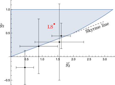
Figure 9: Experimental points for real-world QCD (table 1) with their uncertainties compared to the exclusion plot at Mandelstam order $n=15$. They all lie relatively close to the Skyrme line connecting the origin to the kink. The red dot marks the position of the Lovelace-Shapiro amplitude.

So, where is QCD? Surprisingly, the experimental points in figure 9 gather around the Skyrme line. But they spread all along it, and it would certainly be unwarranted to conclude that QCD sits at the kink. They do suggest, though, that QCD (at least in the chiral and large $N$ limits) lies somewhere in our plot close to the lower-right bound, making this region the most interesting part of the plot.

4.4.4 The Lovelace-Shapiro amplitude

The Lovelace-Shapiro amplitude (22) was an explicit example of a theory satisfying all of our assumptions, so it better be allowed by our bounds. We can compute its position in the space of couplings $(\tilde{g}_{2}^{\prime},\tilde{g}_{2})$ as a consistency check. From (22) we extract

$$\tilde{g}_{2\,{\rm LS}}=-\frac{\gamma+\psi(\frac{1}{2})}{2}\simeq 0.693147\,,\quad\tilde{g}^{\prime}_{2\,{\rm LS}}=2\tilde{g}_{2\,{\rm LS}}\simeq 1.38629\,,$$ (75)

where $\gamma$ is the Euler-Mascheroni constant and $\psi(z)$ the digamma function. This point indeed sits in the interior of the allowed region in figure 9, as it should.

4.5 Comparing with previous work

The program of constraining pion scattering amplitudes from the simple assumptions of unitarity, crossing symmetry and boundedness has a long history dating back to the ’60s Martin1969 . Naturally, not all of our results are new. For example, the positivity of the low-energy coefficients $\ell_{2}\geq 0$ and $\ell_{1}+\ell_{2}\geq 0$ has been known since time immemorial Pham:1985cr ; Adams:2006sv . In our language, these translate into $\tilde{g}_{2}^{\prime}\geq 0$ and $4\tilde{g}_{2}-\tilde{g}_{2}^{\prime}\geq 0$ (i.e. the “Skyrme line”). Similarly, some lower bounds on the combination of couplings $\bar{\ell}_{1}+2\bar{\ell}_{2}$ were derived long ago Ananthanarayan:1994hf ; Pennington:1994kc . Recently, with the improvement of computational power, there has been a resurgence of this program using a variety of methods that have led to a menagerie of new bounds. In this subsection we compare our results with a few recent papers.

In a very nice recent work Alvarez:2021kpq (which builds on Manohar:2008tc ; Mateu:2008gv ), they derived bounds for the chiral Lagrangian using techniques similar to ours. Although the core idea of using dispersion relations to bound the low-energy coefficients is shared by both approaches, there are significant differences that we now outline. On the one hand, they consider massive pions and include loops in chiral perturbation theory (that correspond to $1/N$ corrections), which makes their results much closer to nature, while our target is the Platonic ideal of large $N$ QCD in the chiral limit, of which the real world is but an imperfect shadow.

On the other hand, their method does not exploit all the constraints that the dispersion relations provide. The reason is that they truncate the low-energy amplitude either to $O(p^{4})$ or to $O(p^{6})$ (respectively, NLO or NNLO in chiral perturbation theory). Keeping all orders in (3.1) allowed us to derive an infinity of null constraints that we took into account completely (up to numerical convergence, which seems quite fast). Null constraints Caron-Huot:2020cmc ; Tolley:2020gtv are the key improvement that allowed us to use all the information hidden in the dispersion relations. In addition, since they work at finite $N$, their Regge behavior is worse than (21) and they need at least two subtractions, reducing the number of constraints they have access to.

To see explicitly how the improvements from the full set of null relations come about, consider truncating the low-energy amplitude (3.1) to order $O(p^{4})$ and using only twice-subtracted dispersion relations. Expanding (29) for $k=2$ around the forward limit yields the sum rules

$$g_{2,0}=\Big{\langle}\frac{1}{m^{4}}\Big{\rangle}\,,\qquad g_{2,0}-g_{2,1}=\Big{\langle}\frac{(-1)^{J}}{m^{4}}\Big{\rangle}\,.$$ (77)

Summing them and using positivity of the high-energy average then gives the bound

$$\left(4\tilde{g}_{2}-\tilde{g}_{2}^{\prime}\right)\frac{g_{1,0}}{2M^{2}}=2g_{2,0}-g_{2,1}=\Big{\langle}\frac{1+(-1)^{J}}{m^{4}}\Big{\rangle}\geq 0\,.$$ (78)

Subtracting them yields $g_{2,1}=\Big{\langle}\frac{1-(-1)^{J}}{m^{4}}\Big{\rangle}\geq 0$. In terms of the low-energy couplings (69) these bounds correspond to $\ell_{1}+\ell_{2}\geq 0$ and $\ell_{2}\geq 0$, respectively. This is the result at large $N$. To compare to finite $N$ results, we would have to include low-energy loops from the start, but we can see the qualitative effect of the loops by “running up” the couplings from $m_{\rho}$ to $m_{\pi}$ using (76). This yields the bounds

$$\bar{\ell}_{1}+2\bar{\ell}_{2}\geq 3\log\frac{m_{\rho}^{2}}{m_{\pi}^{2}}\simeq 10.3\,\text{MeV}\,,\qquad\bar{\ell}_{2}\geq\log\frac{m_{\rho}^{2}}{m_{\pi}^{2}}\simeq 3.43\,\text{MeV}\,,$$ (79)

which are comparable to figure 6 of Alvarez:2021kpq . Including terms of order $O(p^{6})$ and using more subtractions brings in the first null constraint, which we can use to place two-sided bounds on the couplings as in figure 7 of Alvarez:2021kpq . But for the complete bounds that reveal the kink we need to keep $M_{\text{low}}(s,u)$ to all orders and use all the dispersion relations with one or more subtractions.

Another approach that has proven successful in the recent years is the numerical S-matrix bootstrap developed in Paulos:2017fhb , which was first applied to massive Guerrieri:2018uew and then to massless Guerrieri:2020bto pions, and has been pursued further in Bose:2020cod ; Bose:2020shm . The optimization method we have used to obtain our positivity bounds solves a dual problem, where one systematically rules out more and more points as more constraints are introduced. This method, in contrast, solves a primal problem, in which points are progressively ruled in. Both methods should be regarded as complementary and they should be pushed until their solutions match, at which point one can be sure that the bounds are optimal. Sadly, our results are not directly comparable to any of these references because we do not tackle exactly the same problem.

The closest one is Guerrieri:2020bto , where they also consider massless pions, but they work at one-loop level in chiral perturbation (i.e. next-to-leading order in $1/N$) and they do not assume a mass gap $M$ before the first resonance. Yet, it is instructive to rewrite our results in their notation. For the low-energy amplitude, they use the one-loop result

$$A(s|t,u)=\frac{s}{f_{\pi}^{2}}+\frac{1}{f_{\pi}^{4}}\left[\alpha s^{2}+\beta(t^{2}+u^{2})-\frac{s^{2}}{32\pi^{2}}\log\frac{-s}{f_{\pi}^{2}}-\frac{t-u}{96\pi^{2}}\left(t\log\frac{-t}{f_{\pi}^{2}}-u\log\frac{-u}{f_{\pi}^{2}}\right)\right]+\cdots$$ (80)

Neglecting loops, we can relate $\alpha$ and $\beta$ to our parameters as

$$g_{1}=\frac{1}{2f_{\pi}^{2}}\,,\quad g_{2,0}=\frac{\alpha+3\beta}{2f_{\pi}^{4}}\,,\quad g_{2,1}=\frac{\beta}{f_{\pi}^{4}}\,,$$ (81)

which gives

$$\alpha=\left(\tilde{g}_{2}-\frac{3}{4}\tilde{g}_{2}^{\prime}\right)\frac{f_{\pi}^{2}}{M^{2}}\,,\qquad\beta=\frac{\tilde{g}_{2}^{\prime}}{4}\frac{f_{\pi}^{2}}{M^{2}}\,.$$ (82)

Figure 10 shows our results in this new parametrization so that they can be (morally) compared with figure 1 of Guerrieri:2020bto .

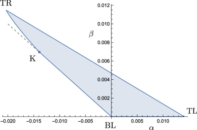
Figure 10: Final exclusion plot from figure 6 in the parametrization (82). This plot is to be compared with figure 1 of Guerrieri:2020bto . We used the values $M=m_{\rho}\simeq 775\,$MeV as our cutoff scale and $f_{\pi}\simeq 92\,$MeV.

Both plots agree on the lower bounds $\beta\geq 0$, $\left(\alpha+2\beta\right)\geq 0$, which are reached asymptotically in their case. These are precisely the bounds that we derived around (78). In Guerrieri:2020bto they give a dispersive argument for these bounds analogous to ours. A clear difference between both figures, though, is that ours also has upper bounds for $\alpha$ and $\beta$. This is due to the assumption of the mass gap $M$ corresponding to the mass of the rho. Notably, our plots do not overlap. The reason for this is that we have neglected loops. As discussed above, the effect of the loops from the tree-level point of view is to make the couplings run, so including them would shift our plot and make them overlap. It would be interesting to include low-energy loops (i.e.  $1/N$ corrections) in our approach from the start and look for better agreement with the results of Guerrieri:2020bto .

Finally, an interesting method for constraining scattering amplitudes was developed in Haldar:2021rri ; Raman:2021pkf using geometric function theory. It was then applied to pions in Zahed:2021fkp . This method yields uncorrelated bounds for each Wilson coefficient, i.e. a set of allowed intervals. Thus, while they are easier to compute, these constraints do not capture the rich geometry of the space of healthy EFTs (e.g. the kink). We could not compare our results with Zahed:2021fkp because it seems essential for them to consider massive pions and also because they do not find bounds for the couplings $\tilde{g}_{2},$ $\tilde{g}_{2}^{\prime}$. This is probably due to the fact that they only use dispersion relations for fully crossing-symmetric combinations of the pion amplitude, which reduces the number of constraints and prevents from reaching the lowest-lying coefficients.

5 Including the rho

We can make another step towards QCD by modifying our low-energy EFT to account for the exchange of the rho meson, the first state that contributes to pion scattering at large $N$ (see the discussion in appendix A). In nature, the $\rho^{a}_{\mu}$ meson is an $SU(2)$ isospin triplet of spin $J=1$ and mass $m_{\rho}$. More generally, we will consider a massive spin-one particle in the adjoint representation of $SU(N_{f})$, which we will continue to call $\rho^{a}_{\mu}$ ($a=1,\ldots,N_{f}^{2}-1$). Such a particle can only interact with two pions via an interaction term of the form

$$\mathcal{L}_{\text{int}}=-g_{\pi\pi\rho}\,f_{abc}\pi^{a}\partial^{\mu}\pi^{b}\rho^{c}_{\mu}\,,$$ (83)

as discussed in appendix B, and in the $N\to\infty$ limit this is all we need since only tree-level diagrams survive. The low energy $\pi\pi\to\pi\pi$ scattering amplitude for an EFT including such an interaction term (together with a kinetic and mass terms for the rho) is computed with the diagrams of figure 11, and it has the form of (2.1) with

$$A_{\text{low}}^{(\rho)}(s|t,u)=g_{\pi\pi\rho}^{2}\left(\frac{m_{\rho}^{2}+2s}{m_{\rho}^{2}-u}+\frac{m_{\rho}^{2}+2s}{m_{\rho}^{2}-t}\right)+\text{analytic}\;.$$ (84)

Figure 11: Feynman diagrams contributing to the $2\to 2$ scattering of pions for an EFT including the rho. At large $N$ only tree-level diagrams survive. There is the explicit exchange of the rho and an infinite series of 4-point vertices coming from integrating out the heavier mesons in the spectrum.

Using (6), this yields the following new low-energy amplitude,

$$M_{\text{low}}^{(\rho)}(s,u)=\frac{1}{2}g_{\pi\pi\rho}^{2}\left(\frac{m_{\rho}^{2}+2u}{m_{\rho}^{2}-s}+\frac{m_{\rho}^{2}+2s}{m_{\rho}^{2}-u}\right)+\sum_{n=0}^{\infty}\sum_{\ell=0}^{[n/2]}\hat{g}_{n,\ell}\left(s^{n-\ell}u^{\ell}+u^{n-\ell}s^{\ell}\right)\,.$$ (85)

This amplitude is crossing-symmetric in $s\leftrightarrow u$ and it has a pole (for fixed $u$) at $s=m_{\rho}^{2}$ with residue $-\frac{1}{2}g_{\pi\pi\rho}^{2}m_{\rho}^{2}\,\mathcal{P}_{1}\left(1+\frac{2u}{m_{\rho}^{2}}\right)$, which is consistent with unitarity as long as $g_{\pi\pi\rho}^{2}\geq 0$. Note that we have written hats on top of the $g_{n,\ell}$ couplings to emphasize that these coefficients are different from those in (3.1). Integrating out the rho would bring back the original coefficients $\hat{g}_{n,\ell}\to g_{n,\ell}$. At the level of the amplitude, integrating out the rho is as simple as Taylor-expanding the poles around $s,u\sim 0$, which we can do safely for energies below the mass of the rho. The precise relation between the couplings is

$$g_{1,0}=\hat{g}_{1,0}+\frac{3}{2}\frac{g_{\pi\pi\rho}^{2}}{m_{\rho}^{2}}\,, g_{n,1}=\hat{g}_{n,1}+\frac{g_{\pi\pi\rho}^{2}}{m_{\rho}^{2n}}\quad n=2,3,\dots\,,$$

$$g_{n,0}=\hat{g}_{n,0}+\frac{1}{2}\frac{g_{\pi\pi\rho}^{2}}{m_{\rho}^{2n}}\quad n=2,3,\dots\,,\quad g_{n,\ell}=\hat{g}_{n,\ell}\phantom{+\frac{g_{\pi\pi\rho}^{2}}{m_{\rho}^{2n}}}\;\,\,\left\{\begin{aligned} n&=4,5,\dots\,\\ \ell&=2,\dots,\left[\tfrac{n}{2}\right]\,.\end{aligned}\right.$$ (86)

In the previous section, we used the original EFT amplitude (3.1) for energies up to the cutoff scale $M$. When considering QCD, this cutoff can be pushed only up to $m_{\rho}$. Beyond this scale, one must use the new amplitude $M_{\text{low}}^{(\rho)}$ including the rho pole. Despite having the explicit rho, this amplitude is still an EFT with all the higher mesons integrated out, so it can in turn only be used up to a new cutoff scale $M^{\prime}>m_{\rho}$ (the mass of the next meson in the spectrum).

The amplitude (85) describes the low-energy physics of any theory with a rho as the first meson exchanged by the pions and, among them, is large $N$ QCD. So we can play the same game as in section 3 with it to carve out the space of such theories allowed by unitarity. This should bring us closer to QCD. Moreover, with this low-energy amplitude we gain access to the more experimentally-available quantities $g_{\pi\pi\rho}^{2}$, $m_{\rho}$. We can try to put bounds on these quantities as well.

5.1 “New” sum rules and null constraints

The naive way of treating this new amplitude is to separate low and high energies by the new cutoff $M^{\prime}$ so that the contour at low energies steps on two poles; zero and $m_{\rho}^{2}$ (see figure 12(a)). In this approach we would simply have to use (85) in the left hand side of the dispersion relations (29) and consider high-energy averages integrating over masses $m\geq M^{\prime}$. Expanding in $u$ would then yield new null constraints and sum rules for the couplings $\hat{g}_{n,\ell}$, $g_{\pi\pi\rho}$ that we could use in a dual problem like the one in section 4.1. However, it is much more efficient and illuminating to keep the rho pole in the high-energy side of the dispersion relations. That is, to use the fully analytic amplitude (3.1) (with $g_{n,\ell}$ couplings) around the origin and consider as high-energy spectrum an isolated rho pole together with a continuum starting above $M^{\prime}$ (see figure 12(b)).

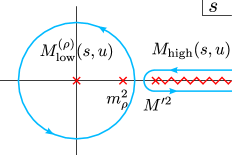
(a) rho at low energies

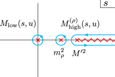
(b) rho at high energies

Figure 12: There are two equivalent ways of dealing with the rho: (a) including it at low energies or (b) keeping it at high energies. We will go with the latter. The analogous contours for the ST sum rules also have poles on the negative $\text{Re}\,s$ axis.

This is achieved by shifting the high-energy spectral density by

$$n_{J}^{(D)}\rho_{J}(s)\longrightarrow\frac{\pi}{2}\,g_{\pi\pi\rho}^{2}\delta(s-m_{\rho}^{2})\,\delta_{J,1}\,m_{\rho}^{D-2}+n^{(D)}_{J}\rho_{J}^{\prime}(s)\,,$$ (87)

where $\rho_{J}^{\prime}(s)$ now has support above the new cutoff $M^{\prime}$. This makes a new term pop out from the heavy averages accounting for the isolated rho,

$$\Big{\langle}F\left(m^{2},J\right)\Big{\rangle}\longrightarrow\frac{1}{2}g_{\pi\pi\rho}^{2}\,F\left(m_{\rho}^{2},J=1\right)+\Big{\langle}F\left(m^{2},J\right)\Big{\rangle}^{\prime}\,,$$ (88)

where the prime indicates that the averaging is done for masses $m\geq M^{\prime}$. With this replacement it is straightforward to derive the new sum rules and null constraints from the original ones. A few examples are

$$g_{1,0}=\frac{1}{2}\frac{g_{\pi\pi\rho}^{2}}{m_{\rho}^{2}}+\Big{\langle}\frac{1}{m^{2}}\Big{\rangle}^{\prime}\,,\quad g_{2,0}=\frac{1}{2}\frac{g_{\pi\pi\rho}^{2}}{m_{\rho}^{4}}+\Big{\langle}\frac{1}{m^{4}}\Big{\rangle}^{\prime}\,,\quad g_{2,1}=\frac{1}{2}\frac{g_{\pi\pi\rho}^{2}}{m_{\rho}^{4}}+\frac{1}{(D-2)}\Big{\langle}\frac{{\mathcal{J}}^{2}}{m^{4}}\Big{\rangle}^{\prime}\,.$$ (89)

These results could be rearranged into sum rules for the new couplings $\hat{g}_{n,\ell}$ using (5), but as we now discuss, they will be more useful as they are.

5.2 New exclusion plot

The easiest way to compare the allowed region for theories including a rho with the original plot (figure 6) is to look for bounds on the same couplings $g_{n,\ell}$ rather than the new couplings $\hat{g}_{n,\ell}$. We will construct the same plot as before but assuming the high-energy spectrum of figure 12(b) for different values of $M^{\prime}$. Thus, we will be asking how does the allowed region for pion EFTs change as we restrict to theories with a rho as their first meson in the spectrum? And, how does that change as we increase the gap after the rho?

Consider the same vectors as in (53) together with

$$\vec{v}_{\rho}\equiv\vec{v}_{\text{HE}}\left(m_{\rho}^{2},J=1\right)\,,$$ (90)

and normalize them by $m_{\rho}$ (i.e. replace $M\to m_{\rho}$). These vectors now satisfy the bootstrap equation

$$\vec{v}_{\mathbb{1}}+\tilde{g}_{2}\,\vec{v}_{2}+\tilde{g}_{2}^{\prime}\,\vec{v}_{2^{\prime}}+\tilde{g}_{\rho}^{2}\vec{v}_{\rho}+\Big{\langle}\vec{v}_{\text{HE}}\left(m^{2},J\right)\Big{\rangle}^{\prime}=0\,,$$ (91)

where the normalized couplings are defined as

$$\tilde{g}_{2}\equiv g_{2,0}\frac{m_{\rho}^{2}}{g_{1,0}}\,,\qquad\tilde{g}_{2}^{\prime}\equiv 2g_{2,1}\frac{m_{\rho}^{2}}{g_{1,0}}\,,\qquad\tilde{g}_{\rho}^{2}\equiv\frac{1}{2}\frac{g_{\pi\pi\rho}^{2}}{g_{1,0}\,m_{\rho}^{2}}\,.$$ (92)

Compared to (54), in this bootstrap equation the heavy states consist of the isolated $\vec{v}_{\rho}$ and the continuum $\vec{v}_{\text{HE}}$. So we can construct the new exclusion plot by following the same program from section 4.2 with the positivity condition (step 2) updated to

$$\vec{\alpha}\cdot\vec{v}_{\rho}\geq 0\,,\qquad\vec{\alpha}\cdot\vec{v}_{\text{HE}}\left(m^{2},J\right)\geq 0\quad\forall J,\,m\geq M^{\prime}\,,$$ (93)

for fixed values of $M^{\prime}$ and $m_{\rho}$.

Out of the two mass scales of this problem, only the ratio $M^{\prime}/m_{\rho}$ is meaningful, but the bounds change by an overall rescaling depending on which mass we use to normalize the couplings in (92). We have chosen to normalize everything on $m_{\rho}$ so that raising $M^{\prime}$ corresponds to enlarging the gap after a fixed rho rather than moving down the rho under a fixed cutoff. Figure 13 shows how the exclusion plot changes as a function of this gap.

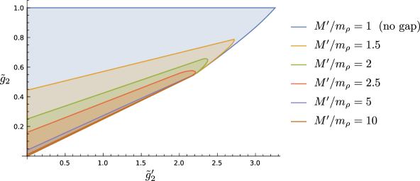
Figure 13: Exclusion plot in the space of couplings $(\tilde{g}_{2}^{\prime},\tilde{g}_{2})$ when the high-energy spectrum contains an isolated rho below a cutoff $M^{\prime}$, for different values of $M^{\prime}/m_{\rho}$. All the plots were computed at Mandelstam order $n=7$. At $M^{\prime}/m_{\rho}=1$ the allowed region matches figure 6, and when $M^{\prime}/m_{\rho}\to\infty$ it shrinks towards the Skyrme line connecting the origin to the kink.

For $M^{\prime}/m_{\rho}=1$, there is no gap after the rho and hence the plot reduces to the original one (figure 6). This is the most permissive assumption we can make, since it allows for virtually any UV completion, and so it yields the biggest allowed region. As we raise $M^{\prime}$, we restrict ourselves to theories with a larger and larger gap and the region shrinks. Already for relatively small gaps, the allowed region shrinks significantly towards the lower-right part of the plot, indicating that this is where the theories with a rho as their first internal state congregate. Astonishingly, as we push $M^{\prime}$ very high, the allowed region shrinks onto the Skyrme line connecting the origin to the kink, which seems to survive all the way to $M^{\prime}/m_{\rho}\to\infty$.

This is an interesting result. It implies that one can construct “healthy theories” (i.e. crossing-symmetric, unitary and spin-one Regge bounded) out of a single rho and infinitely heavy mesons. Moreover, these theories must lie on the Skyrme line. So, at the kink there must live at least a funny UV completion of a spin-one particle, but this is not necessarily the whole story. Our bounds show the allowed region for theories that meet our assumptions; they have nothing to say about theories that do not satisfy them. So it could well be that the kink is also populated by other theories with a much different spectrum.

For QCD, the cutoff $M^{\prime}$ can only be pushed as high as the next meson in the spectrum, and one might naively conclude that we will rule out QCD when $M^{\prime}/m_{\rho}$ is taken high enough. But we cannot make such a statement. Again, our bounds ensure that any theory compatible with the assumed spectrum will live inside the allowed region, but they do not force all the theories that fall within the bounds to have the assumed spectrum. For example, a healthy theory with a fixed gap of –say– $M^{\prime}/m_{\rho}=1.5$ will lie inside the light orange area of figure 13, but it can either fall inside or outside the green region. Therefore, while we have something of a candidate for a theory living at the kink, the possibility that large $N$ QCD sits on top of it remains open.

5.3 The rho coupling

Let us continue our quest for QCD by studying what values of the rho coupling $g_{\pi\pi\rho}$ are allowed by unitarity. To do so, one might be tempted to rearrange the new null constraints resulting from (88) into a function $g_{\pi\pi\rho}^{2}(m^{2},J)$ whose high-energy average gives $g_{\pi\pi\rho}^{2}$ and then use it in a dual problem like in section 4.1. However, with our reformulation of the dual problem in terms of bootstrap equations, we do not have to work so hard to bound $g_{\pi\pi\rho}^{2}$. Indeed, the vectors

$$\vec{v}_{\mathbb{1}}=\begin{pmatrix}1\\ 0\\ \vdots\\ 0\end{pmatrix}\,,\qquad\vec{v}_{\text{HE}}\left(m^{2},J\right)=\begin{pmatrix}-g_{1,0}\left(m^{2},J\right)m_{\rho}^{2}\\ \mathcal{Y}_{2,1}\left(m^{2},J\right)m_{\rho}^{4}\\ \mathcal{X}_{3,1}\left(m^{2},J\right)m_{\rho}^{6}\\ \vdots\end{pmatrix}\,,\quad\vec{v}_{\rho}\equiv\vec{v}_{\text{HE}}\left(m_{\rho}^{2},J=1\right)\,,$$ (94)

defined with the same sum rules and null constraints from section 3, satisfy the bootstrap equation

$$\vec{v}_{\mathbb{1}}+\tilde{g}_{\rho}^{2}\vec{v}_{\rho}+\Big{\langle}\vec{v}_{\text{HE}}\left(m^{2},J\right)\Big{\rangle}^{\prime}=0\,.$$ (95)

This has the form of (46) with $\vec{v}_{\rho}$ the operator whose “OPE coefficient” we want to bound. We can thus obtain bounds for $\tilde{g}_{\rho}^{2}$ directly by applying the same program from section 4.1 to these vectors. The key point is that by normalizing the functional $\vec{\alpha}$ on $\vec{v}_{\rho}$ we avoid having to derive a sum rule for $g_{\pi\pi\rho}^{2}$.

Either way, we can systematically apply this program using SDPB sdpb to place bounds on $\tilde{g}_{\rho}^{2}$ for different fixed values of the cutoff $M^{\prime}$. This yields the upper bounds shown in figure 14. The highest allowed value for $\tilde{g}_{\rho}^{2}$ happens for $M^{\prime}=m_{\rho}$ (when there is no gap), where we have

$$\tilde{g}_{\rho}^{2}\leq 0.776674...\,.$$ (96)

The lower bounds one gets from this program are always negative, but we know that $g_{\pi\pi\rho}^{2}\geq 0$ for the rho pole to be unitary, so they are meaningless.

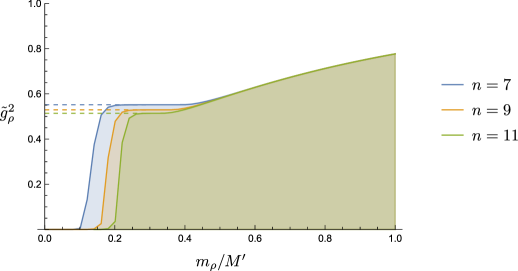
Figure 14: Upper bounds for the normalized coupling of the rho, $\tilde{g}_{\rho}^{2}\equiv\frac{1}{2}\frac{g_{\pi\pi\rho}^{2}}{g_{1,0}\,m_{\rho}^{2}}$, as a function of the gap between the rho and the higher mesons in the spectrum (starting above the cutoff scale $M^{\prime}$). The different plots were made using all the null constraints up to Mandelstam order $n=7,9,11$. The sharp edges to the left of the plots are a numerical artifact (see figure 15); the dashed lines delineate the true bounds.

A surprising feature of figure 14 is the sudden jumps at the left part of the plots. This is purely a numerical artifact from the truncation in spins that we discussed in section 4.1. As shown in figure 15, increasing the spin cutoff $J_{\text{max}}$ pushes the bound further to the left, so the true bounds have a plateau that extends all the way to $m_{\rho}/M^{\prime}=0$. Thus, we find once again that there must exist some healthy theory with just a rho and all the higher mesons pushed to infinity, like we saw in figure 13.

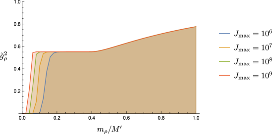
Figure 15: Convergence in spins for the plot in figure 14 at Mandelstam order $n=7$. The right part of the plot converges quickly in spins. In contrast, the steep descent at the left moves further to the left as we increase $J_{\text{max}}$, indicating that the plateau extends all the way to the $y$-axis when convergence is achieved.

Returning to figure 14, we see that the bounds separate into two regions of distinct behavior; a smooth curve to the right of $m_{\rho}/M^{\prime}\sim 0.4$ and a plateau to the left. While the curve has already converged in $n$, the plateau has not. Surprisingly, we have found that for each value of $n$ the value of $\tilde{g}_{\rho}^{2}$ at the plateau matches exactly with the value of $\tilde{g}_{2}$ at the kink for the corresponding plot in figure 6! Which raises the quesion: what is the origin of this connection? and are any of these features related to large $N$ QCD? We will shed some light into this mysterious relation in section 6, but for the moment this observation suggests that the convergence of the plateau is also given by figure 7. The plateau would then converge towards $\tilde{g}_{\rho}^{2}\sim 0.42$.

5.4 Hidden local symmetry and vector meson dominance

The standard chiral Lagrangian (4.4.1) is an EFT only for pions. In general, to include the rho we would have to include all the interaction terms allowed by the symmetries of the problem together with the corresponding unknown coefficients. There is a notorious model, whose fundamental significance is still very much unclear, where the rho meson is treated as the dynamical gauge boson of a “hidden local symmetry” (HLS) of the chiral Lagrangian Bando:1984ej ; Bando:1987br (see Komargodski:2010mc for a nice discussion). This ansatz reduces the number of unfixed coefficients, giving relations between different physical quantities that agree surprisingly well with phenomenological observations. Let us see what our bounds can say about this model.

In a nutshell, if the matrix $U(x)\in SU(N_{f})$ of the chiral Lagrangian is rewritten as a product of two special unitary matrices $U(x)=\xi_{L}(x)\xi_{R}(x)^{\dagger}$, apart from the global chiral symmetry $SU(N_{f})_{L}\otimes SU(N_{f})_{R}$ acting as

$$\xi_{L}(x)\to g_{L}\xi_{L}(x)\,,\qquad\xi_{R}(x)\to g_{R}\xi_{R}(x)\,,$$ (97)

the system enjoys an additional $\left[SU(N_{f})\right]_{\text{local}}$ symmetry

$$\xi_{L}(x)\to\xi_{L}(x)h(x)\,,\qquad\xi_{R}(x)\to\xi_{R}(x)h(x)\,.$$ (98)

Of course, this “hidden symmetry” just indicates that the new parametrization is redundant, but now we can incorporate the corresponding dynamical gauge field $\rho_{\mu}^{a}$ and interpret it as the rho meson. The idea is that its mass should be generated (somehow) via the Higgs mechanism.

The Lagrangian is then obtained by writing down all the $L\leftrightarrow R$ symmetric terms compatible with both the global and local symmetries. At two-derivative order, it reads

$$\mathcal{L}_{\text{HLS}}=-\frac{1}{2g^{2}}\text{Tr}\left(F_{\mu\nu}F^{\mu\nu}\right)-\frac{f_{\pi}^{2}}{4}\text{Tr}\left(\left(\rho_{\mu}^{L}-\rho_{\mu}^{R}\right)^{2}\right)-a\frac{f_{\pi}^{2}}{4}\text{Tr}\left(\left(\rho_{\mu}^{L}+\rho_{\mu}^{R}\right)^{2}\right)+\cdots\,,$$ (99)

where

$$\rho_{\mu}^{L}=\rho_{\mu}^{a}T_{a}-i\xi_{L}^{\dagger}\partial_{\mu}\xi_{L}\,,\qquad\rho_{\mu}^{R}=\rho_{\mu}^{a}T_{a}-i\xi_{R}^{\dagger}\partial_{\mu}\xi_{R}\,.$$ (100)

There are two free parameters; the “gauge coupling” $g$ and an arbitrary coefficient $a$. The normalization of the second term is fixed in terms of $f_{\pi}$ by requiring that this Lagrangian reproduces the leading term of the chiral Lagrangian (4.4.1) upon integrating out the rho.

By picking the unitary gauge $\xi_{L}(x)=\xi_{R}^{\dagger}(x)\equiv\exp\left[\frac{i}{f_{\pi}}T_{a}\pi^{a}(x)\right]$ and expanding in pion fields it is easy to see that $\mathcal{L}_{\text{HLS}}$ includes a single $\pi\pi\rho$-interaction term, which has the form of (83) with coupling

$$g_{\pi\pi\rho}=\frac{1}{2}ga\,.$$ (101)

There is also a mass term for the gauge boson $\rho_{\mu}^{a}$, due to the higgsing of $\left[SU(N_{f})\right]_{\text{local}}$, with mass

$$m_{\rho}^{2}=ag^{2}f_{\pi}^{2}\,.$$ (102)

Apart from these two quantities, the assumption that the rho meson arises as the gauge boson for a HLS relates other couplings to the basic paramaters $g$ and $a$. Namely, the three- and four-rho couplings are proportional to $g$ and $g^{2}$ respectively, while the $\rho\rho\pi\pi$ coupling is $\sim ag^{2}$. However, in the $2\to 2$ scattering of pions at large $N$ only $g_{\pi\pi\rho}$ and $m_{\rho}$ show up, cf. (85). Since there is a total of two independent parameters, $m_{\rho}$ and $g_{\pi\pi\rho}$ are independent and we can use (99) to describe any amplitude allowed by our bounds. So our results cannot test HLS per se. To do so, one would need to consider new processes, such as $\pi\pi\to\rho\rho$ or $\rho\rho\to\rho\rho$ to gain access to the remaining couplings and check if the relations imposed by HLS are allowed by unitarity. Considering the full system of mixed $2\to 2$ amplitudes involving pions and rhos is an important direction for future work.

There is nevertheless one thing we can assess: the parameter tuning that corresponds to “rho dominance”. This is the choice $a=2$ in the HLS Lagrangian, as motivated by several phenomenological observations Bando:1984ej . First, for this value of $a$, the HLS Lagrangian predicts $g_{\pi\pi\rho}=g$, which explains the universality of the rho coupling Sakurai . Second, the mass and the rho coupling satisfy the celebrated KSRF relation Kawarabayashi:1966kd ; Riazuddin:1966sw ,

$$m_{\rho}^{2}=2g_{\pi\pi\rho}^{2}f_{\pi}^{2}\,,$$ (103)

observed empirically. And third, (after extending (99) to account for interactions with photons) one sees that for $a=2$ the electromagnetic form factor of the pion (in this ultrasimplified model, of course) only receives contributions from the rho; this is known as rho dominance (or vector meson dominance) Sakurai . With this choice, the normalized coupling of the rho takes the value

$$\tilde{g}_{\rho}^{2}\equiv\frac{1}{2}\frac{g_{\pi\pi\rho}^{2}}{g_{1,0}m_{\rho}^{2}}=\frac{a}{4}=0.5\,,$$ (104)

where we have used $g_{1,0}=\frac{1}{2f_{\pi}^{2}}$, as derived in (68) for the chiral Lagrangian. This result is plotted against our bounds in figure 16.

In this figure we have included, apart from the bound at order $n=11$, the extrapolation to $n\to\infty$ obtained from fitting the data in figure 14 to get a rough idea of the final shape of the bound once convergence in $n$ is achieved. From the relation between the plateau and the position of the kink in figure 6 noted above, though, we actually expect the plateau to move further down to a value around $\tilde{g}_{\rho}^{2}\sim 0.42$ when more values of $n$ are used. Since the plateau inevitably converges to a value below $0.5$, the KSRF line intersects with the bound and thus (103) is only allowed for values of $m_{\rho}/M^{\prime}$ greater than $\sim 0.38$.

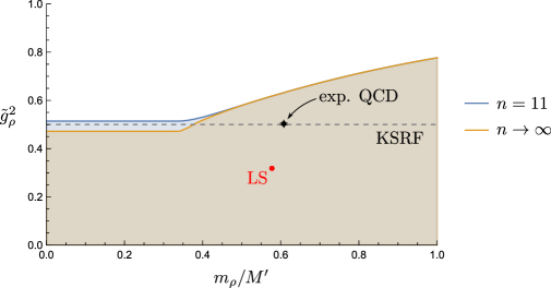
Figure 16: Location of different amplitudes inside the bounds for $\tilde{g}_{\rho}^{2}$. The blue curve is the bound computed at Mandelstam order $n=11$ while the orange one is the projected convergence of the bound obtained from fitting the lower values of $n$. The gray dashed line corresponds to the KSRF relation Kawarabayashi:1966kd ; Riazuddin:1966sw , while the red and black dots mark, respectively, the location of the Lovelace-Shapiro amplitude and real-world QCD. For QCD, the experimental error bars are comparable to the size of the dot.

We can further study the HLS model by integrating out the rho from (99) so as to recover the chiral Lagrangian with a particular combination of low energy couplings. As discussed e.g. in Zahed:1986qz , this yields precisely the Skyrme model (71). To integrate out a “heavy” rho we must plug its equation of motion,

$$\rho_{\mu}^{a}T_{a}=\frac{i}{2}\left(\xi_{L}^{\dagger}\partial_{\mu}\xi_{L}+\xi_{R}^{\dagger}\partial_{\mu}\xi_{R}\right)\,,$$ (105)

back into (99). With this replacement, the last term in (99) vanishes exactly and the second term (which is actually independent of $\rho_{\mu}^{a}$) matches the leading term of the chiral Lagrangian. Meanwhile, the kinetic term for the rho (at leading order in derivatives) reproduces the Skyrme term

$$-\frac{1}{2g^{2}}\text{Tr}\left(F_{\mu\nu}F^{\mu\nu}\right)=\frac{1}{32g^{2}}\text{Tr}\left(\left[U^{\dagger}\partial_{\mu}U,U^{\dagger}\partial_{\nu}U\right]\left[U^{\dagger}\partial^{\mu}U,U^{\dagger}\partial^{\nu}U\right]\right)\,.$$ (106)

So, by integrating out the rho and truncating at four-derivative order, we indeed recover the Skyrme model (71) with the free parameter identified with the gauge coupling; $e=g$.

Thus, in the space of two-derivative couplings (figure 6), this theory sits on the Skyrme line at a value

$$\tilde{g}_{2}=\frac{1}{4g^{2}}\frac{M^{2}}{f_{\pi}^{2}}=\frac{a}{4}\,.$$ (107)

For the special choice of $a=2$, we get $\tilde{g}_{2}=0.5$ and so the HLS model “at the point of rho dominance” sits close to the kink of figure 6. However, according to our numerics (see figure 7), $\tilde{g}_{2}=0.5$ is not quite the kink; which we expect to converge to a value below 0.5 (to approximately $0.42$ according to our $n\to\infty$ extrapolation). In fact, the bound at $n=15$ (59) already rules out this point. This means that (99) with the choice $a=2$ is not compatible with unitarity as is; $\mathcal{L}_{\text{HLS}}$ is too simple of a model. Of course, higher-derivative corrections to it would change the values of $\tilde{g}_{2},\tilde{g}_{2}^{\prime}$ and may restore unitarity.

5.5 Comparing with experiment

We end this section by locating real-world QCD in the plot of the rho coupling bound. There are several ways of determining $g_{\pi\pi\rho}$ Sakurai:1966zza . The most direct one is to use experimental results for the decay width of $\rho\to\pi\pi$ and compare to

$$\Gamma_{\rho\to\pi\pi}=\frac{g_{\pi\pi\rho}^{2}}{48\pi}m_{\rho}\left(1-\frac{4m_{\pi}^{2}}{m_{\rho}^{2}}\right)^{\frac{3}{2}}\,.$$ (108)

From the current measured values $\Gamma_{\rho\to\pi\pi}=149.1\pm 0.8\,$MeV, $m_{\pi}\simeq 139.57\,$MeV PDG , we get $g_{\pi\pi\rho}^{2}=35.7\pm 0.2$, which in turn yields

$$\tilde{g}_{\rho}^{2}=g_{\pi\pi\rho}^{2}\frac{f_{\pi}^{2}}{m_{\rho}^{2}}=0.503\pm 0.003\,.$$ (109)

This agrees very well with the KSRF relation (104).

As for the value of the cutoff $M^{\prime}$, it can only be pushed up to the next meson in the spectrum after the rho. As discussed in appendix A, for large $N$ QCD this is the $f_{2}(1270)$, which has mass $M^{\prime}=1275.5\pm 0.8\,$MeV PDG .

With these coordinates in hand, we can place real-world QCD in the allowed region for the rho coupling, see figure 16. For reference, we have also added the point that corresponds to the Lovelace-Shapiro amplitude, which has $m_{\rho}/M^{\prime}=1/\sqrt{3}$, $\tilde{g}_{\rho}^{2}=1/\pi$. Comfortingly, both points are allowed by our bounds, but QCD appears to be rather far from the boundary and so we cannot make a precise connection with any feature of the plot. Note, however, that although the experimental error bars for real-world QCD are very small, one should always keep in mind that we are comparing it to the large $N$ theory in the chiral limit, so there is room for larger discrepancies.

6 Understanding the geometry of the bounds

It is an outstanding question to understand the geometry of positivity bounds from a more analytic point of view. While we have seen some intriguing connections to old hadron phenomenology that might indicate that QCD sits in the vicinity of the kink, we have also found evidence that a simpler theory lives at that point. In Caron-Huot:2020cmc it was shown that some positivity bounds for EFTs can be saturated by very simple amplitudes satisfying crossing, unitarity and Regge boundedness. So it could be that the kink is just a spurious solution that prevents us from reaching more interesting parts inside our plot. In this section we organize the evidence for this hypothesis and engineer an example that rules in a significant part of the exclusion plot. We would like to stress, though, that even if such a simple amplitude saturating the bounds is eventually found, it could still be that different theories (like large $N$ QCD) sit on top of it. The way to go would then be to make further assumptions that are true for large $N$ QCD but not for the spurious solution and see whether the kink survives or not.

6.1 Analytically ruling in

As discussed in section 4.5, there is a complementary method to the dual problem that we have used; the primal problem. The difference being that the former progressively rules out more points of the space of EFTs while the latter rules them in. In a primal problem, one looks for examples of EFTs that satisfy our assumptions in order to say that a given point is allowed. When the bounds of both methods agree, we know that they are optimal. This approach has been applied numerically to pion scattering in Guerrieri:2018uew ; Guerrieri:2020bto ; Bose:2020cod ; Bose:2020shm , but in Caron-Huot:2020cmc they introduced an alternative —and very insightful— way of answering this question, which consists in ruling in amplitudes analytically. The basic idea is that positivity bounds might be saturated by simple functions $M(s,u)$ satisfying crossing symmetry, unitarity and the assumed Regge behavior. If we manage to find them, not only do we learn that the bounds are optimal, but we also gain a conceptual understanding of the geometry of the bounds.

Following Caron-Huot:2020cmc closely, we tackle first the top bound of figure 6; $\tilde{g}_{2}\leq 1$. From the sum rules

$$g_{1,0}=\Big{\langle}\frac{1}{m^{2}}\Big{\rangle}\,,\qquad g_{2,0}=\Big{\langle}\frac{1}{m^{4}}\Big{\rangle}\,,$$ (110)

it is clear that $\tilde{g}_{2}=\frac{g_{2,0}M^{2}}{g_{1,0}}$ will only reach $1$ on amplitudes that only have states at $m=M$. Any pole at a higher mass would lower $\tilde{g}_{2}$. Apart from the constant amplitude, there are two independent rational amplitudes that are unitary, $s\leftrightarrow u$ symmetric, spin-one Regge bounded and have all states at $s=m^{2}$:

$$M_{\text{spin-0}} \;=\;\frac{m^{2}}{m^{2}-s}+\frac{m^{2}}{m^{2}-u}\,,$$ (111a)

$$M_{su-\text{pole}} \;=\;\frac{m^{4}}{\left(m^{2}-s\right)\left(m^{2}-u\right)}-\alpha_{J=0}^{(D)}M_{\text{spin-0}}\,.$$ (111b)

The former corresponds to the exchange of a single particle of mass $m$ and spin $J=0$, while the spectrum of the latter consists of an infinite tower of spins $J\geq 1$ at mass $m$. In (111b), $\alpha^{(D)}_{J=0}$ is chosen such that it cancels completely the spin-zero contribution.

The contribution from each spin to a given pole is obtained by expanding the residue (at fixed $u$) in Gegenbauer polynomials,

$$M(s,u)\sim\frac{m^{2}\sum_{J=0}^{\infty}\gamma_{J}^{(D)}\mathcal{P}_{J}\left(1+\frac{2u}{s}\right)}{m^{2}-s}\,,$$ (112)

and it can be extracted by using the orthogonality relations of $\mathcal{P}_{J}(x)$, Correia:2020xtr . Specifically, we have

$$m^{2}\gamma_{J}^{(D)}=-\frac{1}{2}\mathcal{N}_{D}\,n_{J}^{(D)}\int_{-1}^{1}dx\,(1-x^{2})^{\frac{D-4}{2}}\mathcal{P}_{J}(x)\,\text{Res}_{s=m^{2}}\Big{[}M\big{(}s,u(x)\big{)}\Big{]}\,,$$ (113)

where $x=1+\frac{2u(x)}{s}$ and $\mathcal{N}_{D}=\frac{(16\pi)^{\frac{2-D}{2}}}{\Gamma\left(\frac{D-2}{2}\right)}$. Applying this for $J=0$ to the first term of (111b) shows that we must choose

$$\alpha_{J=0}^{(D)}=\frac{2}{3}\,{}_{2}F_{1}\left(\frac{1}{2},1,\frac{D-1}{2},\frac{1}{9}\right)\,\qquad(\text{for }D\geq 3)\,,$$ (114)

$$\alpha_{J=0}^{(3)}=\frac{1}{\sqrt{2}}\,,\quad\alpha_{J=0}^{(4)}=\log 2\,,\quad\alpha_{J=0}^{(5)}=12-8\sqrt{2}\,,\,\dots\,,$$

for the subtraction to cancel the contribution from spin 0. The reason for this subtraction is to saturate the unitarity condition; anything greater than (114) would break unitarity for the spin-less pole. Similarly to Caron-Huot:2020cmc , positivity for the spins $J\geq 1$ can be verified with the Froissart-Gribov formula (reviewed e.g. in section 2.4 of Correia:2020xtr ) by noting that (113) becomes proportional to $Q_{J}^{(D)}(3)$, which is a positive function for $D\geq 3$.

By expanding the amplitudes (111) at low energies and comparing to (3.1) we find their coordinates in the space of couplings,

$$M_{\text{spin-0}}: \qquad\tilde{g}_{2}=\frac{M^{2}}{m^{2}}\,,\qquad \tilde{g}^{\prime}_{2}=0\,,\qquad \tilde{g}_{3}=\frac{M^{4}}{m^{4}}\,,$$ (115a)

$$M_{su-\text{pole}}: \qquad\tilde{g}_{2}=\frac{M^{2}}{m^{2}}\,,\qquad \tilde{g}^{\prime}_{2}=\left(\frac{1}{1-\alpha^{(D)}_{J=0}}\right)\frac{M^{2}}{m^{2}}\,,\qquad \tilde{g}_{3}=\frac{M^{4}}{m^{4}}\,.$$ (115b)

These amplitudes are crossing symmetric, unitary and have the correct Regge behavior for any mass $m$, but we can only accept them as long as their poles are above the cutoff $M$. Thus, each of them describes a straight line on the plane $(\tilde{g}_{2}^{\prime},\tilde{g}_{2})$ stretching from the origin, to $\tilde{g}_{2}=1$. Since positive linear combinations of unitary amplitudes remain unitary, these two amplitudes rule in the whole convex hull of their corresponding lines, shown in red in figure 17. The ruled-in region covers an impressively large part of the exclusion plot. In particular, it saturates the left and top bounds and it rules in the three corners of our plot; $\text{BL}=(0,0)$, $\text{TL}=(0,1)$ and $\text{TR}=(\tfrac{1}{1-\log 2},1)\simeq(3.25889135327...,1)$, in perfect agreement with (52). There remains, however, a sliver of the exclusion plot to be ruled in, much like in Caron-Huot:2020cmc .

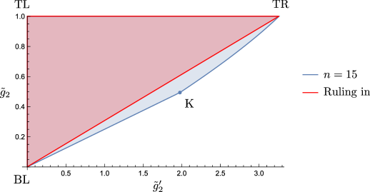
Figure 17: Part of the plane $(\tilde{g}_{2}^{\prime},\tilde{g}_{2})$ ruled in by the amplitudes (111) compared to the numerical ruling out at Mandelstam order $n=15$. The three corners (BL, TL and TR) are ruled in, but there remains a sliver containing the kink (K).

This agreement is not restricted to the plane $(\tilde{g}_{2}^{\prime},\tilde{g}_{2})$. Moving up in dimensions to the space $(\tilde{g}_{2}^{\prime},\tilde{g}_{2},\tilde{g}_{3})$, we find that the lines of the two amplitudes in (111) become parabolas connecting the origin BL to the corners TL and TR. They fall exactly on the blue sheet of figure 8, and the orange sheet is given by their convex hull. Again, there remains a sliver (containing the kink (K)) to be ruled in.

Despite being healthy amplitudes by our criteria, this does not mean that (111) can be realized in physical large $N$ gauge theories. Rather, they should be regarded as spurious solutions that saturate the bounds and keep us from exploring more interesting regions. One could get rid of them by incorporating further assumptions.

Nevertheless, from this exercise we begin to understand how the healthy amplitudes are arranged in the space of couplings according to their spectra: amplitudes with all their poles at infinity lie at the origin and we find lower and lower masses as we move away from it, until we reach the top bound $\tilde{g}_{2}=1$, where all the masses in our amplitudes hit the cutoff $M$. In addition, from the sum rule

$$g_{2,1}=\frac{1}{(D-2)}\Big{\langle}\frac{{\mathcal{J}}^{2}}{m^{4}}\Big{\rangle}\,,\qquad\Big{(}{\mathcal{J}}^{2}\equiv J(J+D-3)\Big{)}$$ (116)

it is clear that the axis $\tilde{g}_{2}^{\prime}=0$ is inhabited by amplitudes that only involve scalars. Higher spins move them away from the axis.

The question is what happens in the remaining sliver, and what amplitude(s) lives at the kink. We now address this question using the extra information that figures 13 and 14 provide. We will discuss the two regions of the right bound separately; first the part below the kink (from BL to K) and then the part above it (from K to TR). In what follows we are going to refer back to figures 13 and 14 multiple times, so this would be a good point to familiarize oneself with them.

6.2 Bound below the kink

Figure 13 was made by assuming a spectrum with a (fixed) isolated rho at the original cutoff $M\equiv m_{\rho}$ and a continuum after a new (moving) cutoff $M^{\prime}$. As $M^{\prime}\to\infty$, the allowed region shrinks all the way to the lower-right bound connecting the origin to the kink; the Skyrme line,

$$\tilde{g}_{2}^{\prime}=4\tilde{g}_{2}\,.$$ (117)

As noted at the end of section 5.2, this implies that on this line there must live (at least) a theory with just a rho in the spectrum and all the higher mesons (if any) pushed to infinity.

The amplitude for the exchange of a single spin-one particle reads

$$M_{\text{spin-1}}\;=\;\frac{m_{\rho}^{2}+2u}{m_{\rho}^{2}-s}+\frac{m_{\rho}^{2}+2s}{m_{\rho}^{2}-u}\,,$$ (118)

since the spin-one Gegenbauer is $\mathcal{P}_{1}\left(1+\frac{2u}{m_{\rho}^{2}}\right)=1+\frac{2u}{m_{\rho}^{2}}$. This amplitude is $s\leftrightarrow u$ symmetric and unitary, but it does not satisfy spin-one Regge behavior due to the factor of $s$ in the numerator of the $u$-channel term. It grows too fast with energy. Thus, this amplitude cannot be ruled in as is. Luckily, there is a straightforward fix for this; we just have to add crossing-symmetric poles at a much higher scale $m_{\infty}$,

$$M_{\text{spin-1}}^{\text{(UV)}}\;=\;\frac{m_{\rho}^{2}+2u}{m_{\rho}^{2}-s}\left(\frac{m_{\infty}^{2}}{m_{\infty}^{2}-u}\right)+\frac{m_{\rho}^{2}+2s}{m_{\rho}^{2}-u}\left(\frac{m_{\infty}^{2}}{m_{\infty}^{2}-s}\right)\,.$$ (119)

Now, the extra power of $s$ in the denominator damps the amplitude at high energies, curing the Regge behavior. At low energies, if $m_{\infty}$ is taken large enough (formally $m_{\infty}\to\infty$), this amplitude reduces to (118). But the $m_{\infty}$ pole cannot be removed altogether since we must step on it at some point to save the Regge behavior.

Of course, we can only accept the amplitude $M_{\text{spin-1}}^{\text{(UV)}}$ if it is unitary. To check this we must expand the residue of each pole in Gegenbauers as in (112) and verify that all the coefficients are positive. At $m_{\rho}$, all the $\gamma_{J}^{(D)}$ are positive and they all tend to zero as $m_{\infty}\to\infty$ except for $\gamma_{1}^{(D)}\to 1$, as expected. At the other pole, $m_{\infty}$, all the coefficients are again positive. We conclude that (119) is a healthy amplitude and we should embrace it. In a sense, the $m_{\infty}$ pole plays the role of a Higgs boson in UV-compleing the spin-one amplitude, but in this case we have an infinite tower of spins. Once again, though, being a “healthy” amplitude by our standards does not make it a physical theory.

The low energy couplings for this UV-completed spin-one amplitude (in the limit $m_{\infty}\to~{}\infty$) are

$$M_{\text{spin-1}}^{\text{(UV)}}:\qquad\tilde{g}_{2}=\frac{1}{3}\frac{M^{2}}{m_{\rho}^{2}}\,,\qquad\tilde{g}^{\prime}_{2}=\frac{4}{3}\frac{M^{2}}{m_{\rho}^{2}}\,,\qquad\tilde{g}_{3}=\frac{1}{3}\frac{M^{4}}{m_{\rho}^{4}}\,,$$ (120)

which satisfy (117). So this amplitude rules in (part of) the Skyrme line! However, since (119) is only allowed for masses $m_{\rho}\geq M$, it only rules in the Skyrme line up to $(\frac{4}{3},\frac{1}{3})$, which is significantly below the kink (even when taking into account the slow convergence from figure 7). Still, it is remarkable that this bound is saturated by such a simple amplitude. What is actually not that surprising is that (119) matches the Skyrme model, since we saw in section 5.4 that the Skyrme model can be obtained from integrating out a single rho meson.

As for an amplitude that reaches the actual kink, it could be a simple modification of (119). Like in the case of (111b), where one has to subtract the spin-zero amplitude to saturate unitarity, one can imagine that subtracting something from (119) will do the job. From the low energy point of view, we would need the subtraction to lower the value of $g_{1,0}$ but leave all the other $g_{n,\ell}$ unchanged. Indeed, if $g_{1,0}$ decreased by

$$g_{1,0}=\frac{3}{m_{\rho}^{2}}\quad\longrightarrow\quad\frac{3-A}{m_{\rho}^{2}}\,,$$ (121)

we would get the normalized couplings

$$M_{\text{spin-1}}^{\text{(UV)}}-M_{\text{(?)}}:\quad\tilde{g}_{2}=\frac{1}{3-A}\frac{M^{2}}{m_{\rho}^{2}}\,,\quad\tilde{g}^{\prime}_{2}=\frac{4}{3-A}\frac{M^{2}}{m_{\rho}^{2}}\,,\quad\tilde{g}_{3}=\frac{1}{3-A}\frac{M^{4}}{m_{\rho}^{4}}\,.$$ (122)

Such an amplitude would still sit on the Skyrme line (117), but it would run further up the line to $(\frac{4}{3-A},\frac{1}{3-A})$, which would match the kink for $A\simeq 0.9757$. The exclusion plot in the plane $(\tilde{g}_{2},\tilde{g}_{3})$, shown in figure 18, provides further evidence that (122) are the correct low-energy coefficients, since the bound in that plot is fitted very well by the parabola $\tilde{g}_{3}=(3-A)\tilde{g}_{2}^{2}$.

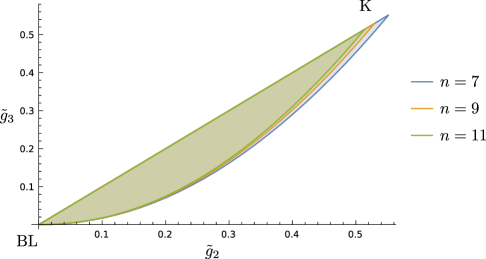
Figure 18: Exclusion plot in the space $(\tilde{g}_{3},\tilde{g}_{2})$ along the Skyrme line $\tilde{g}_{2}^{\prime}=4\tilde{g}_{2}$ extending from the origin (BL) to the kink (K) of figure 6, for Mandelstam orders $n=7,9,11$. The lower bounds are fitted well by the parabolas $\tilde{g}_{3}=\frac{1}{\tilde{g}_{2}^{\text{(K)}}(n)}\,\tilde{g}_{2}^{2}$ with the values of $\tilde{g}_{2}^{\text{(K)}}(n)$ given in figure 7.

But what can we subtract from $M_{\text{spin-1}}^{(UV)}$? The behavior of figure 13 as $M^{\prime}\to\infty$ tells us to keep the rho as the only meson in the finite-energy spectrum, so we can only play with the poles at infinity. That is, we can modify $M_{\text{spin-1}}^{(UV)}$ by amplitudes whose poles (or cuts, if you wish) are eventually pushed to infinity. From the general form of the sum rules (32), it looks like an amplitude with poles only at $m_{\infty}$ will never contribute to the low-energy couplings when compared with the rho. But if it came with an overall coefficient proportional to $m_{\infty}^{2}/m_{\rho}^{2}$, it would modify $g_{1,0}$ while leaving all the other couplings unchanged. This is exactly what we would need. Unfortunately, we have not been able to find such a subtraction preserving crossing symmetry and the Regge behavior that does not violate unitarity.

6.3 Bound above the kink

Let us now study what happens along the bound above the kink. For that, we turn to figure 14. This plot was made with the same spectral assumptions as figure 13, so there should be a direct map between them. That is, we should be able to locate the amplitude with the highest possible $\tilde{g}_{\rho}^{2}$ for every $M^{\prime}/m_{\rho}$ (figure 14) on the plane $(\tilde{g}_{2}^{\prime},\tilde{g}_{2})$ (figure 13). To help explain the relation between these plots, we have included figure 19, where we have color-coded the parts of the plot that we will identify. For ease of notation, we will refer to figure 19(a) as “exclusion plot” and to figure 19(b) as “rho coupling plot”.

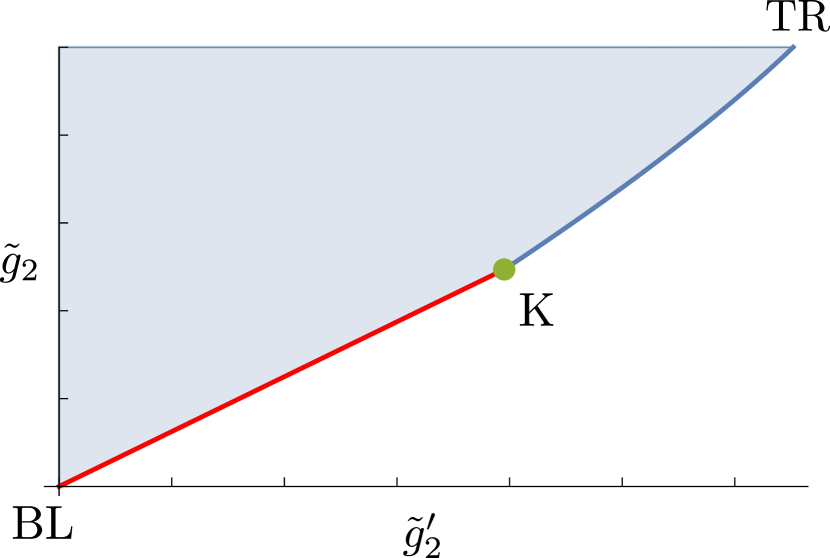
(a) exclusion plot

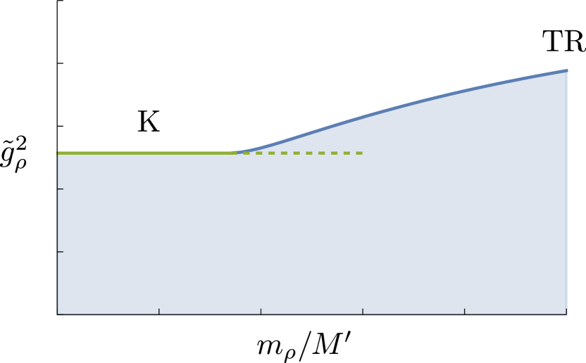
(b) rho coupling plot

Figure 19: Schematic representation of (a) the exclusion plot in the space of four-derivative couplings and (b) the upper bound on the rho coupling. Matching colors should be identified; i.e. the kink (K) on the left corresponds to the plateau on the right and the counterpart of the bound above the kink in (a) is the smooth blue curve in (b), both extending to the top-right corners (TR) of the plots, which are identified.

We start with the case $M^{\prime}/m_{\rho}=1$, when there is no gap above the rho. The amplitude that saturates the bound on the rho coupling at this point is the very same $M_{su-\text{pole}}$ given in (111b). Indeed, its rho coupling is given by

$$\frac{1}{2}g_{\pi\pi\rho}^{2}=\alpha_{J=1}^{(D)}=\, \frac{D}{4}\,{}_{2}F_{1}\left(-\frac{1}{2},1,\frac{D+1}{2},\frac{1}{9}\right)\,\qquad(\text{for }D\geq 3)$$

$$+\, \frac{10-9D}{36}\,{}_{2}F_{1}\left(\frac{1}{2},1,\frac{D+1}{2},\frac{1}{9}\right)\,,$$ (125)

$$\alpha_{J=1}^{(3)}=3\sqrt{2}-4\,,\quad\alpha_{J=0}^{(4)}=3\left(\log 8-2\right)\,,\quad\alpha_{J=0}^{(5)}=8\left(17-12\sqrt{2}\right)\,,\,\dots\,,$$

which, when combined with $g_{1,0}=\frac{1-\alpha_{J=0}^{(D)}}{m^{2}}$, yields (for $D=4$) the normalized coupling

$$\tilde{g}_{\rho}^{2}=\frac{3(\log 8-2)}{1-\log 2}\simeq 0.776674...\,,$$ (126)

in perfect agreement with (96). In the previous section we showed that this simple amplitude rules in the top-right corner (TR) of the exclusion plot, so we learn that the top-right corners of both plots in figure 19 must be identified.

As we increase the gap after the rho by raising $M^{\prime}/m_{\rho}$, we start moving down the blue line of the rho coupling plot. For every value of $M^{\prime}/m_{\rho}$, the amplitude that saturates the bound on $\tilde{g}_{\rho}^{2}$ sits at the top-right corner (TR) of the corresponding plot in figure 13. Since this corner moves down the exclusion plot following closely the original bound, we expect it to match the bound exactly when convergence in $n$ is achieved. Thus, the blue line of figure 19(a) should be identified with the blue line of figure 19(b).

Finally, when $M^{\prime}/m_{\rho}$ is large enough, we reach a plateau in the rho coupling plot that remains constant all the way to $M^{\prime}/m_{\rho}\to\infty$. In the exclusion plot, this happens when the top-right corner (TR) meets the kink (K), where it stops moving. So the kink (K) of figure 19(a) corresponds to the plateau of figure 19(b) (both painted green in the figures). This explains the mysterious relation that we pointed out towards the end of section 5.3: we observed that the value of the plateau in figure 14 for every $n$ matches exactly the position of the corresponding kink on the Skyrme line (given in figure 7). As discussed above, the kink is described very well by a UV completion of the rho with a subtraction at infinity that only changes $g_{1,0}$ by (121). The normalized rho coupling for such an amplitude would be $\tilde{g}_{\rho}^{2}=\frac{1}{3-A}$, which would match exactly the value of $\tilde{g}_{2}$ at the kink (see (122)).

To sum up, the evidence we just presented suggests that the bound above the kink in the exclusion plot corresponds to the upper bound in the right part of the rho coupling plot, while the kink is identified with the plateau. The rho coupling plot thus provides a way to study the bound above the kink of the exclusion plot, which is otherwise hard to study due to its slow convergence in $n$. Our goal for the remainder of this subsection will be to determine what amplitudes saturate the upper bound in the rho coupling plot away from the endpoints.

Our claim is that this bound is saturated by amplitudes with the following spectrum:

1. a fixed rho at the cutoff $m_{\rho}=M$,

2. an infinite tower of higher spins ($J\geq 2$) at the second cutoff $m_{\text{hs}}=M^{\prime}$ combining into

   $$\frac{m_{\text{hs}}^{4}}{(m_{\text{hs}}^{2}-s)(m_{\text{hs}}^{2}-u)}-\alpha_{J=0}^{(D)}M_{\text{spin-0}}-\alpha_{J=1}^{(D)}M_{\text{spin-1}}\,,$$

3. and all higher mesons pushed to infinity.

The first observation is that this spectrum has the correct endpoints. At one end, when $m_{\text{hs}}=m_{\rho}$, the spectrum matches $M_{su-\text{pole}}$; the amplitude at the top-right corner (TR). At the other end, when $m_{\text{hs}}\to\infty$, we are left with a single rho and a bunch of particles at infinity; the spectrum that we identified for the plateau. In between, the upper bound of the rho coupling plot should be covered by tuning $m_{\rho}/m_{\text{hs}}$.

To prove the claim, we just have to redo the rho coupling plot with this more refined spectral assumption and check that we obtain exactly the same bound. If this is the case, this guarantees that there exists at least an amplitude with this spectrum saturating the bound. This plot can be done following the recipe of section 5.3 but adding the explicit contribution from the $su$-pole, i.e. high energy averages should now be shifted by

$$\Big{\langle}F\left(m^{2},J\right)\Big{\rangle}\longrightarrow\frac{1}{2}g_{\pi\pi\rho}^{2}\,F\left(m_{\rho}^{2},J=1\right)+\Big{\langle}F\left(m^{2},J\right)\Big{\rangle}_{su-\text{pole}}+\Big{\langle}F\left(m^{2},J\right)\Big{\rangle}^{\prime\prime}\,,$$ (127)

where $\left<\cdots\right>^{\prime\prime}$ averages over masses above a new cutoff $M^{\prime\prime}>m_{\text{hs}}$ and the relevant averages at the $su$-pole can be derived from

$$\Big{\langle}\frac{\mathcal{P}_{J}(1+\frac{2u}{m^{2}})}{m^{2k}}\Big{\rangle}_{su-\text{pole}} =\frac{-1}{2\pi i}\oint_{m_{\text{hs}}^{2}}ds^{\prime}\,\frac{M(s^{\prime},u)}{s^{\prime k+1}}$$ (128)

$$=\frac{m_{\text{hs}}^{2}}{m_{\text{hs}}^{2}-u}\frac{1}{m_{\text{hs}}^{2k}}-\frac{\alpha_{J=0}^{(D)}}{m_{\text{hs}}^{2k}}-\alpha_{J=1}^{(D)}\frac{\mathcal{P}_{1}\left(1+\frac{2u}{m_{\text{hs}}^{2}}\right)}{m_{\text{hs}}^{2k}}\,.$$

Solving the new dual problem with SDPB sdpb for a fixed $m_{\rho}$ and varying $m_{\text{hs}}\in[m_{\rho},\infty)$ yields an exclusion plot identical to figure 14 (identifying $m_{\text{hs}}=M^{\prime}$). Moreover, the plot is independent of the cutoff $M^{\prime\prime}$; it can be pushed as high as desired and the plot remains the same. This proves our claim; the bound of the rho coupling plot is indeed saturated by an amplitude with the spectrum specified above, and so should be the bound above the kink in the exclusion plot, since we identified them.

6.4 Ruling in (part of) the sliver

With all this information, we can engineer an allowed analytical solution that rules in a larger area than figure 17. Let us discuss it in detail. We start from the $su$-pole amplitude (111b) at a mass $m_{\text{hs}}$ and we remove the spin-one contribution from it. Then, we add the spin-one pole back to the amplitude at a lower mass $m_{\rho}$. Since a bare spin-one amplitude spoils the spin-one Regge behavior, we must use the UV-completed version (119). This is where the masses at infinity become essential. Thus, we consider the amplitude

$$M_{\text{guess}}=M_{su-\text{pole}}(m_{\text{hs}})-\alpha_{J=1}^{(D)}M_{\text{spin-1}}^{(UV)}(m_{\text{hs}})+\lambda\,M_{\text{spin-1}}^{(UV)}(m_{\rho})\,,$$ (129)

where we denote in parentheses the location of the poles (the dependence on $m_{\infty}$ is left implicit). This amplitude depends on a parameter $\lambda$ that in principle could be a function of the masses. From our discussion above we only know $\lambda\to\alpha_{J=1}^{(D)}$ as $m_{\text{hs}}\to m_{\rho}$, but it is otherwise unfixed. We will fix it by demanding that the full amplitude be unitary.

$M_{\text{guess}}$ will be unitary if and only if each of the poles $m_{\rho}$, $m_{\text{hs}}$, $m_{\infty}$ is so (in the sense of (112)). Unitarity at $m_{\rho}$ follows directly from section 6.2 provided that $\lambda\geq 0$. For the pole at $m_{\text{hs}}$, all the coefficients $\gamma_{J}^{(D)}$ are positive except for the $J=0$ one, which is negative. This contribution has its origin in $M_{\text{spin-1}}^{(UV)}(m_{\text{hs}})$ and it dies as $m_{\infty}\to\infty$, but we cannot accept it because we conceptually want $m_{\infty}$ to take large but finite values. Thankfully, we can completely remove this contribution by subtracting $M_{\text{spin-0}}$ with the correct coefficient since $M_{\text{spin-0}}$ alone already has a good Regge behavior. So far, we have seen that $M_{\text{guess}}$ can be made unitary at $m_{\rho}$ and $m_{\text{hs}}$. At the last pole, $m_{\infty}$, the leading term of every coefficient in the limit $m_{\infty}\to\infty$ is proportional to $\gamma_{J}^{(D)}\sim(\lambda-\alpha_{J=1}^{(D)})$ with positive coefficients. So, the negative contributions from $M_{\text{spin-1}}^{(UV)}(m_{\text{hs}})$ can be balanced off by picking $\lambda=\alpha_{J=1}^{(D)}$. This choice is enough to guarantee unitarity as the subleading terms in the limit $m_{\infty}\to\infty$ are positive.

In conclusion, the amplitude

$$M_{\text{final}}=M_{su-\text{pole}}(m_{\text{hs}})-\alpha_{J=1}^{(D)}\left(M_{\text{spin-1}}^{(UV)}(m_{\text{hs}})-\beta_{J=0}^{(D)}M_{\text{spin-0}}(m_{\text{hs}})\right)+\alpha_{J=1}^{(D)}\,M_{\text{spin-1}}^{(UV)}(m_{\rho})$$ (132)

is unitary, crossing-symmetric and spin-one Regge bounded. It is therefore acceptable and we can use it to analytically rule in parts of the space of theories. Its low-energy coefficients (in the limit $m_{\infty}\to\infty$) are

$$M_{\text{final}:}\qquad g_{1,0}\, =\frac{1-\alpha_{0}-3\alpha_{1}}{m_{\text{hs}}^{2}}+\frac{3\alpha_{1}}{m_{\rho}^{2}}\,,\qquad \phantom{\frac{1}{2}}\,\,g_{2,0}=\frac{1-\alpha_{0}-\alpha_{1}}{m_{\text{hs}}^{4}}+\frac{\alpha_{1}}{m_{\rho}^{4}}\,,$$ (133)

$$2g_{2,1}\, =\frac{1-4\alpha_{1}}{m_{\text{hs}}^{4}}+\frac{4\alpha_{1}}{m_{\rho}^{4}}\,, \frac{1}{2}g_{\pi\pi\rho}^{2}=\alpha_{1}\,,$$

where we have adopted a simplified notation for the $\alpha_{J}^{(D)}$ coefficients. The new area ruled in by this amplitude is plotted in figures 20 and 21.

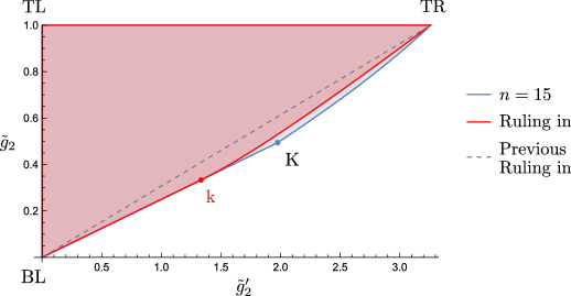
Figure 20: Further ruling in achieved with the amplitude (132). It rules in part of the sliver of figure 17 but there is a bit that still remains.

On the $(\tilde{g}_{2}^{\prime},\tilde{g}_{2})$ plane (figure 20), $M_{\text{final}}$ enlarges the ruled-in region by ruling in part of the sliver of figure 17! The new ruling-in bound splits into two parts as we expected. First, if we keep the rho fixed at the cutoff $m_{\rho}=M$ and we tune $m_{\text{hs}}$, we cover the upper part of the bound (connecting TR to k). This part starts at $m_{\text{hs}}=M$, where the amplitude reduces to $M_{su-\text{pole}}$, and it ends at $m_{\text{hs}}\to\infty$, where it corresponds to $M_{\text{spin-one}}^{(UV)}$. Second, by keeping $m_{\text{hs}}=\infty$ and tuning $m_{\rho}$ we cover the lower segment (connecting k to BL). Unfortunately, there still remains a small part of the sliver to be ruled in, which happens to contain the kink. To push the ruling in up to the kink, one would have to find an amplitude whose low-energy couplings reduce to (122).

On the $(m_{\rho}/M^{\prime},\tilde{g}_{\rho}^{2})$ plane (figure 21), in contrast, the bound is made of just one part, where $m_{\rho}=M$ is fixed and $m_{\text{hs}}(\equiv M^{\prime})\in[M,\infty)$. At the top-right corner (TR), we correctly recover $M_{su-\text{pole}}$, but at the other end we reach $\tilde{g}_{\rho}^{2}=\frac{1}{3}$, corresponding to $M_{\text{spin-1}}^{(UV)}$, which is not quite at the numerical value. In fact, apart from the top-right corner, there is no part of the numerical bound that is saturated by $M_{\text{final}}$, and in particular this simple amplitude does not account for the sharp change in behavior from the curve to the plateau. It would be very interesting to find an amplitude that does so.

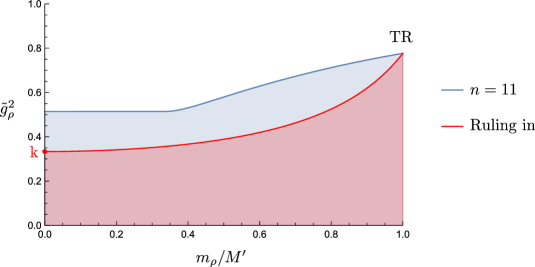
Figure 21: Upper bound on $\tilde{g}_{\rho}^{2}$ ruled in by the amplitude (132), compared to the numerical ruling out at Mandelstam order $n=11$. This amplitude rules in the top-right corner, but it is far from the numerical bound everywhere else.

6.5 A note on the spectrum from SDPB

When trying to identify the spectrum of the theories that saturate our numerical bounds we encountered a technical point that we think is worth mentioning. In principle, one could directly use the results from SDPB to solve for the spectrum numerically. The optimization problem of section 4.1 looks for a “functional” $\vec{\alpha}$ that satisfies $\vec{\alpha}\cdot\vec{v}_{\text{HE}}\left(m^{2},J\right)\geq 0$ for every mass and spin. So, to get the spectrum that saturates the bound one just needs to look for the zeroes of the functional, i.e. solve for the $m^{2}$ and $J$ that make $\vec{\alpha}\cdot\vec{v}_{\text{HE}}\left(m^{2},J\right)$ vanish. However, this procedure generates plots like those of figure 22, which look very different from the spectrum described above. This is somewhat puzzling because theories that saturate a bound are generally expected to be unique.

Figure 22: Spectrum on the bound for representative points (a) below ($\tilde{g}_{2}=0.3$) and (b) above ($\tilde{g}_{2}=0.8$) the kink. Black dots were computed using a 108-dimensional space of functionals whereas for the red dots we used 58-dimensional functionals. For very low spins they seem to have converged, but the dots differ for higher spins.

One possibility is that some of the zeroes might be numerical artifacts such that when they are removed one recovers the spectrum discussed above, and the truth is that the zeroes of the functional do not tell the whole story. To see whether the corresponding particles are relevant in the theory, one has to look at their coupling constants; particles whose couplings are too small effectively drop out. The coupling constant for each pole can be retrieved from SDPB just like one extracts the OPE coefficients in the conformal bootstrap Komargodski:2016auf ; Simmons-Duffin:2016wlq . Doing so reveals that the coupling constants of many points of figure 22 are down by several orders of magnitude, indicating that they might indeed be in some sense spurious and should be removed.

This explanation appears to resolve the mismatch in figure 22(a). The coupling constants in this case are $\sim 10^{-2}$ for the $J=1$ point, $\sim 10^{-5}$ for $J=2$ and $\sim 10^{-9}$ for all other spins. On the other hand, we know that (119) saturates the bound at this point (see figure 20). The spectrum of this amplitude consists of a single rho at a finite mass and everything else pushed to infinity. So, the two spectra match if we disregard all the poles of spin $J>2$ in figure 22(a), which is justified by how small their couplings are.

Similarly, for the spectrum above the kink (figure 22(b)) many zeroes have very small couplings, but even when disregarding them, the spectrum does not quite match our guess from section 6.3. This could be a matter of convergence; that the spectra will match when sufficient null constraints are included, but it could also be that there really is some degeneracy in the solutions that saturate the bound. It is conceivable that more than one theory might yield the same coefficients since, after all, we are first expanding amplitudes at low energies and then projecting down to a two-dimensional slice. The resolution of this puzzle remains unclear to us.

In any case, it has proven useful for figuring out a possible spectrum that saturates the bounds to play with gaps, i.e. recomputing the bound(s) with more detailed spectral assumptions. If the bound gets lower, the assumption was wrong. But if the bound remains the same, we can rest assured that there exists at least an amplitude with that spectrum saturating the bound. Despite the guesswork this involves, we have seen that it provides insight into the geometry of the bounds. It would be interesting to follow this approach for other bounds in the literature like those in Caron-Huot:2020cmc or Caron-Huot:2021rmr (in the latter they found a spectrum from SDPB very similar to figure 22). We expect that similar simplified spectra will be found, which might eventually help us rule in the bounds analytically.

7 Outlook

In this paper we have taken a first step in a systematic program to carve out the space of large $N$ gauge theories. We have focused on the meson sector, assuming that the lowest-lying mesons are massless scalars in the adjoint representation of $SU(N_{f})$, and whose $2\to 2$ scattering amplitude enjoys better than spin-one Regge growth, as would be the case in large $N$ QCD. We have found rigorous two-sided bounds on low-energy EFT parameters.

The exclusion regions display intriguing features, including a tantalizing kink, but we cannot yet decide whether large $N$ QCD sits there. We have managed to “explain” at least a portion of the exclusion boundary in terms of a simple unphysical ansatz for the amplitude (a UV completion of the tree-level rho exchange), but by itself this does not rule out the possibility that large $N$ QCD may sit at the kink. It is perhaps not too far fetched to imagine that if large $N$ QCD is in any sense solvable or integrable, such a conspiracy (i.e. that the contribution of mesons above the rho cancels out in the lowest chiral Lagrangian coefficients) might indeed occur. Another logical possibility is that the kink is indeed unphysical, and that to corner large $N$ QCD one will need to input further physical assumptions. It would be very desirable to have some guidance from large $N$ lattice data.

Clearly this is just the beginning. A natural next step is to consider the full system of $2\to 2$ amplitudes with pions and rhos as external states. In the conformal bootstrap, mixed correlators are essential to zoom in on physical theories, as in the famous example of the tiny island corresponding to the 3D Ising model Kos:2014bka . There is no guarantee that things will work out so beautifully in the large $N$ bootstrap, but we are determined to try. It would also be of interest to see how $1/N$ corrections (which require including low-energy loops in the EFT) affect the geometry of the bounds. The generalization to the glueball sector is of obvious relevance. One would have to deal with the small technical complication that the ligthest states are not massless.

The approach to carving out the space of large $N$ theories illustrated in this paper is very versatile. One can contemplate generalizations to gauge theories in other spacetime dimensions (notably $D=3$), or with different symmetry assumptions. For example, large $N$ confining supersymmetric gauge theories should be a very useful playground.

It is tempting to speculate that there may be some interplay between the spacetime hadronic bootstrap that we have described in this paper, and the conformal bootstrap of the (putative) worldsheet string theory (see Huang:2020nqy for some intriguing ideas in this direction). In a similar vein, it would also be great to make contact with another approach to large $N$ QCD that has been pursued in recent years, based on the 2D EFT on the long string flux tube, see e.g. Aharony:2013ipa ; Dubovsky:2015zey ; Dubovsky:2016cog ; EliasMiro:2019kyf ; EliasMiro:2021nul .

We look forward to explore some of these directions. With some luck, we’ll be able to corner large $N$ QCD or some other theory of physical interest.

Appendix A Internal states in pion scattering

In this appendix we review which mesons can appear as intermediate states in $2\to 2$ pion scattering. Symmetries and conserved quantities impose selection rules that forbid some combinations of quantum numbers for the exchanged mesons. After reviewing the classification of mesons in the quark model, which is exact at large $N$, we derive the selection rules for the scattering of the familiar $SU(2)$ pions. We defer the analysis for general $N_{f}$ to appendix B. Needless to say, the results of this appendix are completely standard – we just apply the conservation laws of strong interactions (reviewed e.g. in meyer ) to the case at hand.

In the quark model mesons are treated as $q\bar{q}$ bound states, and this becomes a rigorous statement at large $N$. As such, they come in irreducible representations of the spin S, the orbital angular momentum L and the total angular momentum $\textbf{J}=\textbf{L}\oplus\textbf{S}$. They are therefore classified by the quantum numbers $S$, $L$, $J=|L-S|,|L-S+1|,\ldots,|L+S|$. In addition, in the chiral limit of vanishing quark masses there is the flavor symmetry $SU(N_{f})$. For $N_{f}=2$, this defines an angular momentum algebra dubbed isospin I. For $N_{f}=3$, there is an additional Cartan generator and therefore states are also labelled by their hypercharge $Y$. For higher $N_{f}$, more quantum numbers appear. Since quarks are in the fundamental representation of the flavor symmetry $\Box$, mesons are classified by the irreducible representations $\Box\otimes\bar{\Box}=\text{adj}\oplus\bullet$. For $SU(2)$, the possibilities are $I=0,1$, i.e. the 1 and the 3. For $SU(3)$, we can have $\textbf{3}\otimes\bar{\textbf{3}}=\textbf{1}\oplus\textbf{8}$. Finally, mesons are also eigenstates of the parity operator P, with eigenvalue

$$P=(-1)^{L+1}\,.$$ (134)

Strong interactions preserve the total angular momentum J, parity P and the $SU(N_{f})$ flavor symmetry. We can use the corresponding conservation laws to constrain the possible quantum numbers for the exchanged states in pion scattering. In general we need the representation theory of $SU(N_{f})$ (developed in appendix B) for this, but one can give an ad hoc derivation of the $SU(2)$ selection rules by defining another symmetry preserved by strong interactions; $G$-parity. G consists of a combination of charge conjugation C and a flip of isospin projection $I_{z}\to-I_{z}$. Only states with $I_{z}=0$ are eigenstates of C, whereas all $SU(2)$ mesons are eigenvalues of G. The eivenvalues of these operators are related to the angular momentum eigenvalues by

$$C =(-1)^{L+S}$$ (135)

$$G =C(-1)^{I}=(-1)^{L+S+I}$$ (136)

We write these eigenvalues as $(I^{G})J^{PC}$. Clearly, not every combination of quantum numbers is allowed. Writing out the possibilities for the angular momenta we find that $J^{++}$ exists for any “spin” $J$; $J^{+-}$ only for odd $J$; $J^{-+}$ only for even $J$ and $J^{--}$ for any $J\neq 0$.

Conventionally, the meson families receive different names depending on their isospin representation, see Table 2. For $SU(2)$ mesons, we only have the first row (corresponding to the 3) and the “prime” of the second row (i.e. the 1). For $SU(3)$, the “prime” is still the 1, but the 8 is made of the first row, the other element in the second row and two copies of the doublet in the third row. This last row contains states with nonvanishing hypercharge (i.e. nonzero strangeness) and $I=\frac{1}{2}$ that are not invariant under G. We denote these states by $(\frac{1}{2})J^{P}$, and their naming convention is $K_{J}$ for $J^{P}=0^{-},1^{+},2^{-},\ldots$ and $K_{J}^{*}$ for $J^{P}=0^{+},1^{-},2^{+},\ldots$.

Table 2: Standard naming convention for the $SU(3)$ (and $SU(2)$) mesons.

$$\begin{array}[]{c||c c c c}(I^{G})J^{PC}&\begin{array}[]{c}S=1\\ L=\text{odd}\\ \forall J\end{array}&\begin{array}[]{c}S=0\\ L=\text{odd}\\ J=\text{odd}\end{array}&\begin{array}[]{c}S=0\\ L=\text{even}\\ J=\text{even}\end{array}&\begin{array}[]{c}S=1\\ L=\text{even}\\ J\neq 0\end{array}\\ \hline\cr\hline\cr I=1&\begin{array}[]{c}a_{J}\\ (1^{-})J^{++}\end{array}&\begin{array}[]{c}b_{J}\\ (1^{+})J^{+-}\end{array}&\begin{array}[]{c}\pi_{J}\\ (1^{-})J^{-+}\end{array}&\begin{array}[]{c}\rho_{J}\\ (1^{+})J^{--}\end{array}\\ \hline\cr I=0&\begin{array}[]{c}f_{J},f^{\prime}_{J}\\ (0^{+})J^{++}\end{array}&\begin{array}[]{c}h_{J},h^{\prime}_{J}\\ (0^{-})J^{+-}\end{array}&\begin{array}[]{c}\eta_{J},\eta^{\prime}_{J}\\ (0^{+})J^{-+}\end{array}&\begin{array}[]{c}\omega_{J},\phi_{J}\\ (0^{-})J^{--}\end{array}\\ \hline\cr I=\frac{1}{2}&\begin{array}[]{c}K_{J}^{*},K_{J}\\ (\frac{1}{2})J^{+}\end{array}&\begin{array}[]{c}K_{J}\\ (\frac{1}{2})J^{+}\end{array}&\begin{array}[]{c}K_{J}\\ (\frac{1}{2})J^{-}\end{array}&\begin{array}[]{c}K_{J}^{*},K_{J}\\ (\frac{1}{2})J^{-}\end{array}\end{array}$$

Selection rules for $SU(2)$

Let us consider $\pi\pi\to\pi\pi$, where the $SU(2)$ pion $\pi$ has quantum numbers $(1^{-})0^{-+}$. For an intermediate state $X$ to appear in this process, the subprocess $\pi\pi\to X$ should be allowed. Or, equivalently, $X$ should be able to decay into two pions. From the conservation laws we learn:

• The pions have $J=0$, so the initial angular momentum must come entirely from the relative angular momentum $\ell$ and $X$ must have “spin” $J=\ell$.

• The initial state can have isospin $1\otimes 1=0\oplus 1\oplus 2$, but there are no single-meson states with isospin $I=2$, so $X$ must have isospin $I=0$ or $1$. This rules out the last row from Table 2.

• Since the initial state has parity $P=(-1)^{2}(-1)^{\ell}$, $X$ must have parity $P=(-1)^{J}$. That is, it can only have positive parity for even spin and negative parity for odd spin. This immediately rules out the two columns at the center of Table 2. In addition, it restricts the possible $J$ for the remaining columns; $J$ must be even in the first column and odd in the last one.

• The $G$-parity of the initial state is fully determined from that of the pions, $G=(-1)(-1)=+1$. We conclude that $X$ must have positive $G$ and therefore the $a_{J}$ and $\omega_{J},\phi_{J}$ families are ruled out.

All in all, we have found that the only mesons that can be exchanged in the $2\to 2$ scattering of $SU(2)$ pions are

$$\left\{\begin{matrix}\rho_{J}&\text{for }J=\text{odd}\;\\ f^{\prime}_{J},(f_{J})&\text{for }J=\text{even}.\end{matrix}\right.$$ (137)

Looking at experimental meson tables PDG we find the first resonances: $f_{0}(500)$, $\rho(700)$, $f_{0}(980)$, $f_{2}(1270)$, etc. However, the current understanding is that the $f_{0}(500)$ (previously known as the $\sigma$) and the $f_{0}(980)$ are not $q\bar{q}$ states but exotic mesons (more precisely, meson-meson resonances) Pelaez:2015qba ; PDG . Thus, at large $N$ the rho (which has spin one) is the first meson exchanged in pion scattering, followed by the $f_{2}(1270)$ (which has spin two).

This discussion concerned the scattering of $SU(2)$ pions embedded in $SU(3)$. When we consider the full scattering of $SU(3)$ “pions” (i.e. including the kaons and the eta), the exchanged families get extended to the full multiplets. In the chiral limit, all the elements in the multiplets should have the same mass, but in nature the $SU(3)$ (and already the $SU(2)$) are explicitly broken by the differences in the masses of the light quarks. We have, for example, that the $a_{2}(1320)$ experimentally shows up at a different mass than the $f_{2}(1270)$.

Appendix B General $N_{f}$

For a general number of flavors, the analog of (9) reads

$${\cal T}=\sum_{{\mathcal{R}}}\mathcal{M}^{{\mathcal{R}}}(s|t,u)\mathbb{P}^{{\mathcal{R}}}_{s}\,,$$ (138)

where the sum runs over the irreps ${\mathcal{R}}\in\text{adj}\otimes\text{adj}$, described in figure 23. The $s$-channel projectors $\mathbb{P}^{{\mathcal{R}}}_{s}$ can be found for example in BandaGuzman:2020wrz and, in terms of the parametrizations of section 2.1, the new amplitudes $\mathcal{M}^{{\mathcal{R}}}(s|t,u)$ are given by

$$\mathcal{M}^{0}(s|t,u)= \,2\frac{N_{f}^{2}-1}{N_{f}}A(s|t,u)+\frac{N_{f}^{2}-2}{N_{f}}\Big{(}A(t|s,u)+A(u|s,t)\Big{)}$$

$$= \,2\frac{N_{f}^{2}-1}{N_{f}}\Big{(}M(s,t)+M(s,u)\Big{)}-\frac{2}{N_{f}}M(t,u)\,,$$ (139a)

$$\mathcal{M}^{\text{adj}_{S}}(s|t,u)= \frac{N_{f}^{2}-4}{N_{f}}A(s|t,u)+\frac{N_{f}^{2}-8}{2N_{f}}\Big{(}A(t|s,u)+A(u|s,t)\Big{)}$$

$$= \,\frac{N_{f}^{2}-4}{N_{f}}\Big{(}M(s,t)+M(s,u)\Big{)}-\frac{4}{N_{f}}M(t,u)\,,$$ (139b)

$$\mathcal{M}^{\text{adj}_{A}}(s|t,u)= \,\frac{N_{f}}{2}\Big{(}A(u|s,t)-A(t|s,u)\Big{)}=N_{f}\Big{(}M(s,u)-M(s,t)\Big{)}\,,$$ (139c)

$$\mathcal{M}^{\bar{s}s}(s|t,u)= \,-\mathcal{M}^{\bar{a}a}(s|t,u)=A(t|s,u)+A(u|s,t)=2M(t,u)\,,$$ (139d)

$$\mathcal{M}^{\bar{s}a}(s|t,u)= \,\mathcal{M}^{\bar{a}s}(s|t,u)=0\,.$$ (139e)

Note that (at large $N$) these amplitudes are not all independent. Also, the reason why the amplitudes in the $\bar{s}a$, $\bar{a}s$ channels vanish exactly is again the single-trace structure of the large $N$ amplitude. The $t\leftrightarrow u$ symmetry of $\mathcal{M}^{{\mathcal{R}}}(s|t,u)$ is related to the symmetrization of the adjoint indices, namely, it is symmetric for ${\mathcal{R}}=0,\text{adj}_{S},\bar{a}a,\bar{s}s$ and antisymmetric for ${\mathcal{R}}=\text{adj}_{A}$. Under $s\leftrightarrow t$, the amplitudes in the different channels mix.

Figure 23: Young tableaux for the $SU(N_{f})$ irreps in the tensor product of two adjoint irreps together with their names. The irreps in the first row come from antisymmetrizing the two adjoint indices while the ones in the second row come from their symmetrization. For $N_{f}=3$, the $\bar{a}a$ does not appear and the decomposition is $\textbf{8}\otimes\textbf{8}=\left(\textbf{10}\oplus\textbf{10}\oplus\textbf{8}\right)_{A}\oplus\left(\textbf{27}\oplus\textbf{8}\oplus\textbf{1}\right)_{S}.$ For $N_{f}=2$, the missing irreps are $\bar{s}a$, $\bar{a}s$, $\bar{a}a$ and $\text{adj}_{S}$, leaving $\textbf{3}\otimes\textbf{3}=\textbf{3}_{A}\oplus\left(\textbf{5}\oplus\textbf{1}\right)_{S}$; the isospin decomposition of section 2.2.

The argument now goes as in the main text. At large $N$, the amplitude $M(s,u)$ is a meromorphic function with poles corresponding to the exchange of physical mesons in the spectrum. Since mesons are exactly $q\bar{q}$ states in this limit, the internal states can only carry irreps appearing in $\Box\otimes\bar{\Box}=\text{adj}\oplus\bullet$. Thus, of the channels of figure 23, the physical intermediate states can only carry the irreps ${\mathcal{R}}=0,\text{adj}_{A},\text{adj}_{S}$. The amplitudes $\mathcal{M}^{\bar{s}s}(s|t,u)$ and $\mathcal{M}^{\bar{a}a}(s|t,u)$ cannot have poles for $s>0$ (at fixed $u<0$). Since both of these amplitudes are proportional to $M(t,u)$, we conclude that the result from section 2.2 generalizes to any $N_{f}$: the basic amplitude $M(s,u)$ (for fixed $u<0$) has poles only on the positive real s axis.

Unitarity

Following section 2.3 we can now expand the ${\mathcal{R}}$-channel amplitudes in partial waves as

$${\rm Im}\,\mathcal{M}^{{\mathcal{R}}}(s|t,u)=s^{\frac{4-D}{2}}\sum_{J}n^{(D)}_{J}\rho^{({\mathcal{R}})}_{J}(s)\,\mathcal{P}_{J}\left(1+\frac{2u}{s}\right)\,,$$ (140)

and demand that each of them be unitary for the full amplitude ${\cal T}_{ab}^{cd}$ to be so. By comparing the symmetry properties of $\mathcal{M}^{{\mathcal{R}}}(s|t,u)$ and the Gegenbauers under $t\leftrightarrow u$ crossing we see that odd spins contribute only to ${\mathcal{R}}=\text{adj}_{A}$ while even spins contribute both to ${\mathcal{R}}=0,\text{adj}_{S}$. Thus, if we expand the basic amplitude in partial waves as in (17) with

$$\rho_{J}(s) =\frac{N_{f}/4}{N_{f}^{2}-1}\rho^{(0)}_{J}(s)=\frac{N_{f}/2}{N_{f}^{2}-4}\rho^{(\text{adj}_{S})}_{J}(s)\qquad s>0\,,\;J\;{\rm even}\,,$$ (141a)

$$\rho_{J}(s) =\frac{1}{2N_{f}}\rho^{(\text{adj}_{A})}_{J}(s)\qquad s>0\,,\;J\;{\rm odd}\,,$$ (141b)

unitarity for the full amplitude implies positivity of $M(s,u)$, just like in (19) but now for any $N_{f}$.

Selection rules

To summarize, from the above discussion we know that at large $N$ and for any $N_{f}$, the even-spin intermediate states in $\pi\pi\to\pi\pi$ scattering can carry any of the irreps ${\mathcal{R}}=0,\text{adj}_{S}$ while odd-spin states must carry ${\mathcal{R}}=\text{adj}_{A}$. From the explicit form of the projectors

$${\mathbb{P}^{(0)}_{s}}_{ab}^{cd}=\frac{1}{N_{f}^{2}-1}\delta_{ab}\delta^{cd}\,,\quad{\mathbb{P}^{(\text{adj}_{S})}_{s}}_{ab}^{cd}=\frac{N_{f}}{N_{f}^{2}-4}d_{abe}d^{cde}\,,\quad{\mathbb{P}^{(\text{adj}_{A})}_{s}}_{ab}^{cd}=\frac{1}{N_{f}}f_{abe}f^{cde}\,,$$ (142)

we learn that the ${\mathcal{R}}=0$ family couples to the pions with a three-point vertex $\sim\delta_{ab}$, the ${\mathcal{R}}=\text{adj}_{A}$ couples with $\sim f_{abc}$ and the ${\mathcal{R}}=\text{adj}_{S}$ with $\sim d_{abc}$. Using

$$f_{abe}f_{cde}=\frac{2}{N_{f}}\Big{(}\delta_{ac}\delta_{bd}-\delta_{ad}\delta_{bc}\Big{)}+d_{ace}d_{bde}-d_{bce}d_{ade}\,,$$ (143)

we see that the exchange of an $\text{adj}_{A}$ alone is enough to generate the group theory factors of (2.1), but neither the $0$ or the $\text{adj}_{S}$ are good on their own. What we need to reproduce the factors from (2.1) in the symmetric side is the sum of both. This means that, at large $N$, the $0$ and the $\text{adj}_{S}$ are degenerate as intermediate states and we always get one when we have the other! Borrowing the parity analysis from appendix A, which still holds, we get that the intermediate states have parity $P=(-1)^{J}$. All in all, for general $N_{f}$ the intermediate states that show up in $\pi\pi\to\pi\pi$ are

$$\left\{\begin{matrix}{\mathcal{R}}=\text{adj}_{A}&\text{ for }J=\text{odd},&P=-\;\\ {\mathcal{R}}=0\oplus\text{adj}_{S}&\text{ for }J=\text{even},&P=+.\end{matrix}\right.$$ (144)

This readily reproduces the results of appendix A, where we derived the $SU(2)$ selection rules. Indeed, for odd $J$ (and negative parity) the internal states form an isospin triplet (${\mathcal{R}}=\text{adj}_{A}$), while for even $J$ (and positive parity) we have the singlet (${\mathcal{R}}=0$). These correspond, respectively to the families $\rho_{J}$ and $f_{J}^{\prime}$. One advantage of this derivation is that it does not rely on $G$-parity. Its role has been taken by the observation that the symmetry of the adjoint indices is related to the parity of $J$. Another obvious advantage of this derivation is its generality. We now see that, indeed, for the scattering of $SU(3)$ pions, the exchanged mesons extend (137) to the whole multiplets: for even $J$ we have all the mesons in the first column of table 2 and for odd $J$ all the mesons in the last column except for the singlet.

References

- (1) G. ’t Hooft, A Planar Diagram Theory for Strong Interactions, Nucl. Phys. B 72 (1974) 461.
- (2) J. M. Maldacena, The Large N limit of superconformal field theories and supergravity, Adv. Theor. Math. Phys. 2 (1998) 231–252, arXiv:hep-th/9711200.
- (3) S. S. Gubser, I. R. Klebanov, and A. M. Polyakov, Gauge theory correlators from noncritical string theory, Phys. Lett. B 428 (1998) 105–114, arXiv:hep-th/9802109.
- (4) E. Witten, Anti-de Sitter space and holography, Adv. Theor. Math. Phys. 2 (1998) 253–291, arXiv:hep-th/9802150.
- (5) A. M. Polyakov, String theory and quark confinement, Nucl. Phys. B Proc. Suppl. 68 (1998) 1–8, arXiv:hep-th/9711002.
- (6) A. M. Polyakov, The Wall of the cave, Int. J. Mod. Phys. A 14 (1999) 645–658, arXiv:hep-th/9809057.
- (7) E. Witten, Baryons in the 1/N Expansion, Nucl. Phys. B 160 (1979) 57–115.
- (8) R. Rattazzi, V. S. Rychkov, E. Tonni, and A. Vichi, Bounding scalar operator dimensions in 4D CFT, JHEP 12 (2008) 031, arXiv:0807.0004 [hep-th].
- (9) D. Poland, S. Rychkov, and A. Vichi, The Conformal Bootstrap: Theory, Numerical Techniques, and Applications, Rev. Mod. Phys. 91 (2019) 015002, arXiv:1805.04405 [hep-th].
- (10) D. Poland and D. Simmons-Duffin, Snowmass White Paper: The Numerical Conformal Bootstrap, in 2022 Snowmass Summer Study. 3, 2022. arXiv:2203.08117 [hep-th].
- (11) S. El-Showk, M. F. Paulos, D. Poland, S. Rychkov, D. Simmons-Duffin, and A. Vichi, Solving the 3D Ising Model with the Conformal Bootstrap, Phys. Rev. D 86 (2012) 025022, arXiv:1203.6064 [hep-th].
- (12) G. Veneziano, Construction of a crossing - symmetric, Regge behaved amplitude for linearly rising trajectories, Nuovo Cim. A 57 (1968) 190–197.
- (13) M. F. Paulos, J. Penedones, J. Toledo, B. C. van Rees, and P. Vieira, The S-matrix bootstrap. Part I: QFT in AdS, JHEP 11 (2017) 133, arXiv:1607.06109 [hep-th].
- (14) M. F. Paulos, J. Penedones, J. Toledo, B. C. van Rees, and P. Vieira, The S-matrix bootstrap II: two dimensional amplitudes, JHEP 11 (2017) 143, arXiv:1607.06110 [hep-th].
- (15) M. F. Paulos, J. Penedones, J. Toledo, B. C. van Rees, and P. Vieira, The S-matrix bootstrap. Part III: higher dimensional amplitudes, JHEP 12 (2019) 040, arXiv:1708.06765 [hep-th].
- (16) Y. He, A. Irrgang, and M. Kruczenski, A note on the S-matrix bootstrap for the 2d O(N) bosonic model, JHEP 11 (2018) 093, arXiv:1805.02812 [hep-th].
- (17) L. Córdova and P. Vieira, Adding flavour to the S-matrix bootstrap, JHEP 12 (2018) 063, arXiv:1805.11143 [hep-th].
- (18) A. Homrich, J. a. Penedones, J. Toledo, B. C. van Rees, and P. Vieira, The S-matrix Bootstrap IV: Multiple Amplitudes, JHEP 11 (2019) 076, arXiv:1905.06905 [hep-th].
- (19) C. Bercini, M. Fabri, A. Homrich, and P. Vieira, S-matrix bootstrap: Supersymmetry, , and symmetry, Phys. Rev. D 101 (2020) 045022, arXiv:1909.06453 [hep-th].
- (20) L. Córdova, Y. He, M. Kruczenski, and P. Vieira, The O(N) S-matrix Monolith, JHEP 04 (2020) 142, arXiv:1909.06495 [hep-th].
- (21) A. Hebbar, D. Karateev, and J. Penedones, Spinning S-matrix bootstrap in 4d, JHEP 01 (2022) 060, arXiv:2011.11708 [hep-th].
- (22) A. L. Guerrieri, A. Homrich, and P. Vieira, Dual S-matrix bootstrap. Part I. 2D theory, JHEP 11 (2020) 084, arXiv:2008.02770 [hep-th].
- (23) Y. He and M. Kruczenski, S-matrix bootstrap in 3+1 dimensions: regularization and dual convex problem, JHEP 08 (2021) 125, arXiv:2103.11484 [hep-th].
- (24) M. Kruczenski, J. Penedones, and B. C. van Rees, Snowmass White Paper: S-matrix Bootstrap, arXiv:2203.02421 [hep-th].
- (25) A. L. Guerrieri, J. Penedones, and P. Vieira, Bootstrapping QCD Using Pion Scattering Amplitudes, Phys. Rev. Lett. 122 (2019) 241604, arXiv:1810.12849 [hep-th].
- (26) A. L. Guerrieri, J. Penedones, and P. Vieira, S-matrix bootstrap for effective field theories: massless pions, JHEP 06 (2021) 088, arXiv:2011.02802 [hep-th].
- (27) G. Veneziano, S. Yankielowicz, and E. Onofri, A model for pion-pion scattering in large-N QCD, JHEP 04 (2017) 151, arXiv:1701.06315 [hep-th].
- (28) B. Lucini and M. Panero, SU(N) gauge theories at large N, Phys. Rept. 526 (2013) 93–163, arXiv:1210.4997 [hep-th].
- (29) T. DeGrand and Y. Liu, Lattice study of large QCD, Phys. Rev. D 94 (2016) 034506, arXiv:1606.01277 [hep-lat]. [Erratum: Phys.Rev.D 95, 019902 (2017)].
- (30) P. Hernández, C. Pena, and F. Romero-López, Large scaling of meson masses and decay constants, Eur. Phys. J. C 79 (2019) 865, arXiv:1907.11511 [hep-lat].
- (31) M. G. Pérez, A. González-Arroyo, and M. Okawa, Meson spectrum in the large limit, JHEP 04 (2021) 230, arXiv:2011.13061 [hep-lat].
- (32) J. Baeza-Ballesteros, P. Hernández, and F. Romero-López, A lattice study of scattering at large , arXiv:2202.02291 [hep-lat].
- (33) S. R. Coleman and E. Witten, Chiral Symmetry Breakdown in Large N Chromodynamics, Phys. Rev. Lett. 45 (1980) 100.
- (34) G. Veneziano, Goldstone Mechanism From Gluon Dynamics, Phys. Lett. B 95 (1980) 90–92.
- (35) A. Martin, Scattering Theory: Unitarity, Analyticity and Crossing, pp. 1–117. Springer Berlin Heidelberg, Berlin, Heidelberg, 1969. https://doi.org/10.1007/BFb0101044.
- (36) T. N. Pham and T. N. Truong, Evaluation of the Derivative Quartic Terms of the Meson Chiral Lagrangian From Forward Dispersion Relation, Phys. Rev. D 31 (1985) 3027.
- (37) B. Ananthanarayan, D. Toublan, and G. Wanders, Consistency of the chiral pion pion scattering amplitudes with axiomatic constraints, Phys. Rev. D 51 (1995) 1093–1100, arXiv:hep-ph/9410302.
- (38) M. R. Pennington and J. Portoles, The Chiral Lagrangian parameters, l1, l2, are determined by the rho resonance, Phys. Lett. B 344 (1995) 399–406, arXiv:hep-ph/9409426.
- (39) J. Comellas, J. I. Latorre, and J. Taron, Constraints on chiral perturbation theory parameters from QCD inequalities, Phys. Lett. B 360 (1995) 109–116, arXiv:hep-ph/9507258.
- (40) P. Dita, Positivity constraints on chiral perturbation theory pion pion scattering amplitudes, Phys. Rev. D 59 (1999) 094007, arXiv:hep-ph/9809568.
- (41) A. Adams, N. Arkani-Hamed, S. Dubovsky, A. Nicolis, and R. Rattazzi, Causality, analyticity and an IR obstruction to UV completion, JHEP 10 (2006) 014, arXiv:hep-th/0602178.
- (42) A. V. Manohar and V. Mateu, Dispersion Relation Bounds for pi pi Scattering, Phys. Rev. D 77 (2008) 094019, arXiv:0801.3222 [hep-ph].
- (43) V. Mateu, Universal Bounds for SU(3) Low Energy Constants, Phys. Rev. D 77 (2008) 094020, arXiv:0801.3627 [hep-ph].
- (44) A. Nicolis, R. Rattazzi, and E. Trincherini, Energy’s and amplitudes’ positivity, JHEP 05 (2010) 095, arXiv:0912.4258 [hep-th]. [Erratum: JHEP 11 (2011) 128].
- (45) D. Baumann, D. Green, H. Lee, and R. A. Porto, Signs of analyticity in single-field inflation, Phys. Rev. D 93 (2016) 023523, arXiv:1502.07304 [hep-th].
- (46) B. Bellazzini, C. Cheung, and G. N. Remmen, Quantum gravity constraints from unitarity and analyticity, Phys. Rev. D 93 (2016) 064076, arXiv:1509.00851 [hep-th].
- (47) B. Bellazzini, Softness and amplitudes’ positivity for spinning particles, JHEP 02 (2017) 034, arXiv:1605.06111 [hep-th].
- (48) C. Cheung and G. N. Remmen, Positive signs in massive gravity, JHEP 04 (2016) 002, arXiv:1601.04068 [hep-th].
- (49) J. Bonifacio, K. Hinterbichler, and R. A. Rosen, Positivity constraints for pseudolinear massive spin-2 and vector Galileons, Phys. Rev. D 94 (2016) 104001, arXiv:1607.06084 [hep-th].
- (50) C. Cheung and G. N. Remmen, Positivity of curvature-squared corrections in gravity, Phys. Rev. Lett. 118 (2017) 051601, arXiv:1608.02942 [hep-th].
- (51) C. de Rham, S. Melville, A. J. Tolley, and S.-Y. Zhou, Positivity bounds for scalar field theories, Phys. Rev. D 96 (2017) 081702, arXiv:1702.06134 [hep-th].
- (52) B. Bellazzini, F. Riva, J. Serra, and F. Sgarlata, Beyond positivity bounds and the fate of massive gravity, Phys. Rev. Lett. 120 (2018) 161101, arXiv:1710.02539 [hep-th].
- (53) C. de Rham, S. Melville, A. J. Tolley, and S.-Y. Zhou, UV complete me: Positivity bounds for particles with spin, JHEP 03 (2018) 011, arXiv:1706.02712 [hep-th].
- (54) C. de Rham, S. Melville, A. J. Tolley, and S.-Y. Zhou, Massive Galileon positivity bounds, JHEP 09 (2017) 072, arXiv:1702.08577 [hep-th].
- (55) K. Hinterbichler, A. Joyce, and R. A. Rosen, Massive spin-2 scattering and asymptotic superluminality, JHEP 03 (2018) 051, arXiv:1708.05716 [hep-th].
- (56) J. Bonifacio, K. Hinterbichler, A. Joyce, and R. A. Rosen, Massive and Massless Spin-2 Scattering and Asymptotic Superluminality, JHEP 06 (2018) 075, arXiv:1712.10020 [hep-th].
- (57) B. Bellazzini, F. Riva, J. Serra, and F. Sgarlata, The other effective fermion compositeness, JHEP 11 (2017) 020, arXiv:1706.03070 [hep-ph].
- (58) J. Bonifacio and K. Hinterbichler, Bounds on amplitudes in effective theories with massive spinning particles, Phys. Rev. D 98 (2018) 045003, arXiv:1804.08686 [hep-th].
- (59) C. de Rham, S. Melville, A. J. Tolley, and S.-Y. Zhou, Positivity bounds for massive spin-1 and spin-2 fields, JHEP 03 (2019) 182, arXiv:1804.10624 [hep-th].
- (60) C. Zhang and S.-Y. Zhou, Positivity bounds on vector boson scattering at the LHC, Phys. Rev. D 100 (2019) 095003, arXiv:1808.00010 [hep-ph].
- (61) B. Bellazzini and F. Riva, New phenomenological and theoretical perspective on anomalous ZZ and Z processes, Phys. Rev. D 98 (2018) 095021, arXiv:1806.09640 [hep-ph].
- (62) B. Bellazzini, M. Lewandowski, and J. Serra, Positivity of amplitudes, weak gravity conjecture, and modified gravity, Phys. Rev. Lett. 123 (2019) 251103, arXiv:1902.03250 [hep-th].
- (63) S. Melville and J. Noller, Positivity in the sky: Constraining dark energy and modified gravity from the UV, Phys. Rev. D 101 (2020) 021502, arXiv:1904.05874 [astro-ph.CO]. [Erratum: Phys. Rev. D 102 (2020) 049902].
- (64) C. de Rham and A. J. Tolley, Speed of gravity, Phys. Rev. D 101 (2020) 063518, arXiv:1909.00881 [hep-th].
- (65) L. Alberte, C. de Rham, A. Momeni, J. Rumbutis, and A. J. Tolley, Positivity constraints on interacting spin-2 fields, JHEP 03 (2020) 097, arXiv:1910.11799 [hep-th].
- (66) L. Alberte, C. de Rham, A. Momeni, J. Rumbutis, and A. J. Tolley, Positivity constraints on interacting pseudo-linear spin-2 fields, JHEP 07 (2020) 121, arXiv:1912.10018 [hep-th].
- (67) Q. Bi, C. Zhang, and S.-Y. Zhou, Positivity constraints on aQGC: carving out the physical parameter space, JHEP 06 (2019) 137, arXiv:1902.08977 [hep-ph].
- (68) G. N. Remmen and N. L. Rodd, Consistency of the Standard Model Effective Field Theory, JHEP 12 (2019) 032, arXiv:1908.09845 [hep-ph].
- (69) G. Ye and Y.-S. Piao, Positivity in the effective field theory of cosmological perturbations, Eur. Phys. J. C 80 (2020) 421, arXiv:1908.08644 [hep-th].
- (70) M. Herrero-Valea, I. Timiryasov, and A. Tokareva, To positivity and beyond, where Higgs-dilaton inflation has never gone before, JCAP 11 (2019) 042, arXiv:1905.08816 [hep-ph].
- (71) B. Bellazzini, J. Elias Miró, R. Rattazzi, M. Riembau, and F. Riva, Positive moments for scattering amplitudes, Phys. Rev. D 104 (2021) 036006, arXiv:2011.00037 [hep-th].
- (72) A. J. Tolley, Z.-Y. Wang, and S.-Y. Zhou, New positivity bounds from full crossing symmetry, JHEP 05 (2021) 255, arXiv:2011.02400 [hep-th].
- (73) S. Caron-Huot and V. Van Duong, Extremal Effective Field Theories, JHEP 05 (2021) 280, arXiv:2011.02957 [hep-th].
- (74) N. Arkani-Hamed, T.-C. Huang, and Y.-T. Huang, The EFT-Hedron, JHEP 05 (2021) 259, arXiv:2012.15849 [hep-th].
- (75) A. Sinha and A. Zahed, Crossing symmetric dispersion relations in quantum field theories, Phys. Rev. Lett. 126 (2021) 181601, arXiv:2012.04877 [hep-th].
- (76) T. Trott, Causality, unitarity and symmetry in effective field theory, JHEP 07 (2021) 143, arXiv:2011.10058 [hep-ph].
- (77) Y.-J. Wang, F.-K. Guo, C. Zhang, and S.-Y. Zhou, Generalized positivity bounds on chiral perturbation theory, JHEP 07 (2020) 214, arXiv:2004.03992 [hep-ph].
- (78) C. Zhang and S.-Y. Zhou, Convex Geometry Perspective on the (Standard Model) Effective Field Theory Space, Phys. Rev. Lett. 125 (2020) 201601, arXiv:2005.03047 [hep-ph].
- (79) C. Zhang, SMEFTs living on the edge: determining the UV theories from positivity and extremality, arXiv:2112.11665 [hep-ph].
- (80) Z.-Z. Du, C. Zhang, and S.-Y. Zhou, Triple crossing positivity bounds for multi-field theories, JHEP 12 (2021) 115, arXiv:2111.01169 [hep-th].
- (81) J. Davighi, S. Melville, and T. You, Natural selection rules: new positivity bounds for massive spinning particles, JHEP 02 (2022) 167, arXiv:2108.06334 [hep-th].
- (82) S. D. Chowdhury, K. Ghosh, P. Haldar, P. Raman, and A. Sinha, Crossing symmetric spinning S-matrix bootstrap: EFT bounds, arXiv:2112.11755 [hep-th].
- (83) J. Henriksson, B. McPeak, F. Russo, and A. Vichi, Rigorous bounds on light-by-light scattering, arXiv:2107.13009 [hep-th].
- (84) Z. Bern, D. Kosmopoulos, and A. Zhiboedov, Gravitational effective field theory islands, low-spin dominance, and the four-graviton amplitude, J. Phys. A 54 (2021) 344002, arXiv:2103.12728 [hep-th].
- (85) S. Caron-Huot, D. Mazac, L. Rastelli, and D. Simmons-Duffin, Sharp Boundaries for the Swampland, JHEP 07 (2021) 110, arXiv:2102.08951 [hep-th].
- (86) X. Li, H. Xu, C. Yang, C. Zhang, and S.-Y. Zhou, Positivity in Multifield Effective Field Theories, Phys. Rev. Lett. 127 (2021) 121601, arXiv:2101.01191 [hep-ph].
- (87) C. de Rham, S. Kundu, M. Reece, A. J. Tolley, and S.-Y. Zhou, Snowmass White Paper: UV Constraints on IR Physics, in 2022 Snowmass Summer Study. 3, 2022. arXiv:2203.06805 [hep-th].
- (88) S. Caron-Huot, Y.-Z. Li, J. Parra-Martinez, and D. Simmons-Duffin, Causality constraints on corrections to Einstein gravity, arXiv:2201.06602 [hep-th].
- (89) J. Henriksson, B. McPeak, F. Russo, and A. Vichi, Bounding Violations of the Weak Gravity Conjecture, arXiv:2203.08164 [hep-th].
- (90) B. Alvarez, J. Bijnens, and M. Sjö, NNLO Positivity Bounds on Chiral Perturbation Theory for a General Number of Flavours, arXiv:2112.04253 [hep-ph].
- (91) A. Bose, A. Sinha, and S. S. Tiwari, Selection rules for the S-Matrix bootstrap, SciPost Phys. 10 (2021) 122, arXiv:2011.07944 [hep-th].
- (92) A. Bose, P. Haldar, A. Sinha, P. Sinha, and S. S. Tiwari, Relative entropy in scattering and the S-matrix bootstrap, SciPost Phys. 9 (2020) 081, arXiv:2006.12213 [hep-th].
- (93) A. Zahed, Positivity and geometric function theory constraints on pion scattering, JHEP 12 (2021) 036, arXiv:2108.10355 [hep-th].
- (94) K. Kawarabayashi and M. Suzuki, Partially conserved axial vector current and the decays of vector mesons, Phys. Rev. Lett. 16 (1966) 255.
- (95) Riazuddin and Fayyazuddin, Algebra of current components and decay widths of rho and K* mesons, Phys. Rev. 147 (1966) 1071–1073.
- (96) E. Witten, Current Algebra Theorems for the U(1) Goldstone Boson, Nucl. Phys. B 156 (1979) 269–283.
- (97) G. Veneziano, U(1) Without Instantons, Nucl. Phys. B 159 (1979) 213–224.
- (98) H. Leutwyler, On the 1/N expansion in chiral perturbation theory, Nucl. Phys. B Proc. Suppl. 64 (1998) 223–231, arXiv:hep-ph/9709408.
- (99) R. Kaiser and H. Leutwyler, Large N(c) in chiral perturbation theory, Eur. Phys. J. C 17 (2000) 623–649, arXiv:hep-ph/0007101.
- (100) M. Correia, A. Sever, and A. Zhiboedov, An Analytical Toolkit for the S-matrix Bootstrap, arXiv:2006.08221 [hep-th].
- (101) R. C. Brower, J. Polchinski, M. J. Strassler, and C.-I. Tan, The Pomeron and gauge/string duality, JHEP 12 (2007) 005, arXiv:hep-th/0603115.
- (102) J. R. Pelaez and F. J. Yndurain, The Pion-pion scattering amplitude, Phys. Rev. D 71 (2005) 074016, arXiv:hep-ph/0411334.
- (103) S. J. Brodsky and G. R. Farrar, Scaling Laws at Large Transverse Momentum, Phys. Rev. Lett. 31 (1973) 1153–1156.
- (104) G. P. Lepage and S. J. Brodsky, Exclusive Processes in Perturbative Quantum Chromodynamics, Phys. Rev. D 22 (1980) 2157.
- (105) S. Caron-Huot, Z. Komargodski, A. Sever, and A. Zhiboedov, Strings from Massive Higher Spins: The Asymptotic Uniqueness of the Veneziano Amplitude, JHEP 10 (2017) 026, arXiv:1607.04253 [hep-th].
- (106) C. Lovelace, A novel application of regge trajectories, Phys. Lett. B 28 (1968) 264–268.
- (107) J. A. Shapiro, Narrow-resonance model with regge behavior for pi pi scattering, Phys. Rev. 179 (1969) 1345–1353.
- (108) M. Bianchi, D. Consoli, and P. Di Vecchia, On the N-pion extension of the Lovelace-Shapiro model, JHEP 03 (2021) 119, arXiv:2002.05419 [hep-th].
- (109) N. Arkani-Hamed, L. Eberhardt, Y.-t. Huang, and S. Mizera, On unitarity of tree-level string amplitudes, JHEP 02 (2022) 197, arXiv:2201.11575 [hep-th].
- (110) J. Gasser and H. Leutwyler, Chiral Perturbation Theory to One Loop, Annals Phys. 158 (1984) 142.
- (111) J. Gasser and H. Leutwyler, Chiral Perturbation Theory: Expansions in the Mass of the Strange Quark, Nucl. Phys. B 250 (1985) 465–516.
- (112) L.-Y. Chiang, Y.-t. Huang, W. Li, L. Rodina, and H.-C. Weng, Into the EFThedron and UV constraints from IR consistency, arXiv:2105.02862 [hep-th].
- (113) Y.-t. Huang, J.-Y. Liu, L. Rodina, and Y. Wang, Carving out the Space of Open-String S-matrix, JHEP 04 (2021) 195, arXiv:2008.02293 [hep-th].
- (114) F. Caracciolo and V. S. Rychkov, Rigorous Limits on the Interaction Strength in Quantum Field Theory, Phys. Rev. D 81 (2010) 085037, arXiv:0912.2726 [hep-th].
- (115) D. Simmons-Duffin, A Semidefinite Program Solver for the Conformal Bootstrap, JHEP 06 (2015) 174, arXiv:1502.02033 [hep-th].
- (116) I. Zahed and G. E. Brown, The Skyrme Model, Phys. Rept. 142 (1986) 1–102.
- (117) E. Witten, Global Aspects of Current Algebra, Nucl. Phys. B 223 (1983) 422–432.
- (118) G. S. Adkins, C. R. Nappi, and E. Witten, Static Properties of Nucleons in the Skyrme Model, Nucl. Phys. B 228 (1983) 552.
- (119) J. Bijnens, G. Colangelo, and J. Gasser, K(l4) decays beyond one loop, Nucl. Phys. B 427 (1994) 427–454, arXiv:hep-ph/9403390.
- (120) L. Girlanda, M. Knecht, B. Moussallam, and J. Stern, Comment on the prediction of two loop standard chiral perturbation theory for low-energy pi pi scattering, Phys. Lett. B 409 (1997) 461–468, arXiv:hep-ph/9703448.
- (121) G. Amoros, J. Bijnens, and P. Talavera, form-factors and scattering, Nucl. Phys. B 585 (2000) 293–352, arXiv:hep-ph/0003258. [Erratum: Nucl.Phys.B 598, 665–666 (2001)].
- (122) P. Haldar, A. Sinha, and A. Zahed, Quantum field theory and the Bieberbach conjecture, SciPost Phys. 11 (2021) 002, arXiv:2103.12108 [hep-th].
- (123) P. Raman and A. Sinha, QFT, EFT and GFT, JHEP 12 (2021) 203, arXiv:2107.06559 [hep-th].
- (124) G. Ecker, J. Gasser, A. Pich, and E. de Rafael, The Role of Resonances in Chiral Perturbation Theory, Nucl. Phys. B 321 (1989) 311–342.
- (125) J. F. Donoghue, C. Ramirez, and G. Valencia, The Spectrum of QCD and Chiral Lagrangians of the Strong and Weak Interactions, Phys. Rev. D 39 (1989) 1947.
- (126) M. Bando, T. Kugo, S. Uehara, K. Yamawaki, and T. Yanagida, Is rho Meson a Dynamical Gauge Boson of Hidden Local Symmetry?, Phys. Rev. Lett. 54 (1985) 1215.
- (127) M. Bando, T. Kugo, and K. Yamawaki, Nonlinear Realization and Hidden Local Symmetries, Phys. Rept. 164 (1988) 217–314.
- (128) Z. Komargodski, Vector Mesons and an Interpretation of Seiberg Duality, JHEP 02 (2011) 019, arXiv:1010.4105 [hep-th].
- (129) J. J. Sakurai, Currents and mesons. Chicago U.P., 1969.
- (130) J. J. Sakurai, Eight Ways of Determining the rho-Meson Coupling Constant, Phys. Rev. Lett. 17 (1966) 1021–1024.
- (131) Particle Data Group Collaboration, P. A. Zyla et al., Review of Particle Physics, PTEP 2020 (2020) 083C01.
- (132) Z. Komargodski and D. Simmons-Duffin, The Random-Bond Ising Model in 2.01 and 3 Dimensions, J. Phys. A 50 (2017) 154001, arXiv:1603.04444 [hep-th].
- (133) D. Simmons-Duffin, The Lightcone Bootstrap and the Spectrum of the 3d Ising CFT, JHEP 03 (2017) 086, arXiv:1612.08471 [hep-th].
- (134) F. Kos, D. Poland, and D. Simmons-Duffin, Bootstrapping Mixed Correlators in the 3D Ising Model, JHEP 11 (2014) 109, arXiv:1406.4858 [hep-th].
- (135) O. Aharony and Z. Komargodski, The Effective Theory of Long Strings, JHEP 05 (2013) 118, arXiv:1302.6257 [hep-th].
- (136) S. Dubovsky and V. Gorbenko, Towards a Theory of the QCD String, JHEP 02 (2016) 022, arXiv:1511.01908 [hep-th].
- (137) S. Dubovsky and G. Hernandez-Chifflet, Yang–Mills Glueballs as Closed Bosonic Strings, JHEP 02 (2017) 022, arXiv:1611.09796 [hep-th].
- (138) J. Elias Miró, A. L. Guerrieri, A. Hebbar, J. a. Penedones, and P. Vieira, Flux Tube S-matrix Bootstrap, Phys. Rev. Lett. 123 (2019) 221602, arXiv:1906.08098 [hep-th].
- (139) J. Elias Miró and A. Guerrieri, Dual EFT bootstrap: QCD flux tubes, JHEP 10 (2021) 126, arXiv:2106.07957 [hep-th].
- (140) C. A. Meyer, Light and exotic mesons, in Hadronic Structure, 14’th Annual HUGS at CEBAF. 2001.
- (141) J. R. Pelaez, From controversy to precision on the sigma meson: a review on the status of the non-ordinary resonance, Phys. Rept. 658 (2016) 1, arXiv:1510.00653 [hep-ph].
- (142) V. M. Banda Guzmán, R. Flores-Mendieta, J. Hernández, and F. d. J. Rosales-Aldape, Spin and flavor projection operators in the spin-flavor group, Phys. Rev. D 102 (2020) 036010, arXiv:2006.14169 [hep-ph].