Focal Modulation Networks

Abstract

We propose focal modulation networks (FocalNets in short), where self-attention (SA) is completely replaced by a focal modulation module for modeling token interactions in vision. Focal modulation comprises three components: $(i)$ focal contextualization, implemented using a stack of depth-wise convolutional layers, to encode visual contexts from short to long ranges, $(ii)$ gated aggregation to selectively gather contexts into a modulator for each query token, and $(iii)$ element-wise affine transformation to inject the modulator into the query. Extensive experiments show FocalNets exhibit extraordinary interpretability (Fig. 1) and outperform the SoTA SA counterparts (e.g., Swin and Focal Transformers) with similar computational cost on the tasks of image classification, object detection, and segmentation. Specifically, FocalNets with tiny and base size can achieve 82.3% and 83.9% top-1 accuracy on ImageNet-1K. After pretrained on ImageNet-22K in 224² resolution, it attains 86.5% and 87.3% top-1 accuracy when finetuned with resolution 224² and 384², respectively. For object detection with Mask R-CNN [29], FocalNet base trained with 1$\times$ outperforms the Swin counterpart by 2.1 points and already surpasses Swin trained with 3$\times$ schedule (49.0 v.s. 48.5). For semantic segmentation with UPerNet [90], FocalNet base at single-scale outperforms Swin by 2.4, and beats Swin at multi-scale (50.5 v.s. 49.7). Using large FocalNet and Mask2former [13], we achieve 58.5 mIoU for ADE20K semantic segmentation, and 57.9 PQ for COCO Panoptic Segmentation. Using huge FocalNet and DINO [106], we achieved 64.3 and 64.4 mAP on COCO minival and test-dev, respectively, establishing new SoTA on top of much larger attention-based models like Swinv2-G [53] and BEIT-3 [84]. These encouraging results render focal modulation is probably what we need for vision.

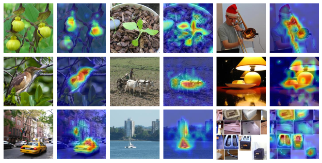
Figure 1: Given images, Focal Modulation Network (FocalNet) exhibits extraordinary interpretability – the modulation automatically and gradually converge on the object regions that induce the recognition categories. NO visual explanation tools like CAM [117] or Grad-CAM [61] are used.

1 Introduction

Transformers [79], originally proposed for natural language processing (NLP), have become a prevalent architecture in computer vision since the seminal work of Vision Transformer (ViT) [22]. Its promise has been demonstrated in various vision tasks including image classification [75, 82, 89, 54, 108, 78], object detection [3, 120, 114, 18], segmentation [80, 86, 14], and beyond [45, 112, 4, 9, 81, 41]. In Transformers, the self-attention (SA) is arguably the key to its success which enables input-dependent global interactions, in contrast to convolution operation which constrains interactions in a local region with a shared kernel. Despite this advantages, the efficiency of SA has been a concern due to its quadratic complexity over the number of visual tokens, especially for high-resolution inputs. To address this, many works have proposed SA variants through token coarsening [82], window attention [54, 78, 108], dynamic token selection [60, 98, 59], or the hybrid [95, 15]. Meanwhile, a number of models have been proposed by augmenting SA with (depth-wise) convolutions to capture long-range dependencies with a good awareness of local structures [89, 25, 94, 23, 21, 40, 7, 20].

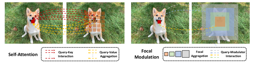
Figure 2: Illustrative comparison between (window-wise) Self-Attention (SA) [79, 22, 54] and our proposed Focal Modulation. Given the query token   and target tokens (  ,$\cdots$, ), SA first performs query-key interactions to compute the attention scores, and then query-value aggregations to capture the context from other tokens. In contrast, Focal Modulation first encodes spatial context at different levels of granularity into modulators (   ,   ,  ,  ), which are then adaptively injected into the query token in a query-dependent manner. Clearly, SA requires heavy interaction and aggregation operations, while our Focal Modulation reverses their order and turn both of them light-weight. Figures better viewed in color.

In this work, we aim at answering the fundamental question: Is there a better way than SA to model input-dependent long-range interactions? We start with an analysis on the current advanced designs for SA. In Fig. 2 left side, we show a commonly-used (window-wise) attention between the red query token and its surrounding orange tokens proposed in ViTs [22] and Swin Transformer [54]. To produce the outputs, SA involve heavy query-key interactions (red arrows) followed by equally heavy query-value aggregations (yellow arrows) between the query and a large number of spatially distributed tokens (context features). However, is it necessary to undertake such heavy interactions and aggregations? In this work, we take an alternative way by first aggregating contexts focally around each query and then adaptively modulating the query with the aggregated context. As shown in Fig. 2 right side, we can simply apply query-agnostic focal aggregations (e.g., depth-wise convolution) to generate summarized tokens at different levels of granularity. Afterwards, these summarized tokens are adaptively aggregated into a modulator, which is finally injected into the query.

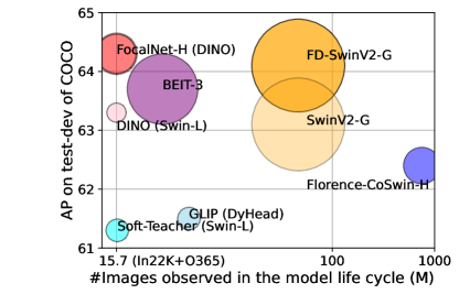
Figure 3: Comparison with SoTA on COCO object detection. Circle size indicates the model size.

This alteration still enables input-dependent token interaction, but significantly eases the process by decoupling the aggregation from individual queries, hence making the interactions light-weight upon merely a couple of features. Our method is inspired by focal attention [95] which performs multiple levels of aggregation to capture fine- and coarse-grained visual contexts. However, our method extracts at each query position the modulator and exploits a much simpler way for the query-modulator interaction. We call this new mechanism Focal Modulation, with which we replace SA to build an attention-free architecture, Focal Modulation Network, or FocalNet in short.

Finally, extensive experiments on image classification, object detection and segmentation, show our FocalNets consistently and significantly outperform the SoTA SA counterparts with comparable costs. Notably, our FocalNet achieves 82.3% and 83.9% top-1 accuracy using tiny and base model size, but with comparable and doubled throughput than Swin and Focal Transformer, respectively. When pretrained on ImageNet-22K with $224^{2}$ resolution, our FocalNets achieve 86.5% and 87.3% in $224^{2}$ and $384^{2}$ resolution, respectively, which are comparable or better than Swin at similar cost. The advantage is particularly significant when transferred to dense prediction tasks. For object detection on COCO [49], our FocalNets with tiny and base model size achieve 46.1 and 49.0 box mAP on Mask R-CNN 1$\times$, surpassing Swin with 3$\times$ schedule (46.0 and 48.5 box mAP). For semantic segmentation on ADE20k [118], our FocalNet with base model size achieves 50.5 mIoU at single-scale evaluation, outperforming Swin at multi-scale evaluation (49.7 mIoU). Using the pretrained large FocalNet, we achieve 58.5 mIoU for ADE20K semantic segmentation, and 57.9 PQ for COCO Panoptic Segmentation based on Mask2former [12]. Using huge FocalNet and DINO [106], we achieved 64.3 and 64.4 mAP on COCO minival and test-dev, respectively, establishing new SoTA on COCO over much larger attention-based models like Swinv2-G [53] and BEIT-3 [84]. Please find the visual comparison in Figure 3, and details in the experiments. Finally, we apply our Focal Modulation in monolithic layout as ViTs and clearly demonstrate its superiority across different model sizes.

2 Related Work

Self-attentions. Transformer [79] is first introduced to vision in Vision Transformer (ViT) [22] by splitting an image into a sequence of visual tokens. The self-attention (SA) strategy in ViTs has demonstrated superior performance to modern convolutional neural networks (ConvNets) such as ResNet [30] when trained with optimized recipes [22, 75]. Afterwards, multi-scale architectures [5, 82, 94], light-weight convolution layers [89, 25, 46], local self-attention mechanisms [54, 108, 15, 95] and learnable attention weights [101] have been proposed to boost the performance and support high-resolution input. More comprehensive surveys are covered in [38, 27, 38]. Our focal modulation significantly differs from SA by first aggregating the contexts from different levels of granularity and then modulating individual query tokens, rendering an attention-free mechanism for token interactions. For context aggregation, our method is inspired by focal attention proposed in [95]. However, the context aggregation for focal modulation is performed at each query location instead of target locations, followed by a modulation rather than an attention. These differences in mechanism lead to significant improvement of efficiency and performance. Another closely related work is Poolformer [100] which uses a pooling to summarize the local context and a simple subtraction to adjust the individual inputs. Despite decent efficiency, it lags behind popular vision transformers like Swin on performance. As we will show, capturing local structures at different levels is essential.

MLP architectures. Visual MLPs can be categorized into two groups: $(i)$ Global-mixing MLPs, such as MLP-Mixer [72] and ResMLP [74], perform global communication among visual tokens through spatial-wise projections augmented by various techniques, such as gating, routing, and Fourier transforms [51, 58, 70, 71]. $(ii)$ Local-mixing MLPs sample nearby tokens for interactions, using spatial shifting, permutation, and pseudo-kernel mixing [99, 32, 48, 8, 26]. Recently, Mix-Shift-MLP [113] exploits both local and global interactions with MLPs, in a similar spirit of focal attention [95]. Both MLP architectures and our focal modulation network are attention-free. However, focal modulation with multi-level context aggregation naturally captures the structures in both short- and long-range, and thus achieves much better accuracy-efficiency trade-off.

Convolutions. ConvNets have been the primary driver of the renaissance of deep neural networks in computer vision. The field has evolved rapidly since the emerge of VGG [63], InceptionNet [67] and ResNet [30]. Representative works that focus on the efficiency of ConvNets are MobileNet [33], ShuffleNet [111] and EfficientNet [69]. Another line of works aimed at integrating global context to compensate ConvNets such as SE-Net [35], Non-local Network [85], GCNet [2], LR-Net [34] and C3Net [97], etc. Introducing dynamic operation is another way to augment ConvNets as demonstrated in Involution [43] and DyConv [10]. Recently, ConvNets strike back from two aspects: $(i)$ convolution layers are integrated to SA and bring significant gains [89, 25, 46, 23] or the vice versa [76]; $(ii)$ ResNets have closed the gap to ViTs using similar data augmentation and regularization strategies [88], and replacing SA with (dynamic) depth-wise convolution [28, 55] can also slightly surpass Swin. Our focal modulation network also exploits depth-wise convolution as the micro-architecture but goes beyond by introducing a multi-level context aggregation and input-dependent modulation. We will show this new module significantly outperforms raw convolution networks.

3 Focal Modulation Network

3.1 From Self-Attention to Focal Modulation

Given a visual feature map ${{\bf X}}\in\mathbb{R}^{H\times W\times C}$ as input, a generic encoding process generates for each visual token (query) $\boldsymbol{x}_{i}\in\mathbb{R}^{C}$ a feature representation $\boldsymbol{y}_{i}\in\mathbb{R}^{C}$ via the interaction $\mathcal{T}$ with its surroundings ${{\bf X}}$ (e.g., neighboring tokens) and aggregation $\mathcal{M}$ over the contexts.

Self-attention. The self-attention modules use a late aggregation procedure formulated as

$$\small\boldsymbol{y}_{i}=\mathcal{M}_{1}(\mathcal{T}_{1}(\boldsymbol{x}_{i},{{\bf X}}),{{\bf X}}),$$ (1)

where the aggregation $\mathcal{M}_{1}$ over the contexts ${{\bf X}}$ is performed after the attention scores between query and target are computed via interaction $\mathcal{T}_{1}$.

Focal modulation. In contrast, Focal Modulation generates refined representation $\boldsymbol{y}_{i}$ using an early aggregation procedure formulated as

$$\small\boldsymbol{y}_{i}=\mathcal{T}_{2}(\mathcal{M}_{2}(i,{{\bf X}}),\boldsymbol{x}_{i}),$$ (2)

where the context features are first aggregated using $\mathcal{M}_{2}$ at each location $i$, then the query interacts with the aggregated feature based on $\mathcal{T}_{2}$ to form $\boldsymbol{y}_{i}$.

Comparing Eq. (1) and Eq. (2), we see that $(i)$ the context aggregation of Focal Modulation $\mathcal{M}_{2}$ amortizes the computation of contexts via a shared operator (e.g., depth-wise convolution), while $\mathcal{M}_{1}$ in SA is more computationally expensive as it requires summing over non-shareable attention scores for different queries; $(ii)$ the interaction $\mathcal{T}_{2}$ is a lightweight operator between a token and its context, while $\mathcal{T}_{1}$ involves computing token-to-token attention scores, which has quadratic complexity.

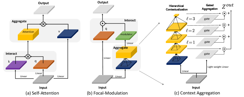
Figure 4: Left: Comparing SA (a) and Focal Modulation (b) side by side. Right: Detailed illustration of context aggregation in Focal Modulation (c).

Based on Eq. (2), we instantiate our Focal Modulation to

$$\boldsymbol{y}_{i}=q(\boldsymbol{x}_{i})\odot m(i,{{\bf X}}),$$ (3)

where $q(\cdot)$ is a query projection function and $\odot$ is the element-wise multiplication. $m(\cdot)$ is a context aggregation function, whose output is called modulator. Fig. 4(a) and (b) compare Self-Attention and Focal Modulation. The proposed Focal Modulation has the following favorable properties:

• Translation invariance. Since $q(\cdot)$ and $m(\cdot)$ are always centered at the query token $i$ and no positional embedding is used, the modulation is invariant to translation of input feature map ${{\bf X}}$.

• Explicit input-dependency. The modulator is computed via $m(\cdot)$ by aggregating the local features around target location $i$, hence our Focal Modulation is explicitly input-dependent.

• Spatial- and channel-specific. The target location $i$ as a pointer for $m(\cdot)$ enables spatial-specific modulation. The element-wise multiplication enables channel-specific modulation.

• Decoupled feature granularity. $q(\cdot)$ preserve the finest information for individual tokens, while $m(\cdot)$ extracts the coarser context. They are decoupled but combined through modulation.

In what follows, we describe in detail the implementation of $m(\cdot)$ in Eq. (3).

3.2 Context Aggregation via $m(\cdot)$

It has been proved that both short- and long-range contexts are important for visual modeling [95, 21, 55]. However, a single aggregation with larger receptive field is not only computationally expensive in time and memory, but also undermines the local fine-grained structures which are particularly useful for dense prediction tasks. Inspired by [95], we propose a multi-scale hierarchical context aggregation. As depicted in Fig. 4 (c), the aggregation procedure consists of two steps: hierarchical contextualization to extract contexts from local to global ranges at different levels of granularity and gated aggregation to condense all context features at different granularity levels into the modulator.

Step 1: Hierarchical Contextualization.

Given input feature map ${{\bf X}}$, we first project it into a new feature space with a linear layer ${\bf Z}^{0}=f_{z}({{\bf X}})\in\mathbb{R}^{H\times W\times C}$. Then, a hierarchical presentation of contexts is obtained using a stack of $L$ depth-wise convolutions. At focal level $\ell\in\{1,...,L\}$, the output ${\bf Z}^{\ell}$ is derived by:

$$\small{\bf Z}^{\ell}=f_{a}^{\ell}({\bf Z}^{\ell-1})\triangleq\textsf{GeLU}(\textsf{DWConv}({\bf Z}^{\ell-1}))\in\mathbb{R}^{H\times W\times C},$$ (4)

where $f_{a}^{\ell}$ is the contextualization function at the $\ell$-th level, implemented via a depth-wise convolution DWConv with kernel size $k^{\ell}$ followed by a GeLU activation function [31]. The use of depth-wise convolution for hierarchical contextualization of Eq. (4) is motivated by its desirable properties. Compared to pooling [100, 35], depth-wise convolution is learnable and structure-aware. In contrast to regular convolution, it is channel-wise and thus computationally much cheaper.

Hierarchical contextualization of Eq. (4) generates $L$ levels of feature maps. At level $\ell$, the effective receptive field is $r^{\ell}=1+\sum_{i=1}^{\ell}(k^{\ell}-1)$, which is much larger than the kernel size $k^{\ell}$. To capture global context of the whole input, which could be high-resolution, we apply a global average pooling on the $L$-th level feature map ${\bf Z}^{L+1}=\textsf{Avg-Pool}({\bf Z}^{L})$. Thus, we obtain in total $(L+1)$ feature maps $\{{\bf Z}^{\ell}\}_{\ell=1}^{L+1}$, which collectively capture short- and long-range contexts at different levels of granularity.

Step 2: Gated Aggregation.

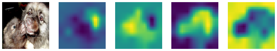
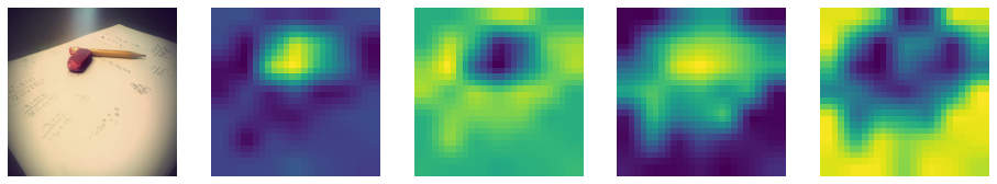
Figure 5: Visualization of gating values ${{\bf G}}$ in Eq. (5) at last layer of our FocalNet ($L=3$) pretrained on ImageNet-1K. The columns from left to right are input images, gating maps at focal level 1,2,3 and global level.

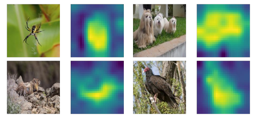
Figure 6: Visualization of modulator values (corresponding to the right side of $\odot$ in Eq. (6)) at the last layer in FocalNet. The original modulator map is upsampled for display.

In this step, the $(L+1)$ feature maps obtained via hierarchical contextualization are condensed into a modulator. In an image, the relation between a visual token (query) and its surrounding contexts often depends on the content itself. For example, the model might rely on local fine-grained features for encoding the queries of salient visual objects, but mainly global coarse-grained features for the queries of background scenes. Based on this intuition, we use a gating mechanism to control how much to aggregate from different levels for each query. Specifically, we use a linear layer to obtain a spatial- and level-aware gating weights ${\bf G}=f_{g}({{\bf X}})\in\mathbb{R}^{H\times W\times(L+1)}$. Then, we perform a weighted sum through an element-wise multiplication to obtain a single feature map ${\bf Z}^{out}$ which has the same size as the input ${{\bf X}}$,

$$\small{\bf Z}^{out}=\sum_{\ell=1}^{L+1}{\bf G}^{\ell}\odot{\bf Z}^{\ell}\in\mathbb{R}^{H\times W\times C}$$ (5)

where ${\bf G}^{\ell}\in\mathbb{R}^{H\times W\times 1}$ is a slice of ${\bf G}$ for the level $\ell$. When visualizing these gating maps in Fig. 6, we surprisingly find our FocalNet indeed learns gathering the context from different focal levels adaptively as we expect. As we can see, for a token on a small object, it focuses more on the fine-grained local structure at low focal level, while a token in a uniform background needs to be aware of much larger contexts from higher levels. Until now, all the aggregation is spatial. To enable the communication across different channels, we use another linear layer $h(.)$ to obtain the modulator map ${\bf M}=h({\bf Z}^{out})\in\mathbb{R}^{H\times W\times C}$. In Fig. 6, we visualize the magnitude of modulator ${\bf M}$ at the last layer of our FocalNet. Interestingly, the modulators automatically pay more attention to the objects inducing the category, which implies a simple way of interpreting FocalNets.

Focal Modulation.

Given the implementation of $m(\cdot)$ as described above, Focal Modulation of Eq.(3) can be rewritten at the token level as

$$\boldsymbol{y}_{i}=q(\boldsymbol{x}_{i})\odot h(\sum_{\ell=1}^{L+1}{\boldsymbol{g}}^{\ell}_{i}\cdot\boldsymbol{z}^{\ell}_{i})$$ (6)

where ${\boldsymbol{g}}_{i}^{\ell}$ and $\boldsymbol{z}_{i}^{\ell}$ are the gating value and visual feature at location $i$ of ${\bf G}^{\ell}$ and ${\bf Z}^{\ell}$, respectively. We summarize the proposed Focal Modulation in Pytorch-style pseudo code in Algorithm 1, which is implemented with a few depth-wise convolution and linear layers.

1

# Input/output shape: (B, H, W, C); Batchsize B; Feature map height H, width W, dim C

# Focal levels: L; Conv kernel size at level $\ell$: k^ℓ

2

3def init( ):

4       pj_in, pj_cxt = Linear(C, 2*C + (L+1)), Conv2d(C, C, 1)

5       hc_layers = [Sequential(Conv2d(C, C, k^ℓ, groups=C), GeLU()) for $\ell$ in range(L)]

6       pj_out = Sequential(Linear(C, C), Dropout())

7      

8

9def forward(x, m=0):

10       x = pj_in(x).permute(0, 3, 1, 2)

11       q, z, gate = split(x, (C, C, L+1), 1)

12      

13      for $\ell$ in range(L):

14             z = hc_layers[$\ell$](z)               # Eq.(4), hierarchical contextualization

15             m = m + z * gate[:, $\ell$:$\ell$+1]  # Eq.(5), gated aggregation

16      m = m + GeLU(z.mean(dim=(2,3))) * gate[:,L:]

17      x = q * pj_cxt(m)                          # Eq.(6), Focal Modulation

18       return pj_out( x.permute(0, 2, 3, 1) )

19

Algorithm 1 Pseudo code for Focal Modulation.

3.3 Relation to Other Architecture Designs

Based on the formula in Eq. (6), we build the connections between our Focal Modulation and other relevant architecture designs beyond Self-Attention.

Depth-wise Convolution has been used to augment the local structural modeling for SA [89, 21, 25] or purely to enable efficient long-range interactions [33, 28, 55]. Our Focal Modulation also employs depth-wise convolution as one of the building blocks. However, instead of using its response as the output directly, our Focal Modulation uses depth-wise convolution to capture the hierarchical contexts, which are then converted into modulator to modulate each query. As we will show in our experiments, these three components as a whole contribute the final decent performance.

Squeeze-and-Excitation (SE) was proposed in [35] prior to the emerge of vision transformers. It exploits a global average pooling to squeeze the context globally, and then a multi-layer perception (MLP) followed by a Sigmoid to obtain the excitation scalar for each channel. SE can be considered as a special case of Focal Modulation. Setting $L=0$ in Eq. (6), Focal Modulation degrades to $q(\boldsymbol{x}_{i})\odot h(f_{g}(\boldsymbol{x}_{i})\cdot\textsf{Avg-Pool}(f_{z}({{\bf X}})))$ which resembles SE. In our experiments, we study this variant and find that a global context is far insufficient for visual modeling.

PoolFormer was recently introduced in [100], and draw many attentions due to its simplicity. It uses average pooling to extract the context locally in a sliding-window, and then adjust the query tokens using an element-wise subtraction. It shares similar spirit to SE-Net, but uses local context instead of global ones, and subtraction instead of multiplication. Putting it and Focal Modulation side-by-side, we can find both of them extract the local context and enable the query-context interaction but in different ways (Pooling v.s. Convolution, Subtraction v.s. Modulation).

3.4 Complexity

In Focal Modulation as Eq. (6), there are mainly three linear projections $q(\cdot)$, $h(\cdot)$, and $f_{z}(\cdot)$ for ${\bf Z}^{0}$. Besides, it requires a lightweight linear function $f_{g}(\cdot)$ for gating and $L$ depth-wise convolution $f_{a}^{\{1,...,L\}}$ for hierarchical contextualization. Therefore, the overall number of learnable parameters is $3C^{2}+C(L+1)+C\sum_{\ell}(k^{\ell})^{2}$. Since $L$ and $(k^{\ell})^{2}$ are typically much smaller than $C$, the model size is mainly determined by the first term as we will show in Sec. 4. Regarding the time complexity, besides the linear projections and the depth-wise convolution layers, the element-wise multiplications introduce $\mathcal{O}(C(L+2))$ for each visual token. Hence, the total complexity for a feature map is $\mathcal{O}(HW\times(3C^{2}+C(2L+3)+C\sum_{\ell}(k^{\ell})^{2}))$. For comparison, a window-wise attention in Swin Transformer with window size $w$ is $\mathcal{O}(HW\times(3C^{2}+2Cw^{2}))$, while a vanilla self-attention in ViTs takes $\mathcal{O}((HW)^{2}C+HW\times(3C^{2}))$.

3.5 Network Architectures

We use the same stage layouts and hidden dimensions as in Swin [54] and Focal Transformers [95], but replace the SA modules with the Focal Modulation modules. We thus construct a series of Focal Modulation Network (FocalNet) variants. In FocalNets, we only need to specify the number of focal levels ($L$) and the kernel size ($k^{\ell}$) at each level. For simplicity, we gradually increase the kernel size by 2 from lower focal levels to higher ones, i.e., $k^{\ell}=k^{\ell-1}+2$. To match the complexities of Swin and Focal Transformers, we design a small receptive field (SRF) and a large receptive field (LRF) version for each of the four layouts by using 2 and 3 focal levels, respectively. We use non-overlapping convolution layers for patch embedding at the beginning (kernel size=$4\times 4$, stride=4) and between two stages (kernel size=$2\times 2$, stride=2), respectively.

4 Experiment

4.1 Image Classification

We compare different methods on ImageNet-1K classification [19]. Following the recipes in [75, 54, 95], we train FocalNet-T, FocalNet-S and FocalNet-B with ImageNet-1K training set and report Top-1 accuracy (%) on the validation set. Training details are described in the appendix.

To verify the effectiveness of FocalNet, we compare it with three groups of methods based on ConvNets, Transformers and MLPs. The results are reported in Table 4. We see that FocalNets outperform the conventional CNNs (e.g., ResNet [30] and the augmented version [88]), MLP architectures such as MLP-Mixer [73] and gMLP [50], and Transformer architectures DeiT [75] and PVT [82]. In particular, we compare FocalNets against Swin and Focal Transformers which use the same architecture to verify FocalNet’s stand-alone effectiveness at the bottom part. We see that FocalNets with small receptive fields (SRF) achieve consistently better performance than Swin Transformer but with similar model size, FLOPs and throughput. For example, the tiny FocalNet improves Top-1 accuracy by $0.9\%$ over Swin-Tiny. To compare with Focal Transformers (FocalAtt), we change to large receptive fields (LRF) though it is still much smaller than the one used in FocalAtt. Focal modulation outperforms the strong and sophisticatedly designed focal attention across all model sizes. More importantly, its run-time speed is much higher than FocalAtt by getting rid of many time-consuming operations like rolling and unfolding.

Model augmentation. We investigate whether some commonly used techniques for vision transformers can also improve our FocalNets. First, we study the effect of using overlapped patch embedding for downsampling [25]. Following [89], we change the kernel size and stride from $(4,4)$ to $(7,4)$ for patch embedding at the beginning, and $(2,2)$ to $(3,2)$ for later stages. The comparisons are reported in Table 4. Overlapped patch embedding improves the performance for models of all sizes, with slightly increased computational complexity and time cost. Second, we make our FocalNets deeper but thinner as in [21, 119]. In Table 4, we change the depth layout of our FocalNet-T from 2-2-6-2 to 3-3-16-3, and FocalNet-S/B from 2-2-18-2 to 4-4-28-4. Meanwhile, the hidden dimension at first stage is reduced from 96, 128 to 64, 96, respectively. These changes lead to smaller model sizes and fewer FLOPs, but higher time cost due to the increased number of sequential blocks. It turns out that going deeper improves the performance of FocalNets significantly. These results demonstrate that the commonly used model augmentation techniques developed for vision transformers can be easily adopted to improve the performance of FocalNets.

Model	#Params. (M)	FLOPs (G)	Throughput (imgs/s)	Top-1 (%)
ResNet-50 [30]	25.0	4.1	1294	76.2
ResNet-101 [30]	45.0	7.9	745	77.4
ResNet-152 [30]	60.0	11.0	522	78.3
ResNet-50-SB [88]	25.0	4.1	1294	79.8
ResNet-101-SB [88]	45.0	7.9	745	81.3
ResNet-152-SB [88]	60.0	11.6	522	81.8
DW-Net-T [28]	24.2	3.8	1030	81.2
DW-Net-B [28]	74.3	12.9	370	83.2
Mixer-B/16 [73]	59.9	12.7	455	76.4
gMLP-S [50]	19.5	4.5	785	79.6
gMLP-B [50]	73.4	15.8	301	81.6
ResMLP-S24 [74]	30.0	6.0	871	79.4
ResMLP-B24 [74]	129.1	23.0	61	81.0
DeiT-Small/16 [75]	22.1	4.6	939	79.9
DeiT-Base/16 [75]	86.6	17.5	291	81.8
PVT-Small [82]	24.5	3.8	794	79.8
PVT-Medium [82]	44.2	6.7	517	81.2
PVT-Large [82]	61.4	9.8	352	81.7
PoolFormer-m36 [100]	56.2	8.8	463	82.1
PoolFormer-m48 [100]	73.5	11.6	347	82.5
Swin-Tiny [54]	28.3	4.5	760	81.2
FocalNet-T (SRF)	28.4	4.4	743	82.1
Swin-Small [54]	49.6	8.7	435	83.1
FocalNet-S (SRF)	49.9	8.6	434	83.4
Swin-Base [54]	87.8	15.4	291	83.5
FocalNet-B (SRF)	88.1	15.3	280	83.7
FocalAtt-Tiny [95]	28.9	4.9	319	82.2
FocalNet-T (LRF)	28.6	4.5	696	82.3
FocalAtt-Small	51.1	9.4	192	83.5
FocalNet-S (LRF)	50.3	8.7	406	83.5
FocalAtt-Base [95]	89.8	16.4	138	83.8
FocalNet-B (LRF)	88.7	15.4	269	83.9

Table 1: ImageNet-1K classification comparison.

Model	Overlapped PatchEmbed	#Params. (M)	FLOPs (G)	Throughput (imgs/s)	Top-1 (%)
FocalNet-T (SRF)		28.4	4.4	743	82.1
FocalNet-T (SRF)	✓	30.4	4.4	730	82.4
FocalNet-S (SRF)		49.9	8.6	434	83.4
FocalNet-S (SRF)	✓	51.8	8.6	424	83.4
FocalNet-B (SRF)		88.1	15.3	286	83.7
FocalNet-B (SRF)	✓	91.6	15.3	278	84.0

Table 2: Effect of overlapped patch embedding.

Model	Depth	Dim.	#Params.	FLOPs	Throughput	Top-1
FocalNet-T (SRF)	2-2-6-2	96	28.4	4.4	743	82.1
FocalNet-T (SRF)	3-3-16-3	64	25.1	4.0	663	82.7
FocalNet-S (SRF)	2-2-18-2	96	49.9	8.6	434	83.4
FocalNet-S (SRF)	4-4-28-4	64	38.2	6.4	440	83.5
FocalNet-B (SRF)	2-2-18-2	128	88.1	15.3	280	83.7
FocalNet-B (SRF)	4-4-28-4	96	85.1	14.3	247	84.1

Table 3: Effect of deeper and thinner networks.

Model	Img. Size	#Params	FLOPs	Throughput	Top-1
ResNet-101x3 [30]	3842	388.0	204.6	-	84.4
ResNet-152x4 [30]	4802	937.0	840.5	-	85.4
ViT-B/16 [22]	3842	86.0	55.4	99	84.0
ViT-L/16 [22]	3842	307.0	190.7	30	85.2
Swin-Base [54]	2242/2242	88.0	15.4	291	85.2
FocalNet-B	2242/2242	88.1	15.3	280	85.6
Swin-Base [54]	3842/3842	88.0	47.1	91	86.4
FocalNet-B	2242/3842	88.1	44.8	94	86.5
Swin-Large [54]	2242/2242	196.5	34.5	155	86.3
FocalNet-L	2242/2242	197.1	34.2	144	86.5
Swin-Large [54]	3842/3842	196.5	104.0	49	87.3
FocalNet-L	2242/3842	197.1	100.6	50	87.3

Table 4: ImageNet-1K finetuning results with models pretrained on ImageNet-22K. Numbers before and after “/” are resolutions used for pretraining and finetuning, respectively.

ImageNet-22K pretraining. We investigate the effectiveness of FocalNets when pretrained on ImageNet-22K which contains 14.2M images and 21K categories. Training details are described in the appendix. We report the results in Table 4. Though FocalNet-B/L are both pretrained with $224\times 224$ resolution and directly transferred to target domain with $384\times 384$ image size, we can see that they consistently outperform Swin Transformers.

4.2 Language-Image Contrast Learning

We also study FocalNet in the recently popular language-image contrastive learning paradigm. More specifically, our experiment setting follows the Academic Track of the Image Classification in the Wild (ICinW) Challenge, where ImageNet-21K (ImageNet-1K images are removed), GCC3M+12M and YFCC15M are used in pre-training, and 20 downstream datasets and ImageNet-1K are evaluated to report the zero-shot performance [42]. This setting was originally proposed in UniCL [96]. We pre-train the model with the UniCL objective, and the vision backbone is specified as FocalNet-B and Swin-B for comparisons. The results are reported in Table 5. FocalNet-B outperforms Swin-B by 0.8 averaged gain on 20 datasets in ICinW and 2.0 gain on ImageNet-1K, respectively.

Dataset		Caltech101	CIFAR10	CIFAR100	Country211	DescriTextures	EuroSAT	FER2013	FGVC Aircraft	Food101	GTSRB	HatefulMemes	KITTI	MNIST	Oxford Flowers	Oxford Pets	PatchCamelyon	Rendered SST2	RESISC45	Stanford Cars	VOC2007	Mean Acc.	ImageNet-1K
Swin-B		84.0	93.0	69.5	7.3	25.5	24.4	30.4	2.7	71.0	9.0	52.6	12.4	10.1	70.4	52.4	50.6	50.1	44.8	13.8	81.3	43.2	52.2
FocalNet-B		84.8	90.2	67.8	6.7	25.4	35.3	30.8	3.5	68.3	11.1	51.0	17.9	11.3	71.7	44.9	52.1	49.5	41.4	24.2	81.3	44.0	54.2
Gains		0.9	-2.7	-1.7	-0.6	-0.1	11.0	0.5	0.8	-2.7	2.1	-1.6	5.5	1.2	1.3	-7.6	1.6	-0.6	-3.4	10.5	0.0	+0.8	2.0

Table 5: Zero-shot performance comparison of FocalNet-B and Swin-B on ELEVATER benchmark [42]. We calculate the gains marked in green for positive results. The mean score over 20 datasets and the top-1 accuracy on ImageNet-1K are reported in the last two columns, respectively.

4.3 Detection and Segmentation

Object detection and instance segmentation. We make comparisons on object detection with COCO 2017 [49]. We choose Mask R-CNN [29] as the detection method and use FocalNet-T/S/B pretrained on ImageNet-1K as the backbones. All models are trained on the 118k training images and evaluated on 5K validation images. We use two standard training recipes, $1\times$ schedule with 12 epochs and $3\times$ schedule with 36 epochs. Following [54], we use the same multi-scale training strategy by randomly resizing the shorter side of an image to $[480,800]$. Similar to [95], we increase the kernel size $k^{\ell}$ by 6 for context aggregation at all focal levels to adapt to higher input resolutions. Instead of up-sampling the relative position biases as in [95], FocalNets uses simple zero-padding for the extra kernel parameters. This expanding introduces negligible overhead but helps extract longer range contexts. For training, we use AdamW [57] as the optimizer with initial learning rate $10^{-4}$ and weight decay $0.05$. All models are trained with batch size 16. We set the stochastic drop rates to $0.1$, $0.2$, $0.3$ in $1\times$ and $0.3$, $0.5$, $0.5$ in $3\times$ training schedule for FocalNet-T/S/B, respectively.

The results are shown in Table 6. We measure both box and mask mAP, and report the results for both small and large receptive field models. Comparing with Swin Transformer, FocalNets improve the box mAP (AP^b) by $2.2$, $1.5$ and $1.9$ in $1\times$ schedule for tiny, small and base models, respectively. In $3\times$ schedule, the improvements are still consistent and significant. Remarkably, the $1\times$ performance of FocalNet-T/B (45.9/48.8) rivals Swin-T/B (46.0/48.5) trained with $3\times$ schedule. When comparing with FocalAtt [95], FocalNets with large receptive fields consistently outperform under all settings and cost much less FLOPs. For instance segmentation, we observe the similar trend as that of object detection for FocalNets. To further verify the generality of FocalNets, we train three detection models, Cascade Mask R-CNN [1], Sparse RCNN [66] and ATSS [109] with FocalNet-T as the backbone. We train all models with $3\times$ schedule, and report the box mAPs in Table 8. As we can see, FocalNets bring clear gains to all three detection methods over the previous SoTA methods.

Backbone	#Params	FLOPs	Mask R-CNN 1x						Mask R-CNN 3x
	(M)	(G)	$AP^{b}$	$AP^{b}_{50}$	$AP^{b}_{75}$	$AP^{m}$	$AP^{m}_{50}$	$AP^{m}_{75}$	$AP^{b}$	$AP^{b}_{50}$	$AP^{b}_{75}$	$AP^{m}$	$AP^{m}_{50}$	$AP^{m}_{75}$
ResNet50 [30]	44.2	260	38.0	58.6	41.4	34.4	55.1	36.7	41.0	61.7	44.9	37.1	58.4	40.1
PVT-Small[82]	44.1	245	40.4	62.9	43.8	37.8	60.1	40.3	43.0	65.3	46.9	39.9	62.5	42.8
Twins-SVT-S [15]	44.0	228	43.4	66.0	47.3	40.3	63.2	43.4	46.8	69.2	51.2	42.6	66.3	45.8
Swin-Tiny [54]	47.8	264	43.7	66.6	47.7	39.8	63.3	42.7	46.0	68.1	50.3	41.6	65.1	44.9
FocalNet-T (SRF)	48.6	267	45.9(+2.2)	68.3	50.1	41.3	65.0	44.3	47.6(+1.6)	69.5	52.0	42.6	66.5	45.6
FocalAtt-Tiny [95]	48.8	291	44.8	67.7	49.2	41.0	64.7	44.2	47.2	69.4	51.9	42.7	66.5	45.9
FocalNet-T (LRF)	48.9	268	46.1(+1.3)	68.2	50.6	41.5	65.1	44.5	48.0(+0.8)	69.7	53.0	42.9	66.5	46.1
ResNet101 [30]	63.2	336	40.4	61.1	44.2	36.4	57.7	38.8	42.8	63.2	47.1	38.5	60.1	41.3
ResNeXt101-32x4d [92]	62.8	340	41.9	62.5	45.9	37.5	59.4	40.2	44.0	64.4	48.0	39.2	61.4	41.9
PVT-Medium [82]	63.9	302	42.0	64.4	45.6	39.0	61.6	42.1	44.2	66.0	48.2	40.5	63.1	43.5
Twins-SVT-B [15]	76.3	340	45.2	67.6	49.3	41.5	64.5	44.8	48.0	69.5	52.7	43.0	66.8	46.6
Swin-Small [54]	69.1	354	46.5	68.7	51.3	42.1	65.8	45.2	48.5	70.2	53.5	43.3	67.3	46.6
FocalNet-S (SRF)	70.8	356	48.0(+1.5)	69.9	52.7	42.7	66.7	45.7	48.9(+0.4)	70.1	53.7	43.6	67.1	47.1
FocalAtt-Small [95]	71.2	401	47.4	69.8	51.9	42.8	66.6	46.1	48.8	70.5	53.6	43.8	67.7	47.2
FocalNet-S (LRF)	72.3	365	48.3(+0.9)	70.5	53.1	43.1	67.4	46.2	49.3(+0.5)	70.7	54.2	43.8	67.9	47.4
ResNeXt101-64x4d [92]	102.0	493	42.8	63.8	47.3	38.4	60.6	41.3	44.4	64.9	48.8	39.7	61.9	42.6
PVT-Large[82]	81.0	364	42.9	65.0	46.6	39.5	61.9	42.5	44.5	66.0	48.3	40.7	63.4	43.7
Twins-SVT-L [15]	119.7	474	45.9	-	-	41.6	-	-	-	-	-	-	-	-
Swin-Base [54]	107.1	497	46.9	69.2	51.6	42.3	66.0	45.5	48.5	69.8	53.2	43.4	66.8	46.9
FocalNet-B (SRF)	109.4	496	48.8(+1.9)	70.7	53.5	43.3	67.5	46.5	49.6(+1.1)	70.6	54.1	44.1	68.0	47.2
FocalAtt-Base [95]	110.0	533	47.8	70.2	52.5	43.2	67.3	46.5	49.0	70.1	53.6	43.7	67.6	47.0
FocalNet-B (LRF)	111.4	507	49.0(+1.2)	70.9	53.9	43.5	67.9	46.7	49.8(+0.8)	70.9	54.6	44.1	68.2	47.2

Table 6: COCO object detection and instance segmentation results with Mask R-CNN [29].

Method	Backbone	#Param.	FLOPs	$AP^{b}$	$AP^{b}_{50}$	$AP^{b}_{75}$
C. Mask R-CNN [1]	R-50 [30]	82.0	739	46.3	64.3	50.5
	DW-Net-T [28]	82.0	730	49.9	68.6	54.3
	Swin-T [54]	85.6	742	50.5	69.3	54.9
	FocalNet-T (SRF)	86.4	746	51.5	70.1	55.8
	FocalAtt-T [95]	86.7	770	51.5	70.6	55.9
	FocalNet-T (LRF)	87.1	751	51.5	70.3	56.0
Sparse R-CNN [66]	R-50 [30]	106.1	166	44.5	63.4	48.2
	Swin-T [54]	109.7	172	47.9	67.3	52.3
	FocalNet-T (SRF)	110.5	172	49.6	69.1	54.2
	FocalAtt-T [95]	110.8	196	49.0	69.1	53.2
	FocalNet-T (LRF)	111.2	178	49.9	69.6	54.4
ATSS [109]	R-50 [30]	32.1	205	43.5	61.9	47.0
	Swin-T [54]	35.7	212	47.2	66.5	51.3
	FocalNet-T (SRF)	36.5	215	49.2	68.1	54.2
	FocalAtt-T [95]	36.8	239	49.5	68.8	53.9
	FocalNet-T (LRF)	37.2	220	49.6	68.7	54.5

Table 7: A comparison of models with different object detection methods, trained using the $3\times$ schedule.

Backbone	Crop Size	#Param.	FLOPs	mIoU	+MS
ResNet-101 [30]	512	86	1029	44.9	-
Twins-SVT-L [15]	512	133	-	48.8	50.2
DW-Net-T [28]	512	56	928	45.5	-
DW-Net-B [28]	512	132	924	48.3	-
Swin-T [54]	512	60	941	44.5	45.8
FocalNet-T (SRF)	512	61	944	46.5	47.2
FocalAtt-T [95]	512	62	998	45.8	47.0
FocalNet-T (LRF)	512	61	949	46.8	47.8
Swin-S [54]	512	81	1038	47.6	49.5
FocalNet-S (SRF)	512	83	1035	49.3	50.1
FocalAtt-S [95]	512	85	1130	48.0	50.0
FocalNet-S (LRF)	512	84	1044	49.1	50.1
Swin-B [54]	512	121	1188	48.1	49.7
FocalNet-B (SRF)	512	124	1180	50.2	51.1
FocalAtt-B [95]	512	126	1354	49.0	50.5
FocalNet-B (LRF)	512	126	1192	50.5	51.4

Table 8: Semantic segmentation on ADE20K [118]. All models are trained with UperNet [90]. MS means multi-scale evaluation.

Semantic Segmentation. We benchmark FocalNets on semantic segmentation, a dense prediction task that requires fine-grained understanding and long-range interactions. We use ADE20K [118] for our experiments and follow [54] to use UperNet [90] as the segmentation method. With FocalNet-T/S/B trained on ImageNet-1K as the backbones, we train UperNet for 160k iterations with input resolution $512\times 512$ and batch size 16. For comparisons, we report both single- and multi-scale (MS) mIoU. Table 8 shows the results with different backbones. FocalNet outperforms Swin and Focal Transformer significantly under all settings. Even for the base models, FocalNet (SRF) exceeds Swin Transformer by $2.1$ and $1.4$ at single- and multi-scale, respectively. Compared with Focal Transformer, FocalNets outperform Focal Transformer, with a larger gain than that of Swin Transformer, and consume much less FLOPs. These results demonstrate the superiority of FocalNets on the pixel-level dense prediction tasks, in addition to the instance-level object detection task.

Backbone	Method	#Param	mIoU	+MS
HRNet-w48 [65]	OCRNet [103]	71M	45.7	-
ResNeSt-200 [105]	DLab.v3+ [6]	88M	48.4	-
Swin-B [54]	UperNet [90]	121M	48.1	49.7
Twins-SVT-L [15]	UperNet [90]	133M	48.8	50.2
MiT-B5 [91]	SegFormer [91]	85M	51.0	51.8
ViT-L/16† [22]	SETR [115]	308M	50.3	-
Swin-L† [54]	UperNet [90]	234M	52.1	53.5
ViT-L/16† [22]	Segmenter [64]	334M	51.8	53.6
Swin-L† [54]	K-Net [110]	-	-	54.3
Swin-L† [54]	PatchDiverse [24]	234M	53.1	54.4
VOLO-D5 [101]	UperNet [90]	-	-	54.3
Focal-L†	UperNet [90]	240M	54.0	55.4
CSwin-L†	UperNet [90]	208M	54.0	55.7
BEIT-L†	UperNet [90]	441M	56.7	57.0
Swinv2-G‡ [52]	UperNet [90]	>3.0B	59.1	-
ViT-Adapter-L† [11]	Mask2Former [12]	568M	58.3	59.0
Swin-L†	Mask2Former [12]	216M	56.4	57.7
Swin-L-FaPN†	Mask2Former [12]	-	56.1	57.3
Swin-L-SeMask† [37]	Mask2Former [12]	-	57.0	58.2
FocalNet-L† (Ours)	Mask2Former [12]	218M	57.3	58.5

Table 9: Systematic comparisons of semantic segmentation on ADE20K validation set. ^† indicates pretraining with ImageNet-22K and ^‡ means using extra data additionally.

Backbone	Method	#Param.	PQ	AP	mIoU
ResNet-50 [30]	DETR [3]	-	43.4	-	-
ResNet-50 [30]	K-Net [110]	-	47.1	-	-
ResNet-50 [30]	Panoptic SegFormer [47]	47M	50.0	-	-
ResNet-50 [30]	Mask2Former [12]	44M	51.9	41.7	62.4
PVTv2-B5 [83]	Panoptic SegFormer [47]	101M	54.1	-	-
Swin-T [54]	MaskFormer [14]	42M	47.7	33.6	60.4
Swin-B [54]	MaskFormer [14]	102M	51.1	37.8	62.6
Swin-T [54]	Mask2Former [12]	47M	53.2	43.3	63.2
Swin-B [54]	Mask2Former [12]	107M	55.1	45.2	65.1
Swin-L$\dagger$ [54]	MaskFormer [14]	212M	52.7	40.1	64.8
Swin-L$\dagger$ [54]	Panoptic SegFormer [47]	-	55.8	-	-
Swin-L$\dagger$ [54]	Mask2Former [14] (200 queries)	216M	57.8	48.6	67.4
FocalNet-L$\dagger$ (Ours)	Mask2Former [14] (200 queries)	226M	57.9	48.4	67.3

Table 10: Panoptic segmentation on COCO [49]. $\dagger$ means pretraining with ImageNet-22K. All models evaluated on minival with single-scale. PQ, AP and mIoU are three metrics for measuring the panoptic segmentation, instance segmentation and semantic segmentation, respectively.

Method	#Params.	Backbone Pretraining	Detection Pretraining	W/ Mask	val2017		test-dev
					w/o TTA	w/ TTA	w/o TTA	w/ TTA
Swin-L (HTC++) [54]	284M	IN-22K (14M)	n/a	✓	57.1	58.0	57.7	58.7
DyHead (Swin-L) [17]	213M	IN-22K (14M)	n/a	✓	56.2	58.4	-	-
Focal-L (DyHead) [95]	229M	IN-22K (14M)	n/a	✓	56.4	58.7	-	58.9
Soft-Teacher (Swin-L) [93]	284M	IN-22K (14M)	COCO-unlabeled + O365	✓	60.1	60.7	-	61.3
GLIP (DyHead) [44]	$\geq$284M	IN-22K (14M)	FourODs + GoldG + Cap24M	✗	-	60.8	-	61.5
Florence-CoSwin-H [102]	$\geq$637M	FLD-900M (900M)	FLD-9M	✗	-	62.0	-	62.4
SwinV2-G [52]	3.0B	In-22K + ext-70M (84M)	O365	✓	61.9	62.5	-	63.1
DINO (Swin-L) [106]	218M	IN-22K (14M)	O365	✗	63.1	63.2	63.2	63.3
BEIT-3 [84]	1.9B	IN-22K + Image-Text Pairs (35M) + Text (160GB)	O365	✓	-	-	-	63.7
FD-SwinV2-G [87]	3.0B	IN-22K + IN-1K + ext-70M (85M)	O365	✓	-	-	-	64.2
FocalNet-H (DINO)	746M	IN-22K (14M)	O365	✗	64.0	64.2	64.1	64.4

Table 11: Comparisons of best detection models on COCO across the leaderboard. “W/ Mask” means whether using mask annotations for finetuning on COCO. “TTA” means test-time-augmentation. “FLD-900M” used in Florence [102] contains 900M free-form image-text pairs. “ex-70M” used in Swinv2 [52] is a private classification dataset containing 70M images.

Scaling-up FocalNets.

Given the superior results for FocalNets on object detection and segmentation shown above, we further investigate its effectiveness while scaling up. Particularly, to fairly compare with Swin-L pretrained on ImageNet-22K with 384$\times$384, we also pretrain our FocalNet-L on ImageNet-22K with 384$\times$384 with 3 focal levels and kernel sizes $[3,5,7]$. We use Mask2former [12] for semantic segmentation on ADE20K and panoptic segmentation on COCO. As shown in Table 10, FocalNet-L achieves superior performance to Swin-L with similar model size and same pretraining data. We note that the methods in gray font like Swinv2-G and ViT-Adapter-L achieve better performance but use much more parameters and training data. In Table 10, we compare different models for panoptic segmentation on COCO with 133 categories. Our FocalNet-L slightly outperforms Swin-L on PQ. These results clearly demonstrate the effectiveness of our FocalNets for various segmentation tasks when being scaled up to large model size.

Finally, we study the effectiveness of our FocalNets for object detection at scale. Currently, many methods scaled to billions of model parameters [52, 84]. To catch up, we pretrain a huge FocalNet with around 700M parameters on ImageNet-22K for 90 epochs using the same regime used for our large models. On top of the pretrained FocalNet-H, we use the public available object detection method DINO [106]. Following previous works, we pretrain the detection model on Object365 [62], and finetune it on COCO training set. We report the results in Table 11. Our model beats the SoTA methods like SwinV2-G [52], BEIT-3 [106], while consuming much less parameters and backbone pretraining data. It also outperforms the SwinV2-G tuned with the new feature distillation technique [87], and establishes a new SoTA on the COCO leaderboard. We believe our FocalNet can be further boosted after equipping the same technique and being pretrained on more data.

4.4 Network Inspection

Model Variants. We compare in Table 12 six different model variants derived from FocalNet.

• Depth-wise ConvNet. It feeds the feature vectors at the top level $L$ to a two-layer MLP. The resultant model is close to DW-Net [28]. Although it can achieve 81.6%, surpassing Swin (81.3%), it underperforms FocalNet by 0.7%. FocalNet uses depth-wise convolutions as a component but differently for aggregating contexts, which is then used to modulate each individual tokens.

• Pooling Aggregator. It replaces the depth-wise convolution module with average pooling, and is similar to MetaFormer [100] in terms of token aggregation. Average pooling has slightly lower complexity but leads to a significant drop of accuracy by 1.8%. Compared with depth-wise convolution, pooling is permutation-invariant and thus incapable of capturing visual structures.

• Global Pooling Aggregator. It removes local aggregations at all levels and only keeps the global one (${\bf Z}^{L+1}$). This variant resembles SENet [35]. It turns out that global context alone is insufficient for visual modeling, leading to a significant 6.7% drop.

• Multi-scale Self-Attention. Given the summarized tokens at different levels, a straightforward way to combine them is performing a SA among all of them. We have developed two SA methods: computing $q,k,v$ before and after aggregation, respectively. Both methods result in visible performance drop and increase the run time latency, compared to FocalNet.

• Sliding-window Self-Attention. Finally, we apply a sliding-window SA for each visual token within a window. Since it involves dense interactions for each fine-grained tokens, the time and memory cost explodes, and the performance is worse than FocalNet.

Model	Formula	#Param.	FLOPs	Throughput	Top-1
FocalNet-T (LRF)	$\boldsymbol{y}_{i}=q(\boldsymbol{x}_{i})\odot h(\sum_{\ell=1}^{L+1}{\boldsymbol{g}}^{\ell}_{i}\cdot\boldsymbol{z}^{\ell}_{i})$	28.6	4.49	696	82.3
$\rightarrow$ Depth-width ConvNet	$\boldsymbol{y}_{i}=q(\textsf{GeLU}(h(\boldsymbol{z}^{L}_{i})))$	28.6	4.47	738	81.6 (-0.7)
$\rightarrow$ Pooling Aggregator	$\boldsymbol{y}_{i}=q(\boldsymbol{x}_{i})\odot h(\sum_{\ell=1}^{L+1}{\boldsymbol{g}}^{\ell}_{i}\cdot\textsf{Avg-Pool}(\boldsymbol{z}^{\ell-1}_{i}))$	28.3	4.37	676	80.5 (-1.8)
$\rightarrow$ Global Pooling Aggregator	$\boldsymbol{y}_{i}=q(\boldsymbol{x}_{i})\odot h({\boldsymbol{g}}_{i}\cdot\textsf{Avg-Pool}(f_{z}(X)))$	28.3	4.36	883	75.7 (-6.7)
$\rightarrow$ Multi-scale Self-Attention (QKV first)	$\boldsymbol{y}_{i}=MHSA(\boldsymbol{x}_{i},\boldsymbol{z}^{1}_{i},...,\boldsymbol{z}^{L+1}_{i}),f_{z},q,h=Identity(\cdot)$	28.6	4.61	456	81.5 (-0.8)
$\rightarrow$ Multi-scale Self-Attention (QKV later)	$\boldsymbol{y}_{i}=MHSA(\boldsymbol{x}_{i},\boldsymbol{z}^{1}_{i},...,\boldsymbol{z}^{L+1}_{i}),f_{z},q,h=Identity(\cdot)$	28.6	7.26	448	80.8 (-1.5)
$\rightarrow$ Sliding-window Self-Attention	$\boldsymbol{y}_{i}=MHSA(\boldsymbol{x}_{i},\mathcal{N}(\boldsymbol{x}_{i})),|\mathcal{N}(\boldsymbol{x}_{i})|=7\times 7-1$	28.3	4.49	103	81.5 (-0.8)

Table 12: Performance for different FocalNet model variants.

Model	FLOPs	Throughput	Top-1	APb	$AP^{m}$
FocalNet-T (LRF)	4.48	696	82.3	46.2	41.6
Additive	4.49	670	81.5 (-0.8)	45.6 (-0.6)	41.1 (-0.5)
No global pool	4.48	683	82.0 (-0.3)	45.8 (-0.4)	41.2 (-0.4)
Top-only	4.49	698	81.9 (-0.4)	45.7 (-0.5)	41.2 (-0.4)
No gating	4.48	707	81.9 (-0.4)	45.6 (-0.6)	41.1 (-0.5)

Table 13: Component analysis for focal modulation. Four separate changes are made to the original FocalNet. Throughput is reported on image classification. All variants have almost the same size (28.6M) as the default model.

Levels (Kernels)	Receptive Field	#Param.	FLOPs	Throughput	Top-1
2 (3-5)	7	28.4	4.41	743	82.1
3 (3-5-7)	13	28.6	4.49	696	82.3
0 (n/a)	0	28.3	4.35	883	75.7
1 (3)	3	28.3	4.37	815	82.0
4 (3-5-7-9)	21	29.0	4.59	592	82.2
1 (13)	13	28.8	4.59	661	81.9

Table 14: Model performance with number of focal levels $L$. “Receptive Field” refers to effective receptive field at the top level regardless of the global average pooling.

Component Analysis. Here we ablate FocalNet to study the relative contribution of each component. The result is reported in Table 14, where we investigate the impact of the following model architecture changes on model performance:

• Replacing Multiplication with Addition: we change the element-wise multiplication to addition in Eq. (6), which converts the modulator into a bias term. This leads to 0.7% accuracy drop, which indicates that element-wise multiplication is a more powerful way of modulation than addition.

• No Global Aggregation: we remove the top global average pooling in focal modulation. It hurts the performance by $0.3\%$. Even though the hierarchical aggregation already covers a relatively large receptive field, global information (${\bf Z}^{L+1}$) is still useful for capturing global context.

• Top-only Aggregation: Instead of aggregating the feature maps from all focal levels, we only use the top level map. In this case, the features at lower levels that are more “local” and “fine-grained” are completely discarded. This change leads to 0.4% performance drop, which verifies our hypothesis that features at different levels and spatial scopes compensate each other.

• None-gating Aggregation: We remove the gating mechanism when aggregating the multiple levels of feature maps. This causes 0.4% drop. As we discussed earlier, the dependencies between visual token (query) and its surroundings differ based on the query content. The proposed gating mechanism helps the model to adaptively learn where and how much to gather.

In Table 14, we study the effect of varying the focal level (i.e. the number of depth-wise convolution layers $L$). In our experiments reported above, the results show that large receptive field in general achieves better performance (LRF v.s. SRF). Here, we investigate by further altering $L$. In additional to setting $L=2$ and $3$, we also try $L=0$, $L=1$, and $L=4$. Accordingly, increasing $L$ brings slight improvement and finally reaches a plateau. Surprisingly, a single level with kernel size 3 can already obtain a decent performance. When we increase the single-level kernel size from 3 to 13, there is a slight 0.1% drop, and a 0.4% gap to the one with three levels but same size of receptive field (second row). This indicates that simply increasing the receptive field does not necessarily improve the performance, and a hierarchical aggregation for both fine- and coarse-grained contexts is crucial.

4.5 Comparisons with ViTs and ConvNeXts

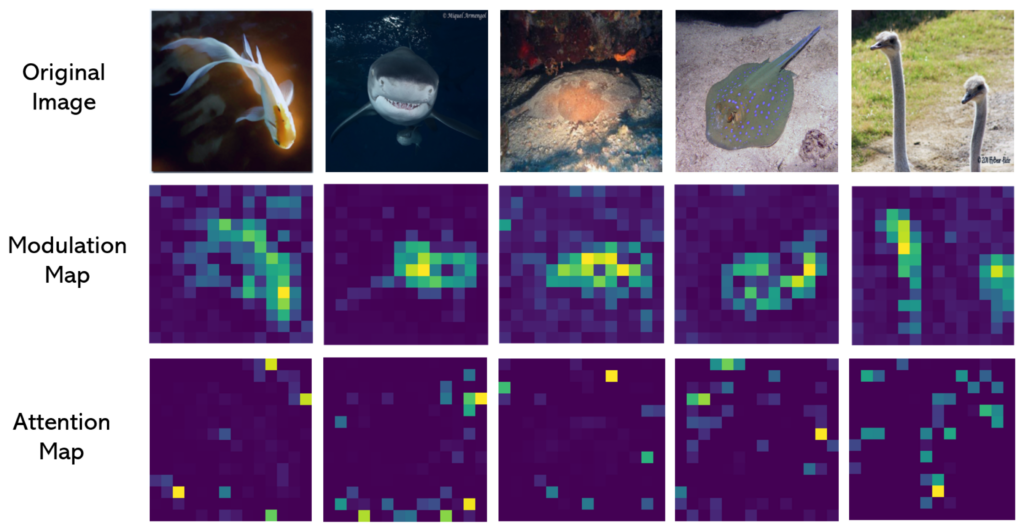
Figure 7: Given an image, we compare the modulation map in our FocalNet-B/16 and the attention map for ViT-B/16. Clearlt, our FocalNet exhibits stronger interpretability than ViT in that it can precisely locate the foreground objects.

	Image Classification						Object Detection					Segmentation
Model	Multi-scale				Monolithic		Mask R-CNN		C. Mask R-CNN			UperNet
	Tiny	Small	Base	Large	Small	Base	Tiny 3$\times$		Tiny 3$\times$			Tiny	Small	Base
Metric	Top-1 Acc.				Top-1 Acc.		APb	APm	APb	AP${}^{b}_{50}$	AP${}^{b}_{75}$	mIoU
ConvNeXt [55]	82.1	83.1	83.8	86.6	79.7	82.0	46.2	41.7	50.4	69.1	54.8	46.7	49.6	49.9
FocalNet (Ours)	82.3	83.5	83.9	86.5	80.9	82.4	47.6	42.6	51.5	70.1	55.8	47.2	50.1	51.1

Table 15: Comparison with ConvNeXts with compiled results on a range of computer vision tasks. The numbers of ConvNeXt are reported in [55].

ViTs [22] is undoubtedly the seminal work that applies Self-Attention for visual modeling. Here, we trace back to the origin and study whether our Focal Modulation can fit the monolithic architectures like ViTs. We replace all SA modules in ViTs with focal modulation to construct monolithic FocalNet-T/S/B. We use patch size 16 and three focal levels with kernel sizes 3,5 and 7, so that the effective receptive field is close to the global SA in ViT.

Model	Dim	#Param.	FLOPs	Th. (imgs/s)	Top-1
ViT-T/16	192	5.7	1.3	2834	72.2
FocalNet-T/16	192	5.9	1.1	2334	74.1 (+1.9)
ViT-S/16	384	22.1	4.6	1060	79.9
FocalNet-S/16	384	22.4	4.3	920	80.9 (+1.0)
ViT-B/16	768	86.6	17.6	330	81.8
FocalNet-B/16	768	87.2	16.9	300	82.4 (+0.6)

Table 16: Comparisons between FocalNet and ViT both with monolithic architectures.

As shown in Table 16, FocalNets consistently outperform ViTs, with similar FLOPs and speed. Besides the quantitative comparisons, we also show the modulation maps and attention maps for FocalNet-B/16 and ViT-B/16 in Fig. 7. FocalNets clearly demonstrate the stronger interpretability than ViTs.

In Sec. 2, we briefly discuss several concurrent works to ours. Among them, ConvNeXts [55] achieved new SoTA on some challenging vision tasks. Here, we quantitatively compare FocalNets with ConvNeXts by summarizing the results on a series of vision tasks in Table 15. FocalNets outperform ConvNeXts in most cases across the board. Our FocalNets use depth-wise convolution as in ConvNeXt for contextualization but also use modulation to inject the contexts to each individual tokens, which makes a significant difference.

5 Conclusion

In this paper, we have proposed Focal Modulation, a new and generic mechanism that enables input-dependent token interactions for visual modeling. It consists of a hierarchical contextualization to gather for each query token its contexts from short- to long-range, a gated aggregation to adaptively aggregate context features based on the query content into modulator, followed by a simple yet effective modulation. With Focal Modulation, we built a series of simple attention-free Focal Modulation Networks (FocalNets) for various vision tasks. Extensive experiments show that FocalNets significantly outperform the SoTA SA counterparts (e.g., Swin and Focal Transformer) with similar time-/memory-cost on the tasks of image classification, object detection and semantic segmentation. Notably, our FocalNets achieved new SoTA performance on COCO object detection with much less parameters and pretraining data than the prior works. These encouraging results render Focal Modulation a favorable and even better choice to SA for effective and efficient visual modeling.

Future works. The main goal of this work is to develop a more effective way for visual token interaction. Though it seems straightforward, a more comprehensive study is needed to verify whether our Focal Modulation can be applied to other domains such as NLP tasks. Moreover, when coping with multi-modal tasks, SA can be feasibly transformed to cross-attention by alternating the queries and keys. The proposed Focal Modulation requires a gather of contexts for individual queries. How to perform the so-called cross-modulation needs more exploration for multi-modal learning.

Acknowledgement.

We would like to thank Lei Zhang, Hao Zhang, Feng Li and Shilong Liu from IDEA team for helpful discussions and detailed instructions of using DINO for object detection. We would like to thank Aishwarya Kamath for sharing the Object365v2 dataset. We would like to thank Lingchen Meng for helping converting contrastive denoising into regular denoising in DINO.

Appendix A More Implementation Details

A.1 Model Configuration

As we discussed in our main submission, we observed in our experiments that different configurations (e.g., depths, dimensions, etc) lead to different performance. For a fair comparison, we use the same stage layouts and hidden dimensions as Swin [54, 95], but replace the SA modules with Focal Modulation modules. We thus construct a series of Focal Modulation Network (FocalNet) variants as shown in Table 17.

Name	Depth	Dimension ($d$)	Levels ($L$)	Kernel Size ($k^{1}$)	Effective Receptive Field ($r^{L}$)
FocalNet-T (SRF/LRF)	[2,2,6,2]	[96,192,384,768]
FocalNet-S (SRF/LRF)	[2,2,18,2]	[96,192,384,768]	[2,2,2,2]	[3,3,3,3]	[7,7,7,7]
FocalNet-B (SRF/LRF)	[2,2,18,2]	[128,256,512,1024]	[3,3,3,3]	[3,3,3,3]	[13,13,13,13]
FocalNet-L (SRF/LRF)	[2,2,18,2]	[192,384,768,1536]
FocalNet-H	[2,2,18,2]	[352,704,1408,2816]	[4,4,4,4]	[3,3,3,3]	[21, 21, 21, 21]

Table 17: Model configurations at four stages for FocalNet. The depth layouts and hidden dimension ($d$) are the same to Swin [54] and Focal Transformers [95]. SRF and LRF means small and large receptive field, respectively. The only difference is the number of focal levels ($L$) and starting kernel size ($k^{\ell=1}$). The last column lists the effective receptive field at top focal level at each stage ($r^{L}$).

A.2 Training settings for ImageNet-1K

We follow Swin [54] to use the same set of data augmentations including Random Augmentation [16], Mixup [107], CutMix [104] and Random Erasing [116]. For model regularization, we use Label Smoothing [68] and DropPath [36]. For all models, the initial learning rate is set to $10^{-3}$ after 20 warm-up epochs beginning with $10^{-6}$. For optimization, we use AdamW [57] and a cosine learning rate scheduler [56]. The weight decay and the gradient clipping norm is set to $0.05$ and $5.0$, respectively. We set the stochastic depth drop rates to $0.2$, $0.3$ and $0.5$ for our tiny, small and base models, respectively. During training, images are randomly cropped to $224\times 224$, and a center crop is used during evaluation. Throughput/Speed is measured on one V100 GPU with batch size 128, following [54]. A detailed summary is shown in Table 18.

Setting	FocalNet-T/S/B (Hierarchical)	FocalNet-T/S/B (Monolithic)
batch size	1024	1024
base learning rate	1e-3	1e-3
learning rate scheduler	cosine	cosine
min learning rate	1e-5	1e-5
training epochs	300	300
warm-up epochs	20	20
warm-up schedule	linear	linear
warm-up learning rate	1e-6	1e-6
optimizer	adamw	adamw
color jitter factor	0.4	0.4
auto-aug	rand-m9-mstd0.5-inc1	rand-m9-mstd0.5-inc1
random-erasing prob.	0.25	0.25
random-erasing mode	pixel	pixel
mixup $\alpha$	0.8	0.8
cutmix $\alpha$	0.8	0.8
mixup prob.	1.0	1.0
mixup switch prob.	0.5	0.5
stochastic drop path rate	0.2/0.3/0.5	0.2/0.2/0.3
label smoothing	0.1	0.1
gradient clip	5.0	5.0
weight decay	0.05	0.05

Table 18: Experimental settings for training on ImageNet-1K with FocalNets.

A.3 Training settings for ImageNet-22K

We train FocalNet-B and FocalNet-L for 90 epochs with a batch size of 4096 and input resolution $224\times 224$. The initial learning rate is set to $10^{-3}$ after a warmup of 5 epochs. We set the the stochastic depth drop rates to $0.2$ for both networks. For stability, we use LayerScale [77] with initial value $10^{-4}$ for all layers. The other settings follow those for ImageNet-1K. After the pretraining, we finetune the models on ImageNet-1K for 30 epochs with initial learning rate of $3\times 10^{-5}$, cosine learning rate scheduler and AdamW optimizer. The stochastic depth drop rate is set to $0.3$ and both CutMix and Mixup are muted during the finetuning.

A.4 Training settings for Object365

We exactly follow the settings in DINO [106] to pretrain our object detection models on Object365 [62]. In total, Object365 contains around 1.7M images for training and 80k for validation. We merge 75k validation images to the training data and use the remained for evaluation during the pretraining. We pre-train FocalNets+DINO for 26 epochs with learning rate $1e^{-4}$, and drop the learning rate by 10 times after 24 epochs. A standard image resolution $800\times 1333$ is used. After the pretraining, we finetune the model on COCO with max size $1200\times 2000$. We lower the learning rate to $6e^{-5}$ and train the model for 12 epochs in total.

Setting	FocalNet-B/L (Pretraining)	FocalNet-B/L (Finetuning)
resolution	224$\times$224	224$\times$224 and 384$\times$384
batch size	4096	1024
base learning rate	1e-3	3e-5
learning rate scheduler	cosine	cosine
min learning rate	1e-5	5e-6
training epochs	90	30
warm-up epochs	5	0
warm-up schedule	linear	linear
warm-up learning rate	1e-6	1e-6
optimizer	adamw	adamw
color jitter factor	0.4	0.4
auto-aug	rand-m9-mstd0.5-inc1	rand-m9-mstd0.5-inc1
random-erasing prob.	0.25	0.25
random-erasing mode	pixel	pixel
mixup $\alpha$	0.8	n/a
cutmix $\alpha$	0.8	n/a
mixup prob.	1.0	n/a
mixup switch prob.	0.5	n/a
initial layer scale	1e-4	pretrained
stochastic drop path rate	0.2/0.2	0.3
label smoothing	0.1	0.1
gradient clip	5.0	5.0
weight decay	0.05	1e-8

Table 19: Experimental settings for pretraining on ImageNet-22K with FocalNet-B/L and finetuning on ImageNet-1K.

Appendix B Downstream Tasks

B.1 Object Detection

B.1.1 Effect of kernel size

We study how the various kernel sizes affect the object detection performance when finetuning FocalNet-T (LRF) with $k^{\ell=1}=3$ pretrained on ImageNet-1K. In Fig. 9, we vary the kernel size at first level $k^{\ell=1}$ from 3 to 15 for object detection finetuning. We have two interesting observations: $(i)$ though the pretrained model used $k^{\ell=1}=3$, it can be finetuned with different kernel sizes to adapt high-resolution object detection task; $(ii)$ a moderate kernel size (5,7,9,11) have a slightly better performance than a kernel size which is too small (3) or too big (13,15), probably because small kernel cannot capture the long-range dependency while big kernel misses the detailed local context. In Fig. 9, we further show the corresponding wall-clock time cost and peak memory when training on 16 V100 GPUs with batch size 16. Accordingly, increasing the kernel size gradually increases the training memory and time cost. For a good performance/cost trade-off, we therefore set $k^{\ell=1}=9$ for all the object detection finetuning experiments in our main submission.

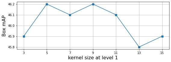
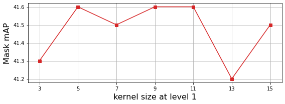
Figure 8: Box and mask mAP for Mask R-CNN 1$\times$ training. We use FocalNet-T (LRF) as the baseline model and vary its kernel size at first level $k^{\ell=1}\in\{3,5,7,9,11,13,15\}$.

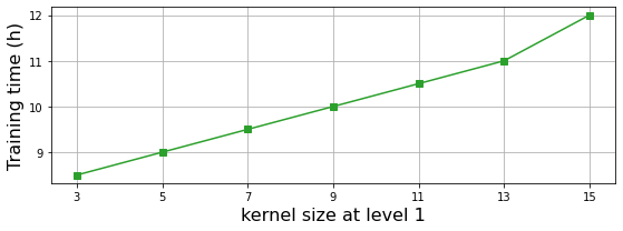
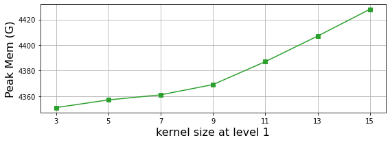
Figure 9: Training time (wall-clock) and peak memory for Mask R-CNN 1$\times$. We train Focalnet-T (LRF) with different kernel sizes on 16 V100 GPUs with batch size 16.

Backbone	#Params	FLOPs	Mask R-CNN 1x						Mask R-CNN 3x
	(M)	(G)	$AP^{b}$	$AP^{b}_{50}$	$AP^{b}_{75}$	$AP^{m}$	$AP^{m}_{50}$	$AP^{m}_{75}$	$AP^{b}$	$AP^{b}_{50}$	$AP^{b}_{75}$	$AP^{m}$	$AP^{m}_{50}$	$AP^{m}_{75}$
FocalNet-T (SRF)	48.6	267	45.9	68.3	50.1	41.3	65.0	44.3	47.6	69.5	52.0	42.6	66.5	45.6
FocalNet-T (LRF)	48.9	268	46.1	68.2	50.6	41.5	65.1	44.5	48.0	69.7	53.0	42.9	66.5	46.1
FocalNet-T (SRF)$\dagger$	45.8	261	46.8	69.1	51.2	41.9	65.6	44.6	48.5	70.0	53.2	43.3	67.0	46.3
FocalNet-S (SRF)	70.8	356	48.0	69.9	52.7	42.7	66.7	45.7	48.9	70.1	53.7	43.6	67.1	47.1
FocalNet-S (LRF)	72.3	365	48.3	70.5	53.1	43.1	67.4	46.2	49.3	70.7	54.2	43.8	67.9	47.4
FocalNet-S (SRF)$\dagger$	59.5	312	48.1	70.5	52.8	43.1	67.2	46.2	49.2	70.6	53.9	43.8	67.6	47.2
FocalNet-B (SRF)	109.4	496	48.8	70.7	53.5	43.3	67.5	46.5	49.6	70.6	54.1	44.1	68.0	47.2
FocalNet-B (LRF)	111.4	507	49.0	70.9	53.9	43.5	67.9	46.7	49.8	70.9	54.6	44.1	68.2	47.2
FocalNet-B (SRF)$\dagger$	107.1	481	49.6	71.2	54.6	44.0	68.2	47.6	50.2	71.0	55.0	44.3	68.1	47.9

Table 20: Gray rows are additional results using deeper but thinner FocalNets in Table 4 as the backbone.

B.1.2 Results with deeper and thinner FocalNets

In our main submission, we compared with previous SoTA methods Swin and Focal Transformer in a restricted way by using the same network depth layout. Meanwhile, we also showed that different depth layouts lead to different image classification performance. Here, we investigate how the layout affects the object detection performance. We use the deeper but thinner FocalNets in Table 4 of our main submission as the backbones. Specifically, we change the depth layout of our FocalNet-T from 2-2-6-2 to 3-3-16-3, and FocalNet-S/B from 2-2-18-2 to 4-4-28-4. Meanwhile, we reduce the initial hidden dimension from 96, 128 to 64, 96, respectively. In Table 20, we add the additional gray rows to compare with the results reported in our main submission. In Table 22, we further show the 1$\times$ results of deeper and thinner FocalNets with large receptive field. Accordingly, the object detection performance (both box and mask mAP) are boosted over the shallower and wider version of FocalNets with same receptive field. On one hand, this trend suggests a feasible way to improve the performance for our FocalNet, and further demonstrate its effectiveness for both image classification and object detection. On the other hand, it suggests that keeping network configuration (depth, hidden dimension, etc.) the same is important for a fair comparison with previous works.

B.2 Image Segmentation

In Table 22, we report the results using the deeper and thinner FocalNets as the backbone for semantic segmentation. As we can see, for FocalNet-T, increasing the depth does not bring extra improvement. For larger models, however, a deeper version outperforms the shallow ones, particularly on FocalNet-B. Additionally, we further compare with most recent work MPViT [39] which also exploits multi-scale features but in parallel manner. As we can see, our FocalNets achieve better performance than MPViT with comparable cost. Compared with MPViT, the hierarchical and gated contextualization proposed in FocalNets can rapidly cover large receptive field facilitating the high-resolution dense prediction tasks.

Backbone	#Param.	FLOPs	APb	APm
Swin-Tiny	47.8	264	43.7	39.8
FocalAtt-Tiny	48.8	291	44.8	41.0
FocalNet-T (SRF)	48.6	267	45.9	41.3
FocalNet-T (SRF)$\dagger$	45.8	261	46.8	41.9
FocalNet-T (LRF)	48.9	268	46.1	41.5
FocalNet-T (LRF)$\dagger$	46.1	262	46.7	41.9
Swin-Small	69.1	354	46.5	42.1
FocalAtt-Small	71.2	401	47.4	42.8
FocalNet-S (SRF)	70.8	356	48.0	42.7
FocalNet-S (SRF)$\dagger$	59.5	312	48.1	43.1
FocalNet-S (LRF)	72.3	365	48.3	43.1
FocalNet-S (LRF)$\dagger$	60.0	315	48.6	43.3
Swin-Base	107.1	497	46.9	42.3
FocalAtt-Base	110.0	533	47.8	43.3
FocalNet-B (SRF)	109.4	496	48.8	43.3
FocalNet-B (SRF)$\dagger$	107.1	481	49.6	44.0
FocalNet-B (LRF)	111.4	507	49.0	43.5
FocalNet-B (LRF)$\dagger$	107.9	485	49.9	44.2

Table 21: Additional results of Mask R-CNN 1$\times$ with deeper and thinner FocalNets (LRF) in gray rows. We use the same pretrained model as FocalNet (SRF)$\dagger$, but add an extra focal level on top with kernel initialized with all-zeros.

Backbone	#Param.	FLOPs	mIoU	+MS
Swin-T [54]	60	941	44.5	45.8
FocalAtt-T [95]	62	998	45.8	47.0
FocalNet-T (SRF)	61	944	46.5	47.2
FocalNet-T (LRF)	61	949	46.8	47.8
FocalNet-T (SRF)$\dagger$	55	934	47.4	48.5
Swin-S [54]	81	1038	47.6	49.5
FocalAtt-S [95]	85	1130	48.0	50.0
MPViT-S [39]	52	943	48.3	n/a
FocalNet-S (SRF)	83	1035	49.3	50.1
FocalNet-S (LRF)	84	1044	49.1	50.1
FocalNet-S (SRF)$\dagger$	69	986	49.4	50.3
Swin-B [54]	121	1188	48.1	49.7
FocalAtt-B [95]	126	1354	49.0	50.5
MPViT-B [39]	105	1186	50.3	n/a
FocalNet-B (SRF)	124	1180	50.2	51.1
FocalNet-B (LRF)	126	1192	50.5	51.4
FocalNet-B (SRF)$\dagger$	117	1159	51.0	51.9

Table 22: Semantic segmentation on ADE20K [118]. All models are trained with UperNet [90]. Grays rows are additional results with deeper yet thinner FocalNets (SRF).

Appendix C Additional Model Interpretation

Our focal modulation consists of three main components: $(i)$ convolution for contextualization; $(ii)$ gating mechanism for aggregation of multiple granularity and $(iii)$ linear projection for generating modulator. Here we attempt to interpret each of them.

Convolutional kernel patterns at different levels and layers.

In Fig. 11 and Fig. 11, we show the learned depth-wise convolutional kernels in our FocalNet-T (LRF) and FocalNet-B (LRF). Specifically, we show the averaged 3$\times$3, 5$\times$5 and 7$\times$7 kernels at last layer of each of four stages. We observe some interesting patterns from the visualizations. In the earlier stage, the models usually focus on local regions and thus have more scattered weights at low focal levels (level 1 and 2). Nevertheless, when it comes to later stage, the model requires more global context to make the final prediction, which explains the more scattered weights at the third focal level.

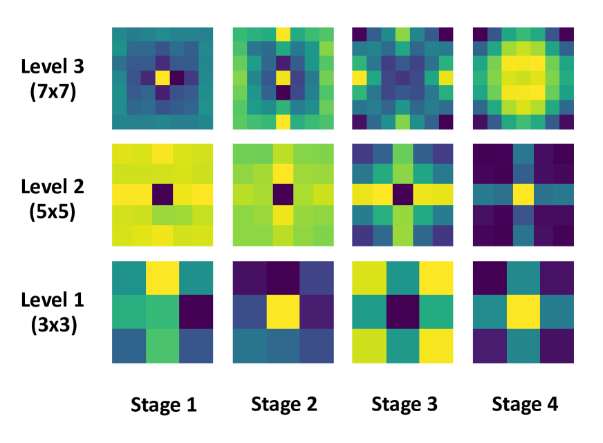
Figure 10: Visualization of learned kernels at three levels and four stages in FocalNet-T (LRF). For clarity, we only show for the last layer of each stage.

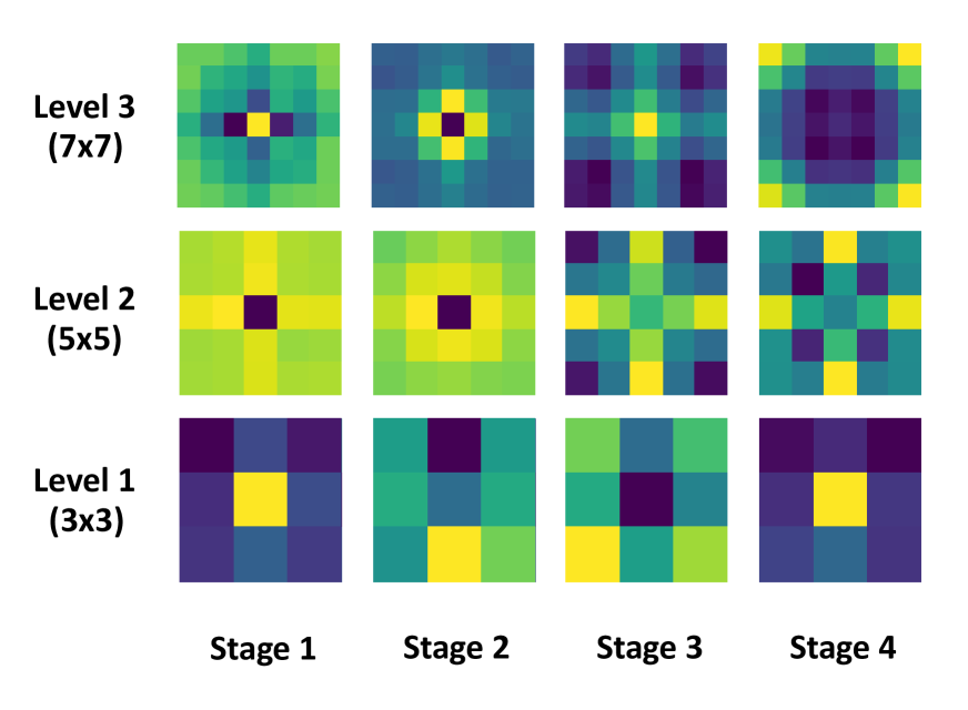
Figure 11: Visualization of learned kernels at three levels and four stages in FocalNet-B (LRF). For clarity, we only show for the last layer at each stage.

Gating function for adaptive contextualization.

Similar to Fig. 6, we make more visualizations of the gating values in our FocalNets. On a set of randomly selected ImageNet-1K validation images, we show more gating maps in Fig. 12, 13 and 14. For the visual tokens at object regions ($\ell=1$), their gating values are much higher than those outside object regions at first level. When looking more closely, we can see that the predicted gating values mainly lie on the most complicated textures within object regions. At the second level $\ell=2$, the gating values are still higher in object regions but the peak values usually move to the object boundaries instead. At the third level $\ell=3$, the whole object regions have higher gating values than background regions. Finally at level $\ell=4$, we find there is a clear distinction between foreground and background regions when aggregating the global contexts. The foreground regions usually show less interest in the global context and the other way around for the background regions. Even for those images containing multiple foreground objects, our model still shows coherent patterns. Comparing the gating values for first three levels and the last global context, we can find our model does gather more information from local regions when modulating foreground visual tokens and more global context for background tokens.

Modulator is a new way of attention.

As we showed earlier, the modulator ${\bf M}$ computed at the last layer of our FocalNet shows an emerge of object localization capacity even though no class guidance is provided, unlike CAM [117] or Grad-CAM [61]. We show additional visualizations in Fig. 15. They clearly show that our FocalNets is good at localizing the most discriminative regions from the image and thus spending more effort to modulate these regions to produce the final predictions. We strongly believe this property emerged in our proposed Focal Modulation mechanism opens up a new door for the community on how to interpret the models beyond the gradient-based and class-guided methods. We will leave studies on the correlations between the modulators and the correctness of final predictions, and the robustness of our FocalNets as future works. We refer the readers to try our online modulator visualization demo at https://huggingface.co/spaces/jw2yang/focalnet-modulators.

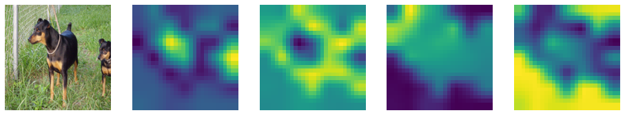
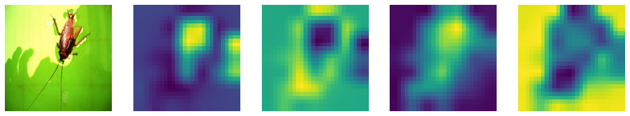
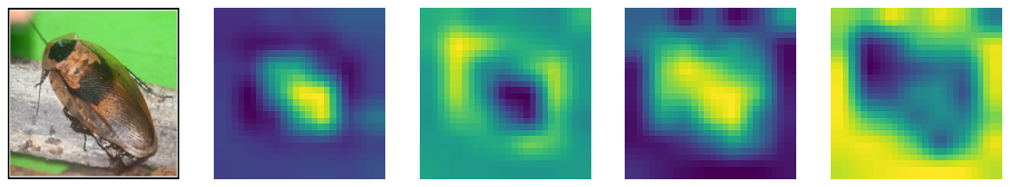
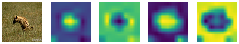
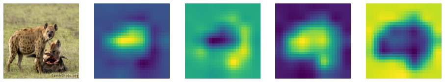
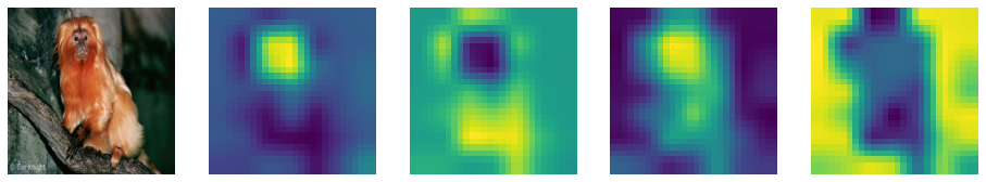
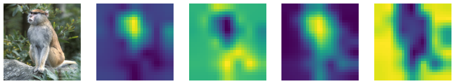
Figure 12: Visualization of gating values ${\bf G}$ at last layer of our FocalNet-B (LRF) pretrained on ImageNet-1K. From left to right, we show input image, and gating weights ${\bf G}^{\ell},\ell=1,2,3,4$.

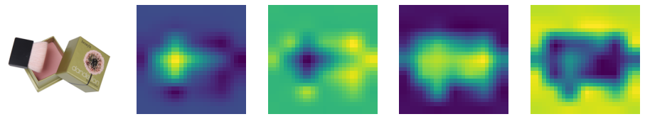
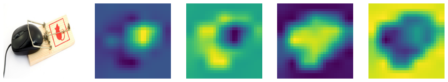
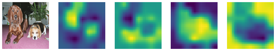
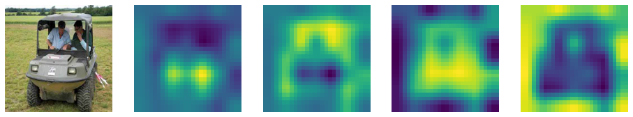
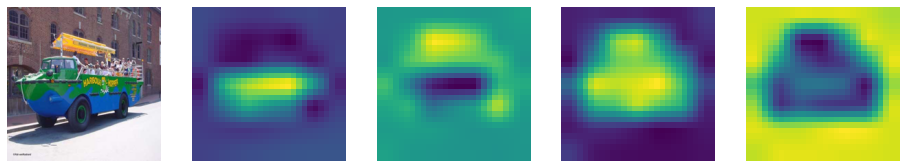
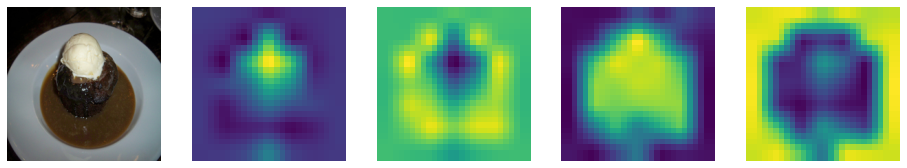
Figure 13: Visualization of gating values ${\bf G}$ at last layer of our FocalNet-B (LRF) pretrained on ImageNet-1K. The order from left to right column is same to Fig. 12

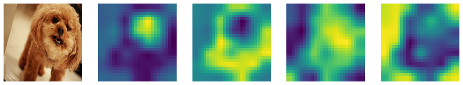
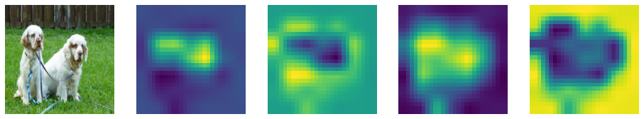
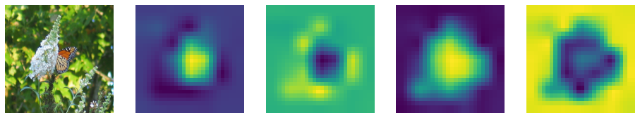
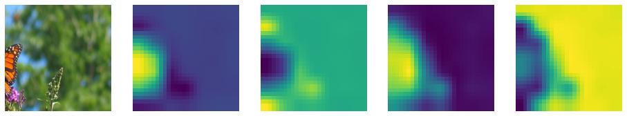
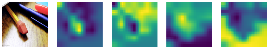
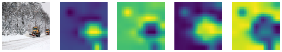
Figure 14: Visualization of gating values ${{\bf G}}$ at last layer of our FocalNet-B (LRF) pretrained on ImageNet-1K. The order from left to right column is same to Fig. 12

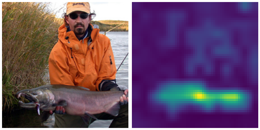
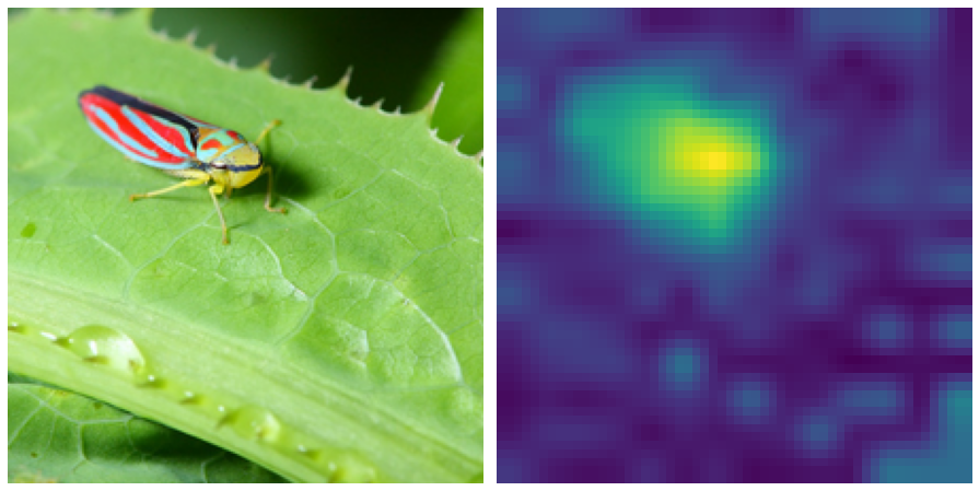
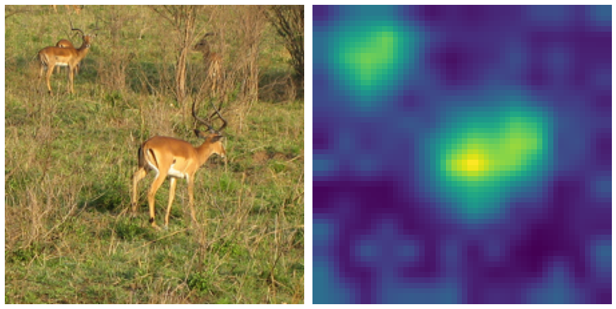
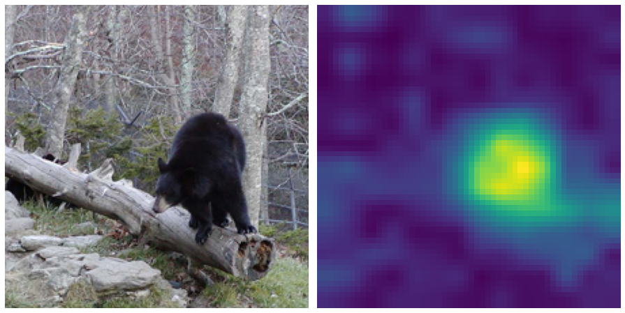
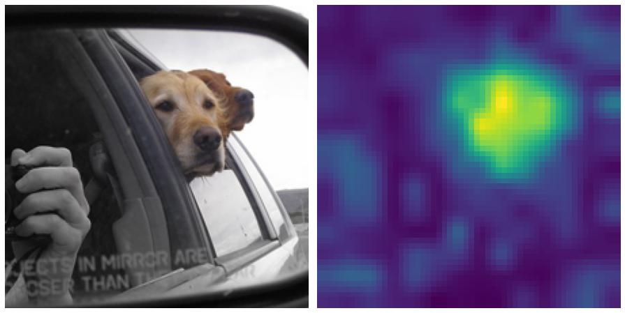
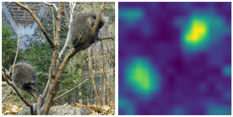
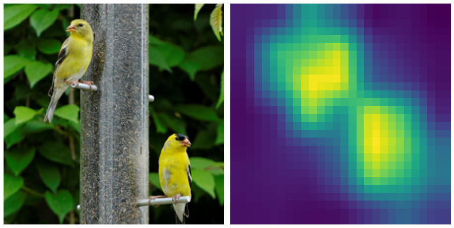
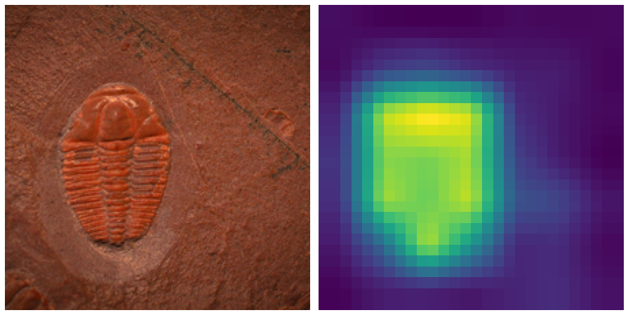
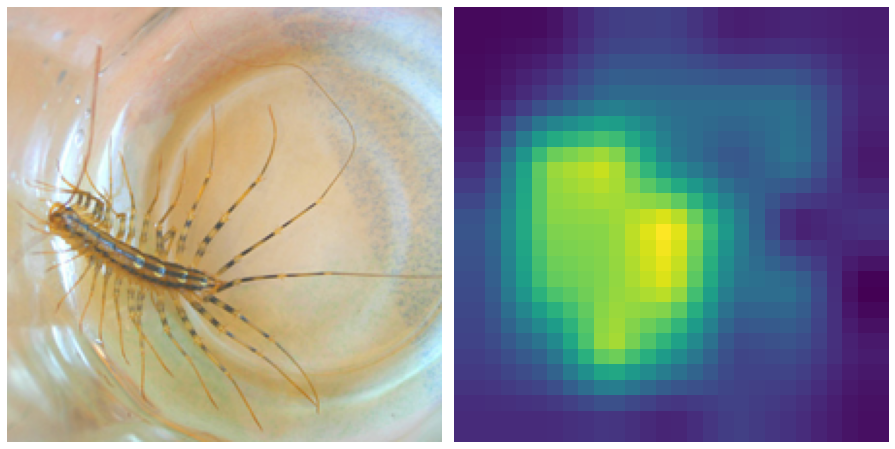
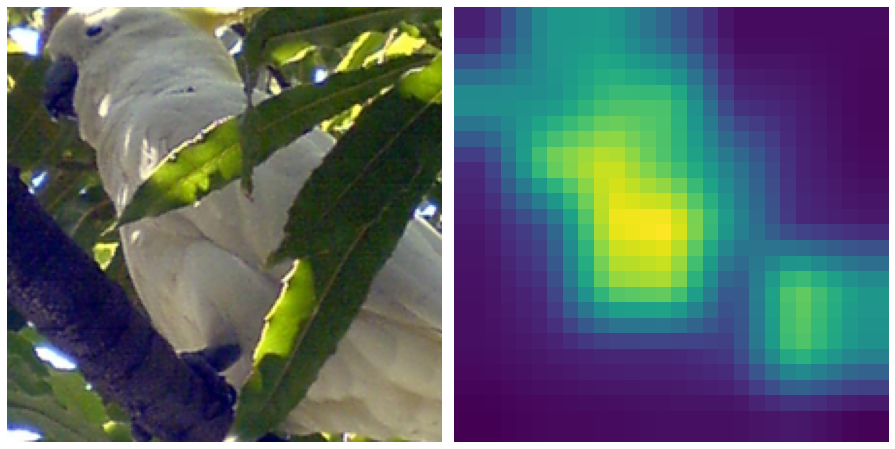
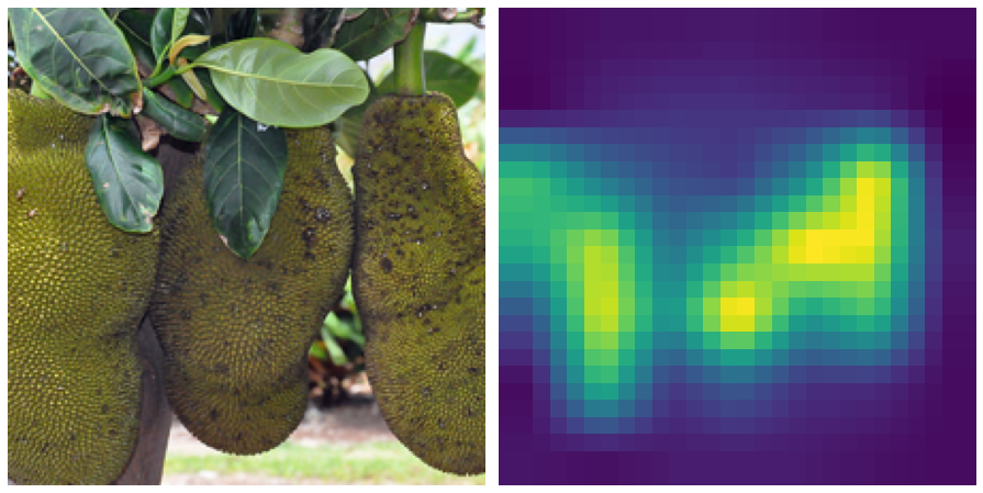
Figure 15: Visualization of modulator at the top layer of FocalNets. We show the magnitude ($L$-2 norm) of the modulator vector pixel-wise for each input image. The heatmaps clearly show the “attention” of our FocalNets for free. The top three rows are with the monolithical FocalNet-B/16 and the bottom three rows are for the hierarchical FocalNet-Base.

Appendix D Social Impact

This work is mainly focused on architecture design for computer vision tasks. We have trained the models on various datasets and tasks. One concern is that it might be biased to the training data. When it is trained on large-scale webly-crawled image data, the negative impact might be amplified due to the potential offensive or biased contents in the data. To avoid this, we need to have a careful sanity check on the training data and the model’s predictions before training the model and deploying it to the realistic applications.

References

- [1] Zhaowei Cai and Nuno Vasconcelos. Cascade r-cnn: Delving into high quality object detection. In Proceedings of the IEEE conference on computer vision and pattern recognition, pages 6154–6162, 2018.
- [2] Yue Cao, Jiarui Xu, Stephen Lin, Fangyun Wei, and Han Hu. Gcnet: Non-local networks meet squeeze-excitation networks and beyond. In Proceedings of the IEEE/CVF International Conference on Computer Vision Workshops, pages 0–0, 2019.
- [3] Nicolas Carion, Francisco Massa, Gabriel Synnaeve, Nicolas Usunier, Alexander Kirillov, and Sergey Zagoruyko. End-to-end object detection with transformers. In European Conference on Computer Vision, pages 213–229. Springer, 2020.
- [4] Shuning Chang, Pichao Wang, Fan Wang, Hao Li, and Jiashi Feng. Augmented transformer with adaptive graph for temporal action proposal generation. arXiv preprint arXiv:2103.16024, 2021.
- [5] Chun-Fu Chen, Quanfu Fan, and Rameswar Panda. Crossvit: Cross-attention multi-scale vision transformer for image classification, 2021.
- [6] Liang-Chieh Chen, Yukun Zhu, George Papandreou, Florian Schroff, and Hartwig Adam. Encoder-decoder with atrous separable convolution for semantic image segmentation. In Proceedings of the European conference on computer vision (ECCV), pages 801–818, 2018.
- [7] Qiang Chen, Qiman Wu, Jian Wang, Qinghao Hu, Tao Hu, Errui Ding, Jian Cheng, and Jingdong Wang. Mixformer: Mixing features across windows and dimensions. In Proceedings of the IEEE/CVF Conference on Computer Vision and Pattern Recognition, pages 5249–5259, 2022.
- [8] Shoufa Chen, Enze Xie, Chongjian Ge, Ding Liang, and Ping Luo. CycleMLP: A mlp-like architecture for dense prediction. arXiv preprint arXiv:2107.10224, 2021.
- [9] Xin Chen, Bin Yan, Jiawen Zhu, Dong Wang, Xiaoyun Yang, and Huchuan Lu. Transformer tracking. arXiv preprint arXiv:2103.15436, 2021.
- [10] Yinpeng Chen, Xiyang Dai, Mengchen Liu, Dongdong Chen, Lu Yuan, and Zicheng Liu. Dynamic convolution: Attention over convolution kernels. In Proceedings of the IEEE/CVF Conference on Computer Vision and Pattern Recognition, pages 11030–11039, 2020.
- [11] Zhe Chen, Yuchen Duan, Wenhai Wang, Junjun He, Tong Lu, Jifeng Dai, and Yu Qiao. Vision transformer adapter for dense predictions. arXiv preprint arXiv:2205.08534, 2022.
- [12] Bowen Cheng, Ishan Misra, Alexander G Schwing, Alexander Kirillov, and Rohit Girdhar. Masked-attention mask transformer for universal image segmentation. arXiv preprint arXiv:2112.01527, 2021.
- [13] Bowen Cheng, Ishan Misra, Alexander G Schwing, Alexander Kirillov, and Rohit Girdhar. Masked-attention mask transformer for universal image segmentation. In Proceedings of the IEEE/CVF Conference on Computer Vision and Pattern Recognition, pages 1290–1299, 2022.
- [14] Bowen Cheng, Alex Schwing, and Alexander Kirillov. Per-pixel classification is not all you need for semantic segmentation. Advances in Neural Information Processing Systems, 34, 2021.
- [15] Xiangxiang Chu, Zhi Tian, Yuqing Wang, Bo Zhang, Haibing Ren, Xiaolin Wei, Huaxia Xia, and Chunhua Shen. Twins: Revisiting spatial attention design in vision transformers. arXiv preprint arXiv:2104.13840, 2021.
- [16] Ekin D Cubuk, Barret Zoph, Jonathon Shlens, and Quoc V Le. Randaugment: Practical automated data augmentation with a reduced search space. In Proceedings of the IEEE/CVF Conference on Computer Vision and Pattern Recognition Workshops, pages 702–703, 2020.
- [17] Xiyang Dai, Yinpeng Chen, Bin Xiao, Dongdong Chen, Mengchen Liu, Lu Yuan, and Lei Zhang. Dynamic head: Unifying object detection heads with attentions. In Proceedings of the IEEE/CVF Conference on Computer Vision and Pattern Recognition, pages 7373–7382, 2021.
- [18] Zhigang Dai, Bolun Cai, Yugeng Lin, and Junying Chen. Up-detr: Unsupervised pre-training for object detection with transformers. arXiv preprint arXiv:2011.09094, 2020.
- [19] Jia Deng, Wei Dong, Richard Socher, Li-Jia Li, Kai Li, and Li Fei-Fei. Imagenet: A large-scale hierarchical image database. In 2009 IEEE conference on computer vision and pattern recognition, pages 248–255. Ieee, 2009.
- [20] Mingyu Ding, Bin Xiao, Noel Codella, Ping Luo, Jingdong Wang, and Lu Yuan. Davit: Dual attention vision transformers. arXiv preprint arXiv:2204.03645, 2022.
- [21] Xiaoyi Dong, Jianmin Bao, Dongdong Chen, Weiming Zhang, Nenghai Yu, Lu Yuan, Dong Chen, and Baining Guo. Cswin transformer: A general vision transformer backbone with cross-shaped windows. arXiv preprint arXiv:2107.00652, 2021.
- [22] Alexey Dosovitskiy, Lucas Beyer, Alexander Kolesnikov, Dirk Weissenborn, Xiaohua Zhai, Thomas Unterthiner, Mostafa Dehghani, Matthias Minderer, Georg Heigold, Sylvain Gelly, et al. An image is worth 16x16 words: Transformers for image recognition at scale. arXiv preprint arXiv:2010.11929, 2020.
- [23] Peng Gao, Jiasen Lu, Hongsheng Li, Roozbeh Mottaghi, and Aniruddha Kembhavi. Container: Context aggregation network. arXiv preprint arXiv:2106.01401, 2021.
- [24] Chengyue Gong, Dilin Wang, Meng Li, Vikas Chandra, and Qiang Liu. Vision transformers with patch diversification, 2021.
- [25] Jianyuan Guo, Kai Han, Han Wu, Chang Xu, Yehui Tang, Chunjing Xu, and Yunhe Wang. Cmt: Convolutional neural networks meet vision transformers. arXiv preprint arXiv:2107.06263, 2021.
- [26] Jianyuan Guo, Yehui Tang, Kai Han, Xinghao Chen, Han Wu, Chao Xu, Chang Xu, and Yunhe Wang. Hire-mlp: Vision mlp via hierarchical rearrangement. arXiv preprint arXiv:2108.13341, 2021.
- [27] Kai Han, Yunhe Wang, Hanting Chen, Xinghao Chen, Jianyuan Guo, Zhenhua Liu, Yehui Tang, An Xiao, Chunjing Xu, Yixing Xu, et al. A survey on visual transformer. arXiv preprint arXiv:2012.12556, 2020.
- [28] Qi Han, Zejia Fan, Qi Dai, Lei Sun, Ming-Ming Cheng, Jiaying Liu, and Jingdong Wang. Demystifying local vision transformer: Sparse connectivity, weight sharing, and dynamic weight. arXiv preprint arXiv:2106.04263, 2021.
- [29] Kaiming He, Georgia Gkioxari, Piotr Dollár, and Ross Girshick. Mask r-cnn. In Proceedings of the IEEE international conference on computer vision, pages 2961–2969, 2017.
- [30] Kaiming He, Xiangyu Zhang, Shaoqing Ren, and Jian Sun. Deep residual learning for image recognition. In Proceedings of the IEEE conference on computer vision and pattern recognition, pages 770–778, 2016.
- [31] Dan Hendrycks and Kevin Gimpel. Gaussian error linear units (gelus). arXiv preprint arXiv:1606.08415, 2016.
- [32] Qibin Hou, Zihang Jiang, Li Yuan, Ming-Ming Cheng, Shuicheng Yan, and Jiashi Feng. Vision permutator: A permutable mlp-like architecture for visual recognition. arXiv preprint arXiv:2106.12368, 2021.
- [33] Andrew G Howard, Menglong Zhu, Bo Chen, Dmitry Kalenichenko, Weijun Wang, Tobias Weyand, Marco Andreetto, and Hartwig Adam. Mobilenets: Efficient convolutional neural networks for mobile vision applications. arXiv preprint arXiv:1704.04861, 2017.
- [34] Han Hu, Zheng Zhang, Zhenda Xie, and Stephen Lin. Local relation networks for image recognition. In Proceedings of the IEEE/CVF International Conference on Computer Vision, pages 3464–3473, 2019.
- [35] Jie Hu, Li Shen, and Gang Sun. Squeeze-and-excitation networks. In Proceedings of the IEEE conference on computer vision and pattern recognition, pages 7132–7141, 2018.
- [36] Gao Huang, Yu Sun, Zhuang Liu, Daniel Sedra, and Kilian Q Weinberger. Deep networks with stochastic depth. In European conference on computer vision, pages 646–661. Springer, 2016.
- [37] Jitesh Jain, Anukriti Singh, Nikita Orlov, Zilong Huang, Jiachen Li, Steven Walton, and Humphrey Shi. Semask: Semantically masked transformers for semantic segmentation. arXiv preprint arXiv:2112.12782, 2021.
- [38] Salman Khan, Muzammal Naseer, Munawar Hayat, Syed Waqas Zamir, Fahad Shahbaz Khan, and Mubarak Shah. Transformers in vision: A survey. arXiv preprint arXiv:2101.01169, 2021.
- [39] Youngwan Lee, Jonghee Kim, Jeff Willette, and Sung Ju Hwang. Mpvit: Multi-path vision transformer for dense prediction. arXiv preprint arXiv:2112.11010, 2021.
- [40] Youngwan Lee, Jonghee Kim, Jeffrey Willette, and Sung Ju Hwang. Mpvit: Multi-path vision transformer for dense prediction. In Proceedings of the IEEE/CVF Conference on Computer Vision and Pattern Recognition, pages 7287–7296, 2022.
- [41] Bing Li, Cheng Zheng, Silvio Giancola, and Bernard Ghanem. Sctn: Sparse convolution-transformer network for scene flow estimation. arXiv preprint arXiv:2105.04447, 2021.
- [42] Chunyuan Li, Haotian Liu, Liunian Harold Li, Pengchuan Zhang, Jyoti Aneja, Jianwei Yang, Ping Jin, Houdong Hu, Zicheng Liu, Yong Jae Lee, and Jianfeng Gao. ELEVATER: A benchmark and toolkit for evaluating language-augmented visual models. In NeurIPS Track on Datasets and Benchmarks, 2022.
- [43] Duo Li, Jie Hu, Changhu Wang, Xiangtai Li, Qi She, Lei Zhu, Tong Zhang, and Qifeng Chen. Involution: Inverting the inherence of convolution for visual recognition. In Proceedings of the IEEE/CVF Conference on Computer Vision and Pattern Recognition, pages 12321–12330, 2021.
- [44] Liunian Harold Li, Pengchuan Zhang, Haotian Zhang, Jianwei Yang, Chunyuan Li, Yiwu Zhong, Lijuan Wang, Lu Yuan, Lei Zhang, Jenq-Neng Hwang, et al. Grounded language-image pre-training. In Proceedings of the IEEE/CVF Conference on Computer Vision and Pattern Recognition, pages 10965–10975, 2022.
- [45] Xiangyu Li, Yonghong Hou, Pichao Wang, Zhimin Gao, Mingliang Xu, and Wanqing Li. Trear: Transformer-based rgb-d egocentric action recognition. arXiv preprint arXiv:2101.03904, 2021.
- [46] Yawei Li, Kai Zhang, Jiezhang Cao, Radu Timofte, and Luc Van Gool. Localvit: Bringing locality to vision transformers. arXiv preprint arXiv:2104.05707, 2021.
- [47] Zhiqi Li, Wenhai Wang, Enze Xie, Zhiding Yu, Anima Anandkumar, Jose M. Alvarez, Tong Lu, and Ping Luo. Panoptic segformer: Delving deeper into panoptic segmentation with transformers, 2021.
- [48] Dongze Lian, Zehao Yu, Xing Sun, and Shenghua Gao. As-mlp: An axial shifted mlp architecture for vision. arXiv preprint arXiv:2107.08391, 2021.
- [49] Tsung-Yi Lin, Michael Maire, Serge Belongie, James Hays, Pietro Perona, Deva Ramanan, Piotr Dollár, and C Lawrence Zitnick. Microsoft COCO: Common objects in context. In ECCV, 2014.
- [50] Hanxiao Liu, Zihang Dai, David So, and Quoc Le. Pay attention to mlps. Advances in Neural Information Processing Systems, 34, 2021.
- [51] Hanxiao Liu, Zihang Dai, David R So, and Quoc V Le. Pay attention to MLPs. arXiv preprint arXiv:2105.08050, 2021.
- [52] Ze Liu, Han Hu, Yutong Lin, Zhuliang Yao, Zhenda Xie, Yixuan Wei, Jia Ning, Yue Cao, Zheng Zhang, Li Dong, et al. Swin transformer v2: Scaling up capacity and resolution. arXiv preprint arXiv:2111.09883, 2021.
- [53] Ze Liu, Han Hu, Yutong Lin, Zhuliang Yao, Zhenda Xie, Yixuan Wei, Jia Ning, Yue Cao, Zheng Zhang, Li Dong, et al. Swin transformer v2: Scaling up capacity and resolution. In Proceedings of the IEEE/CVF Conference on Computer Vision and Pattern Recognition, pages 12009–12019, 2022.
- [54] Ze Liu, Yutong Lin, Yue Cao, Han Hu, Yixuan Wei, Zheng Zhang, Stephen Lin, and Baining Guo. Swin transformer: Hierarchical vision transformer using shifted windows. arXiv preprint arXiv:2103.14030, 2021.
- [55] Zhuang Liu, Hanzi Mao, Chao-Yuan Wu, Christoph Feichtenhofer, Trevor Darrell, and Saining Xie. A convnet for the 2020s. arXiv preprint arXiv:2201.03545, 2022.
- [56] Ilya Loshchilov and Frank Hutter. Sgdr: Stochastic gradient descent with warm restarts. arXiv preprint arXiv:1608.03983, 2016.
- [57] Ilya Loshchilov and Frank Hutter. Decoupled weight decay regularization. arXiv preprint arXiv:1711.05101, 2017.
- [58] Yuxuan Lou, Fuzhao Xue, Zangwei Zheng, and Yang You. Sparse-mlp: A fully-mlp architecture with conditional computation. arXiv preprint arXiv:2109.02008, 2021.
- [59] Lingchen Meng, Hengduo Li, Bor-Chun Chen, Shiyi Lan, Zuxuan Wu, Yu-Gang Jiang, and Ser-Nam Lim. Adavit: Adaptive vision transformers for efficient image recognition. In Proceedings of the IEEE/CVF Conference on Computer Vision and Pattern Recognition, pages 12309–12318, 2022.
- [60] Yongming Rao, Wenliang Zhao, Benlin Liu, Jiwen Lu, Jie Zhou, and Cho-Jui Hsieh. Dynamicvit: Efficient vision transformers with dynamic token sparsification. Advances in neural information processing systems, 34:13937–13949, 2021.
- [61] Ramprasaath R Selvaraju, Michael Cogswell, Abhishek Das, Ramakrishna Vedantam, Devi Parikh, and Dhruv Batra. Grad-cam: Visual explanations from deep networks via gradient-based localization. In Proceedings of the IEEE international conference on computer vision, pages 618–626, 2017.
- [62] Shuai Shao, Zeming Li, Tianyuan Zhang, Chao Peng, Gang Yu, Xiangyu Zhang, Jing Li, and Jian Sun. Objects365: A large-scale, high-quality dataset for object detection. In Proceedings of the IEEE international conference on computer vision, pages 8430–8439, 2019.
- [63] Karen Simonyan and Andrew Zisserman. Very deep convolutional networks for large-scale image recognition. arXiv preprint arXiv:1409.1556, 2014.
- [64] Robin Strudel, Ricardo Garcia, Ivan Laptev, and Cordelia Schmid. Segmenter: Transformer for semantic segmentation. arXiv preprint arXiv:2105.05633, 2021.
- [65] Ke Sun, Bin Xiao, Dong Liu, and Jingdong Wang. Deep high-resolution representation learning for human pose estimation. In CVPR, 2019.
- [66] Peize Sun, Rufeng Zhang, Yi Jiang, Tao Kong, Chenfeng Xu, Wei Zhan, Masayoshi Tomizuka, Lei Li, Zehuan Yuan, Changhu Wang, et al. Sparse r-cnn: End-to-end object detection with learnable proposals. arXiv preprint arXiv:2011.12450, 2020.
- [67] Christian Szegedy, Wei Liu, Yangqing Jia, Pierre Sermanet, Scott Reed, Dragomir Anguelov, Dumitru Erhan, Vincent Vanhoucke, and Andrew Rabinovich. Going deeper with convolutions. In Proceedings of the IEEE conference on computer vision and pattern recognition, pages 1–9, 2015.
- [68] Christian Szegedy, Vincent Vanhoucke, Sergey Ioffe, Jon Shlens, and Zbigniew Wojna. Rethinking the inception architecture for computer vision. In Proceedings of the IEEE conference on computer vision and pattern recognition, pages 2818–2826, 2016.
- [69] Mingxing Tan and Quoc Le. Efficientnet: Rethinking model scaling for convolutional neural networks. In International Conference on Machine Learning, pages 6105–6114. PMLR, 2019.
- [70] Chuanxin Tang, Yucheng Zhao, Guangting Wang, Chong Luo, Wenxuan Xie, and Wenjun Zeng. Sparse mlp for image recognition: Is self-attention really necessary? arXiv preprint arXiv:2109.05422, 2021.
- [71] Yehui Tang, Kai Han, Jianyuan Guo, Chang Xu, Yanxi Li, Chao Xu, and Yunhe Wang. An image patch is a wave: Phase-aware vision mlp. arXiv preprint arXiv:2111.12294, 2021.
- [72] Ilya Tolstikhin, Neil Houlsby, Alexander Kolesnikov, Lucas Beyer, Xiaohua Zhai, Thomas Unterthiner, Jessica Yung, Daniel Keysers, Jakob Uszkoreit, Mario Lucic, et al. MLP-mixer: An all-mlp architecture for vision. arXiv preprint arXiv:2105.01601, 2021.
- [73] Ilya O Tolstikhin, Neil Houlsby, Alexander Kolesnikov, Lucas Beyer, Xiaohua Zhai, Thomas Unterthiner, Jessica Yung, Andreas Steiner, Daniel Keysers, Jakob Uszkoreit, et al. Mlp-mixer: An all-mlp architecture for vision. Advances in Neural Information Processing Systems, 34, 2021.
- [74] Hugo Touvron, Piotr Bojanowski, Mathilde Caron, Matthieu Cord, Alaaeldin El-Nouby, Edouard Grave, Armand Joulin, Gabriel Synnaeve, Jakob Verbeek, and Hervé Jégou. ResMLP: Feedforward networks for image classification with data-efficient training. arXiv preprint arXiv:2105.03404, 2021.
- [75] Hugo Touvron, Matthieu Cord, Matthijs Douze, Francisco Massa, Alexandre Sablayrolles, and Hervé Jégou. Training data-efficient image transformers & distillation through attention. arXiv preprint arXiv:2012.12877, 2020.
- [76] Hugo Touvron, Matthieu Cord, Alaaeldin El-Nouby, Piotr Bojanowski, Armand Joulin, Gabriel Synnaeve, and Hervé Jégou. Augmenting convolutional networks with attention-based aggregation. arXiv preprint arXiv:2112.13692, 2021.
- [77] Hugo Touvron, Matthieu Cord, Alexandre Sablayrolles, Gabriel Synnaeve, and Hervé Jégou. Going deeper with image transformers. In Proceedings of the IEEE/CVF International Conference on Computer Vision, pages 32–42, 2021.
- [78] Ashish Vaswani, Prajit Ramachandran, Aravind Srinivas, Niki Parmar, Blake Hechtman, and Jonathon Shlens. Scaling local self-attention for parameter efficient visual backbones. In Proceedings of the IEEE/CVF Conference on Computer Vision and Pattern Recognition, pages 12894–12904, 2021.
- [79] Ashish Vaswani, Noam Shazeer, Niki Parmar, Jakob Uszkoreit, Llion Jones, Aidan N Gomez, Łukasz Kaiser, and Illia Polosukhin. Attention is all you need. In NeurIPS, 2017.
- [80] Huiyu Wang, Yukun Zhu, Hartwig Adam, Alan Yuille, and Liang-Chieh Chen. Max-deeplab: End-to-end panoptic segmentation with mask transformers. arXiv preprint arXiv:2012.00759, 2020.
- [81] Ning Wang, Wengang Zhou, Jie Wang, and Houqaing Li. Transformer meets tracker: Exploiting temporal context for robust visual tracking. arXiv preprint arXiv:2103.11681, 2021.
- [82] Wenhai Wang, Enze Xie, Xiang Li, Deng-Ping Fan, Kaitao Song, Ding Liang, Tong Lu, Ping Luo, and Ling Shao. Pyramid vision transformer: A versatile backbone for dense prediction without convolutions. arXiv preprint arXiv:2102.12122, 2021.
- [83] Wenhai Wang, Enze Xie, Xiang Li, Deng-Ping Fan, Kaitao Song, Ding Liang, Tong Lu, Ping Luo, and Ling Shao. Pvt v2: Improved baselines with pyramid vision transformer. Computational Visual Media, 8(3):415–424, 2022.
- [84] Wenhui Wang, Hangbo Bao, Li Dong, Johan Bjorck, Zhiliang Peng, Qiang Liu, Kriti Aggarwal, Owais Khan Mohammed, Saksham Singhal, Subhojit Som, et al. Image as a foreign language: Beit pretraining for all vision and vision-language tasks. arXiv preprint arXiv:2208.10442, 2022.
- [85] Xiaolong Wang, Ross Girshick, Abhinav Gupta, and Kaiming He. Non-local neural networks. In Proceedings of the IEEE conference on computer vision and pattern recognition, pages 7794–7803, 2018.
- [86] Yuqing Wang, Zhaoliang Xu, Xinlong Wang, Chunhua Shen, Baoshan Cheng, Hao Shen, and Huaxia Xia. End-to-end video instance segmentation with transformers. arXiv preprint arXiv:2011.14503, 2020.
- [87] Yixuan Wei, Han Hu, Zhenda Xie, Zheng Zhang, Yue Cao, Jianmin Bao, Dong Chen, and Baining Guo. Contrastive learning rivals masked image modeling in fine-tuning via feature distillation. arXiv preprint arXiv:2205.14141, 2022.
- [88] Ross Wightman, Hugo Touvron, and Hervé Jégou. Resnet strikes back: An improved training procedure in timm. arXiv preprint arXiv:2110.00476, 2021.
- [89] Haiping Wu, Bin Xiao, Noel Codella, Mengchen Liu, Xiyang Dai, Lu Yuan, and Lei Zhang. Cvt: Introducing convolutions to vision transformers. arXiv preprint arXiv:2103.15808, 2021.
- [90] Tete Xiao, Yingcheng Liu, Bolei Zhou, Yuning Jiang, and Jian Sun. Unified perceptual parsing for scene understanding. In Proceedings of the European Conference on Computer Vision (ECCV), pages 418–434, 2018.
- [91] Enze Xie, Wenhai Wang, Zhiding Yu, Anima Anandkumar, Jose M. Alvarez, and Ping Luo. Segformer: Simple and efficient design for semantic segmentation with transformers, 2021.
- [92] Saining Xie, Ross Girshick, Piotr Dollár, Zhuowen Tu, and Kaiming He. Aggregated residual transformations for deep neural networks. In Proceedings of the IEEE conference on computer vision and pattern recognition, pages 1492–1500, 2017.
- [93] Mengde Xu, Zheng Zhang, Han Hu, Jianfeng Wang, Lijuan Wang, Fangyun Wei, Xiang Bai, and Zicheng Liu. End-to-end semi-supervised object detection with soft teacher. In Proceedings of the IEEE/CVF International Conference on Computer Vision, pages 3060–3069, 2021.
- [94] Weijian Xu, Yifan Xu, Tyler Chang, and Zhuowen Tu. Co-scale conv-attentional image transformers. In Proceedings of the IEEE/CVF International Conference on Computer Vision, pages 9981–9990, 2021.
- [95] Jianwei Yang, Chunyuan Li, Pengchuan Zhang, Xiyang Dai, Bin Xiao, Lu Yuan, and Jianfeng Gao. Focal self-attention for local-global interactions in vision transformers. arXiv preprint arXiv:2107.00641, 2021.
- [96] Jianwei Yang, Chunyuan Li, Pengchuan Zhang, Bin Xiao, Lu Yuan, Ce Liu, and Jianfeng Gao. UniCL: unified contrastive learning in image-text-label space. CVPR, 2022.
- [97] Jianwei Yang, Zhile Ren, Chuang Gan, Hongyuan Zhu, and Devi Parikh. Cross-channel communication networks. In Proceedings of the 33rd International Conference on Neural Information Processing Systems, pages 1297–1306, 2019.
- [98] Hongxu Yin, Arash Vahdat, Jose M Alvarez, Arun Mallya, Jan Kautz, and Pavlo Molchanov. A-vit: Adaptive tokens for efficient vision transformer. In Proceedings of the IEEE/CVF Conference on Computer Vision and Pattern Recognition, pages 10809–10818, 2022.
- [99] Tan Yu, Xu Li, Yunfeng Cai, Mingming Sun, and Ping Li. S2-MLPv2: Improved spatial-shift mlp architecture for vision. arXiv preprint arXiv:2108.01072, 2021.
- [100] Weihao Yu, Mi Luo, Pan Zhou, Chenyang Si, Yichen Zhou, Xinchao Wang, Jiashi Feng, and Shuicheng Yan. Metaformer is actually what you need for vision. arXiv preprint arXiv:2111.11418, 2021.
- [101] Li Yuan, Qibin Hou, Zihang Jiang, Jiashi Feng, and Shuicheng Yan. Volo: Vision outlooker for visual recognition. arXiv preprint arXiv:2106.13112, 2021.
- [102] Lu Yuan, Dongdong Chen, Yi-Ling Chen, Noel Codella, Xiyang Dai, Jianfeng Gao, Houdong Hu, Xuedong Huang, Boxin Li, Chunyuan Li, et al. Florence: A new foundation model for computer vision. arXiv preprint arXiv:2111.11432, 2021.
- [103] Yuhui Yuan, Xilin Chen, and Jingdong Wang. Object-contextual representations for semantic segmentation. arXiv preprint arXiv:1909.11065, 2019.
- [104] Sangdoo Yun, Dongyoon Han, Seong Joon Oh, Sanghyuk Chun, Junsuk Choe, and Youngjoon Yoo. Cutmix: Regularization strategy to train strong classifiers with localizable features. In Proceedings of the IEEE/CVF international conference on computer vision, pages 6023–6032, 2019.
- [105] Hang Zhang, Chongruo Wu, Zhongyue Zhang, Yi Zhu, Haibin Lin, Zhi Zhang, Yue Sun, Tong He, Jonas Mueller, R Manmatha, et al. Resnest: Split-attention networks. arXiv preprint arXiv:2004.08955, 2020.
- [106] Hao Zhang, Feng Li, Shilong Liu, Lei Zhang, Hang Su, Jun Zhu, Lionel M Ni, and Heung-Yeung Shum. Dino: Detr with improved denoising anchor boxes for end-to-end object detection. arXiv preprint arXiv:2203.03605, 2022.
- [107] Hongyi Zhang, Moustapha Cisse, Yann N Dauphin, and David Lopez-Paz. mixup: Beyond empirical risk minimization. arXiv preprint arXiv:1710.09412, 2017.
- [108] Pengchuan Zhang, Xiyang Dai, Jianwei Yang, Bin Xiao, Lu Yuan, Lei Zhang, and Jianfeng Gao. Multi-scale vision longformer: A new vision transformer for high-resolution image encoding. arXiv preprint arXiv:2103.15358, 2021.
- [109] Shifeng Zhang, Cheng Chi, Yongqiang Yao, Zhen Lei, and Stan Z Li. Bridging the gap between anchor-based and anchor-free detection via adaptive training sample selection. In Proceedings of the IEEE/CVF Conference on Computer Vision and Pattern Recognition, pages 9759–9768, 2020.
- [110] Wenwei Zhang, Jiangmiao Pang, Kai Chen, and Chen Change Loy. K-net: Towards unified image segmentation, 2021.
- [111] Xiangyu Zhang, Xinyu Zhou, Mengxiao Lin, and Jian Sun. Shufflenet: An extremely efficient convolutional neural network for mobile devices. In Proceedings of the IEEE conference on computer vision and pattern recognition, pages 6848–6856, 2018.
- [112] Jiaojiao Zhao, Xinyu Li, Chunhui Liu, Shuai Bing, Hao Chen, Cees GM Snoek, and Joseph Tighe. Tuber: Tube-transformer for action detection. arXiv preprint arXiv:2104.00969, 2021.
- [113] Huangjie Zheng, Pengcheng He, Weizhu Chen, and Mingyuan Zhou. Mixing and shifting: Exploiting global and local dependencies in vision mlps. arXiv preprint arXiv:2202.06510, 2022.
- [114] Minghang Zheng, Peng Gao, Xiaogang Wang, Hongsheng Li, and Hao Dong. End-to-end object detection with adaptive clustering transformer. arXiv preprint arXiv:2011.09315, 2020.
- [115] Sixiao Zheng, Jiachen Lu, Hengshuang Zhao, Xiatian Zhu, Zekun Luo, Yabiao Wang, Yanwei Fu, Jianfeng Feng, Tao Xiang, Philip HS Torr, et al. Rethinking semantic segmentation from a sequence-to-sequence perspective with transformers. arXiv preprint arXiv:2012.15840, 2020.
- [116] Zhun Zhong, Liang Zheng, Guoliang Kang, Shaozi Li, and Yi Yang. Random erasing data augmentation. In Proceedings of the AAAI Conference on Artificial Intelligence, volume 34, pages 13001–13008, 2020.
- [117] Bolei Zhou, Aditya Khosla, Agata Lapedriza, Aude Oliva, and Antonio Torralba. Learning deep features for discriminative localization. In Proceedings of the IEEE conference on computer vision and pattern recognition, pages 2921–2929, 2016.
- [118] Bolei Zhou, Hang Zhao, Xavier Puig, Sanja Fidler, Adela Barriuso, and Antonio Torralba. Scene parsing through ade20k dataset. In Proceedings of the IEEE conference on computer vision and pattern recognition, pages 633–641, 2017.
- [119] Daquan Zhou, Yujun Shi, Bingyi Kang, Weihao Yu, Zihang Jiang, Yuan Li, Xiaojie Jin, Qibin Hou, and Jiashi Feng. Refiner: Refining self-attention for vision transformers. arXiv preprint arXiv:2106.03714, 2021.
- [120] Xizhou Zhu, Weijie Su, Lewei Lu, Bin Li, Xiaogang Wang, and Jifeng Dai. Deformable detr: Deformable transformers for end-to-end object detection. arXiv preprint arXiv:2010.04159, 2020.