Multiple Estimation Models for Discrete-time
Adaptive Iterative Learning Control

Abstract

This article focuses on making discrete-time Adaptive Iterative Learning Control (ILC) more effective using multiple estimation models. Existing strategies use the tracking error to adjust the parametric estimates. Our strategy uses the last component of the identification error to tune these estimates of the model parameters. We prove that this strategy results in bounded estimates of the parameters, and bounded and convergent identification and tracking errors. We emphasize that the proof does not use the key technical lemma. Rather, it uses the properties of square-summable sequences. We extend this strategy to include multiple estimation models and show that all the signals are bounded, and the errors converge. It is also shown that this works whether we switch between the models at every instant and every iteration or at the end of every iteration. Simulation results demonstrate the efficacy of the proposed method with a faster convergence using multiple estimation models.

1    Introduction

Many practical, modern engineering systems require that a reference trajectory be tracked for a specific finite interval, and this task is then repeated for multiple iterations. Extensive research has been dedicated to using Iterative Learning Control (ILC) for such tasks. In the last two decades, ILC has evolved into a highly popular strategy to achieve requirements of finite-interval, high precision tracking control, yet simultaneously maintaining acceptable levels of control energy [1, 2, 3, 4, 5]. These requirements cannot be achieved satisfactorily by standard feedback control techniques. In particular, feedback control laws do not update over iterations, and the error profile is identical in every iteration. Further, feedback control guarantees only asymptotic convergence of error, which is unsuitable when considering finite-interval tracking. High-precision tracking using feedback control requires prohibitively significant control energy. Each of these issues is addressed by ILC.

The primary notion in ILC is that performance of a system can be improved by learning from error and control signals of previous iterations. Such a notion led to the design of numerous laws that constructed the control input in iteration $(k+1)$ based directly on the control input and error signal in iteration $k$. This eventually developed into a contraction-mapping (CM), operator-theoretic framework for ILC [3]. Many popular ILC strategies were designed based on this framework [4, 5, 6, 7, 8, 9], and it continues to be popular, with numerous applications in large-scale industrial manufacturing [10, 11], chemical batch processes [12, 13] and robotics [14, 15, 16]. This framework has also been extensively analyzed, with established convergence and robustness results [17, 18, 19, 20, 21].

An alternative framework for ILC is based on Composite Energy Functions (CEFs), which are Lyapunov-like energy functions over iterations. This framework is particularly useful when system parameters are unknown, and ILC design must incorporate parameter estimation. The approach closely follows adaptive control strategies, with minor differences in parameter update laws. CEF-based ILC has numerous advantages over the contraction-mapping approach to ILC. First, the restrictive requirement of globally Lipschitz nonlinearities can be relaxed. French and Rogers [22] proposed one of the earliest CEF-based techniques to achieve this in continuous-time Adaptive ILC. Further, it provides a unified method to address nonlinear systems, systems subjected to disturbances, and systems with time-varying parameters. This framework can also handle iteration-varying reference trajectories and random initial conditions on system states. The CEF approach to continuous-time Adaptive ILC was formalized in a series of papers [23, 24, 25, 26, 27] in the early 2000s. In contrast to adaptive control, a prominent feature of the proposed strategies was the discrete update of parameter estimates over iterations. Further, monotonicity of energy functions was demonstrated, resulting in pointwise convergence of tracking error. Continuous-time Adaptive ILC has also been extensively applied to robot manipulators [5, 28, 29, 30, 31], high-speed trains [32, 33, 34] and vibration control [35, 36].

Using the analogy between the iteration axis and discrete-time axis, Chi et al. [37] proposed a discrete-time Adaptive ILC strategy using Composite Energy Functions for a nonlinear system subjected to disturbances. The primary features of this strategy included the ability to deal with iteration-varying reference trajectories, random initial conditions on the system state and time-varying system parameters. Applying the Key Technical Lemma [38] over iterations, the convergence of tracking error was demonstrated. This technique was further formalized in [39, 40, 41]. In [42, 43, 44], the problem that arises when the sign of the input coefficient is unknown was addressed. In [45, 46] time- and iteration-varying parameters were both in the problem setup, and a novel dead-zone approach was proposed to tackle the additional complexity. Learning control for a system with binary-valued observations was achieved in [47]. A dynamic linearization framework was used in [48] for Adaptive ILC on MIMO systems. In [49], a predictive ILC scheme was used for learning control of nonaffine, nonlinear systems.

The design and analysis of discrete-time Adaptive ILC closely follow discrete-time adaptive control. Poor transient response is a significant issue in adaptive control and arises from using a single model for parameter estimation. A poor initial estimate can contribute to large initial tracking and identification errors. The Multiple Models, Switching and Tuning (MMST) methodology [50, 51, 52] was proposed to combat this problem. By initializing many estimation models in the parameter space, one of these models is likely sufficiently close to the actual parameter, resulting in improved identification and tracking performance. Most Adaptive ILC schemes use the tracking error to update parameter estimates, similar to certain discrete-time adaptive control strategies. However, such an estimation law does not lend itself well to the extension to multiple estimation models. Adaptive control strategies which use the identification error in place of tracking error for updating parameters have been explored [53, 54], and these strategies result in improved convergence with multiple models. The objective of this article is to present the MMST methodology in the context of discrete-time Adaptive ILC, by modifying the control and identification laws.

There is very little existing research on using multiple models for Adaptive ILC, particularly in the CEF framework. In [55, 56], Li et al. present a strategy with multiple fuzzy neural networks estimating part of the system’s parameters. In [57], Freeman and French use multiple estimation models in the contraction-mapping setting to present robust stability and performance-bounds results. In [58, 59], the authors present MMST for Adaptive ILC in a contraction-mapping framework and Multiple Models with Second-Level Adaptation (MM-SLA) (see [60, 61]) for Adaptive ILC to achieve lower computational complexity. In all the above cases, however, iteration-varying references cannot be tracked, and the standard estimation and certainty-equivalent control procedure in Adaptive ILC are not used. Further, systems subjected to disturbances are not addressed, and convergence is not demonstrated based on composite energy functions.

In this article, we present a complete framework for using multiple estimation models in Adaptive ILC, addressing the above drawbacks. The primary contributions of this article are as follows:

• A new control with a single model identification scheme are presented for discrete-time Adaptive ILC, and the identification error (rather than tracking error) is used to update parameter estimates.

• Convergence is proved using CEFs and the properties of square-summable sequences rather than using the Key Technical Lemma.

• Next, a strategy with multiple estimation models based on MMST is proposed. A complete overview of the control and identification laws is provided, two switching schemes are outlined, and convergence is proved in a unified manner for both schemes, using the properties of square-summable sequences.

• Simulation results indicate that both the single model and multiple model estimation schemes demonstrate satisfactory tracking performance. The multiple model scheme results in faster convergence of tracking errors for a nonlinear, discrete-time system subjected to disturbances.

The remainder of this article is organized as follows. In Section 2, the general discrete-time Adaptive ILC problem is introduced, with standard assumptions and remarks. Section 3 presents a new single estimation model solution to this problem. This is extended to a strategy with multiple estimation models in Section 4. We present simulation results for the proposed strategies in Section 5, and concluding remarks in Section 6.

Throughout this article, $\mathbb{N}$ denotes the set of natural numbers $\{1,2,\ldots\}$, and $\mathbb{R}^{n}$ denotes the vector space of all $n$-tuples of real numbers. For a vector $y=\left[y_{1},\ldots,y_{n}\right]^{T}\in\mathbb{R}^{n}$, $\|y\|$ denotes the Euclidean norm, defined as

$$\|y\|\stackrel{{\scriptstyle\Delta}}{{=}}\sqrt{\sum_{i=1}^{n}y_{i}^{2}}.$$

$\ell_{2}$ denotes the Hilbert space of all square-summable sequences, i.e. all sequences $\{x_{n}\}_{n\in\mathbb{N}}$ such that

$$\sum_{n}|x_{n}|^{2}<\infty,$$

and $\ell_{\infty}$ denotes the Banach space of all bounded sequences, i.e. all sequences $\{x_{n}\}_{n\in\mathbb{N}}$ such that

$$\sup_{n}|x_{n}|<\infty.$$

2    Problem Formulation

In this section, we formulate the general discrete-time Adaptive ILC problem. Consider the following discrete-time, nonlinear, uncertain $n$th order system with matched, time-varying uncertainty:

$$x_{i,k}(t+1) =x_{i+1,k}(t),\hskip 14.22636pti=1,\ldots(n-1),$$

$$x_{n,k}(t+1) =\theta_{1}^{T}(t)\xi(x_{k}(t))+b(t)u_{k}(t)+d(t),$$ (1)

where $k\in\mathbb{N}$ denotes the index for iterations and each iteration consists of samples indexed $\{0,1,\ldots,T\}$. The time index $t$ is within the set $\mathcal{I}_{T}=\{0,1,\ldots,T-1\}$. Note that this set does not include the final sample $T$. $x_{i,k}(t)$ denotes state $i$ in iteration $k$ at sample $t$. $x_{k}(t)=\left[x_{1,k}(t),\ldots,x_{n,k}(t)\right]^{T}\in\mathbb{R}^{n}$ is the measurable state vector. $\theta_{1}(t)\in\mathbb{R}^{p}$ is an unknown parameter vector, $b(t)\in\mathbb{R}$ is the unknown input coefficient, and $d(t)\in\mathbb{R}$ is an unknown exogenous disturbance. Each of these quantities is iteration invariant. $\xi(x_{k}(t))\equiv\xi_{k}(t)\in\mathbb{R}^{p}$, called the regression vector, is a known, bounded nonlinear vector function of the state $x_{k}(t)$, and $u_{k}(t)\in\mathbb{R}$ is the input to the system in iteration $k$ and at sample $t$. Equation (1) can be rewritten as follows:

$$x_{i,k}(t+1) =x_{i+1,k}(t),\hskip 14.22636pti=1,\ldots(n-1),$$

$$x_{n,k}(t+1) =\theta^{T}(t)\phi_{k}(t),$$ (2)

where $\theta(t)\stackrel{{\scriptstyle\Delta}}{{=}}\left[\theta_{1}^{T}(t),b(t),d(t)\right]^{T}\in\mathbb{R}^{p+2}$ is the overall unknown parameter vector, and $\phi_{k}(t)\stackrel{{\scriptstyle\Delta}}{{=}}\left[\xi_{k}^{T}(t),u_{k}(t),1\right]^{T}\in\mathbb{R}^{p+2}$ is the overall known regression vector.

The objective of the Adaptive ILC problem is to design an appropriate control input $u_{k}(t)$ such that the system state $x_{k}(t)$ tracks the state $x_{m,k}(t)$ of the following stable, iteration-varying reference model:

$$x_{i,m,k}(t+1) =x_{i+1,m,k}(t)\hskip 14.22636pti=1,\ldots,(n-1),$$

$$x_{n,m,k}(t+1) =\rho_{k}(t),$$ (3)

for some known $\rho_{k}(t)$, with asymptotic tracking over iterations $k$. Defining the state tracking error $e_{k}(t)\stackrel{{\scriptstyle\Delta}}{{=}}x_{k}(t)-x_{m,k}(t)=\left[e_{1,k}(t),\ldots,e_{n,k}(t)\right]^{T}\in\mathbb{R}^{n}$, asymptotic tracking over iterations implies:

$$\lim_{k\longrightarrow\infty}e_{k}(t)=0$$ (4)

for each sample $t\in\mathcal{I}_{T}$.

The following assumptions are made:

Assumption 1.

The unknown quantities $\theta_{1}(t)$, $b(t)$ and $d(t)$ are bounded, and hence the parameter vector $\theta(t)$ is bounded.

Assumption 2.

The sign of $b(t)$ is known and invariant, i.e. $b(t)$ is either positive or negative for all time $t$, and $b(t)$ is non-singular. Without loss of generality, assume $b(t)\geq b_{\mathrm{min}}>0$. This assumption implies that the control direction is known.

Remark 1.

Throughout this article, the case with iteration invariant parameters $\theta_{1}(t)$, $b(t)$ and $d(t)$, and hence iteration invariant $\theta(t)$ is considered. This can be extended to the case with time- and iteration-varying parameters as in [46], which was addressed using a novel dead-zone approach. Applying this to the proposed techniques is an interesting avenue for future work on this topic.

Remark 2.

Throughout this article, we do not assume identical initial conditions on the plant and reference model. However, it has been observed in [37] that with random, non-zero initial conditions on the plant (2), random non-zero initial errors will propagate, and the state errors $e_{i,k}(t)$ for $i=1,\ldots,(n-1)$ and $t=0,\ldots,(n-i)$ cannot be ‘learned’, as these errors are not affected by the input $u_{k}(t)$. The remaining errors are dependent on $u_{k}(t)$ and hence can be driven to zero. If the plant and reference model have identical initial conditions, it can be shown that each component of the identification and tracking error vectors converge to zero.

Remark 3.

Assumption 2 can be relaxed by employing the technique of discrete Nussbaum gain [62], as explored in [42, 43, 63]. An alternative approach without using the Nussbaum gain was also explored in [44] by fully exploiting the convergence properties of parameter estimates and incorporating two modifications in the control and parameter update laws. Extending the techniques proposed here by incorporating these approaches when the control direction is unknown is a promising avenue for future work.

Remark 4.

In numerous works on discrete-time Adaptive ILC, an additional assumption — usually called the linear growth rate or sector-bounded condition — is made. This assumption states that the nonlinearity $\xi_{k}(t)$ satisfies:

$$\left\|\xi_{k}(t)\right\|\leq c_{1}+c_{2}\left\|x_{k}(t)\right\|,$$

for some positive constants $c_{1}$ and $c_{2}$. This assumption plays a key role in analyzing the convergence of the tracking error over iterations as part of the assumptions for the Key Technical Lemma [38]. In contrast, our analysis does not involve the Key Technical Lemma, and hence we do not make this assumption.

3    A New Solution for Discrete-time Adaptive ILC

In this section, we formulate a new control law and parameter update law for the problem formulated in Section 2. Existing solutions mainly incorporate the principle of certainty equivalence for control design and use the tracking error for estimating and updating parameters. The disadvantage of using the tracking error is that this strategy cannot be extended to the use of multiple estimation models. Using the identification error in place of tracking error has been explored for discrete-time adaptive control in [53, 54], with results demonstrating improved convergence with multiple estimation models. Further, the stability proofs do not invoke the Key Technical Lemma and instead use Lyapunov theory and the properties of square-summable, or $\ell_{2}$ sequences. Here, we use the analogy between the discrete-time and iteration axes to formulate a corresponding Adaptive ILC strategy.

3.1   Control and Identification Laws

Construct an identification model with state $\hat{x}_{k}(t)$:

$$\hat{x}_{i,k}(t+1) =\hat{x}_{i+1,k}(t),\hskip 14.22636pti=1,\ldots(n-1),$$

$$\hat{x}_{n,k}(t+1) =\hat{\theta}_{1,k}^{T}(t)\xi(x_{k}(t))+\hat{b}_{k}(t)u_{k}(t)+\hat{d}_{k}(t)$$

$$=\hat{\theta}_{k}^{T}(t)\phi_{k}(t).$$ (5)

The purpose of establishing this identification model is to construct an identification error that is used to estimate the unknown parameter vector $\theta(t)$. $\hat{\theta}_{1,k}(t)$, $\hat{b}_{k}(t)$ and $\hat{d}_{k}(t)$ denote the estimates of the quantities $\theta_{1}(t)$, $b(t)$ and $d(t)$ in iteration $k$ and sample $t$. Correspondingly, $\hat{\theta}_{k}(t)$ denotes the estimate of the parameter vector $\theta(t)$. Define $\tilde{\theta}_{k}(t)\stackrel{{\scriptstyle\Delta}}{{=}}\theta(t)-\hat{\theta}_{k}(t)$. Further, define the state identification error $\hat{e}_{k}(t)\stackrel{{\scriptstyle\Delta}}{{=}}x_{k}(t)-\hat{x}_{k}(t)$. Then, from (2) and (5),

$$\hat{e}_{i,k}(t+1) =\hat{e}_{i+1,k}(t),\hskip 14.22636pti=1,\ldots,(n-1),$$

$$\hat{e}_{n,k}(t+1) =\tilde{\theta}_{k}^{T}(t)\phi_{k}(t).$$ (6)

Finally, the tracking error $e_{k}(t)=x_{k}(t)-x_{m,k}(t)$ can be described by:

$$e_{i,k}(t+1) =e_{i+1,k}(t),\hskip 14.22636pti=1,\ldots,(n-1),$$

$$e_{n,k}(t+1) =\theta_{1}^{T}(t)\xi_{k}(t)+b(t)u_{k}(t)+d(t)-\rho_{k}(t).$$ (7)

Using (7), the following control law is generated:

$$u_{k}(t)=\frac{1}{\hat{b}_{k}(t)}\left[\beta e_{n,k-1}(t+1)+\rho_{k}(t)-\hat{\theta}_{1,k}^{T}(t)\xi_{k}(t)-\hat{d}_{k}(t)\right],$$ (8)

where $0<\beta<1$. Add and subtract $\hat{b}_{k}(t)u_{k}(t)$ in (7), substitute (8) in (7) and use (6):

$$e_{n,k}(t+1) =\tilde{\theta}_{k}^{T}(t)\phi_{k}(t)+\beta e_{n,k-1}(t+1)$$

$$=\hat{e}_{n,k}(t+1)+\beta e_{n,k-1}(t+1).$$ (9)

The presence of $\beta$ in the control law is to provide some damping by incorporating previous iteration errors. Existing Adaptive ILC schemes set $\beta=0$, with no previous iteration tracking error term, resulting in a deadbeat-like law.

The parameter vector estimate is updated according to the following adaptive law:

$$\hat{\theta}_{k+1}(t)=\mathrm{Proj}\left[\hat{\theta}_{k}(t)+\frac{\phi_{k}(t)}{1+\left\|\phi_{k}(t)\right\|^{2}}\hat{e}_{n,k}(t+1)\right].$$ (10)

Note that this law uses the identification error, in contrast to existing Adaptive ILC strategies that use the tracking error for updating parameters. This law is similar to the projection algorithm widely used in adaptive control [38], except with the update over iterations rather than time. The error $\hat{e}_{n,k}(t+1)$ is available as the update is performed offline at the end of iteration $k$. The operator $\mathrm{Proj}[.]$ is defined below. Define a vector $m$ as follows:

$$m\stackrel{{\scriptstyle\Delta}}{{=}}\left[\hat{\theta}_{k}(t)+\frac{\phi_{k}(t)}{1+\left\|\phi_{k}(t)\right\|^{2}}\hat{e}_{n,k}(t+1)\right]=\left[m_{1}^{T},m_{2},m_{3}\right]^{T},$$

where $m_{1}$, $m_{2}$ and $m_{3}$ denote the estimates of $\theta_{1}(t)$, $b(t)$ and $d(t)$ prior to projection. Then,

$$\mathrm{Proj}[m]\stackrel{{\scriptstyle\Delta}}{{=}}\begin{dcases}\left[m_{1}^{T},m_{2},m_{3}\right]^{T}&\text{if }m_{2}\geq b_{\mathrm{min}}\\ \left[m_{1}^{T},b_{\mathrm{min}},m_{3}\right]^{T}&\text{if }m_{2}<b_{\mathrm{min}}\end{dcases}.$$ (11)

The use of the projection operator defined above ensures that division by zero is avoided in the control law (8).

Remark 5.

Throughout this article, the time index $t$ is always in the set $\mathcal{I}_{T}$. The control (8) and adaptive (10) laws are defined on this time horizon. However, note that all state variables and errors are formulated on the time horizon $\{1,\ldots,T\}$, apart from their initial conditions. Hence, state variables and errors use the index $(t+1)$ throughout, as evident from the control and adaptive laws above. Further, note that neither the control law nor the adaptive law is defined at the final sample $T$. However, they affect the state variables and errors corresponding to this sample.

3.2   Convergence Analysis

We have the following result for convergence of the proposed Adaptive ILC law:

Theorem 1.

For the system (2) with the objective of tracking the reference model (3), the control law (8) along with the adaptive law (10) guarantees the following:

1. $\tilde{\theta}(t),\hat{\theta}(t)\in\ell_{\infty}$ for each $t\in\mathcal{I}_{T}$, i.e. the sequence of parametric errors $\tilde{\theta}_{k}(t)$ over iterations — and hence the sequence of parameter estimates $\hat{\theta}_{k}(t)$ over iterations — is bounded for each sample $t$.

2. $\hat{e}_{n}(t+1)\in\ell_{2}\cap\ell_{\infty}$ for each $t\in\mathcal{I}_{T}$, i.e. the sequence of the $n$th component of the identification error over iterations is square-summable and bounded for each sample $t$.

3. With identical initial conditions on the plant and reference model, $\lim_{k\longrightarrow\infty}\hat{e}_{k}(t+1)=0$ for each $t\in\mathcal{I}_{T}$, i.e. each component of the identification error vector tends to zero with iterations, for each sample $t$.

4. With identical initial conditions on the plant and reference model, $\lim_{k\longrightarrow\infty}e_{k}(t+1)=0$ for each $t\in\mathcal{I}_{T}$, i.e. each component of the tracking error vector tends to zero with iterations, for each sample $t$.

5. $\lim_{k\longrightarrow\infty}\left\|\hat{\theta}_{k}(t)-\hat{\theta}_{k-p}(t)\right\|^{2}=0$, for each $t\in\mathcal{I}_{T}$, for any $p\in\mathbb{N}$, i.e. the parameter vector estimates converge over iterations for each sample $t$.

Proof.

The proof is organized into three parts. Part $1$ derives the boundedness of $\tilde{\theta}(t)$, Part $2$ demonstrates that all errors converge to zero over iterations, and Part $3$ shows that parameter vector estimates converge over iterations. Thus, statement $1$ of the theorem is proved in Part $1$, statements $2$, $3$ and $4$ are proved in Part $2$, and statement $5$ is proved in Part $3$.

Part 1: Boundedness of Parametric Error:

Define a composite energy function (CEF) $V_{k}(t)$:

$$V_{k}(t)\stackrel{{\scriptstyle\Delta}}{{=}}\tilde{\theta}_{k}^{T}(t)\tilde{\theta}_{k}(t)=\left\|\tilde{\theta}_{k}(t)\right\|^{2}.$$ (12)

Let $\Delta V_{k}(t)\stackrel{{\scriptstyle\Delta}}{{=}}V_{k+1}(t)-V_{k}(t)$. Then, from (10),

$$\Delta V_{k}(t)=\Big{\|}\theta(t)-\mathrm{Proj}[m]\Big{\|}^{2}-\left\|\tilde{\theta}_{k}(t)\right\|^{2}.$$ (13)

Consider the scalar $\left|b(t)-\mathrm{Proj}[m_{2}]\right|$, and note that $b(t)\geq b_{\mathrm{min}}$.

• When $m_{2}\geq b_{\mathrm{min}}$, $\mathrm{Proj}[m_{2}]=m_{2}$. Then, $\left|b(t)-\mathrm{Proj}[m_{2}]\right|=\left|b(t)-m_{2}\right|$.

• When $m_{2}<b_{\mathrm{min}}\leq b(t)$, $\mathrm{Proj}[m_{2}]=b_{\mathrm{min}}$. Then, $\left|b(t)-\mathrm{Proj}[m_{2}]\right|=\left|b(t)-b_{\mathrm{min}}\right|<\left|b(t)-m_{2}\right|$.

Thus, the relation $\left|b(t)-\mathrm{Proj}[m_{2}]\right|\leq\left|b(t)-m_{2}\right|$ always holds. As $b(t)$ is simply part of the parameter vector $\theta(t)$, the relation $\left\|\theta(t)-\mathrm{Proj}[m]\right\|\leq\left\|\theta(t)-m\right\|$ always holds. Hence, the parametric error magnitude does not increase using the projection operator. Using this in (13),

$$\Delta V_{k}(t)\leq\Big{\|}\theta(t)-m\Big{\|}^{2}-\left\|\tilde{\theta}_{k}(t)\right\|^{2}.$$ (14)

Substitute $\displaystyle m=\left[\hat{\theta}_{k}(t)+\frac{\phi_{k}(t)}{1+\left\|\phi_{k}(t)\right\|^{2}}\hat{e}_{n,k}(t+1)\right]$. Then,

$$\Delta V_{k}(t)\leq\left\|\tilde{\theta}_{k}(t)-\frac{\phi_{k}(t)}{1+\left\|\phi_{k}(t)\right\|^{2}}\hat{e}_{n,k}(t+1)\right\|^{2}-\left\|\tilde{\theta}_{k}(t)\right\|^{2}.$$ (15)

On simplification by expanding the norm and using (6), this reduces to:

$$\Delta V_{k}(t)\leq-\left(\frac{2+\left\|\phi_{k}(t)\right\|^{2}}{\left(1+\left\|\phi_{k}(t)\right\|^{2}\right)^{2}}\right)\hat{e}_{n,k}^{2}(t+1),$$ (16)

or,

$$\Delta V_{k}(t)\leq-\alpha_{k}^{2}(t)\hat{e}_{n,k}^{2}(t+1)\leq 0,$$ (17)

where $\alpha_{k}^{2}(t)$ denotes the positive quantity in parentheses in (16). Thus, the function $V_{k}(t)$ is non-increasing. From this and the construction of $V_{k}(t)$ (12), it is evident that $\tilde{\theta}_{k}(t)$ is a bounded sequence over iterations $k$, for every $t\in\mathcal{I}_{T}$, i.e. $\tilde{\theta}(t)\in\ell_{\infty}$. Subsequently, as $\theta(t)$ is bounded, the sequence of parameter estimates $\hat{\theta}_{k}(t)$ over iterations $k$ is bounded, i.e. $\hat{\theta}(t)\in\ell_{\infty}$. This concludes Part $1$ of the proof.

Part 2: Convergence of Errors:

From (17), note that $\lim_{N\longrightarrow\infty}\left|V_{N+1}(t)-V_{1}(t)\right|<\infty$ for each $t\in\mathcal{I}_{T}$. This can be written as:

$$\lim_{N\longrightarrow\infty}\left|\sum_{k=1}^{N}\Delta V_{k}(t)\right|\leq\lim_{N\longrightarrow\infty}\sum_{k=1}^{N}\alpha_{k}^{2}(t)\hat{e}_{n,k}^{2}(t+1)<\infty.$$

Then, the sequence $\alpha_{k}(t)\hat{e}_{n,k}(t+1)$ is square-summable over iterations $k$, for each $t\in\mathcal{I}_{T}$. By the properties of $\ell_{2}$ sequences, $\alpha(t)\hat{e}_{n}(t+1)\in\ell_{2}\cap\ell_{\infty}$. Next, note that since $\xi_{k}(t)$ and $u_{k}(t)$ are bounded, so is $\left\|\phi_{k}(t)\right\|$ by definition. Hence, $\alpha_{k}(t)$ can never converge to $0$. Further, $0<\alpha_{k}(t)<\sqrt{2}$ and we have $\hat{e}_{n}(t+1)\in\ell_{2}\cap\ell_{\infty}$, and hence,

$$\lim_{k\longrightarrow\infty}\hat{e}_{n,k}(t+1)=0$$ (18)

for each $t\in\mathcal{I}_{T}$. Further, consider eq. (9). This is an iteration-domain difference equation, with a forcing function $\hat{e}_{n,k}(t+1)\longrightarrow 0$ as $k\longrightarrow\infty$. As $0<\beta<1$, it is evident that:

$$\lim_{k\longrightarrow\infty}e_{n,k}(t+1)=0$$ (19)

for each $t\in\mathcal{I}_{T}$. Finally, under the assumption of identical initial conditions, (18) and (19) imply that:

$$\lim_{k\longrightarrow\infty}\hat{e}_{k}(t+1)=0$$ (20)

and

$$\lim_{k\longrightarrow\infty}e_{k}(t+1)=0$$ (21)

for each $t\in\mathcal{I}_{T}$, i.e. the identification and tracking error vectors converge to $0$ as $k\longrightarrow\infty$. This concludes Part $2$ of the proof.

Part 3: Convergence of Parameter Estimates:

Consider the update law (10), and consider the scalar $\left|\mathrm{Proj}[m_{2}]-\hat{b}_{k}(t)\right|$. From the preceding update of parameter estimates, $\hat{b}_{k}(t)\geq b_{\mathrm{min}}$, by the use of projection.

• When $m_{2}\geq b_{\mathrm{min}}$, $\mathrm{Proj}[m_{2}]=m_{2}$, and $\left|\mathrm{Proj}[m_{2}]-\hat{b}_{k}(t)\right|=\left|m_{2}-\hat{b}_{k}(t)\right|$.

• When $m_{2}<b_{\mathrm{min}}\leq\hat{b}_{k}(t)$, $\mathrm{Proj}[m_{2}]=b_{\mathrm{min}}$. Then, $\left|\mathrm{Proj}[m_{2}]-\hat{b}_{k}(t)\right|=\left|b_{\mathrm{min}}-\hat{b}_{k}(t)\right|<\left|m_{2}-\hat{b}_{k}(t)\right|$.

Thus, the relation $\left|\mathrm{Proj}[m_{2}]-\hat{b}_{k}(t)\right|\leq\left|m_{2}-\hat{b}_{k}(t)\right|$ always holds. By extension, the relation $\left\|\mathrm{Proj}[m]-\hat{\theta}_{k}(t)\right\|\leq\left\|m-\hat{\theta}_{k}(t)\right\|$ always holds. Using (10) and substituting $m$,

$$\left\|\hat{\theta}_{k+1}(t)-\hat{\theta}_{k}(t)\right\|^{2}\leq\left\|\frac{\phi_{k}(t)}{1+\left\|\phi_{k}(t)\right\|^{2}}\hat{e}_{n,k}(t+1)\right\|^{2}\leq\hat{e}_{n,k}^{2}(t+1).$$

Thus,

$$\lim_{N\longrightarrow\infty}\sum_{k=1}^{N}\left\|\hat{\theta}_{k+1}(t)-\hat{\theta}_{k}(t)\right\|^{2}\leq\lim_{N\longrightarrow\infty}\sum_{k=1}^{N}\hat{e}_{n,k}^{2}(t+1)<\infty,$$

or,

$$\lim_{k\longrightarrow\infty}\left\|\hat{\theta}_{k+1}(t)-\hat{\theta}_{k}(t)\right\|=0$$ (22)

for each $t\in\mathcal{I}_{T}$. Thus, parameter estimates one iteration apart converge. This result can easily be extended to the difference between parameter estimates $p$ iterations apart, as follows:

$$\left\|\hat{\theta}_{k}(t)-\hat{\theta}_{k-p}(t)\right\|$$

$$=\left\|\hat{\theta}_{k}(t)-\hat{\theta}_{k-1}(t)+\hat{\theta}_{k-1}(t)-\hat{\theta}_{k-2}(t)+\ldots+\hat{\theta}_{k-p+1}(t)-\hat{\theta}_{k-p}(t)\right\|$$

$$\leq\left\|\hat{\theta}_{k}(t)-\hat{\theta}_{k-1}(t)\right\|+\left\|\hat{\theta}_{k-1}(t)-\hat{\theta}_{k-2}(t)\right\|+\ldots+\left\|\hat{\theta}_{k-p+1}(t)-\hat{\theta}_{k-p}(t)\right\|.$$

Thus, taking the limit as $k\longrightarrow\infty$ on both sides,

$$\lim_{k\longrightarrow\infty}\left\|\hat{\theta}_{k}(t)-\hat{\theta}_{k-p}(t)\right\|\leq\lim_{k\longrightarrow\infty}\left\|\hat{\theta}_{k}(t)-\hat{\theta}_{k-1}(t)\right\|+\ldots+\lim_{k\longrightarrow\infty}\left\|\hat{\theta}_{k-p+1}(t)-\hat{\theta}_{k-p}(t)\right\|.$$

As each limit on the right is zero from (22), and the norm is always non-negative,

$$\lim_{k\longrightarrow\infty}\left\|\hat{\theta}_{k}(t)-\hat{\theta}_{k-p}(t)\right\|=0,$$ (23)

for each $t\in\mathcal{I}_{T}$, i.e. parameter estimates converge over iterations. This concludes the proof of Theorem 1. ∎

In summary, this section has presented a new approach to solving the discrete-time Adaptive ILC problem. A new control law with an additional scaled tracking error term is formulated, and parameter estimates are updated using the identification error rather than the tracking error. It is then proved that each component of the identification and tracking error vectors converges to $0$ with iterations $k$. The proof of convergence does not involve the Key Technical Lemma. Instead, simple inferences from the non-increasing nature of $V_{k}(t)$ are used concurrently with properties of $\ell_{2}$ sequences. The approach presented in this section also enables the extension to the multiple estimation models case, as described in the following section.

4    Multiple Estimation Models for Adaptive ILC

Adaptive control strategies can suffer from the poor transient performance of identification, tracking and parametric errors when a single model is used for parameter estimation. In particular, the initial parametric uncertainty is likely large, contributing significantly to poor transient response. The methodology of Multiple Models, Switching and Tuning (MMST) was proposed to address this issue [50, 51, 52]. The methodology in discrete-time adaptive control is as follows. A number of models (say $M$) are initialized in the parameter space with different initial conditions. Each of these is updated according to standard parameter estimation algorithms [38] every sample. At each sample, one model is chosen according to a criterion, and the parameter estimates corresponding to that model are used for control design. The most common criterion used is a minimum identification error criterion, stated as follows. At each sample, pick the model $j^{*}$ that satisfies $j^{*}=\mathrm{arg}\min_{j=1,\ldots,M}\left|\hat{e}_{j}(t)\right|$, where $\hat{e}_{j}(t)$ denotes the identification error corresponding to model $j$ at time instant $t$.

As mentioned in Section 1, there is very little existing research on the use of the MMST methodology in Adaptive ILC. This section presents the main results of this article, designing a general approach to using multiple models in Adaptive ILC, proposing two strategies for switching between models and proving convergence in both cases. Section 4.1 describes the formulation of control and identification laws for the proposed strategies, and Section 4.2 presents the proof of convergence of the identification and tracking errors.

4.1   Control and Identification Laws

The basic formulation of the problem remains the same as described in Section 2. However, instead of a single identification model (5) as in Section 3, we construct $M$ identification models. Let $\mathcal{M}=\left\{1,\ldots,M\right\}$ denote the set of model indices. Then, each model has a state $\hat{x}_{j,k}(t)$, $j\in\mathcal{M}$, that evolves as follows:

$$\hat{x}_{i,j,k}(t+1) =\hat{x}_{i+1,j,k}(t),\hskip 14.22636pti=1,\ldots(n-1),$$

$$\hat{x}_{n,j,k}(t+1) =\hat{\theta}_{1,j,k}^{T}(t)\xi(x_{k}(t))+\hat{b}_{j,k}(t)u_{k}(t)+\hat{d}_{j,k}(t)$$

$$=\hat{\theta}_{j,k}^{T}(t)\phi_{k}(t).$$ (24)

$\hat{x}_{i,j,k}(t)$ denotes state $i$ of identification model $j$ in iteration $k$ and sample $t$, and $\hat{\theta}_{j,k}(t)$ denotes the parameter estimate of model $j$ in iteration $k$ and sample $t$. Define the $M$ parametric errors $\tilde{\theta}_{j,k}(t)\stackrel{{\scriptstyle\Delta}}{{=}}\theta(t)-\hat{\theta}_{j,k}(t)$, and the $M$ identification errors $\hat{e}_{j,k}(t)\stackrel{{\scriptstyle\Delta}}{{=}}x_{k}(t)-\hat{x}_{j,k}(t)$. Using (2) and (24),

$$\hat{e}_{i,j,k}(t+1) =\hat{e}_{i+1,j,k}(t),\hskip 14.22636pti=1,\ldots,(n-1),$$

$$\hat{e}_{n,j,k}(t+1) =\tilde{\theta}_{j,k}^{T}(t)\phi_{k}(t).$$ (25)

As before, the tracking error is described by eq. (7).

We are now presented with two options:

4.1.1 Case 1

Continue using the analogy between the discrete-time axis in adaptive control and the iteration axis in Adaptive ILC, and switch between models only once every iteration, at the end. The criterion for switching is then chosen as:

$$j_{k}^{*}=\mathrm{arg}\min_{j\in\mathcal{M}}\left[\sum_{t\in\mathcal{I}_{T}}\left|\hat{e}_{n,j,k-1}(t+1)\right|^{2}\right],$$ (26)

i.e. the model producing minimum energy in the $n$th component of the identification error (and hence minimum energy in the identification error vector) in iteration $(k-1)$ is chosen for control design in iteration $k$.

4.1.2 Case 2

Switch between models at every sample $t$ in every iteration $k$. The criterion for switching is then chosen as:

$$j_{k}^{*}(t)=\mathrm{arg}\min_{j\in\mathcal{M}}\left|\hat{e}_{n,j,k}(t)\right|,$$ (27)

i.e. at every sample, a new model is chosen based on the minimum identification error at that sample, and is used for control design at that sample.

Remark 6.

In Case $2$, as identification error is on the time horizon $\left\{1,\ldots,T\right\}$, so is the sequence of models $j_{k}^{*}(t)$. However, the control design is on the horizon $t\in\mathcal{I}_{T}$. Hence, the final model chosen, $j_{k}^{*}(T)$, is used for designing $u_{k+1}(0)$, the initial control input of the next iteration.

Table 1: Computational flow with Multiple Models Case $1$.

 

   Initialisation: $\hat{\theta}_{j,0}(t)\leftarrow\mathrm{random}$, $j\in\mathcal{M}$, $t\in\mathcal{I}_{T}$; $j_{1}^{*}=1$.

  for $k=1,2,\ldots$ do

     for $t=0,1,\ldots$ do

        Determine $\hat{x}_{j,k}(t+1)$ with $\phi_{k}(t)$ and $\hat{\theta}_{j,k}(t)$. {(24)}

        Determine $\hat{e}_{n,j,k}(t)$, $j\in\mathcal{M}$ with $x_{n,k}(t)$, $\hat{x}_{n,j,k}(t)$. {(25)}

        Determine ${e}_{n,k}(t)$, with $x_{n,k}(t)$, $x_{m,n,k}(t)$. {(7)}

        Compute $u_{k}(t)$ with $\rho_{k}(t)$, $\hat{\theta}_{j^{\ast},k}(t)$ and $e_{n,k-1}(t+1)$. {(28)}

     end for

     Compute $\hat{\theta}_{j,k+1}(t)$ with $\hat{\theta}_{j,k}(t)$, $\phi_{k}(t)$ and $\hat{e}_{n,j,k}(t+1)$. {(30)}

     Determine $j_{k+1}^{*}$ using $\hat{e}_{n,j,k}(t+1)$. {(26)}

  end for

 

Table 2: Computational flow with Multiple Models Case $2$.

 

   Initialisation: $\hat{\theta}_{j,0}(t)\leftarrow\mathrm{random}$, $j\in\mathcal{M}$; $j_{1}^{*}(t)=1$, $t\in\mathcal{I}_{T}$

  for $k=1,2,\ldots$ do

     for $t=0,1,\ldots$ do

        Determine $\hat{x}_{j,k}(t+1)$ with $\phi_{k}(t)$ and $\hat{\theta}_{j,k}(t)$. {(24)}

        Determine $\hat{e}_{n,j,k}(t)$, $j\in\mathcal{M}$ with $x_{n,k}(t)$, $\hat{x}_{n,j,k}(t)$. {(25)}

        Determine ${e}_{n,k}(t)$, with $x_{n,k}(t)$, $x_{m,n,k}(t)$. {(7)}

        Determine $j_{k}^{*}(t)$ using $\hat{e}_{n,j,k}(t)$. {(27)}

        Compute $u_{k}(t)$ with $\rho_{k}(t)$, $\hat{\theta}_{j^{\ast},k}(t)$ and $e_{n,k-1}(t+1)$. {(28)}

     end for

     Compute $\hat{\theta}_{j,k+1}(t)$ with $\hat{\theta}_{j,k}(t)$, $\phi_{k}(t)$ and $\hat{e}_{n,j,k}(t+1)$. {(30)}

  end for

 

Note how the best model $j^{*}$ depends only on iteration $k$ in Case $1$, but depends on both iteration $k$ and time $t$ in Case $2$. The control law can then be formulated as follows:

$$u_{k}(t)=\frac{1}{\hat{b}_{j^{*},k}(t)}\left[\beta e_{n,k-1}(t+1)+\rho_{k}(t)-\hat{\theta}_{1,j^{*},k}^{T}(t)\xi_{k}(t)-\hat{d}_{j^{*},k}(t)\right],$$ (28)

where $0<\beta<1$, and $j^{*}$ denotes either $j_{k}^{*}$ or $j_{k}^{*}(t)$, depending on whether criterion (26) or (27) is being used. Evidently, the control law uses parameter estimates corresponding to the model with minimum identification error in the sense of either criterion. In iteration $1$, model $1$ is chosen for control design without loss of generality. Note that all models continue to be updated irrespective of which model is chosen in (28). Substituting (28) in (7), and using (25),

$$e_{n,k}(t+1) =\tilde{\theta}_{j^{*},k}^{T}(t)\phi_{k}(t)+\beta e_{n,k-1}(t+1)$$

$$=\hat{e}_{n,j^{*},k}(t+1)+\beta e_{n,k-1}(t+1).$$ (29)

Each model $j\in\mathcal{M}$ is updated according to the following law, similar to (10):

$$\hat{\theta}_{j,k+1}(t) =\mathrm{Proj}[m]$$

$$=\mathrm{Proj}\left[\hat{\theta}_{j,k}(t)+\frac{\phi_{k}(t)}{1+\left\|\phi_{k}(t)\right\|^{2}}\hat{e}_{n,j,k}(t+1)\right],$$ (30)

where $\mathrm{Proj}[.]$ is defined in (11). The algorithms in Tables 1 and 2 summarize the above procedure for both Case $1$ and $2$.

4.2   Convergence Analysis

We now present the primary result of this article for convergence of Adaptive ILC using multiple models:

Theorem 2.

For the system (2) with to track the reference model (3), the control law (28) along with the adaptive law (30) guarantees the following:

1. $\tilde{\theta}_{j}(t),\hat{\theta}_{j}(t)\in\ell_{\infty}$ for each $t\in\mathcal{I}_{T}$, for each $j\in\mathcal{M}$, i.e. the sequence of parametric errors $\tilde{\theta}_{j,k}(t)$ over iterations — and hence the sequence of parameter estimates $\hat{\theta}_{j,k}(t)$ over iterations — is bounded for each sample $t$ and model $j$.

2. $\hat{e}_{n,j}(t+1)\in\ell_{2}\cap\ell_{\infty}$ for each $t\in\mathcal{I}_{T}$, for each $j\in\mathcal{M}$, i.e. the sequence of the $n$th component of the identification error over iterations is square-summable and bounded for each sample $t$ and model $j$.

3. With identical initial conditions on the plant and reference model, $\lim_{k\longrightarrow\infty}\hat{e}_{j,k}(t+1)=0$ for each $t\in\mathcal{I}_{T}$, for each $j\in\mathcal{M}$, i.e. each component of the identification error vector tends to zero with iterations, for each sample $t$ and model $j$.

4. With identical initial conditions on the plant and reference model, $\lim_{k\longrightarrow\infty}e_{k}(t+1)=0$ for each $t\in\mathcal{I}_{T}$, i.e. each component of the tracking error vector tends to zero with iterations, for each sample $t$.

5. $\lim_{k\longrightarrow\infty}\left\|\hat{\theta}_{j,k}(t)-\hat{\theta}_{j,k-p}(t)\right\|^{2}=0$ for each $t\in\mathcal{I}_{T}$, for each $j\in\mathcal{M}$, for any $p\in\mathbb{N}$, i.e. the parameter vector estimates converge over iterations for each sample $t$ and model $j$.

Proof.

As with the proof of Theorem 1, the proof of Theorem 2 is organized in three parts, with the statement $1$ proved in Part $1$, statements $2$, $3$ and $4$ proved in Part $2$ and statement $5$ proved in Part $3$.

Part 1: Boundedness of Parametric Error:

Define a composite energy function (CEF) $V_{k}(t)$ as:

$$V_{k}(t) \stackrel{{\scriptstyle\Delta}}{{=}}\sum_{j\in\mathcal{M}}V_{j,k}(t),$$ (31a)

$$V_{j,k}(t) \stackrel{{\scriptstyle\Delta}}{{=}}\tilde{\theta}_{j,k}^{T}(t)\tilde{\theta}_{j,k}(t)=\left\|\tilde{\theta}_{j,k}(t)\right\|^{2},$$ (31b)

and let $\Delta V_{j,k}(t)\stackrel{{\scriptstyle\Delta}}{{=}}V_{j,k+1}(t)-V_{j,k}(t)$. By arguments similar to the ones made in the proof of Theorem 1,

$$\Delta V_{j,k}(t)\leq-\left(\frac{2+\left\|\phi_{k}(t)\right\|^{2}}{\left(1+\left\|\phi_{k}(t)\right\|^{2}\right)^{2}}\right)\hat{e}_{n,j,k}^{2}(t+1),$$ (32)

or,

$$\Delta V_{j,k}(t)\leq-\alpha_{k}^{2}(t)\hat{e}_{n,j,k}^{2}(t+1)\leq 0,$$ (33)

where, as before, $\alpha_{k}^{2}(t)$ denotes the positive quantity within parentheses in (32). Hence, $V_{j,k}(t)$ is non-increasing for each $j$, and thus,

$$\Delta V_{k}(t)\stackrel{{\scriptstyle\Delta}}{{=}}V_{k+1}(t)-V_{k}(t)=\sum_{j\in\mathcal{M}}\Delta V_{j,k}(t)\leq 0,$$ (34)

or, $V_{k}(t)$ is a non-increasing function. From the construction of $V_{j,k}(t)$, it is evident that the sequence of parametric errors $\tilde{\theta}_{j,k}(t)$ is a bounded sequence over iterations $k$, for each $t\in\mathcal{I}_{T}$, i.e. $\tilde{\theta}_{j}(t)\in\ell_{\infty}$. As $\theta(t)$ is bounded, we conclude that $\hat{\theta}_{j}(t)\in\ell_{\infty}$, i.e. the sequence of parameter estimates $\hat{\theta}_{j,k}(t)$ is bounded over iterations $k$, for each $t\in\mathcal{I}_{T}$.

Part 2: Convergence of Errors:

From (33), $\lim_{N\longrightarrow\infty}\left|V_{j,N+1}(t)-V_{j,1}(t)\right|<\infty$ for each $t\in\mathcal{I}_{T}$. Rewriting this,

$$\lim_{N\longrightarrow\infty}\left|\sum_{k=1}^{N}\Delta V_{j,k}(t)\right|\leq\lim_{N\longrightarrow\infty}\sum_{k=1}^{N}\alpha_{k}^{2}(t)\hat{e}_{n,j,k}^{2}(t+1)<\infty.$$

Using the same arguments as earlier, $\hat{e}_{n,j}(t+1)\in\ell_{2}\cap\ell_{\infty}$, and

$$\lim_{k\longrightarrow\infty}\hat{e}_{n,j,k}(t+1)=0$$ (35)

for each $t\in\mathcal{I}_{T}$, for each model $j\in\mathcal{M}$. Under the assumption of identical initial conditions, this implies that:

$$\lim_{k\longrightarrow\infty}\hat{e}_{j,k}(t+1)=0.$$ (36)

Now consider eq. (29). While we know that $\hat{e}_{n,j,k}(t+1)\longrightarrow 0$ as $k\longrightarrow\infty$, the actual sequence $\hat{e}_{n,j^{*},k}(t+1)$ that acts as a forcing function here depends on the switching criterion considered, either (26) or (27). We now show that $\hat{e}_{n,j^{*},k}(t+1)\longrightarrow 0$ as $k\longrightarrow\infty$, where $j^{*}$ denotes $j_{k}^{*}$ or $j_{k}^{*}(t)$, depending on whether criterion (26) or (27) is used. For notational simplicity, let $\hat{e}_{j,k}$ denote $\hat{e}_{n,j,k}(t+1)$. Construct the following sequence at each sample $t$:

$$S=\underbrace{\hat{e}_{1,1},\ldots,\hat{e}_{M,1}}_{j\in\mathcal{M},k=1},\underbrace{\hat{e}_{1,2},\ldots,\hat{e}_{M,2}}_{j\in\mathcal{M},k=2},\ldots,\underbrace{\hat{e}_{1,k},\ldots,\hat{e}_{M,k}}_{j\in\mathcal{M},k=k},\ldots$$ (37)

This is a sequence of identification errors of each model, considered one iteration after another. Since $\hat{e}_{j,k}\longrightarrow 0$ as $k\longrightarrow\infty$, the above sequence $S\longrightarrow 0$ as $k\longrightarrow\infty$. Then, if $S^{*}$ denotes any subsequence of $S$, $S^{*}\longrightarrow 0$ as $k\longrightarrow\infty$. We exploit this fact to show that using either criterion (26) or (27), the forcing function $\hat{e}_{n,j^{*},k}(t+1)$ in (29) converges to $0$ as $k\longrightarrow\infty$.

With criterion (26), switching takes place only once every iteration, at the end. The optimal model $j_{k}^{*}$ does not depend on the sample $t$. Then, the forcing function sequence in (29) can be written as $S^{*}=\hat{e}_{j_{1}^{*},1},\hat{e}_{j_{2}^{*},2},\ldots$, with each $j_{k}^{*}\in\mathcal{M}$. $S^{*}$ is evidently a subsequence of $S$, and as $S\longrightarrow 0$ as $k\longrightarrow\infty$, $S^{*}\longrightarrow 0$ as $k\longrightarrow\infty$, and hence $\hat{e}_{n,j^{*},k}(t+1)\longrightarrow 0$ as $k\longrightarrow\infty$, for each $t$.

The arguments for criterion (27) are very similar. The optimal model $j_{k}^{*}(t)$ is now dependent on the sample $t$. For a given $t$, the forcing function sequence in (29) can be written as $S^{*}(t)=\hat{e}_{j_{1}^{*}(t),1},\hat{e}_{j_{2}^{*}(t),2},\ldots$, with each $j_{k}^{*}(t)\in\mathcal{M}$. $S^{*}(t)$ is a subsequence of $S$ for each $t$, and by the above arguments, $S^{*}(t)\longrightarrow 0$ as $k\longrightarrow\infty$, and hence $\hat{e}_{n,j^{*},k}(t+1)\longrightarrow 0$ as $k\longrightarrow\infty$, for each $t$.

The minor difference between the two arguments lies in the fact that the subsequence constructed depends on the sample $t$ in the second case. For both criteria (26) and (27),

$$\lim_{k\longrightarrow\infty}\hat{e}_{n,j^{*},k}(t+1)=0$$ (38)

for each $t\in\mathcal{I}_{T}$. Then, eq. (29) is an iteration-domain difference equation with a forcing function that converges to $0$. As $0<\beta<1$, it is evident that:

$$\lim_{k\longrightarrow\infty}e_{n,k}(t+1)=0$$ (39)

for each $t\in\mathcal{I}_{T}$. Under the assumption of identical initial conditions,

$$\lim_{k\longrightarrow\infty}e_{k}(t+1)=0.$$ (40)

Part 3: Convergence of Parameter Estimates:

The final part of the proof is straightforward and simply extends the arguments made in the corresponding part of the proof of Theorem 1 to the multiple model case. It can first be shown that the relation $\left\|\mathrm{Proj}[m]-\hat{\theta}_{j,k}(t)\right\|\leq\left\|m-\hat{\theta}_{j,k}(t)\right\|$ always holds, for each model $j\in\mathcal{M}$. Then, using (30),

$$\left\|\hat{\theta}_{j,k+1}(t)-\hat{\theta}_{j,k}(t)\right\|^{2}\leq\hat{e}_{n,j,k}^{2}(t+1).$$

Then, summing the above inequality over iterations $k$ and using the properties of the $\ell_{2}$ sequence $\hat{e}_{n,j}(t+1)$,

$$\lim_{k\longrightarrow\infty}\left\|\hat{\theta}_{j,k+1}(t)-\hat{\theta}_{j,k}(t)\right\|=0$$ (41)

for each $t\in\mathcal{I}_{T}$. Thus, for each model $j\in\mathcal{M}$, parameter estimates one iteration apart converge for each sample $t$. For parameter estimates $p$ iterations apart, $\left\|\hat{\theta}_{j,k}(t)-\hat{\theta}_{j,k-p}(t)\right\|$ is written as a telescoping series, as shown earlier. By the same arguments,

$$\lim_{k\longrightarrow\infty}\left\|\hat{\theta}_{j,k}(t)-\hat{\theta}_{j,k-p}(t)\right\|=0$$ (42)

for each $t\in\mathcal{I}_{T}$, for each model $j\in\mathcal{M}$. This concludes the proof of Theorem 2. ∎

Summarizing the results of this section, we have presented an approach using multiple estimation models to solve the discrete-time Adaptive ILC problem. This approach is enabled by using each model’s identification error in updating the corresponding parameter estimates. The control law is formulated based on the optimal model at sample $t$, in iteration $k$. We provide two options for switching between models — either once in an iteration or once every sample — and each option has its own criterion. Using either criterion, we prove that each component of the identification and tracking error vectors converge to $0$ with iterations $k$. A key step in this proof is to show that the sequence of identification errors corresponding to the best model — $\hat{e}_{n,j^{*},k}(t+1)$ — converges to $0$ as $k\longrightarrow\infty$, using either criterion. As with the strategy in Section 3, the proof of convergence does not involve the Key Technical Lemma and the properties of $V_{k}(t)$ and $\ell_{2}$ sequences are used instead.

5    Simulation Examples

In this section, we present simulation examples to demonstrate the efficacy of the single-model strategy proposed in Section 3, and the two switching strategies with multiple models in Section 4. Four different first-order systems are considered: a linear, time-invariant system not subjected to disturbances (LTI), a linear, time-varying system subjected to disturbances (LTV-D), a nonlinear system not subjected to disturbances (NL) and a nonlinear system subjected to disturbances (NL-D). In each example, the time interval for each iteration is $\left\{0,1,\ldots,100\right\}$, and hence the time index $t$ is in the set $\mathcal{I}_{T}=\left\{0,1,\ldots,99\right\}$. The parameter $\beta$ in the control laws (8) and (28) is set to $0.2$. Zero initial conditions on the plant and reference are assumed in all examples. For the multiple-model cases, the number of models is set to $M=10$, and parameters are initialized randomly in the parameter space. The strategy that applies the single model control law (8) is designated “SM”, and the strategies that use the multiple-model control law (28) with criterion (26) or (27) are designated “MM - Case $1$” and “MM - Case $2$” respectively. For each example, the objective is to track the following iteration-invariant reference:

$$x_{m}(t)=\pi^{2}\left(2-3\sin^{3}(2\pi t/100)\right)\sin(2\pi t/100)/10,$$ (43)

which is similar to the trajectory considered in [37]. The efficacy of each strategy is measured based on the peak identification and tracking errors over iterations, which ideally converge to zero. This is the same as considering the $\infty$-norm of both errors, defined below for the identification error:

$$\left\|\hat{\mathbf{e}}_{k}\right\|_{\infty}=\max_{t}\left|x_{k}(t+1)-\hat{x}_{k}(t+1)\right|=\max_{t}\left|\hat{e}_{k}(t+1)\right|,$$ (44)

and defined similarly for the tracking error. An iteration-invariant trajectory is considered for simplicity, to highlight the advantages of faster convergence in multiple models. The final example in this section presents results for tracking an iteration-varying trajectory.

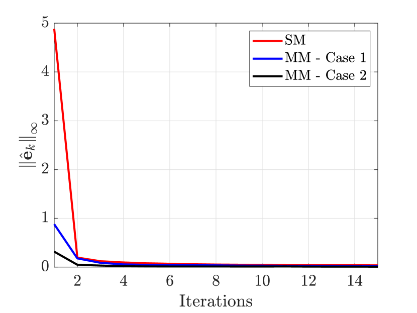
(a) Maximum Identification Error over iterations.

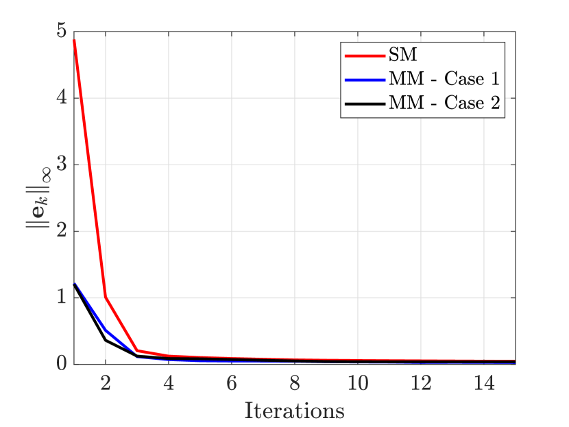
(b) Maximum Tracking Error over iterations.

Figure 1: Error profiles over iterations for an LTI system without disturbances.

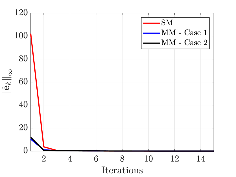
(a) Maximum Identification Error over iterations.

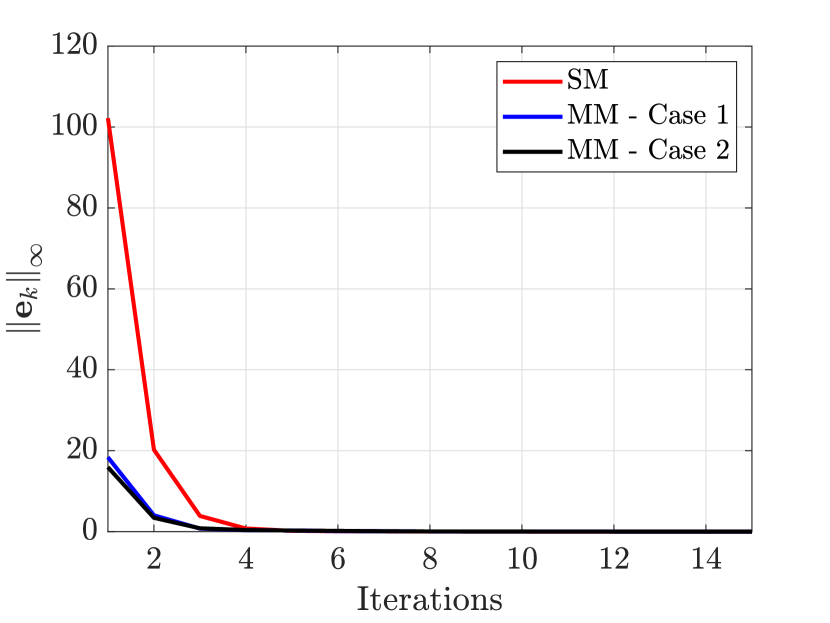
(b) Maximum Tracking Error over iterations.

Figure 2: Error profiles over iterations for an LTV system with disturbances.

5.1   Example 1: LTI System without Disturbances

Consider the system:

$$x_{k}(t+1)=0.5x_{k}(t)+u_{k}(t),$$ (45)

a simple, stable LTI system without disturbances. The objective is for $x_{k}(t)$ to track the reference $x_{m}(t)$ in (43). The results for identification and tracking performance are shown in Fig. 1, in terms of the peak amplitude of errors over iterations for each strategy. It is evident that both multiple-model strategies converge faster than the single-model strategy, mainly because the initialization of multiple estimation models leads to better estimates in earlier iterations, hence improving transient performance. Further, the multiple model strategy with criterion (27), i.e. MM - Case $2$ converges marginally faster than MM - Case $1$, due to models switching more frequently.

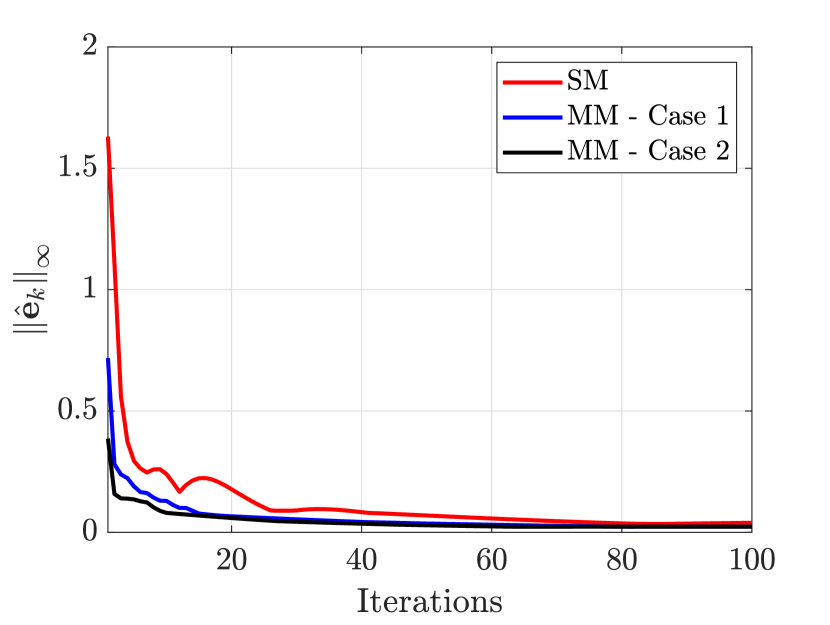
(a) Maximum Identification Error over iterations.

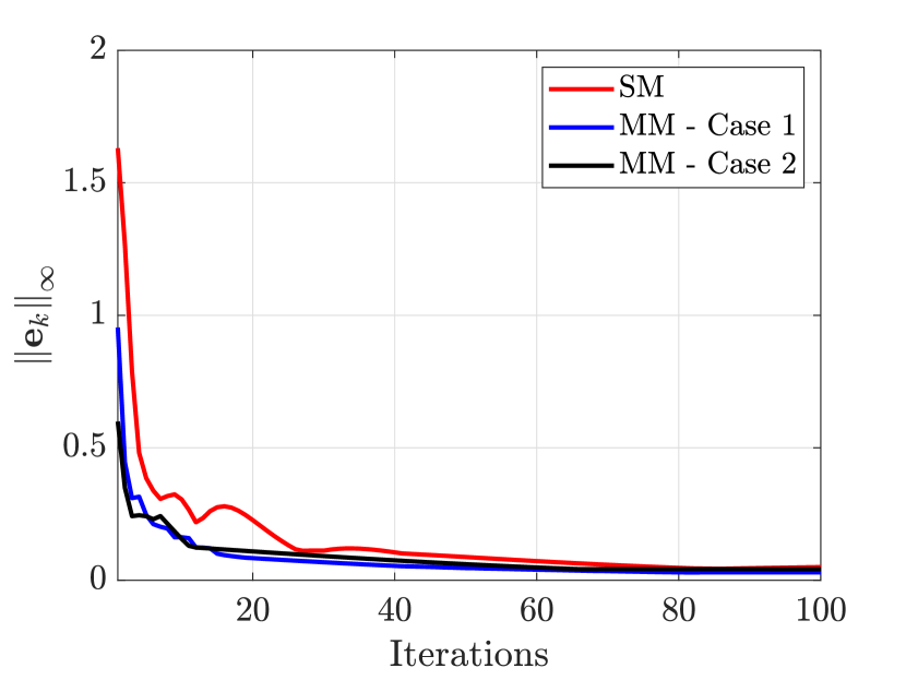
(b) Maximum Tracking Error over iterations.

Figure 3: Error profiles over iterations for a nonlinear system without disturbances.

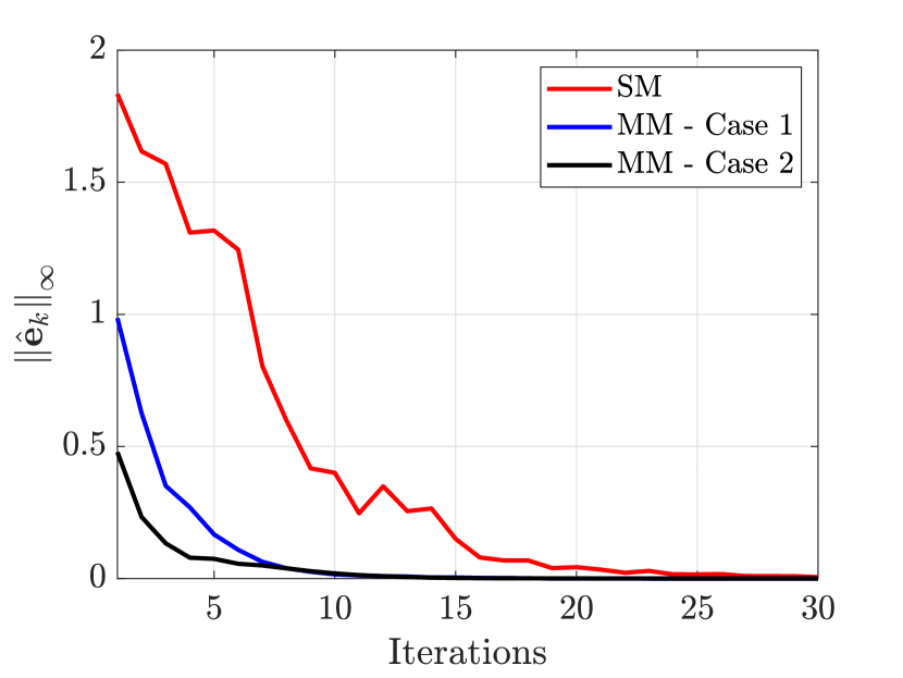
(a) Maximum Identification Error over iterations.

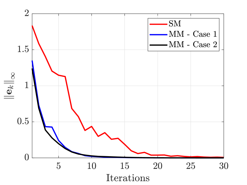
(b) Maximum Tracking Error over iterations.

Figure 4: Error profiles over iterations for a nonlinear system with disturbances.

5.2   Example 2: LTV System with Disturbances

In this example, the following LTV system with disturbances is considered:

$$x_{k}(t+1)=\theta_{1}(t)x_{k}(t)+b(t)u_{k}(t)+d(t),$$ (46)

where $\theta_{1}(t)=1+0.5\sin(t)$, $b(t)=3+0.5\sin(2\pi t)$ and $d(t)=\sin^{3}(2\pi t)$, an external disturbance. The results for achieving the tracking objective are shown in Fig. 2. As before, the two multiple-model cases achieve faster convergence due to improved transient response, whereas the single-model case has very poor transient response due to large initial parametric errors. This example also demonstrates the first instance of time-varying parameters being successfully identified over iterations.

5.3   Example 3: Nonlinear System without Disturbances

The following nonlinear system is considered:

$$x_{k}(t+1)=\theta_{1}(t)\sin^{2}\left(x_{k}(t)\right)+b(t)u_{k}(t),$$ (47)

where $\theta_{1}(t)=1+0.5\sin(t)$ and $b(t)=3+0.5\sin(2\pi t)$, as before. Note the nonlinearity in the regression vector, in contrast to the previous examples. Fig. 3 shows the results for identification and tracking performance for this system, in terms of the peak amplitude of the errors. The two multiple-model cases are seen to achieve faster convergence, and in particular, the strategy “MM - Case $2$” converges marginally faster due to higher frequency of switching.

5.4   Example 4: Nonlinear System with Disturbances

Finally, the most general system is considered:

$$x_{k}(t+1)=\theta_{1}(t)\sin^{2}\left(x_{k}(t)\right)+b(t)u_{k}(t)+d(t),$$ (48)

where $\theta_{1}(t)=1.5+0.5\sin(t)$, $b(t)=3+0.5\sin(2\pi t)$ and $d(t)=\sin^{3}(2\pi t)$, the same disturbance considered in (46). This is very similar to the system considered in [37]. Fig. 4 shows the performance for tracking the reference (43) over iterations, in terms of peak identification and tracking errors. It is evident that the convergence for both multiple-model cases is significantly faster than the single-model case, with MM - Case $2$ providing the fastest convergence. Interestingly, the errors for this system also converge faster than the errors for the system (47), which was not affected by disturbances. This is due to the presence of $d(t)$ and its estimate, resulting in a persistently exciting control law.

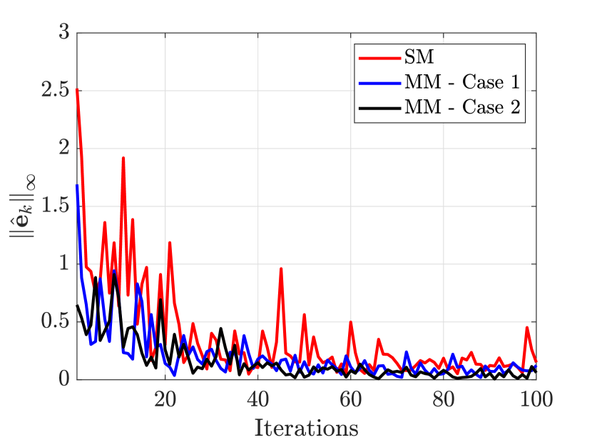
(a) Maximum Identification Error over iterations.

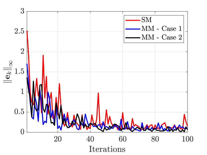
(b) Maximum Tracking Error over iterations.

Figure 5: Error profiles over iterations for a nonlinear system with disturbances, with an iteration-varying reference trajectory.

5.5   Example 5: Iteration-varying Reference Trajectory

We also present results for the system (48) tracking an iteration-varying reference trajectory:

$$x_{m,k}(t)=\vartheta(k)\pi^{2}\left(2-3\sin^{3}(2\pi t/100)\right)\sin(2\pi t/100)/10,$$ (49)

where $\vartheta(k)\sim\mathcal{U}[-0.5,0.5]$, i.e. a uniformly distributed random variable between $-0.5$ and $0.5$, in each iteration $k$. This is similar to the trajectory considered in [37]. The results for this example are shown in Fig. 5. It is easily seen that all errors are decreasing and are quite close to $0$. Further, the two multiple-model strategies are seen to perform better than the single-model strategy. To reinforce this, Table 3 presents the root-mean-square value of peak error amplitudes over iterations for identification and tracking errors for all three strategies. This metric is defined below for the identification error:

$$\mathrm{Metric}=\sqrt{\frac{1}{K}\sum_{k=1}^{K}\left\|\hat{\mathbf{e}}_{k}\right\|^{2}_{\infty}},$$ (50)

and defined similarly for the tracking error. $K$ denotes the total number of iterations in the simulation. Lower values of this metric indicate better performance. From Table 3, it is evident that both multiple-model strategies have significantly smaller values of this metric, indicating smaller identification and tracking errors and faster convergence. The smallest values are in MM - Case $2$, indicating that this strategy achieves the best possible performance. Further, Table 4 presents the number of iterations $k^{*}$ taken for tracking convergence. In particular, we consider the number of iterations taken for the peak tracking error $\left\|\mathbf{e}_{k}\right\|_{\infty}$ to fall below $2\%$ of the first iteration peak tracking error $\left\|\mathbf{e}_{1}\right\|_{\infty}$ of the single model strategy. It is once again evident that both multiple model strategies converge faster, with MM - Case $2$ converging fastest. As mentioned earlier, this is partly because the initialization of multiple estimation models leads to better estimates in earlier iterations, leading to faster convergence.

In conclusion, all simulation examples demonstrate that the proposed strategies result in convergence of identification and tracking errors to zero. The multiple model strategies converge much faster than the single model strategy, and the multiple model strategy with criterion (27) converges faster than that with criterion (26). Note how the initial error magnitudes were larger for the linear systems compared to the nonlinear systems. This is due to the presence of the nonlinearity $\sin^{2}\left(x_{k}(t)\right)$, which is always bounded between $0$ and $1$ irrespective of the value of $x_{k}(t)$. The nonlinear system subjected to disturbances also shows faster error convergence than the system without disturbances.

Table 3: Root Mean-Square Maximum Errors

Strategy	Identification Error	Tracking Error
Single Model	$6.3288$	$6.2884$
Multiple Models – Case $1$	$3.0544$	$3.4948$
Multiple Models – Case $2$	$2.0728$	$3.1338$

Table 4: Iterations for Tracking Convergence

Strategy	Number of Iterations $k^{*}$
Single Model	$79$
Multiple Models – Case $1$	$58$
Multiple Models – Case $2$	$47$

6    Concluding Remarks

In this article, we have proposed a complete framework for using the Multiple Models, Switching and Tuning (MMST) methodology in the context of discrete-time Adaptive Iterative Learning Control (ILC). First, the single estimation model case is considered, a new control and identification scheme is presented, and convergence is proved using the properties of square-summable, or $\ell_{2}$ sequences. The update law for parameter estimates uses the identification error rather than the tracking error, in contrast to existing Adaptive ILC schemes. This enables the extension to multiple estimation models. In the case of multiple models, we have described two criteria for switching between models — either at the end of each iteration or at each sample. In both options, convergence is proved in a unified manner using the properties of square-summable sequences. An extensive set of simulation results are presented for four different types of systems. In all cases, it is seen that the identification and tracking errors converge to zero. In particular, it is seen that the second switching criterion for multiple-models outperforms the first, which in turn outperforms the single model case.

A drawback of the strategies presented here is their high computational complexity, particularly for the second switching criterion (27) in multiple models. It is known that the Multiple Models with Second-Level Adaptation (MM-SLA) scheme [60, 61] has lower computational complexity compared to MMST, as a much smaller number of estimation models, is required. This was explored for Adaptive ILC in a contraction-mapping setting in [59], and an interesting avenue for future work is to explore this in the context of CEF-based Adaptive ILC. Further, as mentioned in Section 1, the techniques proposed here can be extended to the case with time- and iteration-varying parameters, and also to the case when the control direction is unknown.

References

- [1] J.-X. Xu, “A survey on iterative learning control for nonlinear systems,” International Journal of Control, vol. 84, no. 7, pp. 1275–1294, 2011.
- [2] H.-S. Ahn, Y. Chen, and K. L. Moore, “Iterative learning control: Brief survey and categorization,” IEEE Transactions on Systems, Man, and Cybernetics – Part C: Applications and Reviews, vol. 37, no. 6, pp. 1099–1121, Nov. 2007.
- [3] K. L. Moore, Iterative Learning Control for Deterministic Systems. London, United Kingdom: Springer-Verlag, 1993.
- [4] D. A. Bristow, M. Tharayil, and A. G. Alleyne, “A survey of iterative learning control,” IEEE Control Systems Magazine, vol. 26, no. 3, pp. 96–114, Jun. 2006.
- [5] Z. Bien and J.-X. Xu, Eds., Iterative Learning Control: Analysis, Design, Integration and Applications. New York, NY, USA: Springer Science + Business Media, 1998.
- [6] S. Arimoto, S. Kawamura, and F. Miyazaki, “Bettering operation of robots by learning,” Journal of Robotic Systems, vol. 1, no. 2, pp. 123–140, 1984.
- [7] Y. Chen and K. L. Moore, “An optimal design of PD-type iterative learning control with monotonic convergence,” in Proceedings of the IEEE International Symposium on Intelligent Control, Vancouver, Canada, Oct. 2002, pp. 55–60.
- [8] Y. Chen, C. Wen, and M. Sun, “A robust high-order P-type iterative learning controller using current iteration tracking error,” International Journal of Control, vol. 68, no. 2, pp. 331–342, 1997.
- [9] C.-J. Chien and J.-S. Liu, “A P-type iterative learning controller for robust output tracking of nonlinear time-varying systems,” International Journal of Control, vol. 64, no. 2, pp. 319–334, 1996.
- [10] Z. Wang, C. P. Pannier, K. Barton, and D. J. Hoelzle, “Application of robust monotonically convergent spatial iterative learning control to microscale additive manufacturing,” Mechatronics, vol. 56, pp. 157–165, Dec. 2018.
- [11] A. A. Armstrong and A. G. Alleyne, “A multi-input single-output iterative learning control for improved material placement in extrusion-based additive manufacturing,” Control Engineering Practice, vol. 111, pp. 104 783: 1–11, Jun. 2021.
- [12] A. Laracy and H. Ossareh, “Constraint management for batch processes using iterative learning control and reference governors,” in Proceedings of the 2nd Conference on Learning for Dynamics and Control, ser. Proceedings of Machine Learning Research, vol. 120, Jun. 2020, pp. 340–349.
- [13] X. Liu, L. Ma, X. Kong, and K. Lee, “Robust model predictive iterative learning control for iteration-varying-reference batch processes,” IEEE Transactions on Systems, Man and Cybernetics: Systems, vol. 51, no. 7, pp. 4238–4250, Jul. 2021.
- [14] S. Chen, Z. Wang, A. Chakraborty, M. Klecka, G. Saunders, and J. Wen, “Robotic deep rolling with iterative learning motion and force control,” IEEE Robotics and Automation Letters, vol. 5, no. 4, pp. 5581–5588, Oct. 2020.
- [15] Y. Chen, B. Chu, C. T. Freeman, and Y. Liu, “Generalized iterative learning control with mixed system constraints: A gantry robot based verification,” Control Engineering Practice, vol. 95, pp. 104 260: 1–11, Feb. 2020.
- [16] R. Mengacci, F. Angelini, M. G. Catalano, G. Grioli, A. Bicchi, and M. Garabini, “On the motion/stiffness decoupling property of articulated soft robots with application to model-free torque iterative learning control,” The International Journal of Robotics Research, vol. 40, no. 1, pp. 348–374, Jan. 2021.
- [17] M. Norrlöf and S. Gunnarsson, “Time and frequency domain convergence properties in iterative learning control,” International Journal of Control, vol. 75, no. 14, pp. 1114–1126, 2002.
- [18] H.-S. Ahn, K. L. Moore, and Y. Chen, Iterative Learning Control: Robustness and Monotonic Convergence for Interval Systems. London, United Kingdom: Springer-Verlag, 2007.
- [19] D. Wang, “Convergence and robustness of discrete time nonlinear systems with iterative learning control,” Automatica, vol. 34, no. 11, pp. 1445–1448, Nov. 1998.
- [20] H.-S. Lee and Z. Bien, “Study on robustness of iterative learning control with non-zero initial error,” International Journal of Control, vol. 64, no. 3, pp. 345–349, 1996.
- [21] Z. Shahriari, B. Bernhardsson, and O. Troeng, “Convergence analysis of iterative learning control using pseudospectra,” International Journal of Control, vol. 95, no. 1, pp. 269–281, 2022.
- [22] M. French and E. Rogers, “Non-linear iterative learning by an adaptive Lyapunov technique,” International Journal of Control, vol. 73, no. 10, pp. 840–850, 2000.
- [23] J.-X. Xu and Y. Tan, “A suboptimal learning control scheme for non-linear systems with time-varying parametric uncertainties,” Optimal Control Applications & and Methods, vol. 22, no. 3, pp. 111–126, May/Jun. 2001.
- [24] ——, “A composite energy function-based learning control approach for nonlinear systems with time-varying parametric uncertainties,” IEEE Transactions on Automatic Control, vol. 47, no. 11, pp. 1940–1945, Nov. 2002.
- [25] J.-X. Xu, “The frontiers of iterative learning control - II,” Systems, Control and Information, vol. 46, no. 5, pp. 233–243, 2002.
- [26] J.-X. Xu, Y. Tan, and T.-H. Lee, “Iterative learning control design based on composite energy function with input saturation,” in Proceedings of the 2003 American Control Conference, 2003, Denver, CO, USA, Jun. 2003, pp. 5129–5134.
- [27] A. Tayebi and C.-J. Chien, “A unified adaptive iterative learning control framework for uncertain nonlinear systems,” IEEE Transactions on Automatic Control, vol. 52, no. 10, pp. 1907–1913, Oct. 2007.
- [28] A. Tayebi, “Adaptive iterative learning control for robot manipulators,” in Proceedings of the 2003 American Control Conference, 2003, Denver, CO, USA, Jun. 2003, pp. 4518–4523.
- [29] ——, “Adaptive iterative learning control for robot manipulators,” Automatica, vol. 40, no. 7, pp. 1195–1203, Jul. 2004.
- [30] R. Lee, L. Sun, Z. Wang, and M. Tomizuka, “Adaptive iterative learning control of robot manipulators for friction compensation,” in 8th IFAC Symposium on Mechatronic Systems (MECHATRONICS) 2019, Vienna, Austria, Sep. 2019, pp. 175–180.
- [31] L. Wu, Q. Yan, and J. Cai, “Neural network-based adaptive learning control for robot manipulators with arbitrary initial errors,” IEEE Access, vol. 7, pp. 180 194–180 204, Dec. 2019.
- [32] D. Huang, Y. Chen, D. Meng, and P. Sun, “Adaptive iterative learning control for high-speed train: A multi-agent approach,” IEEE Transactions on Systems, Man and Cybernetics: Systems, vol. 51, no. 7, pp. 4067–4077, Jul. 2021.
- [33] Q. Yu and Z. Hou, “Adaptive fuzzy iterative learning control for high-speed trains with both randomly varying operation lengths and system constraints,” IEEE Transactions on Fuzzy Systems, vol. 29, no. 8, pp. 2408–2418, Aug. 2021.
- [34] G. Liu and Z. Hou, “RBFNN-based adaptive iterative learning fault-tolerant control for subway trains with actuator faults and speed constraint,” IEEE Transactions on Systems, Man and Cybernetics: Systems, vol. 51, no. 9, pp. 5785–5799, Sep. 2021.
- [35] W. He, T. Meng, S. Zhang, J.-K. Liu, G. Li, and C. Sun, “Dual-loop adaptive iterative learning control for a Timoshenko beam with output constraint and input backlash,” IEEE Transactions on Systems, Man and Cybernetics: Systems, vol. 49, no. 5, pp. 1027–1038, May 2019.
- [36] J. Feng, Z. Liu, X. He, Q. Li, and W. He, “Vibration suppression of a high-rise building with adaptive iterative learning control,” IEEE Transactions on Neural Networks and Learning Systems, pp. 1–12, 2021, early access.
- [37] R. Chi, Z. Hou, and J. Xu, “Adaptive ILC for a class of discrete-time systems with iteration-varying trajectory and random initial condition,” Automatica, vol. 44, no. 8, pp. 2207–2213, Aug. 2008.
- [38] G. C. Goodwin and K. S. Sin, Adaptive Filtering Prediction and Control. Englewood Cliffs, NJ: Prentice Hall, 1984.
- [39] R. Chi, S.-L. Sui, and Z.-H. Hou, “A new discrete-time adaptive ILC for nonlinear systems with time-varying parametric uncertainties,” Acta Automatica Sinica, vol. 34, no. 7, pp. 805–808, Jul. 2008.
- [40] M. Sun, X. Liu, and H. He, “Adaptive iterative learning control for SISO discrete time-varying systems,” in 2012 12th International Conference on Control, Automation, Robotics & Vision, Guangzhou, China, Dec. 2012, pp. 58–63.
- [41] B. Liu and W. Zhou, “On adaptive iterative learning control algorithm for discrete-time systems with parametric uncertainties subject to second-order internal model,” in 10th International Conference on Computer Science & Education (ICCSE 2015), Cambridge, United Kingdom, Jul. 2015, pp. 512–517.
- [42] M. Yu, J. Zhang, and D. Qi, “Discrete-time adaptive iterative learning control with unknown control directions,” International Journal of Control, Automation and Systems, vol. 10, no. 6, pp. 1111–1118, Dec. 2012.
- [43] M. Yu, J. Wang, and D. Qi, “Discrete-time adaptive iterative learning control for high-order nonlinear systems with unknown control directions,” International Journal of Control, vol. 86, no. 2, pp. 299–308, Feb. 2013.
- [44] W. Yan and M. Sun, “Adaptive iterative learning control of discrete-time varying systems with unknown control direction,” International Journal of Adaptive Control and Signal Processing, vol. 27, no. 4, pp. 340–348, Apr. 2012.
- [45] M. Yu, D. Huang, and W. He, “Robust adaptive iterative learning control for discrete-time nonlinear systems with both parametric and nonparametric uncertainties,” International Journal of Adaptive Control and Signal Processing, vol. 30, no. 7, pp. 972–985, Jul. 2016.
- [46] M. Yu and C. Li, “Robust adaptive iterative learning control for discrete-time nonlinear systems with time-iteration-varying parameters,” IEEE Transactions on Systems, Man and Cybernetics: Systems, vol. 47, no. 7, pp. 1737–1745, Jul. 2017.
- [47] X. Bu and Z. Hou, “Adaptive iterative learning control for linear systems with binary-valued observations,” IEEE Transactions on Neural Networks and Learning Systems, vol. 29, no. 1, pp. 232–237, Jan. 2018.
- [48] X. Yu, Z. Hou, M. M. Polycarpou, and L. Duan, “Data-driven iterative learning control for nonlinear discrete-time MIMO systems,” IEEE Transactions on Neural Networks and Learning Systems, vol. 32, no. 3, pp. 1136–1148, Mar. 2021.
- [49] Q. Yu, Z. Hou, X. Bu, and Q. Yu, “RBFNN-based data-driven predictive iterative learning control for nonaffine nonlinear systems,” IEEE Transactions on Neural Networks and Learning Systems, vol. 31, no. 4, pp. 1170–1182, Apr. 2020.
- [50] K. S. Narendra and J. Balakrishnan, “Performance improvement in adaptive control systems using multiple models and switching,” in Proceedings of the Seventh Yale Workshop on Adaptive and Learning Systems, Center for Systems Science, Yale University, New Haven, CT, USA, May 1992, pp. 27–33.
- [51] ——, “Adaptive control using multiple models,” IEEE Transactions on Automatic Control, vol. 42, no. 2, pp. 171–187, Feb. 1997.
- [52] K. S. Narendra and C. Xiang, “Adaptive control of discrete-time systems using multiple models,” IEEE Transactions on Automatic Control, vol. 45, no. 9, pp. 1669–1686, Sep. 2000.
- [53] R. Makam and K. George, “Convex combination of multiple models for discrete-time adaptive control,” International Journal of Systems Science, vol. 53, no. 4, pp. 743–756, 2022.
- [54] ——, “Multiple models for decentralized control of discrete-time adaptive systems,” (Submitted), pp. 1–10, 2021.
- [55] L. Xiaoli and Z. Wen, “Multiple model iterative learning control,” Neurocomputing, vol. 73, no. 13–15, pp. 2439–2445, Aug. 2012.
- [56] X. Li, K. Wang, and D. Liu, “An improved result of multiple model iterative learning control,” IEEE/CAA Journal of Automatica Sinica, vol. 1, no. 3, pp. 315–322, Jul. 2014.
- [57] C. Freeman and M. French, “Estimation based multiple model iterative learning control,” in 2015 54th IEEE Conference on Decision and Control (CDC), Osaka, Japan, Dec. 2015, pp. 6070–6075.
- [58] R. Padmanabhan, M. Bhushan, K. K. Hebbar, R. Makam, and K. George, “A novel strategy with multiple models to improve performance of adaptive iterative learning control,” in 2021 IEEE International Conference on Electronics, Computing and Communication Technologies (CONECCT), Bengaluru, India, Jul. 2021.
- [59] ——, “Second-level adaptation and optimization for multiple model adaptive iterative learning control,” in 2021 Seventh Indian Control Conference (ICC), Mumbai, India, Dec. 2021.
- [60] K. S. Narendra and Z. Han, “Discrete-time adaptive control using multiple models,” in Proceedings of the 2011 American Control Conference, San Francisco, CA, USA, Jun.-Jul. 2011, pp. 2921–2926.
- [61] R. Makam, S. Ramaiah, and K. George, “Stability analysis of deterministic discrete-time adaptive systems with second level adaptation,” in 2018 International Conference on Signals and Systems (ICSigSys), Bali, Indonesia, May 2018, pp. 167–173.
- [62] T.-H. Lee and K. S. Narendra, “Stable discrete adaptive control with unknown high-frequency gain,” IEEE Transactions on Automatic Control, vol. 31, no. 5, pp. 477–479, May 1986.
- [63] Y. Qi, H. Geng, and N. Xing, “Adaptive learning control for triggered switched systems based on unknown direction control gain function,” International Journal of Control, pp. 1–12, 2022, early access.