Hydromagnetic waves in an expanding universe – cosmological MHD code tests using analytic solutions

Abstract

We describe how analytic solutions for linear hydromagnetic waves can be used for testing cosmological magnetohydrodynamic (MHD) codes. We start from the comoving MHD equations and derive analytic solutions for the amplitude evolution of linear hydromagnetic waves in a matter-dominated, flat Einstein-de-Sitter (EdS) universe. The waves considered are comoving, linearly polarized Alfvén waves and comoving, magnetosonic (fast) waves modified by self-gravity. The solution for compressible waves is found for a general adiabatic index and we consider the limits of hydrodynamics without self-gravity in addition to the full solution. In addition to these analytic solutions, the linearized equations are solved numerically for a $\Lambda$CDM cosmology. We use the analytic and numeric solutions to compare with results obtained using the cosmological MHD code arepo and find good agreement when using a sufficient number of grid points. We interpret the numerical damping clearly evident in simulations with few grid points by further deriving the Alfvén wave solution including physical Navier-Stokes viscosity. A comparison between Alfvén wave simulations and theory reveals that the dissipation can be described by a numerical viscosity coefficient $\eta_{\mathrm{num}}\propto a^{-5/2}$ where $a$ is the scale factor. We envision that our examples could be useful when developing a new cosmological MHD code or for regression testing of existing codes.

1 Introduction

Cosmological computer codes play an increasingly central role in theoretical astrophysics. In their most basic state, these codes typically couple a gravitational solver for dark matter with a hydrodynamic description of the baryonic gas (e.g. Evrard 1988; Springel 2005; Teyssier 2002; Springel 2010; Bryan et al. 2014). In addition, many modern cosmological computer simulations also include physical processes such as cooling, star formation and feedback from supernovae, stellar winds and AGN (see Vogelsberger et al. 2020 for a review and an extensive list of physical processes typically included). While some of these physical processes are included with phenomenological implementations, several different codes have nevertheless managed to produce galaxies with realistic properties (Somerville & Davé, 2015).

In recent years, many cosmological simulations have also begun to include magnetic fields by solving the equations of ideal magnetohydrodynamics (MHD, see e.g. Freidberg 2014). Cosmological codes with this capability include CosmoMHD (Li et al., 2008), MHD GADGET (Dolag & Stasyszyn, 2009), enzo (Collins et al., 2010; Bryan et al., 2014), arepo (Springel, 2010; Pakmor & Springel, 2013), gizmo (Hopkins & Raives, 2016), ramses (Dubois & Teyssier, 2008; Rieder & Teyssier, 2017), wombat (Mendygral et al., 2017), GCMHD++ (Barnes et al., 2018), and masclet (Quilis et al., 2020). These cosmological codes use comoving coordinates which follow the expansion of the universe. The transformation to comoving coordinates transforms the standard MHD equations into the comoving MHD equations. The comoving version differs from the standard version by having factors of $a$ and $\dot{a}$ where $a$ is the scale factor and $\dot{a}$ is its time derivative. Despite this difference, only minor modifications of the algorithms used for standard MHD are required to solve the comoving MHD equations (e.g. Pakmor & Springel 2013).

Examples of simulations performed with comoving MHD codes include ’universe-in-a-box’ simulations (e.g. Marinacci et al. 2018; Hopkins et al. 2018; Katz et al. 2021; Garaldi et al. 2021) and ’zoom’ simulations which for instance aim to understand the role of magnetic fields in isolated or merging galaxies (e.g. Pakmor et al. 2014; Whittingham et al. 2021), the circumgalactic medium of galaxies (e.g. Pakmor et al. 2020; van de Voort et al. 2021) or galaxy clusters (e.g. Dolag et al. 1999; Vazza et al. 2018; Quilis et al. 2020).

An essential ingredient in building trust in the results of such computer simulations is verifying that the computer code used performs well on a number of well-defined test problems. Many such tests are known from standard MHD (e.g. Stone et al. 2008) but very few have been developed specifically for comoving MHD (see Appendix A for a brief review of these).

Due to the similarities between standard and comoving MHD, cosmological codes are therefore mainly verified using tests developed for standard MHD. This is normally done by simply setting $a=1$ and $\dot{a}=0$ in the comoving MHD codes. This could be problematic because it makes it possible for errors related to $a\neq 1$ and $\dot{a}\neq 0$ to go unnoticed. Since such errors could have far-reaching consequences for the validity of simulation results, we advocate in this paper for introducing additional tests that specifically target the comoving MHD equations.

We argue that the test cases should ideally have analytic solutions or, when this is not possible, have high-precision reference solutions which can be universally agreed upon. In addition, it is useful if the tests are computationally cheap since this encourages frequent testing. Hydromagnetic waves in comoving coordinates fulfill these requirements because i) analytic solutions can be derived and ii) wave motion can be simulated in one spatial dimension (1D) such that tests can be done within a few minutes on most personal computers. The purpose of this paper is therefore to provide analytic reference solutions for hydromagnetic waves and to give practical examples of how they can be used to test comoving MHD implementations.

The rest of the paper is divided as follows: we first introduce the equations of ideal MHD and their comoving counterpart in Section 2. We then derive analytic wave solutions in Einstein-de-Sitter (EdS) cosmology in Section 3. In particular, Section 3.4 contains the comoving Alfvén wave derivation while Section 3.5 contains the derivation of analytic solutions for comoving magnetosonic waves modified by self-gravity. Moving beyond EdS, we also provide a brief description of a procedure for numerically solving the linearized equations for a $\Lambda$CDM cosmology in Section 4. These analytic and numeric reference solutions are used to test the comoving MHD code arepo in Section 5. The test section is divided into subsections describing Alfvén wave tests (Section 5.1) and compressible wave tests (Section 5.2). These test cases consider both standing and traveling waves as well as their convergence properties. We discuss the effects of self-gravity and magnetic fields on the compressible waves and how changing the adiabatic index leads to interesting behaviour. We conclude the paper by discussing the merits of code testing in Section 6. Finally, the paper also contains three appendices which provide brief outlines of the code tests currently in use for comoving MHD (Appendix A), the transformation from standard MHD to comoving MHD (Appendix B) and additional details about the analytic solutions (Appendix C).

2 Comoving MHD equations with self-gravity

We start by introducing the equations of standard MHD and their comoving counterpart. We take $\bm{r}$ to be the spatial coordinate in a fixed coordinate system and $\bm{x}$ to be the comoving coordinate. These are related by $\bm{r}=a\bm{x}$ where $a$ is the time-dependent cosmological scale factor which evolves according to the Friedmann equation

$$\dot{a}=aH_{0}\left(\frac{\Omega_{\mathrm{m},0}}{a^{3}}+\frac{\Omega_{\mathrm{r},0}}{a^{4}}+\Omega_{\Lambda,0}\right)^{1/2}\ ,$$ (1)

where $H_{0}$ is the Hubble parameter and $\Omega_{\mathrm{m},0}$, $\Omega_{\mathrm{r},0}$, and $\Omega_{\Lambda,0}$ are the $z=0$ values of the cosmological parameters for total density (baryonic plus dark matter), radiation and dark energy, respectively. Cosmological MHD simulations generally start at redshifts low enough that the radiation density can effectively be ignored. We therefore set $\Omega_{\mathrm{r},0}=0$ throughout the paper.

The standard (i.e. non-comoving) equations of ideal MHD are the mass continuity, momentum, induction and entropy equations. In Heaviside-Lorentz units, they are given by (e.g. Freidberg 2014)

$$\frac{d\ln\rho}{dt}=-\nabla_{\bm{r}}\mbox{\boldmath{$\cdot$}}\bm{\varv}\ ,$$ (2)

$$\rho\frac{d\bm{\varv}}{dt}=-\nabla_{\bm{r}}p-\nabla_{\bm{r}}\mbox{\boldmath{$\cdot$}}\left(\frac{B^{2}}{2}\mathbf{1}-\bm{B}\bm{B}\right)-\rho\nabla_{\bm{r}}\Phi\ ,$$ (3)

$$\frac{\partial{\bm{B}}}{\partial{t}}=\nabla_{\bm{r}}\times\left(\bm{\varv}\times\bm{B}\right)\ ,$$ (4)

$$\frac{p}{\gamma-1}\frac{d\ln\left(p\rho^{-\gamma}\right)}{dt}=0\ ,$$ (5)

where $d/dt=\partial/\partial t+\bm{\varv}\mbox{\boldmath{$\cdot$}}\nabla_{\bm{r}}$ is the convective derivative with $\partial/\partial t$ taken at fixed position $\bm{r}$, $\rho$ is the gas density, $\bm{\varv}$ is the gas velocity, $p$ is the thermal pressure, $\bm{B}$ is the magnetic field vector with strength $B$, $\mathbf{1}$ is the unit tensor, $\bm{B}\bm{B}$ is a dyadic product, $\Phi$ is the gravitational potential and $\gamma$ is the adiabatic index. We also note that the entropy equation can equivalently be written as

$$\frac{d\ln\varepsilon}{dt}=-\gamma\nabla_{\bm{r}}\mbox{\boldmath{$\cdot$}}\bm{\varv}\ ,$$ (6)

where $\varepsilon=p/(\gamma-1)$ is the internal energy.

The comoving MHD equations can be derived by transforming from the $\bm{r}$ coordinate system to the $\bm{x}$ coordinate system and including a cosmological source term in Poisson’s equation for the gravitational potential. We provide a brief outline of a derivation in Appendix B. The result is

$$\frac{d\ln\rho_{\mathrm{c}}}{dt}=-\frac{1}{a}\nabla_{\bm{x}}\mbox{\boldmath{$\cdot$}}\bm{u}\ ,$$ (7)

$$a\rho_{\mathrm{c}}\frac{d\bm{u}}{dt}=-\nabla_{\bm{x}}p_{\mathrm{c}}-\frac{1}{a}\nabla_{\bm{x}}\mbox{\boldmath{$\cdot$}}\left(\frac{B_{\mathrm{c}}^{2}}{2}\mathbf{1}-\bm{B}_{\mathrm{c}}\bm{B}_{\mathrm{c}}\right)-\rho_{\mathrm{c}}\nabla_{\bm{x}}\delta\Phi-\rho_{\mathrm{c}}\dot{a}\bm{u}\,,$$ (8)

$$\frac{\partial{\bm{B}_{\mathrm{c}}}}{\partial{t}}=\frac{1}{a}\nabla_{\bm{x}}\times\left(\bm{u}\times\bm{B}_{\mathrm{c}}\right)\ ,$$ (9)

$$\frac{d\varepsilon_{\mathrm{c}}}{dt}=-3\frac{\dot{a}}{a}\left(\gamma-1\right)\varepsilon_{\mathrm{c}}-\gamma\varepsilon_{\mathrm{c}}\frac{1}{a}\nabla_{\bm{x}}\mbox{\boldmath{$\cdot$}}\bm{u}\ ,$$ (10)

and

$$\nabla_{\bm{x}}^{2}\delta\Phi=\frac{4\pi G}{a}\delta\rho_{\mathrm{tot,c}}\ ,$$ (11)

where $d/dt=\partial/\partial t+a^{-1}\bm{u}\mbox{\boldmath{$\cdot$}}\nabla_{\bm{x}}$ is the convective derivative with $\partial/\partial t$ taken at fixed position $\bm{x}$, $\rho_{\mathrm{c}}=\rho a^{3}$ is the comoving gas density, $\bm{u}$ is the peculiar velocity, $\bm{B}_{\mathrm{c}}=\bm{B}a^{2}$ is the comoving magnetic field and $\varepsilon_{\mathrm{c}}=\varepsilon a^{3}$ is the comoving internal energy. The density sourcing the Poisson equation is $\delta\rho_{\mathrm{tot,c}}=\left(\rho_{\mathrm{tot,c}}-\bar{\rho}_{\mathrm{tot,c}}\right)$ where $\rho_{\mathrm{tot,c}}$ is the comoving total density (baryons, dark matter etc) and $\bar{\rho}_{\mathrm{tot,c}}$ is its mean (see details in Appendix B).

3 Analytic solutions

We derive analytic solutions for comoving MHD waves by using linear perturbation theory. Our derivation is related to the extensive literature on cosmological perturbation theory which we discuss below.

The compressible modes in a hydrodynamic fluid coupled to self-gravity is a well-known problem which is treated in most textbooks on cosmology (e.g. chapter 16 in Peebles 1980). Most textbooks, e.g. Cimatti et al. (2019), have a focus on scales that are dominated by gravitational instability. They therefore assume that the thermal pressure gradient can be neglected which has the advantage that it significantly simplifies the problem. In order to study stable hydrodynamic waves modified by gravity it is however essential that the pressure gradient is retained. This is done in the book by Weinberg 1972 which discusses the Bessel function solution that then arises.

Moving beyond hydrodynamics is motivated by the belief that the early Universe contained primordial magnetic fields (Grasso & Rubinstein, 2001; Durrer & Neronov, 2013; Subramanian, 2016). The extension to MHD was pioneered by Wasserman (1978) who considered magnetic fields in the limit of zero thermal pressure gradient. It was shown that magnetic fields can create density perturbations which could seed gravitational instability with consequences for large-scale structure formation. This idea has since been further developed by e.g. Kim et al. (1996), Tsagas & Maartens (2000), Gopal & Sethi (2003), and Shaw & Lewis (2012).

Hydromagnetic waves in the early universe have also been extensively studied in the context of the cosmic microwave background (CMB, Planck Collaboration et al. 2016, 2020). Such studies generally include a variety of physical effects beyond ideal MHD which are believed to be important prior to recombination ($z\sim 1100$). For instance, Jedamzik et al. (1998) and Subramanian & Barrow (1998) considered neutrino and photon damping of Alfvén and magnetosonic waves. It is also common to consider a spectrum of waves since this makes a connection to observations (Subramanian, 2006; Shaw & Lewis, 2012).

Other relevant work includes Holcomb & Tajima (1989) who studied waves in a radiation-dominated cosmology in the ultra-relativistic limit and a follow-up work which considered a post-recombination plasma in a matter-dominated universe (Holcomb, 1990). These works were extended by Sil et al. (1996) who considered a general $\gamma$ and a cosmology parametrized by $a\propto t^{n}$ where $n$ is a free parameter (e.g. $n=2/3$ for a matter-dominated universe and $n=1/2$ for a radiation-dominated universe).

The by far most comprehensive study of MHD waves in an expanding universe was given by Gailis et al. (1994); Gailis et al. (1995) who derived the MHD eigenmodes for a general orientation of the magnetic field and wave vector. Given the breadth of their analysis, we find it likely that some of our analytic results can be shown to be special cases of their non-relativistic, matter-dominated solutions. However, we note that Gailis et al. (1995) did not include self-gravity and that they focused on $\gamma=4/3$ and $5/3$. This is in contrast to our magnesonic wave solution which considers a simple geometry but includes self-gravity and allows for a general adiabatic index.

3.1 Spatially uniform and motionless background

Linear perturbation theory requires a background on which to perturb. We detail this background here. We consider a universe which has no peculiar motions and is spatially uniform (i.e. $\bm{u}$ and all gradients of the background are zero). It can be seen that the right-hand sides (RHSs) of equations (7)–(10) are all zero for such a background when $\gamma=1$. The (well-known) consequence is that the background stays constant in time for such isothermal systems. For non-isothermal systems, e.g. adiabatic with $\gamma=5/3$, the internal energy decays during cosmic expansion. This can be seen directly from the non-zero RHS of equation (10). The equation can be integrated to reveal that the comoving pressure, $p_{\mathrm{c}}=\varepsilon_{\mathrm{c}}(\gamma-1)$ evolves as

$$p_{\mathrm{c}}(a)=p_{\mathrm{c}}(a_{\mathrm{i}})\,\left(\frac{a}{a_{\mathrm{i}}}\right)^{-3(\gamma-1)}=\frac{p_{\mathrm{c},0}}{\,a^{3(\gamma-1)}}\$$ (12)

where $a_{\mathrm{i}}$ is the initial scale factor, $p_{\mathrm{c}}(a_{\mathrm{i}})$ is the comoving pressure at $a_{\mathrm{i}}$ and $p_{\mathrm{c},0}$ is the comoving pressure at $z=0$ (here the redshift, $z$, is related to the scale factor by $a=1/(z+1)$ with $a=1$ at $z=0$).

3.2 Characteristic wave speed and frequency definitions

We define the adiabatic sound speed $c_{\mathrm{s}}=\sqrt{\gamma p/\rho}$ and the Alfvén speed $\varv_{\mathrm{A}}=B/\sqrt{\rho}$. With $B=B_{\mathrm{c}}a^{-2}$, $\rho=\rho_{\mathrm{c}}a^{-3}$, $p=p_{\mathrm{c}}a^{-3}$ and $p_{\mathrm{c}}=p_{\mathrm{c},0}a^{-3(\gamma-1)}$ their dependencies on redshift are given by

$$c_{\mathrm{s}}\equiv\sqrt{\frac{\gamma p}{\rho}}=\sqrt{\frac{\gamma p_{\mathrm{c},0}}{\rho_{\mathrm{c}}}}a^{-3(\gamma-1)/2}\ ,$$ (13)

and

$$\varv_{\mathrm{A}}\equiv\frac{B}{\sqrt{\rho}}=\frac{B_{\mathrm{c}}}{\sqrt{\rho_{\mathrm{c}}}}a^{-1/2}\ ,$$ (14)

respectively. We note that the sound speed depends on redshift when $\gamma\neq 1$ but that it is independent of redshift for an isothermal equation of state with $\gamma=1$. The Alfvén speed always depends on redshift. We also define a characteristic velocity

$$\varv_{\mathrm{g}}=\frac{\sqrt{4\pi G\rho_{\mathrm{c}}}}{k}a^{-1/2}\ ,$$ (15)

which is associated with the self-gravity of the gas (here $k$ is the comoving wavenumber of the wave). We observe that $\varv_{\mathrm{g}}$ and $\varv_{\mathrm{A}}$ have the same redshift dependence.

We have found it useful to introduce $\mathcal{V}_{\mathrm{s}}$, $\mathcal{V}_{\mathrm{A}}$ and $\mathcal{V}_{\mathrm{g}}$ for the values of $c_{\mathrm{s}}$, $\varv_{\mathrm{A}}$ and $\varv_{\mathrm{g}}$ at $z=0$ ($a=1$). These are given by

$$\mathcal{V}_{\mathrm{s}}\equiv\sqrt{\frac{\gamma p_{\mathrm{c},0}}{\rho_{\mathrm{c}}}}\ ,\quad\mathcal{V}_{\mathrm{A}}\equiv\frac{B_{\mathrm{c}}}{\sqrt{\rho_{\mathrm{c}}}}\ ,\quad\mathcal{V}_{\mathrm{g}}\equiv\frac{\sqrt{4\pi G\rho_{\mathrm{c}}}}{k}\ .$$ (16)

Finally, we define corresponding dimensionless frequencies

$$\Omega_{\mathrm{s}}\equiv\frac{k\mathcal{V}_{\mathrm{s}}}{H_{0}}\ ,\quad\Omega_{\mathrm{A}}\equiv\frac{k\mathcal{V}_{\mathrm{A}}}{H_{0}}\ ,\quad\Omega_{\mathrm{g}}\equiv\frac{k\mathcal{V}_{\mathrm{g}}}{H_{0}}\ ,$$ (17)

which will be used to further simplify the analytic results.

3.3 Transformations and the EdS solution

We have found it convenient to work with the scale factor, $a$, instead of the time, $t$. The transformation rule between time derivatives and scale factor derivatives is

$$\frac{\partial{f}}{\partial{t}}=\dot{a}\frac{\partial{f}}{\partial{a}}\ ,$$ (18)

where $f$ is some function. Our analytic solutions assume a flat, matter-dominated Einstein-de-Sitter (EdS) Universe in which $\Omega_{\mathrm{m},0}=1$ and $\Omega_{\mathrm{r},0}=\Omega_{\Lambda,0}=0$. It then follows from equation (1) that $\dot{a}=H_{0}/\sqrt{a}$ which allows for analytic progress.

3.4 Comoving Alfvén wave

We consider a linearly polarized comoving Alvén wave in EdS cosmology. This type of wave is incompressible and neither equation (7) nor equation (10) enters the dynamics. The linearized versions of the remaining equations, equations (8) and (9), are given by

$$\frac{\partial{}}{\partial{t}}\frac{\delta B_{\mathrm{c}}}{B_{\mathrm{c}}} = \frac{\mathrm{i}k}{a}\delta u\ ,$$ (19)

$$\frac{\partial{(a\delta u)}}{\partial{t}} = \mathrm{i}k\frac{B_{\mathrm{c}}^{2}}{a\rho_{\mathrm{c}}}\frac{\delta B_{\mathrm{c}}}{B_{\mathrm{c}}}\ ,$$ (20)

where we have taken the mean field to be in the $x$-direction and $\delta u$ and $\delta B_{\mathrm{c}}$ to be in the $y$-direction. We transform the time-derivatives to $a$-derivatives, substitute $\dot{a}=H_{0}/\sqrt{a}$ as appropriate for EdS cosmology (see equation 1), and obtain

$$\frac{\partial{}}{\partial{a}}\frac{\delta B_{\mathrm{c}}}{B_{\mathrm{c}}}=\frac{\mathrm{i}k}{H_{0}a^{1/2}}\delta u\ ,$$ (21)

$$\frac{\partial{(a\delta u)}}{\partial{a}}=\frac{\mathrm{i}k\mathcal{V}_{\mathrm{A}}^{2}}{H_{0}a^{1/2}}\frac{\delta B_{\mathrm{c}}}{B_{\mathrm{c}}}\ .$$ (22)

We solve this coupled set of equations by combining them

$$\frac{\partial{}}{\partial{a}}\left(a^{3/2}\frac{\partial{}}{\partial{a}}\frac{\delta B_{\mathrm{c}}}{B_{\mathrm{c}}}\right)=\frac{\mathrm{i}k}{H_{0}}\frac{\partial{(a\delta u)}}{\partial{a}}=-\frac{k^{2}\mathcal{V}_{\mathrm{A}}^{2}}{H_{0}^{2}a^{1/2}}\frac{\delta B_{\mathrm{c}}}{B_{\mathrm{c}}}\ ,$$ (23)

moving everything to the left-hand side (LHS) and dividing through by $a^{3/2}$. This yields the second-order ordinary differential equation (ODE) for $\delta B_{\mathrm{c}}/B_{\mathrm{c}}$

$$\frac{\partial^{2}{}}{\partial{a}^{2}}\frac{\delta B_{\mathrm{c}}}{B_{\mathrm{c}}}+\frac{3}{2a}\frac{\partial{}}{\partial{a}}\frac{\delta B_{\mathrm{c}}}{B_{\mathrm{c}}}+\frac{\Omega_{\mathrm{A}}^{2}}{a^{2}}\frac{\delta B_{\mathrm{c}}}{B_{\mathrm{c}}}=0\ ,$$ (24)

where $\Omega_{\mathrm{A}}=k\mathcal{V}_{\mathrm{A}}/H_{0}$ was defined in equation (17).

Equation (24) is an Euler differential equation and thus has a known analytic solution. We solve the indicial equation (see e.g. Asmar 2010 pages A24-A25) and find the solution

$$\frac{\delta B_{\mathrm{c}}}{B_{\mathrm{c}}}=a^{-1/4}\left(c_{1}\mathrm{e}^{\mathrm{i}\kappa\ln a}+c_{2}\mathrm{e}^{-\mathrm{i}\kappa\ln a}\right)\ ,$$ (25)

where $c_{1}$ and $c_{2}$ are integration constants and we have defined

$$\kappa\equiv\sqrt{\Omega_{\mathrm{A}}^{2}-\frac{1}{16}}\ .$$ (26)

The solution for the peculiar velocity perturbation, $\delta u$, is found by differentiation using equation (21) and (25), this yields

$$\frac{\delta u}{\mathcal{V}_{\mathrm{A}}} = -\frac{\mathrm{i}}{\Omega_{\mathrm{A}}}\sqrt{a}\frac{\partial{}}{\partial{a}}\frac{\delta B_{\mathrm{c}}}{B_{\mathrm{c}}}=\frac{\mathrm{i}}{\Omega_{\mathrm{A}}}a^{-3/4}\times$$ (27)

$$\left[c_{1}\left(\frac{1}{4}-\mathrm{i}\kappa\right)\mathrm{e}^{\mathrm{i}\kappa\ln a}+c_{2}\left(\frac{1}{4}+\mathrm{i}\kappa\right)\mathrm{e}^{-\mathrm{i}\kappa\ln a}\right]\ .$$

The integration constants can be found using prescribed initial conditions (i.e. the initial amplitudes in $\delta B_{\mathrm{c}}$ and $\delta u$) defined as $A_{B}\equiv\delta B_{\mathrm{c}}(a_{\mathrm{i}})/B_{\mathrm{c}}$ and $A_{u}\equiv\delta u(a_{\mathrm{i}})/\mathcal{V}_{\mathrm{A}}$. This is done by solving two equations for two unknowns which gives the result

$$\frac{\delta B_{\mathrm{c}}}{B_{\mathrm{c}}}=\left(\frac{a}{a_{\mathrm{i}}}\right)^{-1/4}\left[A_{B}\cos(\psi)+\frac{A_{B}+4\mathrm{i}\Omega_{\mathrm{A}}\sqrt{a_{\mathrm{i}}}A_{u}}{4\kappa}\sin(\psi)\right]\ ,$$ (28)

$$\frac{\delta u}{\mathcal{V}_{\mathrm{A}}}=\left(\frac{a}{a_{\mathrm{i}}}\right)^{-3/4}\left[A_{u}\cos\left(\psi\right)-\frac{A_{u}-4\mathrm{i}\Omega_{\mathrm{A}}a_{\mathrm{i}}^{-1/2}A_{B}}{4\kappa}\sin\left(\psi\right)\right]\ ,$$ (29)

where we have defined

$$\psi=\kappa\ln\left({a}/{a_{\mathrm{i}}}\right)\ .$$ (30)

We show the solution for $A_{B}=0$, $A_{u}=1$ in Fig. 1.

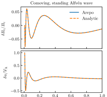
Figure 1: Standing Alfvén wave in EdS cosmology (Sections 3.4 and 5.1.1). The analytic solution is given by equations (28) and (29) (Fourier amplitudes) and in equations (75) and (76) (real space with $\delta B_{\mathrm{c}}(a_{\mathrm{i}})=0$).

The solution for a comoving Alfvén wave in EdS cosmology has many interesting features compared to the standard Alfvén wave. We make the following observations: The first, and perhaps rather obvious, observation, is that the comoving Alfvén wave decays in amplitude during cosmic expansion. Next, we observe that the Alfvén wave solution is periodic in $\ln a$, a feature also found for a shear Alfvén wave (Holcomb, 1990). In addition, the comoving Alfvén wave cannot travel at all if the background magnetic field is too weak or the wavelength is too large (Holcomb, 1990; Gailis et al., 1995). Indeed, $\kappa$ becomes imaginary when $\Omega_{\mathrm{A}}<1/4$, such that the solutions given in equations (28) and (29) turn into power law decays.

Finally, we can calculate the frequency of the comoving Alfvén wave. Taking the time derivative of the phase $\psi$ (see equation 30), we find

$$\dot{\psi}=k\mathcal{V}_{\mathrm{A}}a^{-3/2}\sqrt{1-\left(\frac{H_{0}}{4k\mathcal{V}_{\mathrm{A}}}\right)^{2}}\ ,$$ (31)

where we have used that $\dot{a}/a=H_{0}a^{-3/2}$ for EdS cosmology. We compare this to the standard Alfvén wave frequency $\omega_{\mathrm{A}}=k^{\prime}\varv_{\mathrm{A}}$ where $k^{\prime}$ is the physical wavenumber and $\varv_{\mathrm{A}}$ is the Alfvén speed. Since the wavenumber and Alfvén speed decrease as $k^{\prime}=k/a$ and $\varv_{\mathrm{A}}=\mathcal{V}_{\mathrm{A}}a^{-1/2}$ during cosmic expansion, the standard MHD theory predicts that the Alfvén frequency decreases as $\omega_{\mathrm{A}}\propto a^{-3/2}$. This $a^{-3/2}$ scaling is indeed seen in equation (31). The additional square root dependence shows that the comoving Alfvén waves are dispersive, i.e., that $\dot{\psi}/k$ depends on $k$. This modification of the wave frequency, and thus the dispersion effect, is most significant for waves close to the damping scale given by $\Omega_{\mathrm{A}}\leq 1/4$. Indeed, this dispersion feature is closely related to the damping of the wave, with the frequency of the wave going to zero as the damping becomes maximal. While the damping is here due to cosmic expansion, a similar relation between damping and dispersion is generally found for dissipative waves (see e.g. Berlok et al. 2020 for waves damped by Braginskii viscosity).

The solution given by equations (28) and (29) works well for comparing with simulations where arbitrary values of $A_{B}$ and $A_{u}$ are initialized. However, a wave eigenmode has a specific value of $A_{B}/A_{u}$. We require this eigenmode as we also wish to initialize a traveling wave in the code testing section. We therefore determine the eigenmode and thus $A_{B}/A_{u}$ as follows: the plus and minus in $\mathrm{e}^{\pm\mathrm{i}\kappa\ln a}$ in equation (25) correspond to waves traveling in opposite directions. We can without loss of generality focus on the plus solution, for which we observe that both $\delta B_{\mathrm{c}}/B_{\mathrm{c}}a^{1/4}$ and $\delta u/\mathcal{V}_{\mathrm{A}}a^{3/4}$ are proportional to $\mathrm{e}^{\mathrm{i}\kappa\ln a}$. Using this information, we can write equations (21) and (22) as an eigenvalue problem

$$\left(\begin{matrix}-\mathrm{i}/4-\kappa&\Omega_{\mathrm{A}}\\ \Omega_{\mathrm{A}}&\mathrm{i}/4-\kappa\end{matrix}\right)\left(\begin{matrix}\delta B_{\mathrm{c}}/B_{\mathrm{c}}a^{1/4}\\ \delta u/\mathcal{V}_{\mathrm{A}}a^{3/4}\end{matrix}\right)=\left(\begin{matrix}0\\ 0\end{matrix}\right)\ ,$$ (32)

where $\kappa$ is the eigenvalue. Solving this eigenvalue problem, we find the eigenmode solutions

$$\frac{\delta B_{\mathrm{c}}}{B_{\mathrm{c}}} = C\frac{\pm 4\kappa-\mathrm{i}}{4\Omega_{\mathrm{A}}}a^{-1/4}\mathrm{e}^{\pm\mathrm{i}\kappa\ln a}\ ,$$ (33)

$$\frac{\delta u}{\mathcal{V}_{\mathrm{A}}} = Ca^{-3/4}\mathrm{e}^{\pm\mathrm{i}\kappa\ln a}\ ,$$ (34)

where $C$ is the overall mode amplitude. The eigenmode thus has $A_{B}/A_{u}=\sqrt{a_{\mathrm{i}}}(\pm 4\kappa-\mathrm{i})/4\Omega_{\mathrm{A}}$.

3.5 Comoving magnetosonic wave with self-gravity

We derive analytic solutions for comoving magnetosonic waves modified by self-gravity in EdS cosmology. We take the background magnetic field and its perturbation, $\delta B_{\mathrm{c}}$, to be in the $z$-direction and the wave vector and the velocity perturbation, $\delta u$, to be in the $x$-direction. The linearized gas density equation, equation (7), is

$$\frac{\partial{}}{\partial{t}}\frac{\delta\rho_{\mathrm{c}}}{\rho_{\mathrm{c}}}=-\frac{\mathrm{i}k}{a}\delta u\ ,$$ (35)

the linearized momentum equation, equation (8), is

$$\frac{\partial{(a\delta u)}}{\partial{t}}=-\mathrm{i}k\left(\frac{\delta p_{\mathrm{c}}}{\rho_{\mathrm{c}}}-\frac{4\pi G\rho_{\mathrm{c}}}{k^{2}a}\frac{\delta\rho_{\mathrm{c}}}{\rho_{\mathrm{c}}}+\frac{B_{\mathrm{c}}^{2}}{a\rho_{\mathrm{c}}}\frac{\delta B_{\mathrm{c}}}{B_{\mathrm{c}}}\right)\ ,$$ (36)

the linearized induction equation, equation (9), is

$$\frac{\partial{}}{\partial{t}}\frac{\delta B_{\mathrm{c}}}{B_{\mathrm{c}}}=-\frac{\mathrm{i}k}{a}\delta u=\frac{\partial{}}{\partial{t}}\frac{\delta\rho_{\mathrm{c}}}{\rho_{\mathrm{c}}}\ ,$$ (37)

and the linearized internal energy equation, equation (10), is

$$\frac{\partial{\delta p_{\mathrm{c}}}}{\partial{t}}=-3\frac{\dot{a}}{a}\left(\gamma-1\right)\delta p_{\mathrm{c}}-\frac{\gamma p_{\mathrm{c},0}}{\,a^{3(\gamma-1)}}\frac{\mathrm{i}k}{a}\delta u\ .$$ (38)

We make the simplifying assumption for the initial condition that $\delta B_{\mathrm{c}}/B_{\mathrm{c}}=\delta\rho_{\mathrm{c}}/\rho_{\mathrm{c}}$ (which, given equation 37, means that $\delta B_{\mathrm{c}}/B_{\mathrm{c}}=\delta\rho_{\mathrm{c}}/\rho_{\mathrm{c}}$ at all times). The linearized momentum equation, equation (36), can then be written as

$$\frac{\partial{(a\delta u)}}{\partial{t}}=-\mathrm{i}k\frac{\delta p_{\mathrm{c}}}{\rho_{\mathrm{c}}}-\frac{\mathrm{i}k}{a}\left(\frac{B_{\mathrm{c}}^{2}}{\rho_{\mathrm{c}}}-\frac{4\pi G\rho_{\mathrm{c}}}{k^{2}}\right)\frac{\delta\rho_{\mathrm{c}}}{\rho_{\mathrm{c}}}\ .$$ (39)

We transform the $t$-derivatives to $a$-derivatives and obtain

$$\frac{\partial{}}{\partial{a}}\frac{\delta\rho_{\mathrm{c}}}{\rho_{\mathrm{c}}}=-\frac{\mathrm{i}k}{a\dot{a}}\delta u\ ,$$ (40)

$$\frac{\partial{(a\delta u)}}{\partial{a}}=-\frac{\mathrm{i}k}{\dot{a}}\frac{\delta p_{\mathrm{c}}}{\rho_{\mathrm{c}}}-\frac{\mathrm{i}k}{a\dot{a}}\left(\frac{B_{\mathrm{c}}^{2}}{\rho_{\mathrm{c}}}-\frac{4\pi G\rho_{\mathrm{c}}}{k^{2}}\right)\frac{\delta\rho_{\mathrm{c}}}{\rho_{\mathrm{c}}}\ .$$ (41)

$$\frac{\partial{\delta p_{\mathrm{c}}}}{\partial{a}}=-3\frac{1}{a}\left(\gamma-1\right)\delta p_{\mathrm{c}}-\frac{\gamma p_{\mathrm{c},0}}{\,a^{3(\gamma-1)}}\frac{\mathrm{i}k}{a\dot{a}}\delta u\ .$$ (42)

We combine the continuity equation with the internal energy equation (equations 40 and 42) and find

$$\frac{\partial{\delta p_{\mathrm{c}}}}{\partial{a}}=-3\frac{1}{a}\left(\gamma-1\right)\delta p_{\mathrm{c}}+\frac{\gamma p_{\mathrm{c},0}}{\rho_{\mathrm{c}}\,a^{3(\gamma-1)}}\frac{\partial{\delta\rho_{\mathrm{c}}}}{\partial{a}}\ .$$ (43)

We rewrite this equation as

$$\frac{\partial{}}{\partial{a}}\left(a^{3(\gamma-1)}\delta p_{\mathrm{c}}\right)=\mathcal{V}_{\mathrm{s}}^{2}\frac{\partial{\delta\rho_{\mathrm{c}}}}{\partial{a}}\ ,$$ (44)

which can immediately be integrated to obtain

$$\delta p_{\mathrm{c}}=\frac{\mathcal{V}_{\mathrm{s}}^{2}}{a^{3(\gamma-1)}}\delta\rho_{\mathrm{c}}=c_{\mathrm{s}}^{2}\delta\rho_{\mathrm{c}}\ .$$ (45)

Equation (45) is the standard result for the relation between pressure and density perturbations in a sound wave. However, when $\gamma\neq 1$ the sound speed depends on redshift due to the decrease in temperature that takes place during cosmic expansion.

The simplifications outlined above reduce the system to two coupled, linear ODEs with non-constant coefficients. Inserting $\dot{a}=H_{0}/\sqrt{a}$ for EdS cosmology and our definitions for $\mathcal{V}_{\mathrm{s}}$, $\mathcal{V}_{\mathrm{A}}$ and $\mathcal{V}_{\mathrm{g}}$ these equations are given by

$$\frac{\partial{}}{\partial{a}}\frac{\delta\rho_{\mathrm{c}}}{\rho_{\mathrm{c}}} =-\frac{\mathrm{i}k}{H_{0}\sqrt{a}}\delta u\ ,$$ (46)

$$\frac{\partial{(a\delta u)}}{\partial{a}} =-\frac{\mathrm{i}k\sqrt{a}}{H_{0}}\left(\frac{\mathcal{V}_{\mathrm{s}}^{2}}{a^{3(\gamma-1)}}+\frac{\mathcal{V}_{\mathrm{A}}^{2}-\mathcal{V}_{\mathrm{g}}^{2}}{a}\right)\frac{\delta\rho_{\mathrm{c}}}{\rho_{\mathrm{c}}}\ .$$ (47)

We next combine equations (46) and (47) to obtain

$$\frac{\partial{}}{\partial{a}}\left(a^{3/2}\frac{\partial{}}{\partial{a}}\frac{\delta\rho_{\mathrm{c}}}{\rho_{\mathrm{c}}}\right)=-\frac{\mathrm{i}k}{H_{0}}\frac{\partial{(a\delta u)}}{\partial{a}}=\\ -\frac{k^{2}a^{1/2}}{H_{0}^{2}}\left(\frac{\mathcal{V}_{\mathrm{s}}^{2}}{a^{3(\gamma-1)}}+\frac{\mathcal{V}_{\mathrm{A}}^{2}-\mathcal{V}_{\mathrm{g}}^{2}}{a}\right)\frac{\delta\rho_{\mathrm{c}}}{\rho_{\mathrm{c}}}\ ,$$ (48)

which we simplify by moving everything to the LHS, dividing through by $a^{3/2}$ and introducing the dimensionless frequencies defined in equation (17). This procedure yields a second order, linear, non-constant coefficient ODE for $\delta\rho_{\mathrm{c}}/\rho_{\mathrm{c}}$:

$$\frac{\partial^{2}{}}{\partial{a}^{2}}\frac{\delta\rho_{\mathrm{c}}}{\rho_{\mathrm{c}}}+\frac{3}{2a}\frac{\partial{}}{\partial{a}}\frac{\delta\rho_{\mathrm{c}}}{\rho_{\mathrm{c}}}+\left(\frac{\Omega_{\mathrm{s}}^{2}}{a^{3\gamma-2}}+\frac{\Omega_{\mathrm{A}}^{2}-\Omega_{\mathrm{g}}^{2}}{a^{2}}\right)\frac{\delta\rho_{\mathrm{c}}}{\rho_{\mathrm{c}}}=0\ .$$ (49)

We solve equation (49) in the following two subsections. We start with the special case $\gamma=4/3$ in Section 3.5.1 (which is the adiabatic index for a relativistic gas) and then proceed with a more general $\gamma\neq 4/3$ in Section 3.5.2. The $\gamma=4/3$ solution has the advantage that it can be written in terms of elementary functions while the $\gamma\neq 4/3$ solution has the advantage that it includes commonly used values of $\gamma$ (in particular $\gamma=1$ and $5/3$).

Before proceeding with these detailed derivations, we can already now comment on the criterion for gravitational instability of the wave. A necessary (but not always sufficient, see Section 5.2.2) condition for gravitational instability is that the restoring force of the wave disappears, i.e., if the terms inside the parenthesis in equation (47) become negative. This criterion can be written

$$a^{4-3\gamma}<\frac{\mathcal{V}_{\mathrm{g}}^{2}-\mathcal{V}_{\mathrm{A}}^{2}}{\mathcal{V}_{\mathrm{s}}^{2}}\ .$$ (50)

For $\gamma=4/3$ the wave is either gravitationally stable at all times or gravitationally unstable at all times. This behavior happens because $c_{\mathrm{s}}$, $\varv_{\mathrm{A}}$ and $\varv_{\mathrm{g}}$ all have the same $a$-dependence when $\gamma=4/3$. For $\gamma<4/3$, $\varv_{\mathrm{A}}$ and $\varv_{\mathrm{g}}$ decay faster than $c_{\mathrm{s}}$. This means that the wave can be gravitationally unstable at early times and then transition to stability at later times. Linear solutions can describe this behavior as long as the time period for growth is short enough that the wave amplitude remains small. We show an example of this with $\gamma=1$ in Section 5.2.2. For $\gamma>4/3$, the restoring force provided by thermal pressure decays faster than the gravitational (and magnetic) forces. In such cases, the wave will eventually fall prey to gravitational instability unless $\mathcal{V}_{\mathrm{A}}>\mathcal{V}_{\mathrm{g}}$. We show an example of this behavior for $\gamma=5/3$ in Section 5.2.3.

3.5.1 Magnetosonic waves with self-gravity and $\gamma=4/3$

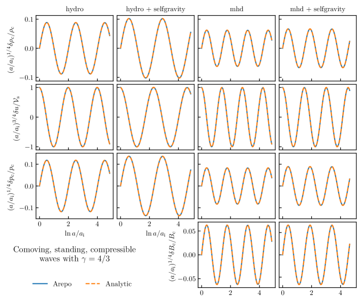
Figure 2: Comparison between analytic theory and arepo simulations of a compressible, standing perturbation in a gas with adiabatic index $\gamma=4/3$ residing in an EdS universe (Sections 3.5.1 and 5.2). We show hydrodynamics (first column), hydrodynamics plus self-gravity (second column), MHD (third column) and MHD plus self-gravity (last column). The wave frequency decreases when self-gravity is included and increases when magnetic fields are included. The analytic solutions are given by equations (56) and (57) (Fourier amplitudes) or equations (81) and (82) (real space assuming $\delta\rho_{\mathrm{c}}(a_{\mathrm{i}})=0$).

We solve equation (49) for the special case $\gamma=4/3$. In this case, the equation reduces to

$$\frac{\partial^{2}{}}{\partial{a}^{2}}\frac{\delta\rho_{\mathrm{c}}}{\rho_{\mathrm{c}}}+\frac{3}{2a}\frac{\partial{}}{\partial{a}}\frac{\delta\rho_{\mathrm{c}}}{\rho_{\mathrm{c}}}+\frac{\sigma^{2}}{a^{2}}\frac{\delta\rho_{\mathrm{c}}}{\rho_{\mathrm{c}}}=0\ ,$$ (51)

where we have defined

$$\sigma\equiv\sqrt{\Omega_{\mathrm{s}}^{2}+\Omega_{\mathrm{A}}^{2}-\Omega_{\mathrm{g}}^{2}}=\frac{k}{H_{0}}\sqrt{\mathcal{V}_{\mathrm{s}}^{2}+\mathcal{V}_{\mathrm{A}}^{2}-\mathcal{V}_{\mathrm{g}}^{2}}\ .$$ (52)

As for the comoving Alfvén wave, this ODE is an Euler equation. Solving the indicial equation, we find the solution for the density to be

$$\frac{\delta\rho_{\mathrm{c}}}{\rho_{\mathrm{c}}}=a^{-1/4}\left(c_{1}\mathrm{e}^{\mathrm{i}\kappa\ln a}+c_{2}\mathrm{e}^{-\mathrm{i}\kappa\ln a}\right)\ ,$$ (53)

where

$$\kappa=\sqrt{\sigma^{2}-\frac{1}{16}}\ .$$ (54)

The velocity solution is given by

$$\frac{\delta u}{\mathcal{V}_{\mathrm{s}}}=\frac{\mathrm{i}\sqrt{a}}{\Omega_{\mathrm{s}}}\frac{\partial{}}{\partial{a}}\frac{\delta\rho_{\mathrm{c}}}{\rho_{\mathrm{c}}}\ ,$$ (55)

and the solution for initial condition $\delta\rho_{\mathrm{c}}(a_{\mathrm{i}})/\rho_{\mathrm{c}}=A_{\rho}$ and $\delta u(a_{\mathrm{i}})/\mathcal{V}_{\mathrm{s}}=A_{u}$ is

$$\frac{\delta\rho_{\mathrm{c}}}{\rho_{\mathrm{c}}}=\left(\frac{a}{a_{\mathrm{i}}}\right)^{-1/4}\left[A_{\rho}\cos(\psi)+\frac{A_{\rho}-4\mathrm{i}\Omega_{\mathrm{s}}\sqrt{a_{\mathrm{i}}}A_{u}}{4\kappa}\sin(\psi)\right]\ ,$$ (56)

$$\frac{\delta u}{\mathcal{V}_{\mathrm{s}}}=\left(\frac{a}{a_{\mathrm{i}}}\right)^{-3/4}\left[A_{u}\cos\left(\psi\right)-\left(\frac{A_{u}}{4\kappa}+\mathrm{i}A_{\rho}\frac{1+16\kappa^{2}}{16\sqrt{a_{\mathrm{i}}}\kappa\Omega_{\mathrm{s}}}\right)\sin\left(\psi\right)\right]\ ,$$ (57)

where $\psi=\kappa\ln\left({a}/{a_{\mathrm{i}}}\right)$. This solution simplifies considerably when $A_{\rho}=0$. We show examples of the solution with this initial condition in Fig. 2. The solutions all have $\Omega_{\mathrm{s}}=\pi$ with $\Omega_{\mathrm{A}}=\pi$ when magnetic fields are included and $\Omega_{\mathrm{g}}=\pi/2$ when self-gravity is included.

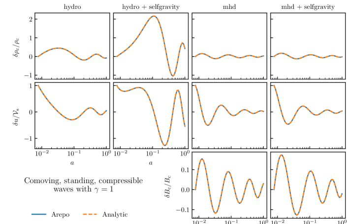
Figure 3: Comparison between analytic theory and arepo simulation of a compressible, standing perturbation in an isothermal gas with adiabatic index $\gamma=1$ residing in an EdS universe (Sections 3.5.2 and 5.2.2). The hydrodynamic simulation with self-gravity has a larger amplitude than the others because the wave is gravitationally unstable for $a<1/16$ (see equation 50). The magnetic field in the MHD simulation with self-gravity is strong enough to fully prevent gravitational instability but the wave frequency is still decreased compared to the MHD simulation without self-gravity. The analytic solutions are given by equations (65) and (67) (Fourier amplitudes). The hydrodynamic solution without self-gravity can be written in simple form, see equations (86) and (87) (real space assuming $\delta\rho_{\mathrm{c}}(a_{\mathrm{i}})=0$).

This solution for a comoving magnetosonic wave modified by self-gravity in EdS cosmology has several interesting features. We observe from equation (52) that $\sigma^{2}$ can be either positive or negative, depending on the relative strengths of $\Omega_{\mathrm{s}}$, $\Omega_{\mathrm{A}}$ and $\Omega_{\mathrm{g}}$ (or alternatively, $\mathcal{V}_{\mathrm{s}}$, $\mathcal{V}_{\mathrm{A}}$ and $\mathcal{V}_{\mathrm{g}}$).

The solution consists of traveling (or oscillating) waves whose amplitude decay with power law rates ($a^{-1/4}$ for $\delta\rho_{\mathrm{c}}/\rho_{\mathrm{c}}$ and $a^{-3/4}$ for $\delta u/\mathcal{V}_{\mathrm{s}}$) when $\sigma^{2}>1/16$. As in fixed frame MHD, the magnetic field increases the frequency of the wave while self-gravity decreases the frequency of the wave (see equations 52 and 54). The oscillatory feature of the solution disappears when $0<\sigma^{2}<1/16$. In this case the perturbations instead suffer a power law decay in a manner similar to the weak magnetic field solution found for comoving Alfvén waves.

Finally, $\kappa$ becomes imaginary with $|\kappa|>1/4$ when $\sigma^{2}<0$ and the amplitude of the perturbation therefore grows in time. The underlying physical mechanism is gravitational instability of the wave which is seen from equation (52) to occur when $\mathcal{V}_{\mathrm{g}}^{2}>\mathcal{V}_{\mathrm{s}}^{2}+\mathcal{V}_{\mathrm{A}}^{2}$. This criterion agrees with equation (50) which was heuristically derived.

The compressible waves with $\gamma=4/3$ are dispersive. We show this by calculating the wave frequency by taking the time derivative of $\psi$, this yields

$$\dot{\psi}=k\left(\mathcal{V}_{\mathrm{s}}^{2}+\mathcal{V}_{\mathrm{A}}^{2}-\mathcal{V}_{\mathrm{g}}^{2}\right)^{1/2}a^{-3/2}\sqrt{1-\frac{1}{16\sigma^{2}}}\ .$$ (58)

Since $\sigma$ depends on $k$ and enters the square root in equation (58) the waves with $\gamma=4/3$ are dispersive, in particular for waves close to the damping scale. A comparison between equation (58) and the fixed frame wave frequency (see e.g. Pringle & King 2014)

$$\omega=k^{\prime}\left(c_{\mathrm{s}}^{2}+\varv_{\mathrm{A}}^{2}-\varv_{\mathrm{g}}^{2}\right)^{1/2}=ka^{-3/2}\left(\mathcal{V}_{\mathrm{s}}^{2}+\mathcal{V}_{\mathrm{A}}^{2}-\mathcal{V}_{\mathrm{g}}^{2}\right)^{1/2}\ ,$$ (59)

reveals that the $a^{-3/2}$ dependence given in equation (58) is as expected from the decrease in wavenumber, $k^{\prime}=k/a$, and the $a^{-1/2}$ decay of $c_{\mathrm{s}}$, $\varv_{\mathrm{A}}$ and $\varv_{\mathrm{g}}$ that occurs during cosmic expansion when $\gamma=4/3$.

As for the Alfvén wave, we are also interested in obtaining the eigenmode in order to be able to initialize traveling waves. We use our knowledge of the solution (equations 56 and 57) to write equations (46) and (47) as the eigenvalue problem

$$\left(\begin{matrix}-\mathrm{i}/4-\kappa&-\Omega_{\mathrm{s}}\\ -\sigma^{2}/\Omega_{\mathrm{s}}&\mathrm{i}/4-\kappa\end{matrix}\right)\left(\begin{matrix}\delta\rho_{\mathrm{c}}/\rho_{\mathrm{c}}a^{1/4}\\ \delta u/\mathcal{V}_{\mathrm{s}}a^{3/4}\end{matrix}\right)=\left(\begin{matrix}0\\ 0\end{matrix}\right)\ .$$ (60)

Solving this eigenvalue problem, we find that the eigenvalues $\pm\kappa$ have eigenmodes given by

$$\frac{\delta\rho_{\mathrm{c}}}{\rho_{\mathrm{c}}} = -C\Omega_{\mathrm{s}}\frac{\pm 4\kappa-\mathrm{i}}{4\sigma^{2}}a^{-1/4}\mathrm{e}^{\pm\mathrm{i}\kappa\ln a}\ ,$$ (61)

$$\frac{\delta u}{\mathcal{V}_{\mathrm{s}}} = Ca^{-3/4}\mathrm{e}^{\pm\mathrm{i}\kappa\ln a}\ ,$$ (62)

where $C$ is the mode amplitude.

3.5.2 Magnetosonic waves with self-gravity and $\gamma\neq 4/3$

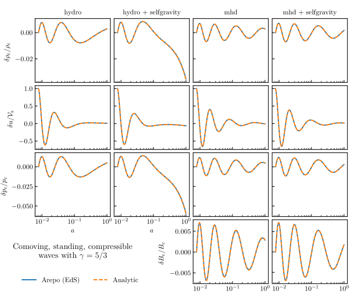
Figure 4: Comparison between analytic theory and arepo simulation of a compressible, standing perturbation in a gas with adiabatic index $\gamma=5/3$ residing in an EdS universe (Sections 3.5.2 and 5.2.3). We show hydrodynamics (first column), hydrodynamics plus self-gravity (second column), MHD (third column) and MHD plus self-gravity (last column). The hydrodynamic simulation with self-gravity is seen to go gravitationally unstable towards the end of the simulation. This is in agreement with equation (50) which for our parameters predicts that this should occur when $a>4/25$. The magnetic field in the MHD simulation with self-gravity is strong enough to prevent the gravitational instability. The general analytic solutions are given by equations (65) and (67) (Fourier amplitudes) but the hydrodynamic solution without self-gravity can be written in a much simpler form, see equations (89) and (90) (real space assuming $\delta\rho_{\mathrm{c}}(a_{\mathrm{i}})=0$).

By comparing equation (49) with equation 6.80 in §104 in Bowman (1958) we find that it is a transformed Bessel equation which has a known analytic solution (see details in Appendix C.3). By introducing two additional parameters,

$$s\equiv\frac{4-3\gamma}{2}\ ,$$ (63)

$$\nu\equiv\frac{\sqrt{1-16{\left(\Omega_{\mathrm{A}}^{2}-\Omega_{\mathrm{g}}^{2}\right)}}}{4|s|}\ ,$$ (64)

the solution for $\delta\rho_{\mathrm{c}}/\rho_{\mathrm{c}}$ can be written as

$$\frac{\delta\rho_{\mathrm{c}}}{\rho_{\mathrm{c}}}=c_{1}\mathcal{F}(a)+c_{2}\mathcal{G}(a)\ ,$$ (65)

where $c_{1}$ and $c_{2}$ are integrations constants and the functions $\mathcal{F}(a)$ and $\mathcal{G}(a)$ are given by

$$\mathcal{F}(a)=a^{-1/4}J_{\nu}\left(z\right)\ ,\quad\mathcal{G}(a)=a^{-1/4}Y_{\nu}\left(z\right)\ .$$ (66)

Here $J_{\nu}\left(z\right)$ and $Y_{\nu}\left(z\right)$ are Bessel functions of the first and second kind, respectively, and we have introduced $z=\Omega_{\mathrm{s}}a^{s}/|s|$ as a short-hand for their argument.

The solution for $\delta u$ is found by differentiation using equation (47) and is given by

$$\frac{\delta u}{\mathcal{V}_{\mathrm{s}}}=i\frac{\sqrt{a}}{\Omega_{\mathrm{s}}}\Big{[}c_{1}\mathcal{F}^{\prime}(a)+c_{2}\mathcal{G}^{\prime}(a)\Big{]}\ .$$ (67)

The integration constants, $c_{1}$ and $c_{2}$, are determined from the initial conditions, $A_{\rho}=\delta\rho_{\mathrm{c}}(a_{\mathrm{i}})/\rho_{\mathrm{c}}$ and $A_{u}=\delta u(a_{\mathrm{i}})/\mathcal{V}_{\mathrm{s}}$. The details are given in Appendix C.3 with the results for $c_{1}$ and $c_{2}$ in equations (140) and (141).

The solution simplifies considerably when initial conditions with $A_{\rho}=0$ are considered. In this case, the solution is given by

$$\frac{\delta\rho_{\mathrm{c}}}{\rho_{\mathrm{c}}} = \,\,\,\,A_{u}\mathrm{i}\Omega_{\mathrm{s}}\frac{\pi a_{\mathrm{i}}}{2s}\Big{[}\mathcal{G}(a_{\mathrm{i}})\mathcal{F}(a)-\mathcal{F}(a_{\mathrm{i}})\mathcal{G}(a)\Big{]}\ ,$$ (68)

$$\frac{\delta u}{\mathcal{V}_{\mathrm{s}}} = -A_{u}\sqrt{a}\frac{\pi a_{\mathrm{i}}}{2s}\Big{[}\mathcal{G}(a_{\mathrm{i}})\mathcal{F}^{\prime}(a)-\mathcal{F}(a_{\mathrm{i}})\mathcal{G}^{\prime}(a)\Big{]}\ .$$ (69)

The effects of magnetic field and self-gravity are contained in the $\nu$ parameter given in equation (64). This parameter is real if the magnetic field is weak but it becomes imaginary if the magnetic field strength is strong enough to make the radicand negative, i.e., if $\Omega_{\mathrm{A}}^{2}>1/16+\Omega_{\mathrm{g}}^{2}$. As described in Matyshev & Fohtung (2009), Bessel functions of imaginary order appear less frequently in scientific applications than the more standard Bessel functions of real order. Perhaps for this reason, not all Bessel function libraries allow for evaluation of non-real order functions (e.g. the scipy special function library only supports real order at the time of writing). We note that both mathematica and the Python library mpmath (Johansson et al., 2021) are able to evaluate Bessel functions for imaginary $\nu$. We make our Python implementation of equations (65) and (67) available online in order to make the analytic solution more easily accessible.

We can find the analytic solution for comoving soundwaves by ignoring the effects of magnetic field and self-gravity. The resulting expressions are given solely in terms of elementary functions. We are particularly interested in isothermal ($\gamma=1$) and adiabatic ($\gamma=5/3$) sound waves (sections 5.2.2 and 5.2.3). Both these cases have $|s|=1/2$ which gives $\nu=1/2$ when $\Omega_{\mathrm{A}}=\Omega_{\mathrm{g}}=0$. The analytic solutions given by equations (68) and (69) then simplify dramatically as the Bessel functions reduce as follows (Abramowitz & Stegun, 1972)

$$\frac{J_{1/2}(z)}{\sin(z)}=-\frac{Y_{1/2}(z)}{\cos(z)}=\sqrt{\frac{2}{\pi z}}\ .$$ (70)

The analytic solutions used to compare with hydrodynamic simulations in Sections 5.2.2 and 5.2.3 were obtained by applying this reduction to equations (68) and (69).

4 Numeric solutions

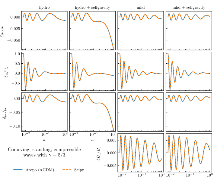
Figure 5: Comparison between a numeric solution of the linearized equations (using scipy) and an arepo simulation of a compressible, standing perturbation in a gas with adiabatic index $\gamma=5/3$ residing in a $\Lambda$CDM universe (Sections 4 and 5.2.4). A comparison with Fig. 4 reveals that one difference between $\Lambda$CDM and EdS is that the wave performs more oscillations in $\Lambda$CDM than in EdS. The explanation for this is probably (at least partially) that the cosmic time duration of the $\Lambda$CDM simulation is roughly 40 percent longer than the EdS simulation.

The analytic wave solutions presented in Sections 3.4 and 3.5 are restricted to cosmologies where the evolution of the scale factor takes the simple EdS form. Here we treat the more general $\Lambda$CDM model by solving the first order ODE systems numerically.

In terms of the parameter $\delta w=a\delta u$ the linearized Alfvén wave equations are

$$\frac{\partial{}}{\partial{a}}\frac{\delta B_{\mathrm{c}}}{B_{\mathrm{c}}}=\frac{\mathrm{i}k}{a^{2}\dot{a}}\delta w\ ,$$ (71)

$$\frac{\partial{\delta w}}{\partial{a}}=\frac{\mathrm{i}k\mathcal{V}_{\mathrm{A}}^{2}}{a\dot{a}}\frac{\delta B_{\mathrm{c}}}{B_{\mathrm{c}}}\ ,$$ (72)

while the compressible, linearized equations are

$$\frac{\partial{}}{\partial{a}}\frac{\delta\rho_{\mathrm{c}}}{\rho_{\mathrm{c}}} =-\frac{\mathrm{i}k}{a^{2}\dot{a}}\delta w\ ,$$ (73)

$$\frac{\partial{\delta w}}{\partial{a}} =-\frac{\mathrm{i}k}{\dot{a}}\left(\frac{\mathcal{V}_{\mathrm{s}}^{2}}{a^{3(\gamma-1)}}+\frac{\mathcal{V}_{\mathrm{A}}^{2}-\mathcal{V}_{\mathrm{g}}^{2}}{a}\right)\frac{\delta\rho_{\mathrm{c}}}{\rho_{\mathrm{c}}}\ .$$ (74)

In these equations $\dot{a}$ is given by the Friedmann equation (equation 92). We use Scipy’s ODE solver to solve these initial value problems.

We show solutions for compressible waves with $\delta\rho_{\mathrm{c}}(a_{\mathrm{i}})=0$ with $\Omega_{\mathrm{m}}=0.3$ and $\Omega_{\Lambda}=0.7$ in Fig. 5. The scipy solution for the Alfvén wave in $\Lambda$CDM is not presented in the paper but we make our script available online.

5 Example code testing with Arepo

We use the analytic solutions derived in Sections 3.4 and 3.5 to compare with results obtained from simulations performed with arepo (Springel, 2010; Weinberger et al., 2020). We use the MHD implementation described in Pakmor et al. (2011); Pakmor & Springel (2013) and the improvements described in Pakmor et al. (2016).

The simulations are performed on a domain of length $L$. The waves are initialized with dimensionless amplitude $A_{u}=10^{-6}$ and wavenumber $kL=2\pi$ at redshift $127$ (corresponding to $a_{\mathrm{i}}=1/128$) unless otherwise specified. The standing wave simulations are initialized by perturbing the velocity only with $\delta u(a_{\mathrm{i}})=A_{u}\mathcal{V}_{\mathrm{A}}\cos(kx)$ for Alfvén waves and $\delta u(a_{\mathrm{i}})=A_{u}\mathcal{V}_{\mathrm{s}}\cos(kx)$ for compressible waves. The traveling waves are initialized using the analytic solutions at $a=a_{\mathrm{i}}$. The amplitudes shown in the figures have been divided by the value of $A_{u}$ such that the velocity amplitude appears as 1 at $a=a_{\mathrm{i}}$.

Most of our simulations are performed in 1D on a static, equidistant grid. In order to better test the Voronoi grid in arepo, the convergence studies presented in Figures 6, 7 and 9 are however performed in 2D. These 2D simulations have size $L_{x}\times L_{y}$ with $N_{x}\times N_{y}$ mesh generating points where we set $N_{y}=4$ and $L_{y}=L_{x}N_{y}/N_{x}$. The Voronoi generating points are given by a regular Cartesian, uniform grid where every second row has been displaced by $0.45L_{x}/N_{x}$. This procedure creates an elongated, hexagonal grid with roughly uniform resolution along each direction.

5.0.1 Periodic self-gravity in 1D

arepo normally employs a sophisticated, so-called TreePM gravity solver which combines an oct-tree algorithm for short-range forces with a particle-mesh (PM) algorithm for long range forces (Springel 2005, 2010, see Weinberger et al. 2020 for a recent discussion of the arepo implementation). The implementation is however multi-dimensional and cannot be used for 1D simulations. While it would be possible to perform the wave tests in 3D, we decided to instead implement a simple 1D Poisson solver. In this implementation, we discretize equation (11) using finite differences on an equidistant grid and obtain the potential by solving the resulting matrix equation (using GMRES from the GSL library, see Gough 2009). We then use centered finite differences to find the gravitational acceleration. The implementation is limited to equidistant grids but suffices for our purposes.

5.0.2 Cosmological source term when $\gamma\neq 1$ and $\gamma\neq 5/3$

The comoving version of arepo normally assumes either $\gamma=1$ or $5/3$. The tests with $\gamma=4/3$ in Section 5.2.1 therefore required implementing an extra source term MHD in the energy equation. We provide the details in Appendix B with the extra term in the energy equation given in equation (127).

5.1 Comoving Alfvén waves

5.1.1 Standing Alfvén waves

The analytic solution for a linearly polarized Alfvén wave is derived in Section 3.4 with the result for the Fourier mode amplitudes given by equations (28) and (29). When the initial perturbation is such that $\delta B_{\mathrm{c}}(a_{\mathrm{i}})=0$, the solution in real space can be written

$$\frac{\delta B_{\mathrm{c}}(x,a)}{B_{\mathrm{c}}} = -A_{u}\left(\frac{a}{a_{\mathrm{i}}}\right)^{-1/4}\frac{\sqrt{a_{\mathrm{i}}}\Omega_{\mathrm{A}}}{\kappa}\sin(\psi)\sin\left(kx\right),\,\quad$$ (75)

$$\frac{\delta u(x,a)}{\mathcal{V}_{\mathrm{A}}} = A_{u}\left(\frac{a}{a_{\mathrm{i}}}\right)^{-3/4}\left(\cos\left(\psi\right)-\frac{\sin\left(\psi\right)}{4\kappa}\right)\cos\left(kx\right)\ ,$$ (76)

where $\Omega_{\mathrm{A}}$, $\kappa$ and $\psi$ are defined in equations (17), (26) and (30), respectively.

We use this solution to initialize a simulation with $\Omega_{\mathrm{A}}=\pi$ and show the amplitude evolution of the wave in Fig. 1. The arepo solution is seen to closely follow the theoretical expectation.

A more detailed understanding of the frequency and amplitude error found using arepo can be found by performing a series of simulations at various spatial resolutions. We perform such a study in 2D where we expect second order convergence from the space and time discretization in arepo (Pakmor et al., 2016). We also use a stronger magnetic field, $\Omega_{\mathrm{A}}=2\pi$ in order to have many oscillations occurring between $a_{\mathrm{i}}=1/128$ and $a=1$.

The result of this convergence study is shown in Fig. 6. In the left panel we show $\delta B_{\mathrm{c}}/B_{\mathrm{c}}$ multiplied with $a^{1/4}$ and $\delta u/\mathcal{V}_{\mathrm{A}}$ multiplied with $a^{3/4}$ as a function of $\ln a/a_{\mathrm{i}}$. The advantage of plotting the solution this way is that it makes the correct solution appear as simple sinusoidal functions. This makes it easy to visually distinguish the numeric decay of the wave from the physical one. In addition to this visual assessment, we also fit the arepo data with functions of the form

$$y(x)=C\sin\left(\kappa_{\mathrm{num}}x+D\right)\mathrm{e}^{-\Gamma_{\mathrm{num}}x/2}\ ,$$ (77)

where $x=\ln(a/a_{\mathrm{i}})$ and $y=\delta B_{\mathrm{c}}a^{1/4}$ or $y=\delta u\,a^{3/4}$ are values obtained from the simulations. Here $C$, $D$, $\kappa_{\mathrm{num}}$ and $\Gamma_{\mathrm{num}}$ are fitting parameters. As evident in the left panel of Fig. 6 such fits provide an excellent match to the simulation data. The error in the frequency is shown in the top right panel of Fig. 6 (here $\kappa_{\mathrm{num}}$ is the frequency found in the simulation data and $\kappa$ is the theoretical expectation). The numeric decay rate, $\Gamma_{\mathrm{num}}/2$, is shown in the bottom right panel of Fig. 6. The frequency error is seen to converge at second order while the numeric decay rate converges at third order.

The time steps in arepo are performed in units of $\ln a$. The erroneous power law damping can therefore be understood as a constant amplification factor applied at each time step equidistantly spaced in $\ln a$ (see e.g. chapter 2 in Durran 2010 for the definition of the amplification factor). Alternatively, this damping can be understood as arising from a redshift dependent numerical viscosity coefficient. In order to make this interpretation, we amend our analytic solution for Alfvén waves to include Navier-Stokes viscosity. The derivation is given in Appendix C.4 with the analytic solution given in Equations (153) and (154). The solution shows that the numerical decay given by $\Gamma_{\mathrm{num}}/2$ can be described as arising due to a numerical viscosity coefficient $\eta_{\mathrm{num}}=\eta_{\mathrm{num},0}\,a^{-5/2}$ where $\eta_{\mathrm{num},0}$ is the numerical viscosity coefficient at $z=0$. The relation $\Gamma_{\mathrm{num}}=\eta_{\mathrm{num},0}\,k^{2}/(\rho_{\mathrm{c}}H_{0})$ allows us to find the numerical viscosity coefficient from the fits shown in Fig. 6. We find

$$\eta_{\mathrm{num}}\approx 0.072\times\frac{\rho_{\mathrm{c}}H_{0}}{k^{2}}\left(\frac{N_{x}}{16}\right)^{-2.99}a^{-5/2}\ ,$$ (78)

which shows how the numerical viscosity, $\eta_{\mathrm{num}}$, depends on scale factor and resolution. While this numerical viscosity picture describes the amplitude damping it does not fully explain the simulation results. Indeed, while a physical viscosity would decrease the wave frequency (see Appendix C.4), low resolution arepo solutions are instead seen to display a higher frequency than the analytic solution. This means that arepo’s update procedure is accelerating rather than decelerating (see e.g. chapter 2 in Durran 2010 for definitions of this terminology).

5.1.2 Traveling Alfvén waves

We use the eigenmode for a traveling Alfvén wave derived in Section 3.4 to initialize arepo simulations. Equations (33) and (34) are Fourier amplitudes so we need to construct the solution in real space. A wave traveling to the right (left) is simply found by multiplying the minus (plus) solution by $\mathrm{e}^{\mathrm{i}kx}$ and taking the real part. We find it useful to write the solution using the amplitude $A_{u}=Ca_{\mathrm{i}}^{-3/4}\mathrm{e}^{\pm\mathrm{i}\kappa\ln a_{\mathrm{i}}}$. The wave traveling to the right is then given by

$$\frac{\delta B_{\mathrm{c}}}{B_{\mathrm{c}}} = A_{u}\frac{\sqrt{a_{\mathrm{i}}}}{4\Omega_{\mathrm{A}}}\left(\frac{a}{a_{\mathrm{i}}}\right)^{-1/4}\Big{[}\sin\left(kx-\psi\right)-4\kappa\cos\left(kx-\psi\right)\Big{]}\ ,\quad\quad$$ (79)

$$\frac{\delta u}{\mathcal{V}_{\mathrm{A}}} = A_{u}\left(\frac{a}{a_{\mathrm{i}}}\right)^{-3/4}\cos\left(kx-\psi\right)\ ,$$ (80)

where $A_{u}$ is the dimensionless velocity amplitude. We take $\Omega_{\mathrm{A}}=\pi$ and perform 2D simulations with $N_{x}=8$, 16, 32 and 64. The simulations are initialized such that exactly $n$ periods elapse between $a_{\mathrm{i}}$ and $a=1$. This is done by setting $a_{\mathrm{i}}=\mathrm{e}^{-2n\pi/\kappa}$ where $n$ is the number of times the wave traverses the box. We choose $n=2$ such that $a_{\mathrm{i}}\approx 0.01808$ for this test.

The traveling wave makes it easy to distinguish between frequency and amplitude errors, as evident in the left column of Fig. 7 where we show the wave profiles at $a=1$. For instance, we observe that the waves are traveling too fast in the low resolution arepo simulations (i.e. $\kappa_{\mathrm{num}}>\kappa$). The (absolute, maximum) difference between theory and simulation converges at second order, as shown on the right in Fig. 7.

5.1.3 Alfvén waves with a deliberately introduced bug in arepo

Many types of programming errors in the $a$-factors will lead to nonsensical results or perhaps even premature termination of a simulation (if infinities or nans develop). Here we illustrate that some errors in $a$-factors can lead to subtle effects that are not so easily found by the code developer. This exercise is done to show that sensible looking simulations that do not crash are not necessarily bug-free.

We use for our example the MHD flux calculation as developed by Pakmor & Springel (2013) and described in their section 2.2. In their algorithm the magnetic field is scaled as $\bm{B}^{\prime}_{\mathrm{c}}=\bm{B}_{\mathrm{c}}/\sqrt{a}$ (their step ii), a Riemann solver is used to calculate the flux, $\bm{F}^{\prime}_{B}$ (their step iii), and finally the scaling of the magnetic field is reverted by transforming the flux: $\bm{F}_{B}=\bm{F}^{\prime}_{B}\times\sqrt{a}$ (their step iv).

We stress that this implementation works in arepo. Let us, however, imagine that something went wrong in step iv such that either $\bm{F}_{B}=\bm{F}^{\prime}_{B}$ (the flux was never rescaled, we will call this hypothetical bug "Bug 1") or $\bm{F}_{B}=\bm{F}^{\prime}_{B}\times a$ (the flux was rescaled by the wrong $a$-factor, we will call this hypothetical bug "Bug 2").

We intentionally introduce these two types of bugs in the arepo source code and perform standing, Alfvén wave simulations using the same parameters and field strength as in Fig. 1, i.e., $\Omega_{\mathrm{A}}=\pi$. The two types of bugs lead to the wrong frequency and amplitude evolution of the Alfvén wave. This is evident in Fig. 8 where we compare with the original (and correct) implementation. While problems are immediately discovered using the Alfvén wave test, it is less obvious how these bugs would manifest themselves in a so-called "full physics" cosmological simulation. One merit of the Alfvén wave test is thus that it catches even subtle errors.

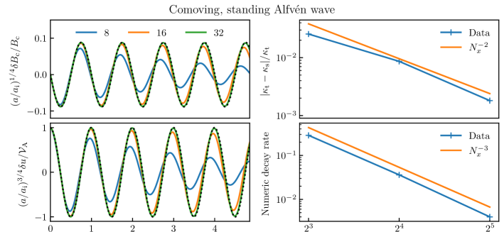
Figure 6: Convergence test of a standing Alfvén wave in EdS cosmology (Section 3.4 and 5.1.1). Left panel: the amplitudes of $\delta B_{\mathrm{c}}$ (top) and $\delta u$ (bottom) scaled with appropriate powers of $a$ such that the solutions appear sinusoidal when plotted versus $\ln a/a_{\mathrm{i}}$. The decay in amplitude is therefore due to numerical dissipation only. The analytic solution is shown with solid black lines while fits to equation (77) are shown with dotted black lines. The labels indicate the number of cells in the $x$-direction. With $N_{x}=32$ the arepo simulation data coincides visually with the analytic solution while $N_{x}=16$ ($N_{x}=8$) has (significant) amplitude and frequency error. Right panel: Convergence of the frequency (top) and numerical decay rate (bottom).

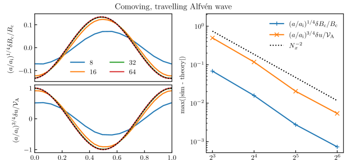
Figure 7: Convergence test of a traveling Alfvén wave in EdS cosmology (Section 3.4 and 5.1.2). The wave is initialized at $a_{\mathrm{i}}=\mathrm{e}^{-2\pi n/\kappa}$ with $n=2$ such that it has traveled twice across the simulation domain by $a=1$. Left panel: the arepo simulation data for $\delta B_{\mathrm{c}}$ (top) and $\delta u$ (bottom) is shown as a function of $x$ at $a=1$. The amplitudes are appropriately scaled with powers of $a/a_{\mathrm{i}}$ such that the initial condition (shown with a dashed black line) coincides with the analytic solution at $a=1$ despite the wave decaying in amplitude while it travels. The extra decay found in the lower resolution simulations is therefore due to numerical dissipation. The analytic solution is given by equations (33) and (34) (Fourier amplitudes) or equations (79) and (80) (in real space). Right panel: The maximum of the absolute difference between arepo simulation and analytic solution at $a=1$ converges at second order.

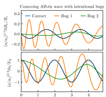
Figure 8: Alfvén wave in EdS cosmology with intentionally introduced bugs in the MHD flux calculation (Section 3.4 and 5.1.3). Bug 1 (2) has an extra factor of $a^{-1/2}$ ($a^{1/2}$) in the flux. This leads to a too high (Bug 1) or too low (Bug 2) frequency as compared to the correct result. The analytic theory is shown with a dashed black line. The example is meant to illustrate how an error in the MHD flux calculation can be detected.

5.2 Comoving compressible waves

5.2.1 Waves with $\gamma=4/3$

The baryonic gas in cosmological simulations is normally assumed to obey an adiabatic equation of state with $\gamma=5/3$ (e.g. Weinberger et al. 2020). The value chosen in the following test, $\gamma=4/3$, has the curious feature that the thermal, magnetic and gravitational forces decay at the same rate. This value of $\gamma$ describes a gas with a relativistic equation of state. While a relativistic component is expected in the form of cosmic rays accelerated at e.g. structure formation shocks (e.g. Pfrommer et al. 2006), the equations of ideal MHD that we use here do not correctly include all the relevant terms (see e.g. Pfrommer et al. 2017 for the equations for fluid cosmic rays coupled to thermal gas in a comoving frame). Nevertheless, we argue that the following examples are useful because their analytic solutions are given in terms of simple, elementary functions. This is an advantage compared to the $\gamma=1$ or $\gamma=5/3$ solutions presented in Section 3.5.2 whose evaluation require Bessel functions of imaginary order. In addition, it is possible to set up both standing and traveling compressible waves for $\gamma=4/3$. This is only possible because the wave eigenmode is known (see Section 3.5.1).

Standing waves

We take $\Omega_{\mathrm{s}}=\pi$ with $\Omega_{\mathrm{A}}=\pi$ for MHD simulations and $\Omega_{\mathrm{g}}=\pi/2$ for simulations with self-gravity (with $\Omega_{\mathrm{A}}=0$ when MHD is turned off and $\Omega_{\mathrm{g}}=0$ when self-gravity is turned off). The general analytic solution for the Fourier amplitudes for this problem are given by equations (56) and (57) in Section 3.5.1. When $\delta\rho_{\mathrm{c}}(a_{\mathrm{i}})=0$, the analytic solution in real space can be written

$$\frac{\delta\rho_{\mathrm{c}}}{\rho_{\mathrm{c}}}=A_{u}\left(\frac{a}{a_{\mathrm{i}}}\right)^{-1/4}\frac{\Omega_{\mathrm{s}}\sqrt{a_{\mathrm{i}}}}{\kappa}\sin(\psi)\sin(kx)\ ,\quad\quad$$ (81)

$$\frac{\delta u}{\mathcal{V}_{\mathrm{s}}}=A_{u}\left(\frac{a}{a_{\mathrm{i}}}\right)^{-3/4}\left(\cos\left(\psi\right)-\frac{\sin\left(\psi\right)}{4\kappa}\right)\cos(kx)\ ,$$ (82)

where $\kappa$ is defined in equation (54) and $\psi=\kappa\ln\left({a}/{a_{\mathrm{i}}}\right)$. The comparison between theory and simulation is presented in Fig. 2 where we find excellent agreement. We note that the solutions have been scaled and plotted versus $\ln a/a_{\mathrm{i}}$ such that they appear as sinusoidal functions with constant amplitude (in the same way as we did for the Alfvén wave in Fig. 6).

Consistent with equation (54), the magnetic field is seen to increase the frequency of the wave while self-gravity decreases the frequency. The same qualitative behaviour is seen in standard, non-comoving ideal MHD (e.g. Pringle & King 2014). The physical mechanism is that the magnetic pressure acts as a restoring force in unison with the thermal pressure while self-gravity acts in the opposite direction and therefore decreases the frequency. In addition to the changes in frequency, self-gravity also slightly increases the amplitude of the density perturbation relative to simulations without self-gravity (this is clearly visible in the hydrodynamic simulations) while the magnetic field slightly decreases the amplitude.

Traveling waves

Here we initialize an arepo simulation with waves traveling to the right. The analytic solution was derived in Section 3.5.1 and can be written in real space as

$$\frac{\delta\rho_{\mathrm{c}}}{\rho_{\mathrm{c}}} = A_{u}\frac{\Omega_{\mathrm{s}}\sqrt{a_{\mathrm{i}}}}{4\sigma^{2}}\left(\frac{a}{a_{\mathrm{i}}}\right)^{-1/4}\left[4\kappa\cos\left(kx-\psi\right)-\sin\left(kx-\psi\right)\right]\ ,\quad\ \,$$ (83)

$$\frac{\delta u}{\mathcal{V}_{\mathrm{s}}} = A_{u}\left(\frac{a}{a_{\mathrm{i}}}\right)^{-3/4}\cos\left(kx-\psi\right)\ ,$$ (84)

where $\sigma$ was defined in equation (52). We set $\Omega_{\mathrm{s}}=\Omega_{\mathrm{A}}=\pi$ and $\Omega_{\mathrm{g}}=0$ and start the simulation at $a_{\mathrm{i}}=\mathrm{e}^{-2n\pi/\kappa}$ where $\kappa$ is defined in equation (54) and $n$ is the number of times the wave travels through the box. We set $n=3$ such that $a_{\mathrm{i}}\approx 0.01427$ for this test.

We perform 2D simulations and vary $N_{x}$ in powers of 2 between 8 and 64. We show the results in Fig. 9 with the wave profiles on the left and the convergence results on the right. As for the traveling Alfvén wave, we find second order convergence of the (absolute, maximum) difference between theory and simulation.

5.2.2 Isothermal waves

We next consider waves with an isothermal equation of state (i.e. $\gamma=1$). The interesting feature for an isothermal equation of state is that the overall strength of the thermal restoring force of the wave does not decay as a function of redshift. This means that it is possible to set up a simulation which is initially dominated by magnetic and/or gravitational forces and then transitions to be dominated by thermal forces. By carefully choosing the parameters ($\Omega_{\mathrm{s}}$, $\Omega_{\mathrm{A}}$ and $\Omega_{\mathrm{g}}$), it is possible to have the time period where gravity dominates long enough that a strong modification is seen (relative to simulations without self-gravity) but short enough that the wave remains firmly in the linear regime. We have found the parameters $\Omega_{\mathrm{s}}=2\pi$ with $\Omega_{\mathrm{A}}=\pi$ when MHD is turned on and $\Omega_{\mathrm{g}}=\pi/2$ when self-gravity is turned on to result in this behaviour.

We show the results of simulations with these parameters in Fig. 3. The hydrodynamic solution with self-gravity is shown in the second column of Fig. 3. This solution has a decreased frequency and a very large density amplitude compared to the hydrodynamic solution without self-gravity (its larger by a factor of almost five). The extra growth in density amplitude is seen to occur at early times. This is in good agreement with equation (50) which predicts that gravity dominates for $a<1/16$. The magnetic field in the MHD plus self-gravity simulation dominates gravity at all times (since $\Omega_{\mathrm{A}}>\Omega_{\mathrm{g}}$ and the forces decay at the same rate). There is therefore only a slight increase in the density amplitude relative to the MHD simulation without self-gravity (compare the third and fourth columns in Fig. 3).

The relevant theory for these simulations was derived in Section 3.5 with the Fourier amplitudes given by equations (68) and (69) in Section 3.5.2. The solution can be written in a much simpler form for the hydrodynamic problem without self-gravity. In this case, we find for $\gamma=1$ that the analytic solution for a standing wave in real space is

$$\frac{\delta\rho_{\mathrm{c}}(x,\,a)}{\rho_{\mathrm{c}}} = A_{u}\sqrt{\frac{a_{\mathrm{i}}}{a}}\sin\left(\phi\right)\sin\left(kx\right)\ ,$$ (86)

$$\frac{\delta u(x,\,a)}{\mathcal{V}_{\mathrm{s}}} = A_{u}\left[\sqrt{\frac{a_{\mathrm{i}}}{a}}\cos\left(\phi\right)-\frac{\sqrt{a_{\mathrm{i}}}}{2\Omega_{\mathrm{s}}a}\sin\left(\phi\right)\right]\cos\left(kx\right)\ ,\quad$$ (87)

where $\phi=2\Omega_{\mathrm{s}}\left(\sqrt{a}-\sqrt{a_{\mathrm{i}}}\right)$. As evident in Fig. 3, the simulations agree very well with the evolutions predicted by the analytic theory.

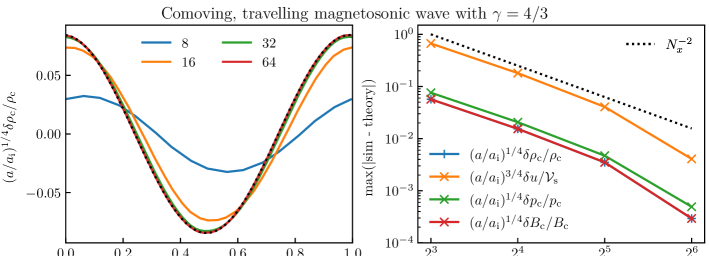
Figure 9: Same as Fig. 7 but here for a traveling magnetosonic wave with $\gamma=4/3$ and $\Omega_{\mathrm{s}}=\Omega_{\mathrm{A}}=\pi$ which has traveled three times through the box (Sections 3.5.1 and 5.2). The analytic solutions are given by equations (61) and (62) (Fourier amplitudes) and equations (83) and (84) (in real space).

5.2.3 Adiabatic waves in EdS

We proceed by studying adiabatic waves by setting $\gamma=5/3$. This is the value used in almost all cosmological MHD simulations and is consequently a very relevant test case. In addition, $\gamma=5/3$ has the interesting feature that the thermal force decays faster than the gravitational and magnetic forces. This means that it is possible to set up a wave which is initially gravitationally stable but transitions to gravitational instability once the thermal pressure drops below a critical value. We use equation (50) to set up the parameters in precisely this way, i.e., the hydrodynamic simulation with self-gravity goes unstable near the end of simulation. We choose the value of $\Omega_{\mathrm{A}}$ such that the MHD simulation with self-gravity is stable at all times. Choosing the parameters this way gives a qualitative difference between the hydrodynamic and MHD tests including self-gravity (rather than just a quantitative change in frequency and amplitude). Given this motivation, we take $\Omega_{\mathrm{s}}=\pi/5$ with $\Omega_{\mathrm{A}}=\pi$ for MHD simulations and $\Omega_{\mathrm{g}}=\pi/2$ for simulations with self-gravity.

A comparison between arepo simulations and analytic theory is shown in Fig. 4. We note the excellent agreement between the two and the onset of gravitational instability in the hydrodynamic simulation with self-gravity (second column in Fig. 4) as well as the absence of gravitational instability in the MHD plus self-gravity simulation (fourth column).

The analytic solutions used for the comparison are given by equations (65) and (67) in Section 3.5.2. The hydrodynamic wave without magnetic fields and self-gravity can be written in a much simpler form. For $\gamma=5/3$, the solution with $\delta\rho_{\mathrm{c}}(a_{\mathrm{i}})=0$ becomes

$$\frac{\delta\rho_{\mathrm{c}}(x,\,a)}{\rho_{\mathrm{c}}} = A_{u}a_{\mathrm{i}}\sin\left(\varphi\right)\sin\left(kx\right)\ ,$$ (89)

$$\frac{\delta u(x,\,a)}{\mathcal{V}_{\mathrm{s}}} = A_{u}\frac{a_{\mathrm{i}}}{a}\cos\left(\varphi\right)\cos\left(kx\right)\ ,\quad$$ (90)

where

$$\varphi=2\Omega_{\mathrm{s}}\left(\frac{1}{\sqrt{a_{\mathrm{i}}}}-\frac{1}{\sqrt{a}}\right)\ .$$ (91)

5.2.4 Adiabatic waves in $\Lambda\mathrm{CDM}$

We perform arepo simulations of adiabatic waves in $\Lambda$CDM cosmology. We set $\Omega_{\mathrm{m},0}=0.3$ and $\Omega_{\Lambda,0}=0.7$ in equation (1) and keep all other parameters as in the preceding section where we used EdS cosmology. It is important to note that we do not include any dark matter particles in the simulation. That is, the test only includes dark matter as a uniform background which influences the evolution of $a$ via the Friedmann equation (equation 1).

We do not have an analytic solution for $\Lambda$CDM and instead compare the arepo simulations with the numeric solution described in section 4. This comparison between arepo simulation and scipy solution is shown in Fig. 5. It it interesting to compare the $\Lambda$CDM results (Fig. 5) with those found for EdS (Fig. 4). The most notable difference between waves in the two cosmologies is that the waves oscillate more times in $\Lambda$CDM than in EdS. The main reason for this is likely that the cosmic time duration between $a_{\mathrm{i}}=1/128$ and $a_{\mathrm{i}}=1$ is roughly 40 percent longer in $\Lambda$CDM than it is in EdS.

6 Discussion

With the rapid increase in the complexity of codes for computational astrophysics, the code development is increasingly becoming a continued and collaborative effort. In order to avoid introduction of errors (so-called bugs) and to ensure that a given code version is fit for production runs, developers are using version control systems (primarily git version control, see e.g. Chacon & Straub 2014) and adapting software engineering practices such as automated testing. This practice allows for continuous integration of new features into the main code version (with git by making a pull-request from a development branch into the main branch).

However, an essential ingredient necessary for building confidence in this process is that the test suite covers all the intended use cases. Since comoving MHD codes are generally tested by using test problems developed for standard MHD codes (by setting $a=1$ and $\dot{a}=0$), we argue in this paper that this criterion for a successful testing framework is often not fulfilled. This does not necessarily mean that published results relying on cosmological MHD simulations are wrong but rather that the underlying code base could be vulnerable to the introduction of errors in the source code (a regression).

The purpose of the present paper is to remedy this issue by introducing new tests specifically designed to help find programming errors related to $a$ and $\dot{a}$. These new tests consist of analytic solutions for Alfvén and magnetosonic waves in EdS cosmology (derived in Section 3) and numeric solutions for those waves in $\Lambda$CDM (described in Section 4). We have used these hydromagnetic solutions to compare with the MHD code arepo in Section 5. Reassuringly, we have in all cases found excellent agreement with arepo.

Many of the mistakes possible when introducing scale factors in a code will lead to obviously meaningless results or premature termination of the code. However, it is also possible to have implementation mistakes that cause more subtle errors. We make this point explicit by intentionally introducing bugs in arepo in Section 5.1.3. As seen in Fig. 8, the intentionally wrong simulations are able to proceed until $a=1$ without the introduction of obviously wrong values in the solution. However, comparison with the analytic solution immediately reveals that there is a problem.

Subtle errors are also more likely to be introduced when additional physical effects are included in a code base. As an example, assume that the viscosity term in comoving coordinates scales as $a^{n}$. If the programmer by mistake instead implements viscosity with a term proportional to $a^{n+1}$ then this will not lead to a crash. Instead, the included effective viscosity will simply be less than the physically expected value. This type of error is difficult to find without proper tests (Berlok et al, in prep.).

In addition to error finding, it is also possible that our tests can help distinguish the advantages and disadvantages of various methods for numerically solving the comoving MHD equations (i.e. by studying wave amplitude and frequency errors at a given numerical resolution as in Figs. 6, 7 and 9).

For the reasons outlined above, we are of the view that these tests, specifically designed for comoving MHD, will be an useful addition to automated testing frameworks of comoving MHD codes.

As a final remark, we note that other fluid dynamics tests could be fruitfully extended to the comoving coordinate system as well. While analytic solutions might not always be possible, high fidelity numeric solutions will be. One particular interesting but simple type of system that could be investigated is the shock tube problem in comoving coordinates.

Data availability

Python code for evaluating the analytic solutions presented in Section 3 and for re-computing the numeric solutions presented in Section 4 can be downloaded at https://github.com/tberlok/comoving_mhd_waves. A public version of the arepo code has been made available by the main developers (Weinberger et al., 2020) and can be downloaded at https://gitlab.mpcdf.mpg.de/vrs/arepo. We will share our setup for initializing and analyzing arepo simulations upon request.

Appendix A Comoving MHD tests currently in use in the literature

We provide a short description of the tests normally used to test implementations of comoving hydrodynamics and/or MHD.

A common test case for hydrodynamics in comoving coordinates is the so-called Zel’dovich pancake problem which is based on the analytic results by Zel’Dovich (1970). This test combines self-gravity and a hydrodynamic fluid and follows gravitational collapse in an EdS cosmology. The Zel’dovich pancake problem has been used in many papers including Cen (1992); Ryu et al. (1993); Bryan et al. (1995); Trac & Pen (2004); Bryan et al. (2014) and Springel (2010). It has been also been extended to MHD in Collins et al. (2010) and Hopkins & Raives (2016). The magnetic field evolution in these simulations is compared with reference simulations which have been performed with other codes or the same code at higher resolution.

Another common test is to consider a uniform universe in which there are no peculiar motions (see e.g. Collins et al. 2010 and Ruszkowski et al. 2011). This reduces the comoving MHD equations to a system of ordinary differential equations which can be analytically integrated. This type of test is useful for verifying the implementation of comoving source terms but it has the limitation that it does not verify the calculation of gradients and fluxes.

The Santa-Barbara cluster consists of a set of fixed initial conditions for a $10^{15}M_{\odot}$ galaxy cluster (Frenk et al., 1999). The diagnostics for this test are global properties, projection images and radial profiles of various gas quantities (e.g. gas density, pressure and temperature and dark matter density). The Santa-Barbara cluster is an already non-trivial problem and obtaining the physically correct radial profiles can be difficult (see Springel 2010 for a discussion). The Santa-Barbara cluster was introduced in 1999 at a time when most cosmological simulations did not include magnetic fields. In recent years it has been extended to MHD in Miniati & Martin (2011); Hopkins & Raives (2016) and Hopkins (2016) but a code-comparison project including MHD has not yet been done. Simulations performed by Vazza et al. (2018) have found that very high spatial resolution is required to obtain a converged magnetic field in non-radiative MHD simulations of a galaxy clusters. We argue that this makes the Santa-Barbara cluster unfeasible for frequent regression testing of comoving MHD.

Finally, most code papers contain example applications of their codes, e.g., simulations of individual galaxies or galaxy clusters. These tests are useful for stress-testing, as codes will sometimes crash in realistic applications even though they perform well on all the idealized test problems. The disadvantage of using tests that are so close to the target science is that there is rarely a universally agreed-upon correct solution (an example is the MHD version of the Santa-Barbara cluster discussed above).

We have here only described the tests commonly used for comoving MHD. It it therefore worth mentioning that cosmological codes typically also test their gravity implementations against an extensive list of standard tests (see e.g. Springel et al. 2021; Dakin et al. 2021; Angulo & Hahn 2022).

Appendix B Transformation of MHD equations to comoving coordinates

B.1 Friedmann equations

The evolution of the scale factor, $a$, in a flat universe depends on the cosmological parameters for the total matter density (baryonic plus dark matter), $\Omega_{\mathrm{m},0}$, radiation, $\Omega_{\mathrm{r},0}$, and dark energy, $\Omega_{\Lambda,0}$. This dependence is given by the Friedmann equation (e.g. Cimatti et al. 2019; Angulo & Hahn 2022)

$$\left(\frac{\dot{a}}{a}\right)^{2}=\frac{8\pi G}{3}\bar{\rho}_{\mathrm{tot}}\ ,$$ (92)

where

$$\bar{\rho}_{\mathrm{tot}}=\left(\frac{\Omega_{\mathrm{r},0}}{a^{4}}+\frac{\Omega_{\mathrm{m},0}}{a^{3}}+\Omega_{\Lambda,0}\right)\rho_{\mathrm{crit},0}\ ,$$ (93)

is the mean of the total density, $\rho_{\mathrm{crit},0}=3H_{0}^{2}/(8\pi G)$ is the critical density, and $H_{0}$ is the Hubble parameter at $z=0$. Equations (92) and (93) can be combined into equation (1) used in the main body of the paper.

B.2 The coordinate transformation

We briefly review how to transform from the fixed $\bm{r}$ coordinates to the comoving $\bm{x}$ coordinates. We consider a general function of $\bm{r}$ and $t$, say $f(\bm{r},\,t)$. From the point of point of view of the $\bm{r}$ coordinate system, the convective time-derivative is

$$\frac{df}{dt}=\left(\frac{\partial{f}}{\partial t}\right)_{\bm{r}}+\left(\dot{\bm{r}}\mbox{\boldmath{$\cdot$}}\nabla_{\bm{r}}\right)f\ ,$$ (94)

where the partial time-derivative is at fixed position $\bm{r}$. Given the relation, $\bm{r}=a\bm{x}$, $\dot{\bm{r}}$ can be written out as

$$\dot{\bm{r}}=\bm{\varv}=\dot{a}{\bm{x}}+a\dot{\bm{x}}\ =\dot{a}{\bm{x}}+\bm{u}\ ,$$ (95)

where we have defined the peculiar, physical velocity, $\bm{u}\equiv a\dot{\bm{x}}$. The convective derivative can thus also be written

$$\frac{df}{dt}=\left(\frac{\partial{f}}{\partial t}\right)_{\bm{r}}+\dot{a}\left({\bm{x}}\mbox{\boldmath{$\cdot$}}\nabla_{\bm{r}}\right)f+\left(\bm{u}\mbox{\boldmath{$\cdot$}}\nabla_{\bm{r}}\right)f\ .$$ (96)

From the point of view of the comoving coordinate system, the convective derivative is

$$\frac{df}{dt}=\left(\frac{\partial{f}}{\partial t}\right)_{\bm{x}}+\left(\dot{\bm{x}}\mbox{\boldmath{$\cdot$}}\nabla_{\bm{x}}\right)f=\left(\frac{\partial{f}}{\partial t}\right)_{\bm{x}}+\frac{1}{a}\left(\bm{u}\mbox{\boldmath{$\cdot$}}\nabla_{\bm{x}}\right)f\ ,$$ (97)

where the partial time-derivative is at fixed $\bm{x}$.

We now use that the convective derivative has a unique value which does not depend on the coordinate system. Noting that the gradient operators are simply related

$$\nabla_{\bm{r}}f=\frac{1}{a}\nabla_{\bm{x}}f\ ,$$ (98)

we can therefore equate equations (96) and (97) to find a relation between the partial time-derivatives in the two coordinate systems. This yields

$$\left(\frac{\partial{f}}{\partial t}\right)_{\bm{r}}=\left(\frac{\partial{f}}{\partial t}\right)_{\bm{x}}-\frac{\dot{a}}{a}\left({\bm{x}}\mbox{\boldmath{$\cdot$}}\nabla_{\bm{x}}\right)f\ .$$ (99)

B.3 Continuity equation

With $\rho=\rho_{\mathrm{c}}a^{-3}$ and $\bm{\varv}=\dot{a}{\bm{x}}+\bm{u}$ equation (2) becomes

$$\frac{d\ln\rho_{\mathrm{c}}}{dt}-3\frac{d\ln a}{dt}=-\frac{\dot{a}}{a}\nabla_{\bm{x}}\mbox{\boldmath{$\cdot$}}\bm{x}-\frac{1}{a}\nabla_{\bm{x}}\mbox{\boldmath{$\cdot$}}\bm{u}\ .$$ (100)

Since $\nabla_{\bm{x}}\mbox{\boldmath{$\cdot$}}\bm{x}=3$, the terms involving $\dot{a}$ cancel out and we obtain equation (7).

B.4 Momentum equation

The momentum equation, equation (3), is transformed by substituting $p=a^{-3}p_{\mathrm{c}}$, $\rho=a^{-3}\rho_{\mathrm{c}}$, $\bm{B}=a^{-2}\bm{B}_{\mathrm{c}}$, replacing $\nabla_{\bm{r}}$ with $\nabla_{\bm{x}}/a$ and finally multiplying through by $a^{4}$. This yields

$$\rho_{\mathrm{c}}a\left[\frac{d(\dot{a}\bm{x})}{dt}+\frac{d\bm{u}}{dt}\right]=-\nabla_{\bm{x}}p_{\mathrm{c}}-\frac{1}{a}\nabla_{\bm{x}}\mbox{\boldmath{$\cdot$}}\left(\frac{B_{\mathrm{c}}^{2}}{2}\mathbf{1}-\bm{B}_{\mathrm{c}}\bm{B}_{\mathrm{c}}\right)-\rho_{\mathrm{c}}\nabla_{\bm{x}}\Phi\ ,$$ (101)

where

$$\frac{d(\dot{a}\bm{x})}{dt}=\left(\frac{\partial{(\dot{a}\bm{x})}}{\partial t}\right)_{\bm{x}}+\frac{1}{a}\left(\bm{u}\mbox{\boldmath{$\cdot$}}\nabla_{\bm{x}}\right)\left(\dot{a}\bm{x}\right)=\ddot{a}\bm{x}+\frac{\dot{a}}{a}\bm{u}\ .$$ (102)

We conclude that the momentum equation can be written

$$\rho_{\mathrm{c}}\frac{d\bm{u}}{dt}=-\frac{1}{a}\nabla_{\bm{x}}p_{\mathrm{tot,c}}-\rho_{\mathrm{c}}\frac{\dot{a}}{a}\bm{u}-\rho_{\mathrm{c}}\ddot{a}\bm{x}+\frac{1}{a^{2}}\nabla_{\bm{x}}\mbox{\boldmath{$\cdot$}}\left(\bm{B}_{\mathrm{c}}\bm{B}_{\mathrm{c}}\right)-\rho_{\mathrm{c}}\frac{1}{a}\nabla_{\bm{x}}\Phi\ ,$$ (103)

where we have introduced the total pressure $p_{\mathrm{tot,c}}=p_{\mathrm{c}}+B_{\mathrm{c}}^{2}/(2a)$.

The gravitational potential, $\Phi$, fulfills the Poisson equation

$$\nabla_{\bm{r}}^{2}\Phi=4\pi G\rho_{\mathrm{tot}}\ ,$$ (104)

where $\rho_{\mathrm{tot}}$ is the total density which enters the first Friedmann equation (equation 92, Angulo & Hahn 2022). Thus depending on the cosmological model employed, $\rho_{\mathrm{tot}}$ can include contributions from both baryonic and dark matter as well as radiation and the cosmological constant.

It is conventional to split $\Phi$ into two contributions, $\Phi=\Phi_{0}+\delta\Phi$, by splitting the density into two contributions, $\rho_{\mathrm{tot}}=\bar{\rho}_{\mathrm{tot}}+\delta\rho_{\mathrm{tot}}$ where $\bar{\rho}_{\mathrm{tot}}$ is the mean density and $\delta\rho_{\mathrm{tot}}$ is the local deviation, i.e., $\delta\rho_{\mathrm{tot}}=\rho_{\mathrm{tot}}-\bar{\rho}_{\mathrm{tot}}$. This can be done without loss of generality and $|\delta\rho_{\mathrm{tot}}/\bar{\rho}_{\mathrm{tot}}|$ does not have to be small. The splitting yields two separate Poisson equations, i.e.,

$$\nabla_{\bm{r}}^{2}\Phi_{0}=4\pi G\bar{\rho}_{\mathrm{tot}}\ ,$$ (105)

and

$$\nabla_{\bm{r}}^{2}\delta\Phi=4\pi G\,\delta\rho_{\mathrm{tot}}=4\pi G\left(\rho_{\mathrm{tot}}-\bar{\rho}_{\mathrm{tot}}\right)\ .$$ (106)

Equation 105 can be analytically integrated because $\bar{\rho}_{\mathrm{tot}}$ is constant in space. The solution is $\Phi_{0}=2\pi G\bar{\rho}_{\mathrm{tot}}r^{2}/3$. Since $\bar{\rho}_{\mathrm{tot}}$ is the density in a homogeneous universe, it is given in terms of the second Friedmann equation (see e.g. Carroll 2004)

$$\frac{\ddot{a}}{a}=-\frac{4\pi G}{3}\bar{\rho}_{\mathrm{tot}}\ .$$ (107)

Using this expression for the total density it is concluded that

$$\Phi_{0}=-\frac{1}{2}\frac{\ddot{a}}{a}r^{2}=-\frac{1}{2}a\ddot{a}x^{2}$$ (108)

where $r=ax$ was used in the second step. This agrees with equation 7.7 in Peebles (1980). The potential has the property that

$$\ddot{a}\bm{x}=-\frac{1}{a}\nabla_{\bm{x}}\Phi_{0}\ ,$$ (109)

which can be seen to eliminate the $\rho_{\mathrm{c}}\ddot{a}\bm{x}$ source term in the momentum equation (103). That is, the fictitious force that arises from moving into a non-inertial reference frame is canceled by the background gravitational force. Substituting the potential $\Phi=\Phi_{0}+\delta\Phi$ into the momentum equation, we thus find

$$\rho_{\mathrm{c}}\frac{d\bm{u}}{dt}=-\frac{1}{a}\nabla_{\bm{x}}p_{\mathrm{tot,c}}-\rho_{\mathrm{c}}\frac{\dot{a}}{a}\bm{u}+\frac{1}{a^{2}}\nabla_{\bm{x}}\mbox{\boldmath{$\cdot$}}\left(\bm{B}_{\mathrm{c}}\bm{B}_{\mathrm{c}}\right)-\rho_{\mathrm{c}}\frac{1}{a}\nabla_{\bm{x}}\delta\Phi\ ,$$ (110)

Finally, the remaining Poisson equation for $\delta\Phi$ is converted to comoving coordinates by defining the comoving total density, $\rho_{\mathrm{c,tot}}=\rho_{\mathrm{tot}}a^{3}$. This gives

$$\nabla_{\bm{x}}^{2}\delta\Phi=\frac{4\pi G}{a}\left(\rho_{\mathrm{c,tot}}-\bar{\rho}_{\mathrm{c,tot}}\right)\ .$$ (111)

Sometimes the Poisson equation is further rewritten as (see e.g. Weinberger et al. 2020)

$$\nabla_{\bm{x}}^{2}\delta\Phi_{\mathrm{c}}=4\pi G\left(\rho_{\mathrm{c,tot}}-\bar{\rho}_{\mathrm{c,tot}}\right)\ .$$ (112)

by defining the comoving potential as $\delta\Phi_{\mathrm{c}}=a\delta\Phi$ which is then related to the full potential by

$$\delta\Phi_{\mathrm{c}}=a\Phi+\frac{1}{2}a^{2}\ddot{a}x^{2}\ .$$ (113)

B.5 Induction equation

Converting the time and space derivatives to the comoving coordinates, equation (4) becomes

$$\left(\frac{\partial{\bm{B}}}{\partial t}\right)_{\bm{x}}=\frac{\dot{a}}{a}\left(\bm{x}\mbox{\boldmath{$\cdot$}}\nabla_{\bm{x}}\right)\bm{B}+\frac{1}{a}\nabla_{\bm{x}}\times\left(\bm{\varv}\times\bm{B}\right)\ .$$ (114)

Substituting variables with comoving variables, we obtain

$$\left(\frac{\partial{\bm{B}_{\mathrm{c}}}}{\partial t}\right)_{\bm{x}}-\frac{1}{a}\nabla_{\bm{x}}\times\left(\bm{u}\times\bm{B}_{\mathrm{c}}\right)=\\ \frac{\dot{a}}{a}\left[2\bm{B}_{\mathrm{c}}+\left(\bm{x}\mbox{\boldmath{$\cdot$}}\nabla_{\bm{x}}\right)\bm{B}_{\mathrm{c}}+\nabla_{\bm{x}}\times\left(\bm{x}\times\bm{B}_{\mathrm{c}}\right)\right]\ ,$$ (115)

Using a standard vector identity (see e.g. Spruit 2013) we find

$$\nabla_{\bm{x}}\times\left(\bm{x}\times\bm{B}_{\mathrm{c}}\right)=-2\bm{B}_{\mathrm{c}}-\left(\bm{x}\mbox{\boldmath{$\cdot$}}\nabla_{\bm{x}}\right)\bm{B}_{\mathrm{c}}$$ (116)

which shows that the RHS of equation (115) is zero. The comoving induction equation is therefore given by equation (9).

B.6 Internal energy equation

We transform equation (6) by defining the comoving internal energy as $\varepsilon_{\mathrm{c}}=\varepsilon a^{3}$. We substitute the comoving variables and obtain

$$\frac{d\ln\varepsilon_{\mathrm{c}}}{dt}-3\frac{d\ln a}{dt}=-\gamma\frac{1}{a}\nabla_{\bm{x}}\mbox{\boldmath{$\cdot$}}\left(\dot{a}\bm{x}+\bm{u}\right)\ .$$ (117)

which, given that $\nabla_{\bm{x}}\mbox{\boldmath{$\cdot$}}\bm{x}=3$, reduces to equation (10).

B.7 Conservative form and total energy equation

Cosmological MHD codes solve the comoving MHD equations in form which is as close to a set of conservation laws as possible. While equations (7)–(11) are adequate for the analytic work presented here, we have found it useful to connect our derivation to the existing literature.

We therefore briefly explain how to convert to the form given in Pakmor & Springel (2013). The equations presented here, however, include gravity and do not assume $\gamma=5/3$. The derivation helped us understand how the extra energy source term that arises when $\gamma\neq 5/3$ should be implemented in the arepo code.

The continuity equation, equation (7), can also be written as

$$\left(\frac{\partial{\rho_{\mathrm{c}}}}{\partial t}\right)_{\bm{x}}+\frac{1}{a}\nabla_{\bm{x}}\mbox{\boldmath{$\cdot$}}\left(\rho\bm{u}\right)=0\ .$$ (118)

Equation (110) can be transformed into an equation for $\rho_{\mathrm{c}}\bm{u}$ by writing out the convective derivative and using the mass continuity equation. The momentum equation then becomes

$$\left(\frac{\partial{\rho_{\mathrm{c}}\bm{u}}}{\partial t}\right)_{\bm{x}}+\frac{1}{a}\nabla_{\bm{x}}\mbox{\boldmath{$\cdot$}}\left[\rho_{\mathrm{c}}\bm{u}\bm{u}+p_{\mathrm{tot,c}}\mbox{\boldmath{$1$}}-\frac{\bm{B}_{\mathrm{c}}\bm{B}_{\mathrm{c}}}{a}\right]=-\rho_{\mathrm{c}}\frac{\dot{a}}{a}\bm{u}-\rho_{\mathrm{c}}\frac{1}{a}\nabla_{\bm{x}}\delta\Phi\ .$$ (119)

The total energy equation requires additional derivations. As in Pakmor & Springel (2013), we define the total energy as

$$E_{\mathrm{c}}=\varepsilon_{\mathrm{c}}+\frac{1}{2}\rho_{\mathrm{c}}u^{2}+\frac{B_{\mathrm{c}}^{2}}{2a}\ .$$ (120)

The internal energy equation in conservative form becomes

$$\left(\frac{\partial{\varepsilon_{\mathrm{c}}}}{\partial t}\right)_{\bm{x}}+\frac{1}{a}\nabla_{\bm{x}}\mbox{\boldmath{$\cdot$}}\left(\varepsilon_{\mathrm{c}}\bm{u}\right)=-p_{\mathrm{c}}\frac{1}{a}\nabla_{\bm{x}}\mbox{\boldmath{$\cdot$}}\bm{u}-3\frac{\dot{a}}{a}\left(\gamma-1\right)\varepsilon_{\mathrm{c}}\ .$$ (121)

The kinetic energy equation is found by dotting equation (119) with $\bm{u}$. After some manipulation one finds

$$\left(\frac{\partial}{\partial t}\frac{\rho_{\mathrm{c}}u^{2}}{2}\right)_{\bm{x}}+\frac{1}{a}\nabla_{\bm{x}}\mbox{\boldmath{$\cdot$}}\left[\frac{\rho_{\mathrm{c}}u^{2}}{2}\bm{u}+p_{\mathrm{tot,c}}\bm{u}-\frac{\bm{B}_{\mathrm{c}}\left(\bm{u}\mbox{\boldmath{$\cdot$}}\bm{B}_{\mathrm{c}}\right)}{a}\right]=\\ +\left(p_{\mathrm{c}}+\frac{B_{\mathrm{c}}^{2}}{2a}\right)\frac{1}{a}\nabla_{\bm{x}}\mbox{\boldmath{$\cdot$}}\bm{u}-\frac{1}{a^{2}}\bm{B}_{\mathrm{c}}\bm{B}_{\mathrm{c}}\mbox{\boldmath{$:$}}\nabla_{\bm{x}}\bm{u}-\rho_{\mathrm{c}}\frac{1}{a}\left(\bm{u}\mbox{\boldmath{$\cdot$}}\nabla_{\bm{x}}\right)\delta\Phi-\rho_{\mathrm{c}}\frac{\dot{a}}{a}u^{2}\ ,$$ (122)

where the $\mathbf{:}$ notation is short-hand for the trace of a matrix product (in index notation $\bm{A}\bm{B}\mathbf{:}\bm{C}\bm{D}=\sum_{i}\sum_{j}A_{i}B_{j}C_{i}D_{j}$).

The magnetic energy equation is found by dotting equation (9) with $\bm{B}_{\mathrm{c}}$. One finds

$$\left(\frac{\partial}{\partial t}\frac{B_{\mathrm{c}}^{2}}{2}\right)_{\bm{x}}+\frac{1}{a}\nabla_{\bm{x}}\mbox{\boldmath{$\cdot$}}\left(\frac{B_{\mathrm{c}}^{2}}{2}\bm{u}\right)=-\frac{1}{a}\left[\frac{B_{\mathrm{c}}^{2}}{2}\nabla_{\bm{x}}\mbox{\boldmath{$\cdot$}}\bm{u}-\bm{B}_{\mathrm{c}}\bm{B}_{\mathrm{c}}\mbox{\boldmath{$:$}}\nabla_{\bm{x}}\bm{u}\right]\ ,$$ (123)

which is straightforward to convert to an evolution equation for $B_{\mathrm{c}}^{2}/2a$. We find

$$\left(\frac{\partial}{\partial t}\frac{B_{\mathrm{c}}^{2}}{2a}\right)_{\bm{x}}+\frac{1}{a}\nabla_{\bm{x}}\mbox{\boldmath{$\cdot$}}\left(\frac{B_{\mathrm{c}}^{2}}{2a}\bm{u}\right)=-\frac{B_{\mathrm{c}}^{2}}{2a}\frac{1}{a}\nabla_{\bm{x}}\mbox{\boldmath{$\cdot$}}\bm{u}+\frac{1}{a^{2}}\bm{B}_{\mathrm{c}}\bm{B}_{\mathrm{c}}\mbox{\boldmath{$:$}}\nabla_{\bm{x}}\bm{u}-\frac{B_{\mathrm{c}}^{2}}{2a}\frac{\dot{a}}{a}\ .$$ (124)

The evolution equation for $E_{\mathrm{c}}$ is now found by adding up equations (121), (122) and (124). Most of the RHS terms cancel out as they correspond to transfer of energy between thermal, kinetic and magnetic energy densities (as in standard MHD). The equation for the comoving energy becomes

$$\left(\frac{\partial{E_{\mathrm{c}}}}{\partial t}\right)_{\bm{x}}+\frac{1}{a}\nabla_{\bm{x}}\mbox{\boldmath{$\cdot$}}\left[\left(E_{\mathrm{c}}+p_{\mathrm{tot,c}}\right)\bm{u}-\frac{\bm{B}_{\mathrm{c}}\left(\bm{u}\mbox{\boldmath{$\cdot$}}\bm{B}_{\mathrm{c}}\right)}{a}\right]=\\ -\rho_{\mathrm{c}}\frac{1}{a}\left(\bm{u}\mbox{\boldmath{$\cdot$}}\nabla_{\bm{x}}\right)\delta\Phi-\left[3\left(\gamma-1\right)\varepsilon_{\mathrm{c}}+\rho_{\mathrm{c}}u^{2}+\frac{B_{\mathrm{c}}^{2}}{2a}\right]\frac{\dot{a}}{a}\ .$$ (125)

B.8 Conservative form with fewer source terms

The comoving MHD equations found in the literature are equations for $a\rho_{\mathrm{c}}\bm{u}$ and $a^{2}E_{\mathrm{c}}$ rather than simply $\rho_{\mathrm{c}}\bm{u}$ and $E_{\mathrm{c}}$. The reason is that this eliminates some of the cosmological source terms (Pakmor & Springel, 2013).

The conversion of the momentum equation is done by multiplying equation (119) by $a$ and rewriting the time derivative. This yields

$$\left(\frac{\partial{(a\rho_{\mathrm{c}}\bm{u})}}{\partial t}\right)_{\bm{x}}+\nabla_{\bm{x}}\mbox{\boldmath{$\cdot$}}\left[p_{\mathrm{tot,c}}\mathbf{1}+\rho_{\mathrm{c}}\bm{u}\bm{u}-\frac{1}{a}\bm{B}_{\mathrm{c}}\bm{B}_{\mathrm{c}}\right]=-\rho_{\mathrm{c}}\nabla_{\bm{x}}\delta\Phi\ ,$$ (126)

where the only remaining source term is the gravitational one.

It is similarly useful to consider the evolution of $a^{2}E_{\mathrm{c}}$ rather than equation (125). The conversion is done by multiplying by $a^{2}$ and rewriting the time derivative. This gives

$$\left(\frac{\partial{a^{2}E_{\mathrm{c}}}}{\partial t}\right)_{\bm{x}}+a\nabla_{\bm{x}}\mbox{\boldmath{$\cdot$}}\left[\left(E_{\mathrm{c}}+p_{\mathrm{tot,c}}\right)\bm{u}-\frac{\bm{B}_{\mathrm{c}}\left(\bm{u}\mbox{\boldmath{$\cdot$}}\bm{B}_{\mathrm{c}}\right)}{a}\right]=\\ -\rho_{\mathrm{c}}a\left(\bm{u}\mbox{\boldmath{$\cdot$}}\nabla_{\bm{x}}\right)\delta\Phi+\left[\left(5-3\gamma\right)\varepsilon_{\mathrm{c}}+\frac{B_{\mathrm{c}}^{2}}{2a}\right]a\dot{a}\ .$$ (127)

For $\gamma=5/3$ there is only a single (magnetic) cosmological source term in equation (127). When $\gamma\neq 5/3$ there is an additional source term related to the thermal energy. We have implemented this term in arepo in order to perform simulations with $\gamma=4/3$ (i.e. Figures 2 and 9)..

Appendix C Analytic solution details

C.1 Alfvén solution for $\Omega_{\mathrm{A}}=1/4$

Equation (25) is not the solution to equation (24) in the special case $\Omega_{\mathrm{A}}=1/4$ (which gives $\kappa=0$). Instead the solution is

$$\frac{\delta B_{\mathrm{c}}}{B_{\mathrm{c}}}=a^{-1/4}\left(c_{3}+c_{4}\ln a\right)\ ,$$ (128)

where $c_{3}$ and $c_{4}$ are integration constants (Asmar, 2010). The change in solution occurs because the indicial roots of equation (24) are not distinct. This particular value of $\Omega_{\mathrm{A}}$ does not correspond to a wave but we give its solution for completeness. Applying the initial conditions, we find

$$\frac{\delta B_{\mathrm{c}}}{B_{\mathrm{c}}}=\left(\frac{a}{a_{\mathrm{i}}}\right)^{-1/4}\left[A_{B}+\frac{A_{B}+\mathrm{i}\sqrt{a_{\mathrm{i}}}A_{u}}{4}\ln\left(\frac{a}{a_{\mathrm{i}}}\right)\right]\ ,$$ (129)

$$\frac{\delta u}{\mathcal{V}_{\mathrm{A}}}=\left(\frac{a}{a_{\mathrm{i}}}\right)^{-3/4}\left[A_{u}-\frac{A_{u}-\mathrm{i}a_{\mathrm{i}}^{-1/2}A_{B}}{4}\ln\left(\frac{a}{a_{\mathrm{i}}}\right)\right]\ .$$ (130)

C.2 Compressible solution for $\gamma=4/3$ with $\sigma=1/4$

The case $\sigma=1/4$ in equation (51) requires special treatment for the same reason as in Appendix C.1 above. Solving and applying initial conditions, we find that the compressible solution in this case becomes

$$\frac{\delta\rho_{\mathrm{c}}}{\rho_{\mathrm{c}}}=\left(\frac{a}{a_{\mathrm{i}}}\right)^{-1/4}\left[A_{\rho}+\frac{A_{\rho}-4\mathrm{i}\Omega_{\mathrm{s}}\sqrt{a_{\mathrm{i}}}A_{u}}{4}\ln\left(\frac{a}{a_{\mathrm{i}}}\right)\right]\ ,$$ (131)

$$\frac{\delta u}{\mathcal{V}_{\mathrm{s}}}=\left(\frac{a}{a_{\mathrm{i}}}\right)^{-3/4}\left[A_{u}-\left(\frac{A_{u}}{4}+\frac{\mathrm{i}A_{\rho}}{16\sqrt{a_{\mathrm{i}}}\Omega_{\mathrm{s}}}\right)\ln\left(\frac{a}{a_{\mathrm{i}}}\right)\right]\ .$$ (132)

C.3 Comoving magnetosonic wave with self-gravity

This appendix provides additional details on the derivation presented in Section 3.5.2. We compare our equation (49) with equation 6.80 in §104 in Bowman (1958). The latter equation reads

$$\frac{d^{2}y}{dx^{2}}-\frac{2\alpha-1}{x}\frac{dy}{dx}+\left(\beta^{2}\gamma^{\prime 2}x^{2\gamma^{\prime}-2}+\frac{\alpha^{2}-n^{2}\gamma^{\prime 2}}{x^{2}}\right)y=0\ .$$ (133)

Setting $y=\delta\rho_{\mathrm{c}}/\rho_{\mathrm{c}}$ and $x=a$ the comparison immediately reveals that $\alpha=-1/4$ is required in order to match the $dy/dx$ term. Next, we realize that we need $2\gamma^{\prime}-2=2-3\gamma$ in order to have the same power of $x$ in the term proportional to $\beta^{2}$. This leads us to define $s=\gamma^{\prime}\equiv(4-3\gamma)/2$ as in equation (63). We also require $\beta^{2}s^{2}=\Omega_{\mathrm{s}}^{2}$ so that $\beta=\Omega_{\mathrm{s}}/|s|$. Finally we observe that $\alpha^{2}-n^{2}\gamma^{\prime 2}=\Omega_{\mathrm{A}}^{2}-\Omega_{\mathrm{g}}^{2}$ from which we find

$$s^{2}n^{2}=\frac{1}{16}-\left(\Omega_{\mathrm{A}}^{2}-\Omega_{\mathrm{g}}^{2}\right)\ ,$$ (134)

which leads to our definition of $\nu=n$ given in equation (64). According to equation 6.82 in Bowman (1958) the solution to equation 133 valid also for integer $n$ is

$$y=x^{\alpha}\left\{A\,J_{n}\left(\beta x^{\gamma^{\prime}}\right)+B\,Y_{n}\left(\beta x^{\gamma^{\prime}}\right)\right\}\ ,$$ (135)

where $A$ and $B$ are integration constants. The solution to equation (49) is thus given by equation (65) where $\mathcal{F}(a)$ and $\mathcal{G}(a)$ are defined in equation (66).

The integration constants, $c_{1}$ and $c_{2}$, are found by solving two equations for two unknowns: $\delta\rho_{\mathrm{c}}(a_{\mathrm{i}})/\rho_{\mathrm{c}}=c_{1}\mathcal{F}(a_{\mathrm{i}})+c_{2}\mathcal{G}(a_{\mathrm{i}})$ and $\delta\rho_{\mathrm{c}}^{\prime}(a_{\mathrm{i}})/\rho_{\mathrm{c}}=c_{1}\mathcal{F}^{\prime}(a_{\mathrm{i}})+c_{2}\mathcal{G}^{\prime}(a_{\mathrm{i}})$. This yields

$$c_{1}=\frac{\mathcal{G}^{\prime}(a_{\mathrm{i}})}{D(a_{\mathrm{i}})}\frac{\delta\rho_{\mathrm{c}}}{\rho_{\mathrm{c}}}(a_{\mathrm{i}})-\frac{\mathcal{G}(a_{\mathrm{i}})}{D(a_{\mathrm{i}})}\frac{\delta\rho_{\mathrm{c}}^{\prime}}{\rho_{\mathrm{c}}}(a_{\mathrm{i}})\ ,$$ (136)

$$c_{2}=\frac{\mathcal{F}(a_{\mathrm{i}})}{D(a_{\mathrm{i}})}\frac{\delta\rho_{\mathrm{c}}^{\prime}}{\rho_{\mathrm{c}}}(a_{\mathrm{i}})-\frac{\mathcal{F}^{\prime}(a_{\mathrm{i}})}{D(a_{\mathrm{i}})}\frac{\delta\rho_{\mathrm{c}}}{\rho_{\mathrm{c}}}(a_{\mathrm{i}})\ ,$$ (137)

where

$$D(a_{\mathrm{i}})=\mathcal{F}(a_{\mathrm{i}})\mathcal{G}^{\prime}(a_{\mathrm{i}})-\mathcal{F}^{\prime}(a_{\mathrm{i}})\mathcal{G}(a_{\mathrm{i}})=\frac{2s}{\pi a_{\mathrm{i}}^{3/2}}\ .$$ (138)

We simplify these expressions by defining dimensionless amplitudes $A_{u}=\delta u(a_{\mathrm{i}})/\mathcal{V}_{\mathrm{s}}$ and $A_{\rho}=\delta\rho_{\mathrm{c}}(a_{\mathrm{i}})/\rho_{\mathrm{c}}$ and using equation (46) to write

$$\frac{\delta\rho_{\mathrm{c}}^{\prime}}{\rho_{\mathrm{c}}}(a_{\mathrm{i}})=-\frac{\mathrm{i}k}{H_{0}\sqrt{a_{\mathrm{i}}}}\delta u(a_{\mathrm{i}})=-\frac{\mathrm{i}\Omega_{\mathrm{s}}}{\sqrt{a_{\mathrm{i}}}}A_{u}\ .$$ (139)

In terms of these, the integration constants are given by

$$c_{1} = \;\,\,\,\frac{\pi a_{\mathrm{i}}^{3/2}}{2s}\left(\mathcal{G}^{\prime}(a_{\mathrm{i}})A_{\rho}+\mathrm{i}\Omega_{\mathrm{s}}\frac{\mathcal{G}(a_{\mathrm{i}})}{\sqrt{a_{\mathrm{i}}}}A_{u}\right)\ ,$$ (140)

$$c_{2} = -\frac{\pi a_{\mathrm{i}}^{3/2}}{2s}\left(\mathcal{F}^{\prime}(a_{\mathrm{i}})A_{\rho}+\mathrm{i}\Omega_{\mathrm{s}}\frac{\mathcal{F}(a_{\mathrm{i}})}{\sqrt{a_{\mathrm{i}}}}A_{u}\right)\ .$$ (141)

For practical computations we use the following explicit expressions for the derivatives of $\mathcal{F}(a)$ and $\mathcal{G}(a)$:

$$\mathcal{F}^{\prime}(a)=\Omega_{\mathrm{s}}\operatorname{sgn}(s)a^{s-5/4}J^{\prime}_{\nu}\left(z\right)-\frac{1}{4}a^{-5/4}J_{\nu}\left(z\right)\ ,$$ (142)

$$\mathcal{G}^{\prime}(a)=\Omega_{\mathrm{s}}\operatorname{sgn}(s)a^{s-5/4}Y^{\prime}_{\nu}\left(z\right)-\frac{1}{4}a^{-5/4}Y_{\nu}\left(z\right)\ ,$$ (143)

where $\operatorname{sgn}(s)$ is the sign function.

C.4 Alfvén wave including Navier-Stokes viscosity

We provide a derivation of the analytic solution for an Alfvén wave including physical Navier-Stokes viscosity. This solution is used to interpret the numerical dissipation study presented in Fig. 6. The analysis is a generalization of the first part of Section 3.4 in the main text. Here we limit ourselves to standing waves and hence do not provide the expressions for traveling waves with viscosity (mainly due to space restrictions). We also note that it is possible to derive analytic results including viscosity for compressible waves with $\gamma=4/3$. We do not pursue this here but instead refer to Berlok et al, in prep, for such a calculation including Braginskii viscosity.

Navier-Stokes viscosity is included as an additional term on the RHS of equation (3), $-\nabla_{\bm{r}}\mbox{\boldmath{$\cdot$}}\mathbf{\Pi}$, where

$$\mathbf{\Pi}=\eta\left(\nabla_{\bm{r}}\bm{\varv}+\left(\nabla_{\bm{r}}\bm{\varv}\right)^{T}-\frac{2}{3}\mathbf{1}\nabla_{\bm{r}}\mbox{\boldmath{$\cdot$}}\bm{\varv}\right)\ ,$$ (144)

is the viscosity tensor and $\eta$ is the viscosity coefficient. After transforming to comoving coordinates, this leads to an additional term,

$$-a^{2}\eta\nabla_{\bm{x}}\mbox{\boldmath{$\cdot$}}\left(\nabla_{\bm{x}}\bm{u}+\left(\nabla_{\bm{x}}\bm{u}\right)^{T}-\frac{2}{3}\mathbf{1}\nabla_{\bm{x}}\mbox{\boldmath{$\cdot$}}\bm{u}\right)\ ,$$ (145)

on the RHS of equation (8). We will assume that the viscosity coefficient is given by $\eta=\eta_{0}a^{n}$ where $\eta_{0}$ is its value at $z=0$. We further set $n=-5/2$ since this leads to an analytically solvable ODE. We also define a viscosity parameter

$$\Gamma=\frac{\eta_{0}k^{2}}{\rho_{\mathrm{c}}H_{0}}\ ,$$ (146)

which simplifies the following results. The new linearized equations for an Alfvén wave, corresponding to equations (21) and (22), then become

$$\frac{\partial{}}{\partial{a}}\frac{\delta B_{\mathrm{c}}}{B_{\mathrm{c}}}=\frac{\mathrm{i}\Omega_{\mathrm{A}}}{a^{3/2}}\frac{\delta w}{\mathcal{V}_{\mathrm{A}}}\ ,$$ (147)

$$\frac{\partial{}}{\partial{a}}\left(\frac{\delta w}{\mathcal{V}_{\mathrm{A}}}\right)=\frac{\mathrm{i}\Omega_{\mathrm{A}}}{a^{1/2}}\frac{\delta B_{\mathrm{c}}}{B_{\mathrm{c}}}-\frac{\Gamma}{a}\frac{\delta w}{\mathcal{V}_{\mathrm{A}}}\ ,$$ (148)

where $\delta w=a\delta u$. We combine these linearized equations and obtain

$$\frac{\partial^{2}{}}{\partial{a}^{2}}\left(\frac{\delta w}{\mathcal{V}_{\mathrm{A}}}\right)+\frac{1+2\Gamma}{2a}\frac{\partial{}}{\partial{a}}\left(\frac{\delta w}{\mathcal{V}_{\mathrm{A}}}\right)+\frac{\Omega_{\mathrm{A}}^{2}-\Gamma/2}{a^{2}}\frac{\delta w}{\mathcal{V}_{\mathrm{A}}}=0\ ,$$ (149)

which is solved using the usual machinery (Asmar, 2010). We find the solution for $\delta u=\delta w/a$ to be

$$\frac{\delta u}{\mathcal{V}_{\mathrm{A}}}=a^{-3/4-\Gamma/2}\left(c_{1}e^{i\kappa\ln a}+c_{2}e^{-i\kappa\ln a}\right)\ ,$$ (150)

where

$$\kappa\equiv\sqrt{\Omega_{\mathrm{A}}^{2}-\frac{\left(1+2\Gamma\right)^{2}}{16}}\ ,$$ (151)

and $c_{1}$ and $c_{2}$ are integration constants. The solution for $\delta B_{\mathrm{c}}$ is found by integrating equation (147) and is given by

$$\frac{\delta B_{\mathrm{c}}}{B_{\mathrm{c}}}=-\mathrm{i}a^{-1/4-\Gamma/2}\left(c_{3}e^{i\kappa\ln a}+c_{4}e^{-i\kappa\ln a}\right)\ ,$$ (152)

where $c_{3}=4\Omega_{\mathrm{A}}c_{1}/(1+2\Gamma-4\mathrm{i}\kappa)$ and $c_{4}=4\Omega_{\mathrm{A}}c_{2}/(1+2\Gamma+4\mathrm{i}\kappa)$. The solution with $\delta B_{\mathrm{c}}(a_{\mathrm{i}})/B_{\mathrm{c}}=A_{B}$ and $\delta u(a_{\mathrm{i}})/\mathcal{V}_{\mathrm{A}}=A_{u}$ is given by

$$\frac{\delta B_{\mathrm{c}}}{B_{\mathrm{c}}}=\left(\frac{a}{a_{\mathrm{i}}}\right)^{-1/4-\Gamma/2}\Big{[}A_{B}\cos(\psi)+\Big{.}\\ \Big{.}\frac{A_{B}\left(1+2\Gamma\right)+4\mathrm{i}\Omega_{\mathrm{A}}\sqrt{a_{\mathrm{i}}}A_{u}}{4\kappa}\sin(\psi)\Big{]}\ ,$$ (153)

$$\frac{\delta u}{\mathcal{V}_{\mathrm{A}}}=\left(\frac{a}{a_{\mathrm{i}}}\right)^{-3/4-\Gamma/2}\Big{[}A_{u}\cos\left(\psi\right)-\Big{.}\\ \Big{.}\frac{A_{u}\left(1+2\Gamma\right)-4\mathrm{i}\Omega_{\mathrm{A}}a_{\mathrm{i}}^{-1/2}A_{B}}{4\kappa}\sin\left(\psi\right)\Big{]}\ ,$$ (154)

where $\psi=\kappa\ln(a/a_{\mathrm{i}})$ and $\kappa$ is given by equation (151) which includes the viscosity effect. These equations reduce to equations (28) and (29) in the limit of zero viscosity where $\Gamma=0$. Viscosity modifies the wave by increasing the damping (by a factor of $a^{-\Gamma/2}$) and decreasing the frequency (see equation 151). It also changes the criterion for when oscillating waves are possible, i.e., this criterion becomes $\Omega_{\mathrm{A}}>\left(1+2\Gamma\right)/4$ rather than simply $\Omega_{\mathrm{A}}>1/4$. We note that the transition from oscillating waves to pure damping, i.e., $\kappa=0$, requires special treatment (as in Appendix C.1) and has a solution that differs from Equations (153) and (154). We do not pursue this here.

References

- Abramowitz & Stegun (1972) Abramowitz M., Stegun I. A., 1972, Handbook of Mathematical Functions
- Angulo & Hahn (2022) Angulo R. E., Hahn O., 2022, Living Reviews in Computational Astrophysics, 8, 1
- Asmar (2010) Asmar N. H., 2010, Partial differential equations and boundary value problems with fourier series. Pearson Education
- Barkana & Loeb (2001) Barkana R., Loeb A., 2001, Phys. Rep., 349, 125
- Barnes et al. (2018) Barnes D. J., On A. Y. L., Wu K., Kawata D., 2018, MNRAS, 476, 2890
- Berlok et al. (2020) Berlok T., Pakmor R., Pfrommer C., 2020, MNRAS, 491, 2919
- Bowman (1958) Bowman F., 1958, Introduction to Bessel Functions
- Bryan et al. (1995) Bryan G. L., Norman M. L., Stone J. M., Cen R., Ostriker J. P., 1995, Computer Physics Communications, 89, 149
- Bryan et al. (2014) Bryan G. L., et al., 2014, ApJS, 211, 19
- Carroll (2004) Carroll S. M., 2004, Spacetime and geometry. An introduction to general relativity
- Cen (1992) Cen R., 1992, ApJS, 78, 341
- Chacon & Straub (2014) Chacon S., Straub B., 2014, Pro git. Apress
- Cimatti et al. (2019) Cimatti A., Fraternali F., Nipoti C., 2019, Introduction to Galaxy Formation and Evolution: From Primordial Gas to Present-Day Galaxies
- Collins et al. (2010) Collins D. C., Xu H., Norman M. L., Li H., Li S., 2010, ApJS, 186, 308
- Dakin et al. (2021) Dakin J., Hannestad S., Tram T., 2021, arXiv e-prints, p. arXiv:2112.01508
- Dolag & Stasyszyn (2009) Dolag K., Stasyszyn F., 2009, MNRAS, 398, 1678
- Dolag et al. (1999) Dolag K., Bartelmann M., Lesch H., 1999, A&A, 348, 351
- Dubois & Teyssier (2008) Dubois Y., Teyssier R., 2008, A&A, 482, L13
- Durran (2010) Durran D. R., 2010, Numerical Methods for Fluid Dynamics
- Durrer & Neronov (2013) Durrer R., Neronov A., 2013, A&ARv, 21, 62
- Evrard (1988) Evrard A. E., 1988, MNRAS, 235, 911
- Freidberg (2014) Freidberg J. P., 2014, Ideal MHD
- Frenk et al. (1999) Frenk C. S., et al., 1999, ApJ, 525, 554
- Gailis et al. (1994) Gailis R. M., Dettmann C. P., Frankel N. E., Kowalenko V., 1994, Phys. Rev. D, 50, 3847
- Gailis et al. (1995) Gailis R. M., Frankel N. E., Dettmann C. P., 1995, Phys. Rev. D, 52, 6901
- Garaldi et al. (2021) Garaldi E., Pakmor R., Springel V., 2021, MNRAS, 502, 5726
- Gopal & Sethi (2003) Gopal R., Sethi S. K., 2003, Journal of Astrophysics and Astronomy, 24, 51
- Gough (2009) Gough B., 2009, GNU Scientific Library Reference Manual - Third Edition, 3rd edn. Network Theory Ltd.
- Grasso & Rubinstein (2001) Grasso D., Rubinstein H. R., 2001, Phys. Rep., 348, 163
- Holcomb (1990) Holcomb K. A., 1990, ApJ, 362, 381
- Holcomb & Tajima (1989) Holcomb K. A., Tajima T., 1989, Phys. Rev. D, 40, 3809
- Hopkins (2016) Hopkins P. F., 2016, MNRAS, 462, 576
- Hopkins & Raives (2016) Hopkins P. F., Raives M. J., 2016, MNRAS, 455, 51
- Hopkins et al. (2018) Hopkins P. F., et al., 2018, MNRAS, 480, 800
- Jedamzik et al. (1998) Jedamzik K., Katalinić V., Olinto A. V., 1998, Phys. Rev. D, 57, 3264
- Johansson et al. (2021) Johansson F., et al., 2021, mpmath: a Python library for arbitrary-precision floating-point arithmetic (version 1.2.0)
- Katz et al. (2021) Katz H., et al., 2021, MNRAS, 507, 1254
- Kim et al. (1996) Kim E.-J., Olinto A. V., Rosner R., 1996, ApJ, 468, 28
- Li et al. (2008) Li S., Li H., Cen R., 2008, ApJS, 174, 1
- Marinacci et al. (2018) Marinacci F., et al., 2018, MNRAS, 480, 5113
- Martel & Shapiro (1998) Martel H., Shapiro P. R., 1998, MNRAS, 297, 467
- Matyshev & Fohtung (2009) Matyshev A. A., Fohtung E., 2009, arXiv e-prints, p. arXiv:0910.0365
- Mendygral et al. (2017) Mendygral P. J., et al., 2017, ApJS, 228, 23
- Miniati & Martin (2011) Miniati F., Martin D. F., 2011, ApJS, 195, 5
- Pakmor & Springel (2013) Pakmor R., Springel V., 2013, MNRAS, 432, 176
- Pakmor et al. (2011) Pakmor R., Bauer A., Springel V., 2011, MNRAS, 418, 1392
- Pakmor et al. (2014) Pakmor R., Marinacci F., Springel V., 2014, ApJ, 783, L20
- Pakmor et al. (2016) Pakmor R., Pfrommer C., Simpson C. M., Kannan R., Springel V., 2016, MNRAS, 462, 2603
- Pakmor et al. (2020) Pakmor R., et al., 2020, MNRAS, 498, 3125
- Peebles (1980) Peebles P. J. E., 1980, The large-scale structure of the universe
- Pfrommer et al. (2006) Pfrommer C., Springel V., Enßlin T. A., Jubelgas M., 2006, MNRAS, 367, 113
- Pfrommer et al. (2017) Pfrommer C., Pakmor R., Schaal K., Simpson C. M., Springel V., 2017, MNRAS, 465, 4500
- Planck Collaboration et al. (2016) Planck Collaboration et al., 2016, A&A, 594, A19
- Planck Collaboration et al. (2020) Planck Collaboration et al., 2020, A&A, 641, A6
- Pringle & King (2014) Pringle J. E., King A., 2014, Astrophysical Flows
- Quilis et al. (2020) Quilis V., Martí J.-M., Planelles S., 2020, MNRAS, 494, 2706
- Rieder & Teyssier (2017) Rieder M., Teyssier R., 2017, MNRAS, 472, 4368
- Ruszkowski et al. (2011) Ruszkowski M., Lee D., Brüggen M., Parrish I., Oh S. P., 2011, ApJ, 740, 81
- Ryu et al. (1993) Ryu D., Ostriker J. P., Kang H., Cen R., 1993, ApJ, 414, 1
- Shaw & Lewis (2012) Shaw J. R., Lewis A., 2012, Phys. Rev. D, 86, 043510
- Sil et al. (1996) Sil A., Banerjee N., Chatterjee S., 1996, Phys. Rev. D, 53, 7369
- Somerville & Davé (2015) Somerville R. S., Davé R., 2015, ARA&A, 53, 51
- Springel (2005) Springel V., 2005, MNRAS, 364, 1105
- Springel (2010) Springel V., 2010, MNRAS, 401, 791
- Springel et al. (2021) Springel V., Pakmor R., Zier O., Reinecke M., 2021, MNRAS, 506, 2871
- Spruit (2013) Spruit H. C., 2013, arXiv e-prints, p. arXiv:1301.5572
- Stone et al. (2008) Stone J. M., Gardiner T. A., Teuben P., Hawley J. F., Simon J. B., 2008, ApJS, 178, 137
- Subramanian (2006) Subramanian K., 2006, Astronomische Nachrichten, 327, 403
- Subramanian (2016) Subramanian K., 2016, Reports on Progress in Physics, 79, 076901
- Subramanian & Barrow (1998) Subramanian K., Barrow J. D., 1998, Phys. Rev. Lett., 81, 3575
- Teyssier (2002) Teyssier R., 2002, A&A, 385, 337
- Trac & Pen (2004) Trac H., Pen U.-L., 2004, New Astron., 9, 443
- Tsagas & Maartens (2000) Tsagas C. G., Maartens R., 2000, Phys. Rev. D, 61, 083519
- Vazza et al. (2018) Vazza F., Brunetti G., Brüggen M., Bonafede A., 2018, MNRAS, 474, 1672
- Vogelsberger et al. (2020) Vogelsberger M., Marinacci F., Torrey P., Puchwein E., 2020, Nature Reviews Physics, 2, 42
- Wasserman (1978) Wasserman I., 1978, ApJ, 224, 337
- Weinberg (1972) Weinberg S., 1972, Gravitation and Cosmology: Principles and Applications of the General Theory of Relativity
- Weinberger et al. (2020) Weinberger R., Springel V., Pakmor R., 2020, ApJS, 248, 32
- Whittingham et al. (2021) Whittingham J., Sparre M., Pfrommer C., Pakmor R., 2021, MNRAS, 506, 229
- Zel’Dovich (1970) Zel’Dovich Y. B., 1970, A&A, 500, 13
- van de Voort et al. (2021) van de Voort F., Bieri R., Pakmor R., Gómez F. A., Grand R. J. J., Marinacci F., 2021, MNRAS, 501, 4888