Probing the shot behaviour in Cygnus X-1 using simultaneous AstroSat-NICER observation

Abstract

We analyse the aperiodic flaring features, also known as shots, observed in Cyg X-1 in the 0.1–80 keV energy band using a 6.39 ks simultaneous observation with AstroSat and NICER. We detect 49 simultaneous shots in the soft and hard X-ray bands with NICER and AstroSat-LAXPC, respectively. We observe the shot profile for the first time in soft X-rays (0.1–3 keV), which shows a spectral peak at $\sim$2 keV. Using time-averaged spectroscopy, we measured the truncation of the inner accretion disk at $6.7\pm 0.2$ gravitational radii. The shot-phase resolved spectroscopy allowed us to identify the origin of some of the brightest aperiodic peaks in the soft X-rays. We find that the accretion rate is consistent with a constant during the shots while the inner edge of the accretion disk moves inwards/outwards as these shots rise/decay. We discuss the possible mechanisms causing the swing in the inner radius.

1 Introduction

Persistent Black Hole Binaries (BHBs) are binary systems comprising a stellar-mass Black Hole (BH) and a high mass companion star feeding it through stellar winds. These systems primarily exhibit two states, referred to as the High Soft State (HSS) and the Low Hard State (LHS) (Done et al., 2007). The Shakura-Sunyaev model of accretion (Shakura & Sunyaev, 1973) provides a good description of the HSS. In HSS, the thermalised accretion disk typically extends to the Innermost Stable Circular Orbit (ISCO). The LHS indicates the presence of a truncated disk with a powerlaw component. The powerlaw component is assumed to arise from Compton up-scattering of a fraction of the thermalised disk photons by a hot thermal corona of electrons (Done et al., 2007, and references therein). The comptonised radiation further interacts with the disk to produce a reflection component, characterised by the fluorescent Fe K$\alpha$ emission and a Compton hump in 10–30 keV (Lightman & White, 1988; Makishima et al., 2008; Tomsick et al., 2014; Duro et al., 2016; Basak et al., 2017; Tomsick et al., 2018).

Cygnus X-1 (hereafter Cyg X-1) is a high mass, persistent X-ray BHB system with an orbital period of about 5.6 days. The bright and persistent nature of the source makes it a promising candidate to study the LHS in BHBs. Recent measurements indicate that the mass of the BH is 21.2$\pm 2.2$ M_⊙ and the distance to the system is 2.22${}^{+0.18}_{-0.17}$ kpc (Miller-Jones et al., 2021). The orbital inclination of the binary system is 27.1$\pm 0.8^{\circ}$ (Orosz et al., 2011) while Tomsick et al. (2014) found that the inner disk inclination is offset from the binary inclination by $\sim$13^∘ (40.4$\pm 0.5^{\circ}$). Using the reflection modelling, Fabian et al. (2012) constrain the spin of the BH to 0.97${}^{+0.01}_{-0.02}$, which is also supported by recent measurements (Zhao et al., 2020; Miller-Jones et al., 2021). The emission from the comptonising medium, seen in the LHS, has been typically modelled with a corona either containing two componentsof different optical depths and Compton-y parameters (Makishima et al., 2008) or having different power law indices and electron temperatures (Basak et al., 2017; Axelsson & Done, 2018). The inner disk radius was measured to be at $\sim$13 gravitational radii (R_g= GM/c²; where M is the mass of the BH) in the LHS of the source by Basak et al. (2017) in their best fit model, but the authors concluded that the measurement of the radius depends on the continuum model used to describe the spectrum. Axelsson & Done (2018) have fitted the LHS spectrum with a double comptonisation model and have estimated the inner truncation radius at 7${}^{+5}_{-2}$ R_g from the time-averaged spectrum and at 5.1${}^{+2.3}_{-1.5}$ R_g from the frequency-resolved spectrum.

Cyg X-1 is highly variable in the LHS at various timescales. Using Suzaku observations, Makishima et al. (2008) and Yamada et al. (2013a) studied the spectral properties of the flaring and the non-flaring phases of Cyg X-1 in the 0.7–400 keV energy range. The spectrum of the source was modelled with a thermalised disk, the Fe K$\alpha$ emission line (with a gaussian centered at 6.4 keV), a soft and a hard comptonising component using compPS (Poutanen & Svensson, 1996) and a reflection component. The studies indicated that the difference between these phases occurs due to either a change in the optical depth of the harder comptonising region, or a change in the temperature of the electrons, or both.

The flaring phases, when observed with high time resolution instruments, have shown a peculiar energy dependence (Negoro et al., 1994; Feng et al., 1999; Liu & Li, 2004; Yamada et al., 2013b). Negoro et al. (1994) detected and classified some of the sub-second peaks in the light curve from GINGA observations as shots and studied their averaged profile. The authors selected the peaks which had at least twice the local count rate and were isolated from nearby such peaks by at least 8 s. The averaged profile required two symmetric exponential rise and decay functions for a sufficient description, indicating the presence of two independent timescales. The height of the peak of the co-added shot profile (normalised by the local mean) is observed to decrease with increasing energy. The timescale of the rise of the signal in the co-added profile is observed to be larger for higher energies, while the decay timescale remains similar across different energy bands (Negoro et al., 1994; Yamada et al., 2013b), resulting in an asymmetric ratio profile of the shots. A phase lag study of the shots by Negoro et al. (2001) associated the longer timescale (0.1–1 s) to the shot variation and the shorter timescale to the spectral hardening. Combining the shot detection method of Negoro et al. (1994) and the $\gamma$-ray burst detection method of Li & Fenimore (1996), Feng et al. (1999) detected shots in all the states (LHS, HSS and the transition states between LHS to HSS and HSS to LHS) of Cyg X-1 using RXTE-PCA observations and compared the shot parameters across these states. The differences in the timescales of the shots seen in the HSS and the LHS were explained with changes in the size of the comptonising region. Liu & Li (2004) utilised the algorithm of Feng et al. (1999) on RXTE-PCA observations of Cyg X-1 in all states to investigate the shot and shot ratio profiles in HSS, LHS and transition states. Liu & Li (2004) determined that the hardness ratio profiles in the LHS and transition states follow a trend consistent with the GINGA observations by Negoro et al. (1994), while the HSS shots showed a turnover in the normalised peak amplitude at $\sim$10 keV.

Using the high time-resolution instruments onboard Suzaku (Hard X-ray detector; HXD and X-ray imaging spectrometer; XIS in p-sum mode), Yamada et al. (2013b) reproduced the shot analysis done by Negoro et al. (1994). The authors determined the peaks greater than the average count rate in an interval of 1.5 s around the peak and separated from nearby peaks by $>$1.5 s and classified them as shots. The detection criterion used by Yamada et al. (2013b) is less stringent than the one used by Negoro et al. (1994) to detect a higher number of shots. Due to a lack of calibration of p-sum mode data, the authors used the XIS data for detection of the shots and used HXD-PIN and HXD-GSO data for fitting the spectra. The authors divided the shot profile into 13 non-uniform phase bins and studied the variation of the spectral parameters as a function of the phase. The authors applied the spectral model of Makishima et al. (2008) excluding the soft comptonising component as it was beyond the energy range covered by HXD. A shot-phase dependent variation of electron temperature, optical depth and Compton-y parameter was observed, which the authors interpreted as a fluctuation in the comptonising region in the timescale of a shot.

Due to the lack of a time-resolved spectrum in the soft X-rays, Yamada et al. (2013b) could not model the spectrum with the exact model from Makishima et al. (2008) or Yamada et al. (2013a), leaving the origin of the shots ambiguous. The shot could occur due to a minor increase in the accretion rate, heating up of disk at a timescales of few seconds or due to a random multiplicative process. Observations at a high time resolution in a wide energy band covering the emission from the disk and comptonising medium are required to probe the origin of the shots.

In this article, we present the analysis of the simultaneous observations by high time resolution instruments AstroSat-LAXPC and NICER covering the energy range of 0.1–80 keV. The observations and the details of the analysis are described in §2. The results and a discussion are presented in §3.

2 Observation and Data Analysis

Cyg X-1 was observed simultaneously using AstroSat (Singh et al., 2014) and Neutron star Interior Composition ExploreR (NICER, Gendreau et al., 2016) from July 4^th to 5^th 2017 (see Table 1 for more details). We use the data from Large Area X-ray Proportional Counter (LAXPC, Yadav et al., 2016; Antia et al., 2017) onboard AstroSat due to its large effective area (4000 cm² at 20 keV for 2 independent active units, LXP10 and 20), high time resolution (10 $\mu$s) and broad energy coverage from 3–80 keV (Antia et al., 2017). NICER operates in the 0.1–12 keV energy range and has an effective area of 2000 cm² at 1.5 keV with a time tagging resolution of $<$300 ns (Gendreau et al., 2016). To detect and compare features in light curves across two instruments onboard different satellites, we applied barycentric corrections to the timestamps of the individual photons and transformed them to the reference frame of the solar barycenter. The corrected light curves for both instruments binned at 16 s in the 3–5 keV energy range are shown in the inset of figure 1. The source was observed just before its decline into HSS, as evident from the BAT light curve (plotted in grey).

Table 1: Summary of simultaneous observations analysed in this work. See figure 1 to see the overlap of the observations.

Observatory-Instrument	Observation ID	Start MJD	End MJD	Exposure (Simultaneous) in ks
AstroSat-LAXPC	20170705_G07_027T01_9000001358	57939.5465	57939.6916	10.15 (2.08)
	20170705_G07_042T01_9000001360	57939.6963	57940.5518	28.76 (4.31)
NICER	0100320105	57939.0408	57939.8974	13.21 (6.39)

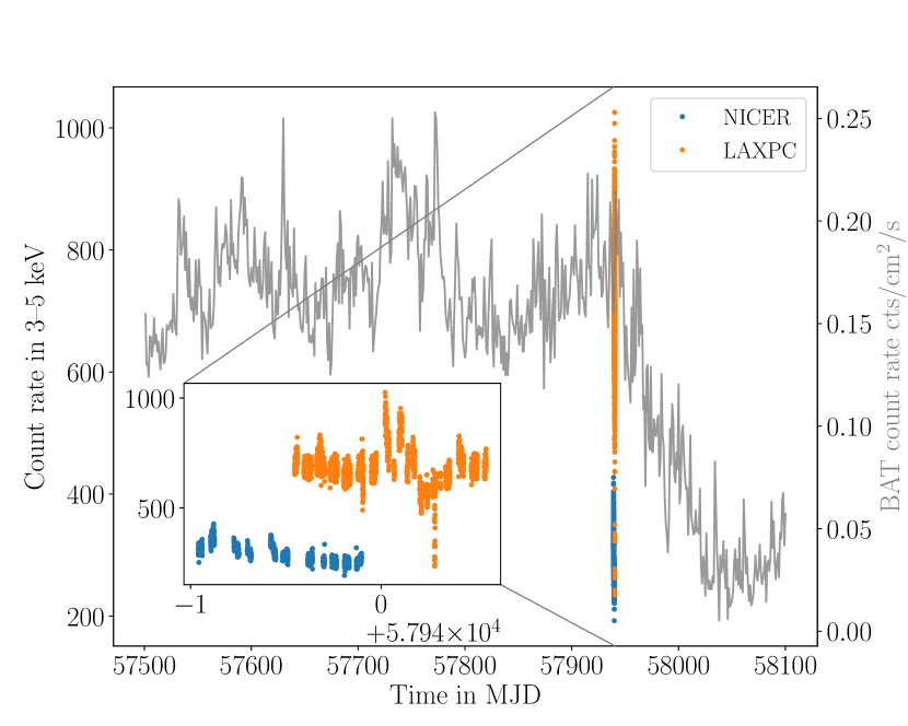
Figure 1: The NICER and LAXPC observation times are marked as blue and orange points in the Swift-BAT daily light curve of Cygnus X-1, highlighting that the simultaneous observations are made just before a state transition. The NICER and LAXPC count rates in 3–5 keV and binned at 16 s are shown in the inset (blue and orange points respectively), indicating a significant overlap in the two observations.

2.1 Data reduction

2.1.1 AstroSat-LAXPC

The data from LAXPC observations were reduced using the software LAXPCsoftware_May21 provided by the LAXPC Payload Operation Centre (POC). We used the tool laxpc_make_event to reduce the level 1 data to level 2 data, apply the calibration, and merge different orbits and observations into a single event file. We combined the two LAXPC observations into a single event file as NICER has simultaneous exposure with both of these and the observations themselves have a slight overlap which is taken into account by the laxpc_make_event tool during data reduction. The barycentric correction tool as1bary was utilised to convert the reference time frame from UTC to Solar system barycenter (TDB). The good time intervals (GTIs), light curves, spectra and background spectra were extracted by utilising the routines included in the software. The software also determines the appropriate response matrices for spectral fitting.The source had enough counts in each bin to use $\chi^{2}$ statistics but to account for the detector energy resolution ($\sim$10-15 %), we rebin the spectrum logarithmically with dE/E at 5% level.

2.1.2 NICER

The NICER data were downloaded from the HEASARC archive and were reduced using nicerl2 pipeline (distributed with HEASOFT version 6.29c) utilising the CALDB version xti20210707. The events from the detectors 14 and 34 were removed from the analysis as recommended by the instrument team. The barycentric correction was applied using the tool barycorr. The HEASOFT tool xselect was used to extract the light curves and spectra. The response and ancillary response files were extracted using the nicerrmf and nicerarf respectively. The background spectrum was computed using the tool nicer_bkg_estimator (v0p6) for the common interval, and the same background spectrum was used for each of the shot phases. We compared the background spectrum from an alternative tool nibackgen3C50 and found that the choice of the background model did not affect the results of the spectral fitting due to high count rate of the source. Hence we opted for the former tool. We rebinned the spectrum logarithmically and kept the number of bins similar to that for LAXPC so that the fitting is not dominated by the high number of degrees of freedom from the soft X-ray spectrum and is instead more sensitive to the changes in the high energy tail of the spectrum. This binning method is more conservative than the optimal binning routine suggested by the instrument team.

2.2 Shot selection

We verified that the time series have been correctly aligned after the barycentric correction so that we can detect and compare identical shots across the two instruments. Details of the verification are outlined in Appendix A.

For our study, we redefined the detection procedure of Yamada et al. (2013b). The brightness of the source and consequent high count rates in both LAXPC and NICER allowed us to use a finer temporal resolution of 0.05 s (compared to 0.1 s in Yamada et al. (2013b)) to detect the shots. Although the temporal resolution of both NICER and LAXPC is finer than 0.05 s, we prefer a minimum bin size of 0.05 s as the typical time lag at the Fourier frequencies >1 Hz is less than 0.05 s (Nowak et al., 1999; Uttley et al., 2011; De Marco et al., 2015) across different energy ranges. For a simultaneous detection of shots in LAXPC and NICER, we only considered the common interval across the light curves after barycentric correction. We utilised the light curves covering the complete operational energy range of each instrument for shot detection. We detected all the peaks in consecutive intervals of $t_{int}$ and determined the highest one. We selected a peak only if the peak count rate was at least $N$ times the local standard deviation above the local mean count rate (both determined from the segment of $t_{int}$) and separated from the previous selected peak by $M\times t_{int}$ ($M\geq$ 1). We verified our choice of the detection thresholds ($t_{int}$=10 s, $N$=3 and $M$=1) by varying them until the number of peak detections converged. For each peak, we extracted a segment of -10 to 10 s around the peak position and fit the segment with an exponential rise and decay function after subtracting the average of the count rate in the interval -10 to -4 and 4 to 10 s around the peak. The rise and decay timescales were allowed to vary independently, and the amplitude of both the exponential functions was tied together. To avoid spurious detections, we compared the parameters of each peak as seen by the independent detectors. We used light curves from LXP10 and 20 for parameter comparison. In the case of NICER, we divided the event file into two parts based on the detector ID and compared the light curves from each part. If the parameters of a peak in the two lightcurves were similar within 20% of the each other, then we classified the peak as a shot. As an additional test of our detection algorithm, we detected shots in LAXPC and NICER in 3–5 keV independently and tried various combinations of threshold parameters (viz. $t_{int}$, $N$ and $M$) to determine optimal detection of the shots. We find that similar peaks were being classified as shots but were detected at different significance as the mean count rate was dissimilar owing to different detector sensitivities. For the analysis, however, the full energy range in each instrument was chosen to detect and fit the shots.

In a common exposure of 6.39 ks, we detect 141 shots in LAXPC and 292 shots in NICER out of which 49 shots are exactly simultaneous (i.e. the peak time of shot lies within 0.05 s or the bin width of the lightcurve used). The differences in the number of shots detected in the two instruments is due to different operational energy ranges and the effects of Poisson variation.

To demonstrate the spectral dependence of the shots, we extracted the light curves in -4 to 4 s around each shot peak in various energy bands (3–5, 5–10, 10–20, 20–40 and 40–80 keV for LAXPC; 0.1–0.5, 0.5–1, 1–1.5, 1.5–3, 3–5 and 5–10 keV for NICER). We co-added the shot light curve by aligning the peaks and normalised the co-added peak with the average count rate from -4 to -2 and 2 to 4 s around the peak. The energy bands were picked in order to keep a similar mean count rate across different bands. We plot the shot profiles in figure 2. Noting that the most prominent variation is confined to -2–2 s around the peak, we split the profile in that interval into 9 equal width phase bins and extracted the corresponding GTI. The spectra were extracted for each GTI and fitted as described in section 2.4.

Figure 2: Co-added shot profiles for LAXPC (top panel) and NICER (bottom panel) in different energy bands are shown here. The energy ranges for each instrument are shown in different colours and markers and are indicated in the legend. The shots have been co-added by aligning the peaks and the profile has been normalised by the mean count rate in -4 to -2 and 2 to 4 s interval of the corresponding energy band. The co-adding was done for light curve binned at 0.05 s and was rebinned here (by a factor of 3 in both cases) for clarity. The dashed lines demarcate the interval probed using shot-phase resolved spectroscopy.

2.3 Time-averaged spectroscopy

To characterise the average behaviour of the source, we modelled the spectrum from 0.7–10 keV for NICER and 3.0–50.0 keV for LAXPC, beyond which the background counts were dominating the spectrum. We used a lower limit of 0.7 keV for the NICER spectrum as it is dominated by noise and forced trigger peaks in 0.1–0.7 keV band. We fit the spectra in xspec (version 12.12.0) using $\chi^{2}$ statistics. We tied the parameters across NICER and LAXPC spectra allowing for a cross normalisation constant. We used an extended energy range of 0.01–1000 keV with 10000 logarithmic bins for accurate computation of the convolution models.

Due to uncertainties in the calibration, we applied additional systematic errors to each spectrum (3% in LAXPC spectra and 1% in NICER spectra). The error bars reported throughout this work correspond to 1$\sigma$ confidence interval unless stated otherwise. We assumed that the system has a truncated thermalised disk and a comptonising cloud which intercepts a fraction of the disk photons and up-scatters them to produce the prominent powerlaw tail seen in the spectrum. We also included the interstellar absorption using the model tbabs using the abundances from Wilms et al. (2000) and cross section from Verner et al. (1996). The thermalised disk is modelled using kerrd while the thermal comptonisation was modelled using a convolution model thcomp (Zdziarski et al., 2020) using kerrd as an input. As an additional test, we used diskbb instead of kerrd and found that the fit was identical. However, for interpretation, we used kerrd as it incorporates the spectral hardening factor and gives a more accurate measurement of the inner disk radius. The model thcomp assumes a spherical geometry for the corona. We found that the assumed model is insufficient to explain the spectrum ($\chi^{2}$ of 561.3 for 123 degrees of freedom, dof) and the residuals indicated the presence of a reflection component. We modelled the reflection using the convolution model ireflect. The reflection is assumed to act only on the upscattered photons, while the combination of thcomp$\otimes$kerrd gives both the upscattered photons and the unscattered disk photons. Therefore we include the reflection component by removing the contribution of the unscattered photons from the thcomp$\otimes$kerrd and applying the convolution to the net model. On inclusion of the reflection component, the $\chi^{2}$ reduced to 160.7 for 119 dof. The residuals also indicated a presence of a iron emission line which was modelled phenomenologically with a gaussian line with a fixed width of 0.1 keV. After the inclusion of iron line, the $\chi^{2}$ reduced to an acceptable value of 132.2 for 117 dof. The best fit model can be written as tbabs$\times$(thcomp$\otimes$kerrd + gaussian + ireflect$\otimes($thcomp$\otimes$kerrd-constant$\times$kerrd)) where the constant is tied to 1-f; f being the fraction of photons up-scattered by thcomp. The parameters of all the instances of kerrd and thcomp were tied. The parameters for the fit of the time-averaged spectra are tabulated in Table 2, while the time-averaged spectrum and the residuals to the best fit model are shown in Figure 3.

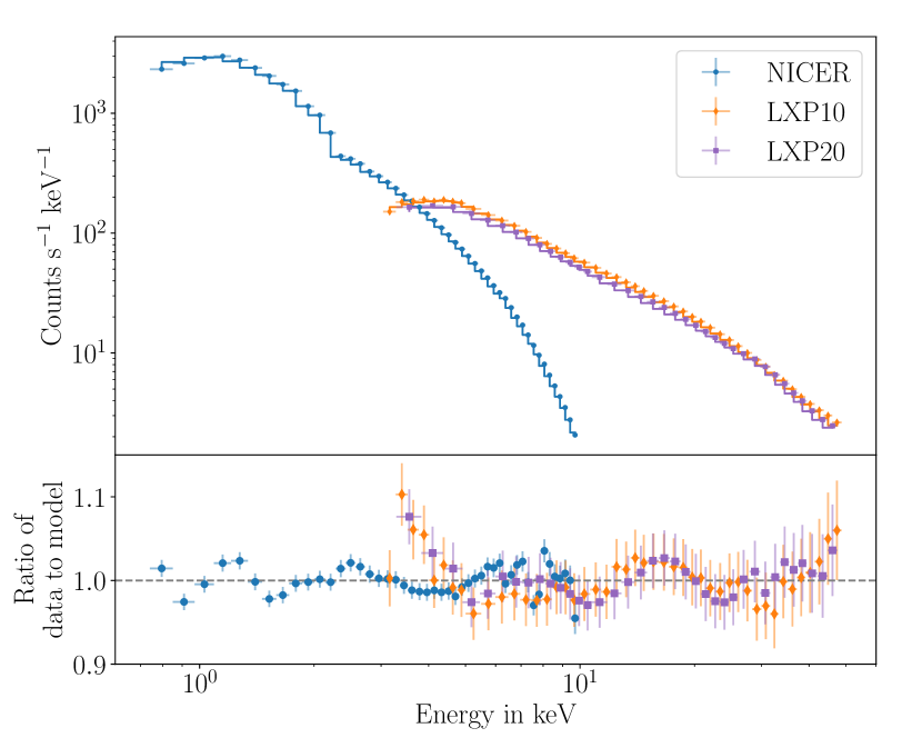
Figure 3: Time averaged spectrum, as observed by NICER and AstroSat-LAXPC, is shown here. The spectra have been logarithmically rebinned and fitted with tbabs$\times$(thcomp$\otimes$kerrd + gaussian + ireflect$\otimes($thcomp$\otimes$kerrd-constant$\times$kerrd)). The fitted parameters are tabulated in Table 2. Bottom panel shows the residuals in the form of ratio between the data to best fit model.

We fixed the source parameters to the values reported in the literature, i.e. the mass of the BH: 21.2 M_⊙, distance to the source: 2.2 kpc (Miller-Jones et al., 2021), the inclination of the disk: 40^∘ (Tomsick et al., 2014). We prefer the inclination value from the reflection measurement as compared to the orbital inclination, as it better represents the inner disk inclination. We fixed the spectral hardening factor of the disk to 1.7 (Shimura & Takahara, 1995). We applied a strict lower limit on R_in at 1.737 R_g as it corresponds to ISCO for a 21.2 M_⊙ BH with a spin of 0.97 (Miller-Jones et al., 2021). We found that the spectrum prefers an electron temperature (kT_e) beyond the operational range of LAXPC and since LAXPC has higher systematic uncertainties at higher energies, it cannot constrain the rollover in the spectrum. We thus froze the kT_e to 90 keV. For this kT_e, a corresponding optical depth ($\tau$) can be determined using equation 14 of Zdziarski et al. (2020) by switching the sign of the power law index ($\Gamma$) to a negative value in the model thcomp. The measurement of $\Gamma$ is robust, but the $\tau$ is dependent on the kT_e, and thus $\tau$ not be constrained with the current measurement.

Table 2: The best-fit parameter values for fitting of the time-averaged NICER and LAXPC spectra to the model tbabs$\times$(thcomp$\otimes$kerrd + gaussian + ireflect$\otimes($thcomp$\otimes$kerrd-constant$\times$kerrd)). The parameters of all instances of thcomp and kerrd are tied. We use the same model for shot resolved spectra. We find that, across the shot-resolved spectra, certain parameters (indicated below) are consistent with their time-averaged value within 1-2$\sigma$ confidence interval. We freeze kT_e at 90 keV as the spectra do not cover the requisite energy range to constrain the parameter.

Model	Parameter (Unit)	Value
tbabs	NH (1022 cm-2)	$0.576^{+0.006}_{-0.005}$*
kerrd	$\dot{\rm{M}}$ (1016 g/s): Accretion rate	$5.2^{+0.2}_{-0.1}$*
	Rin  (Rg): Inner radius	$6.7\pm 0.2$
gaussian	Line Energy	$6.41\pm 0.03$*
	Line width	$0.1^{\dagger}$
	Normalisation	$(1.9\pm 0.3)\times 10^{-3}$*
thcomp	$\Gamma$: Power law index	$1.918\pm 0.007$
	f: Scattering fraction	$0.432^{+0.005}_{-0.006}$
	kTe: Electron temperature (keV)	$90^{\dagger}$
ireflect	$\mathcal{R}$: Reflection fraction	$0.72\pm 0.04$*
	$\xi$: Ionisation parameter (erg cm/s)	$167^{+85}_{-55}$*
	Iron Abundance (solar units)	$5.5^{+0.8}_{-1.0}$*
	Abundance (solar units)	$8\pm 2$*
Flux	Disk Flux (ergs cm-2 s-1)	(1.259$\pm$0.001)$\times$10-8
	Heated Flux (ergs cm-2 s-1)	(2.191$\pm$0.002)$\times$10-8
	Reflected Flux (ergs cm-2 s-1)	(6.8$\pm$0.1)$\times$10-9
	CNICER	1.21$\pm 0.008$
	CLXP10	1.02$\pm 0.007$
	$\chi^{2}/dof$	132.2/117

Note: * The parameter was found consistent with time-averaged value across the shot profile

^† The parameter was kept frozen

2.4 Shot spectroscopy

The variation in the profile is well contained in the interval -2 to 2 s around the peak of the shot. To study the variation of the spectrum across the shot profile, we divided this interval into 9 uniform phase bins (labelled shot phase 0–8) and extracted the spectrum for each of the phase bins. We used an odd number of phase bins to contain the shot peak in the middle bin and ensure that a slight uncertainty in the determination of the peak does not affect the results. The phase-resolved spectra for the individual shot phases are shown in the top panel of figure 4. To highlight the spectral differences in a model independent way, the ratio of the spectra to phase 0 spectra are depicted in the bottom panel of figure 4. This also removes the instrumental effects and shows the changes in spectrum across the shot peak.

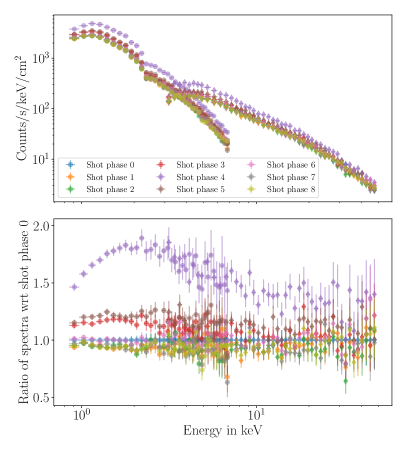
Figure 4: Spectrum for different shot phases as observed by LXP10 and NICER are shown in the top panel. To compare the spectra in a model independent way, we also include the ratio of the spectra to the phase-0 spectra in the bottom panel. The spectra for phase 3-5 show clear deviation from 1.0 and spectra for phase 4 show a spectral peak close to 2 keV indicating definite spectral evolution across the shot peak.

The spectrum from each phase bin was fitted with the same model as the time-averaged spectrum to study the evolution of the spectral parameters. We froze the iron line parameters for each shot phase to the values suggested by the time-averaged spectrum as the iron line is weakly detected in each shot phase. Leaving all the parameters mentioned in table 2 (except kT_e) free, we found that many of the parameters are consistent with the time averaged results within 1-2$\sigma$ confidence level. These parameters include reflection fraction ($\mathcal{R}$), Hydrogen column density (N_H), iron abundance, metal abundance and disk ionisation ($\xi$). On freezing these parameters, the $\chi^{2}$ increases by $\sim$15 for additional 5 degrees of freedom per shot phase spectrum, favouring a simpler model (i.e. the one with fewer parameters free). After fixing these parameters, we determined the minimum parameters required to explain the spectral changes across the shot by following the methodology outlined in the appendix C. We find that only $\Gamma$, f and inner disk radius (R_in) are changing significantly across the shot profile with mass accretion rate ($\dot{\rm{M}}$) being consistent with the time averaged value. The variation of $\Gamma$, f and R_in after freezing the rest of the parameters to their time-averaged values is shown in figure 5. The parameter value corresponding to the time-averaged spectrum is indicated as a dashed black line with the shaded region marking the 1$\sigma$ confidence interval reported in Table 2. Appendix D discusses the degeneracy in determining the value of the key parameters (viz. $\Gamma$, f and R_in) for individual shot phases.

Figure 5: The variation of parameters ($\Gamma$, f, and R_in in top, middle and bottom panels respectively) is shown here. The shot profile corresponds to the interval from -2 to 2 s in figure 2 and is divided into 9 equal phase bins labelled 0–8. The rest of the parameters are found to be consistent with the time-averaged value (within 1$\sigma$) are frozen to that value (see Table 2 for the values of the parameters) and see figure 10 for the variation in the $\chi^{2}$ as a function of shot phase. The dashed line is the value of the parameter as observed in the time-averaged spectrum, with the shaded region indicating the 1$\sigma$ confidence interval.

For the observations analysed, we find that the degeneracy between the variation in kT_e and $\tau$ cannot be broken. To probe the degeneracy, we determined the variation in $\tau$ and kT_e independently keeping the other parameter fixed. The variation in $\tau$ was tested by keeping kT_e fixed at 90 keV (as done in time-averaged analysis). On the other hand, the variation in kT_e was tested by fixing $\tau$ for all the phases at the value observed in shot phase 4 (i.e. the peak of the shot) for kT_e= 90 keV. In both cases the parameter was observed to reach a minimum at the shot peak and the value of the parameter dropped by $\sim$15% at the shot peak. We also computed the $\chi^{2}$ by varying $\tau$ and kT_e in a grid slightly larger than the variation observed in the top panel of figure 6. The contours of the $\chi^{2}$ variation for two shot phases (0 and 4) are shown in bottom panel of the figure 6.

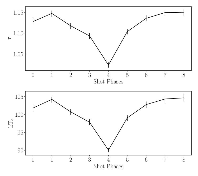
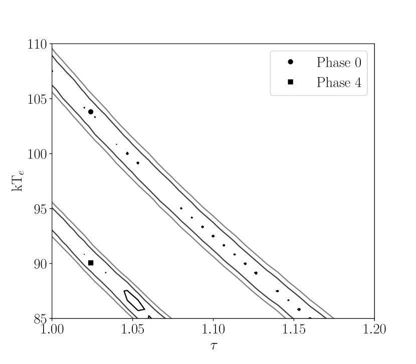
Figure 6: Testing the degeneracy between the $\tau$ and kT_e. In the top panel, the variation of the $\tau$ is allowed to vary across the shot phases while the electron temperature is kept fixed at 90 keV. In the middle panel, the $\tau$ is kept fixed at the value obtained for the peak of the shot (i.e. phase 4) and the electron temperature is allowed to vary. In the bottom panel, the contour plots are shown for simultaneous variation of the $\chi^{2}$ probing different $\tau$ and kT_e. For clarity, the contour plots are shown only for two shot phases 0 and 4. The filled circle and square in the bottom panel indicate the $\chi^{2}$ contour corresponding to phase 0 and 4 respectively. The degeneracy between the parameters is clearly visible which cannot be mitigated without a high energy spectrum to constrain the rollover.

We computed the fluxes from the disk and the comptonised region using cflux model in xspec. The fluxes were determined in 0.1–500 keV band by applying cflux on kerrd and thcomp$\otimes$(kerrd). The difference in the two fluxes corresponds to the amount of heat supplied by the comptonising medium. We also computed the flux from the reflection component by applying cflux on the ireflect$\otimes($thcomp$\otimes$kerrd-constant*kerrd). The variation of the fluxes as a function of the shot phases is shown in figure 7. The fluxes are normalised to the corresponding value obtained from the time-averaged spectrum to highlight the variation better.

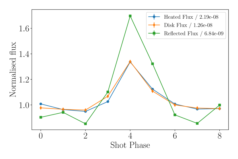
Figure 7: The variation of the flux of different spectral components across the shot profile is shown here. To highlight the relative variation, the fluxes have been normalised by the value mentioned in the legend. The heated flux is obtained from difference of cflux on thcomp$\otimes$(gaussian+kerrd) and cflux on kerrd. The disk flux is obtained from cflux on kerrd. The iron line component is constant across the shot profile and the flux contribution from is about 2 orders lower than the measured disk flux. The heated flux is heating provided by the comptonising medium and is computed by subtracting the previous fluxes. The fluxes also follow the show profile indicating that during the shot, both fluxes from the disk and the heating provided by the comptonising cloud rises.

3 Results and Discussion

Using simultaneous observation of AstroSat and NICER, we study the spectral properties of Cyg X-1. The variability in Cyg X-1 is known to span decades in frequency (see Maqbool et al., 2019, for example) and is coupled across different frequency regimes (Uttley et al., 2005). In this work, we devise a peak isolation technique based on the procedure outlined in Yamada et al. (2013b) to identify and characterise some of the variability in Cyg X-1. In a common exposure of 6.39 ks, we detect 49 simultaneous peaks in LAXPC and NICER which we characterise as shots by comparing the properties of the peak across independent lightcurves and across different instruments. Compared to Yamada et al. (2013b), we detect far fewer shots. We attribute this to our strict constraint of simultaneous detection of peaks in LXP10, LXP20 and NICER with near-identical shape (quantified by the fitting of each peak and comparing the parameters across the independent detectors). These shots represent the brightest and most prominent peaks in the lightcurve detected in a wide energy range (see Appendix B for a comparison between cross-correlation functions from shot intervals and complete lightcurve). The variation of the shot profile across different energies as seen by LAXPC is quite similar to that observed by Yamada et al. (2013b) and Liu & Li (2004). These authors have also observed a decrease in the relative shot peak amplitude with energy and thus a sharper dip in the ratio profile. The profile of the shots in soft X-rays, observed for the first time with NICER, paints a slightly different picture. The relative peak height is the smallest at the lowest energy bin 0.1–1 keV, rises till 2 keV and then drops again (see the ratio plot in figure 4). This is similar to the peaking of the relative shot profile (at $\sim$10 keV) as observed by Liu & Li (2004) for the HSS shot analysis. The timescales seen in the NICER profile follow similar trends as seen in the LAXPC data. The differences in the relative amplitude and in the ratio of the shot resolved spectra point to spectral changes in the source in the timescale of the shot. Due to a fewer number of shots detected, we are unable to reproduce the asymmetric shot ratio profile observed in Yamada et al. (2013b).

3.1 Time averaged results

We model the time-averaged spectra using a thermalised accretion disk with a comptonising cloud of hot electrons up-scattering a fraction of the disk photons and the emission from the comptonising cloud then reflected from the cool disk. Additionally, we find evidence of a broad iron line, which has been reported previously (Makishima et al., 2008; Duro et al., 2016; Walton et al., 2016). We find that the absorption column density of neutral hydrogen is $\sim$5.7$\times 10^{21}$ cm^-2. Parker et al. (2015), Walton et al. (2016) and Basak et al. (2017) have observed an N_H of 4–7$\times 10^{21}$ cm^-2 for different epochs of the source indicating a variable nature of the absorption column due to the stellar winds in the source. We observe a truncated disk ($\sim$6.7 R_g) with a $\dot{\rm{M}}$ of 5.2$\times 10^{16}$ g/s. The R_in measurement is larger than the one seen in Parker et al. (2015) but smaller than that of Basak et al. (2017). An important caveat regarding the measurement of the inner disk radius is that it depends significantly on the assumed mass of the BH. The measurements by Parker et al. (2015), Duro et al. (2016), Basak et al. (2017) and Axelsson & Done (2018) have assumed 14.8 M_⊙ BH (Orosz et al., 2011) which would lead to a higher estimate of inner truncation radius. For example, the inner radius computed from the diskbb normalisation from Duro et al. (2016) is $\sim$99 km (or $\sim$3.17 R_g; after incorporating the spectral hardening factor of 1.7). For a BH of 21.2 M_⊙ at a distance of 2.2 kpc (Miller-Jones et al., 2021) the same measurement becomes consistent with our result. Furthermore, Basak et al. (2017) emphasise that the measurement of the inner disk radius depends strongly on the continuum assumed.

The powerlaw tail is modelled with thermal comptonisation by a spherical corona with a high electron temperature. We find that typically 40% of the photons from the disk are intercepted by the comptonising medium. Parker et al. (2015) find that the spectral cutoff in the Suzaku spectrum is observed at about 100 keV. This is beyond the energy range of LAXPC, and due to reduced sensitivity at higher energies, we are unable to constrain the electron temperature. We find that for a fiducial value of 90 keV, we get an acceptable fit to the spectrum. We obtain a significant reflection fraction ($0.43^{+0.005}_{-0.006}$), which is consistent with Makishima et al. (2008). Different studies have shown different measurements of the reflection fraction (Tomsick et al., 2014; Parker et al., 2015; Duro et al., 2016; Basak et al., 2017), which could be attributed to a source evolution or differences in the assumptions of the models or differences in the interpretation of the reflection fraction (e.g. Dauser et al., 2016). Additionally, Parker et al. (2015) note a degeneracy between the reflection fraction and the iron abundance. We observe that the disk is weakly ionised similar to Makishima et al. (2008) but in contrast to the high ionisation observed in Tomsick et al. (2014), Parker et al. (2015), Duro et al. (2016), Walton et al. (2016) and Basak et al. (2017). We observe supersolar iron abundance in the source, which has also been previously reported (Parker et al., 2015; Duro et al., 2016; Basak et al., 2017). While Makishima et al. (2008) and Basak et al. (2017) both require two-component comptonisation models to fit the high-resolution spectrum from Suzaku and Suzaku-NuSTAR observations, we find that an adequate fit can be obtained with a single comptonising zone.

3.2 Variation of parameters across the shot

Across the shot, we observe that N_H, $\dot{M}$, abundances, $\xi$, and $\mathcal{R}$ are consistent with the values observed in the time-averaged spectra. The spectral parameters $\Gamma$, f and R_in of the phase bins 0–2 and 6–8 are close to the time-averaged parameters indicating that the processes corresponding to the shot are limited to phase bins 3–5 (i.e. -0.833–0.833 s around the shot peak). Within the reduced interval, $\Gamma$ and f rise as the shot peak approaches and decay after the peak. The inner disk radius, however, reduces as the shot peak approaches and then rises back to the time-averaged value as the shot decays. Across the shot, the accretion rate of the system is consistent within 4% of the measured value. Yamada et al. (2013b) have described the shot phenomenon in 10–200 keV energy range, which is primarily dominated by the emission from the comptonising region and the reflection. Thus assuming a near symmetric inflow of soft photons, the authors have described that due to the asymmetric response of the comptonising region (i.e. electron temperature and optical depth), the hardness ratio of the shot is asymmetric. In our work, we have compared the shots in the complementary energy range of 0.1–80 keV and observed that the shot profiles are indeed symmetric. Due to a lack of sensitivity and energy coverage at hard X-rays, we are unable to observe the asymmetric ratio profiles and the observed variation in both electron temperature and optical depth. Combining the results of Yamada et al. (2013b) and present work, we describe the shot phenomenon as follows. At a constant accretion rate, the disk moves suddenly inwards, heating up in the process. As the temperature rises, the emission from the disk increases (as evident from the variation of the flux, Figure 7). The surge of photons then interacts with the comptonising medium causing a change in the powerlaw index, which is a manifestation of a simultaneous change in optical depth and electron temperature as shown by Yamada et al. (2013b). We also note that during the shot, the fraction of photons intercepted by the comptonising medium also increases and then decreases, possibly related to the change in the inner radius of the disk. The flux contributions of the disk and the comptonising medium are observed to mimic the shot profile.

For an accretion disk, the thermal timescale at a particular radius can be estimated by calculating the disk parameters from the observed physical parameters. A rough estimate indicates that the thermal timescale at 6.7 R_g is about 0.14 s, which is faster than the timescales in which shot occurs. This indicates that our assumption of the thermalised disk is valid even for each shot phase.

The inward and outward motion of the disk is observed to happen within a few seconds, with the accretion rate remaining constant within 4%. The inward/outward motion of the disk is often assumed to be the difference between different states of Cyg X-1 (Done et al., 2007) and is usually linked with the changes in the accretion rate. Meyer et al. (2007) and Taam et al. (2018) have described the phenomenon with condensation/evaporation of the matter in the comptonising medium onto the accretion disk. Although the processes described in these works are used to model the transition between different spectral states of the source, a temporary condensation/evaporation could also explain the motion of the inner disk without a change in the accretion rate. Detailed calculations regarding this mechanism is beyond the scope of this work.

4 Conclusions

We probe the peaking features observed in Cyg X-1 in 0.1–80 keV energy range using high time resolution instruments LAXPC and NICER. Our results can be summarised as follows:

1. Observation of the shot profile in soft energy bands for the first time: The shot profile in different energy bands in soft X-rays was observed for the first time using the NICER observation. The shot profile indicates that the variation of the relative amplitude of the shot peak is not monotonic, and the amplitude is maximum at $\sim$2 keV energy bands.

2. Measurement of inner radius: Assuming a thermalised disk with a spherical corona up-scattering a fraction of photons and reflection of the comptonised photons from the disk, we measure the inner truncation radius at 6.7$\pm 0.2$ R_g.

3. Origin of the photon surge: Using the wideband simultaneous coverage, we fit the shot-phase resolved spectra and determine that the sudden spike in the count rate is related to the inward motion of the inner edge of the disk, which leads to a larger fraction of photons being scattered and a subsequent cooling of the electron cloud.

Data availability

The NICER data is available at https://heasarc.gsfc.nasa.gov/docs/archive.html. The AstroSat data is available at https://astrobrowse.issdc.gov.in/astro_archive/archive/Home.jsp. In both cases, the datasets can be searched in the respective websites using the observation IDs listed in Table 1.

Appendix A Matching LAXPC and NICER times

To have identical detection of shots across two different instruments it is paramount to verify if the variability across the detectors is identical. To verify if we have successfully aligned the time series, we computed the cross-correlation between the light curves of the same binning from LAXPC and NICER in the same energy range (4–8 keV). We ensured that only the exact simultaneous light curves are being cross-correlated by creating standard Good Time Intervals (GTIs) using the tools provided by the instrument team (laxpc_make_stdgti for LAXPC and nimaketime for NICER). The standard GTI were then merged using the ftool ftmgtime with "AND" option. The cross correlation for light curves of different time resolutions is found to peak at zero lag. The peak of the correlation was fitted with two Gaussians. The peak of both Gaussians are consistent with zero within 2$\sigma$ ($(-3.2\pm 2.02)\times 10^{-3}$ s and $(-4.93\pm 4.93)\times 10^{-4}$ s for orange and green curves in figure 8 top panel respectively).

We also computed the coherence as a function of Fourier frequencies and computed the phase lags (Nowak et al., 1999). For a identical detection the phase lags should be consistent with zero. The time lag in the frequency range 0.1–20 Hz is consistent with zero within 2$\sigma$ ((-7.2$\pm 4.6$)$\times 10^{-4}$ s, see figure 8 bottom panel). The value of the lag is much smaller than minimum time bin used in the analysis and thus we assume that the observations have been successfully aligned.

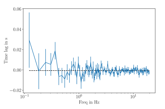
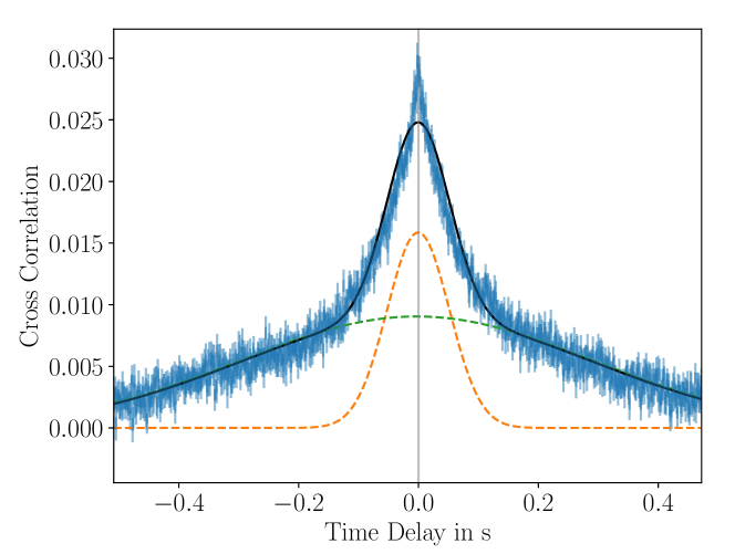
Figure 8: Cross correlation (top panel) and Frequency dependent time lag (bottom panel) between NICER and LAXPC 4–8 keV. The cross correlation function has been fitted with two Gaussian functions of different width (shown as orange and green dashed lines). The combined model is shown as black curve. The peaks of both functions are consistent with 0.0 within 2$\sigma$. The frequency dependent time lags were fitted with a constant which is also consistent with 0.0 within 2$\sigma$.

Appendix B Variability of the shot intervals vs variability in the full lightcurve

To determine if the intrinsic variability during the shot interval is significantly different from the general aperiodic variability, we computed cross-correlation functions during shot intervals and the full lightcurve between extreme energy bands (0.5–1.5 keV for NICER and 15–60 keV for LAXPC, see figure 9). We find that the CCFs are significantly different indicating that the variability probed by the brightest and most significant shots represents a part of the general aperiodic variability.

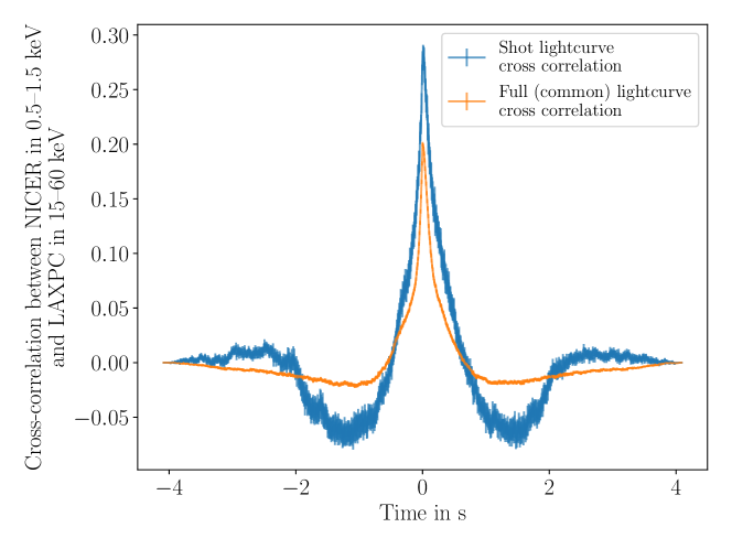
Figure 9: Cross-correlation function (CCF) between NICER lightcurve in 0.5–1.5 keV and LAXPC lightcurve in 15–60 keV. The CCF for the shot lightcurves is shown in blue while the CCF for the common lightcurve is shown in orange. The CCFs differ significantly for different time delays but peak at 0.0 s.

Appendix C Determining minimum number of parameters for shot spectroscopy

To determine the minimum number of parameters which could explain the spectral changes during the shot we observed the variation in the $\chi^{2}$ by varying different combinations of the $\Gamma$, f, R_in and $\dot{\rm{M}}$ and keeping the rest fixed to the value suggested in the time averaged fits (table 2). The variations of the $\chi^{2}$ and the corresponding degrees of freedom are shown in figure 10. A high $\chi^{2}$ is indicative of a bad fit and therefore assumed model being insufficient to explain the variation. In all cases (except one) tested like this, we find that the $\chi^{2}$ is high at the shot peak and in single parameter cases, it is unacceptable for shot phases 3 and 5. The only case where the $\chi^{2}$ is acceptable for all cases, is when $\Gamma$, scattering fraction (f) and inner disk radius (R_in) are left free and ($\dot{\rm{M}}$) is kept fixed at time-averaged value.

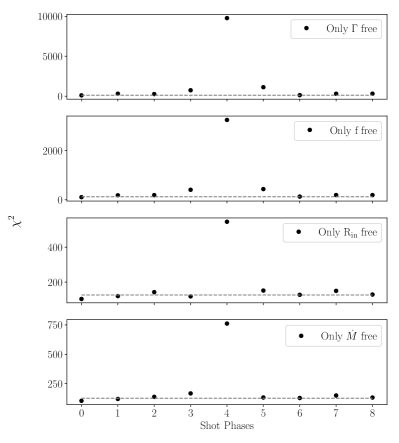
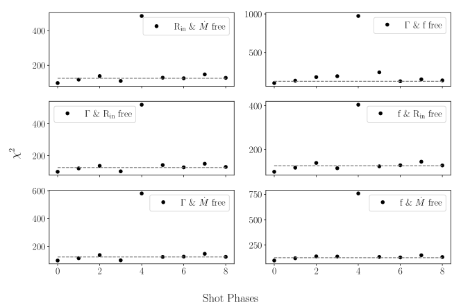
Figure 10: Variation of Best-fit $\chi^{2}$ as a function of shot phase while keeping various combinations of parameters free. The $\chi^{2}$ values are shown as black dots while the degrees of freedom are shown as a grey dashed line. The parameter(s) kept free are indicated in the legend of respective panels.

Appendix D Probing degeneracy between $\Gamma$, f and R_in

For each shot-phase spectrum, we sampled the $\chi^{2}$ function by allowing $\Gamma$, f and R_in to vary. The parameter space was sampled using a Markov Chain Monte Carlo sampler with Goodman-Weare algorithm. We initialised 50 walkers for 1000 steps each (after removing 100 steps corresponding to the burn-in period). The walkers were initialised using the parameter values and the covariance matrix obtained after fitting the spectra in xspec. The 2D and 1D distribution of the parameters are shown as a corner plot (Foreman-Mackey, 2016) for some of the shot phases in figure 11.

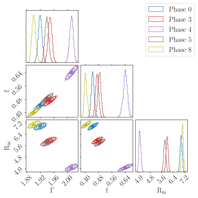
Figure 11: 1D and 2D distribution of the parameters for different shot phases. The distribution is shown only for five shot phases for clarity. The colour scheme is kept consistent with figure 4.

References

- Antia et al. (2017) Antia H. M., et al., 2017, ApJS, 231, 10
- Axelsson & Done (2018) Axelsson M., Done C., 2018, MNRAS, 480, 751
- Basak et al. (2017) Basak R., Zdziarski A. A., Parker M., Islam N., 2017, MNRAS, 472, 4220
- Dauser et al. (2016) Dauser T., García J., Walton D. J., Eikmann W., Kallman T., McClintock J., Wilms J., 2016, A&A, 590, A76
- De Marco et al. (2015) De Marco B., Ponti G., Muñoz-Darias T., Nandra K., 2015, ApJ, 814, 50
- Done et al. (2007) Done C., Gierliński M., Kubota A., 2007, A&ARv, 15, 1
- Duro et al. (2016) Duro R., et al., 2016, A&A, 589, A14
- Fabian et al. (2012) Fabian A. C., et al., 2012, MNRAS, 424, 217
- Feng et al. (1999) Feng Y. X., Li T. P., Chen L., 1999, ApJ, 514, 373
- Foreman-Mackey (2016) Foreman-Mackey D., 2016, The Journal of Open Source Software, 1, 24
- Gendreau et al. (2016) Gendreau K. C., et al., 2016, in Space Telescopes and Instrumentation 2016: Ultraviolet to Gamma Ray. p. 99051H, doi:10.1117/12.2231304
- Li & Fenimore (1996) Li H., Fenimore E. E., 1996, ApJ, 469, L115
- Lightman & White (1988) Lightman A. P., White T. R., 1988, ApJ, 335, 57
- Liu & Li (2004) Liu C. Z., Li T. P., 2004, ApJ, 611, 1084
- Makishima et al. (2008) Makishima K., et al., 2008, PASJ, 60, 585
- Maqbool et al. (2019) Maqbool B., et al., 2019, MNRAS, 486, 2964
- Meyer et al. (2007) Meyer F., Liu B. F., Meyer-Hofmeister E., 2007, A&A, 463, 1
- Miller-Jones et al. (2021) Miller-Jones J. C. A., et al., 2021, Science, 371, 1046
- Negoro et al. (1994) Negoro H., Miyamoto S., Kitamoto S., 1994, ApJ, 423, L127
- Negoro et al. (2001) Negoro H., Kitamoto S., Mineshige S., 2001, ApJ, 554, 528
- Nowak et al. (1999) Nowak M. A., Vaughan B. A., Wilms J., Dove J. B., Begelman M. C., 1999, ApJ, 510, 874
- Orosz et al. (2011) Orosz J. A., McClintock J. E., Aufdenberg J. P., Remillard R. A., Reid M. J., Narayan R., Gou L., 2011, ApJ, 742, 84
- Parker et al. (2015) Parker M. L., et al., 2015, ApJ, 808, 9
- Poutanen & Svensson (1996) Poutanen J., Svensson R., 1996, ApJ, 470, 249
- Shakura & Sunyaev (1973) Shakura N. I., Sunyaev R. A., 1973, A&A, 500, 33
- Shimura & Takahara (1995) Shimura T., Takahara F., 1995, ApJ, 445, 780
- Singh et al. (2014) Singh K. P., et al., 2014, in Space Telescopes and Instrumentation 2014: Ultraviolet to Gamma Ray. p. 91441S, doi:10.1117/12.2062667
- Taam et al. (2018) Taam R. E., Qiao E., Liu B. F., Meyer-Hofmeister E., 2018, ApJ, 860, 166
- Tomsick et al. (2014) Tomsick J. A., et al., 2014, ApJ, 780, 78
- Tomsick et al. (2018) Tomsick J. A., et al., 2018, ApJ, 855, 3
- Uttley et al. (2005) Uttley P., McHardy I. M., Vaughan S., 2005, MNRAS, 359, 345
- Uttley et al. (2011) Uttley P., Wilkinson T., Cassatella P., Wilms J., Pottschmidt K., Hanke M., Böck M., 2011, MNRAS, 414, L60
- Verner et al. (1996) Verner D. A., Ferland G. J., Korista K. T., Yakovlev D. G., 1996, ApJ, 465, 487
- Walton et al. (2016) Walton D. J., et al., 2016, ApJ, 826, 87
- Wilms et al. (2000) Wilms J., Allen A., McCray R., 2000, ApJ, 542, 914
- Yadav et al. (2016) Yadav J. S., et al., 2016, in Space Telescopes and Instrumentation 2016: Ultraviolet to Gamma Ray. p. 99051D, doi:10.1117/12.2231857
- Yamada et al. (2013a) Yamada S., Makishima K., Done C., Torii S., Noda H., Sakurai S., 2013a, PASJ, 65, 80
- Yamada et al. (2013b) Yamada S., Negoro H., Torii S., Noda H., Mineshige S., Makishima K., 2013b, ApJ, 767, L34
- Zdziarski et al. (2020) Zdziarski A. A., Szanecki M., Poutanen J., Gierliński M., Biernacki P., 2020, MNRAS, 492, 5234
- Zhao et al. (2020) Zhao X.-S., et al., 2020, Journal of High Energy Astrophysics, 27, 53