∎

Condensed interior-point methods: porting reduced-space approaches on GPU hardware

Abstract

The interior-point method (IPM) has become the workhorse method for nonlinear programming. The performance of IPM is directly related to the linear solver employed to factorize the Karush–Kuhn–Tucker (KKT) system at each iteration of the algorithm. When solving large-scale nonlinear problems, state-of-the art IPM solvers rely on efficient sparse linear solvers to solve the KKT system. Instead, we propose a novel reduced-space IPM algorithm that condenses the KKT system into a dense matrix whose size is proportional to the number of degrees of freedom in the problem. Depending on where the reduction occurs we derive two variants of the reduced-space method: linearize-then-reduce and reduce-then-linearize. We adapt their workflow so that the vast majority of computations are accelerated on GPUs. We provide extensive numerical results on the optimal power flow problem, comparing our GPU-accelerated reduced space IPM with Knitro and a hybrid full space IPM algorithm. By evaluating the derivatives on the GPU and solving the KKT system on the CPU, the hybrid solution is already significantly faster than the CPU-only solutions. The two reduced-space algorithms go one step further by solving the KKT system entirely on the GPU. As expected, the performance of the two reduction algorithms depends intrinsically on the number of available degrees of freedom: their performance is poor when the problem has many degrees of freedom, but the two algorithms are up to 3 times faster than Knitro as soon as the relative number of degrees of freedom becomes smaller.

1 Introduction

Most optimization problems in engineering consist on minimizing a cost subject to a set of equality constraints that represent the physics of the problem. Often, only a subset of the problem variables are actionable. A particular instance of these types of problems is the Optimal Power Flow (OPF), which formulates as a large-scale nonlinear nonconvex optimization problem. It is one of the critical power system analysis carried out multiple times per day by any electrical power system market operator frank2012optimal . In brief, it selects the optimal real power of dispatchable resources (typically power plants) subject to physical constraints (the power flow constraints, or power balance), and operational constraints (e.g voltage or line flow limits) cain2012history . It is challenging to solve to optimality, particularly since its solution is needed within a prescribed and fairly tight time limit. Since the 1990s, the efficient solution of OPF has relied on the interior-point method (IPM). In particular, state-of-the-art numerical tools developed for sparse IPMs can efficiently handle the sparse structure of typical OPF problems. At each iteration of the IPM algorithm, the descent direction is computed by solving a Karush–Kuhn–Tucker (KKT) system, which requires the factorization of large-scale ill-conditioned unstructured symmetric indefinite matrices nocedal_numerical_2006 . For that reason, current state-of-the-art OPF solvers combine a mature IPM solver wachter2006implementation ; waltz2006interior together with a sparse Bunch–Kaufman factorization routine duff2004ma57 ; schenk2004solving . Along with an efficient evaluation of the derivatives, this method is able to solve efficiently OPF problems with up to 200,000 buses on modern CPU architectures kardos2018complete .

1.1 Interior-point method on GPU accelerators: state of the art

Most upcoming HPC architectures are GPU-centric, and we can leverage these new parallel architectures to solve very-large OPF instances. However, porting IPM to the GPU is nontrivial because GPUs are based on a different programming paradigm from that of CPUs: instead of computing a sequence of instructions on a single input (potentially dispatched on different threads or processes), GPUs run the same instruction simultaneously on hundreds of threads (SIMD paradigm: Single Instruction, Multiple Data). Hence, GPUs shine when the algorithm can be decomposed into simple instructions running entirely in parallel where the same instruction is executed on different data in lockstep (as is the case for most dense linear algebra). In general, not all algorithms are fully amenable to this paradigm. One notorious example is branching in the control flow: when the instructions have multiple conditions, dispatching the operations on multiple threads makes execution in lockstep impossible.

Unfortunately, factorization of unstructured sparse indefinite matrix is one of these edge cases: unlike dense matrices, sparse matrices have unstructured sparsity, rendering most sparse algorithms difficult to parallelize. Thus, implementing a sparse direct solver on the GPU is nontrivial, and the performance of current GPU-based sparse linear solvers lags far behind that of their CPU equivalents swirydowicz2021linear ; tasseff2019exploring . Previous attempts to solve nonlinear problems on the GPU have circumvented this problem by relying on iterative solvers cao2016augmented ; schubiger2020gpu or on decomposition methods kim2021leveraging . Here, we have chosen instead to revisit the original reduced-space algorithm proposed in dommel_optimal_1968 : this method condenses the KKT system into a dense matrix, whose size is small enough to be factorized efficiently on the GPU with dense direct linear algebra.

1.2 Reduced-space interior-point method

Reduced-space algorithms have been studied for a long time. In dommel_optimal_1968 the authors introduced a reduced-space algorithm, one of the first effective methods to solve the OPF problem. The method has several first-order variants, known as the generalized reduced-gradient algorithm abadie1969carpentier or the gradient projection method rosen1961gradient , whose theoretical implications are discussed in gabay1982minimizing . The extension of the reduced-space method to second-order comes later sargent1974reduced —as well as its application to OPF burchett1984quadratically —the method becoming during the 1980s a particular case of the sequential quadratic programming algorithm coleman1982nonlinear ; fletcher2013practical ; nocedal1985projected ; gurwitz1989sequential . However, the (dense) reduced Hessian has always been challenging to form explicitly, favoring the development of approximation algorithms for second-order derivatives, based on quasi-Newton biegler1995reduced or on Hessian-vector products biros_parallel_2005 . The reduced-space method was extended to IPM in the late 1990s cervantes2000reduced and was already adopted to solve OPF jiang2010reduced . We refer to kardos2020reduced for a recent report describing the application of reduced-space IPM to OPF.

1.3 Contributions

Our reduced-space algorithm is built on this extensive previous work. In Section 2 we propose a tractable reduced-space IPM algorithm, allowing the OPF problem to be solved entirely on the GPU. Instead of relying on a direct sparse solver, our reduced-space IPM condenses the KKT system into a dense linear system whose size depends only on the number of control variables in the reduced problem (here the number of generators). When the number of degrees of freedom is much smaller than the total number of variables, the KKT system size can be dramatically reduced. In addition, we establish a formal connection between the reduced IPM algorithm and the seminal reduced-gradient method of Dommel and Tinney dommel_optimal_1968 . Depending on whether the reduction occurs at the KKT system level or directly at the nonlinear level, we propose two different reduced-space algorithms: Linearize-then-reduce and Reduce-then-linearize. We describe a parallel implementation of the reduction algorithm in Section 3 and show how we can exploit efficient linear algebra kernels on the GPU to accelerate the algorithm. We discuss an application of the proposed method to the OPF problem in Section 4: our numerical results show that both the reduced IPM and its feasible variant are able to solve large-scale OPF instances—with up to 70,000 buses—entirely on the GPU. This result improves on the previous results reported in kardos2020reduced ; pacaud2021feasible . As expected, the reduced-space algorithm is competitive when the problem has fewer degrees of freedom, but it achieves respectable performance (within a factor of 3 compared with state-of-the-art methods) even on the less favorable instances. To the best of our knowledge, this is the first time a second-order GPU-based NLP solver matches the performance of state-of-the art CPU-based solvers on the resolution of OPF problems.

2 Reduced interior-point method

In §2.1 we introduce the problem formulation under consideration. In this problem the independent variables (the control, associated to the problem’s degrees of freedom) are split from the dependent variables (the state). The reduction is akin to a Schur complement reduction and can occur at the linear algebra or the nonlinear levels. In §2.2 we present our first method, linearize-then-reduce, performing the reduction directly on the KKT system. In §2.3 we show that we can reduce equivalently the nonlinear model using the implicit function theorem, giving our second method: reduce-then-linearize.

2.1 Formalism

The problem we study in this section has a particular structure: the optimization variables are divided into a control variables $\bm{u}\in\mathbb{R}^{n_{u}}$ and a state variables $\bm{x}\in\mathbb{R}^{n_{x}}$. The control and the state variables are coupled together via a set of equality constraints:

$$g(\bm{x},\bm{u})=0\,,$$ (1)

with $g:\mathbb{R}^{n_{x}}\times\mathbb{R}^{n_{u}}\to\mathbb{R}^{n_{x}}$ (note that we choose the dimension of the output space to be equal to $n_{x}$, the dimension of the state). The function $g$ is often related to the physical equations of the problem; and, depending on the applications, it can encode balance equations (optimal power flow, the primary object of study in this work), but also discretizations of dynamics (optimal control), or partial differential equations (PDE-constrained optimization).

We call Equation (1) the state equation of the problem. Further, an objective function $f:\mathbb{R}^{n_{x}}\times\mathbb{R}^{n_{u}}\to\mathbb{R}$ and a set of generic constraints $h:\mathbb{R}^{n_{x}}\times\mathbb{R}^{n_{u}}\to\mathbb{R}^{m}$ are given. The optimization problem in state-control form can be expressed as

$$\min_{\bm{x},\bm{u}}\;f(\bm{x},\bm{u})\quad\text{subject to}\quad\left\{\begin{aligned} &\bm{u}\geq 0\;,\quad\bm{x}\geq 0\;,\\ &g(\bm{x},\bm{u})=0\;,\quad h(\bm{x},\bm{u})\leq 0\,.\end{aligned}\right.$$ (2)

The focus of this paper is the efficient solution of (2) using the IPM. For that reason one often prefers to introduce slack variables $\bm{s}\in\mathbb{R}^{m}$ for the nonlinear inequality constraints. Then (2) can be rewritten as

$$\min_{\bm{x},\bm{u},\bm{s}}\;f(\bm{x},\bm{u})\quad\text{subject to}\quad\left\{\begin{aligned} \quad&\bm{u}\geq 0\;,\quad\bm{x}\geq 0\;,\quad\bm{s}\geq 0\\ &g(\bm{x},\bm{u})=0\;,\quad h(\bm{x},\bm{u})+\bm{s}=0\,.\end{aligned}\right.$$ (3)

The Lagrangian of the problem (3) is

$$L(\bm{x},\bm{u},\bm{s};\bm{\lambda},\bm{y},\bm{v},\bm{w},\bm{z})=f(\bm{x},\bm{u})+\bm{\lambda}^{\top}g(\bm{x},\bm{u})\\ +\bm{y}^{\top}\big{(}h(\bm{x},\bm{u})+\bm{s}\big{)}-\bm{v}^{\top}\bm{x}-\bm{w}^{\top}\bm{u}-\bm{z}^{\top}\bm{s}\;,$$ (4)

where $\bm{\lambda}\in\mathbb{R}^{n_{x}}$ is the multiplier associated with the state equation (1), $\bm{y}\in\mathbb{R}^{m}$ the multiplier associated with the inequality constraints $h(\bm{x},\bm{u})+\bm{s}=0$, and $\bm{v}\in\mathbb{R}^{n_{x}},\bm{w}\in\mathbb{R}^{n_{u}},\bm{z}\in\mathbb{R}^{m}$ the multipliers associated with the bound constraints.

In what follows, we assume that $f$, $g$, and $h$ are twice continuously differentiable on their domain. Throughout the article we denote

$$\bm{g}=\nabla_{(\bm{x},\bm{u})}f(\bm{x},\bm{u})\in\mathbb{R}^{n_{x}+n_{u}}$$ gradient of the objective

$$A=\partial_{(\bm{x},\bm{u})}h(\bm{x},\bm{u})\in\mathbb{R}^{m\times(n_{x}+n_{u})}$$ Jacobian of the inequality cons.

$$G=\partial_{(\bm{x},\bm{u})}g(\bm{x},\bm{u})\in\mathbb{R}^{n_{x}\times(n_{x}+n_{u})}$$ Jacobian of the equality cons.

$$W=\nabla_{(\bm{x},\bm{u})}^{2}L(\bm{x},\bm{u},\bm{s};\bm{\lambda},\bm{y},\bm{v},\bm{w},\bm{z})$$ Hessian of Lagrangian.

We partition the first- and second-order derivatives into the blocks associated with the state variables $\bm{x}$ and the control variables $\bm{u}$; that is,

$$\bm{g}=\begin{bmatrix}\bm{g}_{u}\\ \bm{g}_{x}\end{bmatrix}\,,\quad\begin{aligned} &A=\begin{bmatrix}A_{u}&A_{x}\end{bmatrix}\\ &G=\begin{bmatrix}G_{u}&G_{x}\end{bmatrix}\end{aligned}\,,\quad\text{and}\quad W=\begin{bmatrix}W_{uu}&W_{ux}\\ W_{xu}&W_{xx}\end{bmatrix}\;.$$

2.2 Linearize-then-reduce

Now we discuss the first reduction method: linearize-then-reduce. This method exploits the structure of the problem (2) directly at the linear algebra level.

2.2.1 Successive reductions of the KKT system

We first present the KKT system in an augmented form and show how we can reduce it by removing from the formulation first the equality constraints and then the inequality constraints.

KKT conditions.

The KKT conditions associated with the standard formulation (3) are

$$\bm{g}_{u}+G_{u}^{\top}\bm{\lambda}+A_{u}^{\top}\bm{y}-\bm{w}=0,$$ (5a)

$$\bm{g}_{x}+G_{x}^{\top}\bm{\lambda}+A_{x}^{\top}\bm{y}-\bm{v}=0,$$ (5b)

$$\bm{y}-\bm{z}=0,$$ (5c)

$$g(\bm{x},\bm{u})=0,$$ (5d)

$$h(\bm{x},\bm{u})+\bm{s}=0,$$ (5e)

$$X\bm{v}=0,\;\bm{x},\bm{v}\geq 0,$$ (5f)

$$U\bm{w}=0,\;\bm{u},\bm{w}\geq 0,$$ (5g)

$$S\bm{z}=0,\;\bm{s},\bm{z}\geq 0.$$ (5h)

Augmented KKT system.

The interior-point method replaces the complementarity conditions by using a homotopy approach. In particular, with a fixed barrier $\mu>0$ the complementary conditions (5f)-(5h) give $X\bm{v}=\mu\bm{e}_{n_{x}},U\bm{w}=\mu\bm{e}_{n_{u}},S\bm{z}=\mu\bm{e}_{m}$ nocedal_numerical_2006 . Here $\bm{e}_{n}$ is the vector of all ones of dimension $n$. By linearizing (5), we obtain the following (nonsymmetric) linear system, which is used for the step computation within interior-point iterations.

$$\begin{bmatrix}W_{uu}&W_{ux}&0&G_{u}^{\top}&A_{u}^{\top}&-I&0&0\\ W_{xu}&W_{xx}&0&G_{x}^{\top}&A_{x}^{\top}&0&-I&0\\ 0&0&0&0&-I&0&0&-I\\ G_{u}&G_{x}&0&0&0&0&0&0\\ A_{u}&A_{x}&-I&0&0&0&0&0\\ 0&V&0&0&0&X&0&0\\ W&0&0&0&0&0&U&0\\ 0&0&Z&0&0&0&0&S\end{bmatrix}\begin{bmatrix}\bm{p}_{u}\\ \bm{p}_{x}\\ \bm{p}_{s}\\ \bm{p}_{\lambda}\\ \bm{p}_{y}\\ \bm{p}_{v}\\ \bm{p}_{w}\\ \bm{p}_{z}\end{bmatrix}=-\begin{bmatrix}\bm{g}_{u}+G_{u}^{\top}\bm{\lambda}+A_{u}^{\top}\bm{y}-\bm{w}\\ \bm{g}_{x}+G_{x}^{\top}\bm{\lambda}+A_{x}^{\top}\bm{y}-\bm{v}\\ \bm{y}-\bm{z}\\ g(\bm{x},\bm{u})\\ h(\bm{x},\bm{u})+\bm{s}\\ X\bm{v}-\mu\bm{e}_{n_{x}}\\ U\bm{w}-\mu\bm{e}_{n_{u}}\\ S\bm{z}-\mu\bm{e}_{m}\end{bmatrix}$$ (6a)

In IPM, it is standard to eliminate the last three block rows from (6a) (associated with $$(\bm{p}_{v},\bm{p}_{w},\bm{p}_{z})$$). The elimination yields the following reduced, symmetric linear system.

$$\underbrace{\begin{bmatrix}W_{uu}+\Sigma_{u}&W_{ux}&0&G_{u}^{\top}&A_{u}^{\top}\\ W_{xu}&W_{xx}+\Sigma_{x}&0&G_{x}^{\top}&A_{x}^{\top}\\ 0&0&\Sigma_{s}&0&-I\\ G_{u}&G_{x}&0&0&0\\ A_{u}&A_{x}&-I&0&0\end{bmatrix}}_{K_{aug}}\begin{bmatrix}\bm{p}_{u}\\ \bm{p}_{x}\\ \bm{p}_{s}\\ \bm{p}_{\lambda}\\ \bm{p}_{y}\end{bmatrix}=-\begin{bmatrix}\bm{g}_{u}+G_{u}^{\top}\bm{\lambda}+A_{u}^{\top}\bm{y}-\mu U^{-1}\bm{e}_{n_{u}}\\ \bm{g}_{x}+G_{x}^{\top}\bm{\lambda}+A_{x}^{\top}\bm{y}-\mu X^{-1}\bm{e}_{n_{x}}\\ \bm{y}-\mu S^{-1}\bm{e}_{m}\\ g(\bm{x},\bm{u})\\ h(\bm{x},\bm{u})+\bm{s}\end{bmatrix}$$ (6b)

Here, $\Sigma_{u}:=U^{-1}W$ , $\Sigma_{x}:=X^{-1}V$, and $\Sigma_{s}:=S^{-1}Z$. The matrix $K_{aug}$ is sparse and symmetric indefinite and is typically factorized by a direct linear solver at each iteration of the interior-point algorithm. As discussed before, however, this form is not amenable to the GPU, motivating us to reduce further the system (6b).

Reduced KKT system.

The reduction strategy adopted in the linearize-then-reduce method exploits the invertibility of $G_{x}$. In many applications, such as optimal power flow, optimal control, and PDE-constrained optimization, the state variables are completely determined by the control variables. This situation leads to the structure in the Jacobian block, and in many applications $G_{x}$ block is invertible. In the next theorem, we show how the invertibility of $G_{x}$ allows the reduction of the KKT system (6b). For ease of notation, we denote by $\bm{r}:=(\bm{r}_{1},\bm{r}_{2},\bm{r}_{3},\bm{r}_{4},\bm{r}_{5})$ the right-hand side vector in (6b).

Theorem 2.1

If at $(\bm{x},\bm{u})\in\mathbb{R}^{n_{u}}\times\mathbb{R}^{n_{x}}$ the Jacobian $G_{x}$ is invertible, then we define the reduced Hessian $\hat{W}_{uu}$ and the reduced Jacobian $\hat{A}_{u}$ as

$$\hat{W}_{uu}=W_{uu}-W_{ux}G_{x}^{-1}G_{u}-G_{u}^{\top}G_{x}^{-\top}W_{xu}+G_{u}^{\top}G_{x}^{-\top}(W_{xx}+\Sigma_{x})G_{x}^{-1}G_{u}\;,$$

$$\hat{A}_{u}=A_{u}-A_{x}G_{x}^{-1}G_{u}\;.$$

Then, the augmented KKT system (6b) is equivalent to

$$\underbrace{\begin{bmatrix}\hat{W}_{uu}+\Sigma_{u}&0&\hat{A}_{u}^{\top}\\ 0&\Sigma_{s}&-I\\ \hat{A}_{u}&-I&0\end{bmatrix}}_{K_{red}}\begin{bmatrix}\bm{p}_{u}\\ \bm{p}_{s}\\ \bm{p}_{y}\end{bmatrix}=-\begin{bmatrix}\hat{\bm{r}_{1}}\\ \hat{\bm{r}_{2}}\\ \hat{\bm{r}_{3}}\end{bmatrix}\;,$$ (7a)

where

$$\left\{\begin{aligned} &\hat{\bm{r}}_{1}=\bm{r}_{1}-G_{u}^{\top}G_{x}^{-\top}\bm{r}_{2}-\big{(}W_{ux}-G_{u}^{\top}G_{x}^{-\top}(W_{xx}+\Sigma_{x})\big{)}G_{x}^{-1}\bm{r}_{4}\;,\\ &\hat{\bm{r}}_{2}=\bm{r}_{3}\;,\\ &\hat{\bm{r}}_{3}=\bm{r}_{5}-A_{x}G_{x}^{-1}\bm{r}_{4}\;.\end{aligned}\right.$$

Further, the state and adjoint descent directions can be recovered as

$$\bm{p}_{x} =-G_{x}^{-1}\big{(}\bm{r}_{4}+G_{u}\bm{p}_{u}\big{)}\;,$$ (7b)

$$\bm{p}_{\lambda} =-G_{x}^{-\top}\Big{(}\bm{r}_{2}+A_{x}^{\top}\bm{p}_{y}+W_{xu}\bm{p}_{u}+(W_{xx}+\Sigma_{x})\bm{p}_{x}\Big{)}\;.$$

Proof. Using the fourth block of rows in (6a), we can remove the variable $\bm{p}_{x}$ in the system (7a) using $G_{x}^{-1}$ as a pivot. We get

$$\begin{bmatrix}W_{uu}+\Sigma_{u}-W_{ux}G_{x}^{-1}G_{u}&0&G_{u}^{\top}&A_{u}^{\top}\\ W_{xu}-(W_{xx}+\Sigma_{x})G_{x}^{-1}G_{u}&0&G_{x}^{\top}&A_{x}^{\top}\\ 0&\Sigma_{s}&0&-I\\ A_{u}-A_{x}G_{x}^{-1}G_{u}&-I&0&0\end{bmatrix}\begin{bmatrix}\bm{p}_{u}\\ \bm{p}_{s}\\ \bm{p}_{\lambda}\\ \bm{p}_{y}\end{bmatrix}=-\begin{bmatrix}\bm{r}_{1}-W_{ux}G_{x}^{-1}\bm{r}_{4}\\ \bm{r}_{2}-(W_{xx}+\Sigma_{x})G_{x}^{-1}\bm{r}_{4}\\ \bm{r}_{3}\\ \bm{r}_{5}-A_{x}G_{x}^{-1}\bm{r}_{4}\end{bmatrix}\;.$$

The descent direction w.r.t. $\bm{x}$ can be recovered with an additional linear solve: $\bm{p}_{x}=-G_{x}^{-1}\big{(}\bm{r}_{4}+G_{u}\bm{p}_{u}\big{)}$. In the system (2.2.1) we can eliminate the third block of columns (associated with $\bm{p}_{\lambda}$), with $G_{x}^{-\top}$ as a pivot. We recover the linear system in (7a). The descent direction $\bm{p}_{\lambda}$ now satisfies

$$\bm{p}_{\lambda} =-G_{x}^{-\top}\Big{(}\bm{r}_{2}-(W_{xx}+\Sigma_{x})G_{x}^{-1}\bm{r}_{4}+A_{x}^{\top}\bm{p}_{y}+(W_{xu}-(W_{xx}+\Sigma_{x})G_{x}^{-1}G_{u})\bm{p}_{u}\Big{)}$$

$$=-G_{x}^{-\top}\Big{(}\bm{r}_{2}+A_{x}^{\top}\bm{p}_{y}+W_{xu}\bm{p}_{u}+(W_{xx}+\Sigma_{x})\bm{p}_{x}\Big{)}$$

by rearranging the terms, thus completing the proof. ∎

Condensed KKT system.

The left-hand side matrix $K_{red}$ in (7a) has a size $(2n_{u}+m)\times(2n_{u}+m)$, which can be prohibitively large if the number of constraints $m$ is substantial. Fortunately, (7a) can be condensed further, down to a system with size $n_{u}\times n_{u}$. This additional reduction requires the invertibility of $\Sigma_{s}$, which is always the case for interior point algorithms.

Theorem 2.2

We suppose that $\Sigma_{s}$ is nonsingular. Then the linear system (7a) is equivalent to

$$\underbrace{\Big{(}\hat{W}_{uu}+\hat{A}_{u}^{\top}\Sigma_{s}\hat{A}_{u}\Big{)}}_{K_{cond}}\bm{p}_{u}=-\big{(}\hat{\bm{r}}_{1}+\hat{A}_{u}^{\top}\Sigma_{s}\hat{\bm{r}}_{3}-\hat{A}_{u}^{\top}\hat{\bm{r}}_{2}\big{)}\;,$$ (8a)

the slack and multiplier descent directions being recovered as

$$\bm{p}_{y}=\Sigma_{s}\big{(}\hat{A}_{u}\bm{p}_{u}+\hat{\bm{r}}_{3}-\Sigma_{s}^{-1}\hat{\bm{r}}_{2}\big{)}\;,\quad\bm{p}_{s}=\Sigma_{s}^{-1}(\bm{p}_{y}-\hat{\bm{r}}_{2})\;.$$ (8b)

Proof. In (7a) we eliminate the second block of columns (associated with the slack descent $\bm{p}_{s}$) to get

$$\begin{bmatrix}\hat{W}_{uu}&\hat{A}_{u}^{\top}\\ \hat{A}_{u}&-\Sigma_{s}^{-1}\end{bmatrix}\begin{bmatrix}\bm{p}_{u}\\ \bm{p}_{y}\end{bmatrix}=-\begin{bmatrix}\hat{\bm{r}}_{1}\\ \hat{\bm{r}}_{3}-\Sigma_{s}^{-1}\hat{\bm{r}}_{2}\end{bmatrix}\;.$$ (9)

The slack descent direction is recovered as $\bm{p}_{s}=\Sigma_{s}^{-1}(\bm{p}_{y}-\hat{\bm{r}}_{2})\;.$ In the last block of rows we can reuse $\Sigma_{s}^{-1}$ as a pivot to simplify further (9):

$$\Big{(}\hat{W}_{uu}+\hat{A}_{u}^{\top}\Sigma_{s}\hat{A}_{u}\Big{)}\bm{p}_{u}=-(\hat{\bm{r}}_{1}+\hat{A}_{u}^{\top}\Sigma_{s}\hat{\bm{r}}_{3}-\hat{A}_{u}^{\top}\hat{\bm{r}}_{2})$$ (10)

with $\bm{p}_{y}=\Sigma_{s}\big{(}\hat{A}_{u}\bm{p}_{u}+\hat{\bm{r}}_{3}-\Sigma_{s}^{-1}\hat{\bm{r}}_{2}\big{)}$. ∎

Discussion.

The final matrix $K_{cond}$ has a size $n_{u}\times n_{u}$ and is dense, meaning that it can be factorized efficiently by any LAPACK library. We note that the reduction has proceeded in two steps: first, we have reduced the system by eliminating the state variables, and then we have condensed it by eliminating the slacks, giving the order $K_{aug}\to K_{red}\to K_{cond}$. We have opted for this order to simplify the comparison with the reduce-then-linearize approach presented in the next section 2.3. In practice, however, it is more convenient to first condense the linear system and then reduce it: $K_{aug}\to K_{cond}\to K_{red}$. This equivalent approach avoids the allocation of the dense reduced Jacobian $\hat{A}_{u}$, which has a size $m\times n_{u}$ and is expensive to store in memory. The reduction $K_{aug}\to K_{cond}\to K_{red}$ is illustrated in Figure 1.

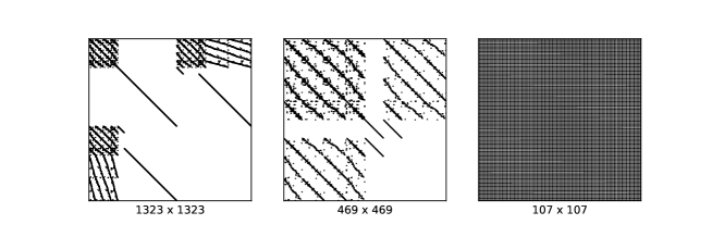
Figure 1: Successive reductions $K_{aug}\to K_{cond}\to K_{red}$ associated with 118ieee.

We establish the last condition to guarantee that we compute a descent direction at each iteration. For any symmetric matrix $M\in\mathbb{R}^{n\times n}$, we note its inertia $\text{I}(M)=(n_{+},n_{-},n_{0})$ as the numbers of positive, negative, and zero eigenvalues.

Theorem 2.3

The step $\bm{p}$ in (6b) is a descent direction if

• $\text{I}(K_{aug})=(n_{x}+n_{u}+m,n_{x}+m,0)$, equivalent to

• $\text{I}(K_{red})=(n_{u}+m,m,0)$, equivalent to

• $\text{I}(K_{cond})=(n_{u},0,0)$ (the condensed matrix $K_{cond}$ is positive definite).

The equivalence of the three conditions can be verified via the Haynsworth inertia additivity formula.

2.2.2 Linearize-then-reduce algorithm (LinRed IPM)

Now that the different reductions have been introduced, we are able to present the linearize-then-reduce (LinRed) algorithm in Algorithm 1, following cervantes2000reduced . The reduction step is in itself an expensive operation, as we will explain in §3.3. The other bottlenecks are the factorization of the dense condensed matrix $K_{cond}$ (which amounts to a Cholesky factorization if the matrix is positive definite) and the factorization of the sparse Jacobian $G_{x}$.

Data: Initial primal variables $(\bm{x}_{0},\bm{u}_{0},\bm{s}_{0})$ and dual variables $(\bm{\lambda}_{0},\bm{y}_{0})$

for $k=0,...$ do

       Evaluate the derivatives $W,G,A$ at $(\bm{x}_{k},\bm{u}_{k})$ ;

       Reduction: Condense the KKT system (6b) in $K_{cond}$ ;

       Control step: Factorize (8a) and solve the system to find $\bm{p}_{u}$ ;

       Dual step: $\bm{p}_{y}=\Sigma_{s}(\hat{A}_{u}\bm{p}_{u}+\hat{\bm{r}}_{3}-\Sigma_{s}^{-1}\hat{\bm{r}}_{2})$;

       Slack step: $\bm{p}_{s}=\Sigma_{s}^{-1}(\bm{p}_{y}-\hat{\bm{r}}_{2})$;

       State step: $\bm{p}_{x}=-G_{x}^{-1}\big{(}\bm{r}_{4}+G_{u}\bm{p}_{u}\big{)}$ ;

       Adjoint step: $\bm{p}_{\lambda}=-G_{x}^{-\top}(\bm{r}_{2}+A_{x}^{\top}\bm{p}_{y}+W_{xu}\bm{p}_{u}+(W_{xx}+\Sigma_{x})\bm{p}_{x})$ ;

       Line search: Update primal-dual direction $(\bm{u}_{k+1},\bm{x}_{k+1},\bm{s}_{k+1},\bm{\lambda}_{k+1},\bm{y}_{k+1})$ using a filter line-search along direction $(\bm{p}_{u},\bm{p}_{x},\bm{p}_{s},\bm{p}_{\lambda},\bm{p}_{y})$;

      

end for

Algorithm 1 Linearize-then-reduce algorithm

2.3 Reduce-then-linearize

We now focus on our second reduction scheme, operating directly at the level of the nonlinear problem (2). This method can be interpreted as an interior-point alternative of the reduced-gradient algorithm of Dommel and Tinney dommel_optimal_1968 and was explored recently in kardos2020reduced .

2.3.1 Nonlinear reduction

Nonlinear projection.

Instead of operating the reduction in the linearized KKT system as in §2.2, Dommel and Tinney’s method uses the implicit function theorem to remove the state variables from the problem.

Theorem 2.4

(Implicit function theorem). Let $g:\mathbb{R}^{n_{x}}\times\mathbb{R}^{n_{u}}\to\mathbb{R}^{n_{x}}$ a continuously differentiable function, and let $(\bm{x},\bm{u})\in\mathbb{R}^{n_{x}}\times\mathbb{R}^{n_{u}}$ such that $g(\bm{x},\bm{u})=0$. If the Jacobian $G_{x}$ is invertible, then there exist an open set $U\subset\mathbb{R}^{n_{u}}$ (with $\bm{u}\in U$) and a unique differentiable function $\underline{x}:U\to\mathbb{R}^{n_{x}}$ such that $g(\underline{x}(\bm{u}),\bm{u})=0$ for all $\bm{u}\in U$.

The implicit function theorem gives, under certain assumptions, the existence of a local differentiable function $\underline{x}:U\to\mathbb{R}^{n_{x}}$ attached to a given control $\bm{u}$. If we assume that on the feasible domain $g(\bm{x},\bm{u})=0$ is solvable and the Jacobian is invertible everywhere, we can derive the reduced-space problem as

$$\min_{\bm{u}}\quad f(\underline{x}(\bm{u}),\bm{u})\quad\text{subject to}\quad\left\{\begin{aligned} \quad&\bm{u}\geq 0\,,\quad\underline{x}(\bm{u})\geq 0\\ &h(\underline{x}(\bm{u}),\bm{u})\leq 0\,.\end{aligned}\right.$$ (11)

In contrast to (2), the problem (11) optimizes only with relation to the control $\bm{u}$, the state being defined implicitly via the local functionals $\underline{x}$. By definition $g(\underline{x}(\bm{u}),\bm{u})=0$, the state equation is automatically satisfied in the reduced-space. However, the reduced-space problem is tied to the assumptions of the implicit function theorem: in some applications, finding a control $\bm{u}$ invertible w.r.t. the state equations (1) can be challenging.

Reduced derivatives.

We define the reduced objective and the reduced constraints as

$$f_{r}(\bm{u}):=f(\underline{x}(\bm{u}),\bm{u})\,,\quad h_{r}(\bm{u}):=\begin{bmatrix}h(\underline{x}(\bm{u}),\bm{u})\\ -\underline{x}(\bm{u})\end{bmatrix}\,,$$ (12)

and we note the reduced Lagrangian $L_{r}(\bm{u},\bm{s};\bm{y}):=f_{r}(\bm{u})+\bm{y}^{\top}(h_{r}(\bm{u})+\bm{s})-\bm{w}^{\top}\bm{u}-\bm{z}^{\top}\bm{s}$. By exploiting the implicit function theorem, we can deduce the derivatives in the reduced-space.

Theorem 2.5

(Reduced derivatives (griewank2008evaluating, , Chapter 15.)) Let $\bm{u}\in\mathbb{R}^{n_{u}}$ such that the conditions of the implicit function theorem hold. Then,

• The functions $f_{r}$ and $h_{r}$ are continuously differentiable, with

  $$\nabla f_{r}(\bm{u})=\bm{g}_{u}-G_{u}^{\top}G_{x}^{-\top}\bm{g}_{x}\,,\quad\hat{A}_{u}=\partial h_{r}(\bm{u})=\begin{bmatrix}A_{u}-A_{x}G_{x}^{-1}G_{u}\\ G_{x}^{-1}G_{u}\end{bmatrix}\;.$$ (13a)

• The Hessian of the reduced Lagrangian $L_{r}$ satisfies

  $$\hat{W}_{uu}=W_{uu}-W_{ux}G_{x}^{-1}G_{u}-G_{u}^{\top}G_{x}^{-\top}W_{xu}+G_{u}^{\top}G_{x}^{-\top}W_{xx}G_{x}^{-1}G_{u}\;.$$ (13b)

Reduced-space KKT system.

The KKT conditions associated with the reduced problem (11) are

$$\nabla_{u}f_{r}+\hat{A}_{u}^{\top}\bm{y}-\bm{w}=0,$$ (14a)

$$\bm{y}-\bm{z}=0,$$ (14b)

$$h_{r}(\bm{u})+\bm{s}=0,$$ (14c)

$$U\bm{w}=0,\;\bm{u},\bm{w}\geq 0,$$ (14d)

$$S\bm{z}=0,\;\bm{s},\bm{z}\geq 0,$$ (14e)

translating, at each iteration of the IPM algorithm, to the following augmented KKT system:

$$\begin{bmatrix}\hat{W}_{uu}+\Sigma_{u}&\phantom{00}0\phantom{00}&\hat{A}_{u}^{\top}\\ 0&\Sigma_{s}&-I\\ \hat{A}_{u}&-I&0\end{bmatrix}\begin{bmatrix}\bm{p}_{u}\\ \bm{p}_{s}\\ \bm{p}_{y}\end{bmatrix}=-\begin{bmatrix}\nabla_{u}L_{r}-\mu U^{-1}\bm{e}_{n_{u}}\\ \bm{y}-\mu S^{-1}\bm{e}_{m}\\ h_{r}(\bm{u})+\bm{s}\end{bmatrix}\,.$$ (15)

We note that we can apply Theorem 2.2 to get a condensed form of the KKT system (15). The KKT system (15) has a structure similar to that of (7a) but with minor differences. (i) The state $\bm{x}$ and the adjoint $\bm{\lambda}$ are updated independently of (15), respectively by solving the state equation (1) and by solving a linear system. (ii) The bounds $\bm{x}\geq 0$ are incorporated inside the function $h_{r}$, whereas (7a) handles them explicitly in the KKT system (leading to an additional term $\Sigma_{x}$ in the reduced Hessian $\hat{W}_{uu}$). (iii) The right-hand side in (7a) incorporates additional second-order terms that do not appear in (15). Indeed, as here with $\bm{r}_{4}=g(\bm{x},\bm{u})=0$, all the terms associated with $\bm{r}_{4}$ disappeared in the right-hand side of (15), including the second-order terms.

2.3.2 Reduce-then-linearize algorithm (RedLin IPM)

At each iteration $k$, the reduce-then-linearize (RedLin) algorithm proceeds in two steps. First, given a new control $\bm{u}_{k}$, the algorithm finds a state $\bm{x}_{k}$ satisfying $g(\bm{x}_{k},\bm{u}_{k})=0$ by using a nonlinear solver. Then, once $\bm{x}_{k}$ has been computed, the reduced derivatives are updated, and the condensed form of the system (15) is solved to compute the next iterate. This process is summarized in Algorithm 2. We note that compared with Algorithm 1, the state step and the adjoint step are computed before solving the KKT system, since we first have to solve (1). In addition, the algorithm gives no guarantee that at iteration $k$ there exists a state $\bm{x}_{k}$ such that $g(\bm{x}_{k},\bm{u}_{k})=0$, which can be problematic on certain applications. On the other hand, even if interrupted early, the algorithm produces state variables that are feasible for the state equation (1), which may be important in real-time applications.

Data: Initial primal variable $(\bm{u}_{0},\bm{s}_{0})$ and dual variable $(\bm{y}_{0})$

for $k=0,...$ do

       Projection: Find $\bm{x}_{k}$ satisfying $g(\bm{x}_{k},\bm{u}_{k})=0$ ;

       Adjoint step: Solve $\bm{\lambda}=-G_{x}^{-\top}\nabla_{x}L$ ;

       Reduction: Condense the KKT system (15) in $K_{cond}$ ;

       Control step: Factorize $K_{cond}$ and solve the system to find $\bm{p}_{u}$ ;

       Dual step: $\bm{p}_{y}=\Sigma_{s}(\hat{A}_{u}\bm{p}_{u}+\hat{\bm{r}}_{3}-\Sigma_{s}^{-1}\hat{\bm{r}}_{2})$;

       Slack step: $\bm{p}_{s}=\Sigma_{s}^{-1}(\bm{p}_{y}-\hat{\bm{r}}_{2})$;

       Line search: Update primal-dual direction $(\bm{u}_{k+1},\bm{s}_{k+1},\bm{y}_{k+1})$ using a filter line-search along direction $(\bm{p}_{u},\bm{p}_{s},\bm{p}_{y})$;

      

end for

Algorithm 2 Reduce-then-linearize algorithm

3 Implementation of reduced IPM on GPU

In this section we present a GPU implementation of the reduced-space algorithm. To avoid expensive data transfers between the host and the device, we have designed our implementation to run as much as possible on the GPU, comprising (i) the evaluation of the callbacks, (ii) the reduction algorithm, and (iii) the dense factorization of the condensed KKT system. At the end, only the interior-point routines (line search, second-order correction, etc.) run on the host. In particular, our method does not require transferring dense matrices between device and host, and most of the operations performed on the host are simple scalar operations.

3.1 GPU operations

The key idea is to exploit efficient computation kernels on the GPU to implement the reduction algorithm. To the extent possible, we avoid writing custom kernels and rely instead on the BLAS and LAPACK operations, as provided by the vendor library (CUDA in our case).

We list below the specific kernels we are targeting (Sp stands for sparse, Dn for dense).

• SpMV/SpMM (sparse matrix-vector product/sparse matrix-dense matrix product). On the GPU, sparse matrices are stored in condensed sparse row (CSR) format, allowing the sparse multiplication kernels to be run fully in parallel.

• SpSV/SpSM (sparse triangular solve). Once an LU factorization is computed (for instance with SpRF), a sparse matrix $A$ is decomposed as $PAQ=LU$, with $P$ and $Q$ two permutation matrices, $L$ and $U$ being respectively a lower and an upper triangular matrix. The routine SpSV solves the triangular systems $L^{-1}\bm{b}$ and $U^{-1}\bm{b}$ efficiently. The extension to multiple right-hand sides is directly provided by the SpSM kernel.

• SpRF (sparse LU refactorization). GPUs are notoriously inefficient at factorizing a sparse matrix $M$. If the sparse matrix $M$ has always the same sparsity pattern, however, we can compute the initial factorization on the CPU and move the factors back to the GPU. Then, if the nonzero coefficients of the matrix changes, the matrix can be refactorized entirely on the GPU, by updating directly the $L$ and $U$ factors.

3.2 Porting the callbacks to the GPU

In nonlinear programming, the evaluation of the callbacks is often one of the most time-consuming parts, and the OPF problem is not immune to this issue. Most of the time, the derivatives of the OPF model are provided explicitly zimmerman2010matpower , evaluated by using automatic differentiation dunning2017jump ; fourer1990modeling or symbolic differentiation hijazi2018gravity . Here we have chosen to stick with automatic differentiation. We have streamlined on the GPU the evaluation of the objective and of the constraints by adopting the vectorized model proposed in lee2020feasible . This model factorizes all the nonlinearities inside a single basis function, which can be evaluated in parallel inside a single GPU kernel. In addition, we have designed our implementation to be differentiable with ForwardDiff.jl revels2016forward . In total, each iteration of the reduced IPM algorithm requires one evaluation of the objective’s gradient (=one reverse pass), one evaluation of the Jacobian of the constraints (=one forward pass), and one evaluation of the Hessian of the Lagrangian (=one forward-over-reverse pass).

The OPF comes with two decisive advantages. (i) Its structure is supersparse, rendering all the SpMV operations efficient (we have at most a dozen of nonzeroes on each rows of the sparse matrices). (ii) The sparsity of the Jacobian $G_{x}$ is fixed (it is associated with the structure of the power network), allowing for efficient refactorization with SpRF.

3.3 Porting the reduction algorithm to the GPU

Once the derivatives are evaluated in the full space, it remains to build the condensed KKT system (8a). The algorithm has to be repeated at each iteration of the IPM algorithm, and its performance is critical. If we denote $K=W+A^{\top}\Sigma_{s}A$, then we note that

$$\hat{W}_{uu}+\hat{A}_{u}^{\top}\Sigma_{s}\hat{A}_{u}=\begin{bmatrix}I\\ -G_{x}^{-1}G_{u}\end{bmatrix}^{\top}\begin{bmatrix}K_{uu}&K_{ux}\\ K_{xu}&K_{xx}\end{bmatrix}\begin{bmatrix}I\\ -G_{x}^{-1}G_{u}\end{bmatrix}\equiv\hat{K}_{uu}\;.$$ (16)

Evaluating (16) requires three different operations: (i) factorizing the Jacobian $G_{x}$ (SpRF), (ii) triangular solves $G_{x}^{-1}b$ (SpSV/SpSM), and (iii) sparse-matrix matrix multiplications with $K$ (SpMM). The order in which the operations are performed is important, affecting the complexity of the reduction algorithm.

The naive idea is to evaluate first the sensitivity matrix $S=-G_{x}^{-1}G_{u}$, in order to reduce the total number of linear solves to $n_{u}$. However, the matrix $S$ is dense, with size $n_{x}\times n_{u}$, and the cross-product $S^{\top}K_{xx}S$ requires storing another intermediate dense matrix with size $n_{x}\times n_{u}$ to evaluate the dense product $S^{\top}(K_{xx}S)$ (which is itself slow when $n_{x}$ is large). This renders the algorithm not tractable on the largest instances.

Hence, we avoid computing the full sensitivity matrix $S$ and rely instead on a batched variant of the adjoint-adjoint algorithm pacaud2022batched . First, we compute an LU factorization of $G_{x}$, as $PG_{x}Q=L\,U$, with $P$ and $Q$ two permutation matrices and $L$ and $U$ being respectively a lower and an upper triangular matrix (using SpRF, the factorization can be updated entirely on the GPU if the sparsity pattern of $G_{x}$ is the same along the iterations). Once the factorization is computed, solving the linear solve $G_{x}^{-1}\bm{b}$ translates to 2 SpMV and 2 SpSV routines, as $G_{x}^{-1}\bm{b}=QU^{-1}L^{-1}P\bm{b}$.

Second, we build the sparse matrix $K\in\mathbb{R}^{(n_{x}+n_{u})\times(n_{x}+n_{u})}$ (nontrivial but doable in one sparse addition and one sparse-sparse multiplication SpGEMM). Then, for a batch size $N$, the algorithm takes as input a dense matrix $V\in\mathbb{R}^{n_{u}\times N}$ and evaluates the Hessian-matrix product $\hat{K}_{uu}V$ with three successive operations.

1. Solve $Z=-G_{x}^{-1}(G_{u}\,V)$. (3 SpMM, 2 SpSM)

2. Evaluate $\begin{bmatrix}H_{u}\\ H_{x}\end{bmatrix}=\begin{bmatrix}K_{uu}&K_{ux}\\ K_{xu}&K_{xx}\end{bmatrix}\begin{bmatrix}V\\ Z\end{bmatrix}$. (1 SpMM)

3. Solve $\Psi=G_{x}^{-\top}H_{x}$ and get $\hat{K}_{uu}=H_{u}-G_{u}\Psi$. (3 SpMM, 2 SpSM)

One Hessian-matrix product $\hat{K}_{uu}V$ requires $2N$ linear solves (streamlined in four SpSM operations), giving a total of 7 SpMM and 4 SpSM operations. Evaluating $\hat{K}_{uu}V$ requires $3\times n_{x}\times N$ storage for the two intermediates $Z,\Psi\in\mathbb{R}^{n_{x}\times N}$, as well as an additional buffer to store the permuted matrix in the LU triangular solves. Overall, the evaluation of the full reduced matrix $\hat{K}_{uu}$ requires $\text{div}(n_{u},N)+1$ Hessian-matrix products, giving a complexity proportional to the number of controls $n_{u}$.

4 Numerical results

In this section we assess the performance of the reduced IPM algorithm on the various OPF instances presented in §4.1. First, we evaluate in §4.2 the scalability of the GPU-accelerated reduction algorithm initially presented in §3.3. Next, we present in §4.3 a detailed assessment of the reduced IPM algorithm on the GPU, by comparing its performance with that of a state-of-the-art full-space IPM working on the CPU. Then, we present in §4.4 a comparison of our two reduced-space algorithms: linearize-then-reduce (LinRed) and reduce-then-linearize (RedLin).

4.1 Benchmark instances

We benchmark the reduced IPM algorithm on the OPF problem. We select in Table 1 a subset of the MATPOWER cases provided in zimmerman2010matpower , whose size varies from medium to large scale. In addition, we add three cases from the PGLIB benchmark babaeinejadsarookolaee2019power with fewer degrees of freedom (as indicated by the ratio $\frac{n_{u}}{n_{x}+n_{u}}$). Our algorithms have been implemented in Julia for portability. All the benchmarks presented have been generated on our workstation, equipped with an NVIDIA V100 GPU and using CUDA 11.4. The code, open source, is available on https://github.com/exanauts/Argos.jl/.

Case	$n_{b}$	$n_{\ell}$	$n_{g}$	$n_{x}$	$n_{u}$	$n_{u}/(n_{x}+n_{u})$
118ieee	118	186	54	181	107	0.37
300ieee	300	411	69	530	137	0.21
ACTIVSg500	500	597	56	943	111	0.11
1354pegase	1,354	1,991	260	2,447	519	0.17
ACTIVSg2000	2,000	3,206	432	3,607	783	0.18
2869pegase	2,869	4,582	510	5,227	1,019	0.16
9241pegase	9,241	16,049	1,445	17,036	2,889	0.14
ACTIVSg10k	10,000	12,706	1,937	18,544	2,909	0.14
13659pegase	13,659	20,467	4,092	23,225	8,183	0.26
ACTIVSg25k	25,000	32,230	3,779	47,246	5,505	0.10
ACTIVSg70k	70,000	88,207	8,107	134,104	11,789	0.08
9591_goc	9,591	15,915	365	19,013	335	0.02
10480_goc	10,480	18,559	777	20,620	677	0.03
19402_goc	19,402	34,704	971	38,418	769	0.02

Table 1: Case instances obtained from MATPOWER

4.2 How far can we parallelize the reduction algorithm on the GPU?

We first benchmark the reduction algorithm on the instances in Table 1. For SpRF, the reduction algorithm uses the library cusolverRF (with an initial factorization computed by KLU), the kernels SpSM and SpMM being provided by cuSPARSE. We show in Figure 2 (a) that cusolverRF is able to refactorize efficiently the Jacobian $G_{x}$ on the GPU (its sparsity pattern is constant, and given by the structure of the underlying network). In Figure 2 (b), we depict the performance of the reduction algorithm against the batch size $N$. We observe that the greater the size $N$, the better is the performance, until we reach the scalability limit of the GPU. For instance, on ACTIVSg70k we reach the limit when $N=512$, meaning we cannot parallelize the algorithm further on the GPU. This limits the performance of the reduction since $\text{div}(11\,789,512)+1=24$ batched Hessian-matrix products remain to be computed to evaluate the reduced Hessian of ACTIVSg70k. We note that, overall, it makes no sense to use a batch size greater than $N=256$.

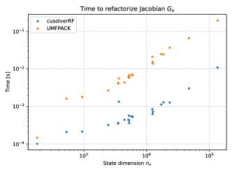
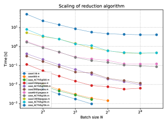
(a)	(b)

Figure 2: Performance of the reduction algorithm: (a) time spent refactorizing the Jacobian $G_{x}$ in cusolverRF and in UMFPACK; (b) performance of the reduction algorithm against the batch size $N$.

4.3 Linearize-then-reduce or full-space interior-point?

We have implemented the linearize-then-reduce (LinRed) inside the MadNLP solver shin2021graph . As a reference, we benchmark our code against Knitro 13.0 waltz2006interior and MATPOWER zimmerman2010matpower . We note that the performance is consistent with that reported in the recent benchmark kardos2018complete . Our implementation uses the vectorized OPF model introduced in §3.2, which runs entirely on the GPU (including the evaluation of the derivatives). MadNLP runs in inertia-based mode: Theorem 2.3 states that the inertia is correct if and only if the reduced matrix $K_{cond}$ is positive-definite. This fact is exploited in LinRed. At each iteration the algorithm factorizes the matrix $K_{cond}$ with the dense Cholesky solver shipped with cusolver; if the factorization fails, we apply a primal-dual regularization to $K_{cond}$ until it becomes positive-definite. In addition, we use the reduction algorithm presented in §3.3 with a batch size $N=256$. We compare LinRed with a hybrid full-space IPM algorithm using also the GPU-accelerated OPF model but solving the original augmented system (6b) on the CPU with the linear solver MA27 (hence combining the best of both worlds). The hybrid full-space IPM and LinRed both use the same model and the same derivatives and are equivalent in exact arithmetic unless we run into a feasibility restoration phase. In that edge case, the algebra of LinRed can be adapted but no longer follows the workflow we presented above. In that circumstance, LinRed applies the dual regularization only on the inequality constraints, to fit the linear algebra framework we introduced in §2.2.

Concerning scaling, MadNLP uses the same approach as Ipopt, based on the norm of the first-order derivatives wachter2006implementation . The initial primal variables $(\bm{x}_{0},\bm{u}_{0})$ are specified inside the MATPOWER file, and the initial dual variables are set to zero: $\bm{y}_{0}=0$. The algorithm stops when the primal and dual infeasibilities are below $10^{-8}$. The results of the benchmark are presented in Table 2. Here, the dagger sign $\dagger$ indicates that the IPM algorithm runs into a feasibility restoration: this is the case both for ACTIVSg10k and for ACTIVSg70k (even Knitro struggles on these two instances, with numerous conjugate gradient iterations performed).

	Knitro		Hybrid full-space IPM			LinRed
Case	#it	Time (s)	#it	Time (s)	MA27 (s)	#it	Time (s)	Chol. (s)	Reduction (s)
ieee118	10	0.06	16	0.17	0.01	16	0.26	0.01	0.02
ieee300	10	0.12	22	0.28	0.06	22	0.42	0.02	0.03
ACTIVSg500	20	0.51	24	0.29	0.06	24	0.45	0.02	0.03
1354pegase	22	1.17	40	0.85	0.35	40	1.16	0.09	0.29
ACTIVSg2000	18	1.62	43	1.95	1.42	43	2.40	0.24	0.65
2869pegase	22	2.11	50	2.03	1.18	50	2.69	0.20	0.97
9241pegase	102	31.7	69	10.65	6.14	69	23.72	1.17	16.23
ACTIVSg10k	130	39.3	76${}^{\dagger}$	7.9	5.66	88${}^{\dagger}$	21.9	1.5	14.7
13659pegase	120	116.0	346	98.31	67.13	145	242.69	19.23	202.89
ACTIVSg25k	47	36.1	86	24.70	16.86	86	84.96	4.27	68.11
ACTIVSg70k	101	242.0	90${}^{\dagger}$	89.8	65.7	85${}^{\dagger}$	658.2	21.5	606.5
9591goc	37	22.5	43	11.66	10.38	43	7.69	2.13	1.61
10480goc	40	25.7	50	13.98	11.95	50	11.46	3.93	3.34
19402goc	45	66.5	47	30.75	26.83	47	19.52	4.86	7.24

Table 2: Benchmarking LinRed with Full-space IPM

We make the following observations. (i) Hybrid full-space IPM is slightly faster than Knitro, but only because it evaluates the derivatives on the GPU. (ii) LinRed is able to solve all the instances, including ACTIVSg70k. (iii) As expected, we get the same number of iterations between Full-space IPM and LinRed except on 13659pegase. This case is indeed ill-conditioned, and the convergence is sensitive to the linear solver employed (even MA27 and MA57 give different results on this case). (iv) Despite the good performance of the Cholesky factorization, LinRed is negatively impacted by the scalability of the reduction algorithm: the larger the relative number of controls with respect to the total number of variables, the less competitive is the reduction. On the largest instances, LinRed beats Full-space IPM only on the three goc instances, which have fewer degrees of freedom (see Table 1).

4.4 Linearize-then-reduce or reduce-then-linearize?

Now we benchmark LinRed with its feasible variant, RedLin. In contrast to LinRed, RedLin follows a feasible path w.r.t. the state equations (1): the algorithm can be stopped at any time and return a feasible point, an advantageous feature if the resolution is time-constrained. LinRed uses the same setting as before, and RedLin is also using the MadNLP solver, using the reduced derivatives defined in (13). RedLin solves the state equations (1) (the power flow balance equations) at each iteration with a Newton–Raphson algorithm, with a tolerance of $10^{-10}$. The algorithm has two drawbacks: (i) this approach requires evaluating the reduced Jacobian $\hat{A}_{u}$, with size $m\times n_{u}$, and (ii) the default scaling computed by MadNLP depends on $G_{x}^{-1}$, rendering the scaling inappropriate if $G_{x}$ has a poor conditioning. To ensure that the comparison is fair, we have modified our implementation so that RedLin uses the same scaling as LinRed. The results are presented in Figure 3 (the time spent in the reduction is omitted since it is the same as in LinRed).

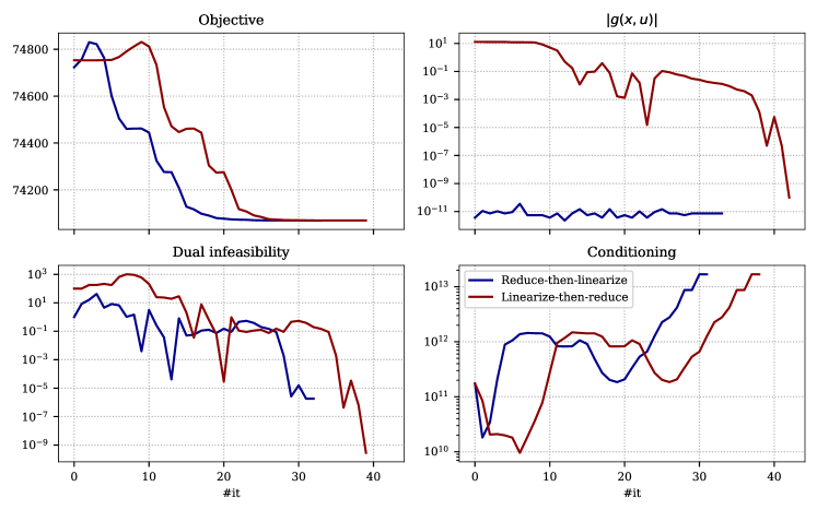
(a) Convergence of RedLin (blue) and LinRed (red) on 1354pegase.

Case	#it	Time (s)	Chol. (s)	PF (s)
case118	16	0.40	0.01	0.13
case300	24	0.55	0.02	0.20
ACTIVSg500	22	0.58	0.01	0.23
1354pegase	32	1.34	0.05	0.35
ACTIVSg2000	33	2.25	0.07	0.65
2869pegase	34	2.62	0.08	0.67
9241pegase	48	28.30	0.78	3.05
ACTIVSg10k	140	90.53	3.60	5.51
13659pegase	167	944.04	33.19	15.78
ACTIVSg25k	52	156.17	1.79	5.36
ACTIVSg70k	-	-	-	-

(b) Performance of RedLin.

Figure 3: Benchmarking LinRed with RedLin.

Comparing with Table 2, we make the following observations. (i) RedLin is able to solve instances with up to 25,000 buses, which, to the best of our knowledge, is a net improvement compared with previous attempts to solve the OPF in the reduced-space kardos2020reduced ; pacaud2021feasible . (ii) On the largest instances, RedLin is penalized compared with LinRed, since it has to deal with the reduced Jacobian $\hat{A}_{u}$. For that reason, RedLin breaks on ACTIVSg70k, since we are running out of memory. (iii) From case118 to 9241pegase, RedLin converges in fewer iterations than does LinRed. (iv) The time to solve the power flow (column PF) is a fraction of the time spent in the reduction algorithm. (v) On ACTIVSg10k, RedLin does not run into the feasibility restoration we encountered in LinRed: on this difficult instance, the convergence of RedLin is smoother, even if it requires more iterations. (vi) the Newton–Raphson is not guaranteed to converge, but empirically we find this is not an issue when a second-order method is employed.

In Figure 3(a) we compare the convergence of the two algorithms on 1354pegase. We observe that RedLin converges faster than LinRed, the latter satisfying the power flow equations only at the final iterations. Interestingly, the conditioning of the KKT matrix $K_{cond}$ does not blow up at the final iterations and remains below $10^{13}$, a reasonable value for an interior-point algorithm.

5 Conclusion

This paper has presented an efficient implementation of the IPM on GPU architectures, based on a Schur reduction of the underlying KKT system. We have derived two practical algorithms, linearize-then-reduce and reduce-then-linearize, adapted their workflows to be efficient when the vast majority of their computation is run on the GPU, and detailed their respective performance on different large-scale OPF instances. We also discussed the benefits of a hybrid full space IPM solver — computing the derivatives on the GPU and the linear algebra on the CPU — and demonstrated that this approach generally outperforms Knitro, running exclusively on the CPU. The relative performance of the reduced-space algorithms is highly dependent on the ratio of controls with respect to the total number of variables. Their performance lags behind both Knitro and the hybrid full space solver when the problem has many control variables (as it is the case on the MATPOWER benchmark) but is significantly ahead – up to a factor of 3 – when the problem has a relatively lower number of control variables. Moreover, the reduce-then-linearize algorithm has the added benefit of producing a feasible solution to the power flow equations at any iteration, which makes it a great candidate for real time applications. To improve the performance of reduction algorithms, we believe the most important item is to alleviate the dependence on the number of control variables. We plan to explore a way to accelerate the reduction by exploiting the exponentially decaying structure of the reduced Hessian shin2021exponential .

Acknowledgments

We thank Juraj Kardoš for reviving the interest in reduced-space methods and Kasia Świrydowicz for pointing us to the cusolverRF library. This research was supported by the Exascale Computing Project (17-SC-20-SC), a joint project of the U.S. Department of Energy’s Office of Science and National Nuclear Security Administration, responsible for delivering a capable exascale ecosystem, including software, applications, and hardware technology, to support the nation’s exascale computing imperative. The material is based upon work supported in part by the U.S. Department of Energy, Office of Science, under contract DE-AC02-06CH11357.

The submitted manuscript has been created by UChicago Argonne, LLC, Operator of Argonne National Laboratory (“Argonne”). Argonne, a U.S. Department of Energy Office of Science laboratory, is operated under Contract No. DE-AC02-06CH11357. The U.S. Government retains for itself, and others acting on its behalf, a paid-up nonexclusive, irrevocable worldwide license in said article to reproduce, prepare derivative works, distribute copies to the public, and perform publicly and display publicly, by or on behalf of the Government. The Department of Energy will provide public access to these results of federally sponsored research in accordance with the DOE Public Access Plan. http://energy.gov/downloads/doe-public-access-plan.

References

- (1) J. Abadie and J. Carpentier, Generalization of the Wolfe reduced gradient method to the case of nonlinear constraints, 1969.
- (2) S. Babaeinejadsarookolaee, A. Birchfield, R. D. Christie, C. Coffrin, C. DeMarco, R. Diao, M. Ferris, S. Fliscounakis, S. Greene, R. Huang, et al., The power grid library for benchmarking AC optimal power flow algorithms, arXiv preprint arXiv:1908.02788, (2019).
- (3) L. T. Biegler, J. Nocedal, and C. Schmid, A reduced Hessian method for large-scale constrained optimization, SIAM Journal on Optimization, 5 (1995), pp. 314–347.
- (4) G. Biros and O. Ghattas, Parallel Lagrange–Newton–Krylov–Schur methods for PDE-constrained optimization: Part I – The Krylov–Schur Solver, SIAM Journal on Scientific Computing, 27 (2005), pp. 687–713.
- (5) R. Burchett, H. Happ, and D. Vierath, Quadratically convergent optimal power flow, IEEE Transactions on Power Apparatus and Systems, (1984), pp. 3267–3275.
- (6) M. B. Cain, R. P. O’neill, A. Castillo, et al., History of optimal power flow and formulations, Federal Energy Regulatory Commission, 1 (2012), pp. 1–36.
- (7) Y. Cao, A. Seth, and C. D. Laird, An augmented Lagrangian interior-point approach for large-scale NLP problems on graphics processing units, Computers & Chemical Engineering, 85 (2016), pp. 76–83.
- (8) A. M. Cervantes, A. Wächter, R. H. Tütüncü, and L. T. Biegler, A reduced space interior point strategy for optimization of differential algebraic systems, Computers & Chemical Engineering, 24 (2000), pp. 39–51.
- (9) T. F. Coleman and A. R. Conn, Nonlinear programming via an exact penalty function: Asymptotic analysis, Mathematical Programming, 24 (1982), pp. 123–136.
- (10) H. Dommel and W. Tinney, Optimal power flow solutions, IEEE Transactions on Power Apparatus and Systems, PAS-87 (1968), pp. 1866–1876.
- (11) I. S. Duff, MA57—a code for the solution of sparse symmetric definite and indefinite systems, ACM Transactions on Mathematical Software (TOMS), 30 (2004), pp. 118–144.
- (12) I. Dunning, J. Huchette, and M. Lubin, JuMP: A modeling language for mathematical optimization, SIAM review, 59 (2017), pp. 295–320.
- (13) R. Fletcher, Practical methods of optimization, John Wiley & Sons, 2013.
- (14) R. Fourer, D. M. Gay, and B. W. Kernighan, A modeling language for mathematical programming, Management Science, 36 (1990), pp. 519–554.
- (15) S. Frank, I. Steponavice, and S. Rebennack, Optimal power flow: a bibliographic survey I, Energy systems, 3 (2012), pp. 221–258.
- (16) D. Gabay, Minimizing a differentiable function over a differential manifold, Journal of Optimization Theory and Applications, 37 (1982), pp. 177–219.
- (17) A. Griewank and A. Walther, Evaluating derivatives: principles and techniques of algorithmic differentiation, SIAM, 2008.
- (18) C. B. Gurwitz and M. L. Overton, Sequential quadratic programming methods based on approximating a projected Hessian matrix, SIAM Journal on Scientific and Statistical Computing, 10 (1989), pp. 631–653.
- (19) H. Hijazi, G. Wang, and C. Coffrin, Gravity: A mathematical modeling language for optimization and machine learning, Machine Learning Open Source Software Workshop at NeurIPS 2018, (2018). Available at www.gravityopt.com.
- (20) Q. Jiang and G. Geng, A reduced-space interior point method for transient stability constrained optimal power flow, IEEE Transactions on Power Systems, 25 (2010), pp. 1232–1240.
- (21) J. Kardos, D. Kourounis, and O. Schenk, Reduced-space interior point methods in power grid problems, arXiv preprint arXiv:2001.10815, (2020).
- (22) J. Kardos, D. Kourounis, O. Schenk, and R. Zimmerman, Complete results for a numerical evaluation of interior point solvers for large-scale optimal power flow problems, arXiv preprint arXiv:1807.03964, (2018).
- (23) Y. Kim, F. Pacaud, K. Kim, and M. Anitescu, Leveraging GPU batching for scalable nonlinear programming through massive Lagrangian decomposition, arXiv preprint arXiv:2106.14995, (2021).
- (24) D. Lee, K. Turitsyn, D. K. Molzahn, and L. A. Roald, Feasible path identification in optimal power flow with sequential convex restriction, IEEE Transactions on Power Systems, 35 (2020), pp. 3648–3659.
- (25) J. Nocedal and M. L. Overton, Projected Hessian updating algorithms for nonlinearly constrained optimization, SIAM Journal on Numerical Analysis, 22 (1985), pp. 821–850.
- (26) J. Nocedal and S. J. Wright, Numerical optimization, Springer series in operations research, Springer, New York, 2nd ed ed., 2006. OCLC: ocm68629100.
- (27) F. Pacaud, D. A. Maldonado, S. Shin, M. Schanen, and M. Anitescu, A feasible reduced space method for real-time optimal power flow, arXiv preprint arXiv:2110.02590, (2021).
- (28) F. Pacaud, M. Schanen, D. A. Maldonado, A. Montoison, V. Churavy, J. Samaroo, and M. Anitescu, Batched second-order adjoint sensitivity for reduced space methods, arXiv preprint arXiv:2201.00241, (2022).
- (29) J. Revels, M. Lubin, and T. Papamarkou, Forward-mode automatic differentiation in Julia, arXiv preprint arXiv:1607.07892, (2016).
- (30) J. B. Rosen, The gradient projection method for nonlinear programming: Part II – Nonlinear constraints, Journal of the Society for Industrial and Applied Mathematics, 9 (1961), pp. 514–532.
- (31) R. Sargent et al., Reduced-gradient and projection methods for nonlinear programming, Numerical Methods for Constrained Optimization, 149 (1974).
- (32) O. Schenk and K. Gärtner, Solving unsymmetric sparse systems of linear equations with PARDISO, Future Generation Computer Systems, 20 (2004), pp. 475–487.
- (33) M. Schubiger, G. Banjac, and J. Lygeros, GPU acceleration of ADMM for large-scale quadratic programming, Journal of Parallel and Distributed Computing, 144 (2020), pp. 55–67.
- (34) S. Shin, M. Anitescu, and V. M. Zavala, Exponential decay of sensitivity in graph-structured nonlinear programs, arXiv preprint arXiv:2101.03067, (2021).
- (35) S. Shin, C. Coffrin, K. Sundar, and V. M. Zavala, Graph-based modeling and decomposition of energy infrastructures, IFAC-PapersOnLine, 54 (2021), pp. 693–698.
- (36) K. Świrydowicz, E. Darve, W. Jones, J. Maack, S. Regev, M. A. Saunders, S. J. Thomas, and S. Peleš, Linear solvers for power grid optimization problems: a review of GPU-accelerated linear solvers, Parallel Computing, (2021), p. 102870.
- (37) B. Tasseff, C. Coffrin, A. Wächter, and C. Laird, Exploring benefits of linear solver parallelism on modern nonlinear optimization applications, arXiv preprint arXiv:1909.08104, (2019).
- (38) A. Wächter and L. T. Biegler, On the implementation of an interior-point filter line-search algorithm for large-scale nonlinear programming, Mathematical Programming, 106 (2006), pp. 25–57.
- (39) R. A. Waltz, J. L. Morales, J. Nocedal, and D. Orban, An interior algorithm for nonlinear optimization that combines line search and trust region steps, Mathematical Programming, 107 (2006), pp. 391–408.
- (40) R. D. Zimmerman, C. E. Murillo-Sánchez, and R. J. Thomas, MATPOWER: Steady-state operations, planning, and analysis tools for power systems research and education, IEEE Transactions on Power Systems, 26 (2010), pp. 12–19.