Nonstationary Nearest Neighbor Gaussian Process: hierarchical model architecture and MCMC sampling

Abstract

Nonstationary spatial modeling presents several challenges including, but not limited to, computational cost, the complexity and lack of interpretation of multi-layered hierarchical models, and the challenges in model assessment and selection. This manuscript develops a class of nonstationary Nearest Neighbor Gaussian Process (NNGP) models. NNGPs are a good starting point to address the problem of the computational cost because of their accuracy and affordability. We study the behavior of NNGPs that use a nonstationary covariance function, exploring their properties and the impact of ordering on the effective covariance induced by NNGPs. To simplify spatial data analysis and model selection, we introduce an interpretable hierarchical model architecture, where, in particular, we make parameter interpretation and model selection easier by integrating stationary range, nonstationary range with circular parameters, and nonstationary range with elliptic parameters within a coherent probabilistic structure. Given the NNGP approximation and the model framework, we propose a MCMC implementation based on Hybrid Monte-Carlo and nested interweaving of parametrizations. We carry out experiments on synthetic data sets to explore model selection and parameter identifiability and assess inferential improvements accrued from the nonstationary model. Finally, we use those guidelines to analyze a data set of lead contamination in the United States of America.

Keywords: Bayesian hierarchical models; Hybrid Monte-Carlo; Interweaving; Nearest-Neighbor Gaussian processes; Nonstationary spatial modeling.

1 Introduction

Bayesian hierarchical models for analyzing spatially and temporally oriented data are widely employed in scientific and technological applications in the physical, environmental and health sciences (Cressie and Wikle,, 2015; Banerjee et al.,, 2014; Gelfand et al.,, 2019). Such models are constructed by embedding a spatial process within a hierarchical structure,

$$[\mbox{data}\,|\,\mbox{process},\;\mbox{parameters}]\times[\mbox{process}\,|\,\mbox{parameters}]\times[\mbox{parameters}]\;,$$ (1)

which specifies the joint probability law of the data, an underlying spatial process and the parameters. The process in (1) is a crucial inferential component that introduces spatial and/or temporal dependence, allows us to infer about the underlying data generating mechanism and carry out predictions over entire spatial-temporal domains.

Point-referenced spatial data, which is our focus here, refer to measurements over a set of locations with fixed coordinates. These measurements are assumed to arise as a partial realization of a spatial process over the finite set of locations. A stationary Gaussian process is a conspicuous specification in spatial process models. Stationarity imposes a simplifying assumption on the dependence structure of the process such as the association between measurements at any two points being a function of the separation between the two points. While this assumption is unlikely to hold in most scientific applications, stationary Gaussian process models are easier to compute. Also, they can effectively capture spatial variation and substantially improve predictive inference that are widely sought in environmental data sets. The aforementioned references provide several examples of stationary Gaussian process models and their effectiveness.

Nonstationary spatial models relax assumptions of stationarity and can deliver wide-ranging benefits to inference. For example, when variability in the data is a complex function of space composed of multiple locally varying processes, the customary stationary covariance kernels may be inadequate. Here, richer and more informative covariance structures in nonstationary processes, while adding complexity, may be more desirable by improving smoothing, goodness of fit and predictive inference. Nonstationary spatial models have been addressed by a number of authors (Higdon,, 1998; Fuentes,, 2002; Paciorek,, 2003; Banerjee et al.,, 2008; Cressie and Johannesson,, 2008; Yang and Bradley,, 2021; Risser and Calder,, 2015; Risser,, 2016; Fuglstad et al., 2015a, ; Gelfand et al.,, 2010, chapter 9)

The richness sought in nonstationary models have been exemplified in a number of the above references. Paciorek, (2003) and Kleiber and Nychka, (2012) introduce nonstationarity by allowing the parameters of the Matérn class to vary with location, yielding local variances, local ranges and local geometric anisotropies. Such ideas have been extended and further developed in a number of different directions but have not been devised for implementation on massive data sets in the order of $10^{5}+$. For example, recent works have addressed data sets in the order of hundreds (Risser and Calder,, 2015; Ingebrigtsen et al.,, 2015; Heinonen et al.,, 2016) or thousands (Fuglstad et al., 2015a, ) of locations, but this is modest with respect to the size of commonly encountered spatial data (see the examples in Datta et al.,, 2016; Heaton et al.,, 2019; Katzfuss and Guinness,, 2021). A second challenge with nonstationary models is overparametrization arising from complex space-varying covariance kernels. This can lead to weakly identifiable models that are challenging to interpret and difficult to estimate. This also complicates model evaluation and selection as inference is very sensitive to the specifications of the model.

We devise a new class of nonstationary spatial models for massive data sets that build upon Bayesian hierarchical models based on directed acyclic graphs (DAGs) such as the Nearest Neighbor Gaussian Process models (Datta et al.,, 2016) and, more generally, the family of Vecchia approximations (Katzfuss and Guinness,, 2021) to nonstationarity, which allow us to exploit their attractive computational and inferential properties (Katzfuss and Guinness,, 2021; Finley et al.,, 2019; Guinness,, 2018). The underlying idea is to endow the nonstationary process model from Paciorek, (2003) with NNGP specifications on the processes defining the parameters. Our approach relies upon matrix logarithms to specify processes for the elliptic covariance parameters of Paciorek, (2003). The resulting parametrization is sparser than Paciorek, (2003) or Risser and Calder, (2015) and is a natural extension of the usual logarithmic prior for positive parameters such as the marginal variance, the noise variance, and the range when it is not elliptic. We embed this nonstationary NNGP in a coherent and interpretable hierarchical Bayesian model framework as in Heinonen et al., (2016), but differ in our focus on modeling large spatial data sets.

A key challenge is learning about the nonstationary covariance processes. We pursue a Hamiltonian Monte Carlo (HMC) algorithm adapted from Heinonen et al., (2016). Here, we draw distinctions from Heinonen et al., (2016) who used a full GP and classical matrix calculus that are impracticable for handling massive data sets and, specifically, for NNGP or other DAG-based models. We devise such algorithms specifically for NNGP models to achieve computational efficiency. We also differ from Heinonen et al., (2016) in that we pursue hierarchical latent process modeling. Estimating the latent field (Finley et al.,, 2019) allows us to model non-Gaussian responses as well. In order to obtain an efficient algorithm, we hybridize the approach of Heinonen et al., (2016) with interweaving strategies of Yu and Meng, (2011); Filippone et al., (2013). We implement a nested interweaving strategy that was envisioned by Yu and Meng, (2011), but not applied to realistic models as far as we know. Our Gibbs sampler otherwise closely follows Coube-Sisqueille and Liquet, (2021), which is itself a tuned version of Datta et al., (2016) using elements from Yu and Meng, (2011) and Gonzalez et al., (2011) to improve the computational efficiency. We answer to the problem of interpretability by a parsimonious and readable parametrization of the nonstationary covariance structure, allowing to integrate random and fixed effects. We construct a nested family of models, where the simpler models are merely special states of the complex models. While we do not develop automatic model selection of the nonstationarity, we observe through experiments on synthetic data sets that a complex model that is unduly used on simple data will not overfit but rather degenerate towards a state corresponding to a simpler model. This behavior allows to detect over-modeling from the MCMC samples without waiting for full convergence.

The balance of the article proceeds as follows. Section 2 outlines the covariance and data models, and the properties of a nonstationary NNGP density. Those elements are put together into a Bayesian hierarchical model presented in Section 3. Section 4 details the MCMC implementation of the model, with two pillars: the Gibbs sampler architecture using interweaving of parametrizations in section 4.1, and the use of HMC in section 4.2. In Section 5 we focus on application: we use experiments on synthetic data to test the properties of the model. We use the model to analyze a data set of lead contamination in the US mainland. Section 6 summarizes our proposal and lays out the open problems arising from where we stand.

2 Nonstationary Nearest Neighbor Gaussian Process Space Time Model

2.1 Process and response models

Let $\mathcal{S}=\{s_{1},s_{2},\ldots,s_{n}\}$ be a set of $n$ spatial locations indexed in a spatial domain $\mathcal{D}$, where $\mathcal{D}\subset\mathbb{R}^{d}$ with $d\in\{1,2,3\}$. For any $s\in\mathcal{D}$ we envision a spatial regression model

$$z(s)=x(s)^{\scriptsize{\mathrm{T}}}\beta+w(s)+\epsilon(s)\;,$$ (2)

where $z(s)$ is an outcome variable of interest, $x(s)$ is a $p\times 1$ vector of explanatory variables or predictors, $\beta$ is the corresponding $1\times p$ vector of fixed effects coefficients, $w(s)$ is a latent spatial process and $\epsilon(s)$ is noise attributed to random disturbances. In full generality, the noise will be modeled as heteroskedastic so that $\epsilon(s)\stackrel{{\scriptstyle ind}}{{\sim}}\mathcal{N}\left(0,\tau^{2}(s)\right)$ while the latent process $w(s)$ is customarily modeled using a Gaussian process over $\mathcal{D}$. Therefore,

$$w(\mathcal{S}):=(w(s_{1}),w(s_{2}),\ldots,w(s_{n}))^{\scriptsize{\mathrm{T}}}\sim\mathcal{N}(0,\Sigma(\mathcal{S}))\;,$$ (3)

where the elements of the $n\times n$ covariance matrix $\Sigma(\mathcal{S})$ are determined from a spatial covariance function $K(s,s^{\prime})$ defined for any pair of locations $s$ and $s^{\prime}$ in $\mathcal{D}$. In full generality, and what this manuscript intends to explore, the covariance function can accommodate spatially varying parameters to obtain nonstationarity. The $(i,j)$-th element of $\Sigma(\mathcal{S})$ is

$$\Sigma(s_{i},s_{j})=K(s_{i},s_{j})=\sigma(s_{i})\sigma(s_{j})K_{0}(s_{i},s_{j};\alpha(s_{i}),\alpha(s_{j})),$$ (4)

where $\sigma(s_{1}\ldots s_{n}):=\{\sigma(s_{i}):i=1,\ldots,n\}$ is a collection of (positive) spatially varying marginal standard deviations, $K_{0}(s,s^{\prime};\{\alpha(s),\alpha(s^{\prime})\})$ is a valid spatial correlation function defined for any pair of locations $s$ and $s^{\prime}$ in $\mathcal{D}$ with two spatial range parameters $\alpha(s)$ and $\alpha(s^{\prime})$ that vary with the locations. Later on, for two sets of locations $a\in\mathcal{S}$ and $b\in\mathcal{S}$, we call $\Sigma(a,b)$ the rectangular submatrix of $\Sigma$ obtained by picking the rows and columns whose indices correspond respectively to those of $a$ and $b$ in $\mathcal{S}$. We also abbreviate $\Sigma(a,a)$ into $\Sigma(a)$. These parameters can be either positive-definite matrices offering a locally anisotropic nonstationary covariance structure or positive real numbers specifying a locally isotropic nonstationary range. For example, Paciorek, (2003) proposed a valid class of nonstationary covariance functions

$$K_{0}(s,s^{\prime};A(s),A(s^{\prime}))=\frac{2^{d/2}|A(s)|^{1/4}|A(s^{\prime})|^{1/4}}{|A(s)+A(s^{\prime})|^{1/2}}K_{i}\left(d_{M}\left(s,s^{\prime},(A(s)+A(s^{\prime}))/2\right)\right),$$ (5)

where $A(s)$ and $A(s^{\prime})$ are anisotropic spatially-varying range matrices, $d$ is the dimension of the space-time domain, $d_{M}(\cdot,\cdot,\cdot)$ is the Mahalanobis distance and $K_{i}$ is an isotropic correlation function. If $A(\cdot)$ do not vary by location, the covariance structure is anisotropic but stationary. A nonstationary correlation function is obtained by setting $A(s)=\alpha(s)I_{d}$,

$$K_{0}(s,s^{\prime};\alpha(s),\alpha(s^{\prime}))=\left(\frac{\sqrt{2}\alpha(s)^{1/4}\alpha(s^{\prime})^{1/4}}{(\alpha(s)+\alpha(s^{\prime}))^{1/2}}\right)^{d}K_{i}\left(d_{E}(s,s^{\prime})/\left((\alpha(s)+\alpha(s^{\prime}))/2\right)\right)\;,$$ (6)

where $d_{E}(\cdot,\cdot)$ is the Euclidean distance (Mahalanobis distance with matrix $I_{d}$).

Spatial process parameters in isotropic covariance functions are not consistently estimable under fixed-domain asymptotic paradigms (Zhang,, 2004). Therefore, irrespective of sample size, no function of the data can converge in probability to the value of the parameter from an oracle model. Irrespective of how many locations we sample, the effect of the prior on these parameters will not be eliminated in Bayesian inference. This can be addressed using penalized complexity priors to reduce the ridge of the equivalent range-marginal variance combinations to one of its points (Fuglstad et al., 2015b, ). The covariance function sharply drops to $0$ so the observations that inform about the covariance parameters at a location tend to cluster around the site. Nonstationary models are significantly more complex. The parameters specifying the spatial covariance function are functions of every location in $\mathcal{D}$. These form uncountable collections and, hence, inference will require modeling them as spatial processes. This considerably exacerbates the challenges surrounding identifiability and inference for these completely unobserved processes. Asymptotic inference is precluded due to the lack of regularity conditions. Bayesian inference, while offering fully model-based solutions for completely unobserved processes, will also need to obviate the computational hurdles arising from (i) weakly identified processes, which result in poorly behaved MCMC algorithms, and (ii) scalability of inference to massive data sets. We address these issues using sparsity-inducing spatial process specifications.

2.2 Nonstationary NNGP

The customary NNGP (Datta et al.,, 2016) specifies a valid Gaussian process in two steps. We begin with a stationary $GP(0,K(s,s^{\prime}))$ with covariance parameter $\theta$ so that $w({\cal S})$ has the probability law in (3). Let $f(w({\cal S})\,|\,\theta)$ be the corresponding joint density. First, we build a sparse approximation of this joint density. Using a fixed ordering of the points in ${\cal S}$ we construct a nested sequence ${\cal S}_{i-1}\subset{\cal S}_{i}$, where ${\cal S}_{i}=\{s_{1},s_{2},\ldots,s_{i-1}\}$ for $i=2,3,\ldots,n$. The joint density of the NNGP is given by $\tilde{f}(w({\cal S})\,|\,\theta)=f(w(s_{1})\,|\,\theta)\prod_{i=2}^{n}\tilde{f}(w(s_{i})\,|\,w({\cal S}_{i-1}),\theta)$ (also referred to as Vecchia’s approximation Vecchia,, 1988; Stein et al.,, 2004), where

$$\tilde{f}(w(s_{i})\,|\,w({\cal S}_{i-1}),\theta)=f(w(s_{i})\,|\,w(pa(s_{i})),\theta),$$ (7)

and $pa(s_{i})$ comprises the parents of $s_{i}$ from a DAG over ${\cal S}$. The resulting density is $\tilde{f}(w({\cal S})\,|\,\theta)=N(w({\cal S})\,|\,0,\tilde{\Sigma}({\cal S};\theta))$, where $\tilde{\Sigma}({\cal S};\theta)^{-1}=(I-A)^{\scriptsize{\mathrm{T}}}D^{-1}(I-A)$, $D$ is diagonal with conditional variances $\bar{\sigma}_{i}^{2}=\sigma(s_{i})^{2}-\Sigma(i,pa(s_{i}))\Sigma(pa(s_{i}),pa(s_{i}))^{-1}\Sigma(pa(s_{i}),i)$ and $A$ is lower-triangular whose elements in the $i$th row can be determined as $A(i,pa(s_{i}))=\Sigma(i,pa(s_{i}))\Sigma(pa(s_{i}),pa(s_{i}))^{-1}$ and $0$ otherwise. In other words, if $j\in pa(s_{i})$, then $A(i,j)\neq 0$ and its value is given by the corresponding element in $A(i,pa(s_{i}))$, while $A(i,j)=0$ whenever $j\neq pa(s_{i})$. We define the NNGP right factor $\tilde{R}=D^{-1/2}(I-A)$, which is also lower-triangular, so $\tilde{\Sigma}({\cal S};\theta)^{-1}=\tilde{R}^{\scriptsize{\mathrm{T}}}\tilde{R}$. The elements of $A$, $D$ and $\tilde{R}$ all depend upon the parameters $\theta$, but we suppress this in the notation unless required. The number of nonzero elements in the $i$-th row of $\tilde{R}$ is bounded by $|pa(s_{i})|$ (Datta et al.,, 2016; Katzfuss and Guinness,, 2021).

In the second step, we extend to any arbitrary location $s\in\mathcal{D}\setminus{\cal S}$ by modifying (7) to $\tilde{f}(w(s)\,|\,w({\cal S}),\theta)=f(w(s)\,|\,w({\cal N}(s)),\theta)$, where ${\cal N}(s)$ is the set of a fixed number of neighbors of $s$ in ${\cal D}$. This extends Vecchia’s likelihood approximation to a valid spatial process, referred to as the NNGP. In practice the set ${\cal S}$ is taken to be the set of observed locations (can be very large), $|pa(s_{i})|=\min(m,|{\cal S}_{i-1}|)$ where $m<<n$ is a fixed small number of nearest spatial neighbors of $s_{i}$ among points in ${\cal S}_{i-1}$, and ${\cal N}(s)$ is the set of $m$ nearest neighbors of $s\in\mathcal{D}\setminus{\cal S}$ among the points in ${\cal S}$. (See, e.g., Katzfuss and Guinness,, 2021; Peruzzi et al.,, 2020, for extensions and adaptations.).

We pursue nonstationarity analogous to Paciorek, (2003) using spatially-varying covariance parameters. This arises from the following fairly straightforward, but key, property

$$\tilde{f}(w(s_{i})\,|\,w({\cal S}_{i-1}),\theta(\mathcal{S}))=f(w(s_{i})\,|\,w(pa(s_{i})),\theta(s_{i}\cup pa(s_{i})))\;,$$ (8)

where the NNGP density is derived using covariance kernels as in (5) and (6), both of which accommodate spatially-variable parameters $\theta(\mathcal{S})$. Equation (8) reveals scope for substantial dimension reduction in the parameter space from $\theta(\mathcal{S})$ to $\theta(s_{i}\cup pa(s_{i}))$. We derive (8) in Section A.1 of the Supplement.

Another useful relationship relates the NNGP derived from the covariance function in (4) and its corresponding correlation function. Let $\tilde{R}_{0}$ be the NNGP factor obtained from the precision matrix using the correlation function $K_{0}(\cdot)$ instead of the covariance function $K(\cdot)$ and let $\sigma(\mathcal{S})$ be the nonstationary standard deviations taken at all spatial locations. Then, $\tilde{R}=\tilde{R}_{0}\mbox{{diag}}(\sigma(\mathcal{S}))^{-1}$; see Section A.2 of the Supplement for the proof. In particular, computing the log density of $N(w({\cal S})\,|\,0;\tilde{\Sigma}({\cal S;\theta}))$ will require the determinant and inverse of $\tilde{R}$. These can be computed using

$$|(\tilde{R}^{\scriptsize{\mathrm{T}}}\tilde{R})^{-1}|^{-1/2} =|\tilde{R}|=|\tilde{R}_{0}\mbox{{diag}}(\sigma(\mathcal{S}))^{-1}|=\prod_{i=1}^{n}(\tilde{R}_{0})_{i,i}/\sigma(s_{i});$$ (9)

$$w^{\scriptsize{\mathrm{T}}}\tilde{R}^{\scriptsize{\mathrm{T}}}{\tilde{R}}w =w^{\scriptsize{\mathrm{T}}}\mbox{{diag}}(\sigma(\mathcal{S}))^{-1}\tilde{R}_{0}^{\scriptsize{\mathrm{T}}}\tilde{R}_{0}\mbox{{diag}}(\sigma(\mathcal{S}))^{-1}w\;.$$ (10)

From (9) and (10) we conclude that if $w(\cdot)\sim NNGP(0,K(\cdot,\cdot))$, where $K(\cdot,\cdot)$ is a nonstationary covariance function such as (5) or (6), then $w({\cal S})\sim N(0,\tilde{\Sigma}({\cal S}))$, where $\tilde{\Sigma}({\cal S})=\mbox{{diag}}(\sigma({\cal S}))(\tilde{R}_{0}^{\scriptsize{\mathrm{T}}}\tilde{R}_{0})^{-1}\mbox{{diag}}(\sigma({\cal S}))$. Hence, we write $w(s)\sim NNGP(0,K(\cdot,\cdot))$ to mean $w({\cal S})\sim N(0,\tilde{\Sigma}({\cal S}))$, where $\tilde{\Sigma}({\cal S})$ is constructed from $K(s_{i},s_{j})$ as described above, and the law of $w({\cal S}^{\prime})$ at a collection of arbitrary points ${\cal S}^{\prime}=\{s_{i}^{\prime}:i=1,2,\ldots,n^{\prime}\}$ outside of ${\cal S}$ is $\prod_{i=1}^{n^{\prime}}f(w(s_{i}^{\prime})\,|\,w({\cal N}(s_{i}^{\prime})),\theta)$, where ${\cal N}(s_{i}^{\prime})$ is the set of a fixed number of neighbors of $s_{i}^{\prime}$ in ${\cal D}$, i.e., the elements of $w({\cal S}^{\prime})$ are conditionally independent given $w({\cal S})$. Furthermore, Section B shows that the ordering heuristics developed and tested by Guinness, (2018) hold for the nonstationary models in Paciorek, (2003) .

3 Hierarchical space-varying covariance models

We build a hierarchical space-varying covariance model over a set of spatial locations ${\cal S}=\{s_{1},\ldots,s_{n}\}$. In particular, we extend (2) to accommodate replicated measurements at each location. If $z(s,j)$ is the $j$-th measurement at location $s$, where $j=1,2,\ldots,n_{s}$, and $z(s)$ is the $n_{s}\times 1$ vector of all measurements at location $s$, then (2) is modified to $z(s)=X(s)^{\scriptsize{\mathrm{T}}}\beta+1_{n_{s}}w(s)+\epsilon(s)$, where $X(s)^{\scriptsize{\mathrm{T}}}$ is $n_{s}\times p$ with the values of predictors or design variables corresponding to each location $s$; $1_{n_{s}}$ is the $n_{s}\times 1$ vector of ones; $\epsilon(s)$ is an $n_{s}\times 1$ vector with $j$-th element $\epsilon(s)\sim N(0,\mbox{{diag}}(\tau^{2}(s)))$, $\tau^{2}(s)$ now being an $n_{s}\times 1$ vector; and $\beta$ and $w(s)$ are exactly as in (2). Note that $X(s)^{\scriptsize{\mathrm{T}}}$ can include predictors that do not vary within $s$, e.g. the elevation, and that can vary within the spatial location, e.g. multiple technicians can record measurements at $s$ and the technician’s indicator may be used as a covariate. For scalar or vector valued $\theta(s)$ our proposed modeling framework is

$$\begin{split}a)~{}z&\sim N(X\beta+Mw(\mathcal{S}),\textrm{diag}(\tau^{2}))\;;\quad(b)~{}w({\cal S})\sim N(0,\tilde{\Sigma}({\cal S};\theta({\cal S})))\;;\\ (c)~{}\log(\theta({\cal S}))&=X_{\theta}({\cal S})\beta_{\theta}+W_{\theta}({\cal S})\;;\quad(d)~{}W_{\theta}({\cal S})\sim N(0,\zeta_{\gamma_{\theta}})\;;\\ (e)~{}\log(\tau^{2})&=X_{\tau}\beta_{\tau}+MW_{\tau}({\cal S})\;;\quad(f)~{}W_{\tau}({\cal S})\sim N(0,\zeta_{\gamma_{\tau}})\;;\quad(g)~{}\{\gamma_{\theta},\gamma_{\tau}\}\sim p(\cdot,\cdot)\;,\end{split}$$ (11)

where $z$ denotes the $|z|\times 1$ vector of all measurements and $X$ is $|z|\times p$ obtained by stacking up $X(s_{i})^{\scriptsize{\mathrm{T}}}$ over locations in ${\cal S}$; thus $|z|=\sum_{i=1}^{n}n_{s_{i}}$ and $n=|\mathcal{S}|$ the number of locations in $\mathcal{S}$. The link between the spatial sites and the observations of the response variable is operated by $M$, a matching matrix of size $|z|\times|\mathcal{S}|$ whose coefficients are $M_{i,j}=1$ if the $i$-th element of $z$ corresponds to $j$-th spatial location, and zero otherwise. Since one observation cannot be done in two spatial locations at the same time, each row of $M$ has exactly one term equal to one. Also, since there is at least one observation in each location, each column of $M$ has at least one term equal to one. This, more general, model yields (2) as a special case with $|z|=|\mathcal{S}|$ and $M$ as a permutation matrix.

Both matrices $X$ and $X_{\tau}$ have $|z|$ rows that vary with measurements, while $X_{\theta}(\mathcal{S})$ has $|\mathcal{S}|$ rows that correspond to the spatial site. Specifying $X_{\theta}$ this way is necessary to prevent situations where $w(s)$ would not have correlation $1$ with itself. On the other hand, $X_{\tau}$ accommodates modeling the error within one spatial site, e.g. to account for variability among the measurements from different technicians within a single spatial location .

The specification for $\theta({\cal S})$ emerges from a log-NNGP specification of the space-varying covariance kernel parameters $\theta(s)$ through $W_{\theta}(s)\sim NNGP(0,K(\cdot,\cdot))$. This framework accommodates learning about $\theta(s)$ and $\tau$ by borrowing information from measurements of explanatory variables, $X_{\theta}(s)$ and $X_{\tau}$, that are posited to drive nonstationary behavior with fixed effects $\delta_{\theta}$ and $\delta_{\tau}$, respectively. If such variables are absent, then $X_{\theta}(s)$ and $X_{\tau}(s)$ can be taken simply as an intercept or even set to $0$. The covariance matrices $\zeta_{\theta}$ and $\zeta_{\tau}$ are constructed from a specified covariance kernel for the log-NNGP with parameters $\gamma_{\theta}$ and $\gamma_{\tau}$, respectively. For model fitting, these hyper-parameters can be fixed at reasonable values with respect to the geometry of the spatial domain. Finally, $\{\gamma_{\theta},\gamma_{\tau}\}$ are assigned probability laws based upon their specific constructions.

If $\theta(s)$ is a matrix, as occurs with anisotropic range parameters in (6), the above framework needs to be modified. Now $\theta(s)=A(s)$ is a $d\times d$ positive definite matrix with positive eigenvalues $\lambda_{1}(s),\lambda_{2}(s),\ldots,\lambda_{d}(s)$. If $A(s)=P(s)\Lambda(s)P(s)^{\scriptsize{\mathrm{T}}}$ is the spectral decomposition, then we use the matrix logarithm $\log A(s)=P(s)\log(\Lambda(s))P(s)^{\scriptsize{\mathrm{T}}}$, where $\log(\Lambda(s))$ is the diagonal matrix with the logarithm of the diagonal elements of $\Lambda(s)$. It is clear that the matrix logarithm maps the positive definite matrices to the symmetric matrices (but not necessarily positive definite) and that $(\log(A(s)))^{-1}=-\log(A(s))$, which is convenient for parametric specifications.

The equation for $\log(\theta(s))$ in (11) is now modified to $\log(A(s))=\sum_{j=1}^{n_{X_{A}}}X_{\theta,j}(s)B_{j}+W_{\theta}(s)$, where each $X_{\theta,j}(s)$ is a real-valued explanatory variable and each $B_{j}$ is a $d\times d$ symmetric matrix of fixed effects corresponding to $X_{\theta,j}(s)$ and each $W_{\theta}(s)$ is a $d\times d$ symmetric random matrix. Given that $A(s)$, $B_{j}$’s and $W_{\theta}(s)$ are symmetric, this specification contains redundancies that can be eliminated using half-vectorization of symmetric matrices where we use the $\mbox{vech}(\cdot)$ operator on a matrix to stack the columns (from the first to the last) of its lower-triangular portion. Therefore, we rewrite the model in terms of the $d(d+1)/2$ distinct elements of $\log(A(s))$ as

$$\mbox{vech}(\log(A(s)))=\mbox{vech}(M(s))+\mbox{vech}(W_{\theta}(s))\;,$$ (12)

where the fixed effects of the $n_{X_{A}}$ covariates are obtained through $M(s)=\sum_{j=1}^{n_{X_{A}}}X_{\theta,j}(s)B_{j}$ is $d\times d$. We obtain $(\mbox{vech}(\log(A))({\cal S}))\sim N((\mbox{vech}(M)({\cal S})),\tilde{\Sigma}_{0}\otimes S_{\theta})$, where $(\mbox{vech}(\log(A))({\cal S}))$ is obtained by stacking the vectors in (12) over ${\cal S}$ and $(\mbox{vech}(M)({\cal S})))$ is defined analogously. The specifications are completed by assigning priors on $S_{\theta}$. This specification is subsumed in (11) with the model for $\theta(s)$ modified to (12) and $\gamma_{\theta}=S_{\theta}$.

An illustration of the kind of distributions obtained from hierarchical model is presented in Figure 1. Figure 1(a) presents range ellipses generated with (12), while Figure 1(b) presents range ellipses generated with 11 (d). Figure 1(c) and Figure 1(d) represent one of their respective Gaussian Process sample paths, obtained with (11) (b).

(a) Ellipses obtained with matrix log NNGP

(b) Circles obtained with scalar log NNGP

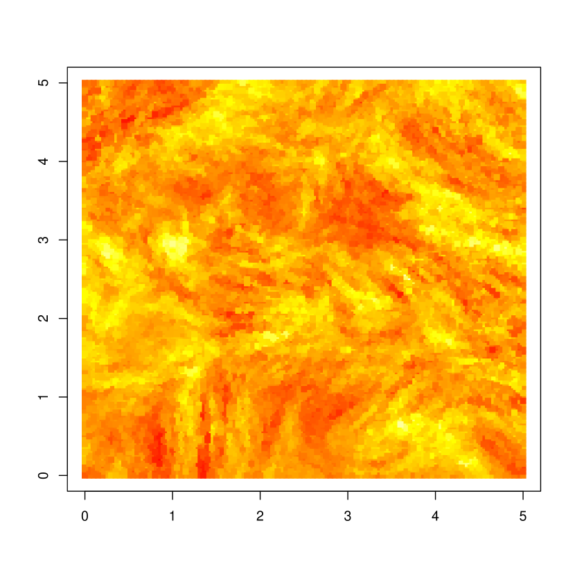
(c) NNGP samples corresponding to the ellipses

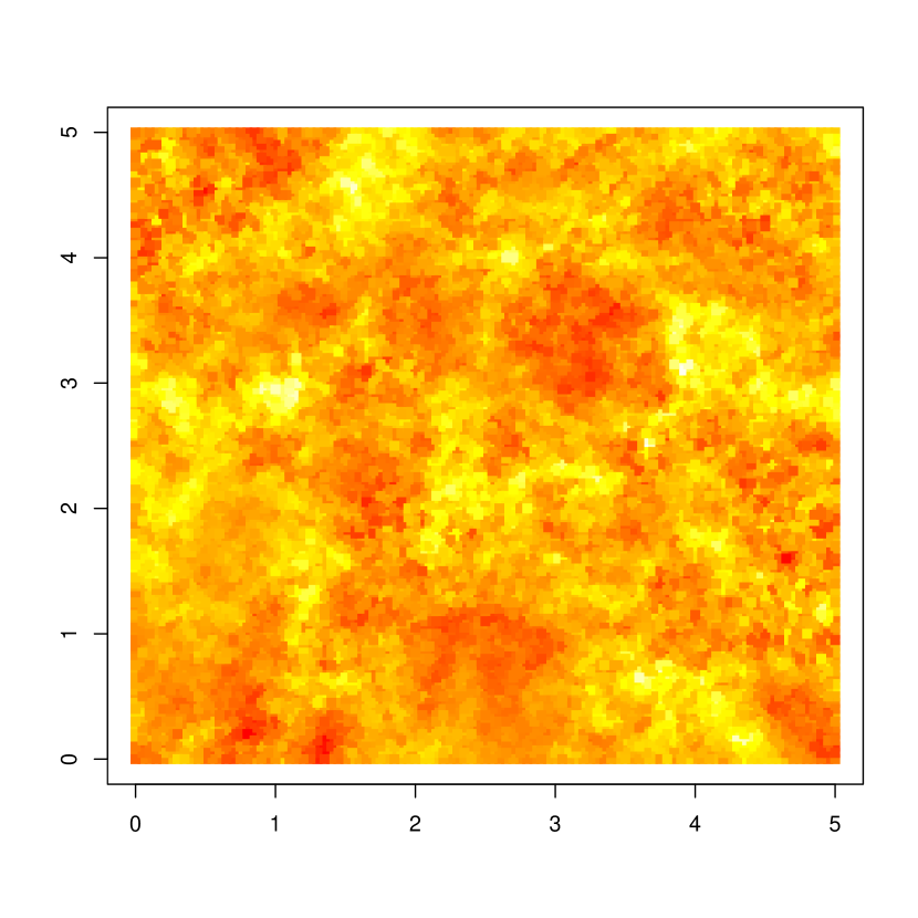
(d) NNGP samples corresponding to the circles

Figure 1: Example of range ellipses and GP samples induced by the log-NNGP and matrix log-NNGP priors

4 MCMC algorithms

4.1 Ancillary-Sufficient Interweaving Strategy

The problem of high correlation between latent fields and higher-level parameters is well-known in stationary spatial models, and several solutions exist such as blocking (Knorr-Held and Rue,, 2002), collapsing (Finley et al.,, 2019) or interweaving (Filippone et al.,, 2013). Interweaving takes advantage of the discordance between two parametrizations of a latent field to sample high-level parameters. When those two parametrizations are an ancillary-sufficient couple, we have an Ancillary-Sufficient Interweaving Strategy (AS-IS); (see Yu and Meng,, 2011) and also Section C.1.

In our application, we interweave the whitened and natural parametrizations of the latent field $w(\mathcal{S})$ from (11) (a) in order to update the higher-level parameters $W_{\theta}(\mathcal{S})$ and $\beta_{\theta}$ impacting the covariance structure decomposed in (11) (c) and (12). The so-called natural parametrization of the latent field is found in the decomposition (11) (a), and is a sufficient parametrization. The whitened parametrization of the latent field is ancillary, and is obtained by multiplying the natural parametrization with the right NNGP factor of its prior precision matrix from (11) (b): $w^{*}(\mathcal{S})=(\tilde{\Sigma}({\cal S};\theta({\cal S})))^{-1/2}w(\mathcal{S}).$ The consequence of whitening is that the prior distribution (11) (b) becomes a standard normal distribution, hence the method’s name. The covariance parameters have no effect anymore on the prior distribution of the latent field. In turn, they acquire a role in the decomposition of the data. In (11)(a), $w(s_{i})$ replaced by the $i^{th}$ element of $(\tilde{\Sigma}({\cal S};\theta({\cal S})))^{1/2}w^{*}(\mathcal{S})$, while 11(b) is replaced by $w^{*}(\mathcal{S})\sim\mathcal{N}(0,I_{|\mathcal{S}|})$. Further developments concerning the behavior of $w^{*}$ can be found in Coube-Sisqueille, (2021).

The interest parameter is sampled in two steps, one for each parametrization of the latent field. Those individual steps can be full conditional draws, random walk Metropolis steps, in our case they are Hybrid Monte-Carlo (HMC) steps. That is why, later on, two potentials will be derived for the HMC steps of each parameter.

Note that $\gamma_{\theta}$ and $\gamma_{\tau}$ are themselves covariance parameters for the latent fields $W_{\theta}$ (11 (d)) and $W_{\tau}$ (11 (f)). In order to update $\gamma_{\theta}$ and $\gamma_{\tau}$, interweaving is used as well, this time treating $W_{\theta}$ and $W_{\tau}$ as latent fields, and using their respective whitened parametrizations. In the case of $\gamma_{\theta}$, nested interweaving allows to use the whitened parametrizations of $W_{\theta}(\mathcal{S})$ and $w(\mathcal{S})$. Nested interweaving also is used to update $\beta_{\theta}$ and $\beta_{\tau}$, using centering from Coube-Sisqueille and Liquet, (2021). Those technical operations are laid out in detail in Section  C.2.

4.2 Hybrid Monte-Carlo

Hybrid Monte-Carlo (HMC) (Neal et al.,, 2011) has already been implemented successfully by Heinonen et al., (2016) for nonstationary Gaussian processes. Our approach differs in two aspects. First, we use NNGP instead of full GP and, hence, derive the non-trivial differentiation of the NNGP-induced potential. Second, we use an “HMC within AS-IS” algorithm and must find the gradients of the potential for the covariance parameters using both ancillary and sufficient parametrizations.

We update the log-NNGP latent fields using HMC. Let $W_{\lambda}(\mathcal{S})$ be a field of parameters, either $\lambda=\theta$ in (11)(c) and (12), or $\lambda=\tau$ in (11)(e), and let $\zeta_{\lambda}$ be the associated log-NNGP prior covariance matrix, either $\zeta_{\theta}$ in (11)(d) or $\zeta_{\tau}$ in (11)(f). The negated log likelihood with respect to the field $W_{\lambda}(\mathcal{S})$ will then be, up to a multiplicative constant, $H_{W_{\lambda}}=-\log(f(W_{\lambda}(\mathcal{S})|\zeta_{\lambda}))-g_{\lambda}(W_{\lambda}(\mathcal{S}))$, where $f(\cdot)$ is the Normal density function involved in the log-NNGP prior and $g_{\lambda}(\cdot)$ is specified based upon the role of the parameter in the model and the chosen parametrization of the latent field in interweaving. Introducing the NNGP prior covariance of $W_{\lambda}$, we obtain $\nabla_{W_{\lambda}}H_{W_{\lambda}}=\zeta_{\lambda}^{-1}W_{\lambda}-\nabla_{W_{\lambda}}g_{\lambda}(W_{\lambda}(\mathcal{S})).$ In order to improve the efficiency of the HMC step using prior whitening (Heinonen et al.,, 2016; Neal et al.,, 2011), we consider the gradient with respect to $W_{\lambda}^{*}(\mathcal{S})=\zeta_{\lambda}^{-1/2}W_{\lambda}(\mathcal{S})$ (with $\zeta_{\lambda}^{-T/2}\zeta_{\lambda}^{-1/2}=\zeta_{\lambda}^{-1})$, with $\zeta_{\lambda}^{-T/2}=(\zeta_{\lambda}^{-1/2})^{T}$. This gradient is given as

$$\nabla_{W_{\lambda}^{*}}H_{W_{\lambda}}=\zeta_{\lambda}^{-1/2}W_{\lambda}-\zeta_{\lambda}^{T/2}\nabla_{W_{\lambda}}g_{\lambda}(W_{\lambda}(\mathcal{S})).$$ (13)

Details are provided in Section D.1. Using NNGPs to specify $\zeta_{\lambda}$ makes $\zeta_{\lambda}^{-1/2}$ sparse and triangular, which enables fast solving and multiplication. This transform is the same as the whitening presented in Section 4.1, but here we use whitening to achieve approximate decorrelation between the components, while in Section 4.1 we constructed an ancillary-sufficient couple. What remains is computing $\nabla_{W_{\lambda}}g_{\lambda}(W_{\lambda}(\mathcal{S}))$. When the marginal variance of the NNGP field is considered, that is $\lambda=\sigma$, (9) and (10) allow to derive the gradients. Details are provided in Section D.3. When the range of the NNGP field is considered, that is $\lambda=\alpha$, we find the gradient using a two-step method. The first part is to compute the derivatives of $\tilde{R}$ with respect to $W_{\alpha}$, $\tilde{R}$ being the NNGP factor such that, in equation (11)(b), we have $\tilde{\Sigma}({\cal S};\theta({\cal S}))=(\tilde{R}^{T}\tilde{R})^{-1}$. The details are presented in Section D.4. In Section  D.5, we give an estimate of the required flops and RAM. The second step, laid out in Section  D.6 is to express the gradients using the derivatives of $\tilde{R}$. We estimate the cost of this second step in Section  D.7. The last case is the variance of the noise, $\lambda=\tau$, presented in Section  D.8. In that case, only the natural parametrization of the latent field is used.

After the latent fields, we focus on the HMC update of the linear effects coefficients, either $\beta_{\theta}$ in (11) (c), $\beta_{\tau}$ in (11) (e), or $B_{j}$ in (12). This method is especially useful for the range parameters since it avoids an unaffordable Metropolis-within-Gibbs sweep over $\beta_{\alpha}$. Since we put an improper constant prior on $\beta_{\theta}$, those parameter impact the negated log-density only through their role in the decomposition of $\lambda$. Using the Jacobian chain rule, for $\lambda=\theta,\tau,$

$$\nabla_{\beta_{\lambda}}H=J_{\beta_{\lambda}}^{T}log(\lambda)\cdot\nabla_{log(\lambda)}H=X_{\lambda}^{T}\cdot\nabla_{log(\lambda)}H.$$

In the case of the log-range and log-variance, there is a one-to-one correspondence between $log(\theta)$ and $W_{\theta}$, so that it is possible to replace $\nabla_{log(\theta)}H$ by $\nabla_{W_{\theta}}g_{\theta}(W_{\theta})$. In the case of the noise variance, there can be several observations at the same spatial site. It is straightforward to derive $\nabla_{log(\tau^{2})}H$ using $\frac{\partial H}{\partial\tau^{2}_{i}(s)}=\frac{\partial l(z_{i}(s)|\tau^{2}_{i}(s),w(s),X_{i}(s),\beta)}{\partial\tau^{2}_{i}(s)}$ ($i$ being the index of the observation at site $s$).

We now focus on a last point: the covariance parameters for $W_{\theta}$ and $W_{\tau}$, respectively denoted $\gamma_{\theta}$ and $\gamma_{\tau}$ in (11). Like before, we denote $\lambda=\theta,\tau$. Here, the nested interweaving strategy is used. When the ancillary parametrization $W^{*}=\zeta^{-1/2}_{\gamma_{\lambda}}W_{\lambda}$ is used, changing $\gamma_{\lambda}$ has an impact on $W_{\lambda}$. Using the Jacobian chain rule,

$$\nabla_{\gamma_{\lambda}}H=J_{\gamma_{\lambda}}^{T}W_{\lambda}\cdot\nabla_{W_{\lambda}}H=J_{\gamma_{\lambda}}^{T}(\zeta_{\gamma_{\lambda}}^{1/2}W_{\lambda}^{*})\cdot\nabla_{W_{\lambda}}H.$$

In the case of elliptic range parameters, we have in virtue of the “Vec trick” :

$$\nabla_{S}H=J_{S}^{T}w_{A}\cdot\nabla_{w_{A}}H=J_{S}^{T}(S^{1/2}\otimes\tilde{R}_{A}^{-1}w_{A}^{*})\cdot\nabla_{w_{A}}H=J_{S}^{T}(Vec(\tilde{R}_{A_{0}}^{-1}w_{A}^{*}(S^{1/2})^{T}))\cdot\nabla_{w_{A}}H.$$

In order to get the Jacobian, the derivatives of $S^{1/2}$ with respect to $S$ are obtained by finite differences. The derivatives of $\tilde{R}_{A_{0}}^{-1}w_{A}^{*}(S^{1/2})^{T}$ are in turn obtained by matrix multiplication, and plugged into the $Vec(\cdot)$ operator.

5 APPLICATIONS OF THE MODEL

Our model is implemented and available at the public repository https://github.com/SebastienCoube/Nonstat-NNGP.

5.1 Synthetic experiments

The impact of nonstationary modeling is explored in an experiment on simulated data sets presented in Section E. Three indicators were monitored: the Deviance Information Criterion (DIC) (Spiegelhalter et al.,, 1998) (Figures 7(h), 10(c)), the mean square error (MSE) of the predicted field at unobserved sites (Figures 8(h), Section 11(c)), and the MSE of the smoothed field at observed sites (Figures 9(h), 12(c)).

In terms of DIC, it is clear that nonstationary modeling must be chosen over stationary modeling when the data is nonstationary. As for prediction at unobserved locations, a nonstationary noise variance sharply improves the MSE in relevant case (Figure 8(g)). The other parameters seem to have little effect. In terms of MSE at the observed locations, the nonstationary model brings a clear improvement in all cases.

For all three aforementioned indicators, it seems that over-modelling does not hurt. The boxplots corresponding to the “right” models are at the same level as the boxplots corresponding to over-modeling. As we shall see in the next paragraph, over-modeling does not affect the performance of the model because the non-stationary model encompasses the stationary model, and boils down to stationarity when confronted with stationary data. When stationary data is analyzed with a non-stationary model, the marginal variance parameter of the log-NNGP prior sticks to $0$, inducing a degenerate distribution. The parameter latent field ends up being constant, effectively inducing a stationary model. However, the problem of wasting time and resources fitting a complex and costlier model remains.

In those test data sets, over-modeling can be detected just by looking at the MCMC chains, without needing to wait for full convergence. For example, in Figure 2 we can see the $2000$ first states, for 3 separate chains, of the log-variance parameter for a range log-NNGP prior. On the left, the data is stationary, and the log-variance is very low. On the right, the data is non-stationary, and the log-variance is high enough to allow the parameter to move in the space. As for the model with anisotropic range parameters, it is also possible to detect over-modeling from the estimates. In order to do so, we look at the matrix logarithm of $S$ from (12). If $S\approx v^{T}\sigma^{2}v$, $v$ being the projection of $I_{d}/\sqrt{d(d+1)/2}$ in the chosen basis of symmetric matrices, then the model is effectively a nonstationary scalar range model. If $S$ is null, the model is stationary. We monitor three indicators:

$$v~{}log(S)~{}v^{T},~{}~{}~{}~{}~{}u~{}log(S)~{}u^{T},~{}~{}~{}~{}~{}x~{}log(S)~{}x^{T}$$

with $u,x$ being a completion of $v$ in the basis of the symmetric matrices. In Figure 3, we show the behavior of the indicators for three data sets: a stationary data set (Figure 3(a)), a nonstationary data set with scalar range (Figure 3(b)), and a nonstationary data set with elliptic range (Figure 3(c)). We can see that all three components are very low in Figure 3(a), implying $S\approx\textbf{0}_{~{}3\times 3}$, which makes in turn $w_{A}$ constant, eventually inducing a stationary prior for $w$. When the range is nonstationary with scalar parameters (Figure 3(b)), $vSv^{T}$ (in black) raises while the two other indicators are low. Eventually, when the data is nonstationary with elliptic range parameters (Figure 3(c)), all three indicators are high.

(a) Stationary data

(b) Data with nonstationary range

Figure 2: Log-variance of the log-NNGP prior of the range parameter (locally isotropic model)

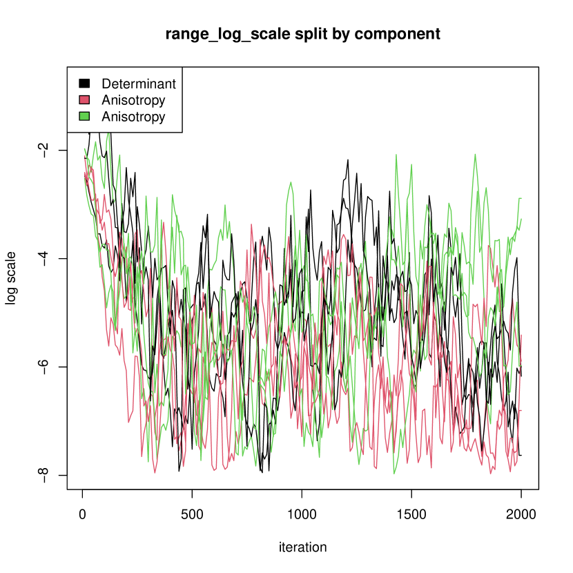
(a) Stationary data                              

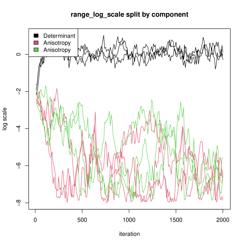
(b) Data with nonstationary scalar range

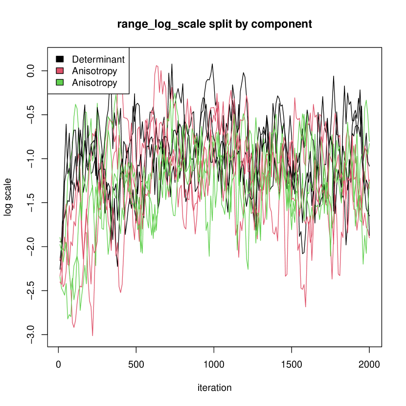
(c) Data with nonstationary elliptic range

Figure 3: Log-scale analysis of the matrix log-NNGP prior of the range parameter (locally anisotropic model)

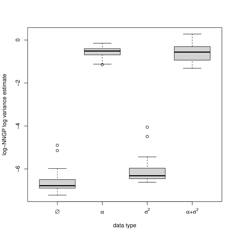
(a) Estimates of the log variance for $W_{\alpha}$

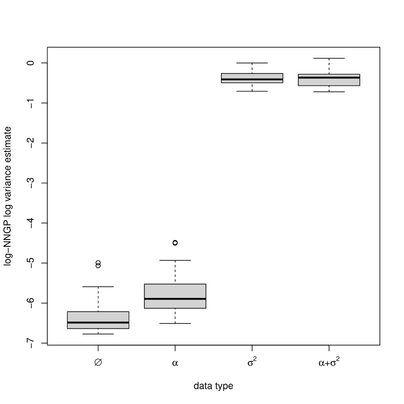
(b) Estimates of the log variance for $W_{\alpha}$

Figure 13: Estimates of the log-variance of $W_{\alpha}$ and $w_{\sigma}$ in the model $(\alpha+\sigma^{2})$ following the type of the data

A first approach to tell about the identification of parameters is to use model comparison criteria such as the DIC or MSE. If the parameters are not well-identified, then a change in the chosen model, for example replacing a model with nonstationary range by a model with nonstationary noise variance, should not affect the chosen criterion. From the experiment presented in Section  E, it is clear that nonstationary noise variance is well-identified and that forgetting it in relevant cases leads to under-fitting. The identification of nonstationary scalar range and marginal variance of the latent NNGP process is less clear, even though omitting both leads to under-fitting. On the one hand, on data with nonstationary range, a model with nonstationary variance does not do as good as a model with nonstationary range in terms of DIC and smoothing MSE (see Figures 7(d), 9(d)). On the other hand, the converse is not true for data with nonstationary variance (Figures 7(f), 9(f)); and on data with both non-stationary range and marginal variance, models with only either nonstationary range or variance do as good as the model with both (Figures 7(b) and 9(b)). This problem is not surprising: on small domains, range and variance are difficult to identify for stationary models (Zhang,, 2004). However, a troubling observation shows that there is some kind of identification: when given the possibility, our model is able to make the right choice between the two parameters. In Figure 13 in Section E, we used boxplots to summarize results of the models that estimate both nonstationary marginal variance and range. On the left (Figure 13(a)), we can see estimates for the log-variance of $W_{\alpha}$’s log-NNGP prior. On the right (Figure 13(b)), we see its counterpart for $W_{\sigma}$. In both subfigures, the boxplots are separated following the type of the data, $(\emptyset)$ being stationary data, $(\alpha)$ being data with nonstationary range, $(\sigma^{2})$ being data with nonstationary variance, and $(\alpha+\sigma^{2})$ being data with both nonstationarities (Section  E presents the naming system in detail). Recall that when the log-variance is low, the corresponding field is practically stationary. Then we can see that the right kind of nonstationarity is detected for all four configurations: when data is stationary, both log variances are very low, when the data is $(\sigma^{2})$, then only the log-variance of $W_{\sigma}$ is high, etc.

5.2 Real data analysis

5.2.1 Empirical guidelines

The full log-NNGP and matrix-log NNGP models show pathological behavior when applied to real data. It is yet to be investigated whether this is due to an intrinsic incompatibility of real data with the model architecture, or to the fact that the MCMC algorithm is not sturdy enough to run a complex model with high-dimensional data. However, the linear effects used to explain the covariance parameters behave well with real data. It is therefore possible to explain the covariance structure using environmental covariates. It is also possible to integrate spatial basis functions in the regressors in order to capture spatial patterns, see Section  F.

5.2.2 Case study: lead concentration in the United States of America mainland

The lead data set presented by Hengl, (2009) features various heavy metals measurements, including lead concentration. Various anthropic (density of air pollution, mining operations, toxic release, night lights, roads) and environmental (density of earthquakes, indices of green biomass, elevation, wetness, visible sky, wind effect) covariates are provided. Those variables may impact the emission of the lead, its diffusion, or both. The lead concentration and the covariates have been observed on $58097$ locations, with a total of $64274$ observations. As we can see in Figure 4, the measures are irregular, with large empty areas. The observations were passed to the logarithm.

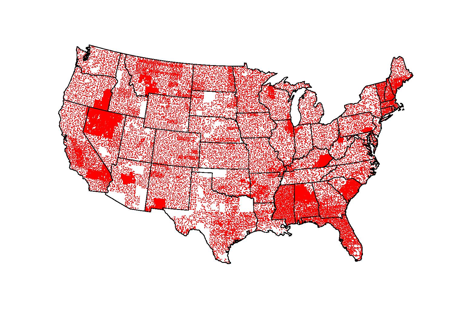
Figure 4: Measure sites for lead concentration

We used a NNGP with $10$ neighbors and the max-min order. We tested four models: a full model with non-stationary circular range, marginal variance, and noise $(\alpha+\sigma^{2}+\tau^{2})$, a model with non-stationary circular range and noise $(\alpha+\tau^{2})$, a model with just the noise $(\tau^{2})$, and a stationary model $(\emptyset)$. Each of those four models is tested with two smoothness parameters $\nu$ for the Matérn function: a rough $\nu=0.5$ (corresponding to the exponential kernel), and a smooth $\nu=1.5$. The range and the marginal variance were modeled using 25 spatial basis functions and the most spatially coherent regressors (elevation, green biomass index, and wetness index), while the noise was modeled with the basis functions and all the regressors. All runs were done with $4000$ iterations, the first $1000$ being discarded. The MCMC convergence was monitored using univariate Gelman-Rubin-Brooks diagnostics (Gelman et al.,, 1992; Brooks and Gelman,, 1998) of the high-level parameters (all the parameters of the models except the latent field $w(\mathcal{S})$). After $4000$ iterations, all the diagnostics reached a level of $1.2$ or below.

The models are compared using the DIC, the log-density of the observations, and the log-density of the predictions on validation tests where $50000$ spatial locations were kept for training (see table 1). We can see that the smoother model does worse than the rougher model in terms of DIC and log-density at the observed locations, but does better at the predicted locations, whatever the kind of nonstationarity. Therefore, we conclude that the exponential kernel is overfitting the data and we select the Matérn model with $\nu=1.5$. As for the selection of the nonstationary model, we can see that even though the full nonstationary model $(\alpha+\sigma^{2}+\tau^{2})$ does better in terms of log-density at observed locations and DIC, the model that does best in terms of predicted log density is the model with nonstationary range and noise variance $(\alpha+\tau^{2})$. We conclude that the full model over-fits the data and that a more parsimonious formulation does better. In addition to that, we remark that $(\alpha+\tau^{2})$ only brings a marginal improvement with respect to $(\tau^{2})$.

While the performances of the nonstationary model are overall much better than the stationary model’s, it is worth noticing that the former is not uniformly better that the latter. We focused on the observation-wise log-score for both smoothing and prediction, and compared the range-and-noise model with the stationary model. There was a clear spatial structure in the outcome taking value $1$ if the nonstationary model wins, and $0$ else. This spatial structure closely corresponds to the noise parameters estimated by the model, and regressing the outcome on the estimated log-range and log-noise confirms this observation: a higher noise will deteriorate the relative performances of the nonstationary model, while a higher range will not improve the smoothing but will improve the predictions. This interesting problem is to be further investigated.

Table 1: Selection criteria

model	$(\emptyset)$		$(\tau^{2})$		$(\alpha+\tau^{2})$		$(\alpha+\sigma^{2}+\tau^{2})$
smoothness	0.5	1.5	0.5	1.5	0.5	1.5	0.5	1.5
log dens unobserved	-7955	-7106	-7611	-6476	-7459	-6458	-7968	-6660
log dens observed	-30957	-35413	-26761	-31120	-25843	-29766	-24358	-28958
DIC	74508	78223	64792	68779	63460	66816	62132	66087

The predicted mean and standard deviation of the latent field are presented in Figure 5, with a comparison between stationary and nonstationary modeling. The mean nonstationary parameters are presented in Figure 6, with a decomposition between the part explained by environmental covariates and the part explained by spatial effects. The predicted means of lead contamination are quite similar between the stationary and nonstationary model. However, in regions where the range is higher, such as the Northeast, the nonstationary predictions tend to be smoother. In regions where the range is smaller, like Arizona, the nonstationary predictions are sharper, fuzzier. The predicted standard deviations are very different following whether the model is stationary or nonstationary (Figure 5(b)). In the stationary model, the only thing that imports is the spatial density of the observations (Figure 4). In the nonstationary model, regions with high spatial coherence such as the Northwest or the Western Midwest will have lower standard deviation, and other regions such as the West will have high standard deviation even if the measurements are dense there.

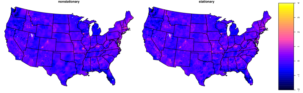
(a) Predicted latent mean of the lead concentration

(b) Predicted latent standard deviation of the lead concentration

Figure 5: Predicted mean and standard deviations of the latent field for the stationary and nonstationary models.

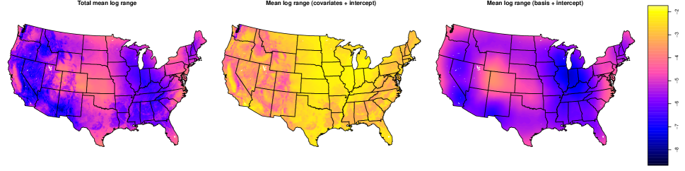
(a) Predicted range

(b) Predicted noise

Figure 6: Predicted mean of the covariance parameters in the selected nonstationary model.

6 Summary and open problems

This paper undertook to generalize the NNGP hierarchical model to nonstationary covariance structures. We delivered a proposal that takes into account the problematic aspects of computational cost, model selection, and interpretation of the parameters. Along the way, we developed various tools that could be useful in other contexts. We found a flexible and interpretable parametrization for local anisotropy, embedding the nonstationary models in a coherent family à la Russian doll. Thanks to the logarithmic transform, the user can easily interpret the parameters. This family of models seems quite resilient with respect to over-modeling, and could be useful in models that do not use NNGPs, and might combine well with additional regularizing priors. Another contribution is to bring a closed form of the derivatives of the NNGP density with respect to spatially-indexed covariance parameters. Those derivatives can be used elsewhere than in HMC, in MAP or maximum likelihood approaches for example. Eventually, in spite of problems with real-life examples, we made a step forward into showing that nested AS-IS can be a viable strategy for multi-layered hierarchical models with large data augmentations.

Regardless of our success to link environmental covariates and spatial basis functions to the covariance structure, a problem that needs further investigation is the behavior of the matrix-log NNGP model on real data. The pathological behavior of the model may be due to an intrinsic incompatibility with the data, or because of a lack of robustness of the MCMC implementation. It is worth noticing that if the spatial basis functions are obtained from a GP covariance matrix, for example Predictive Process basis functions (Banerjee et al.,, 2008; Coube-Sisqueille,, 2021) or Karhunen-Loève basis functions (Gelfand et al.,, 2010), then one only needs to put a Normal prior on the regression coefficients to obtain a low-rank GP prior. A low-rank log-GP or matrix log-GP, with fewer parameters and over-smoothing of the random effects, might be a good start to tackle the computational problems encountered by the model.

A possible extension is an implementation of the model in more than two dimensions. In particular, elliptic covariances in 3 dimensions might prove useful to quantify drifts, for example rain moving across a territory. The matter to keep in mind is that ellipses in higher dimensions incur more differentiation, since the matrix logarithm of the range parameters will have $6$ coordinates instead of $3$. A computational scale up, discussed below, may be necessary.

This, and the perspective to have coordinate spaces of dimension $3$ or more, lead us to the third point. Given the fact that we have found the gradients of the model density, the option of Maximum A Posteriori (MAP) estimation should be considered seriously. One good starting point is that the high-level parameters seem to have unimodal distributions. The MAP could be reached by tinkering the Gibbs sampler we presented into a Coordinate Descent algorithm. While an Empirical Bayes approach would do for applications such as prediction of the response variable or smoothing, finding credible intervals around the MAP would be an interesting challenge. The computational effort in flops and RAM that is not spent on MCMC could be re-invested in doing NNGP with a richer Vecchia’s approximation.

Appendix A DEMONSTRATIONS

A.1 Recursive conditional form of nonstationary NNGP

We begin with the conditional density on the left hand side of (8) and proceed as below:

$$\tilde{f}(w(s_{i})\,|\,w({\cal S}_{i-1}),\theta(\mathcal{S}))=f(w(s_{i})\,|\,w(pa(s_{i})),\theta(\mathcal{S}))\\ =f(w(s_{i}\cup pa(s_{i}))\,|\,\theta(\mathcal{S}))/f(w(pa(s_{i}))\,|\,\theta(\mathcal{S})).$$ (14)

The joint distributions $f(w(s_{i}\cup pa(s_{i}))\,|\,\theta(\mathcal{S}))$ and $f(w(pa(s_{i}))\,|\,\theta(\mathcal{S}))$ are fully specified by $\Sigma(s_{i}\cup pa(s_{i}),\theta(\mathcal{S}))$ and $\Sigma(pa(s_{i}),\theta(\mathcal{S}))$. Since the covariance functions given by (5) or (6) specify $\Sigma(s_{i},s_{j})$ using only $\{\theta(s_{i}),\theta(s_{j})\}$ instead of $\theta(\mathcal{S})$, we obtain $f(w(s_{i}\cup pa(s_{i}))\,|\,\theta(\mathcal{S}))=f(w(s_{i}\cup pa(s_{i}))\,|\,\theta(s_{i}\cup pa(s_{i})))$ and $f(w(pa(s_{i}))\,|\,\theta(\mathcal{S}))=f(w(pa(s_{i}))\,|\,\theta(pa(s_{i})))$, which is equal to $f(w(pa(s_{i}))\,|\,\theta(s_{i}\cup pa(s_{i})))$ since $w(pa(s_{i}))$ is conditionally independent of $\theta(s_{i})$ given $\theta(pa(s_{i}))$. Substituting these expressions into the right hand side of (14) yields (8).

A.2 Marginal variance of nonstationary NNGP

Let $\Sigma({\cal S})=(K(s_{i},s_{j}))$ and let $\Sigma_{0}({\cal S})=(K_{0}(s_{i},s_{j}))$ be the spatial covariance and correlation matrices, respectively, constructed from the nonstationary covariance function $K(s_{i},s_{j})$ and the corresponding correlation function $K_{0}(s_{i},s_{j})$. Let $\tilde{\Sigma}({\cal S})^{-1}=\tilde{R}^{\top}\tilde{R}$ be the NNGP precision matrix using the nonstationary covariance $K(\cdot)$, where $\tilde{R}$ is the NNGP factor of $\tilde{\Sigma}({\cal S})^{-1}$. Analogously, let $\tilde{R}_{0}$ be the NNGP precision matrix using the nonstationary correlation $\Sigma_{0}$ from (4) and either (5) or (6). If $\bar{\sigma}_{i}=\sqrt{\mbox{var}(w(s_{i})\,|\,w(pa(s_{i})))}$, then a standard expression is $\bar{\sigma}_{i}=\left(\Sigma(s_{i},s_{i})-\Sigma(s_{i},pa(s_{i}))\Sigma(pa(s_{i}),pa(s_{i}))^{-1}\Sigma(pa(s_{i}),s_{i})\right)^{1/2}$. Therefore, the $i$-th row of $\tilde{R}$ comprises (i) $1/\bar{\sigma}_{i}$ at index $i$; (ii) $-\Sigma(s_{i},pa(s_{i}))\Sigma(pa(s_{i}),pa(s_{i}))^{-1}/\bar{\sigma}_{i}$ at indices corresponding to $pa(s_{i})$; and (iii) $0$ elsewhere. Letting $\bar{\sigma}_{0i}$ be the conditional correlation obtained from $\Sigma_{0}$ instead of $\Sigma$, it is easily seen that $\bar{\sigma}_{i}=\sigma(s_{i})(\bar{\sigma}_{0i})$ using the elementary observations that $\sigma(s_{i})^{2}=\Sigma(s_{i},s_{i})$ (by definition of $\sigma(s_{i})$) and that $\Sigma({\cal A},{\cal B})=\textrm{diag}(\sigma({\cal A}))\Sigma_{0}({\cal A},{\cal B})\textrm{diag}(\sigma({\cal B}))$, where ${\cal A}$ and ${\cal B}$ are any two non-empty subsets of ${\cal S}$. Thus,

$$\begin{split}\bar{\sigma}_{i}&=\left(\Sigma(s_{i},s_{i})-\Sigma(s_{i},pa(s_{i}))\Sigma(pa(s_{i}),pa(s_{i}))^{-1}\Sigma(pa(s_{i}),s_{i})\right)^{1/2}\\ &=\sigma(s_{i})\left(\Sigma_{0}(s_{i},s_{i})-\Sigma_{0}(s_{i},pa(s_{i})\right)\Sigma_{0}(pa(s_{i}),pa(s_{i}))^{-1}\Sigma_{0}(pa(s_{i}),s_{i}))^{1/2}\\ &=\sigma(s_{i})(\bar{\sigma}_{0})_{i}\end{split}$$ (15)

Using this relationship, we can express the coefficients of row $i$ in $\tilde{R}$ as (i) $1/(\bar{\sigma}_{0i})\sigma(s_{i}))$ at position $i$; (ii) $\left(-\Sigma_{0}(s_{i},pa(s_{i}))\Sigma_{0}(pa(s_{i}),pa(s_{i}))^{-1}/\bar{(\sigma_{0})}_{i}\right)=\tilde{R}_{0}(i,pa(i))\textrm{diag}(\sigma(pa(s_{i})))^{-1}$ at the indices corresponding to $pa(s_{i})$, which means that $\tilde{R}(i,j)=\tilde{R}_{0}(i,j)/\sigma(s_{j})$ for all $s_{j}\in pa(s_{i})$; and (iii) $0$ elsewhere. Comparing elements we obtain $\tilde{R}=\tilde{R}_{0}\textrm{diag}(\sigma({\cal S}))^{-1}$.

Appendix B KL divergence between nonstationary NNGP and full nonstationary GP

B.1 Spatially indexed variances

The Kullback-Leibler (KL) divergence between two multivariate normal distributions $\mathcal{N}(\mu_{1},\Sigma_{1})$ and $\mathcal{N}(\mu_{2},\Sigma_{2})$ is

$$KL\left(\mathcal{N}_{1}\parallel\mathcal{N}_{2}\right)=\frac{1}{2}\left(\operatorname{tr}\left(\Sigma_{2}^{-1}\Sigma_{1}\right)+\left(\mu_{2}-\mu_{1}\right)^{\scriptsize{\mathrm{T}}}\Sigma_{2}^{-1}\left(\mu_{2}-\mu_{1}\right)-k+\ln\left(\frac{|\Sigma_{2}|}{|\Sigma_{1}|}\right)\right).$$

Recalling that the NNGP precision is given by $\tilde{\Sigma}({\cal S})^{-1}=\textrm{diag}(\sigma(\mathcal{S}))^{-1}(\tilde{R}_{0}^{\scriptsize{\mathrm{T}}}\tilde{R}_{0})\textrm{diag}(\sigma(\mathcal{S}))^{-1}$, that the full GP’s covariance matrix is $\textrm{diag}(\sigma(\mathcal{S}))\Sigma_{0}\textrm{diag}(\sigma(\mathcal{S}))$, and that the NNGP and GP mean are equal, the KL divergence between a nonstationary full GP with zero mean and the NNGP is $\displaystyle\frac{1}{2}\operatorname{tr}\left(\Sigma_{0}\tilde{R}_{0}^{\scriptsize{\mathrm{T}}}\tilde{R}_{0}\right)+\ln\left(\frac{|\tilde{R}_{0}^{\scriptsize{\mathrm{T}}}\tilde{R}_{0}|}{|\Sigma_{0}|}\right)$, which is the KL divergence between $N(0,\Sigma_{0})$ and $N(0,\tilde{\Sigma}_{0})$. It follows that spatially indexed variances do not affect the KL divergence between nonstationary full GPs and NNGPs.

B.2 spatially indexed variances scalar ranges

Synthetic data sets with $10000$ observations were simulated on a domain with size $5\times 5$. The spatially variable log-range had mean $log(.1)$. Three factors were tested:

• the intensity of nonstationarity, by letting the log range’s variance take different values ($0.1$, $0.3$, and $0.5$).

• the ordering (coordinate, max-min, random, middleout).

• the number of parents ($5$, $10$, $20$).

Using a linear model with interactions shows that the first factor has almost no role. The most important factor is the number of parents. Eventually, the NNGP approximation can be improved using the max-min and random order, joining Guinness, (2018)’s conclusions for stationary models in $2$ dimensions. See table 2 for more details about the effects of the factors.

B.3 Elliptic range case

Synthetic data sets with $10000$ observations were simulated on a domain with size $5\times 5$. The spatially variable log-matrix range had mean $log(.1)\times I_{2}/\sqrt{2}$. Three factors were tested:

• the intensity of nonstationarity, by letting the variance of the coordinates of the log-range matrix take different values: ($0.1\times I_{3}$, $0.3\times I_{3}$, and $0.5\times I_{3}$).

• the ordering (coordinate, max-min, random, middleout).

• the number of parents ($5$, $10$, $20$).

The outcome is treated with a linear model, whose summary is presented in table 3. Contrary to the first experiment, the intensity of the nonstationarity does play a role.

Table 2: Summary of linear regression of the KL divergence, in the scalar range case.

The reference case has coordinate ordering, $5$ nearest neighbors, and a log-range variance of $0.1$
Estimate Std. Error t value Pr($>|t|$) (Intercept) 186.5156 0.4517 412.96 0.0000 nonstat.intensity 0.3 1.4745 0.2957 4.99 0.0000 nonstat.intensity 0.5 3.2509 0.2957 10.99 0.0000 ordering max min -47.6966 0.5914 -80.66 0.0000 ordering middle out -4.7491 0.5914 -8.03 0.0000 ordering random -47.2462 0.5914 -79.89 0.0000 10 nearest neighbors -135.9274 0.5914 -229.86 0.0000 20 nearest neighbors -176.4046 0.5914 -298.31 0.0000 max min: 10 25.9771 0.8363 31.06 0.0000 middle out: 10 1.9064 0.8363 2.28 0.0228 random: 10 25.7530 0.8363 30.79 0.0000 max min: 20 41.4488 0.8363 49.56 0.0000 middle out: 20 3.3930 0.8363 4.06 0.0001 random: 20 40.9979 0.8363 49.02 0.0000

Table 3: Summary of linear regression of the KL divergence, in the elliptic range case.

The reference case has coordinate ordering, $5$ nearest neighbors, and a log-range variance of $0.1$
Estimate Std. Error t value Pr($>|t|$) (Intercept) 243.6011 1.8448 132.05 0.0000 nonstat.intensity 0.3 23.8570 1.2077 19.75 0.0000 nonstat.intensity 0.5 50.5490 1.2077 41.86 0.0000 ordering max min -50.5886 2.4154 -20.94 0.0000 ordering middle out -0.0311 2.4154 -0.01 0.9897 ordering random -50.6093 2.4154 -20.95 0.0000 10 nearest neighbors -176.3113 2.4154 -72.99 0.0000 20 nearest neighbors -238.4647 2.4154 -98.73 0.0000 max min: 10 19.4831 3.4159 5.70 0.0000 middle out: 10 -1.6965 3.4159 -0.50 0.6195 random: 10 19.5230 3.4159 5.72 0.0000 max min: 20 38.3413 3.4159 11.22 0.0000 middle out: 20 -1.6284 3.4159 -0.48 0.6337 random: 20 38.3553 3.4159 11.23 0.0000

Appendix C Details about interweaving

C.1 Interweaving

Interweaving is a method introduced by Yu and Meng, (2011), which improves the convergence speed of models relying on data augmentation. Usually various parametrizations of the data augmentation are available. For example, in the context of our NNGP model, the latent field

$$w~{}\stackrel{{\scriptstyle{a~{}priori}}}{{\sim}}~{}\mathcal{N}(0,\tilde{\Sigma})$$

with $\tilde{\Sigma}=(\tilde{R}^{T}\tilde{R})^{-1}$ can be re-parametrized as

$$w^{*}=\tilde{R}w~{}\stackrel{{\scriptstyle{a~{}priori}}}{{\sim}}~{}\mathcal{N}(0,I_{n}).$$

The component-wise interweaving strategy of Yu and Meng, (2011) can be applied when two data augmentations $w_{1}$ and $w_{2}$ have a joint distribution $[\theta,w_{1},w_{2}]$ (even if it is degenerate) such that its marginals $[\theta,w_{1}]$ and $[\theta,w_{2}]$ correspond to the two models with the different data augmentations. It takes advantage of the discordance between the two parametrizations to construct the following step in order to sample $\theta^{t+1}$:

$$[\theta,w_{2}|w_{1}^{t},\ldots]\rightarrow[\theta^{t+1},w_{1}^{t+0.5}|w_{2},\ldots],$$

“$\ldots$” being the other parameters of the model. Since all the draws are done from full conditional distributions, the target joint distribution is always preserved. Joint sampling of the parameter and the data augmentation is much easier to implement when decomposed as:

$$\underbrace{[\theta|w_{1}^{t},\ldots]\rightarrow[w_{2}|w_{1}^{t},\theta,\ldots]}_{[\theta,w_{2}|w_{1}^{t},\ldots]}\rightarrow\underbrace{[\theta^{t+1}|w_{2},\ldots]\rightarrow[w_{1}^{t+0.5}|w_{2},\theta^{t+1},\ldots]}_{[\theta^{t+1},w_{1}^{t+0.5}|w_{2},\ldots]}.$$

It is possible that the joint distribution is degenerate as long as it is well-defined, so that $[w_{2}|\theta,w_{1}]$ and $[w_{1}^{t+0.5}|w_{2},\theta^{t+1},\ldots]$ are often deterministic transformations (in our application they are). For this reason even though the data augmentation is changed at the end of the sampling of $\theta$, $w$ still has to be updated in a separate step in order to have an irreducible chain: that is why we indexed it by $t+0.5$.

The method builds its efficiency upon the fact that the parameter $\theta$ sampled in the first step, $[\theta,w_{2}|w_{1}^{t},\ldots]$, is not used later in the algorithm. This first step is therefore equivalent to $[w_{2}|w_{1}^{t},\ldots]$. If there is little correlation between the two parametrizations $w_{1}$ and $w_{2}$, the subsequent draw $[\theta^{t+1}|w_{2},\ldots]$ can produce a $\theta^{t+1}$ far from $\theta^{t}$ even if there is a strong correlation between $\theta$ and either or both $w_{1}$ and $w_{2}$.

The strategy being based on the discordance between two parametrizations, it is a good choice to pick an ancillary-sufficient couple, giving an Ancillary-Sufficient Interweaving Strategy (AS-IS). Following the terminology of Yu and Meng, (2011), $w$ is sufficient when a posteriori $(\theta|w,z)=(\theta|w)$, $z$ being the observed data and $\theta$ being the target high-level parameter. It is sufficient when it is a priori independent from $\theta$. AS-IS already proved its worth for GP models: Filippone et al., (2013) show empirically that updating covariance parameters in a Gaussian Process model benefits from interweaving the natural parametrization $w$ (sufficient) and the whitened parametrization $w^{*}$ (ancillary), while Coube-Sisqueille and Liquet, (2021) use centered and non-centered parametrizations to sample efficiently the coefficients associated with the fixed effects.

C.2 Nested interweaving for high-level parameters

The problem in our model is that there are latent fields on various layers of the model. Nested AS-IS is envisioned by Yu and Meng, (2011) for such models, even though the authors do not provide application to realistic models.

Consider a high-level parameter concerning the log-NNGP distributions of the covariance parameters. This high-level parameter may be the marginal variance of a log-NNGP distribution ($\gamma_{\theta}$, $\gamma_{\tau}$ from(11), or $S_{\theta}$ from (12)) or the regression coefficients ($\beta_{\theta}$, $\beta\tau$ from (11), or $B$ from (12)). This parameter is noted $\kappa$. Note $W_{1}$ and $W_{2}$ the parametrizations for the corresponding log-NNGP field of covariance parameters. Those parametrizations form a sufficient-ancillary pair, and can be a natural (sufficient) and whitened (ancillary) couple when we are working with marginal variance parameters (Filippone et al.,, 2013), or a centered (sufficient) and natural (ancillary) pair when working with the regression coefficients (Coube-Sisqueille and Liquet,, 2021). Eventually, note $w$ and $w^{*}$ the respectively natural and whitened parametrizations of the NNGP latent field from (12)(a).

A nested interweaving step aiming to update $\kappa$ can be devised as

$$\begin{array}[]{c}\\ \end{array}\underbrace{\begin{array}[]{c}[\kappa,W_{2},w^{*}|W_{1},w,\ldots]\rightarrow[\kappa,W_{1},w^{*}|W_{2},w,\ldots]\\ \swarrow\\ ~{}[\kappa,W_{2},w|W_{1},w^{*},\ldots]\rightarrow[\kappa,W_{1},w|W_{2},w^{*},\ldots]\end{array}}_{\text{interweaving $W$}}\left.\begin{array}[]{c}\\ \\ \\ \end{array}\right\}\rotatebox[origin={c}]{90.0}{\scriptsize{\tiny interweaving $w$}}\\$$ (16)

Like before, it is much easier to sample sequentially, for example the blocked draw
$[\kappa,W_{2},w^{*}|W_{1},w,\ldots]$ writes as

$$[\kappa|W_{1},w,\ldots]\rightarrow\underbrace{[W_{2}|\kappa,W_{1},w,\ldots]}_{\text{deterministic}}\rightarrow\underbrace{[w^{*}|\kappa,W_{1},W_{2},w,\ldots]}_{\text{deterministic}}.$$

Like before too, $W$ needs to be updated later, using an interweaving of parametrizations of $w$.

Centering-upon-whitening nested interweaving for the log-NNGP regression coefficients.

Coube-Sisqueille and Liquet, (2021) show that updating the regression coefficients of (2) using an interweaving of $w$ and $w_{center}=w+X\beta^{T}$ considerably improves the behavior of the chains, in particular when some covariates have spatial coherence. We apply this strategy to update $\beta_{\alpha}$, $\beta_{\tau^{2}}$ and $\beta_{\sigma}$.

In the case of the scalar range and the latent field’s marginal variance, we are using nested interweaving. The two relevant parametrizations for the NNGP latent field of (2) are the natural parametrization and the whitened latent field $w^{*}=\tilde{R}w$. So, for $\beta_{\alpha}$ and $\beta_{\sigma}$, the sampling step derived from (16) is

$$[\beta_{\theta}|W,w,\ldots]\rightarrow[\beta_{\theta}|W_{centered},w,\ldots]\rightarrow[\beta_{\theta}|W,w^{*},\ldots]\rightarrow[\beta_{\theta}|W_{centered},w^{*},\ldots].$$

For the sake of simplicity we do not write the implicit updates of the latent fields at each sampling of $\beta_{\theta}$. $W_{centered}$ being a sufficient augmentation, sampling from $[\beta_{\theta}|W_{centered},w,\ldots]$ is the same as sampling from $[\beta_{\theta}|W_{centered}]$. The procedure is described in Coube-Sisqueille and Liquet, (2021). As for the updates conditionally on $W$, they can be done with an usual Metropolis-within-Gibbs sweep over the components of $\beta_{\theta}$ or with a Hybrid Monte-Carlo step detailed in the following Section 4.2.

Whitening-whitening nested interweaving for the log-NNGP variance.

In the case of the marginal variance $\sigma_{\theta}\in\gamma_{\theta}$ (see (11)(g)) of a log-NNGP prior, two parametrizations of $W_{\theta}$ are available. The sufficient parametrization is the natural parametrization, while the ancillary parametrization is the whitened $w^{*}_{\theta}=\tilde{R}_{0_{\theta}}W_{\theta}/\sigma_{\theta}$, $\tilde{R}_{0_{\theta}}$ being the hyperprior correlation NNGP factor. Like before, for the latent field, we use $w$ and $w^{*}$. For the marginal variance $\sigma^{2}$, the circular range $\alpha$, and the elliptic range $A$, the step writes:

$$[\sigma_{\theta}|W_{\theta},w,\ldots]\rightarrow[\sigma_{\theta}|W_{\theta}^{*},w,\ldots]\rightarrow[\sigma_{\theta}|W_{\theta},w^{*},\ldots]\rightarrow[\sigma_{\theta}|W_{\theta}^{*},w^{*},\ldots].$$

Since $W_{\theta}$ is a sufficient statistic for $\sigma_{\theta}$, $[\sigma_{\theta}|W_{\theta},w,\ldots]$ or $[\sigma_{\theta}|W_{\theta},w^{*},\ldots]$ are equivalent to $[\sigma_{\theta}|W_{\theta}]$. The procedure to update a marginal variance with such a parametrization is well-known (Banerjee et al.,, 2008; Datta et al.,, 2016). When the ancillary parametrization $W_{\theta}^{*}$ is used, a Metropolis-Hastings step or a HMC step can be used.

Like before, only the sufficient parametrization of $w$ is used for the variance of the Gaussian noise. The step is:

$$[\sigma_{\tau}|W_{\tau},w,\ldots]\rightarrow[\sigma_{\tau}|W_{\tau}^{*},w,\ldots].$$

Appendix D Gradients for HMC updates of the covariance parameters

D.1 General form of the gradient with respect to a whitened parameter field.

Start from

$$H(W_{\lambda})=~{}-log(f_{\theta}(W_{\lambda}(\mathcal{S})|\zeta_{\lambda}))-g(W_{\lambda}(\mathcal{S}))~{}~{}\propto~{}~{}W_{\lambda}^{T}\zeta_{\lambda}^{-1}W_{\lambda}/2~{}-g(W_{\lambda}(\mathcal{S})),$$

$\zeta_{\lambda}$ being the covariance matrix induced by the log-NNGP prior. Find the gradient of $H(W_{\lambda})$ with respect to $W_{\lambda}$:

$$\nabla_{W_{\lambda}}H(W_{\lambda})=\zeta_{\lambda}^{-1}W_{\lambda}-\nabla_{W_{\lambda}}g(W_{\lambda}(\mathcal{S})).$$

Then, apply the Jacobian ($J$) chain rule $\nabla\psi\circ\phi(x)=(J^{T}\phi)(x)\cdot(\nabla\psi)(\phi(x))$ with $\psi=H(\cdot)$ et $\phi(W_{\lambda}^{*})=\zeta_{\lambda}^{1/2}W_{\lambda}^{*}$. With $J^{T}\left(\zeta_{\lambda}^{1/2}W_{\lambda}^{*}(\mathcal{S})\right)=\zeta_{\lambda}^{T/2}$, we obtain

$$\nabla_{W_{\lambda}^{*}}H(W_{\lambda})=\zeta_{\lambda}^{T/2}\zeta_{\lambda}^{-1}\zeta_{\lambda}^{1/2}W_{\lambda}^{*}-\zeta_{\lambda}^{T/2}\nabla_{W_{\lambda}}g(\zeta_{\lambda}^{1/2}W_{\lambda}^{*}(\mathcal{S}))=W_{\lambda}^{*}-\zeta_{\lambda}^{T/2}\nabla_{W_{\lambda}}g(W_{\lambda}(\mathcal{S})).$$

D.2 Gradient of the log-density of the observations with respect to the latent NNGP field.

A technical point to obtain the gradient of the log-density of the observations with respect to the latent field is that there can be several observations at the same spatial site. Consider a site $s\in\mathcal{S}$, and note these observations $obs(s)$. Note $obs(s)=\{i/M_{i,j}=1\}$ in (11) (a), that is the indices of the observations made at the spatial site $s$. We obtain, in virtue of the conditional independence of the observations of $z$ in (11) (a),

$$\begin{array}[]{ll}\frac{\partial l(z|w(\mathcal{S}),\beta,\tau(\mathcal{S}))}{\partial w(s)}&=\frac{\partial l(z_{obs(s)}|w(\mathcal{S}),\beta,\tau_{obs(s)})}{\partial w(s)}\\ &=\frac{\partial\Sigma_{x\in obs(s)}(z(x)-X(x)\beta^{T}-w(s))^{2}/2\tau(x)^{2}}{\partial w(s)}\\ &=\Sigma_{x\in obs(s)}(w(s)-(z(x)-X(x)\beta^{T}))/\tau(x)^{2}.\end{array}$$

D.3 Gradient with respect to $W_{\sigma}$

In the following, assume a variance parametrization $log(\sigma^{2}(s))=W_{\sigma}(s)+X_{\sigma}(s)\beta_{\sigma}^{T}$.

Sufficient augmentation.

When sufficient augmentation is used, the marginal variance intervenes in the NNGP density of the latent field. The resulting gradient is

$$-\nabla_{W_{\sigma}}g_{\sigma}^{sufficient}(W_{\sigma})=(1/2,\ldots,1/2)-\sigma^{-1}(\mathcal{S})~{}\circ~{}\left(\textrm{diag}(w)\tilde{R}_{0}^{T}\tilde{R}_{0}~{}\textrm{diag}(w)~{}~{}~{}\sigma^{-1}(\mathcal{S})\right)/2.$$ (17)

We start from

$$g_{\sigma}^{sufficient}(W_{\sigma})=f(w(\mathcal{S})|\alpha,\sigma(\mathcal{S})),$$

$\tilde{f}(\cdot)$ being the NNGP density from (11) (b). From (10) and (9), we write

$$\tilde{f}(w(\mathcal{S})|\alpha,\sigma(\mathcal{S}))=exp\left(-\sigma^{-1}(\mathcal{S})^{T}~{}\textrm{diag}(w)\tilde{R}_{0}^{T}\tilde{R}_{0}~{}\textrm{diag}(w)\sigma^{-1}(\mathcal{S})/2\right)\Pi_{i=1}^{n}(\tilde{R}_{0})_{i,i}/\sigma(s_{i}).$$

Passing to the negated log-density

$$\begin{array}[]{lll}-log\left(\tilde{f}(w(\mathcal{S})|\alpha,\sigma(\mathcal{S}))\right)&=&cst+\Sigma_{i=1}^{n}log(\sigma(s_{i}))~{}~{}+\\ &&\sigma^{-1}(\mathcal{S})^{T}~{}\textrm{diag}(w)\tilde{R}_{0}^{T}\tilde{R}_{0}~{}\textrm{diag}(w)\sigma^{-1}(\mathcal{S})/2.\\ \end{array}$$

One the one hand,

$$\nabla_{W_{\sigma}}\Sigma_{i=1}^{n}log(\sigma(s_{i}))=\nabla_{W_{\sigma}}\Sigma_{i=1}^{n}log((\sigma^{2}(s_{i}))^{1/2})=\nabla_{W_{\sigma}}\Sigma_{i=1}^{n}log(\sigma^{2}(s_{i}))/2=(1/2,\ldots,1/2)$$

On the other hand, using $\sigma^{-1}(s)=(\sigma^{2}(s))^{-1/2}=exp(-(W_{\sigma}(s)+X_{\sigma}(s)\beta_{\sigma}^{T})/2)$, we can write the Jacobian of $\sigma^{-1}$ with respect to $W_{\sigma}$:

$$J_{W_{\sigma}}\sigma^{-1}(\mathcal{S})=J_{W_{\sigma}}exp(-(W_{\sigma}(\mathcal{S})+X_{\sigma}(\mathcal{S})\beta_{\sigma}^{T})/2)=-\textrm{diag}(\sigma^{-1}(\mathcal{S})/2).$$

We also find the following gradient:

$$\nabla_{\sigma^{-1}}\sigma^{-1}(\mathcal{S})^{T}~{}\textrm{diag}(w)\tilde{R}_{0}^{T}\tilde{R}_{0}~{}\textrm{diag}(w)\sigma^{-1}(\mathcal{S})/2=\textrm{diag}(w)\tilde{R}_{0}^{T}\tilde{R}_{0}~{}\textrm{diag}(w)\sigma^{-1}(\mathcal{S}).$$

With the Jacobian chain rule, we combine the two previous formulas to find

$$-\nabla_{W_{\sigma}}\sigma^{-1}(\mathcal{S})^{T}~{}\textrm{diag}(w)\tilde{R}_{0}^{T}\tilde{R}_{0}~{}\textrm{diag}(w)\sigma^{-1}(\mathcal{S})/2=\sigma^{-1}(\mathcal{S})~{}\circ~{}\left(\textrm{diag}(w)\tilde{R}_{0}^{T}\tilde{R}_{0}~{}\textrm{diag}(w)~{}~{}~{}\sigma^{-1}(\mathcal{S})\right)/2,$$

with $\circ$ the Hadamard product. Combining the two terms, we have the result.

Ancillary augmentation.

When ancillary augmentation is used, the marginal variance has an impact on the observed field likelihood with respect to the latent field. The gradient writes

$$-\nabla_{W_{\sigma}}g_{\sigma}^{ancillary}(W_{\sigma})=-\nabla_{w}~{}l(z(\mathcal{S})|w,\beta,\tau)~{}\circ(w/2),$$ (18)

$\circ$ being the Hadamard product, and $\nabla_{W_{\sigma}}l(z(\mathcal{S})|w(\mathcal{S}),\beta,\tau)$ being discussed in Section  D.2. We start from

$$-g_{\sigma}^{ancillary}(W_{\sigma})=-l(z|w(\mathcal{S})=\tilde{R}^{-1}w^{*}(\mathcal{S}),\beta,\tau),$$

from (11) (a). The marginal variance affects the Gaussian density $l(\cdot)$ through $w(\mathcal{S})=\tilde{R}^{-1}w^{*}(\mathcal{S})$. Using two times the Jacobian chain rule,

$$\nabla_{W_{\sigma}(\mathcal{S})}l(z|w(\mathcal{S}),\beta,\tau)=J^{T}_{W_{\sigma}(\mathcal{S})}\sigma^{2}(\mathcal{S})J^{T}_{\sigma^{2}(\mathcal{S})}w(\mathcal{S})\nabla_{w(\mathcal{S})}l(z|w(\mathcal{S}),\beta,\tau).$$

From $log(\sigma^{2}(s))=W_{\sigma}(s)+X_{\sigma}(s)\beta_{\sigma}^{T}$, we have

$$J^{T}_{W_{\sigma}(\mathcal{S})}\sigma^{2}(\mathcal{S})=\textrm{diag}(\sigma^{2}(\mathcal{S})).$$

From the use of the ancillary parametrization, we have

$$J^{T}_{\sigma^{2}(\mathcal{S})}w(\mathcal{S})=J^{T}_{\sigma^{2}(\mathcal{S})}(\tilde{R}_{0}^{-1}w^{*})\circ\sigma(\mathcal{S})=\textrm{diag}((\tilde{R}_{0}^{-1}w^{*})\circ\sigma^{-1}(\mathcal{S})/2)$$

Combining the two previous expressions, we have

$$J^{T}_{W_{\sigma}(\mathcal{S})}\sigma^{2}(\mathcal{S})J^{T}_{\sigma^{2}(\mathcal{S})}w(\mathcal{S})=\textrm{diag}((\tilde{R}_{0}^{-1}w^{*})\circ\sigma(\mathcal{S})/2)=\textrm{diag}(w/2),$$

eventually leading to the result.

D.4 General derivative of $\tilde{R}$ with respect to nonstationary range parameters

The aim is to find $\partial\tilde{R}/\partial W_{\alpha}(s_{j})$ with $j\in 1,\ldots,n$. Let’s focus on the $i^{th}$ row of $\tilde{R}$, noted $\tilde{R}_{i,\cdot}$. The index of the row $i$ can be different from $j$. To find the derivative of $\tilde{R}_{i,\cdot}$ with respect to $W_{\alpha}(s_{j})$, we need to use the covariance matrix between $s_{i}$ and its parents $pa(s_{i})$. Let’s note $\Sigma^{i}$ the covariance matrix corresponding to $(pa(s_{i}),s_{i})$, and let’s block it as $\Sigma^{i}=\left[\begin{array}[]{c|c}\Sigma^{i}_{11}&\Sigma^{i}_{12}\\ \hline\cr\Sigma^{i}_{21}&\Sigma^{i}_{22}\end{array}\right]$ $\Sigma^{i}_{11}$ being a $m\times m$, with $m=|pa(s_{i})|$, covariance matrix corresponding to $pa(s_{i})$, and $\Sigma^{i}_{22}$ being a $1\times 1$ matrix corresponding to $s_{i}$. From its construction, $\tilde{R}_{i,\cdot}$ has non-null coefficients only for the column entries that correspond to $s_{i}$ and its parents $pa(s_{i})$. Therefore there is no need to compute the gradient but for those coefficients. The diagonal element $\tilde{R}_{i,i}$ has value $1/\bar{\sigma}_{i}$, $\bar{\sigma}_{i}$ being the standard deviation of $w(s_{i})$ conditionally on $w(pa(s_{i}))$. The elements that correspond to $pa(s_{i})$ have value $-\Sigma^{i}_{21}(\Sigma^{i}_{11})^{-1}/\bar{\sigma}_{i}$.
Let’s start by the diagonal coefficient $\tilde{R}_{i,i}$:
$\begin{array}[]{lllr}\partial(\tilde{R}_{ii})/\partial W_{\alpha}(s_{j})&=&\partial((\bar{\sigma}_{i}^{2})^{-1/2})/\partial W_{\alpha}(s_{j})\\ &&\text{(chain rule)}\\ &=&-(\bar{\sigma}_{i}^{-3}/2)\times\partial(\bar{\sigma}_{i}^{2})/\partial W_{\alpha}(s_{j})\\ &&\text{(using conditional variance formula)}\\ &=&-(\bar{\sigma}_{i}^{-3}/2)\times\partial(\Sigma^{i}_{22}-\Sigma^{i}_{21}(\Sigma^{i}_{11})^{-1}\Sigma^{i}_{12})/\partial W_{\alpha}(s_{j})\\ &&\text{(product rule)}\\ &=&-(\bar{\sigma}_{i}^{-3}/2)\times\partial(\Sigma^{i}_{22})/\partial W_{\alpha}(s_{j})\\ &&+(\bar{\sigma}_{i}^{-3})~{}\times\partial(\Sigma^{i}_{21})/\partial W_{\alpha}(s_{j})(\Sigma^{i}_{11})^{-1}\Sigma^{i}_{12}\\ &&+(\bar{\sigma}_{i}^{-3}/2)\times\Sigma^{i}_{21}\partial\left((\Sigma^{i}_{11})^{-1}\right)/\partial W_{\alpha}(s_{j})\Sigma^{i}_{12}\\ &&\text{(derivative of inverse)}\\ &=&-(\bar{\sigma}_{i}^{-3}/2)\times\partial(\Sigma^{i}_{22})/\partial W_{\alpha}(s_{j})&(a)\\ &&+(\bar{\sigma}_{i}^{-3})~{}\times\partial(\Sigma^{i}_{21})/\partial W_{\alpha}(s_{j})(\Sigma^{i}_{11})^{-1}\Sigma^{i}_{12}&(b)\\ &&-(\bar{\sigma}_{i}^{-3}/2)\times\Sigma^{i}_{21}(\Sigma^{i}_{11})^{-1}\left(\partial(\Sigma^{i}_{11})/\partial W_{\alpha}(s_{j})\right)(\Sigma^{i}_{11})^{-1}\Sigma^{i}_{12}&(c)\\ \\ \end{array}$
Let’s now differentiate the coefficients that correspond to $pa(s_{i})$, located on row $\tilde{R}_{i,\cdot}$ at the left of the diagonal:
$\begin{array}[]{lllr}\partial(-\Sigma^{i}_{21}(\Sigma^{i}_{11})^{-1}/\bar{\sigma}_{i})/\partial W_{\alpha}(s_{j})&=&-\partial(\Sigma^{i}_{21}(\Sigma^{i}_{11})^{-1}\times\tilde{R}_{ii})/\partial W_{\alpha}(s_{j})\\ &&\text{(product rule)}\\ &=&-\left(\partial\Sigma^{i}_{21}/\partial W_{\alpha}(s_{j})\right)(\Sigma^{i}_{11})^{-1}\times\tilde{R}_{ii}\\ &&-\Sigma^{i}_{21}\left(\partial\left((\Sigma^{i}_{11})^{-1}\right)/\partial W_{\alpha}(s_{j})\right)\times\tilde{R}_{ii}\\ &&-\Sigma^{i}_{21}(\Sigma^{i}_{11})^{-1}\partial\tilde{R}_{ii}/\partial W_{\alpha}(s_{j})\\ &&\text{(derivative of inverse)}\\ &=&-\left(\partial\Sigma^{i}_{21}/\partial W_{\alpha}(s_{j})\right)(\Sigma^{i}_{11})^{-1}\times\tilde{R}_{ii}&(d)\\ &&+\Sigma^{i}_{21}(\Sigma^{i}_{11})^{-1}\left(\partial\Sigma^{i}_{11}/\partial W_{\alpha}(s_{j})\right)(\Sigma^{i}_{11})^{-1}\times\tilde{R}_{ii}&(e)\\ &&-\Sigma^{i}_{21}(\Sigma^{i}_{11})^{-1}\times\underbrace{\partial\tilde{R}_{ii}/\partial W_{\alpha}(s_{j})}_{\text{already known}}&(f)\\ \end{array}$
From those derivatives, it appears that the elements that are needed to get the derivative of $\tilde{R}_{i,\cdot}$ are $(\Sigma^{i})^{-1}$ and $\partial\Sigma^{i}/\partial W_{\alpha}(s_{j})$ (with $s_{j}\in s_{i}\cup pa(s_{i})$). The former can anyway be re-used in order to obtain $\tilde{R}$. The latter can be approximated using finite differences:

$$\partial\Sigma^{i}/\partial W_{\alpha}(s_{j})\approx\left(\Sigma^{i}(W_{\alpha}(s_{j})+dW_{\alpha}(s_{j}))-\Sigma^{i}(W_{\alpha}(s_{j}))\right)/dW_{\alpha}(s_{j}).$$

D.5 Computational cost of the derivative of $\tilde{R}$ with respect to nonstationary range parameters

We can see that the differentiation of $\tilde{R}_{i,\cdot}$ is non-null only for $\alpha(pa(s_{i})\cup s_{i})$ because the entries of $\Sigma^{i}$ are given by $K(s,t,\alpha(s),\alpha(t))$ with $s,t\in s_{i}\cup pa(s_{i})$. Conversely, if $W_{\alpha}(s_{j})$ moves, only the rows of $\tilde{R}$ that correspond to $s_{i}$ and its children on the DAG move as well. This means that in order to compute the derivative of $\tilde{R}$ with respect to $\alpha_{j}$, the row differentiation operation must actually be done $|ch(s_{j})|+1$ times and not $n$ times. Knowing the fact that $\Sigma_{j=1}^{n}|ch(s_{j})|=\Sigma_{j=1}^{n}|pa(s_{j})|=m\times n$ ($m$ being the number of nearest neighbors used in Vecchia approximation), we can see that row differentiation must be done $(m+1)\times n$ times in order to get all the derivatives of $\tilde{R}$ with respect to $\alpha(s_{1},\ldots,s_{n})$. Given the fact that one row has $m+1$ non-null terms and that $(m+1)\times n$ rows are differentiated, the cost in RAM to store the differentiation of $\tilde{R}$ will be $O(m+1)^{2}n$. On the other hand, the flop cost of differentiation itself may seem daunting. However, the fact that spatially-variable covariance parameters affect pairwise covariances considerably simplifies the problem. In the derivatives, there are only 3 terms that depend on $\alpha(s_{j})$, they are $\partial(\Sigma^{i}_{22})/\partial W_{\alpha}(s_{j})$, $\partial(\Sigma^{i}_{12})/\partial W_{\alpha}(s_{j})$, and $\partial(\Sigma^{i}_{11})/\partial W_{\alpha}(s_{j})$. Let’s separate the cases:

1. When $i\neq j$

   1. $\partial(\Sigma^{i}_{12})/\partial W_{\alpha}(s_{j})$ has only one non-null coefficient.

   2. $\partial(\Sigma^{i}_{11})/\partial W_{\alpha}(s_{j})$ is a $m\times m$ matrix with cross structure (non-null coefficients only for the row and the column corresponding to $s_{j}$).

   3. $\partial(\Sigma^{i}_{22})/\partial W_{\alpha}(s_{j})$ is a null $1\times 1$ matrix.

2. When $i=j$

   1. $\partial(\Sigma^{i}_{12})/\partial W_{\alpha}(s_{j})$ is a dense vector of length $m$.

   2. $\partial(\Sigma^{i}_{11})/\partial W_{\alpha}(s_{j})$ is null.

   3. $\partial(\Sigma^{i}_{22})/\partial W_{\alpha}(s_{j})$ is null. because a change in $W_{\alpha}(s_{i})$ does not affect the marginal variance of $w(s_{i})$ (a change in $w_{\sigma^{2}(s_{i})}$ does).

The costliest part of the formulas is to compute $(\Sigma^{i}_{11})^{-1}$. However, this part needs only to be computed one time since it is not affected by differentiation. Even better, $(\Sigma^{i}_{11})^{-1}$ and $\Sigma^{i}_{21}(\Sigma^{i}_{11})^{-1}$ can be used to compute $\tilde{R}$ and then recycled on the fly to compute the derivatives. The computational effort needed to get them can then be removed from the cost of the derivative and remain in the cost of $\tilde{R}$.
Applying all those remarks gives table 4.

Table 4: costs to compute $\partial\tilde{R}_{i,\cdot}/\partial(W_{\alpha}(s_{j}))$

	(a)	(b)	(c)	(d)	(e)	(f)
$i=j$	$O(1)$	$O(m)$	$0$	$O(m^{2})$	$0$	$0$
$s_{i}\in ch(s_{j})$	$0$	$O(1)$	$O(m)$	$O(m)$	$O(m)$	$0$

Using table 4 and again $\Sigma_{j=1}^{n}|ch(s_{j})|=\Sigma_{j=1}^{n}|pa(s_{j})|=m\times n$, we can see that the matrix operations should have a total cost of $O(m^{2}\times n)$. The cost of the finite difference approximation to $\partial\Sigma^{i}/\partial W_{\alpha}(s_{j})$ must be added to this. The cost of computing the finite differences in one coefficient of $\Sigma^{i}$ depends on whether isotropic or anisotropic range parameters are used. In the case of isotropic range parameters, only a recomputation of the covariance function (6) with range $exp(log(\alpha(s)+dw))$ instead of $exp(log(\alpha(s)))$ will be needed. In the other case, the SVD of $log(A)$ must be computed again. What’s more, the covariance function (5) involves the Mahalanobis distance instead of the Euclidean distance. The cost will then depend on $d$, and be higher than in the case with isotropic covariance parameters.
However, due to (4), it appears that if $W_{\alpha}(s_{j})$ moves, only the row and column of $\Sigma^{i}$ that correspond to $s_{j}$ will be affected. Moreover, due to the symmetry of $\Sigma^{i}$, the row and the column will be changed exactly the same way. Therefore, computing $\partial\Sigma^{i}/\partial W_{\alpha}(s_{j})$ involves only $m+1$ finite differences since $\Sigma^{i}$ is of size $(m+1)\times(m+1)$.
The finite difference $\partial\Sigma^{i}/\partial W_{\alpha}(s_{j})$ must be computed $m+1$ time for each row of $\tilde{R}$, and there is $n$ rows. Therefore, the total cost of the finite differences should be $O(m+1)^{2}n$
Therefore, we can hope that careful implementation of the derivative of $\partial\tilde{R}/\partial(\alpha(s_{1},\ldots,s_{n}))$ will cost $O(n(m+1)^{2})$ operations, in the same order as computing $\tilde{R}$ itself (Guinness,, 2018).

D.6 Gradient of the negated log-density with respect to $W_{\alpha}$

Sufficient augmentation.

In the case of the sufficient augmentation, the range intervenes in the NNGP prior of the latent field. The gradient writes:

$$-\frac{\partial g_{\alpha}^{sufficient}(W_{\alpha})}{\partial W_{\alpha}(s_{i})}=\left(w^{T}\tilde{R}^{T}\right)\left(\partial\tilde{R}/\partial W_{\alpha}(s_{i})\right)w+\Sigma_{j/s_{j}\in\{s_{i}\cup ch(s_{i})\}}\left(\partial\tilde{R}_{j,j}/\partial W_{\alpha}(s_{i})\right)/\tilde{R}_{j,j}.$$ (19)

Start from the negated log density of the latent field with sufficient augmentation:

$$-g_{\alpha}^{sufficient}(W_{\alpha}(\mathcal{S}))=log\left(|\tilde{R}\left(\mathcal{S},\alpha(\mathcal{S})\right)|\right)+w^{T}\tilde{R}\left(\mathcal{S},\alpha(\mathcal{S})\right)^{T}\tilde{R}\left(\mathcal{S},\alpha(\mathcal{S})\right)w\times 1/2.$$

Let’s write the derivative of the log-determinant $log(|\tilde{R}|)$:
$\begin{array}[]{lll}\partial log(|\tilde{R}|)/\partial W_{\alpha}(s_{j})&=&\partial(\Sigma_{i=1}^{n}log(\tilde{R}_{i,i}))/\partial W_{\alpha}(s_{j})\text{(because $\tilde{R}$ is triangular)}\\ &=&\Sigma_{i=1}^{n}\partial log(\tilde{R}_{i,i})/\partial W_{\alpha}(s_{j})\\ &&\text{(only the rows corresponding to $s_{j}$ and its children are affected)}\\ &=&\Sigma_{i/s_{i}\in\{s_{j}\cup ch(s_{j})\}}\partial log(\tilde{R}_{i,i})/\partial W_{\alpha}(s_{j})\\ &&\text{log-function derivative}\\ &=&\Sigma_{i/s_{i}\in\{s_{j}\cup ch(s_{j})\}}\left(\partial\tilde{R}_{i,i}/\partial W_{\alpha}(s_{j})\right)/R_{i,i}\\ \end{array}$
Let’s write the derivative of $w^{T}\tilde{R}^{T}\tilde{R}w\times 1/2$:
$\begin{array}[]{lll}\partial\left(w^{T}\tilde{R}^{T}\tilde{R}w\times 1/2\right)/\partial W_{\alpha}(s_{j})&=&\partial\left((w^{T}\tilde{R}^{T})(\tilde{R}w)\times 1/2\right)\partial W_{\alpha}(s_{j})\\ &=&\partial(w^{T}\tilde{R}^{T})/\partial W_{\alpha}(s_{j})(\tilde{R}w)\times 1/2+\\ &&(w^{T}\tilde{R}^{T})\partial(\tilde{R}w)/\partial W_{\alpha}(s_{j})\times 1/2\\ &=&(w^{T}\tilde{R}^{T})\partial(\tilde{R}w)/\partial W_{\alpha}(s_{j})\\ &=&(w^{T}\tilde{R}^{T})(\partial\tilde{R}/\partial W_{\alpha}(s_{j})w)\\ \end{array}$

Ancillary Augmentation.

When ancillary augmentation is used, the covariance parameters intervene in the density of the observations knowing the latent field. This induces:

$$-\partial g_{\alpha}^{ancillary}(W_{\alpha})/\partial W_{\alpha}(s_{i})=\nabla_{w}l(z(s_{i})|w,\beta,\tau)^{T}\tilde{R}^{-1}\left(\partial\tilde{R}/\partial(W_{\alpha}(s_{i}))\right)w,$$ (20)

Start from

$$-g_{\alpha}^{ancillary}(W_{\alpha})=-l(z|w=\tilde{R}^{-1}w^{*},X,\beta,\tau).$$

Applying differentiation, we get
$\begin{array}[]{l}\partial\left(-l(z|w=\tilde{R}^{-1}w^{*},X,\beta,\tau)\right)/\partial(W_{\alpha}(s_{j}))\\ \text{(Conditional independence)}\\ =\Sigma_{i=1}^{n}\Sigma_{x\in obs(s_{i})}-\partial\left(l(z_{x}|w(s_{i})=\left(\tilde{R}^{-1}w^{*}\right)_{i},X,\beta,\tau)\right)/\partial(W_{\alpha}(s_{j}))\\ \text{(Chain rule)}\\ =\Sigma_{i=1}^{n}-\partial\left(\tilde{R}^{-1}w^{*}\right)_{i}/\partial(W_{\alpha}(s_{j}))\times\\ ~{}~{}~{}\Sigma_{x\in obs(s_{i})}\partial\left(l(z_{x}|w(s_{i})=\left(\tilde{R}^{-1}w^{*}\right)_{i},X,\beta,\tau)\right)/\partial(w(s_{i}))\\ \text{($w^{*}$ is not changed by $\theta$)}\\ =\Sigma_{i=1}^{n}-\left(\partial\tilde{R}^{-1}/\partial(W_{\alpha}(s_{j}))w^{*}\right)_{i}\times\\ ~{}~{}~{}\Sigma_{x\in obs(s_{i})}\partial\left(l(z_{x}|w(s_{i})=\left(\tilde{R}^{-1}w^{*}\right)_{i},X,\beta,\tau)\right)/\partial(w(s_{i}))\\ \text{(Differentiation of inverse)}\\ =\Sigma_{i=1}^{n}\left(\tilde{R}^{-1}\partial\tilde{R}/\partial(W_{\alpha}(s_{j}))\tilde{R}^{-1}w^{*}\right)_{i}\times\\ ~{}~{}~{}\Sigma_{x\in obs(s_{i})}\partial\left(l(z_{x}|w(s_{i})=\left(\tilde{R}^{-1}w^{*}\right)_{i},X,\beta,\tau)\right)/\partial(w(s_{i}))\\ \text{(Recognising gradient of $l(\cdot)$ in $w$)}\\ =\nabla_{w}l(z|\tilde{R}^{-1}w^{*},X,\beta,\tau)\tilde{R}^{-1}\partial\tilde{R}/\partial(W_{\alpha}(s_{j}))\tilde{R}^{-1}w^{*}.\\ \end{array}$

D.7 Computational cost of the gradient of the negated log-density with respect to $W_{\alpha}$

Both sufficient and ancillary formulations have a partial derivative with a term under the shape:

$$u^{T}\partial\tilde{R}/\partial(W_{\alpha}(s_{j}))v,$$

with $u$ an $v$ two vectors with affordable cost.
Due to its construction, $\partial\tilde{R}/\partial(W_{\alpha}(s_{j}))$ has non-null rows only at the rows that correspond to $s_{j}$ and $ch(s_{j})$, and each of those rows has itself at most $m+1$ non-null coefficients. Sparse matrix-vector multiplication $(\partial\tilde{R}/\partial(W_{\alpha}(s_{j})))v$ therefore costs $O((m+1)\times(1+|ch(s_{j})|))$ operations. Given the fact that $\Sigma_{j=1}^{n}|ch(s_{j})|=\Sigma_{j=1}^{n}|pa(s_{j})|=n\times m$, we can expect that the computational cost needed to compute $(\partial\tilde{R}/\partial(W_{\alpha}(s_{j})))v$ for $j\in 1,\ldots,n$ will be $O(n\times(m+1)^{2})$ operations, which is affordable.
Moreover, due to the fact that $\partial\tilde{R}/\partial(W_{\alpha}(s_{j}))$ has non-null rows only at the rows that correspond to $s_{j}$ and $ch(s_{j})$, we can deduce that $(\partial\tilde{R}/\partial(W_{\alpha}(s_{j})))v$ has non-null terms only on the slots that correspond to $s_{i}$ and its children. Computing $u^{T}(\partial\tilde{R}/\partial(W_{\alpha}(s_{j})))v$ will then cost $O(ch(s_{j})+1)$ operations. Using again $\Sigma_{j=1}^{n}|ch(s_{j})|=\Sigma_{j=1}^{n}|pa(s_{j})|=n\times m$, we can deduce that (if we know already $(\partial\tilde{R}/\partial(W_{\alpha}(s_{j})))v$) computing $u^{T}(\partial\tilde{R}/\partial(W_{\alpha}(s_{j})))v$ for $j\in 1,\ldots,n$ will cost $O(n(m+1))$.

D.8 Gradient of the negated log-density with respect to $W_{\tau}$

Note that we use a variance parametrization $log(\tau^{2})=W_{\tau}+X_{\tau}\beta_{\tau}^{T}$. Here, only the sufficient parametrization is used. Due to the fact that there can be more than one observation per spatial site, we give the following partial derivative, for $s\in\mathcal{S}$:

$$-\partial g_{\tau}^{sufficient}(W_{\tau})/\partial W_{\tau}(s)=\Sigma_{x\in obs(s)}1/2-\tau^{2}(x)\times(z(x)-w(s)-X(x)\beta^{T})^{2}/2.$$ (21)

We start from the log-density of the observed field knowing its mean and its variance as described in (11):

$$g_{\tau}^{sufficient}(W_{\tau})=l(z|w(\mathcal{S}),\beta,\tau).$$

Using the conditional independence of $z$ knowing the parameters of the model, we have

$$\partial l(z|w(\mathcal{S}),\beta,\tau)/\partial(W_{\tau}(s))=\partial\Sigma_{x\in obs(s)}l(z_{x}|w(s),\beta,\tau_{x})/\partial(W_{\tau}(s)).$$

Introducing the Gaussian formula for $l(\cdot)$, we get

$$\partial\Sigma_{x\in obs(s)}l(z_{x}|w(s),\beta,\tau_{x})/\partial(W_{\tau}(s))=\partial\Sigma_{x\in obs(s)}\frac{(z_{x}-X_{x}\beta-w)}{2\tau^{2}}-\frac{log(\tau^{2})}{2}/\partial(W_{\tau}(s)).$$

Differentiating with respect to $W_{\tau}$ brings the result.

Appendix E EXPERIMENTS ON SYNTHETIC DATA SETS

We would like to investigate the improvements caused by using nonstationary modeling when it is relevant, the problems caused by using nonstationary modeling when it is irrelevant, and the potential identification and overfitting problems of the model we devised. Our general approach to find answers to those questions is to run our implementation on synthetic data sets and analyze their results. Following the nonstationary process and data model we defined using (11) and (12), there is $12$ possible configurations counting the full stationary case: $2$ marginal variance models, $2$ noise variance models, $3$ range models. In order to keep the Section readable, we use the following notation for the different models:

• $(\emptyset)$ is the stationary model.

• $(\sigma^{2})$ is a model with nonstationary marginal variance.

• $(\tau^{2})$ is a model with heteroskedastic noise variance.

• $(\alpha)$ is a model with nonstationary range and isotropic range parameters.

• $(A)$ is a model with nonstationary range and elliptic range parameters.

• Complex models are noted using “$+$”. For example, a model with nonstationary marginal variance and heteroskedastic noise variance is noted $(\sigma^{2}+\tau^{2})$.

Our approach here is to use a possibly misspecified model and see what happens. Four cases are possible:

• The “right” model, in the sense it matches perfectly the process used to generate the data (however, potential identification and overfitting problems may cause it to be a bad model in practice).

• “Wrong” models, where some parameters that are stationary in the data are non-stationary in the model, and some parameters that are stationary in the model are non-stationary in the data.

• Under-modeling, where some parameters that are stationary in the model are non-stationary in the data, but all parameters that are stationary in the data are stationary in the model.

• Over-modeling, where some parameters that are stationary in the data are non-stationary in the model, but all parameters that are stationary in the model are stationary in the data.

If a nonstationary model actually helps to analyze nonstationary data, we should see if the “right” model does better than under-modeling. The problem of overfitting will be assessed by comparing over-modeling, under-modeling, and the “right” model. If there is some overfitting, over-modeling or even “right”modeling would have worse performances than simpler models. Identification problems will be monitored by looking at the “wrong” models and under-modeling. If some model formulations are interchangeable, then some of the “wrong” models should perform as good as the “right” model. Also, if two parametrizations are equivalent, then using either parametrization should do as good as using both, therefore under-modeling should do as good as the “true” model. The models are compared using the Deviance Information Criterion (DIC) (Spiegelhalter et al.,, 1998), the smoothing MSE, and the prediction MSE.

Remember that the observations of the model at the observed sites $\mathcal{S}$ are disrupted by the white noise $\epsilon$. The true latent field, used to generate the data, is named $w_{true}$. The estimated latent field is named $\hat{w}$. The smoothing MSE is

$$MSE_{smooth}=\frac{1}{\#\mathcal{S}}~{}\Sigma_{s\in\mathcal{S}}(\hat{w}(s)-w_{true}(s))^{2}.$$

The field is also predicted at unobserved sites $\mathcal{P}$, giving the prediction MSE

$$MSE_{pred}=\frac{1}{\#\mathcal{P}}~{}\Sigma_{s\in\mathcal{P}}(\hat{w}(s)-w_{true}(s))^{2}.$$

The following method was used to create synthetic data sets.

1. $12000$ locations are drawn uniformly on a square whose sides have length $5$.

2. The $10000$ first locations are kept for training. $20000$ observations are done at these locations. First, each location is granted an observation. Then, each of the $10000$ remaining observations is assigned to a location chosen following an uniform multinomial distribution.

3. The marginal variance of the nonstationary NNGP is defined. In the case of a stationary model, $log(\sigma^{2})=0$. In the case of a nonstationary model, $log(\sigma^{2})=W_{\sigma}$, $W_{\sigma}$ being a Matérn field with range $0.5$, marginal variance $0.5$, and smoothness $1$.

4. The marginal range of the nonstationary NNGP is defined. In the case of a stationary model, $log(\alpha)=log(0.1)$. In the case of a nonstationary model with circular range, $log(\alpha)=log(0.1)+W_{\alpha}$, $W_{\alpha}$ being a Matérn field with range $0.5$, marginal variance $0.5$, and smoothness $1$. In the case of a nonstationary model with elliptic range, the three components of $vech(log(A))$ (12) are modeled independently. $\left\{\begin{array}[]{ll}vech(log(A))_{1}&=W_{\alpha}^{1}+log(0.1),\\ vech(log(A))_{2}&=W_{\alpha}^{2},\\ vech(log(A))_{3}&=W_{\alpha}^{3}+log(0.1),\end{array}\right.$

   where $W_{\alpha}^{1,2,3}$ are Matérn fields with range $0.5$, marginal variance $0.5$, and smoothness $1$. Note that $log(A)=(log(0.1))\times I_{2}$ corresponds to the isotropic case with range equal to $0.1$.

5. The nonstationary NNGP latent field is sampled using $\alpha$ and $\sigma$, using an exponential kernel as the isotropic function in (5).

6. The response variable is sampled by adding a Gaussian decorrelated noise with variance $\tau^{2}$ to the latent field.

We started with the eight models obtained by combining $(\sigma),(\alpha)$, and $(\tau)$, giving us $(\emptyset)$, $(\sigma^{2})$, $(\tau^{2})$, $(\alpha)$, $(\sigma^{2}+\tau^{2})$, $(\tau^{2}+\alpha)$, $(\sigma^{2}+\alpha)$, and $(\sigma^{2}+\tau^{2}+\alpha)$. We tested each data-model configuration, yielding $64$ situations in total. Each case was replicated $30$ times. The respective results of DIC, prediction, and smoothing, are summarized by box-plots in Figures 7(h), 8(h), and 9(h).

Second, we focused on the case of elliptic range parameters with the three models obtained by combining $(\alpha)$ and $(A)$, giving us $(\emptyset)$, $(\alpha)$, and $(A)$. Like before, we tested the $9$ data-model configurations $30$ times each. The results are summarized by box-plots in figures 10(c), 11(c), and 12(c).

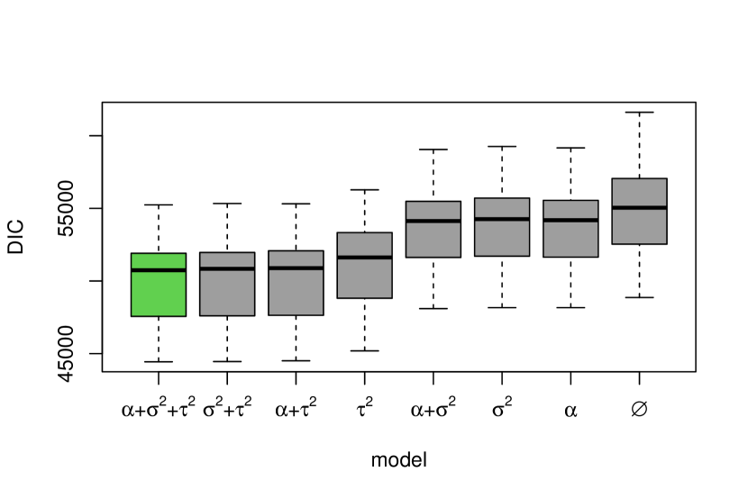
(a) $(\sigma^{2}+\tau^{2}+\alpha)$ data

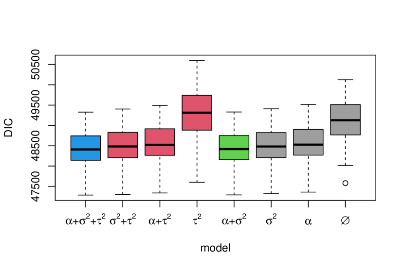
(b) $(\sigma^{2}+\alpha)$ data

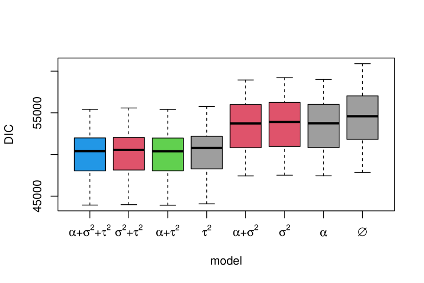
(c) $(\tau^{2}+\alpha)$ data

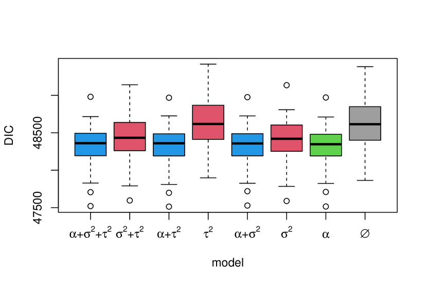
(d) $(\alpha)$ data

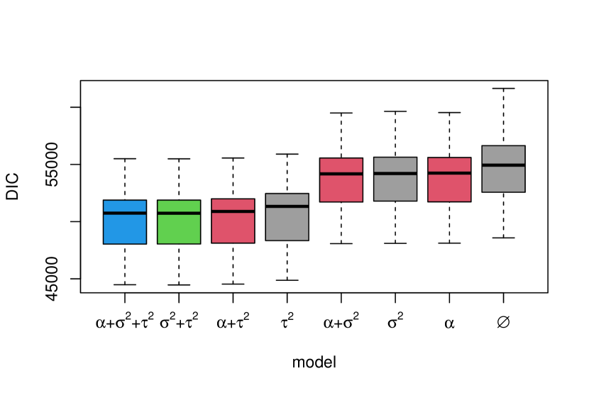
(e) $(\sigma^{2}+\tau^{2})$ data

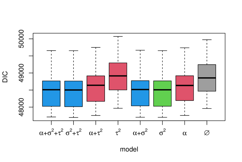
(f) $(\sigma^{2})$ data

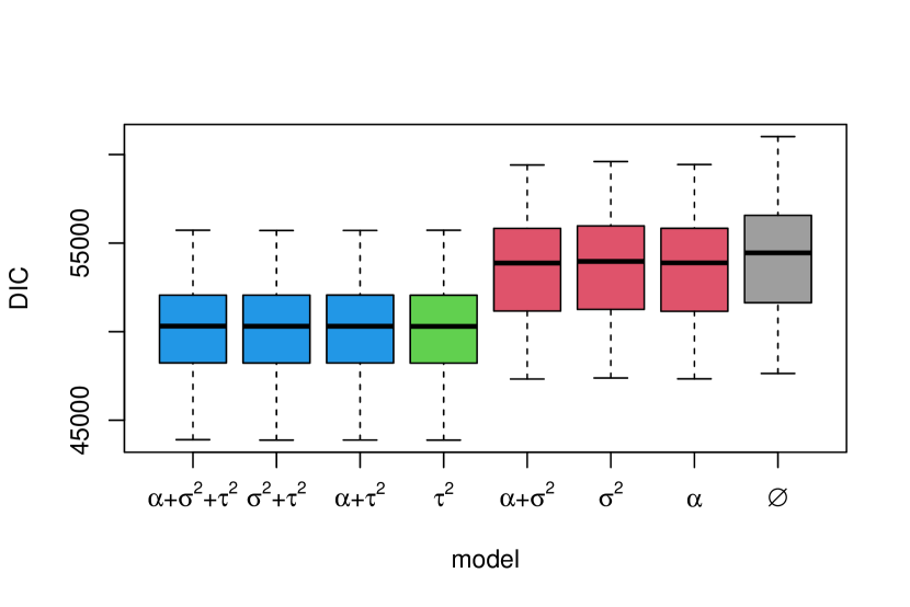
(g) $(\tau^{2})$ data

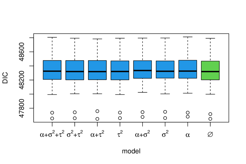
(h) $(\emptyset)$ data

Figure 7: DIC of the models for the different simulated scenarios

Legend: “right model” $\color[rgb]{0,1,0}\blacksquare\color[rgb]{0,0,0}$; “wrong model” $\color[rgb]{1,0,0}\blacksquare\color[rgb]{0,0,0}$; “over-modeling” $\color[rgb]{0,0,1}\blacksquare\color[rgb]{0,0,0}$; “under-modeling” $\color[rgb]{.5,.5,.5}\blacksquare\color[rgb]{0,0,0}$

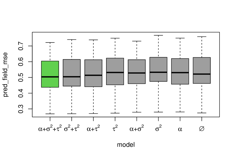
(a) $(\sigma^{2}+\tau^{2}+\alpha)$ data

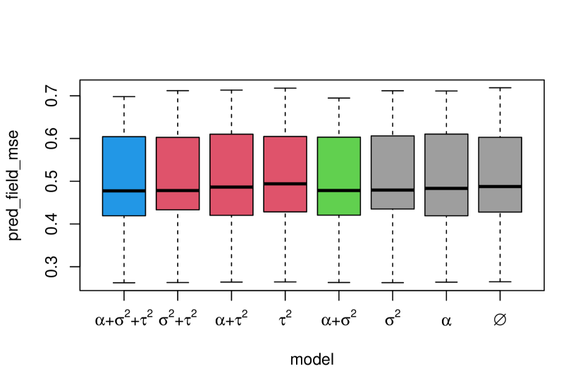
(b) $(\sigma^{2}+\alpha)$ data

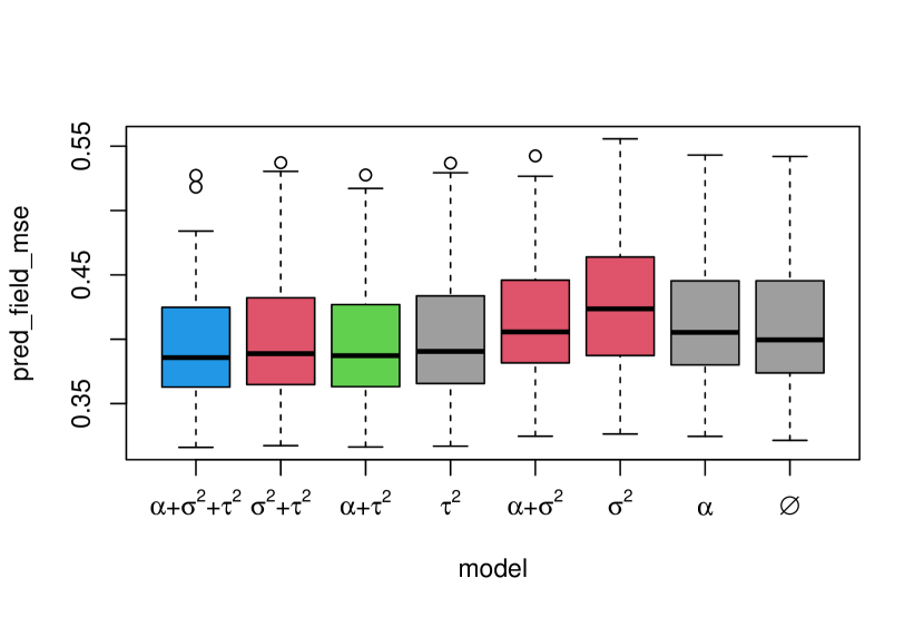
(c) $(\tau^{2}+\alpha)$ data

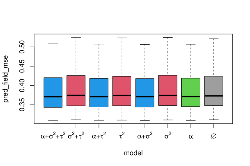
(d) $(\alpha)$ data

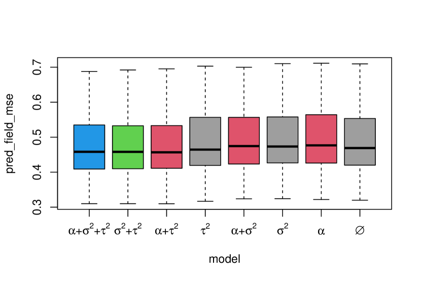
(e) $(\sigma^{2}+\tau^{2})$ data

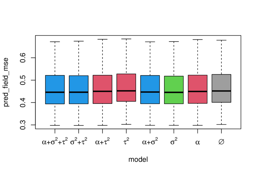
(f) $(\sigma^{2})$ data

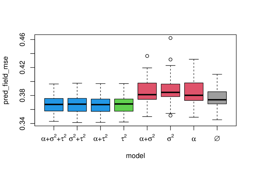
(g) $(\tau^{2})$ data

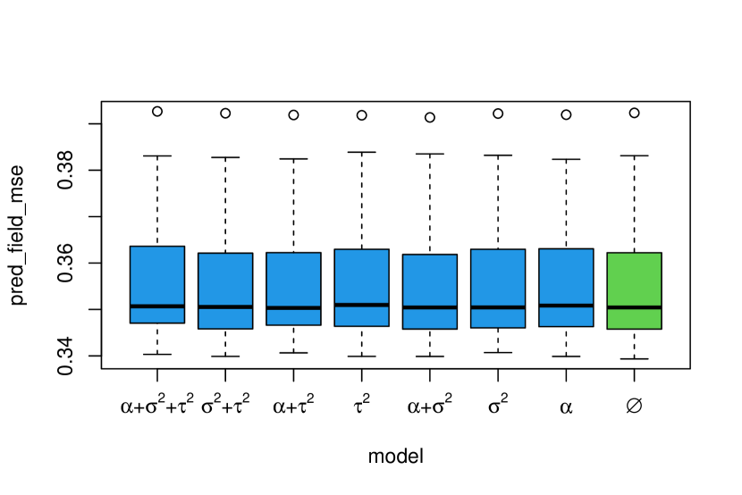
(h) $(\emptyset)$ data

Figure 8: Prediction MSE of the models for the different simulated scenarios

Legend: “right model” $\color[rgb]{0,1,0}\blacksquare\color[rgb]{0,0,0}$; “wrong model” $\color[rgb]{1,0,0}\blacksquare\color[rgb]{0,0,0}$; “over-modeling” $\color[rgb]{0,0,1}\blacksquare\color[rgb]{0,0,0}$; “under-modeling” $\color[rgb]{.5,.5,.5}\blacksquare\color[rgb]{0,0,0}$

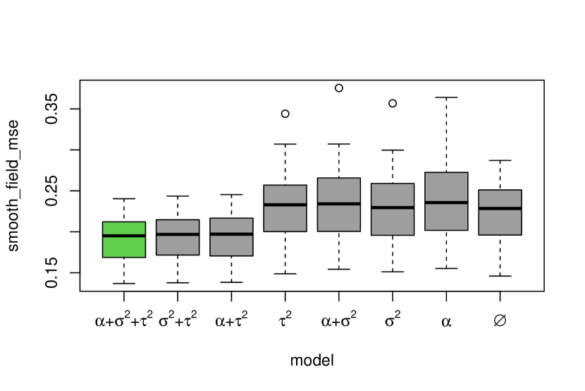
(a) $(\sigma^{2}+\tau^{2}+\alpha)$ data

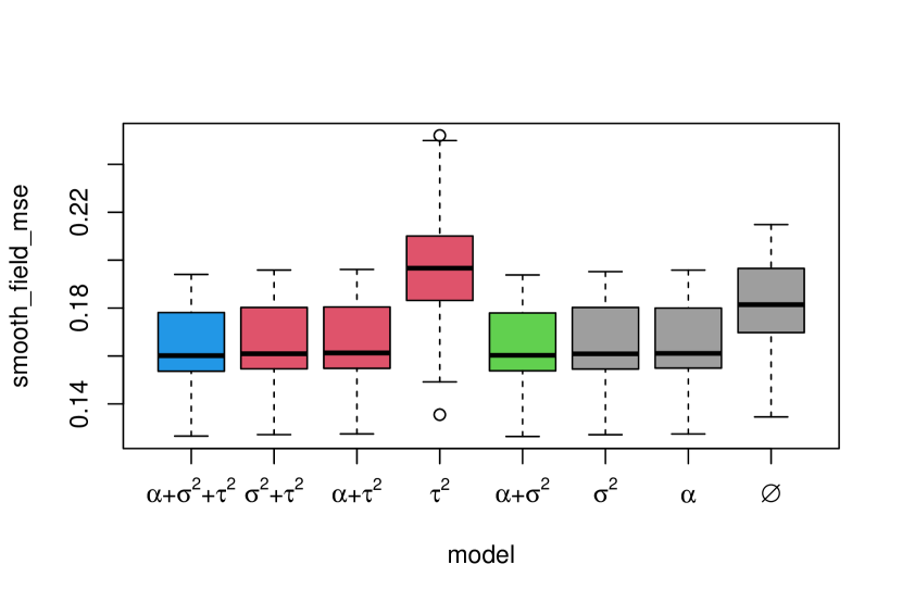
(b) $(\sigma^{2}+\alpha)$ data

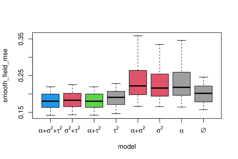
(c) $(\tau^{2}+\alpha)$ data

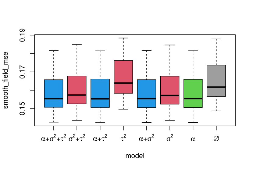
(d) $(\alpha)$ data

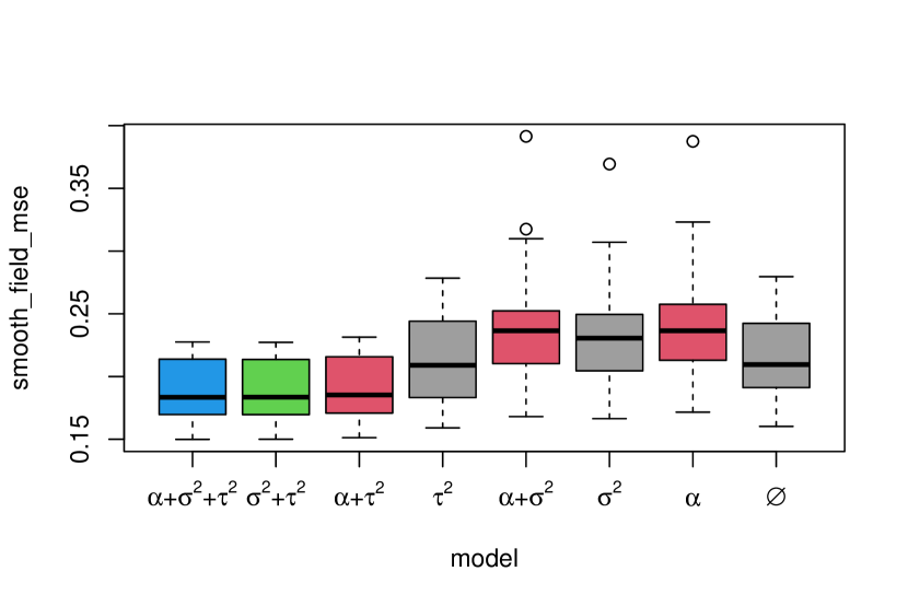
(e) $(\sigma^{2}+\tau^{2})$ data

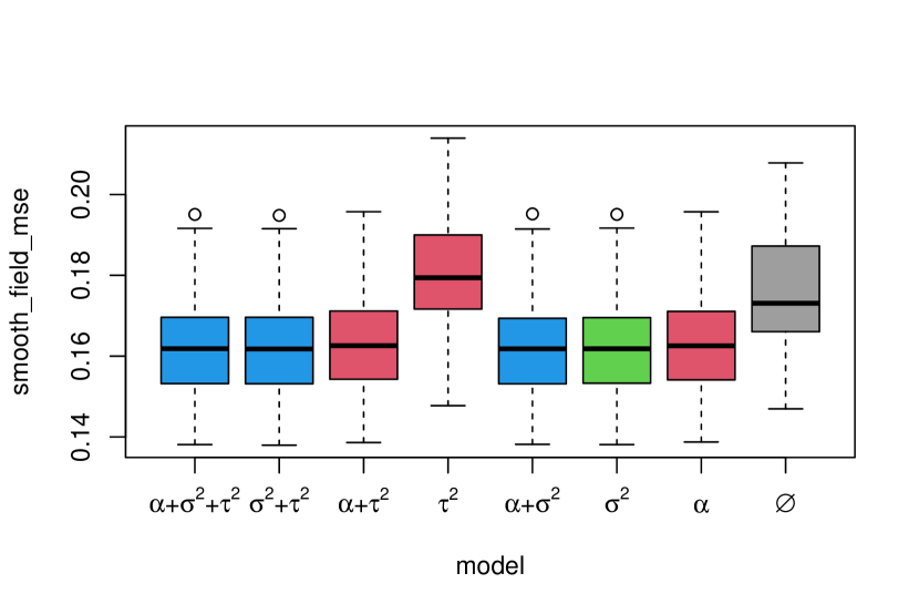
(f) $(\sigma^{2})$ data

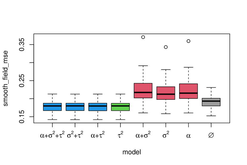
(g) $(\tau^{2})$ data

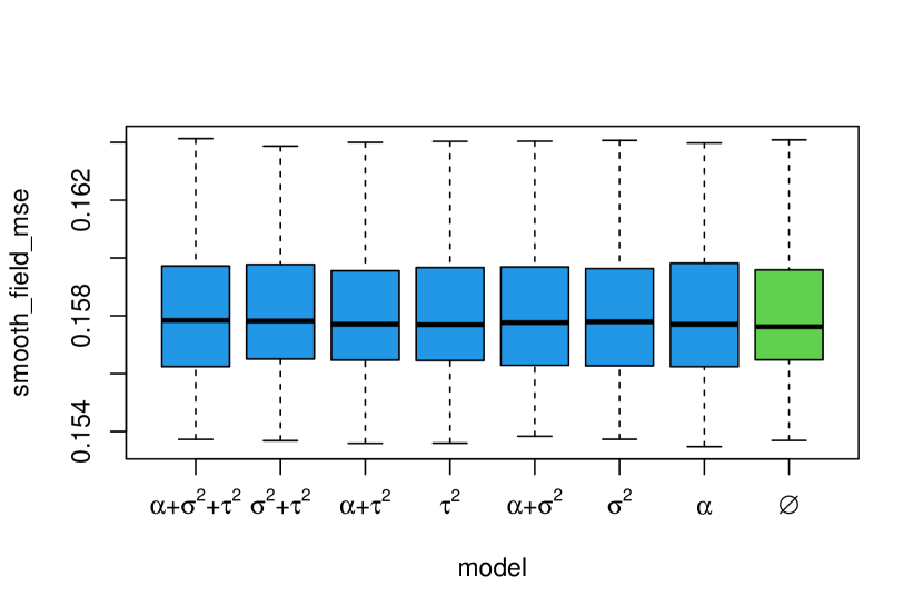
(h) $(\emptyset)$ data

Figure 9: Smoothing MSE of the models for the different simulated scenarios

Legend: “right model” $\color[rgb]{0,1,0}\blacksquare\color[rgb]{0,0,0}$; “wrong model” $\color[rgb]{1,0,0}\blacksquare\color[rgb]{0,0,0}$; “over-modeling” $\color[rgb]{0,0,1}\blacksquare\color[rgb]{0,0,0}$; “under-modeling” $\color[rgb]{.5,.5,.5}\blacksquare\color[rgb]{0,0,0}$

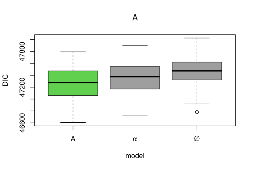
(a) $(A)$ data

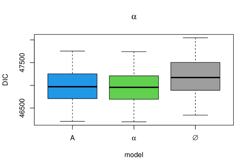
(b) $(\alpha)$ data

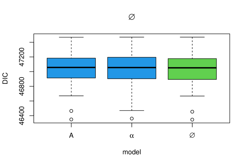
(c) $(\emptyset)$ data

Figure 10: DIC of the models for the different simulated scenarios, in the anisotropy model

Legend: “right model” $\color[rgb]{0,1,0}\blacksquare\color[rgb]{0,0,0}$; “over-modeling” $\color[rgb]{0,0,1}\blacksquare\color[rgb]{0,0,0}$; “under-modeling” $\color[rgb]{.5,.5,.5}\blacksquare\color[rgb]{0,0,0}$

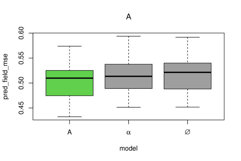
(a) $(A)$ data

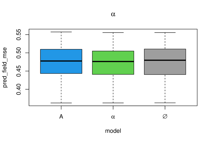
(b) $(\alpha)$ data

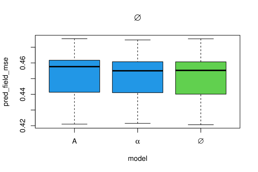
(c) $(\emptyset)$ data

Figure 11: Prediction MSE of the models for the different simulated scenarios, in the anisotropy model

Legend: “right model” $\color[rgb]{0,1,0}\blacksquare\color[rgb]{0,0,0}$; “over-modeling” $\color[rgb]{0,0,1}\blacksquare\color[rgb]{0,0,0}$; “under-modeling” $\color[rgb]{.5,.5,.5}\blacksquare\color[rgb]{0,0,0}$

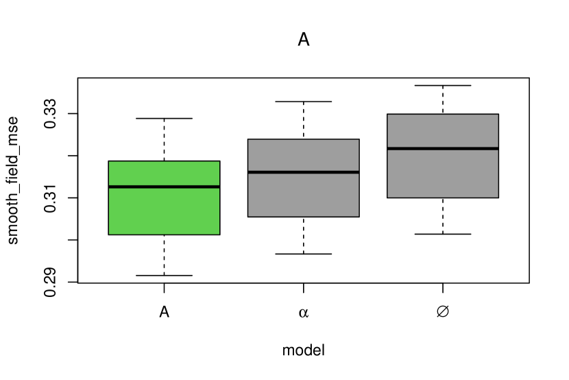
(a) $(A)$ data

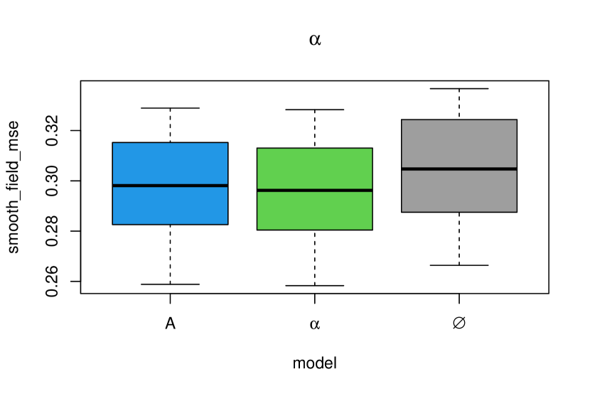
(b) $(\alpha)$ data

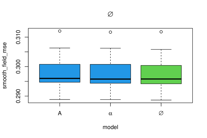
(c) $(\emptyset)$ data

Figure 12: Smoothing MSE of the models for the different simulated scenarios, in the anisotropy model

Legend: “right model” $\color[rgb]{0,1,0}\blacksquare\color[rgb]{0,0,0}$; “over-modeling” $\color[rgb]{0,0,1}\blacksquare\color[rgb]{0,0,0}$; “under-modeling” $\color[rgb]{.5,.5,.5}\blacksquare\color[rgb]{0,0,0}$

Appendix F Getting a spatial basis from a (large) NNGP factor

The basis consists in a truncated Karhunen-Loève decomposition (KLD) of a Predictive Process (PP, Banerjee et al.,, 2008) basis obtained from the NNGP used in the log-NNGP or matrix log-NNGP priors. While the PP approximation is prone to lead to over-smoothing (see the discussion in Datta et al.,, 2016), this is not a problem here since the hyperprior range is supposed to be high, inducing a smooth, large-scale prior. Start by generating a Predictive Process spatial basis of size $k$, given as :

$$B=\tilde{R}_{\theta}^{-1}M,$$

$\tilde{R}_{\theta}^{-1}$ being a NNGP factor (the same that would be used to define a log-NNGP or matrix log-NNGP prior) and $M$ being a matrix of size $n\times k$ such that $M_{i,j}=1$ if $i=j$ and $M_{i,j}=0$ everywhere else. Using fast solving relying on the sparsity and triangularity of $\tilde{R}$, this step is affordable. See Coube-Sisqueille, (2021) for developments concerning the link between NNGP and PP. Note that the first locations of $\mathcal{S}$ must be well spread over the space in order to get a satisfying PP basis. This can be obtained with the max-min or random ordering heuristics (Guinness,, 2018). The number of vectors $k$ should be large enough (a few hundred), so that there is a strong conditioning of the $n-k$ last locations. In virtue of the PP approximation, the NNGP covariance can be approached as

$$(\tilde{R}_{\theta}^{T}\tilde{R}_{\theta})^{-1}\approx BB^{T}.$$

In order to ease computation and avoid pathological MCMC behaviors that may occur with too many covariates, $B$ is summarized using truncated SVD (with for example the R package irlba by Lewis et al.,, 2019) by $B\approx UDV$, giving:

$$(\tilde{R}_{\theta}^{T}\tilde{R}_{\theta})^{-1}\approx BB^{T}\approx UDVV^{T}DU^{T}=UD^{2}U^{T}.$$ (22)

$UD^{2}U^{T}$ is an approximate Karhunen-Loève decomposition of $R_{\theta}^{T}$, and the empirical orthogonal functions (EOFs) of $U$ will be used as spatial covariates. Following Gelfand et al., (2010), the first EOFs parametrize great spatial variations, and the following EOFs represent smaller, local changes. The number of vectors of $U$ can be selected using the values of $D^{2}$ and/or looking at spatial plots of the EOFs.

Prediction at new locations can be done by prolonging the PP basis and retrieving the prolonged truncated KLD basis by linear recombination. Start by appending the predicted locations below the observed locations, and by computing a joint NNGP factor (note that the upper left corner of this factor is no other than $\tilde{R}_{\theta}$). Compute a PP basis at the predicted locations $B_{pred}$ by applying linear solving like before, and removing the first $n$ rows of the basis (they correspond to the observed locations). Then, using the SVD from (22), the KLD basis at the predicted locations $U_{pred}$ is obtained through

$$U_{pred}=B_{pred}V^{T}D^{-1}.$$

We see two potential improvements for this approach. The first is to get rid of the PP and to find a way to compute straightforwardly a truncated KLD of $(\tilde{R}_{\theta}^{T}\tilde{R}_{\theta})^{-1}$. The second is to use Gaussian priors to make this approach equivalent to a degenerate GP prior defined from a full-rank NNGP. This might lead to a more frugal and sturdier version of our log-NNGP prior.

References

- Banerjee et al., (2014) Banerjee, S., Carlin, B. P., and Gelfand, A. E. (2014). Hierarchical modeling and analysis for spatial data. CRC press.
- Banerjee et al., (2008) Banerjee, S., Gelfand, A. E., Finley, A. O., and Sang, H. (2008). Gaussian predictive process models for large spatial data sets. Journal of the Royal Statistical Society: Series B (Statistical Methodology), 70(4):825–848.
- Brooks and Gelman, (1998) Brooks, S. P. and Gelman, A. (1998). General methods for monitoring convergence of iterative simulations. Journal of computational and graphical statistics, 7(4):434–455.
- Coube-Sisqueille, (2021) Coube-Sisqueille, S. (2021). MCMC algorithms and hierarchical architectures for spatial modeling using Nearest Neighbor Gaussian Processes. PhD thesis, Université de Pau et des Pays de l’Adour.