On the (Non-)Robustness of Two-Layer Neural Networks in Different Learning Regimes

Abstract

Neural networks are known to be highly sensitive to adversarial examples. These may arise due to different factors, such as random initialization, or spurious correlations in the learning problem. To better understand these factors, we provide a precise study of the adversarial robustness in different scenarios, from initialization to the end of training in different regimes, as well as intermediate scenarios, where initialization still plays a role due to “lazy” training. We consider over-parameterized networks in high dimensions with quadratic targets and infinite samples. Our analysis allows us to identify new tradeoffs between approximation (as measured via test error) and robustness, whereby robustness can only get worse when test error improves, and vice versa. We also show how linearized lazy training regimes can worsen robustness, due to improperly scaled random initialization. Our theoretical results are illustrated with numerical experiments.

1 Introduction

Deep neural networks have enjoyed tremendous practical success in many applications involving high-dimensional data, such as images. Yet, such models are highly sensitive to small perturbations known as adversarial examples Szegedy et al. (2013), which are often imperceptible by humans. While various strategies such as adversarial training Madry et al. (2018) can mitigate this vulnerability empirically, lack of robustness remains highly problematic for many safety-critical applications like autonomous vehicles and health, and motivates a better understanding of the phenomena at play.

Various factors are known to contribute to adversarial examples. In linear models, features that are only weakly correlated with the label, possibly in a spurious manner, may improve prediction accuracy but induce large sensitivity to adversarial perturbations Tsipras et al. (2019); Sanyal et al. (2021). On the other hand, common neural networks may exhibit high sensitivity to adversarial perturbations at random initialization Simon-Gabriel et al. (2019); Daniely & Shacham (2020); Bubeck et al. (2021); Bartlett et al. (2021). Trained networks may thus involve multiple sources of vulnerability arising from initialization, training algorithms, as well as the data distribution at hand.

In this paper, we study the interplay between these different factors by analyzing approximation and robustness properties (i.e., stability of predictions, w.r.t perturbations in test data) of two-layer networks in different learning regimes. We consider two-layer finite-width networks in high dimensions with infinite data, in asymptotic regimes inspired by Ghorbani et al. (2019). This allows us to focus on the effects inherent to the data distribution and the inductive bias of architecture and training algorithms, while side-stepping issues due to finite samples. Following Ghorbani et al. (2019), we focus on regression settings with structured quadratic target functions, and consider commonly studied training regimes for two-layer networks, namely (i) neural networks with quadratic activations trained with stochastic gradient descent on the population risk, which exhibit a form of feature learning by finding the global optimum; (ii) random features (RF, Rahimi & Recht, 2008), (iii) neural tangent kernel (NT, Jacot et al., 2018), as well as (iv) “lazy” training Chizat et al. (2019) regimes for RF and NT, where we consider a first-order Taylor expansion of the network around initialization, including the initialization term itself (in contrast to the RF and NT regimes which focus on the first-order term). Note that, though the theoretical setting is inspired by Ghorbani et al. (2019), our work differs from Ghorbani et al. (2019) in its focus and scope. Indeed, we are concerned with robustness and its interplay with approximation, in different learning regimes, while Ghorbani et al. (2019) was only concerned with approximation. We also note that the lazy/linearized regimes we study as part of this work were not considered by Ghorbani et al. (2019), and help us highlight the impact of initialization on robustness.

Main contributions.

Our work establishes theoretical results which uncover novel tradeoffs between approximation (as measured via test error) and robustness that are inherent to all the regimes considered. These tradeoffs appear to be due to misalignment between the target function and the input distribution (or weight distribution) for random features (Section 5), or to the inductive bias of fully-trained networks (Sections 4 and B). We also show that improperly scaled random initialization can further degrade robustness in lazy/linearized models (Section 6), since they might inherit the nonrobustness inherent to random initialization. This raises the question of how large should the initialization be to in order to enhance the robustness of the trained model. Our theoretical results are empirically verified with extensive numerical experiments on simulated data.

The setting of our work is regression with two-layer neural networks, where we assume access to infinite training data. Thus, the only complexity parameters are the structure of the ground-truth function, the input dimension $d$ and the width of the neural network $m$, assumed to both ”large” but proportional to one another. Refer to Section 3 for details. The infinite-sample setting allows us to focus on the effects inherent to the data distribution and the inductive bias of architecture (choice of activation function) and different learning regimes, while side-stepping issues due to finite samples and label noise. Also note that in this infinite-data setting, label noise provably has no influence on the learned model, in all the learning regimes considered. The observation that there is a tradeoff between robustness and approximation, even in this infinite-sample setting, is one of the surprising findings of our work. This complements related works such as Bubeck et al. (2020b); Bubeck & Sellke (2021), which show that finite training samples with label noise is a possible source of nonrobustness in neural networks.

2 Related work

Various works have theoretically studied adversarial examples and robustness in supervised learning, and the relationship prediction performance.

Tsipras et al. (2019) considers a specific data distribution where good accuracy implies poor robustness. For example, Shafahi et al. (2018); Mahloujifar et al. (2018); Gilmer et al. (2018); Dohmatob (2019) show that for high-dimensional data distributions which have concentration property (e.g., multivariate Gaussians, distributions satisfying log-Sobolev inequalities, etc.), an imperfect classifier will admit adversarial examples. Dobriban et al. (2020) studies trade-offs in Gaussian mixture classification problems, highlighting the impact of class imbalance. On the other hand, Yang et al. (2020) observed empirically that natural images are well-separated, and so locally-lipschitz classifies shouldn’t suffer any kind of test error vs robustness tradeoff. However, gradient-descent is not likely to find such models. Our work studies regression problems with quadratic targets, and shows that there are indeed trade-offs between test error and robustness which are controlled by the learning algorithm / regime and model.

Simon-Gabriel et al. (2019); Daniely & Shacham (2020); Bubeck et al. (2021); Bartlett et al. (2021) study adversarial vulnerability of neural networks at initialization, but do not consider the effects of training the model, in contrast to our work.

Schmidt et al. (2018); Khim & Loh (2018); Yin et al. (2019); Bhattacharjee et al. (2021); Min et al. (2021b, a) study the sample complexity of robust learning. In contrasts, our work focuses on the case of infinite data, so that the only complexity parameters are the input dimension $d$ and the network with $m$. Bhattacharjee et al. (2021) studies robustness vs accuracy for data distributions which are well-separated (e.g., say the two classes are supported on disjoint balls). The main finding in that paper is that (i) the robustness vs accuracy tradeoff doesn’t exist for well-separated datasets. The work also posits that (ii) real-world datasets are well-separated. We think (i) is only an artifact of the well-separatedness assumption (an assumption which fails for Gaussians (as noted in the paper), say, due to infinite support). Also, (ii) is likely due to the fact that most real datasets are limited in sample size, and so, deceptively appear to be well-separated. Indeed, in the real world, there are cats which look like dogs (e.g, Siamese cats), even though such data might be under-represented in ML datasets.

Gao et al. (2019); Bubeck et al. (2020b); Bubeck & Sellke (2021) show that over-parameterization may be necessary for robust interpolation in the presence of noise. In contrast, our paper considers a structured problem with noiseless signal and infinite-data $n=\infty$, where the network width $m$ and the input dimension $d$ tend to infinity proportionately. In this under-complete asymptotic setting, our results show a precise picture of the trade-offs between approximation (test error) and robustness in different learning regimes. Our work nuances this picture by exhibiting a nontrivial interplay between robustness and test error which persists even in the case of infinite samples, where the model isn’t affected by label noise.

Dohmatob (2021); Hassani & Javanmard (2022) study the tradeoffs between interpolation, predictive performance (test error), and robustness for finite-width over-parameterized networks in kernel regimes with noisy linear target functions. In contrast, we consider structured quadratic target functions and compare different learning settings, including SGD optimization in a non-kernel regime, as well as lazy/linearized models.

3 Preliminaries

3.1 Notations

The set of integers from $1$ through $d$ will be denoted $[d]$. We will denote the identity matrix of size $d$ by $I_{d}$. The euclidean norm of a vector $x\in\mathbb{R}^{d}$ will be denoted $\|x\|$. The $k$th largest singular-value of a matrix $A$ will be denoted $\sigma_{k}(A)$, and equals the positive square-root of the $k$th largest eigenvalue $\lambda_{k}(AA^{\top})$ of the psd matrix $AA^{\top}$. If $A$ itself is psd then $\sigma_{k}(A)=\lambda_{k}(A)$ for any $k\in[d]$. The Frobenius norm of $A$ denoted $\|A\|_{F}$ is defined by $\|A\|_{F}:=\sqrt{\sum_{k=1}^{d}\sigma_{k}(A)^{2}}$. More generally, we define $\|A\|_{F,m}:=\sqrt{\sum_{k=1}^{m\land d}\sigma_{k}(A)^{2}}$, so that $\|A\|_{F,d}=\|A\|_{F}$ in particular. Note that $m\mapsto\|A\|_{F,m}$ is a nondecreasing function which is upper-bounded by $\|A\|_{F}$. The Hadamard / element-wise product of two compatible matrices $A_{1}$ and $A_{2}$ will be denoted $A_{1}\circ A_{2}$. The squared $L_{2}$-norm of a function $f:\mathbb{R}^{d}\to\mathbb{R}$ w.r.t the standard $d$-dimensional Gaussian distribution on $N(0,I_{d})$ will be denoted $\|f\|_{L^{2}(N(0,I_{d}))}^{2}$, and defined by $\|f\|_{L^{2}(N(0,I_{d}))}:=\mathbb{E}_{x\sim N(0,I_{d})}[f(x)^{2}],$ when this integral exists.

Hermite coefficients.

For any nonnegative integer $k$, let $\mathrm{He}_{k}:\mathbb{R}\to\mathbb{R}$ be the (probabilist’s) $k$th Hermite polynomial. For example, note that $\mathrm{He}_{0}(t):=0$, $\mathrm{He}_{1}(t):=t$, $\mathrm{He}_{2}(t)\equiv t^{2}-1$, $\mathrm{He}_{3}(t):=t^{3}-3t$, etc. The sequence $(\mathrm{He}_{k})_{k}$ forms an orthonormal basis for the Hilbert space $L^{2}=L^{2}(N(0,1))$ for functions $\mathbb{R}\to\mathbb{R}$ which are square-integrable w.r.t the standard normal distribution $N(0,1)$. Under suitable integrability conditions (refer to Section 5.1), the coefficients of the activation function $\sigma$ in this basis are called its Hermite coefficients, denoted $\lambda_{k}$, and are given by

$$\lambda_{k}=\lambda_{k}(\sigma):=\mathbb{E}_{G\sim N(0,1)}[\sigma(G)\mathrm{He}_{k}(G)].$$ (1)

Finally, $\|\sigma\|_{L^{2}(N(0,1))}^{2}=\mathbb{E}_{G\sim N(0,1)}[\sigma(G)^{2}]$ defines the squared $L_{2}$-norm of $\sigma$ w.r.t the standard Gaussian distribution $N(0,1)$. Note that by construction, one has $\|\sigma\|_{L^{2}(N(0,1))}^{2}=\sum_{k=0}^{\infty}\lambda_{k}^{2}(\sigma)$.

Asymptotics.

The usual notation $\mathcal{O}_{d}(1)$ (resp. $\mathcal{O}_{d,\mathbb{P}}(1)$) is used to denote a quantity which remains bounded (resp. bounded in probability) in the limit $d\to\infty$. Likewise $o_{d}(1)$ (resp. $o_{d,\mathbb{P}}(1)$) denotes a quantity which goes to zero (resp. which goes to zero in probability) in the limit $d\to\infty$. As usual, the acronym ”a.s” stands for almost-surely, while ”w.p $p$” stands for with probability at least $p$.

3.2 Ground truth / teacher model.

We consider the following regression setup proposed in Ghorbani et al  Ghorbani et al. (2019). Let $B$ be a fixed $d\times d$ psd matrix and let $b_{0}\in\mathbb{R}$ be a fixed unknown scalar. Consider the following quadratic target model

$$f_{\star}(x):=x^{\top}Bx+b_{0},\;\forall x\in\mathbb{R}^{d}.$$ (2)

We assume the input data is distributed according to $N(0,I_{d})$, the standard Gaussian distribution in $d$ dimensions. Thus, the structure of the problem of learning the ground-truth function $f_{\star}$ in (2) is completely determined by the unknown $d\times d$ matrix $B$. We assume an idealized scenario where the learner has access to an infinite number of iid samples of the form $(x,f_{\star}(x))$ with $x\sim N(0,I_{d})$. For simplicity of analysis, we will further assume as in Ghorbani et al. (2019) that the ground-truth function $f_{\star}$ defined in (2) is centered, i.e $\mathbb{E}_{x\sim N(0,I_{d})}[f_{\star}(x)]=0$. This forces the offset $b_{0}$ to be equal to $-\mathrm{tr}(B)$.

3.3 Finite-width two-layer neural network

Consider a two-layer neural network

$$f_{W,z,s}(x) :=\sum_{j=1}^{m}z_{j}\sigma(x^{\top}w_{j})-s,$$ (3)

where $m$ is the network width, i.e., the number of hidden neurons each with parameter vector $w_{j}\in\mathbb{R}^{d}$, output weights $z=(z_{1},\ldots,z_{m})\in\mathbb{R}^{m}$, and activation function $\sigma:\mathbb{R}\to\mathbb{R}$. We define $W$ as the $m\times d$ matrix with $j$th row $w_{j}$. The scalar $s$ is an offset which we will sometimes set to zero, in which case we will simply write $f_{W,z,s}:=f_{W,z,0}$.

Asymptotic regime with infinite data.

Motivated by Ghorbani et al. (2019), we will consider the following regime:

– Infinite data. The sample size $n$ is equal to $\infty$, i.e., the learner has access to the entire data distribution, allowing us to step-aside issues linked with finite samples.

– Proportionate scaling of dimensionality and width. The input-dimension $d$ and the network width $m$ are finite, and large of the same order, i.e.,

$$m,d\to\infty,\;m/d\to\rho\in(0,\infty).$$ (4)

The parameter $\rho$ (called the aspect ratio), which will play a crucial role in the sequel, corresponds to the parametrization rate: $\rho<1$ corresponds to under-parametrization, while $\rho>1$ corresponds to over-parametrization (more hidden neurons than input dimension). We will also consider the extreme over-parametrization regime corresponding to the double limit: $m,d\to\infty$, $m/d\to\rho$, $\rho\to\infty$.

The parameter $\rho$ will play a crucial role in our analysis of robustness, similar to Ghorbani et al. (2019) for approximation.

3.4 Metrics for test error and robustness

Test error.

The test / approximation error of a function $f:\mathbb{R}^{d}\to\mathbb{R}$ (e.g a neural network) is

$$\varepsilon_{{\rm test}}(f):=\|f-f_{\star}\|_{L^{2}(N(0,I_{d}))}^{2}=\mathbb{E}_{x\sim N(0,I_{d})}|f(x)-f_{\star}(x)|^{2},$$ (5)

and measures how well $f$ approximates the ground-truth function $f^{\star}$ w.r.t to the data distribution $N(0,I_{d})$. It will be instructive to compare the test error of a model with that of the null predictor, which outputs $0$ on every input $x$. To this end, we will usually consider the normalized test error,

$$\widetilde{\varepsilon}_{{\rm test}}(f):=\varepsilon_{{\rm test}}(f)/\|f_{\star}\|_{L^{2}(N(0,I_{d}))}^{2}.$$ (6)

This quantity was studied in Ghorbani et al. (2019) where explicit analytic formulae were obtained in various regimes of interest for two-layer networks: networks fully trained by stochastic gradient-descent (SGD) on the population risk, random features (RF), and neural tangent (NT). We shall consider these same regimes and establish tradeoffs between test error and robustness of the corresponding models.

Measure of robustness / stability.

We will measure the robustness of a (weakly) differentiable function $f:\mathbb{R}^{d}\to\mathbb{R}$ (e.g., the two-layer neural net (3)) by the square-root of its Dirichlet energy (aka squared Sobolev-seminorm) $\mathfrak{S}(f)^{2}$ w.r.t. to a random test point $x\sim N(0,I_{d})$, defined by setting

$$\mathfrak{S}(f)^{2}:=\|\nabla_{x}f\|_{L^{2}(N(0,I_{d}))}^{2}=\mathbb{E}_{x\sim N(0,I_{d})}\|\nabla_{x}f(x)\|^{2}.$$ (7)

The smaller the value of $\mathfrak{S}(f)$, the more robust / stable $f$ is to changes in a typical input data point, namely $x\sim N(0,I_{d})$ here. We justify the choice of this quantity as a measure of robustness in Appendix A, where we show that it may be viewed as a first-order approximation of the adversarial risk (Madry et al., 2018). Note that, stability as a measure of robustness has been considered in other works like  Bubeck et al. (2020b); Bubeck & Sellke (2021) (for regression settings) and Wu et al. (2021) (for classification settings).

It will be convenient to compare the robustness of a model $f$ to that of the baseline quadratic ground-truth function $f_{\star}$ defined in (2). To this end, the normalized measure of robustness of $f$ is

$$\widetilde{\varepsilon}_{{\rm rob}}(f):=\mathfrak{S}(f)^{2}/\mathfrak{S}(f_{\star})^{2}.$$ (8)

The objective of our paper is to study the quantity $\widetilde{\varepsilon}_{{\rm rob}}(f)$ for neural networks (3) in various regimes in the limit (4), and put to light interesting phenomena. It paints a picture complementary to Ghorbani et al. (2019).

Let us start by deriving an analytic formula for the robustness measure for the neural network general model (3). This result will be exploited in the sequel in the analysis of the different learning regimes we will consider. [] For the neural net $f_{W,z,s}$ defined in (3), we have the analytic formula $\mathfrak{S}(f_{W,z,s})^{2}=z^{\top}Cz$, where $C=C(W)$ is the $m\times m$ psd matrix with entries given by (with $x\sim N(0,I_{d})$)

$$c_{j,k}:=(w_{j}^{\top}w_{k})\mathbb{E}_{x}[\sigma^{\prime}(x^{\top}w_{j})\sigma^{\prime}(x^{\top}w_{k})]\,\forall j,k\in[m].$$ (9)

In particular, for a quadratic activation $\sigma(t)\equiv t^{2}+s$, we have $c_{j,k}=4(w_{j}^{\top}w_{k})^{2}\,\,\forall j,k\in[m].$

4 Results for fully-trained networks

Consider a neural network model $f_{\mathrm{SGD}}:\mathbb{R}^{d}\to\mathbb{R}$ given by

$$f_{\mathrm{SGD}}(x):=\sum_{j=1}^{m}(x^{\top}w_{j})^{2}+s.$$ (10)

Here, $W=(w_{1},\ldots,w_{m})\in\mathbb{R}^{m\times d}$ is a matrix of learnable parameters (one per hidden neuron), and $s\in\mathbb{R}$ is a learnable offset. The output weights vector is fixed to $z=1_{m}$, while $W$ and $c$ are optimized via SGD, where each update is on a single new sample point.

It is shown in Thm. 3 of Ghorbani et al. (2019) that if $W_{t}\in\mathbb{R}^{m\times d}$ is the matrix of hidden parameters after $t$ steps of SGD, then in the limit (4), the matrix $W_{t}W_{t}^{\top}\in\mathbb{R}^{m\times m}$ converges almost-surely to the best rank-$m$ approximation of $B$. Here, the almost-sure convergence is w.r.t randomness in the training data and in the initial random state of the parameters of the hidden neurons. Thus, by continuity of matrix norms, we deduce that $\|W_{t}W_{t}^{\top}\|^{2}_{F}$ converges a.s to $\|B\|_{F,m}^{2}$, in the infinite data limit $t\to\infty$.

Combining with Lemma 3.4 establishes the following asymptotic formula for the (normalized) robustness of the resulting model $f_{\mathrm{SGD}}$, in the high-dimensional limit (4).

[] In the limit (4), it holds that $\widetilde{\varepsilon}_{{\rm rob}}(f_{\mathrm{SGD}})\overset{a.s}{\longrightarrow}\dfrac{\|B\|_{F,m}^{2}}{\|B\|_{F}^{2}}=\dfrac{\sum_{k=1}^{m\land d}\lambda_{k}(B)^{2}}{\sum_{j=1}^{d}\lambda_{k}(B)^{2}}\leq 1,$ with equality iff $\mathrm{rank}(B)\leq m$. In particular, if $\rho\geq 1$, then in the limit (4), it holds that $\widetilde{\varepsilon}_{{\rm rob}}(f_{\mathrm{SGD}})\overset{a.s}{\longrightarrow}1$.

Tradeoff approximation and robustness.

We see from the above theorem that the robustness measure for the SGD model converges to that of the true model if $m\geq d$, namely $\mathfrak{S}(f_{\mathrm{SGD}})^{2}\to\sum_{j=1}^{d}\lambda_{j}(B)^{2}=\mathfrak{S}(f_{\star})^{2}$ if $m\geq\mathrm{rank}(B)$ (for example, if $m\geq d$). Otherwise, if $m\leq\mathrm{rank}(B)$, then the limiting value of $\mathfrak{S}(f_{\mathrm{SGD}})^{2}$ can be arbitrarily less than $\mathfrak{S}(f_{\star})^{2}$, i.e., the SGD model will be much more robust (i.e., stable) than the ground truth model. Comparing with Thm. 3 and Prop. 1 of Ghorbani et al. (2019), we can see that this increase in robustness is at the expense of increased test error. Indeed, it was shown in the aforementioned paper that the normalized test error $\widetilde{\varepsilon}_{{\rm test}}(f_{\mathrm{SGD}})$ verifies

$$\widetilde{\varepsilon}_{{\rm test}}(f_{\mathrm{SGD}})\overset{p}{\longrightarrow}1-\frac{\|B\|_{F,m}^{2}}{\|B\|_{F}^{2}},\text{ in the limit }\eqref{eq:proportionate}$$ (11)

Combining with our Thm. 4, we deduce that

$$\widetilde{\varepsilon}_{{\rm test}}(f_{\mathrm{SGD}})+\widetilde{\varepsilon}_{{\rm rob}}(f_{\mathrm{SGD}})\overset{p}{\longrightarrow}1,\text{ in the limit }\eqref{eq:proportionate}.$$ (12)

The above formula highlights a tradeoff between test error and robustness. Thus, we have identified a novel tradeoff between approximation (test error) and robustness for the neural network model (3) trained via SGD. In the sequel, we shall establish such tradeoffs for other learning regimes.

5 Results for the random features (RF) model

Consider the two-layer model (3) with hidden neuron parameters $w_{1},\ldots,w_{m}$ sampled iid from a $d$-dimensional multivariate Gaussian distribution $N(0,\Gamma)$ with covariance matrix $\Gamma$. We denote this model $f_{\mathrm{RF}}$, which is thus given by

$$f_{\mathrm{RF}}(x)=f_{W,z_{\mathrm{RF}}}(x)=z_{\mathrm{RF}}^{\top}\sigma(Wx),$$ (13)

where $z_{\mathrm{RF}}\in\mathbb{R}^{m}$ solves the following linear regression problem

$$\arg\min_{z\in\mathbb{R}^{m}}\mathbb{E}_{x\sim N(0,I_{d})}[(z^{\top}\sigma(Wx)-f_{\star}(x))^{2}].$$ (14)

The covariance matrix $\Gamma$ encompasses the inductive bias of the neurons at initialization to different directions in feature space. Define the alignment $\alpha=\alpha(B,\Gamma)$ of the hidden neurons to the task at hand, namely learning the function $f_{\star}$, as follows

$$\alpha:=\frac{\mathrm{tr}(B\Gamma)}{\|B\|_{F}\|\Gamma\|_{F}}\leq 1.$$ (15)

As we shall see, the task-alignment $\alpha$ plays a crucial role in the prediction performance (test error) and robustness dynamics of the resulting model, in the learning regimes considered in our work.

5.1 Assumptions and key quantities

As in Ghorbani et al. (2019), we will need the following technical conditions in the current section and subsection sections of this article. [] The covariance matrix $\Gamma$ of the hidden neurons satisfies the following: (A) $\mathrm{tr}(\Gamma)=1$ and $d\cdot\|\Gamma\|_{op}=\mathcal{O}(1)$. (B) The empirical eigenvalue distribution of $d\cdot\Gamma$ converges weakly to a probability distribution $\mathcal{D}$ on $\mathbb{R}_{+}$. This condition is quite reasonable, and moreover, it allows us to leverage standard tools from random matrix theory (RMT) in our analysis. We will also need the following condition.

[] The activation function $\sigma$ is weakly continuously-differentiable and satisfies the growth condition $\sigma(t)^{2}\leq c_{0}e^{c_{1}t^{2}}$ for some $c_{0}>0$ and $c_{1}<1$, and for all $t\in\mathbb{R}$. Moreover, $\sigma$ is not a purely affine function. The above growth condition is a classical condition usually imposed for the theoretical analysis of neural networks (see, e.g., Ghorbani et al., 2019; Mei & Montanari, 2019; Montanari & Zhong, 2020), and is satisfied by all popular activation functions used in practice. One of its main purposes is to ensure that all the Hermite coefficients of the activation function exist. Finally, we will assume the following.

[] (A) $\lambda_{0}:=\lambda_{0}(\sigma)=0$. (B) $\lambda_{2}:=\lambda_{2}(\sigma)\neq 0$. Part (A) of this condition was introduced by Ghorbani et al. (2019) to simplify the analysis of the test error of the random features model $f_{\mathrm{RF}}$. Part (B) ensures that $f_{\mathrm{RF}}$ does not degenerate to the null predictor.

[] Define the following scalars.

$$\begin{split}\overline{\lambda}&:=\|\sigma\|^{2}-\lambda_{1}^{2},\,\kappa:=\lambda_{2}^{2}\|\Gamma\|_{F}^{2}d/2,\,\tau:=\lambda_{2}\mathrm{tr}(B\Gamma)\sqrt{d},\\ \overline{\lambda^{\prime}}&:=\|\sigma^{\prime}\|^{2}_{L^{2}(N(0,I_{d}))}-\lambda_{1}^{2},\,\kappa^{\prime}:=\lambda_{3}^{2}\|\Gamma\|_{F}^{2}d/2.\end{split}$$ (16)

These coefficients will turn out to be “sufficient statistics” which completely capture the influence of activation function $\sigma$ on the robustness of the random features model $f_{\mathrm{RF}}$. Note that by construction, $\overline{\lambda}$, $\kappa$, $\overline{\lambda^{\prime}}$, and $\kappa^{\prime}$ are nonnegative. It is easily seen that for $x\sim N(0,I_{d})$, and ground-truth model $f_{\star}$ defined in (2), $z_{\mathrm{RF}}=U^{-1}v$,

$$U_{jk} :=\mathbb{E}_{x}[\sigma(x^{\top}w_{j})\sigma(x^{\top}w_{k})]\,\forall j,k\in[m],$$ (17)

$$v_{j} :=\mathbb{E}_{x}[f_{\star}(x)\sigma(x^{\top}w_{j})]\,\forall j\in[m].$$ (18)

Now, consider the random psd matrices

$$\begin{split}A_{0}&:=\overline{\lambda}I_{m}+\lambda_{1}^{2}\Theta,\,D_{0}:=\overline{\lambda^{\prime}}I_{m}+(\kappa^{\prime}/d+\lambda_{1}^{2})\Theta,\end{split}$$ (19)

with $\Theta:=WW^{\top}\in\mathbb{R}^{m\times m}$. By standard RMT arguments, one can show that in the limit (4), the random scalars $\mathrm{tr}(A_{0}^{-1})/d$ and $\mathrm{tr}(A_{0}^{-2}D_{0})/d$ converge a.s to deterministic values. Denote these limiting values by $\psi_{1}$ and $\psi_{2}$, i.e.,

$$\psi_{1}:=\lim_{\begin{subarray}{c}m,d\to\infty\\ d/m\to\rho\end{subarray}}\frac{\mathrm{tr}(A_{0}^{-1})}{d},\,\psi_{2}:=\lim_{\begin{subarray}{c}m,d\to\infty\\ d/m\to\rho\end{subarray}}\frac{\mathrm{tr}(A_{0}^{-2}D_{0})}{d}.$$ (20)

Also, since $\overline{\lambda}$ and $\overline{\lambda^{\prime}}$ are strictly positive (because $\sigma$ is not purely affine, by Condition 5.1), so are $\psi_{1}$ and $\psi_{2}$. Moreover, using the so-called Silverstein fixed-point equation from random matrix theory (Silverstein & Choi, 1995; Ledoit & Péché, 2011; Dobriban & Wager, 2018), it can be shown that $\psi_{1}$ and $\psi_{2}$ only depend on (i) the aspect ratio $\rho$, and (ii) the limiting eigenvalue distribution $\mathcal{D}$ of the rescaled covariance matrix $d\cdot\Gamma$ of the hidden neurons at initialization. The scalars defined in (16), together with $\psi_{1,2}$ will play a crucial role in our analysis.

5.2 Test error / prediction performance in RF regime

We recall that the (normalized) test error $\widetilde{\varepsilon}_{{\rm test}}(f_{\mathrm{RF}})$ of the random features model $f_{\mathrm{RF}}$ was completely analyzed in Ghorbani et al. (2019). Indeed, it was established in Theorem 1 of Ghorbani et al. (2019) that the following approximation holds

$$\begin{split}\widetilde{\varepsilon}_{{\rm test}}(f_{\mathrm{RF}})&=1-\frac{\psi_{1}\tau^{2}}{\|B\|_{F}^{2}(2\kappa\psi_{1}+2)}+o_{d,\mathbb{P}}(1),\text{ in the limit \eqref{eq:proportionate}}.\end{split}$$ (21)

Thus, the (normalized) test error only depends on the aspect ratio $\rho$, the limiting spectral distribution $\mathcal{D}$ of $d\cdot\Gamma$, and the scale parameters $(\overline{\lambda},\kappa,\tau)$ defined in (16). It was further shown in Ghorbani et al. (2019) that, if the task-alignment $\alpha$ of the hidden neurons defined in (15), admits a limit $\alpha_{\infty}$ when $d\to\infty$, then w.p 1

$$\lim_{\rho\to\infty}\lim_{\begin{subarray}{c}m,d\to\infty\\ m/d\to\rho\end{subarray}}\widetilde{\varepsilon}_{{\rm test}}(f_{\mathrm{RF}})=1-\alpha_{\infty}^{2}.$$ (22)

Thus, (21) predicts that the (normalized) test error $\widetilde{\varepsilon}_{{\rm test}}(f_{\mathrm{RF}})$ vanishes if (i) $\Gamma\propto B$ and (ii) the number of neurons per input dimension $m/d$ diverges.

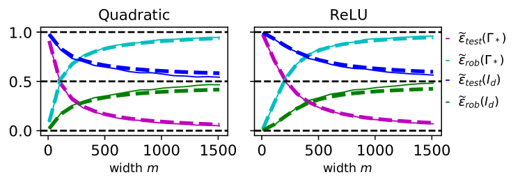
Figure 1: Empirical validation of Theorem 5.3 and Corollary 5.3. Showing (normalized) test / test error $\widetilde{\varepsilon}_{{\rm test}}$ and robustness $\widetilde{\varepsilon}_{{\rm rob}}$ of random features model (13) as a function of the number of the network width, for different choices of the covariance matrix $\Gamma$ of the random weights of the hidden neurons: the optimal choice $\Gamma_{\star}\propto B$ and the naive choice $I_{d}$. Here, the input-dimension is $d=450$ and the regularization $\lambda$ is zero. Horizontal broken lines correspond to asymptotes at $\alpha_{\infty}^{2}$ at $1-\alpha_{\infty}^{2}$, where $\alpha_{\infty}:=\lim_{d\to\infty}\mathrm{tr}(B\Gamma)/(\|B\|_{F}\|\Gamma\|_{F})$ is the level of task-alignment of the covariance matrix $\Gamma$ of hidden neurons, w.r.t learning the ground-truth function $f_{\star}$ defined in (2). Broken curves are theoretical predictions, while solid curves correspond to actual experiments.

5.3 Analysis of robustness in RF regime

The following result establishes an analytic formula for the robustness in the RF regime. [] Consider the random features model $f_{\mathrm{RF}}$ (13), with covariance matrix $\Gamma$ satisfying Condition 5.1 and activation function $\sigma$ satisfying Conditions 5.1 and 5.1.

(A) In the limit (4), we have the following approximation

$$\widetilde{\varepsilon}_{{\rm rob}}(f_{\mathrm{RF}})=\frac{\tau^{2}(2\kappa\psi_{1}^{2}+\psi_{2})}{\|B\|^{2}_{F}(2\kappa\psi_{1}+2)^{2}}+o_{d,\mathbb{P}}(1).$$ (23)

(B) If the alignment $\alpha$ admits a limit $\alpha_{\infty}$ as $d\to\infty$, then w.p $1$ it holds that

$$\lim_{\rho\to\infty}\lim\limits_{\begin{subarray}{c}m,d\to\infty\\ m/d\to\rho\end{subarray}}\widetilde{\varepsilon}_{{\rm rob}}(f_{\mathrm{RF}})=\alpha_{\infty}^{2}\leq 1.$$ (24)

In particular, for the optimal choice of $\Gamma$ in terms of test error, namely $\Gamma\propto B$, it holds w.p. $1$ that

$$\lim_{\rho\to\infty}\lim\limits_{\begin{subarray}{c}m,d\to\infty\\ m/d\to\rho\end{subarray}}\widetilde{\varepsilon}_{{\rm rob}}(f_{\mathrm{RF}})=1.$$ (25)

Thus, the robustness only depends on the aspect ratio $\rho$, the limiting spectral distribution $\mathcal{D}$ of $d\cdot\Gamma$ (via $\psi_{1}$ and $\psi_{2}$), and the scale parameters defined in (16). The theorem is proved in the Appendix D.3.

Tradeoff between approximation and robustness.

We deduce from the above theorem that in the regime (4), the random features model $f_{\mathrm{RF}}$ is more robust (i.e., stable) than the ground-truth model $f_{\star}$. Interestingly, we see that this gap in robustness between the two models closes with increasing alignment $\alpha$ between the covariance matrix of the random features $\Gamma$ and the ground-truth matrix $B$. Comparing with (22), we obtain the following relationship,

$$\widetilde{\varepsilon}_{{\rm test}}(f_{\mathrm{RF}})+\widetilde{\varepsilon}_{{\rm rob}}(f_{\mathrm{RF}})\to 1,\text{ in the limit }\eqref{eq:proportionate},$$ (26)

which trades-off between the normalized test error $\widetilde{\varepsilon}_{{\rm test}}(f_{\mathrm{RF}})$ (defined in (21)) and the normalized robustness $\widetilde{\varepsilon}_{{\rm rob}}(f_{\mathrm{RF}})$ of $f_{\mathrm{RF}}$. Thus, we have identified another novel trade-off between the test error and the robustness in random features models.

The case of quadratic activations.

We now specialize Theorem 5.3 to the case of the quadratic activation function and obtain more transparent formulae. [] Consider the random features model $f_{\mathrm{RF}}$ with covariance matrix $\Gamma$ satisfying Condition 5.1 and quadratic activation function $\sigma(t):=t^{2}-1$. Then, in the limit (4), it holds that $\widetilde{\varepsilon}_{{\rm rob}}(f_{\mathrm{RF}})=\dfrac{\mathrm{tr}(B\Gamma)^{2}\|\Gamma\|_{F}^{2}}{(2/m+\|\Gamma\|_{F}^{2})^{2}\|B\|_{F}^{2}}+o_{d,\mathbb{P}}(1).$ Furthermore, parts (B) and (C) of Theorem 5.3 hold. Theorem 5.3 and Corollary  5.3 are empirically verified in Fig. 1. Notice the perfect match between our theoretical results and experiments.

6 Neural tangent (NT) regime

Consider a two-layer network with output weights $z^{0}_{j}$ fixed to $1$, and hidden weight $w_{j}\in\mathbb{R}^{d}$ drawn from $N(0,\Gamma)$. For the quadratic activation $\sigma(t):=t^{2}$, the neural tangent (NT) approximation Jacot et al. (2018); Chizat et al. (2019) w.r.t. the first layer parameters is given by

$$f_{W+A}(x)\approx f_{\mathrm{init}}(x)+\mathrm{tr}(A\nabla_{W}f_{W}(x))=f_{\mathrm{init}}(x)+2\sum_{j=1}^{m}(x^{\top}(z^{0}_{j}a_{j}))(x^{\top}w_{j}).$$ (27)

where $f_{\mathrm{init}}$ is the function computed by the neural network at initialization (see Appendix B for details), and $A=(a_{1},\ldots,a_{m})=(\Delta w_{1},\ldots,\Delta w_{m})\in\mathbb{R}^{m\times d}$ is the change in $W$. We will see that the initialization term $f_{\mathrm{init}}$ might have drastic influence on the robustness of the resulting model.

6.1 NT approximation without initialization term

We temporarily discard the initialization term $f_{\mathrm{init}}(x)$ from the RHS of (27), and consider the simplified approximation

$$f_{\mathrm{NT}}(x;A;c):=2\sum_{j=1}^{m}(x^{\top}a_{j})(x^{\top}w_{j})-c,$$ (28)

where, without loss of generality, we absorb the output weights $z_{j}$ in the parameters $a_{j}$ in the first-order term. In (28), $A\in\mathbb{R}^{m\times d}$ and $c\in\mathbb{R}$ are model parameters that are optimized. In terms of test error, let $A_{\mathrm{NT}}$ and $c_{\mathrm{NT}}$ be optimal in $f_{\mathrm{NT}}(\cdot;A,c)$, and let $f_{\mathrm{NT}}=f_{\mathrm{NT}}(\cdot;A_{\mathrm{NT}},c_{\mathrm{NT}})$ for short. In Thm. 2 of Ghorbani et al. (2019), it is shown that the (normalized) test error of the linearized model $f_{\mathrm{NT}}$ is given by

$$\mathbb{E}_{W}[\widetilde{\varepsilon}_{{\rm test}}(f_{\mathrm{NT}})] =(1-\rho)_{+}^{2}(1-\beta)+(1-\rho)_{+}\beta+o_{d}(1).$$ (29)

where $\beta=\beta(B):=\mathrm{tr}(B)^{2}/(d\|B\|_{F}^{2})\in[0,1]$. Our objective in this section is to compute the robustness of $f_{\mathrm{NT}}$. Let $\rho:=\min(\rho,1)$.

[] $\mathfrak{S}(f_{\mathrm{NT}})^{2}=4\|W^{\top}A+A^{\top}W\|_{F}^{2}.$

Combining with Lemma 6.1 above, we can prove the following result (see appendix).

[] Consider the neural tangent model $f_{\mathrm{NT}}$ in (28). In the limit (4) it holds that,

$$\mathbb{E}_{W}[\widetilde{\varepsilon}_{{\rm rob}}(f_{\mathrm{NT}})]=\frac{\underline{\rho}+\underline{\rho}^{2}}{2}+\frac{(\underline{\rho}-\underline{\rho}^{2})\beta}{2}+o_{d}(1).$$ (30)

Further observe that because $\beta\leq 1$, the RHS of (30) is further upper-bounded by $\underline{\rho}\leq 1$ with equality when $\beta=1$ (e.g., for $B\propto I_{d}$). We deduce that in the NT regime, the neural network is at least as robust as the ground-truth model $f_{\star}$. Comparing with (29), we obtain the following tradeoff between test error and robustness, stated only for $\beta=1$ for simplicity of presentation. [] If $\beta=1$ (i.e., if $B\propto I_{d})$, then in the limit (4), it holds that

$$\mathbb{E}_{W}[\widetilde{\varepsilon}_{{\rm test}}(f_{\mathrm{NT}})+\widetilde{\varepsilon}_{{\rm rob}}(f_{\mathrm{NT}})] =1+o_{d}(1).$$ (31)

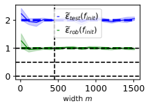
(a) NN at large random init

(b) NT regime

(c) Lazy, small random init

(d) Lazy, large random init

Figure 2: Showing curves of (normalized) test error $\widetilde{\varepsilon}_{{\rm test}}$ and robustness $\widetilde{\varepsilon}_{{\rm rob}}$ for a two-layer neural network in different learning regimes of the hidden weights. Here, the input dimension is $d=450$ and the width $m$ sweeps a range of values from $10$ to $1500$. Dashed curves correspond to theoretical predictions, while solid curves correspond to actual values observed in the experiment (5 runs). We use $n=10^{6}$ training samples as a proxy for infinite data. The covariance matrix of the hidden neurons is fixed at $\Gamma=(1/d)I_{d}$. For simplicity, simplicity of this experiment, we also take the coefficient matrix in the ground-truth function as $B\propto I_{d}$. (c) ”Small random init” means $B=(1/\sqrt{d})I_{d}$, so that $B$ is much larger than $\Gamma$. (d) ”Large random init” means that $B=(1/d)I_{d}$, and thus is of the same order as $\Gamma$ (in Frobenius norm). In this case, the initialization degrades the robustness, as predicted by Thm. 6.2. Note that, as predicted by Thm. 6.2, random initialization has no impact on the test error of the neural tangent approximation. Results for (a) the neural network at initialization (Thm. B and B) and (b) In the neural tangent regime (Thm. 6.1) are also depicted for reference.

6.2 NT approximation with initialization term

We now consider the neural tangent approximation (27) without discarding the initialization term $f_{\mathrm{init}}$ from the RHS of (27). Also, let $z^{0}\in\mathbb{R}^{m}$ be the output weights, drawn iid from $N(0,1/m)$ and frozen, and let $Q$ be the $m\times m$ diagonal matrix with $z^{0}$ as its diagonal. This corresponds to what could be referred to as lazy training regime of the hidden layer. Let $f_{\mathrm{NTL}}(x;A,c)$ be RHS of (27),

$$f_{\mathrm{NTL}}(x;A,c) :=f_{W,z,c}(x)+2\sum_{j=1}^{m}(x^{\top}w_{j})(x^{\top}a_{j})=f_{\mathrm{init}}(x)+f_{\mathrm{NT}}(x;A,c),$$ (32)

where $f_{\mathrm{init}}(x):=\sum_{j=1}^{m}z^{0}_{j}(x^{\top}w_{j})^{2}=x^{\top}W^{\top}QWx$ defines the neural network at initialization.

[] Suppose the output weights $z^{0}$ at initialization are iid from $N(0,(1/m)I_{m})$. Then, in the limit (4), the following identities hold

$$\mathbb{E}_{\{W,z^{0}\}}[\widetilde{\varepsilon}_{{\rm test}}(f_{\mathrm{NTL}})] =\mathbb{E}_{W}[\widetilde{\varepsilon}_{{\rm test}}(f_{\mathrm{NT}})]+o_{d}(1),$$ (33)

$$\mathbb{E}_{\{W,z^{0}\}}[\widetilde{\varepsilon}_{{\rm rob}}(f_{\mathrm{NTL}})] =\mathbb{E}_{W}[\widetilde{\varepsilon}_{{\rm rob}}(f_{\mathrm{NT}})]+\mathbb{E}_{\{W,z^{0}\}}[\widetilde{\varepsilon}_{{\rm rob}}(f_{\mathrm{init}})]+o_{d}(1).$$ (34)

Thus, on average (over initialization): (i) $f_{\mathrm{NTL}}$ and $f_{\mathrm{NT}}$ have the same test error, i.e., the initialization term $f_{\mathrm{init}}$ in $f_{\mathrm{NTL}}$ does not affect its test error. (ii) On the other hand, $f_{\mathrm{NTL}}$ is less robust than $f_{\mathrm{NT}}$; the deficit in robustness, namely the term $(1+\|\Gamma\|^{2})/\|B\|_{F}^{2}$, corresponds exactly to the contribution of the initialization. The situation is empirically illustrated in Fig. 2. Notice the perfect match between our theoretical results and experiments.

7 Concluding remarks

In this paper, we have studied the adversarial robustness of two-layer neural networks in different high-dimensional learning regimes, and established a number of new tradeoffs between prediction performance and robustness. Our analysis also shows that random initialization can further degrade the robustness in lazy training regimes: for ”large” random initialization, the trained neural network inherits an additional nonrobustness already present at initialization.

Our work can be seen as a first step towards a rigorous analysis of the robustness of trained neural networks, a subject which is still understudied.

Appendix A Justification of our proposed measure of robustness

Let us begin by explaining why our proposed measure of robustness based on Dirichlet energy (7) is actually a measure of robustness.

Given a continuously-differentiable function $f:\mathbb{R}^{d}\to\mathbb{R}$, consider the $d\times d$ psd matrix $J(f)$ defined by

$$J(f):=\mathbb{E}_{x\sim N(0,I_{d})}[\nabla_{x}f(x)\otimes\nabla_{x}f(x)].$$ (35)

We will see that the spectrum of this matrix plays a key role in quantifying the robustness of $f$, w.r.t the distribution $P$. The following lemma shows that $\mathfrak{S}(f)^{2}=\mathrm{tr}(J(f))$, and measures the (non)robustness of $f$ to random local fluctuations in its input. [Derivative of robustness error] We have

$$\lim_{\delta\to 0^{+}}\frac{1}{\delta}\mathbb{E}_{x\sim N(0,I_{d})}[\Delta_{f}(x;\delta)]=\mathfrak{S}(f)=\mathrm{tr}(J(f))^{1/2},$$ (36)

where $\Delta_{f}(x;\delta):=\sup_{\|v\|_{2}\leq\delta}|f(x+v)-f(x)|$. This lemma is a direct corollary to Lemma A.2 proved later below.

The next lemma shows that $\|J(f)\|_{op}$ measures the (non)robustness of $f$ to universal adversarial perturbations, in the sense of Moosavi-Dezfooli et al. (2017). [Measure of robustness to universal perturbations] We have the identity

$$\lim_{\delta\to 0^{+}}\frac{1}{\delta}\Delta_{f}(\delta)=\|J(f)\|_{op}^{1/2},$$ (37)

where $\Delta_{f}(\delta)^{2}:=\sup_{\|v\|\leq\delta}\mathbb{E}_{x\sim N(0,I_{d})}(f(x+v)-f(x))^{2}$. In particular, the leading eigenvector of $J(f)$ corresponds to (first-order) universal adversarial perturbations of $f$, in the sense of Moosavi-Dezfooli et al. (2017), which can be efficiently computed using the Power Method, for example.

A rough sketch of the proof of the above lemma is as follows. To first-order, we have $f(x+v)-f(x)\approx v^{\top}\nabla xf(x)$. Thus,

$$\begin{split}\Delta_{f}(\delta)^{2}&\approx\sup_{\|v\|\leq\delta}\mathbb{E}_{x\sim N(0,I_{d})}[(f(x+v)-f(x))^{2}]\\ &=\sup_{\|v\|\leq\delta}\mathbb{E}_{x\sim N(0,I_{d})}[(v^{\top}\nabla_{x}f(x))^{2}]\\ &=\sup_{\|v\|\leq\delta}v^{\top}J(f)v=\delta^{2}\|J(f)\|_{op}^{2}.\end{split}$$

The first lemma is proved via a similar argument.

A.1 Why not use Lipschitz constants to measure robustness ?

Note for any that smooth function $f:\mathbb{R}\to\mathbb{R}$, $\mathfrak{S}(f)$ is always a lower-bound for the Lipschitz constant $\|f\|_{\mathrm{Lip}}$ of $f$. Recall that $\|f\|_{\mathrm{Lip}}$ is defined by

$$\|f\|_{\mathrm{Lip}}:=\sup_{x\neq x^{\prime}}\frac{|f(x)-f(x^{\prime})|}{\|x-x^{\prime}\|}.$$ (38)

One special case where there is equality $\mathfrak{S}(f)=\|f\|_{\mathrm{Lip}}$ is when $f$ is a linear function. However, this is far from true in general: $\|f\|_{\mathrm{Lip}}$ is a worst-case measure, while $\mathfrak{S}(f)$ is an average-case measure for each $q$. If $\|f\|_{\mathrm{Lip}}$ is small (i.e., of order $\mathcal{O}(1)$), then a small perturbation (i.e., of size $\mathcal{O}(1)$) can only result in mild change in the output of $f$ (i.e., of order $\mathcal{O}(1)$). However, a large value of $\|f\|_{\mathrm{Lip}}$ is uninformative regarding adversarial examples (for example, one can think of a function which is smooth everywhere except on a set of measure zero). In contrast, a large value for $\mathfrak{S}(f)$ indicates that, on average, it is possible for an adversarial to drastically change the output of $f$ via a small modification of its input.

An illustrative example.

Consider a quadratic function $f(x):=(1/2)x^{\top}Bx+c$. Note that the ground-truth model $f_{\star}$ defined in (2) is of this form. A direct computation reveals that $\nabla_{x}f(x)=Bx$ and so $\mathfrak{S}(f)^{2}:=\mathbb{E}_{x\sim N(0,I_{d})}\|\nabla_{x}f(x)\|^{2}=\mathbb{E}_{x\sim N(0,I_{d})}\|Bx\|^{2}=\|B\|_{F}^{2}$. However, the Lipschitz constant of $f$ restricted to the ball of radius $\sqrt{d}$ is,

$$\|f\|_{\widetilde{\mathrm{Lip}}}=\underset{\|x\|\leq\sqrt{d}}{\sup}\|\nabla_{x}f(x)\|=\underset{\|x\|\leq\sqrt{d}}{\sup}\|Bx\|=\sqrt{d}\|B\|_{op},$$

which can be drastically larger than $\mathfrak{S}(f)=\|B\|_{F}$. For example, take $B$ to be an ill-conditioned, e.g., rank-$1$, matrix.

A.2 Proofs for Dirichlet energy as a measure of adversarial vulnerability

Let $P$ be a probability distribution on $\mathbb{R}^{d}$, for example, the gaussian distribution $N(0,I_{d})$ assumed in the main article. Let $\|\cdot\|$ be any norm on $\mathbb{R}^{d}$ with dual norm $\|\cdot\|_{\star}$. Given a function $f:\mathbb{R}^{d}\to\mathbb{R}$, a tolerance parameter $\delta\geq 0$ (the attack budget), and a scalar $q\geq 1$, define $R_{\delta}(f)$ by

$$R_{q,\delta}(f,g):=\mathbb{E}_{x\sim P}\left[\Delta_{f}(x;\delta)^{q}\right],$$ (39)

where $\Delta_{f}(x;\delta):=\sup_{\|x^{\prime}-x\|\leq\delta}|f(x^{\prime})-f(x)|$ is the maximal variation of $f$ in a neighborhood of size $\delta$ around $x$. For $q=2$, we simply write $R_{\delta}(f,g)$ for $R_{\delta,2}(f,g)$. In particular, $G_{\delta}(f):=\mathbb{E}[R_{\delta}(f,f_{\star})]$ is adversarial test error and $G_{0}(f):=\mathbb{E}[R_{0}(f,f_{\star})]$ is the ordinary test error of $f$, where the expectations are w.r.t all sources of randomness in $f$ and $f_{\star}$. Of course $G_{\delta}(f)$ is an increasing function of $\delta$.

Define $R_{q,\delta}(f):=R_{q,\delta}(f,f)$ and $R_{\delta}(f):=R_{2,\delta}(f,f)$, which measure the deviation of the outputs of $f$ w.r.t to the outputs of $f$, under adversarial attack. Note $R_{q}(f)\equiv 0$. Also note that in the case where $\|\cdot\|$ is the euclidean $L_{2}$-norm: if $f$ is a near perfect model (in the classical sense), meaning that its ordinary test error $G_{0}(f)$ is small, then $R_{\delta}(f)$ is a good approximation for $G_{\delta}(f)$. Finally, (at least for small values of $\alpha$), we can further approximate $R_{\alpha}(f)$ (and therefore $G_{\delta}(f)$, for near perfect $f$) by $\delta^{2}$ times the Dirichlet energy $\mathfrak{S}(f)^{2}$. Indeed, [] Suppose $f$ is $P$-a.e differentiable and for any $q\in[1,\infty)$, define $\mathfrak{S}_{q}(f)$ by

$$\begin{split}\mathfrak{S}_{q}(f)&:=\left(\mathbb{E}_{x\sim P}[\|\nabla_{x}f(x)\|_{\star}^{q}]\right)^{1/q}.\end{split}$$ (40)

(In particular, if $\|\cdot\|$ is the euclidean $L_{2}$-norm and $q=2$, then $\mathfrak{S}_{q}(f)^{2}$ is the Dirichlet energy defined in (7) as our measure of robustness). We have the following

(A) General case. $\mathfrak{S}_{q}(f)$ is the right derivative of the mapping $\delta\mapsto R_{\delta}(f)^{1/q}$ at $\delta=0$. More precisely, we have the following

$$\lim_{\delta\to 0^{+}}\frac{R_{q,\delta}(f)^{1/q}}{\delta}=\mathfrak{S}_{q}(f),$$ (41)

or equivalently, $R_{q,\delta}(f)=\delta^{q}\cdot\mathfrak{S}_{P}(f)^{q}+\text{ Higher order terms in }\delta^{q}$.

(B) Case of Dirichlet energy In particular, if $\|\cdot\|$ is the euclidean $L_{2}$-norm, and we take $q=2$,

$$R_{\delta}(f)=\delta^{2}\cdot\mathfrak{S}_{P}(f)^{2}+\text{ Higher order terms in }\delta^{2}.$$ (42)

[] A heuristic argument was used in Simon-Gabriel et al. (2019) to justify the use of average (dual-)norm of gradient (i.e the average local Lipschitz constant) $\mathbb{E}_{x\sim N(0,I_{d})}[\|\nabla_{x}f(x)\|_{\star}]$ (corresponding to $q=1$ in the above) as a proxy for the adversarial generalization.

The proof of Lemma A.2 follows directly Fubini’s Theorem and the following lemma. [] If $f$ is differentiable at $x$, then the function $\delta\mapsto\Delta_{f}(x;\delta):=\underset{\|x^{\prime}-x\|\leq\delta}{\sup}|f(x^{\prime})-f(x)|$ is right-differentiable at $0$ with derivative given by $\Delta_{f}^{\prime}(x;0)=\|\nabla_{x}f(x)\|_{\star}$.

Proof.

As $f$ is differentiable, $f(x^{\prime})=f(x)+\nabla_{x}f(x)^{\top}(x^{\prime}-x)+o(\|x^{\prime}-x\|)$ around $x$. Therefore for sufficiently small $\delta$, if $B(x;\delta)$ is ball of radius $\delta$ around $x$, then

$$\begin{split}\Delta_{f}(x;\delta)&=\sup_{x^{\prime}\in B(x;\delta)}\mid\nabla_{x}f(x)^{\top}(x^{\prime}-x)+o(\|x^{\prime}-x\|)\mid\\ &\leq\sup_{x^{\prime}\in B(x;\delta)}|\nabla_{x}f(x)^{\top}(x^{\prime}-x)|+\sup_{y\in B(x;\delta)}o(\|x^{\prime}-x\|)\\ &=\|\nabla_{x}f(x)\|_{\star}\delta+\sup_{y\in B(x;\delta)}o(\|x^{\prime}-x\|)\frac{\Delta_{f}(x;\delta)}{\delta}\\ &\leq\|\nabla_{x}f(x)\|_{\star}+\sup_{x^{\prime}\in B(x;\delta)}\frac{o(\|x^{\prime}-x\|)}{\delta}\end{split}$$ (43)

Note that $\sup_{x^{\prime}\in B(x;\delta)}\dfrac{o(\|x^{\prime}-x\|)}{\delta}\rightarrow 0$. This proves $\limsup_{\delta\to 0^{+}}(1/\delta)\Delta_{f}(x;\delta)\leq\|\nabla_{x}f(x)\|_{\star}$. Similarly, one computes

$$\begin{split}\Delta_{f}(x;\delta)&=\sup\mid\nabla_{x}f(x)^{\top}(x^{\prime}-x)+o(\|x^{\prime}-x\|)\mid\\ &\geq\sup|\nabla_{x}f(x)^{\top}(x^{\prime}-x)|-\sup o(\|x^{\prime}-x\|)\\ &=\|\nabla_{x}f(x)\|\delta-\sup o(\|x^{\prime}-x\|)\end{split}$$ (44)

Hence $\liminf_{\delta\to 0^{+}}(1/\delta)\Delta_{f}(x;\delta)\geq\|\nabla_{x}f(x)\|_{\star}$, and we conclude that $\delta\mapsto\Delta_{f}(x;\delta)$ is differentiable at $\delta=0$, with derivative $\Delta_{f}^{\prime}(x;0)=\|\nabla_{x}f(x)\|_{\star}$ as claimed. ∎

Proof of Lemma A.2.

By basic properties of limits, one has

$$\begin{split}\left(\lim_{\delta\to 0^{+}}\frac{R_{q,\delta}(f)^{1/q}}{\delta^{q}}\right)^{q}&=\lim_{\delta\to 0^{+}}\frac{R_{q,\delta}(f)}{\delta}\\ &=\lim_{\delta\to 0^{+}}\frac{\mathbb{E}_{x\sim P}[|\Delta_{f}(x;\delta)|^{q}]}{\delta}\\ &=\mathbb{E}_{x\sim P}\left[\lim_{\delta\to 0^{+}}\frac{|\Delta_{f}(x;\delta)|^{q}}{\delta}\right]\\ &=\mathbb{E}_{x\sim P}\left[\left(\lim_{\delta\to 0^{+}}\frac{|\Delta_{f}(x;\delta)|}{\delta}\right)^{q}\right]\\ &=\mathbb{E}_{x\sim P}[\|\nabla_{x}f(x)\|_{\star}^{q}]\\ &:=\mathfrak{S}_{q}(f)^{q},\end{split}$$ (45)

where the 3rd line is thanks to Fubini’s Theorem, and the 5th line is thanks to lemma A.2 (and the fact that $\Delta_{f}(x;0)\equiv 0$). Noting that $R_{q,0}(f)\equiv 0$ then concludes the proof. ∎

Appendix B Neural networks at (random) initialization

We now consider networks at initialization, wherein the hidden weights matrix $W=(w_{1},\ldots,w_{m})$ is a random $m\times d$ matrix with iid rows from $N(0,\Gamma)$ as in the random features regime (13), but we freeze the output weight vector $z=z_{0}\in\mathbb{R}^{m}$ at random initialization, with random iid entries from  $N(0,1/m)$, following standard initialization procedures. Let  $f_{\mathrm{init}}$ denote this random network, i.e.,

$$f_{\mathrm{init}}(x):=(z^{0})^{\top}\sigma(Wx)=\sum_{j=1}^{m}z^{0}_{j}\sigma(x^{\top}w_{j}).$$ (46)

[] Under the Conditions 5.1 and 5.1, we have the identity in the limit (4),

$\widetilde{\varepsilon}_{{\rm rob}}(f_{\mathrm{init}})=\dfrac{\|\sigma^{\prime}\|^{2}_{L^{2}(N(0,1))}+\lambda_{3}^{2}\|\Gamma\|_{F}^{2}/2+\lambda_{2}^{2}\|\Gamma\|_{F}^{2}}{4\|B\|_{F}^{2}}+o_{d,\mathbb{P}}(1),$ where $\lambda_{k}$ is the $k$th Hermite coefficient of the activation function $\sigma$. In particular, for the quadratic activation function $\sigma(t)=t^{2}-1$, we have $\widetilde{\varepsilon}_{{\rm rob}}(f_{\mathrm{init}})=\dfrac{1+\|\Gamma\|^{2}_{F}}{\|B\|^{2}_{F}}+o_{d,\mathbb{P}}(1).$ Analogously, the test error for the NN at initialization is given by the following result. [] Under the Conditions 5.1 and 5.1, we have the following identity in the limit (4), $\widetilde{\varepsilon}_{{\rm test}}(f_{\mathrm{init}})=1+\dfrac{\|\sigma\|^{2}_{L^{2}(N(0,1))}+\lambda_{2}^{2}\|\Gamma\|_{F}^{2}/2}{2\|B\|_{F}^{2}}+o_{d,\mathbb{P}}(1).$ In particular, for the quadratic activation $\sigma(t):=t^{2}-1$, we have the following identity $\widetilde{\varepsilon}_{{\rm test}}(f_{\mathrm{init}})=1+\dfrac{1+\|\Gamma\|_{F}^{2}}{\|B\|_{F}^{2}}+o_{d,\mathbb{P}}(1).$

Combining Thm. B with formula (11), we deduce that training a randomly initialized neural network always improves its test error, as one would expect. On the other hand, combining Thm. 4 and Thm. B, we deduce that fully training the networks (10) via SGD:

(1) Degrades robustness if $\|B\|_{F}^{2}\gtrsim\|\Gamma\|_{F}^{2}+1$. This is because in this case, the parameters of the model align to the signal matrix $B$, which has much larger energy than the parameters at initialization. Indeed, SGD tends to move the covariance structure of the hidden neurons from $\Gamma$ to $B$.

(2) Improves robustness if $\|B\|_{F}^{2}\lesssim\|\Gamma\|_{F}^{2}+1$.

Appendix C Miscellaneous

C.1 Lazy training of output layer in RF regime

We now study the influence of the initialization on the random features regime. Let $W=(w_{1},\ldots,w_{m})\in\mathbb{R}^{m\times d}$ with random rows drawn iid from $N(0,\Gamma)$ as in the RF model (13), and let the output layer be initialized at $z=z^{0}\sim N(0,(1/m)I_{d})$ and updated via single-pass gradient-flow on the entire data distribution (infinite data). In this so-called random features lazy (RFL) regime, we posit the following approximation neural network (3)

$$f_{\mathrm{RFL}}(x):=z_{\mathrm{RFL},\lambda}^{\top}\sigma(Wx)=f_{\mathrm{init}}(x)+\delta_{\lambda}^{\top}\sigma(Wx),$$ (47)

where $z_{\mathrm{RFL},\lambda}:=z^{0}+\delta_{\lambda}$ and $\delta_{\lambda}\in\mathbb{R}^{m}$ solves the following ridge-regression problem

$$\begin{split}\arg\min_{\delta\in\mathbb{R}^{m}}\mathbb{E}_{x\sim N(0,I_{d})}[(\delta^{\top}\sigma(Wx)+f_{\mathrm{init}}(x)-f_{\star}(x))^{2}]+\lambda\|\delta\|^{2}.\end{split}$$ (48)

The use of the ridge parameter here can be thought of as a proxy for early-stopping at iteration $t\propto 1/\lambda$ Ali et al. (2020); $\lambda=0$ corresponds to training the output layer to optimality.

[] We have the following identities

$$\mathbb{E}_{z^{0}}[\widetilde{\varepsilon}_{{\rm test}}(f_{\mathrm{RFL},\lambda})] =\widetilde{\varepsilon}_{{\rm test}}(f_{\mathrm{RF}})+\frac{\mathrm{tr}(P_{\lambda}^{2}U)/m}{2\|B\|_{F}^{2}}+o_{d,\mathbb{P}}(1)$$ (49)

$$\mathbb{E}_{z^{0}}[\widetilde{\varepsilon}_{{\rm rob}}(f_{\mathrm{RFL},\lambda})] =\widetilde{\varepsilon}_{{\rm rob}}(f_{\mathrm{RF}})+\frac{\mathrm{tr}(P_{\lambda}^{2}C)/m}{4\|B\|_{F}^{2}}+o_{d,\mathbb{P}}(1),$$ (50)

where $U=U(W)$ and $C=C(W)$ are the random matrices defined in (17) and (9) respectively. Because $P_{\lambda}^{2}$, $U$, and $C$ are psd matrices, the residual terms $\mathrm{tr}(P_{\lambda}^{2}U)/m$ and $\mathrm{tr}(P_{\lambda}^{2}C)/m$ in the above formulae are nonnegative. We deduce that random initialization of the output weights hurts both test error and robustness, as long as the RFL regime is valid.

Infinitely regularized case $\lambda\to\infty$. Note that $P_{\lambda}$ converges in spectral norm a.s to the identity matrix $I_{m}$ in the limit $\lambda\to\infty$. Thus, in this limit, $z_{\mathrm{RF},\lambda}$ converges almost-surely to the all-zero $m$-dimensional vector and so, thanks to (88), the output weights $z_{\mathrm{RFL},\lambda}$ of $f_{\mathrm{RFL},\lambda}$ converge to the value at initialization $z^{0}$. Therefore, $f_{\mathrm{RFL},\lambda}$ and all its derivatives converge a.s point-wise its state $f_{\mathrm{init}}$ at initialization (46). We deduce that in the $\lambda\to\infty$ limit, the neural network in the lazy regime is equivalent to an untrained model $f_{\mathrm{init}}$, in terms of test error and robustness. This does not come as much of a surprise, since $\lambda\to\infty$, corresponds to early-stopping at $t=0$, i.e., no optimization.

Unregularized case $\lambda\to 0^{+}$. By an analogous argument as above, $P_{\lambda}$ converges a.s. to the all-zero $m\times m$ matrix in the limit $\lambda\to 0^{+}$, and so thanks to (88), we have the almost-sure convergence $\|z_{\mathrm{RFL},\lambda}-z_{\mathrm{RF},\lambda}\|\to 0$. We deduce that in this limit, the unregularized lazy training regime is exactly equivalent to the unregularized vanilla RF regime. Thus, the random features lazy (RFL) regime corresponding to the approximation $f_{\mathrm{RFL}}$ is an interpolation between the random features regime (corresponding to $f_{\mathrm{RF}}$) and the untrained regime (corresponding to $f_{\mathrm{init}}$).

Although this is not useful in our infinite data regime, we remark that a non-zero amount of regularization is often crucial for good statistical performance with finite samples. In this, case, $P_{\lambda}$ is non-zero, and we expect both the test error and robustness to become worse in this lazy RF approximation, compared to vanilla RF.

C.2 Effect of regularization in RF regime

Suppose the estimation of the output weights of the RF model is regularized, i.e., for a fixed $\lambda\geq 0$, consider instead the model $f_{\mathrm{RF},\lambda}(x):=z_{\mathrm{RF},\lambda}^{\top}\sigma(Wx)$, where $z_{\mathrm{RF},\lambda}$ is chosen to solve the following ridge-regularized problem

$$\min_{z\in\mathbb{R}^{m}}\|f_{W,z}-f_{\star}\|_{L^{2}(N(0,I_{d}))}^{2}+\lambda\|z\|^{2}.$$ (51)

A simple computation gives the explicit form

$$z_{\mathrm{RF},\lambda}=U_{\lambda}^{-1}v,$$ (52)

where $U_{\lambda}:=U+\lambda I_{m}$, $U=U(W)$ is the random matrix defined in (17), and $v\in\mathbb{R}^{m}$ is random vector defined in (18). An inspection of the proof of Theorem 5.3 (see Appendix D.3) reveals that the situation in the presence of ridge regularization is equivalent to the unregularized case in which we replace $\overline{\lambda}$ by $\overline{\lambda}+\lambda$ in the definition of the matrix $A_{0}$ which appears in (20). This has the effect of decreasing $\psi_{1}$ and $\psi_{2}$, and thanks to (23), decreasing the robustness of the random features model. That is, $\widetilde{\varepsilon}_{{\rm rob}}(f_{\mathrm{RF},\lambda})$ is a decreasing function of the amount of regularization of $\lambda$, and in fact, $\underset{\lambda\to\infty}{\lim}\,\widetilde{\varepsilon}_{{\rm rob}}(f_{\mathrm{RF},\lambda})=0$.

Appendix D Technical proofs

Before proving the main results of the manuscript, we first state and prove some auxiliary results which will be instrumental.

D.1 Proof of Lemma 3.4: generic formula for (non)robustness of neural network

Recall the definitions of the approximation error and robustness metrics from Section 3.4. The following lemma was used to express the measure of (non)robustness $\mathfrak{S}(f_{w,z})^{2}$ of a two-layer neural network $f_{w,z}$ as a quadratic form in the output weights, with coefficient matrix which depends on the distribution of the hidden weights. See 3.4

Proof.

One direcly computes $\nabla_{x}f_{W,z}(x)=\sum_{j=1}^{m}z_{j}\sigma^{\prime}(x^{\top}w_{j})w_{j}$, and so the Laplacian of $f_{W,z}$ at $x$ is given by

$$\|\nabla_{x}f_{W,z}(x)\|^{2}=\sum_{j,k=1}^{m}z_{j}z_{k}(w_{j}^{\top}w_{k})\sigma^{\prime}(x^{\top}w_{j})\sigma^{\prime}(x^{\top}w_{k}).$$ (53)

Thus, $\mathfrak{S}(f_{W,z})^{2}$ evaluates to

$$\begin{split}\mathfrak{S}(f_{W,z})^{2}&:=\mathbb{E}_{x\sim N(0,I_{d})}\|\nabla_{x}f_{W,z}(x)\|^{2}=\sum_{j,k=1}^{m}z_{j}z_{k}(w_{j}^{\top}w_{k})\mathbb{E}_{x}[\sigma^{\prime}(x^{\top}w_{j})\sigma^{\prime}(x^{\top}w_{k})]=z^{\top}C(W)z,\end{split}$$

where the $m\times m$ psd matrix $C(W)$ is as defined in Lemma 3.4. In particular, for the activation function $\sigma(t):=t^{2}+s$, one computes

$$\begin{split}c_{j,k}&:=(w_{j}^{\top}w_{k})\mathbb{E}_{x\sim N(0,I_{d})}[\sigma^{\prime}(x^{\top}w_{j})\sigma^{\prime}(x^{\top}w_{k})]\\ &=4(w_{j}^{\top}w_{k})\mathbb{E}_{x\sim N(0,I_{d})}[(x^{\top}w_{j})(x^{\top}w_{k})]=4(w_{j}^{\top}w_{k})^{2},\end{split}$$

where the last step is due to the fact that

$$\begin{split}\mathbb{E}_{x\sim N(0,I_{d})}[(x^{\top}w_{j})(x^{\top}w_{k})]&=\mathbb{E}_{x}[x^{\top}w_{j}w_{k}^{\top}x]=\mathrm{tr}(\mathrm{Cov}(x)w_{j}w_{k}^{\top})=w_{j}^{\top}w_{k},\end{split}$$

by a standard result on the mean of a quadratic form. ∎

[Robustness of ground-truth model] It holds that $\mathfrak{S}(f_{\star})^{2}=4\|B\|_{F}^{2}$.

Proof.

For the first part follows directly from Lemma 3.4 with activation function $\sigma(t):=t^{2}+b_{0}/d$ and fixed output weight vector $a=1_{m}:=(1,\ldots,1)$. ∎

D.2 Approximation of random matrices

This section establishes some technical results for ”linearizing” a number of complicated random matrices which occur in our analysis. We will make heavy use of random matrix theory (RMT) techniques developed in Silverstein & Choi (1995); El Karoui (2010); Ledoit & Péché (2011); Dobriban & Wager (2018)

We begin by recalling the following definition for future reference. See 5.1

Let $U$ be the random $m\times m$ psd matrix defined in (17) and let $v\in\mathbb{R}^{m}$ be the random vector defined in (18). Recall that $\lambda_{k}=\lambda_{k}(\sigma)$ is the $k$ Hermite coefficient of the activation function $\sigma$. Also recall the definition of the scalars $\overline{\lambda}$, $\kappa$, $\tau$, $\overline{\lambda^{\prime}}$, and $\kappa^{\prime}$ from (16). The following result was established in Ghorbani et al. (2019). [Lemma 2 of Ghorbani et al. (2019)] If $\lambda_{0}=0$ and Conditions 5.1, 5.1 are in place, then in the limit (4), it holds that

$$\|U-U_{0}\|_{op} =o_{d,\mathbb{P}}(1),$$ (54)

$$\|v-(\tau/\sqrt{d})1_{m}\| =o_{d,\mathbb{P}}(1),$$ (55)

where the random $m\times m$ psd matrix $U_{0}$ is defined by

$$U_{0}:=\overline{\lambda}I_{m}+\lambda_{1}^{2}WW^{\top}+(\kappa/d)1_{m}1_{m}^{\top}+\mu\mu^{\top},$$ (56)

and $\mu=(\mu_{1},\ldots,\mu_{m})\in\mathbb{R}^{m}$ with $\mu_{i}:=\lambda_{2}\cdot(\|w_{i}\|^{2}-1)/2$.

A careful inspection of the proof of the estimate (54) reveals that we can remove the condition $\lambda_{0}=0$, at the expense of incurring rank-$1$ perturbations in the matrix $U_{0}$. Indeed, let us rewrite $\sigma=\overline{\sigma}+\lambda_{0}$, and with $\lambda_{0}(G)=\mathbb{E}_{G}[\overline{\sigma}(G)]=0$ with $G\sim N(0,1)$ independent of the $w_{i}$’s. Let $T_{0}$ be the $m\times m$ matrix with entries $(T_{0})_{ij}:=\lambda_{0}(\sigma_{i})\lambda_{0}(\sigma_{j})$, where $\sigma_{i}$ is the function defined by $\sigma_{i}(z):=\sigma(\|w_{i}\|z)=\overline{\sigma}_{i}(z)+\lambda_{0}$, with $\overline{\sigma}(\|w_{i}\|z):=\overline{\sigma}(\|w_{i}\|z)$. Thus, we have the decomposition

$$T_{0}=\overline{T}_{0}+\lambda_{0}(u1_{m}^{\top}+1_{m}u^{\top})+\lambda_{0}^{2}1_{m}1_{m}^{\top},$$ (57)

where $u=(\lambda_{0}(\overline{\sigma}_{i}))_{i\in[m]}$. Let $\overline{T}_{0}$ be the $m\times m$ psd matrix with entries $(\overline{T}_{0})_{ij}:=\lambda_{0}(\overline{\sigma}_{i})\lambda_{0}(\overline{\sigma}_{j})$. Using the arguments from Ghorbani et al. (2019) (since $\lambda_{0}(\overline{\sigma})=0$), one has

$$\|\overline{T}_{0}-\mu\mu^{\top}\|_{op}=o_{d,\mathbb{P}}(1).$$ (58)

Furthermore, observe that one can write $u1_{m}^{\top}=R\mu 1_{m}^{\top}$, where $R$ is the $m\times m$ diagonal matrix with $R_{ii}:=\lambda_{0}(\overline{\sigma}_{i})/\mu_{i}$. Now, for large $d$ and any $i\in[m]$, one computes

$$\begin{split}R_{ii}=\mathbb{E}_{G}\left[\frac{\sigma(\|w_{i}\|G)-\sigma(G)}{\lambda_{2}\cdot(\|w_{i}\|^{2}-1)/2}\right]&=\mathbb{E}_{G}\left[\frac{\sigma(\|w_{i}\|G)-\sigma(G)}{\|w_{i}\|-1}\right]\cdot\frac{1}{\lambda_{2}\cdot(\|w_{i}\|+1)/2}\\ &\to\frac{\mathbb{E}_{G}[G\sigma^{\prime}(G)]}{\lambda_{2}\cdot 2/2}=\frac{\lambda_{2}}{\lambda_{2}}=1.\end{split}$$ (59)

We deduce that $\|R-I_{m}\|_{op}=o_{d,\mathbb{P}}(1)$, and so $\|u1_{m}^{\top}-\mu 1_{m}^{\top}\|_{op}=o_{d,\mathbb{P}}(1)$. This proves the following extension of the above lemma which will be crucial in the sequel. [Linearization of $U$ without the Condition $\lambda_{0}(\sigma)\neq 0$] Suppose Conditions 5.1 and 5.1 are in place. In the limit (4), it holds that

$$\begin{split}\|U-\widetilde{U}_{0}\|_{op}&=o_{d,\mathbb{P}}(1),\end{split}$$ (60)

where $\widetilde{U}_{0}$ is the $m\times m$ random psd matrix given by

$$\widetilde{U}_{0}:=\widetilde{\lambda}I_{m}+\lambda_{1}^{2}WW^{\top}+(\kappa/d)1_{m}1_{m}^{\top}+\widetilde{\mu}\widetilde{\mu}^{\top},$$ (61)

with $\widetilde{\mu}:=\mu+\lambda_{0}1_{m}$ and $\widetilde{\lambda}:=\overline{\lambda}-\lambda_{0}^{2}=\mathbb{E}_{G\sim N(0,1)}[\sigma(G)^{2}]-\lambda_{0}^{2}-\lambda_{1}^{2}$.

Let $C=C(W)$ be the random $m\times m$ psd matrix with entries given by

$$c_{ij}:=(w_{i}^{\top}w_{j})\mathbb{E}_{x\sim N(0,I_{d})}[\sigma^{\prime}(x^{\top}w_{i})\sigma^{\prime}(x^{\top}w_{j})].$$ (62)

Thanks to Lemma 3.4, we know that $\mathfrak{S}(f_{\mathrm{RF}})^{2}=z_{\mathrm{RF}}^{\top}Cz_{\mathrm{RF}}=v^{\top}U^{-1}CU^{-1}v$, a random quadratic form in $v$. We start by linearizing the nonlinear random coefficient matrix $C$. [Linearization of $C$] Suppose Conditions 5.1 and 5.1 are in place. Then, in the limit (4), we have the following approximation

$$\|C-C_{0}\|_{op}=o_{d,\mathbb{P}}(1),$$ (63)

where $C_{0}$ is the $m\times m$ random psd matrix given by

$$\begin{split}C_{0}&:=\overline{\lambda^{\prime}}I_{m}+(\kappa^{\prime}/d+\lambda_{1}^{2})WW^{\top}+(2\kappa/d)1_{m}1_{m}^{\top},\end{split}$$ (64)

with $\kappa^{\prime}:=d\cdot\lambda_{3}^{2}\|\Gamma\|_{F}^{2}/2\geq 0$, and $\overline{\lambda^{\prime}}:=\|\sigma^{\prime}\|_{L^{2}(N(0,1))}^{2}-\lambda_{1}^{2}$.

Proof.

Note that $C=(WW^{\top})\odot U^{\prime}$, where $U^{\prime}$ is the $m\times m$ random psd matrix with entries given by $U^{\prime}_{ij}:=\mathbb{E}_{x\sim N(0,I_{m})}[\sigma^{\prime}(x^{\top}w_{i})\sigma^{\prime}(x^{\top}w_{j})]$.

– Step 1: Linearization. Invoking the previous lemma with $\sigma^{\prime}$ in place of $\sigma$, we know that

$$\|U^{\prime}-U_{0}^{\prime}\|_{op}=o_{d,\mathbb{P}}(1),$$ (65)

where $U^{\prime}_{0}$ is the $m\times m$ random matrix given by

$$\begin{split}U_{0}^{\prime}&:=\lambda^{\prime}I_{m}+\lambda_{1}(\sigma^{\prime})^{2}WW^{\top}+(\kappa(\sigma^{\prime})/d)1_{m}1_{m}^{\top}+(\mu+\lambda_{0}(\sigma^{\prime})1_{m})(\mu+\lambda_{0}(\sigma^{\prime})1_{m})^{\top}\\ &=\lambda^{\prime}I_{m}+\lambda_{2}(\sigma)^{2}WW^{\top}+(\kappa^{\prime}/d)1_{m}1_{m}^{\top}+(\mu+\lambda_{1}(\sigma)1_{m})(\mu+\lambda_{1}(\sigma)1_{m})^{\top},\end{split}$$ (66)

and we have used the fact that

$$\lambda_{0}((\sigma^{\prime})^{2})-\lambda_{0}(\sigma^{\prime})^{2}-\lambda_{1}(\sigma^{\prime})^{2}=\lambda_{0}((\sigma^{\prime})^{2})-\lambda_{1}(\sigma)^{2}-\lambda_{2}(\sigma)^{2}=\overline{\lambda^{\prime}}-\lambda_{2}(\sigma)^{2}=:\overline{\lambda^{\prime}}.$$

Now, since $\|WW^{\top}\|_{op}=\mathcal{O}_{d,\mathbb{P}}(1)$ by standard RMT, we deduce that from (65) that,

$$\begin{split}\|C-(WW^{\top})\odot U^{\prime}\|_{op}&=\|(WW^{\top})\odot(U^{\prime}-U_{0}^{\prime})\|_{op}\\ &\leq\|WW^{\top}\|_{op}\cdot\|U^{\prime}-U_{0}^{\prime}\|_{op}\\ &=o_{d,\mathbb{P}}(1).\end{split}$$ (67)

– Step 2: Simplification. Let $E:=\mathrm{diag}((\|w_{i}\|^{2})_{i\in[m]})$ and $F:=(WW^{\top})\odot(WW^{\top})$. Then

$$\begin{split}(WW^{\top})\odot U^{\prime}_{0}&=\lambda^{\prime}E+\lambda_{2}(\sigma)^{2}F+(\kappa^{\prime}/d)WW^{\top}+2\lambda_{1}(\sigma)\mathrm{diag}(\mu)WW^{\top}+\lambda_{1}(\sigma)^{2}WW^{\top}\\ &=\lambda^{\prime}E+\lambda_{1}(\sigma)^{2}F+(\kappa^{\prime}/d+\lambda_{1}(\sigma)^{2})WW^{\top}+2\lambda_{1}(\sigma)\mathrm{diag}(\mu)WW^{\top}.\end{split}$$ (68)

Further, because $\max_{i\in[n]}|\|w_{i}\|^{2}-1|=o_{d,\mathbb{P}}(1)$ by basic concentration, we have

$$\begin{split}\|E-I_{m}\|_{op},\|\mathrm{diag}(\mu)\|_{op}=o_{d,\mathbb{P}}(1).\end{split}$$ (69)

Also, thanks to (El Karoui, 2010, Theorem 2.3), we may linearize $F$ like so

$$\|F-(I_{m}+\|\Gamma\|_{F}^{2}1_{m}1_{m}^{\top})\|_{op}=o_{d,\mathbb{P}}(1).$$ (70)

Combining with (68) gives (recalling that $\kappa:=d\cdot\lambda_{2}(\sigma)^{2}\|\Gamma\|_{F}^{2}/2$)

$$\begin{split}(WW^{\top})\odot U^{\prime}&=(\lambda^{\prime}+\lambda_{2}(\sigma)^{2})I_{m}+(\kappa^{\prime}/d+\lambda_{1}(\sigma)^{2})WW^{\top}+(2\kappa/d)1_{m}1_{m}^{\top}+\Delta\\ &=\overline{\lambda^{\prime}}I_{m}+(\kappa^{\prime}/d+\lambda_{1}(\sigma)^{2})WW^{\top}+(2\kappa/d)1_{m}1_{m}^{\top}+\Delta\\ &=C_{0}+\Delta,\end{split}$$ (71)

where $\|\Delta\|_{op}=o_{d,\mathbb{P}}(1)$. ∎

Let us rewrite $U_{0}=A_{1}+\mu\mu^{\top}$ and $C_{0}=D_{0}+(2\kappa/d)1_{m}1_{m}^{\top}$, where

$$\begin{split}A_{1}&:=A_{0}+(\kappa/d)1_{m}1_{m}^{\top},\\ A_{0}&:=\widetilde{\lambda}I_{m}+\lambda_{1}^{2}WW^{\top},\\ D_{0}&:=\overline{\lambda^{\prime}}I_{m}+(\kappa^{\prime}/d+\lambda_{1}^{2})WW^{\top}.\end{split}$$ (72)

We will need the following lemmas. [] We have the following approximation

$$\begin{split}\mathfrak{S}(f_{\mathrm{RF}})^{2}&=u^{\top}C_{0}u+o_{d,\mathbb{P}}(1)\\ &=\tau^{2}\frac{1_{m}^{\top}U_{0}^{-1}C_{0}U_{0}^{-1}1_{m}}{d}+o_{d,\mathbb{P}}(1),\end{split}$$ (73)

where $u:=U_{0}^{-1}h$, with $h:=(\tau/\sqrt{d})1_{m}=\lambda_{2}\cdot\mathrm{tr}(B\Gamma)1_{m}$ and $U_{0}$ is defined as in Proposition D.2 and $C_{0}$ is as defined in Lemma D.2.

Proof.

Thanks to Proposition D.2, the fitted output weights vector $z_{\mathrm{RF}}\in\mathbb{R}^{m}$ concentrates around $u:=U_{0}^{-1}h$. On the other hand, we know from Lemma 3.4 that $\mathfrak{S}(f_{\mathrm{RF}})^{2}=z_{\mathrm{RF}}^{\top}Cz_{\mathrm{RF}}$. The result then follows from Lemma D.2. ∎

[] Under Condition 5.1, the following holds in the limit (4)

$$\frac{1_{m}^{\top}U_{0}^{-1}1_{m}}{d} =\frac{\psi_{1}}{1+\kappa\psi_{1}}+o_{d,\mathbb{P}}(1),$$ (74)

$$\frac{1_{m}^{\top}A_{1}^{-1}\mu}{\sqrt{d}} =o_{d,\mathbb{P}}(1),$$ (75)

$$\|A_{1}^{-1}\|_{op},\|D_{0}\|_{op} =\mathcal{O}_{d,\mathbb{P}}(1).$$ (76)

where $\psi_{1}>0$ is as defined in (20).

Proof.

Formula (74) was established in the proof of (Ghorbani et al., 2019, Theorem 1), whilst (75) was established in the proof of Lemma 5 of the same paper.

As for (76), we note that

$$\|A_{1}^{-1}\|_{op}=\|(\overline{\lambda}I_{m}+\lambda_{1}^{2}WW^{\top})^{-1}\|_{op}=\mathcal{O}_{d,\mathbb{P}}(1/\overline{\lambda},\lambda_{1}^{2})=\mathcal{O}_{d,\mathbb{P}}(1),$$

since $\overline{\lambda}=\Omega_{d}(1)$ under Condition 5.1. Similarly, one computes $\|D_{0}\|_{op}=\mathcal{O}_{d}(WW^{\top})=\mathcal{O}_{d,\mathbb{P}}(1)$, by standard RMT arguments Vershynin (2012). ∎

We will need one final lemma. [] Let $A_{1}$, $A_{0}$, and $D_{0}$ be the random matrices defined in (72). Then, it holds that

$$\begin{split}\frac{1_{m}^{\top}A_{1}^{-1}D_{0}A_{1}^{-1}1_{m}}{d}&=\frac{\psi_{2}}{(1+\kappa\psi_{1})^{2}}+o_{d,\mathbb{P}}(1),\end{split}$$ (77)

where $\psi_{1}$ and $\psi_{2}$ as defined in (20).

Proof.

By Sherman-Morrison formula, we have

$$A_{1}^{-1}=A_{0}^{-1}-\kappa\frac{A_{0}^{-1}1_{m}1_{m}^{\top}A_{0}^{-1}/d}{(1+\kappa 1_{m}^{\top}A_{0}^{-1}1_{m}/d)},$$

and so $\dfrac{1_{m}^{\top}A_{1}^{-1}D_{0}A_{1}^{-1}1_{m}}{d}=a-2ab-ab^{2}=a(1-b)^{2}=ac^{2}$, where

$$\begin{split}a&:=1_{m}^{\top}A_{0}^{-1}D_{0}A_{0}^{-1}1_{m}/d,\\ b&:=\frac{\kappa 1_{m}^{\top}A_{0}^{-1}1_{m}/d}{1+\kappa 1_{m}^{\top}A_{0}^{-1}1_{m}/d},\\ c&:=1-b=\frac{1}{1+\kappa 1_{m}^{\top}A_{0}^{-1}1_{m}/d}.\end{split}$$ (78)

Now, one has $1_{m}^{\top}A_{0}^{-1}1_{m}/d=\mathrm{tr}(A_{0}^{-1})/d+o_{d,\mathbb{P}}(1)$, thanks to Lemmas 5 and 6 of Ghorbani et al. (2019). By an analogous argument, one can show that $1_{m}^{\top}A_{0}^{-1}D_{0}1_{m}/d=\mathrm{tr}(A_{0}^{-2}D_{0})/d+o_{d,\mathbb{P}}(1)$. Finally, the fact that $\mathrm{tr}(A_{0})^{-1}/d$ and $\mathrm{tr}(A_{0}^{-2}D_{0})/d$ converge to deterministic values $\psi_{1}$ and $\psi_{2}$ respectively, can be established via standard RMT arguments Silverstein & Choi (1995); Ledoit & Péché (2011). ∎

D.3 Proof of Theorem 5.3: Analytic formula for robustness of random features model

We are now ready to prove Theorem 5.3, restated here for convenience. See 5.3

Proof.

From Lemmas 3.4 and D.2, we know that

$$\mathfrak{S}(f_{\mathrm{RF}})^{2}=z_{\mathrm{RF}}^{\top}Cz_{\mathrm{RF}}=u^{\top}C_{0}u+o_{d,\mathbb{P}}(1)=\tau^{2}\frac{1_{m}^{\top}U_{0}^{-1}C_{0}U_{0}^{-1}1_{m}}{d}+o_{d,\mathbb{P}}(1),$$ (79)

where $u:=U_{0}^{-1}h$, with $h:=(\tau/\sqrt{d})1_{m}=\lambda_{2}\cdot\mathrm{tr}(B\Gamma)1_{m}$ and $U_{0}$ defined as in Lemma D.2 and $C$, $C_{0}$ are as defined in Lemma D.2. Let $A_{1}$, $A_{0}$, and $D_{0}$ be the random matrices defined in (72). Since, $C_{0}=D_{0}+(2\kappa/d)1_{m}1_{m}^{\top}$, one computes

$$\begin{split}\frac{1_{m}^{\top}U_{0}^{-1}C_{0}U_{0}^{-1}1_{m}}{d}&=\frac{1_{m}^{\top}U_{0}^{-1}D_{0}U_{0}^{-1}1_{m}}{d}+2\kappa\cdot\frac{1_{m}^{\top}U_{0}^{-1}1_{m}1_{m}^{\top}U_{0}^{-1}1_{m}}{d^{2}}\\ &=\frac{1_{m}^{\top}U_{0}^{-1}D_{0}U_{0}^{-1}1_{m}}{d}+2\kappa\cdot\left(\frac{1_{m}^{\top}U_{0}^{-1}1_{m}}{d}\right)^{2}\\ &=\frac{1_{m}^{\top}U_{0}^{-1}D_{0}U_{0}^{-1}1_{m}}{d}+\frac{2\kappa\psi_{1}^{2}}{(1+\kappa\psi_{1})^{2}}+o_{d,\mathbb{P}}(1),\end{split}$$ (80)

where the last step is thanks to Lemma D.2. It remains to estimate the first term in the above display.

Using the Sherman-Morrison formula, we have

$$U_{0}^{-1}=A_{1}^{-1}-\frac{A_{1}^{-1}\mu\mu^{\top}A_{1}^{-1}}{1+\mu^{\top}A_{1}^{-1}\mu}.$$ (81)

We deduce that

$$\begin{split}\frac{1_{m}^{\top}U_{0}^{-1}D_{0}U_{0}^{-1}1_{m}}{d}&=a_{11}-a_{12}-a_{21}+a_{22}+o_{d,\mathbb{P}}(1),\end{split}$$ (82)

where $a_{11}$, $a_{12}$, $a_{21}$, and $a_{22}$ are defined by

$$\begin{split}a_{11}&:=\frac{1_{m}^{\top}A_{1}^{-1}D_{0}A_{1}^{-1}1_{m}}{d},\\ a_{12}&:=\frac{1_{m}^{\top}A_{1}^{-1}D_{0}A_{1}^{-1}\mu\mu^{\top}A_{1}^{-1}1_{m}}{(1+\mu^{\top}A_{1}^{-1}\mu)d},\\ a_{21}&:=\frac{1_{m}^{\top}A_{1}^{-1}D_{0}A_{1}^{-1}\mu\mu^{\top}A_{1}^{-1}1_{m}}{(1+\mu^{\top}A_{1}^{-1}\mu)d},\\ a_{22}&:=\frac{1_{m}^{\top}A_{1}^{-1}\mu\mu^{\top}A_{1}^{-1}D_{0}A_{1}^{-1}\mu\mu^{\top}A_{1}^{-1}1_{m}}{(1+\mu^{\top}A_{1}^{-1}\mu)^{2}d}.\end{split}$$ (83)

Now, one easily computes

$$\max(|a_{12}|,|a_{21}|)\leq\|D_{0}\|_{op}\|A_{1}^{-1}\|_{op}\cdot\frac{1_{m}^{\top}A_{1}^{-1}\mu\mu^{\top}A_{1}^{-1}1_{m}}{(1+\mu^{\top}A_{1}^{-1}\mu)d}\lesssim\frac{(1_{m}^{\top}A_{1}^{-1}\mu/\sqrt{d})^{2}}{(1+\mu^{\top}A_{1}^{-1}\mu)}=o_{d,\mathbb{P}}(1),$$

where we have used Lemma D.2 in the last two steps. Similarly, we have,

$$|a_{22}|\leq\underbrace{\|D_{0}\|_{op}\|A_{1}^{-1}\|_{op}}_{\mathcal{O}_{d,\mathbb{P}}(1)}\cdot\underbrace{1_{m}^{\top}A_{1}^{-1}\mu/\sqrt{d}}_{o_{d,\mathbb{P}}(1)}\cdot\underbrace{\frac{\mu^{\top}A_{1}^{-1}\mu}{(1+\mu^{\top}A_{1}^{-1}\mu)^{2}}}_{\mathcal{O}_{d,\mathbb{P}}(1)}\cdot\underbrace{\mu^{\top}A_{1}^{-1}1_{m}/\sqrt{d}}_{o_{d,\mathbb{P}}(1)}=o_{d,\mathbb{P}}(1),$$

again thanks to Lemma D.2. We conclude from (82) that

$$\frac{1_{m}^{\top}U_{0}^{-1}D_{0}U_{0}^{-1}1_{m}}{d}=a_{11}+o_{d,\mathbb{P}}(1).$$ (84)

Finally, we know from Lemma D.2 that

$$a_{11}:=\dfrac{1_{m}^{\top}A_{1}^{-1}D_{0}A_{1}^{-1}1_{m}}{d}=\dfrac{\psi_{2}}{(1+\kappa\psi_{1})^{2}}+o_{d,\mathbb{P}}(1).$$

part (A) of the theorem them follows upon dividing (82) by $\mathfrak{S}(f_{\star})^{2}=4\|B\|_{F}^{2}$.

For part (B), one notes that $\psi_{1}>0$ and so

$$\begin{split}\frac{\tau^{2}(2\kappa\psi_{1}^{2}+\psi_{2})}{\|B\|^{2}_{F}(2\kappa\psi_{1}+2)^{2}}=\frac{\mathrm{tr}(B\Gamma)^{2}d(\|\Gamma\|_{F}^{2}d\psi_{1}+\psi_{2})}{(\|\Gamma\|_{F}^{2}d\psi_{1}+2)^{2}\|B\|_{F}^{2}}&=\frac{\mathrm{tr}(B\Gamma)^{2}d^{2}\|\Gamma\|_{F}^{2}d\psi_{1}}{(\|\Gamma\|_{F}^{2}d\psi_{1}+2)^{2}\|B\|_{F}^{2}}+o_{d}(1)\\ &=\frac{\mathrm{tr}(B\Gamma)^{2}}{\|\Gamma\|_{F}^{2}\|B\|_{F}^{2}}+o_{d}(1)\to\alpha_{\infty}^{2},\end{split}$$

which completes the proof. ∎

Appendix E Proofs of main results

E.1 Proof of Theorem B: (Non)robustness of neural network at initialization

We restate the result here for convenience. Let $f_{\mathrm{init}}$ be the function computed by the neural network at initialization, as defined in (46). See B

Proof.

Thanks to Lemma 3.4, we know that $\mathfrak{S}(f_{\mathrm{init}})^{2}=z^{\top}Cz$, where $C$ is the random $m\times m$ psd matrix defined in (62). By standard RMT, $z^{\top}Cz=\mathrm{tr}(C)/m+o_{d,\mathbb{P}}(1)$. Now, let $C_{0}$ be the random matrix introduced in Lemma D.2. Since $\|C-C_{0}\|_{op}=o_{d,\mathbb{P}}(1)$ (thanks to the aforementioned lemma), one has $\mathrm{tr}(C)/m=\mathrm{tr}(C_{0})/m+o_{d,\mathbb{P}}(1)$. Let $D_{0}:=\overline{\lambda^{\prime}}I_{m}+(\kappa^{\prime}/d+\lambda_{1}^{2})WW^{\top}$ be the matrix defined in (72) so that $C_{0}=D_{0}+(2\kappa/d)1_{m}1_{m}^{\top}$. We deduce that in the limit (4),

$$\begin{split}\mathfrak{S}(f_{\mathrm{init}})^{2}&=\mathrm{tr}(D_{0})/m+2\kappa/d+o_{d,\mathbb{P}}(1)\\ &=(\kappa^{\prime}/d+\lambda_{1}^{2})\mathrm{tr}(WW^{\top})/m+\overline{\lambda^{\prime}}+2\kappa/d+o_{d,\mathbb{P}}(1)\\ &=k^{\prime}/d+\lambda_{1}^{2}+\overline{\lambda^{\prime}}+2\kappa/d+o_{d,\mathbb{P}}(1)\\ &=\|\sigma^{\prime}\|^{2}_{L^{2}(N(0,1))}+\kappa^{\prime}/d+2\kappa/d+o_{d,\mathbb{P}}(1)\\ &=\|\sigma^{\prime}\|^{2}_{L^{2}(N(0,1))}+\lambda_{3}^{2}\|\Gamma\|_{F}^{2}/2+\lambda_{2}^{2}\|\Gamma\|_{F}^{2}+o_{d,\mathbb{P}}(1)\\ \end{split}$$ (85)

where the third line is because $\mathrm{tr}(WW^{\top})/m=(1/m)\sum_{j=1}^{m}\|w_{j}\|^{2}$ which converges in probability to $\mathrm{tr}(\Gamma)=1$, by the weak law of large numbers. Dividing by both sides of the above display by $\mathfrak{S}(f_{\star})^{2}=4\|B\|_{F}^{2}$ then gives the result.

In particular, in the case of quadratic activation $\sigma(t):=t^{2}-1$, we have $\lambda_{2}=2$, $\|\sigma^{\prime}\|_{L^{2}(N(0,1))}=\lambda_{3}=0$, and so we deduce that $\mathfrak{S}(f_{\mathrm{init}})^{2}=4\|\Gamma\|_{F}^{2}$. ∎

E.2 Proof of Theorem B: test error of neural network at initialization

See B

Proof.

For random initial output weights $z^{0}\sim N(0,(1/m)1_{m})$ independent of the (random) hidden weights matrix $W$, one computes

$$\mathbb{E}_{z}[\varepsilon_{\mathrm{test}}(f_{\mathrm{init}})]:=\mathbb{E}_{z}\mathbb{E}_{x\sim N(0,I_{d})}[(f_{\mathrm{init}}(x)-f_{\star}(x))^{2}]=\mathbb{E}_{z}\mathbb{E}_{x}[f_{\mathrm{init}}(x)^{2}]+\mathbb{E}_{x}[f_{\star}(x)^{2}],$$ (86)

where we have used the fact that $\mathbb{E}z=0$. The second term in the rightmost expression equals $\|f_{\star}\|_{L^{2}(N(0,I_{d}))}^{2}=2\|B\|_{F}^{2}$. Let $Q$ be the $m\times m$ diagonal matrix with the output weights $z$ on the diagonal, and let $U$ be the $m\times m$ matrix with entries $U_{ij}:=\mathbb{E}_{x}[\sigma(x^{\top}w_{j})\sigma(x^{\top}w_{j})]$ introduced in (17), and let $U_{0}:=\overline{\lambda}I_{m}+\lambda_{1}^{2}WW^{\top}+(\kappa/d)1_{m}1_{m}^{\top}+\mu\mu^{\top}$ with $\mu:=(\lambda_{2}(\|w_{j}\|^{2}-1))_{j\in[m]}\in\mathbb{R}^{m}$, be its approximation given in Proposition D.2. Then

$$\begin{split}\mathbb{E}_{x}[f_{\mathrm{init}}(x)^{2}]&=\mathbb{E}_{x}[\sigma(Wx)^{\top}Q\sigma(Wx)]=z^{\top}\mathbb{E}_{x}[\sigma(Wx)\sigma(Wx)^{\top}]z=z^{\top}Uz\\ &=\mathrm{tr}(U)/m+o_{d,\mathbb{P}}(1),\text{by concentration of random quadratic forms}\\ &=\mathrm{tr}(U_{0})/m+o_{d,\mathbb{P}}(1),\text{ thanks to Proposition \ref{prop:fittedarf}}\\ &=\overline{\lambda}+\lambda_{1}^{2}\underbrace{\mathrm{tr}(WW^{\top})/m}_{1+o_{d,\mathbb{P}}(1)}+k/d+\lambda_{2}\underbrace{\sum_{i=1}^{m}(\|w_{i}\|^{2}-1)^{2}/m}_{o_{d,\mathbb{P}}(1)}+o_{d,\mathbb{P}}(1)\\ &=\overline{\lambda}+\lambda_{1}^{2}+\kappa/d+o_{d,\mathbb{P}}(1)\\ &=\|\sigma\|_{L^{2}(N(0,1))}^{2}+\lambda^{2}_{2}\|\Gamma\|_{F}^{2}/2+o_{d,\mathbb{P}}(1).\end{split}$$ (87)

The first part of the result then follows upon dividing through by $\|f_{\star}\|_{L^{2}(N(0,I_{d}))}^{2}=2\|B\|_{F}^{2}$.

In particular, if $\sigma$ is the quadratic activation, then $\|\sigma\|_{L^{2}(N(0,I_{d}))}^{2}=\lambda_{2}=2$, and the second part of the result follows. ∎

E.3 Proof of Corollary 5.3: Random features (RF) regime

See 5.3

Proof.

For quadratic activation, one easily computes

$$\begin{split}\lambda_{1}&=\lambda_{0}=0,\,\lambda_{2}=2,\,\overline{\lambda}=2,\,\overline{\lambda^{\prime}}=4,\\ \kappa&=\lambda_{2}^{2}\|\Gamma\|_{F}^{2}d/2=2\|\Gamma\|^{2}_{F}d,\,\tau:=2\mathrm{tr}(B\Gamma)/\sqrt{d},\,\kappa^{\prime}=0,\end{split}$$

and because $A_{0}=2I_{m}$ and $D_{0}=4I_{m}$ in this case, one has

$$\psi_{1}:=\lim_{\begin{subarray}{c}m,d\to\infty\\ d/m\to\rho\end{subarray}}\mathrm{tr}(A_{0}^{-1})/d=\rho/2\text{ and }\psi_{2}:=\lim_{\begin{subarray}{c}m,d\to\infty\\ d/m\to\gamma\end{subarray}}\mathrm{tr}(A_{0}^{-1}D_{0})/d=\rho.$$

Plugging these into (23) yields

$$\begin{split}\widetilde{\varepsilon}_{{\rm rob}}(f_{\mathrm{RF}})&=\frac{4\mathrm{tr}(B\Gamma)^{2}d\cdot 2\cdot 2\|\Gamma\|_{F}^{2}d\cdot(\rho/2)^{2}}{(2+2\cdot 2\|\Gamma\|_{F}^{2}d\cdot\rho/2)^{2}\|B\|_{F}^{2}}+o_{d,\mathbb{P}}(1)\\ &=\frac{4\mathrm{tr}(B\Gamma)^{2}\|\Gamma\|_{F}^{2}(\rho d)^{2}}{(2+2\|\Gamma\|_{F}^{2}\rho d)^{2}\|B\|_{F}^{2}}+o_{d,\mathbb{P}}(1),\end{split}$$

and all the claims in the corollary follow from Theorem 5.3. ∎

E.4 Proof of Theorem C.1: Random features lazy (RFL) regime

See C.1

Proof.

By construction, note that the vector $\delta_{\lambda}$ is equivalent to the output weights of a RF approximation with true labels $\widetilde{f}_{\star}(x):=f_{\star}(x)-f_{\mathrm{init}}(x)$. If $U$ and $v$ are as defined in (17) and (18) respectively, then we have the closed-form solution (with $U_{\lambda}:=U+\lambda I_{m}$)

$$\begin{split}\delta_{\lambda}&=U_{\lambda}^{-1}(\mathbb{E}_{x}[(f_{\star}(x)-f_{z^{0}}(x))\sigma(Wx)])\\ &=U_{\lambda}^{-1}(v-\mathbb{E}_{x}[(z^{0})^{\top}\sigma(Wx)\sigma(Wx)^{\top}])\\ &=U_{\lambda}^{-1}(v-Uz^{0})=z_{\mathrm{RF},\lambda}-U_{\lambda}^{-1}Uz^{0}.\end{split}$$

Thus, for a fixed regularization parameter $\lambda>0$, the output weights vector in this lazy training regime is given by

$$z_{\mathrm{RFL},\lambda}=\delta_{\lambda}+z^{0}=z_{\mathrm{RF},\lambda}+P_{\lambda}z^{0},$$ (88)

where $P_{\lambda}:=I_{m}-U_{\lambda}^{-1}U$. We deduce that in the presence of any amount of ridge regularization, the lazy random features (RFL) regime is equivalent to the vanilla random features (RF) regime, with an additive bias of $P_{\lambda}z^{0}\in\mathbb{R}^{m}$ on the fitted output weights vector. In particular, note that if $\lambda=0$, then $z_{\mathrm{RFL},0}=z_{\mathrm{RF},0}$, that is in the absence of regularization, the RFL and RF correspond to the same regime (i.e., the initialization has no impact on the final model).

– test error. From formula (88), and noting that $z^{0}$ is independent of $W$, one computes the test error of $f_{{\rm lazy},\lambda}$ averaged over the initial output weights vector $z^{0}$ as

$$\begin{split}\mathbb{E}_{z^{0}}[\varepsilon_{{\rm test}}(f_{{\rm lazy},\lambda})]&:=\mathbb{E}_{z^{0}}[\|f_{{\rm lazy},\lambda}-f_{\star}\|_{L^{2}(N(0,I_{d}))}^{2}]\\ &=\|f_{\mathrm{RF}}-f_{\star}\|_{L^{2}(N(0,I_{d}))}^{2}+\mathbb{E}_{z^{0}}[\|f_{W,P_{\lambda}z^{0}}\|_{L^{2}(N(0,I_{d}))}^{2}]\\ &=\varepsilon_{{\rm test}}(f_{\mathrm{RF},\lambda})+\mathbb{E}_{a_{0}}[(z^{0})^{\top}P_{\lambda}UP_{\lambda}z^{0}]\\ &=\varepsilon_{{\rm test}}(f_{\mathrm{RF},\lambda})+\mathrm{tr}(P_{\lambda}^{2}U)/m,\end{split}$$

where $U=U(W)$ is the matrix defined in (17).

– (Non)robustness. From formula (88), one computes

$$\begin{split}\mathfrak{S}(f_{\mathrm{RFL}},\lambda)^{2}=z_{\mathrm{RFL},\lambda}^{\top}Cz_{\mathrm{RFL},\lambda}&=z_{\mathrm{RF},\lambda}^{\top}Cz_{\mathrm{RF},\lambda}+2z_{\mathrm{RF},\lambda}CP_{\lambda}z^{0}+(z^{0})^{\top}P_{\lambda}CP_{\lambda}z^{0}\\ &=\mathfrak{S}(f_{\mathrm{RF},\lambda})^{2}+2z_{\mathrm{RF},\lambda}CP_{\lambda}z^{0}+(z^{0})^{\top}P_{\lambda}CP_{\lambda}z^{0},\end{split}$$

where $C=C(W)$ is the matrix defined in (62). Taking expectations w.r.t $z^{0}$, and noting that $z^{0}$ is independent of $P_{\lambda}$ and $C$ only depend on $W$ and are therefore independent of $z^{0}$, we have

$$\mathbb{E}_{z^{0}}[\mathfrak{S}(f_{{\rm lazy},\lambda})^{2}]=\mathfrak{S}(f_{\mathrm{RF},\lambda})^{2}+\mathrm{tr}(P_{\lambda}^{2}C)/m.$$ (89)

∎

E.5 Proof of Theorem 6.1: Neural tangent (NT) regime

See 6.1 Let $r\leq\min(m,d)$ be the rank of $W$. It is clear that $r=\min(m,d)$ w.p $1$. Let

$$W^{\top}=P_{1}SV^{\top}$$ (90)

be the singular-value decomposition of $W^{\top}$, where $P_{1}\in\mathbb{R}^{d\times r}$ (resp. $V\in\mathbb{R}^{m\times r}$) is the column-orthogonal matrix of singular-vectors of $W^{\top}$ (resp. $W$), and $S\in\mathbb{R}^{r\times r}$ is the diagonal matrix of nonzero singular-values. For any $A\in\mathbb{R}^{m\times d}$, set $G(A):=SV^{\top}A\in\mathbb{R}^{r\times d}$. In their proof of (29), Ghorbani et al. (2019) showed that it is optimal (in terms of test error) to chose $A_{\mathrm{NT}}$ such that $G(A_{\mathrm{NT}})=P_{1}^{\top}B/2$. Multiplying through by the orthogonal projection matrix $P_{1}$ gives

$$P_{1}P_{1}^{\top}B/2=P_{1}G(A_{\mathrm{NT}})=P_{1}SV^{\top}A_{\mathrm{NT}}=W^{\top}A_{\mathrm{NT}}.$$ (91)

For the proof of Theorem 6.1, we will need the following lemma which was announced in the main paper without proof.

See 6.1

Proof.

Note that we can rewrite

$$f_{\mathrm{NT}}(x)=2\mathrm{tr}((W^{\top}A)xx^{\top})-c,$$

which is linear in $xx^{\top}\in\mathbb{R}^{d\times d}$. One then readily computes $\nabla f_{\mathrm{NT}}(x)=2(W^{\top}A+A^{\top}W)x$, from which we deduce that $\|\nabla f_{\mathrm{NT}}(x)\|^{2}=4x^{\top}(W^{\top}A+A^{\top}W)^{2}x$. Averaging over $x\sim N(0,I_{d})$ then gives

$$\begin{split}\frac{\mathfrak{S}(f_{\mathrm{NT}})^{2}}{4}&:=\mathbb{E}_{x}\|\nabla f_{\mathrm{NT}}(x)\|^{2}=\mathbb{E}_{x}[x^{\top}(W^{\top}A+A^{\top}W)^{2}x]\\ &=\mathrm{tr}((W^{\top}A+A^{\top}W)^{2})=\|W^{\top}A+A^{\top}W\|_{F}^{2},\end{split}$$

which completes the proof. ∎

We will also need the following auxiliary lemma. [] Let $P_{1}$ be as in (90) and let $\beta:=\mathrm{tr}(B)^{2}/(d\|B\|_{F}^{2})$ as usual. In the limit (4), we have the identities

$$\mathbb{E}_{W}\|P_{1}P_{1}^{\top}B\|_{F}^{2} =\|B\|_{F}^{2}(\underline{\rho}+o_{d}(1)),$$ (92)

$$\mathbb{E}_{W}\|P_{1}^{\top}BP_{1}\|_{F}^{2} =\|B\|_{F}^{2}(\underline{\rho}^{2}(1-\beta)+\underline{\rho}\beta+o_{d}(1)),$$ (93)

where $\underline{\rho}:=\min(\rho,1)$.

Proof.

WLOG, let $B$ be a diagonal matrix, so that $B^{2}=\sum_{j}\lambda_{j}^{2}e_{j}e_{j}^{\top}$, where $e_{j}$ is the $j$th standard unit-vector in $\mathbb{R}^{d}$. Then, with $P=P_{1}P_{1}^{\top}$, we have

$$\begin{split}\|P_{1}P_{1}^{\top}B\|_{F}^{2}&=\mathrm{tr}(PB^{2})=\sum_{i}(PB^{2})_{ii}=\sum_{i,j}P_{ij}(B^{2})_{ji}\\ &=\sum_{i,j}P_{ij}(B^{2})_{ji}=\sum_{i,j}\lambda_{i}P_{ij}\delta_{ij}^{2}=\sum_{j}\lambda_{j}P_{jj}.\end{split}$$ (94)

Therefore, $\mathbb{E}_{W}[\|P_{1}P_{1}^{\top}B\|_{F}^{2}]=(1/d)\mathbb{E}_{W}[\mathrm{tr}(P)]\cdot\sum_{j}\lambda_{j}^{2}=\min(m/d,1)\|B\|_{F}^{2}=\|B\|^{2}(\underline{\rho}+o_{d}(1))$, where we have used the fact that $\mathbb{E}_{W}P_{jj}=(1/d)\mathbb{E}_{W}\mathrm{tr}(P)$ for all $j$, due to rotation-invariance. This proves (92).

The proof of (93) is completely analogous to the proof of formula (69) in Ghorbani et al. (2019), with $\rho$ therein replaced with $1-\underline{\rho}$, and is thus omitted. ∎

Proof of Theorem 6.1.

From Lemma 6.1 and formula (91)), we know that

$$\begin{split}\mathfrak{S}(f_{\mathrm{NT}})^{2}&=4\|W^{\top}A_{\mathrm{NT}}+A_{\mathrm{NT}}^{\top}W\|_{F}^{2}\\ &=4\|P_{1}P_{1}^{\top}B/2+BP_{1}P_{1}^{\top}/2\|_{F}^{2}\\ &=2\|P_{1}P_{1}^{\top}B\|_{F}^{2}+2\|P_{1}^{\top}BP_{1}\|_{F}^{2}.\end{split}$$ (95)

The result then follows upon taking expectations w.r.t the hidden weights matrix $W$ and applying Lemma E.5. ∎

E.6 Proof of Theorem 6.2: Neural tangent lazy (NTL) regime

See 6.2

Proof.

First observe that $f_{\star}(x)-f_{\mathrm{NTL}}(x;A,c)=\widetilde{f}_{\star}(x)-f_{\mathrm{NT}}(x;A,c)$, where,

$$\widetilde{f}_{\star}(x):=f_{\star}(x)-f_{\mathrm{init}}(x)=x^{\top}\widetilde{B}x+b_{0},$$ (96)

and the $d\times d$ matrix $\widetilde{B}$ is defined by

$$\widetilde{B}:=B-W^{\top}QW.$$ (97)

Thus, fitting the model $f_{\mathrm{NTL}}(\cdot;A,c)$ to the ground-truth function $f_{\star}$ with coefficient matrix $B$ is equivalent to fitting $f_{\mathrm{NT}}(\cdot;A,c)$ to the modified ground-truth $\widetilde{f}_{\star}$ with coefficient matrix $\widetilde{B}$.

In terms of test error (5), let $A_{\mathrm{NTL}}$, $c_{\mathrm{NTL}}$ be optimal in $f_{\mathrm{NT}}(\cdot;A,c)$, and for simplicity of notation define

$$f_{\mathrm{NTL}}(x):=f_{\mathrm{NTL}}(x;A_{\mathrm{NTL}},c_{\mathrm{NTL}}).$$ (98)

We split the proof into two parts. In the first part, we establish (34). The second part handles (33).

– Robustness. Proceeding in the same way as in the paragraph leading to (91), one has

$$\mathfrak{S}(f_{\mathrm{NTL}})^{2}=2\|P_{1}P_{1}^{\top}\widetilde{B}\|_{F}^{2}+2\mathbb{\|}P_{1}^{\top}\widetilde{B}P_{1}\|_{F}^{2},$$ (99)

where $P_{1}\in\mathbb{R}^{d\times r}$ is the column-orthogonal matrix in (90) and $r:=\min(m,d)$ is the rank of $W$ (w.p $1$). Now, by definition of $\widetilde{B}$, one has $\widetilde{B}^{2}=(B-W^{\top}QW)(B-W^{\top}QW)$, and so

$$\begin{split}P_{1}P_{1}^{\top}\widetilde{B}^{2}=P_{1}P_{1}^{\top}B^{2}-P_{1}P_{1}^{\top}BW^{\top}QW-P_{1}P_{1}^{\top}W^{\top}QWB+P_{1}P_{1}^{\top}W^{\top}QWW^{\top}QW.\end{split}$$ (100)

We now take the expectation w.r.t $(W,z^{0})$, of each term on the RHS. Thanks to Lemma E.5, we recognize the expectation w.r.t $W$ of the trace of the first term in (100) as

$$\mathbb{E}_{W}[\mathrm{tr}(P_{1}P_{1}^{\top}B^{2})]=\mathbb{E}_{W}[\|P_{1}P_{1}^{\top}B\|_{F}^{2}]=\|B\|_{F}^{2}(\underline{\rho}+o_{d}(1)),$$ (101)

Now, since $W$ and $z^{0}$ are independent and $z^{0}$ has zero mean, the second and third terms in (99) have zero expectation w.r.t $(W,z^{0})$ because they are linear in $Q=\mathrm{diag}(z^{0})$.

Finally, one notes that

$$\begin{split}P_{1}P_{1}^{\top}W^{\top}QWW^{\top}QW&=P_{1}SV^{\top}DWW^{\top}QVSP_{1}^{\top}=W^{\top}QWW^{\top}QW,\end{split}$$ (102)

and so taking expectation w.r.t $W$ and $D$ (i.e $z^{0}$) yields

$$\begin{split}\mathbb{E}_{\{W,z^{0}\}}[\mathrm{tr}(P_{1}P_{1}^{\top}W^{\top}QWW^{\top}QW)]&=\mathbb{E}_{\{W,z^{0}\}}[\mathrm{tr}(WW^{\top}QWW^{\top}Q)]\\ &=\mathbb{E}_{\{W,z^{0}\}}[z^{\top}((WW^{\top})\odot(WW^{\top}))z]\\ &=\frac{1}{4}\mathbb{E}_{\{W,z^{0}\}}[\mathfrak{S}(f_{\mathrm{init}})^{2}],\end{split}$$ (103)

where the last step is thanks to the second part of Lemma 3.4. Putting things together, we have at this point established that

$$\mathbb{E}_{\{W,z^{0}\}}[\|P_{1}P_{1}^{\top}\widetilde{B}\|_{F}^{2}]=\|B\|_{F}^{2}(\underline{\rho}+o_{d}(1))+\frac{1}{4}\mathbb{E}_{\{W,z^{0}\}}[\mathfrak{S}(f_{\mathrm{init}})^{2}].$$ (104)

Similarly, noting that $P_{1}P_{1}^{\top}W^{\top}=W^{\top}$ by definition of $P_{1}$, one has

$$\begin{split}\|P_{1}\widetilde{B}P_{1}^{\top}\|_{F}^{2}&=\mathrm{tr}(P_{1}P_{1}^{\top}\widetilde{B}P_{1}P_{1}^{\top}\widetilde{B})=\mathrm{tr}((P_{1}P_{1}^{\top}B-W^{\top}QW)(P_{1}P_{1}^{\top}B-W^{\top}QW))\\ &=\mathrm{tr}(P_{1}P_{1}^{\top}BP_{1}P_{1}^{\top})-\mathrm{tr}(P_{1}P_{1}^{\top}BW^{\top}QW)-\mathrm{tr}(P_{1}P_{1}^{\top}W^{\top}WQWB)\\ &\quad\quad\quad\quad\quad\quad\quad\quad\quad\quad\quad\quad\quad\quad\quad\,\,\quad\quad\quad+\mathrm{tr}(W^{\top}QWW^{\top}QW).\end{split}$$ (105)

Taking expectation w.r.t $W$ and $z^{0}$ then gives

$$\begin{split}\mathbb{E}_{\{W,z^{0}\}}\|P_{1}^{\top}\widetilde{B}P_{1}\|_{F}^{2}&=\mathbb{E}_{W}[\|P_{1}^{\top}BP_{1}\|_{F}^{2}]+\mathbb{E}_{\{W,z^{0}\}}[\mathrm{tr}(WW^{\top}QWW^{\top}Q)]\\ &=\|B\|_{F}^{2}(\underline{\rho}^{2}(1-\beta)+\underline{\rho}\beta+o_{d}(1))+\frac{1}{4}\mathbb{E}_{\{W,z^{0}\}}[\mathfrak{S}(f_{\mathrm{init}})^{2}].\end{split}$$ (106)

Combining (99), (104), (106), and (30) then completes the proof of (34).

– test error. The proof of formula (33) build on the proof of Theorem 2 in Ghorbani et al. (2019). Let $P_{2}$ be a $d\times(d-\min(m,d))$ matrix such that the combined columns of $P_{1}$ and $P_{2}$ form an orthonormal basis for $\mathbb{R}^{d}$. Then, one computes

$$\begin{split}\varepsilon_{{\rm test}}(f_{\mathrm{NTL}})&:=\|f_{\mathrm{NTL}}-f_{\star}\|_{L^{2}(N(0,I_{d}))}=\mathbb{E}_{x}[|f_{\mathrm{NTL}}(x)-f_{\star}(x)|^{2}]\\ &\overset{(a)}{=}\min_{A\in\mathbb{R}^{m\times d}}2\|\widetilde{B}-W^{\top}A-A^{\top}W\|_{F}^{2}\\ &\overset{(b)}{=}2\|P_{2}^{\top}\widetilde{B}P_{2}\|_{F}^{2}=2\|P_{2}^{\top}(B-W^{\top}QW)P_{2}\|_{F}^{2}\\ &\overset{(c)}{=}2\|P_{2}^{\top}BP_{2}\|_{F}^{2}=\varepsilon_{{\rm test}}(f_{\mathrm{NT}}).\end{split}$$

where (a) and (b) are due to arguments analogous to arguments made in the beginning of proof of Theorem 2 in Ghorbani et al. (2019) (except that our $\widetilde{B}$ plays the role of $B$ in Ghorbani et al. (2019)) and (c) is because $P_{2}^{\top}P_{1}=0\in\mathbb{R}^{(d-\min(m,d))\times d}$ by construction of $P_{2}$. Dividing through the above display by $\mathfrak{S}(f_{\star})^{2}=4\|B\|_{F}^{2}$ then gives (33). ∎

References

• Ali et al. (2020) Ali, A., Dobriban, E., and Tibshirani, R. J. The implicit regularization of stochastic gradient flow for least squares. In Proceedings of the 37th International Conference on Machine Learning, ICML, volume 119 of Proceedings of Machine Learning Research, pp.  233–244. PMLR, 2020.
• Bartlett et al. (2021) Bartlett, P. L., Bubeck, S., and Cherapanamjeri, Y. Adversarial examples in multi-layer random relu networks. NeurIPS, 2021.
• Bhattacharjee et al. (2021) Bhattacharjee, R., Jha, S., and Chaudhuri, K. Sample complexity of robust linear classification on separated data. In Proceedings of the 38th International Conference on Machine Learning (ICML). PMLR, 2021.
• Bubeck & Sellke (2021) Bubeck, S. and Sellke, M. A universal law of robustness via isoperimetry. In Advances in Neural Information Processing Systems, 2021.
• Bubeck et al. (2020b) Bubeck, S., Li, Y., and Nagaraj, D. A law of robustness for two-layers neural networks. arXiv e-prints, art. arXiv:2009.14444, September 2020b.
• Bubeck et al. (2021) Bubeck, S., Cherapanamjeri, Y., Gidel, G., and des Combes, R. T. A single gradient step finds adversarial examples on random two-layers neural networks. In Advances in Neural Information Processing Systems, 2021.
• Chizat et al. (2019) Chizat, L., Oyallon, E., and Bach, F. On lazy training in differentiable programming. 2019.
• Daniely & Shacham (2020) Daniely, A. and Shacham, H. Most relu networks suffer from \ell^2 adversarial perturbations. In Advances in Neural Information Processing Systems, volume 33, pp.  6629–6636. Curran Associates, Inc., 2020.
• Dobriban & Wager (2018) Dobriban, E. and Wager, S. High-dimensional asymptotics of prediction: Ridge regression and classification. The Annals of Statistics, 46(1):247 – 279, 2018.
• Dobriban et al. (2020) Dobriban, E., Hassani, H., Hong, D., and Robey, A. Provable tradeoffs in adversarially robust classification. arXiv preprint arXiv:2006.05161, 2020.
• Dohmatob (2019) Dohmatob, E. Generalized no free lunch theorem for adversarial robustness. In Proceedings of the 36th International Conference on Machine Learning (ICML), volume 97 of Proceedings of Machine Learning Research. PMLR, 2019.
• Dohmatob (2021) Dohmatob, E. Fundamental tradeoffs between memorization and robustness in random features and neural tangent regimes. arXiv preprint arXiv:2106.02630, 2021.
• El Karoui (2010) El Karoui, N. The spectrum of kernel random matrices. Ann. Statist., 2010.
• Gao et al. (2019) Gao, R., Cai, T., Li, H., Hsieh, C.-J., Wang, L., and Lee, J. D. Convergence of adversarial training in overparametrized neural networks. In Advances in Neural Information Processing Systems, volume 32. Curran Associates, Inc., 2019.
• Ghorbani et al. (2019) Ghorbani, B., Mei, S., Misiakiewicz, T., and Montanari, A. Limitations of lazy training of two-layers neural network. In Advances in Neural Information Processing Systems, volume 32. Curran Associates, Inc., 2019.
• Gilmer et al. (2018) Gilmer, J., Metz, L., Faghri, F., Schoenholz, S. S., Raghu, M., Wattenberg, M., and Goodfellow, I. J. Adversarial spheres. CoRR, abs/1801.02774, 2018.
• Hassani & Javanmard (2022) Hassani, H. and Javanmard, A. The curse of overparametrization in adversarial training: Precise analysis of robust generalization for random features regression. arXiv preprint arXiv:2201.05149, 2022.
• Jacot et al. (2018) Jacot, A., Gabriel, F., and Hongler, C. Neural tangent kernel: Convergence and generalization in neural networks. In Advances in Neural Information Processing Systems 31. 2018.
• Khim & Loh (2018) Khim, J. and Loh, P.-L. Adversarial risk bounds via function transformation. arXiv preprint arXiv:1810.09519, 2018.
• Ledoit & Péché (2011) Ledoit, O. and Péché, S. Eigenvectors of some large sample covariance matrix ensembles. Probability Theory and Related Fields, Oct 2011.
• Madry et al. (2018) Madry, A., Makelov, A., Schmidt, L., Tsipras, D., and Vladu, A. Towards deep learning models resistant to adversarial attacks. 2018.
• Mahloujifar et al. (2018) Mahloujifar, S., Diochnos, D. I., and Mahmoody, M. The curse of concentration in robust learning: Evasion and poisoning attacks from concentration of measure. CoRR, abs/1809.03063, 2018.
• Mei & Montanari (2019) Mei, S. and Montanari, A. The generalization error of random features regression: Precise asymptotics and double descent curve. arXiv e-prints, art. arXiv:1908.05355, August 2019.
• Min et al. (2021a) Min, Y., Chen, L., and Karbasi, A. The curious case of adversarially robust models: More data can help, double descend, or hurt generalization. In Proceedings of the Thirty-Seventh Conference on Uncertainty in Artificial Intelligence. PMLR, 2021a.
• Min et al. (2021b) Min, Y., Chen, L., and Karbasi, A. The curious case of adversarially robust models: More data can help, double descend, or hurt generalization. In Uncertainty in Artificial Intelligence (UAI), 2021b.
• Montanari & Zhong (2020) Montanari, A. and Zhong, Y. The interpolation phase transition in neural networks: Memorization and generalization under lazy training. CoRR, abs/2007.12826, 2020.
• Moosavi-Dezfooli et al. (2017) Moosavi-Dezfooli, S., Fawzi, A., Fawzi, O., Frossard, P., and Soatto, S. Analysis of universal adversarial perturbations. abs/1705.09554, 2017.
• Rahimi & Recht (2008) Rahimi, A. and Recht, B. Uniform approximation of functions with random bases. 2008.
• Sanyal et al. (2021) Sanyal, A., Dokania, P. K., Kanade, V., and Torr, P. H. How benign is benign overfitting? In International Conference on Learning Representations (ICLR), 2021.
• Schmidt et al. (2018) Schmidt, L., Santurkar, S., Tsipras, D., Talwar, K., and Madry, A. Adversarially robust generalization requires more data. CoRR, abs/1804.11285, 2018.
• Shafahi et al. (2018) Shafahi, A., Huang, W. R., Studer, C., Feizi, S., and Goldstein, T. Are adversarial examples inevitable? CoRR, abs/1809.02104, 2018.
• Silverstein & Choi (1995) Silverstein, J. and Choi, S. Analysis of the limiting spectral distribution of large dimensional random matrices. Journal of Multivariate Analysis, 1995.