Recent development on fragmentation, aggregation and percolation

Abstract

In this article, I have outlined how an accomplished researcher like Robert Ziff has influenced a new generation of researchers across the globe like gravity as an action-at-a-distance. In the 80s Ziff made significant contributions to the kinetics of fragmentation followed by the kinetics of aggregation. Here, I will discuss fractal and multifractal that emerges in fragmentation and aggregation processes where the dynamics is governed by non-trivial conservation laws. I have then discussed my recent works and results on percolation where I made extensive use of Newman-Ziff fast Monte Carlo algorithm. To this end, I have defined entropy which paved the way to define specific heat and show that the critical exponents of percolation obey Rushbrooke inequality. Besides, we discuss how entropy and order parameter together can help us to check whether the percolation is accompanied by order-disorder transition or not. The idea of entropy also help to explain why encouraging smaller cluster to grow faster than larger clusters makes the transition explosive.

I introduction

Since the 80s Robert Ziff has been active in research and teaching while at the same time accomplishing path-breaking work on a wide range of problems in statistical mechanics. I have been so inspired by his work that my research track is like following the footsteps of his works. I started my research career with kinetics of fragmentation in which Ziff in the 80s made significant contributions in finding exact solutions under various different conditions ref.ziff_frag_1 ; ref.ziff_frag_2 ; ref.ziff_frag_3 . In fact, my PhD thesis was on the kinetics of fragmentation where I extended the problem to describe fragmentation of particles of higher dimensions ref.hassan_rodgers . During the same time I also worked on the random sequential adsorption process ref.hassan ; ref.hassan_rsa1 ; ref.hassan_rsa2 . In between, I worked on kinetics of aggregation and shown for the first time that like in fragmentation, aggregation too can result in the emergence of fractal under certain conditions ref.fractal_cda_1 ; ref.fractal_cda_2 ; ref.fractal_self . For instance, we describe fragmentation processes by fractal if the mass of the system decreases with time following a power-law while in aggregation processes it is only true if the mass increases in the same fashion. In other words, fractal in kinetics of fragmentation and aggregation is only possible if the conservation of total mass is violated.

However the most significant and extensive part of his research has been on the theory of percolation. Newman-Ziff algorithm has inspired a generation of researchers like myself to study percolation ref.per_ziff_0 ; ref.per_ziff_algorithm . Percolation is perhaps one of the simplest models to study phase transition and critical phenomena. Yet, an exact and rigorous analytical solution is only possible in one dimension and in infinite dimensions like on Bethe lattice. However, Ziff has contributed significantly in finding some analytical solutions to percolation, both on the lattice level and in the continuum limit, though not based on first principle which still is an open problem ref.per_ziff_perco_1 ; ref.per_ziff_perco_2 ; ref.per_ziff_perco_3 ; ref.per_ziff_perco_4 ; ref.per_ziff_perco_5 . Moreover, despite having been a simple model for phase transition for more than 60 years, yet we did not know how to define entropy for percolation until 1999 albeit their entropy is not consistent with order parameter ref.tsang ; ref.tsang_1 ; ref.Vieira . Entropy, along with order parameter, are two of the key quantities which are used to define the order of transition. Once we know how to define entropy, we can immediately find specific heat which has long been an elusive quantity too.

To define percolation we need two things (i) a skeleton and (ii) the rules of the game. Since 1998 with the invention of scale-free and small-world networks, the use of network as a skeleton in percolation and in other physics models gained a lot of attention. To this end, Achlioptas et al. in 2009 proposed a variant of percolation ref.Achlioptas ; ref.raissa . The question they asked was: What if we pick two candidate links instead of one and ultimately add only the one that minimizes the resulting cluster size? Using Erdös and Rényi’s random network as a skeleton ref.erdos , Achlioptas et al. showed that such a small change in the rules of percolation makes a huge impact in the way giant cluster appears in the system. Indeed, the order parameter $P$ undergoes such an abrupt transition at the critical point $t_{c}$, where the relative link density $t$ is the ratio of the number of links $n$ added and the network size $N$, that it was at first thought to be a discontinuous transition. In support of their claim, Achlioptas et al. measured the difference in number of links added $\Delta=n_{2}-n_{1}$ between the last step $n_{1}$ for which the largest cluster $S_{{\rm max}}<N^{1/2}$ and the first step $n_{2}$ for which $S_{{\rm max}}>N/2$. They showed that it is not an extensive quantity rather they found $\Delta\sim N^{\kappa}$ with $\Delta/N\rightarrow 0$ in the thermodynamic limit which is a clear sign of first order transition. The claim that explosive percolation (EP) on ER describes first order transition resulted in a series of articles, some supporting the claim and some against it ref.Friedman ; ref.ziff_1 ; ref.radicchi_1 ; ref.Costa_2 ; ref.souza ; ref.cho_1 ; ref.ara ; ref.nagler . However, finally in 2011 it was agreed that EP transition is actually continuous but with first order like finite-size effects.ref.da_Costa ; ref.Grassberger ; ref.Riordan ; ref.Tian .

The most cited work of Robert Ziff is on the kinetic phase transition in an irreversible surface-reaction model which is now well-known as the Ziff-Gulari-Barshad model ref.ZGB . Besides this, the Newman-Ziff algorithm in percolation theory, the shattering transition in fragmentation and the gelation transition in aggregation, have been his path breaking works ref.per_ziff_0 ; ref.per_ziff_algorithm ; ref.shattering ; ref.gelation . The rest of the article is organized as follows. I focus on his works in a chronological order and alongside I discuss about my contributions in those respective areas. However, the main focus will remain on percolation theory as it is my current field of research and I am working extensively on it. To this end, in sec I we discuss kinetics of fragmentation of one dimensional and higher dimensional particles. I have found some new and exciting results. Besides, I am working on giving a thermodynamic formalism of percolation theory.

II Kinetics of fragmentation

Kinetics of fragmentation is an important physical phenomena that occurs in numerous physical, chemical and geological processes. Examples include droplet breakup, fibre length reduction, polymer degradation, rock crushing and grinding ref.droplet ; ref.fiber_reduction ; ref.polym_degrad_1 ; ref.polym_degrad_2 . Kinetics of fragmentation is a stochastic process that describes how the particle size distribution function $c(x,t)$, where $c(x,t)dx$ is the number of particles in the size range $x$ and $x+dx$ at time $t$, evolves with time according to the following equation

$${{\partial c(x,t)}\over{\partial t}} = -c(x,t)\int_{0}^{x}dyF(x-y,y)$$ (1)

$$+ 2\int_{x}^{\infty}dyc(y,t)F(x,y-x).$$

Here, $F(x,y)$ is called the fragmentation kernel that captures the details of how a parent particle of size $(x+y)$ breaks into two daughter particles of sizes $x$ and $y$ ref.ziff_frag_3 . The first term on the right-hand side of Eq. (1) describes the loss of particles of size-$x$ due to their splitting into smaller ones, while the second term describes the gain of particles of size-$x$ from the fragmentation of $y>x$ particles. Ziff and McGrady have obtained exact solution of this master equation for many different choices of the fragmentation kernel both for its discrete and continuum version ref.ziff_frag_1 ; ref.ziff_frag_2 ; ref.ziff_frag_3 . To this end, they used some unique and innovative methods to solve the equation which I found extremely useful over my entire research career. In 1987 Ziff and McGrady reported that the fragmentation equation exhibits shattering transition ref.shattering . In this transition the smaller particles break up at increasingly rapid rates, resulting in mass being lost to a phase of “zero”-size particles. In some sense it is reminiscent of the Bose Einstein condensation. I kept reading and reading all these inspiring articles and at the same time I was thinking of new ideas. Within a few months of working on these papers we, me and my supervisor, published our first paper ref.hassan_multi_frag_4.

In our first paper on fragmentation, we extended the fragmentation equation to higher dimensions. We thought we were the first to work along that direction at that time. Later we found out that there were in fact two other groups (Tarjus et al and Krapivsky et al.) who were also working on the same problem independently ref.krapivsky ; ref.boyer_tarjus . Surprisingly, three groups independently extended the fragmentation equation into higher dimensions and all the three articles submitted within March and July 1994 which were published in the Physical Review E ref.hassan_rodgers ; ref.krapivsky ; ref.boyer_tarjus . Boyer, Targus and Viot addressed the shattering aspect of the problem, Krapivsky and Ben-Naim addressed scaling and multiscaling and we focused on exact solutions. One of the surprising results that Krapivsky and Ben-Naim reported was that in higher dimensions, apart from the trivial conservation of mass principle, the system is governed by infinitely many non-trivial conservation laws.

In 1994, Krapivsky and Ben-Naim used the spirit of Cantor set in the master equation for fragmentation process and shown that the resulting equation violates the usual mass conservation which is however replaced by another non-trivial conservation law namely the $d_{f}$th moment of $c(x,t)$ ref.krapivsky_naim_fractal . Later, we extended the idea to the dyadic Cantor set and to the random sequential deposition of a mixture of particles whose size distribution follows a power-law. To describe dyadic Cantor set we just have to replace the factor $"2"$ in the gain term by $1+p$ so that at each time step, one of the two newly created fragments is removed from the system with probability $1-p$.

In 1986 Ziff and McGrady proposed a model where particles are more likely to break in the center than on either end ref.ziff_frag_1 . In 1995, we generalized it by choosing Gaussian rate kernel

$$F(x-y,y)=\frac{(x-y)^{\beta}y^{\beta}}{B(\beta+1,\beta+1)}$$ (2)

where we used a parameter $\beta$ that could control the degree of randomness such that for $\beta>0$ particles are more likely to break in the middle than on either end and in the limit $\beta\rightarrow\infty$ particles are only broken in the middle ref.fractals_95 ; ref.fractals_2002 . We have shown that fractal dimension increases with increasing $\beta$.

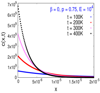
(a)

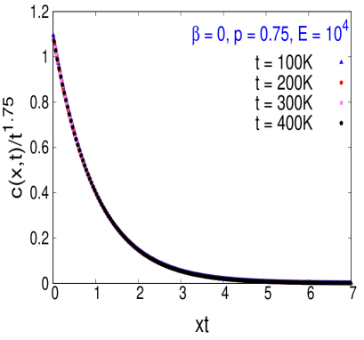
(b)

Figure 1: (a) The distribution function $c(t,x)$ is drawn as a function of $x$ for different time ($t=100,200,300,400$) with fixed $\beta=0$ and $p=0.75$ where $p$ is the probability with which the newly created fragment is kept in the system. (b) The same set of data set are used to plot them in the self-similar scale and find excellent data collapse. Here, all the plots represent ensemble average over $E=1\times 10^{4}$ independent realizations.

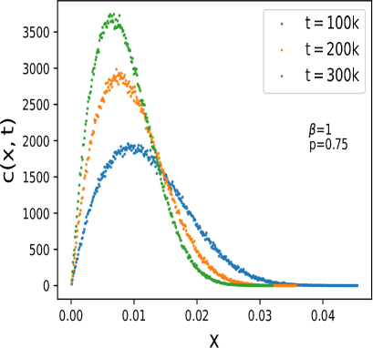
(a)

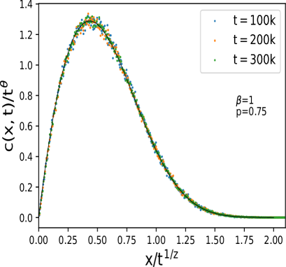
(b)

Figure 2: (a) The distribution function $c(t,x)$ is drawn as a function of $x$ for $\beta=1$. Each plot represents data obtained from snapshots taken at different time $t=100,200,300$. (b) The same set of data are used to plot them in the self-similar scale and find excellent data collapse revealing that $c(x,t)$ exhibits dynamic scaling.

I continued working on one dimensional fragmentation equation primarily the case where mass conservation is violated. We found that the violation of mass conservation is always accompanied by the emergence of stochastic fractal. On the hand, one of the essential criterion of fractal is self-similarity. In the case of stochastic fractal, self-similarity means that the distribution function $c(x,t)$ exhibits dynamic scaling

$$c(x,t)\sim t^{\theta z}\phi(x/t^{-z}),$$ (3)

where $\phi(\xi)$ is the scaling function, $\theta$ is the mass exponent and $z$ is the kinetic exponent ref.family_Vicsek ; ref.scaling . Note that the mass exponent $\theta=1+d_{f}$ where $d_{f}$ is the fractal dimension. It means that the plots of $c(x,t)$ versus $x$ plotted from the snapshots of the system taken at different time will be distinct. However, all these distinct plots collapse into a single universal scaling function if we plot $c(x,t)t^{-\theta z}$ versus $x/t^{-z}$ instead. In Figs. (1a) and (2a) we first plot distribution function $c(x,t)$ as a function of $x$ for dyadic Cantor set for $\beta=0$ and $\beta=1$ respectively to see how it varies with $\beta$ value ref.fractal_pandit ; ref.fractal_rakib . In Figs. (1b) and (2b) we use the same data to plot $c(x,t)t^{(1+d_{f})z}$ versus $x/t^{-z}$ and find excellent data collapse of all the distinct plots in Figs. (1a) and (2a) respectively. They suggest that the snapshots taken at different times are similar, which is also a kind of symmetry in continuous time. It has been shown that the fractal dimension $d_{f}$ increases with $\beta$ and for all $\beta$, the $d_{f}$th moment is always a conserved quantity ref.fractals_2002 . We have recently shown a connection between these conserved quantities and Noether’s theorem that states that where a continuous symmetry exists there must exist a conserved quantity ref.fractal_rakib .

Fragmentation equation never stopped giving surprising results. In 1996, we show that in planar fragmentation each non-trivial conserved quantity can be used as a multifractal measure ref.multifractality_pla ; ref.multifractality_pre . Besides this, the planar fragmentation can also be described as random sequential division of plane into mutually exclusive rectangular cells which we regarded as the weighted planar stochastic lattice (WPSL) ref.hassan_njp ; ref.hassan_jcp . One of the most interesting findings of this work is the emergence of infinitely many conserved quantities $\sum_{i}x_{i}^{m-1}y_{i}^{4/m-1}=1$ $\forall\ m$. Except $m=2$ case or the total mass conservation, all the other conserved quantities are highly non-trivial whose existence we only know because we can solve the problem analytically. A far more interesting fact is that each of the non-trivial conserved quantities can be regarded as the multifractal measure such the $i$ cell contains only $\mu_{i}(m)=x_{i}^{m-1}y_{i}^{4/m-1}$ of the total measure. The distribution of this measure can be best described as a multifractal. Since each of the infinitely many non-trivial conserved quantities can be a measure, there are thus infinitely many multifractal $f(\alpha)$ spectra where $\alpha$ is known as the Hölder exponent. Interestingly, if we replace the center of each cell of the WPSL by a node and common border between cells by a link between the corresponding node then it emerges as a scale-free network. More recently, we have solved a class of models where by dividing the plane vertically or horizontally with equal probability the resulting network is not only scale-free with smaller exponent of the power-law degree distribution but also small-world ref.tushar_hassan_1 ; ref.tushar_hassan_2 . It is small-world because we find that the mean geodesic path length increases logarithmically with system size and the total mean clustering coefficient is high and independent of system size. It implies that it is also a small-world network.

III Kinetics of aggregation

Yet another field of research where Ziff studied extensively and contributed enormously is the kinetics of aggregation or polymerization ref.ziff ; ref.ziffEtAl . The most successful equation that can describe the kinetic of aggregation process is the Smoluchowski equation

$${{\partial c(x,t)}\over{\partial t}}=-c(x,t)\int_{0}^{\infty}K(x,y)c(y,t)dy$$ (4)

$$+ {{1}\over{2}}\int_{0}^{x}K(y,x-y)c(y,t)c(x-y,t)dy,$$

where $K(x,y)$ is the aggregation kernel that describes the rate at which particle $x$ and $y$ meets ref.smoluchowski . The first (second) term on the right hand side of Eq. (5) describes the loss (gain) of size $x$ due to merging of size $x$ ($(x-y)$) with particle of size $y$.Unlike fragmentation equation, finding exact solution for various different choices of aggregation kernel $K(x,y)$ is still a formidable task. Robert Ziff focused mostly on long time limit or scaling solution. One of the most striking results is that the concentration $c(x,t)$ of particles of size $x$ at time $t$ exhibits dynamic scaling ref.gelation ; ref.scaling . Like shattering transition in fragmentation, Ziff has shown that for certain choice of aggregation kernel the Smoluchowski equation describes gelation transition ref.gelation ; ref.ziff_stell ; ref.ziff_ernst . It is a phase where the system loses its mass to gel phase. The sol-gel transition is a very interesting field of study due to its own right. His work led to extensive study of the Smoluchowski equation.

While I was working on my Phd on the kinetics of fragmentation, I was also reading articles on aggregation especially the articles authored by Ziff, Redner and Ernst. While reading articles and books, I realized that most numerical and experimental works suggest that almost always aggregates can be best described as fractal ref.vicsek ; ref.lin ; ref.weitz . However, despite extensive studies, there did not exist any analytically solvable model within the framework of Smoluchowski equation which can support this geometric aspect. Finding a model that can describe the emergence of fractal could help us know why the fractal is ubiquitous in the aggregation process. In 2008-2013, I was finally successful to find two different aggregation models within the framework of Smoluchowski equation which can account for the emergence of fractal ref.fractal_cda_1 ; ref.fractal_cda_2 ; ref.fractal_self . Interestingly, it has been found that fractal in fragmentation is only possible if the mass of the system is either removed or the size of the particles are continuously decreased, for instance by evaporation, while fractal in aggregation emerges only if mass is added or particles are continuously grown, say, by condensation. In general, for the emergence of fractal we must have a system which is open.

The first model was on aggregation of continuously growing particles by heterogeneous condensation which we solved exactly in one dimension ref.fractal_cda_1 . The generalized Smoluchowski (GS) equation that can describe condensation-driven aggregation is given by

$$\Big{[}{{\partial}\over{\partial t}} + {{\partial}\over{\partial x}}v(x,t)\Big{]}c(x,t)=-c(x,t)\int_{0}^{\infty}K(x,y)c(y,t)dy$$ (5)

$$+ {{1}\over{2}}\int_{0}^{x}dyK(y,x-y)c(y,t)c(x-y,t),$$

The second term on the left hand side of the above equation accounts for the growth by condensation with velocity $v(x,t)$. However, the GS equation can only describe the condensation-driven aggregation (CDA) model if the growth velocity $v(x,t)$, the collision time $\tau$, and the kernel $K(x,y)$ are suitably chosen. In the absence of the second term on the right hand side, Eq. (5) reduces to the classical Smoluchowski (CS) equation as given in (Eq. 4) whose dynamics is governed by the conservation of mass law ref.smoluchowski . To obtain a suitable expression for the elapsed time we do a simple dimensional analysis in Eq. (5) and immediately find that the inverse of $\int_{0}^{\infty}K(x,y)c(y,t)dy$ is the collision time $\tau(x)$ during which the growth $\alpha x$ takes place ref.maslov . The mean growth velocity between collisions therefore is

$$v(x,t)={{\alpha x}\over{\tau(x)}}=\alpha x\int_{0}^{\infty}dyK(x,y)c(y,t).$$ (6)

We choose a constant aggregation kernel to make the collision independent of the size of the colliding particle i.e.,

$$K(x,y)=2,$$ (7)

for convenience.

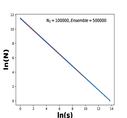
(a)

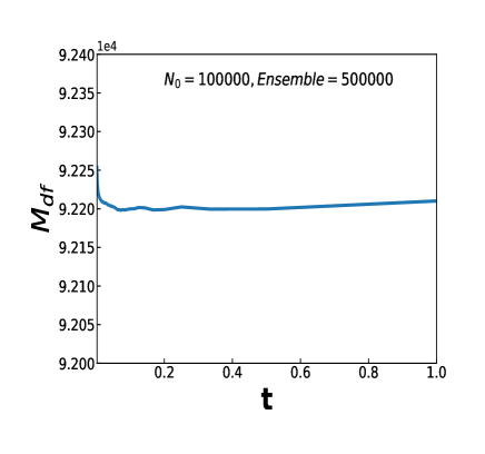
(b)

Figure 3: (a) We plot number $N$ versus mean particle size $s$ and find excellent straight line with slope $d_{f}=1/(1+2\alpha)$ that agrees perfectly with analyitcal solution. (b) The plot of the $d_{f}$th moment of $c(x,t)$ versus time $t$ shows it is indeed a conserved quantity. Here, $N_{0}$ is the initial number of mono-disperse particles and the data is averaged over $E=10^{4}$ number of independent realizations (ensemble size).

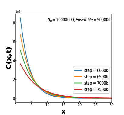
(a)

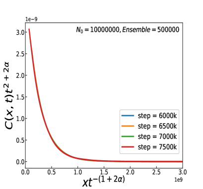
(b)

Figure 4: (a) The distribution function $c(t,x)$ is drawn as a function of $x$ for different times. The same set of data set of (a) are used to plot in them in the self-similar scale (b) and find excellent data collapse revealing $c(x,t)$ exhibits dynamic scaling.

We can solve Eq. (5) for constant kernel with condensation velocity given by Eq. (6) analytically and solve it numerically using the following algorithm.

• The process starts with $N$ number of particles of equal sized particles (however we can choose any distribution since the results are independent initial condition).

• Two particles are picked randomly from the system to mimic random collision via Brownian motion.

• The sizes of the two particles are increased by a fraction $\alpha$ of their respective sizes in the logbook to mimic the growth by condensation.

• Their sizes are combined to form one particle to mimic the aggregation process.

• The logbook is updated by registering the size of the new particle in it and at the same time deleting the sizes of its constituents from it.

• The steps (ii)-(v) are repeated ad infinitum to mimic the time evolution.

Extensive Monte Carlo simulation gives that mean particle size $s(t)$ grows following a power-law

$$s(t)\sim t^{(1+2\alpha)}.$$ (8)

If the size of the total size of the aggregates are measured using mean particle size as an yard-stick we find that this number decays with $s$ following a power-law

$$N(s)\sim s^{-d_{f}},$$ (9)

where $d_{f}$ is the fractal dimension given by

$$d_{f}={{1}\over{1+2\alpha}},$$ (10)

as shown in Fig. (3a). We also find that $d_{f}$th moment of $c(x,t)$ is a conserved quantity and our numerical simulation also confirm this in Fig. (3b). Note also that the distribution function $c(x,t)$ obeys dynamic scaling

$$c(x,t)\sim t^{-(1+d_{f})z}\phi(x/t^{z}),$$ (11)

where $z=1+2\alpha$ and $\phi(x)$ is the scaling function ref.hassan_ba_dc . It implies that the distinct plots as shown in Fig. (4a) of $c(x,t)$ versus $x$ at different time should collapse into universal curve. To prove this we then plot $c(x,t)t^{(1+d_{f})z}$ versus $x/t^{z}$ in Fig. (4b) and find an excellent data collapse.

The second model was on the kinetics of aggregation of Brownian particles with stochastic self-replication ref.fractal_self . It is a very simple variant of the Smoluchowski equation in which we investigate aggregation of particles accompanied by self-replication of the newly formed particles with a given probability $p$. That is, we may consider that the system has two different kinds of particles: active and passive. As the systems evolves, active particles always remain active and take part in aggregation while the character of the passive particles are altered irreversibly to an active particle with probability $p$. Once a passive particle turns into an active particle it can take part in further aggregation like other active particles already present in the system on an equal footing and never turns into a passive particle. The definition of the model in some sense is reminiscent of the dyadic Cantor set as we just have to replace the co-factor ${{1}\over{2}}$ of the gain term of Eq. (4) by ${{1+p}\over{2}}$.

Like the previous model, the results of this model can be generalized if we express everything in terms of $d_{f}$ and $z$. The only way, the two results differs are in the value of $d_{f}$ and $z$ as we find that $d_{f}=(1-p)/(1+p)$ and $z=(1+p)/(1-p)$. The results from the two opposing phenomena reveal that fractal emerges only if the total mass of the system grows with time following a power-law in aggregation and in fragmentation process fractal emerges only if the total mass decreases with time. The opposite reasons for the emergence of fractal reflects the inherent opposing nature of the two phenomena. In all these kinetic systems, the emergence of fractal is always accompanied by the conservation of the $d_{f}$th moment of $c(x,t)$ ref.fractal_conserved .

IV Kinetics of random sequential adsorption process

Random sequential adsorption (RSA) is yet another field of research where Robert Ziff worked quite extensively ref.rsa_ziff_1 ; ref.rsa_ziff_2 ; ref.rsa_ziff_3 . One of the results that I really liked in RSA is the jamming limit for RSA of monodisperse particle, which is also known as car-parking problem, in one dimension as it can be solved exactly ref.car_parking . It has been found that the fraction of the total space being occupied by the depositing particles is $0.7475979203..$, provided sizes of the depositing particles are negligibly smaller than the size of the substrate ref.renyi . However, most of his work has been on two dimensional substrate which is physically more relevant than its one dimensional case. In two dimensions, works are mostly done by numerical simulation. I was interested more on analytical solution and hence concentrated only on one dimension. I solved RSA model for a mixture of two different sized particles, a mixture of particles that follows a power-law and a mixture of point like and fixed sized particles ref.hassan ; ref.hassan_rsa1 ; ref.hassan_rsa2 .

V Thermodynamic formalism of percolation

The field of research where Robert Ziff has contributed the most is the theory of percolation ref.per_ziff_1 ; ref.per_ziff_2 ; ref.per_ziff_3 ; ref.per_ziff_4 . Percolation model is perhaps one of the most elegant concept in statistical physics which can be used in many different situations of science, arts and social science. Despite being first conceived in 1941 by Flory, its mathematical formulation was first given in 1957 by Broadbent and Hammersley ref.Broadbent . Since then it has been one of the most studied models. As far as the definition of percolation model is concerned everyone would agree that it is one of the simplest models in statistical physics ref.Stauffer . On the other hand, it is also one of the hardest models in statistical physics since we only have a few exact solution in dimensions $1<d<\infty$. The idea of percolation was first conceived in the early 1940’s by chemist Paul Flory in his study on gelation in polymers, although he did not use the word ”percolation” ref.Flory . The very word ”percolation” was first used and its mathematical formulation was first proposed by engineer Simon Broadbent and mathematician John Hammersley in 1957 ref.Broadbent . In their seminal paper, the authors clearly stated that their work has the potential to encourage others to investigate this terrain, which has both pure mathematical fascinations and many practical applications. Indeed, the following years, namely the entire 60s decade, the works of a group of celebrity researchers like Cyril Domb, Michael Fisher, John Essam, and M.F. Skyes, Rushbrooke, Stanley, Coniglio, Halperin, Herrmann, Stauffer, Aharony, Havlin, Duplantier, Cardy, Grassberger and Ziff popularized the percolation problem among both physics and mathematics communities by establishing percolation as a critical phenomena ref.domb_1 ; ref.domb_2 ; ref.domb_3 ; ref.essam_1 ; ref.essam_2 .

The simplest way to define percolation is to first choose a lattice or network as a skeleton and assume that initially all the disconnected sites are present so that each site is a cluster of its own size. As we occupy bonds, we find that for small occupation probability $p$ there are only small isolated clusters that do not span across the entire lattice and if $p$ is close to one there will definitely a cluster which would span the lattice. Thus, there exists a critical or threshold value so that in the thermodynamic limit at $p>p_{c}$ the system will at least have one cluster that spans across the linear size of the lattice ref.Stauffer ; ref.saberi . Finding percolation thresholds $p_{c}$ both exactly and by numerical simulation has been an enduring subject of research in percolation. Robert Ziff found critical points for many different lattices and made significant contributions to exact solutions both on the lattice level, in the continuum limit and on the networks too ref.per_ziff_1 ; ref.per_critical_1 ; ref.per_critical_2 . Besides, finding an efficient algorithm for percolation is always considered significant development as that would mean we can simulate for larger system size and get results for higher ensemble size. To this end, the first and most classic algorithm is the Hoshen and Kopelman algoritthm and later the Leath algortithm ref.hoshen ; ref.leath . However, the last and currently most efficient algorithm is the Newman and Ziff algorithm ref.per_ziff_0 ; ref.per_ziff_algorithm . It measures an observable quantity in a percolation system for the full spectrum of occupation probability $p$ in an amount of time that scales linearly with the system size. In that article, Newman and Ziff also showed how to get an observable as function of $p$ from the data as a function of the number of occupied bonds $n$ which gives the results in the canonical ensemble. The data obtained in the canonical ensemble makes the ensemble average computationally much cheaper and smoother.

One of the major breakthrough was made by Kasteleyn and Fortuin in 1969 who showed that q-state Potts model in the limit $q\rightarrow 1$ corresponds to percolation model ref.Kasteleyn . It paved the way to identify the equivalent counterpart of order parameter and susceptibility in percolation which was crucial to prove that percolation is indeed a model for second order phase transition and to find the corresponding critical exponents. The best known example of the second order phase transition is the paramagneitc to ferromagnetic transition or vice versa and the simplest model that can capture its various aspects successfully is the Ising model. Despite its simplicity, its exact solution in two or in higher dimensions remained an open problem for many years until Onsager solved it exactly. However, a more physical understanding of the phenomena was made by Wilson, Fisher and Kadanoff who showed that the system at and near the critical point is scale invariant ref.kadanoff ; ref.wilson ; ref.fisher . It means that if we blow up the picture near the critical point by some factor $b>1$ then it would look the same, at least in the statistical sense. This simple idea played a crucial role for the renormalisation group which led to a deeper understanding of the critical phenomena including percolation. Soon, Alexander Polyakov established a connection between the idea of scale invariance and the conformal invariance ref.polyakov . Polyakov argued that the picture of the system should also remain statistically similar if the factor $b$ is allowed to vary smoothly as a function of the called conformal mappings. Stanislav Smirnov was awarded Fields Medal in 2010 for his proof of conformal invariance at criticality ref.smirnov .

I was so much inspired by the work of Robert Ziff on percolation that I always wanted to do something with it. Teaching is the best way to learn a subject. To that end, in 2005 I designed a course titled ”Non-equilibrium Statistical Mechanics” and included percolation in the chapter of phase transition and critical phenomena. That was the time I really began to understand the subject. That is the time when I also realized that despite the 60-year-long active research on percolation we still did not know how to define entropy. This is one of the most crucial quantity for defining the order of transition since without it, we can never know specific heat and whether the transition involves any latent heat or not. Besides, I also realized that the critical exponents of percolation must also obey the Rushbrooke inequality. In other words, for every quantity that we have in thermal phase transition we must have an exact equivalent counterpart in percolation.

The first question I wanted to explore is: What if I replace a regular planar lattice with a weighted planar stochastic lattice (WPSL) as a skeleton. We proposed this lattice in 2010 and shown that it is multifractal and, unlike square or regular lattice, its coordination number is not fixed rather exhibits a power-law. I engaged one of my MS thesis students to work on this problem in 2014 and in 2015 we had our first article published in the Physical Review E as a rapid communication ref.hassan_mijan_1 ; ref.hassan_mijan_2 . One of the interesting findings of phase transition and critical phenomena in general is the universality class. It is one of the central predictions of renormalisation group theory that the critical behaviours of many statistical mechanics models on Euclidean lattices depend only on the dimension and not on the specific choice of lattice. As far as regular Euclidean lattice is concerned, it has been found that the critical exponents of percolation too depends only on the dimension of the lattice and are independent of the details of the lattice. Our work on WPSL suggests that it is, however, not true if the planar lattice is scale-free and multifractal. This is perhaps the only known exception where despite its dimension is the same as that of the square or triangular lattice yet it belong to different universality class.

Percolation is well known as a model for second order phase transition since the later part of the 60s decade. Second order phase transitions occur when a new state of reduced symmetry develops continuously from the higher symmetric disordered (high temperature) phase. In fact, two quantities are crucial to determine the order of transition: order parameter and entropy. Order parameter quantifies the extent of order and entropy measures the degree of disorder. A full descriptions of phase transition is only possible if we know the behavior of both the quantities. However, in the last 60 years enough attention has not been paid to know how to measure entropy for percolation. To the best of our knowledge, the first attempt to obtain entropy in percolation was made by Tsang and Tsang in 1999 and a slightly different definition was used by Vieira et. al in 2015 ref.tsang ; ref.tsang_1 ; ref.Vieira . They both found that entropy is maximum at the critical point and zero at the initial state. We all know that order parameter too is zero at the initial state and remain zero till the critical point. However, due to finite-size effect order parameter can be non-zero but small near the critical point. However, the behavior of order parameter for increasingly larger system size clearly shows the sign of becoming zero in the thermodynamic limit up to the critical point. If initially entropy and order parameter are both equal to zero it means that the system is at the same time in a perfectly ordered and disordered state. This cannot be right and hence something must be wrong in their choice of probability to define entropy. That was the time when I started my journey to find a proper way of obtaining entropy for percolation.

In 2017, we were successful as we used cluster picking probability $\mu_{i}=s_{i}/N$ where $s_{i}$ is the size of the $i$th cluster and $N$ is the system size ref.hassan_didar ; ref.hassan_shahnoor . It describes the probability that a site, picked at random, belongs to the $i$th cluster. Using this probability in the definition of Shannon entropy

$$H=-K\sum_{i}\mu_{i}\log\mu_{i},$$ (12)

where the constant $K$ just amounts to a choice of a unit of measure of entropy and hence we choose $K=1$ for convenience ref.shannon . It gives the desired entropy which is consistent with the nature of order parameter. Substituting $\mu_{i}=s_{i}/N$ in Eq. (12) we get

$$H = -{{1}\over{N}}\sum_{i}s_{i}\log s_{i}+{{1}\over{N}}\sum s_{i}\log N$$

$$= {{1}\over{N}}\log{{N!}\over{s_{1}!s_{2}!....s_{k}!}}={{1}\over{N}}\log\Omega,$$

where $\Omega$ is the number of distinct ways $N$ number of sites can be arranged into $k$ number of clusters of sizes $s_{1},s_{2},...,s_{k}$. Thus, the Boltzmann entropy for that specific state is $S=k_{B}\ln\Omega$. If we choose the Boltzmann constant $k_{B}=1$, for convenience, since it merely amounts to the choice of the measure of entropy then we find that Shannon entropy actually is the entropy per site In other words, the Shannon entropy is the specific entropy and the total entropy $S$ is equal to $S=NH$ which makes it an extensive property as it should be.

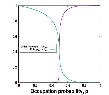
(a)

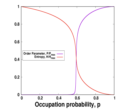
(b)

Figure 5: Plots of scaled order parameter $P(p)/P(1)$ and scaled entropy $H(p)/H(0)$ as a function of occupation probability $p$, fraction of bond (site) being occupied, for lattice size of linear size $L$ are shown in the same plot for (a) bond (b) for site percolation. In (a) both cases the two curves meet almost at the critical occupation probability $p_{c}$.

We start the percolation process such that initially every site is isolated and hence there are $N=L^{2}$ number of equal sized cluster of size one in the square lattice of linear size $L$. Initially, $\mu_{i}=1/N\ \forall\ i$ and hence substituting it in Eq. (12) yields $H(0)=\log(N)$ which is the maximum possible entropy. This situation is analogous to ideal gas which corresponds to the most disordered state since the entropy is maximum. In percolation, the maximum entropy at $p=0$ is consistent with the behavior of order parameter $P$ since we have $P=0$ at $p\leq p_{c}$. At other extreme when all the sites are connected we have $\mu_{i}=1$ and thus entropy is equal to zero. This state can be regarded as analogous to crystal state where there is just one perfectly ordered microstate. This state of $H=0$ is again consistent with the behavior of order parameter as we find that the order parameter $P$ is maximally high. Thus, it suggests that the system is almost in the perfectly ordered state. The second order or continuous phase transition is also known to be accompanied by an order-disorder transition although in percolation this aspects of phase transition have never been looked at. Plotting entropy and order parameter in the same graph can provide better insights into this. To this end, we plot both $H$ and $P$, though we re-scaled both entropy and order parameter by $H(0)$ and $P(1)$ respectively, in the same graph for random bond and site percolation as shown in Figs. (5a) on square lattice. We see a sharp and sudden change of both quantities near $p_{c}$ and they both meet almost at $p_{c}$. This is a sign of order disorder transition as we see that at $p<p_{c}$ order parameter $P$ is minimally low where entropy is maximally high and vice versa at $p>p_{c}$. Thus, the $H-P$ plot suggests that the transition is accompanied by an order-disorder transition ref.hassan_didar ; ref.hassan_shahnoor .

While measuring entropy for site percolation on square lattice we have found that it suffers a problem. In the traditional definition of site percolation we occupy a site and we measure the cluster size in terms of the number of contiguous occupied sites. On the other hand, in bond percolation we occupy a site and measure cluster in terms of the number of contiguous sites connected by the occupied bonds. That is, there are two entities, namely bonds and sites, such that when bonds are occupied we must connect sites and vice versa. This has not been the case for the traditional definition of site percolation. We therefore recently redefined site percolation ref.hassan_shahnoor . We assume that initially all the isolated bonds are already present in the system. The occupation of sites then connects the bonds and cluster sizes are measured by the number of contiguous bonds connected by the occupied sites. Interestingly, the new definition of site percolation does not change the values of the critical point and the critical exponents except now the behavior of entropy is consistent with the order parameter. We now show the plots of order parameter and entropy in Fig. (5b) according to the new definition of site percolation. The plots of $H$ and $P$ meet near the critical point like for bond percolation suggesting that site percolation too is accompanied by order-disorder transition.

One of the reasons why percolation is so elegant and has been well studied for more than 60 years is that it has many features in common with its thermal counterpart. One of the features is definitely the universality. We know that the critical exponents in thermal phase transition depend only on the dimension of the lattice or system, the spin dimensions and the extent up to which spin can interact. Interestingly, their values are independent of the detailed nature of the lattice structure and the strength of interaction. The critical exponents in percolation too are well-known to depend only on the dimensions of the lattice or system and independent of the types of percolation, namely whether the percolation is bond and site type, as well as of the detailed structure of the lattice. However, in 2015 we find that this is no longer the case if the lattice is multifractal and scale-free as we find that its coordination number distribution obeys inverse power-law. That is, we performed percolation on WPSL which is a planar lattice and hence it was expected to belong to the same university class as that of square lattice ref.hassan_mijan_1 . Instead, we, find new set of critical exponents that clearly suggests that scale-free and multifractal nature have an impact in determining the universality class.

Besides Euclidean regular and scale-free lattice as a skeleton for percolation, the use of network (random, scale-free and small-world networks) as a skeleton is gaining increasingly more popularity. Networks are not embedded in the Euclidean space rather in the abstract space. Networks can mimic many real-life systems such as transportation network (like the world-wide airline network) or a communication network (like world wide web network). Besides, viruses are typically spread on a social or through computer network and hence whether such spreading will cause epidemic or pandemic or will just die out will depend on the nature of its network architecture. The history of percolation on random graph goes back to the work of Erdös and Rényi in 1959 ref.erdos . The process starts with $N$ isolated nodes and we connect them by adding links one at each step after picking them randomly. It is intuitively clear that as the number of added links $n$ is increased, contiguous occupied nodes keep forming clusters and their average size continue to grow. Even in such simple process we observe that suddenly a giant cluster, whose size is $O(N)$, emerges across a critical point $t=1/2$ where the relative link density $t=n/N$. Note that in the stochastic processes like fragmentation and aggregation $t$ is regarded as time. It is also important to note that in the context of percolation on network $t$ plays the same role as occupation probability $p$ of percolation on lattice. Erdös and Rényi demonstrated that below $t_{c}$ even the largest cluster $s_{{\rm max}}$ is of miniscule size $O(\log N)$ ref.erdos ; ref.bollobas . The transition from such miniscule to a giant cluster is called percolation which is analogous to the transition from non-spanning to spanning cluster in a spatially embedded lattice.

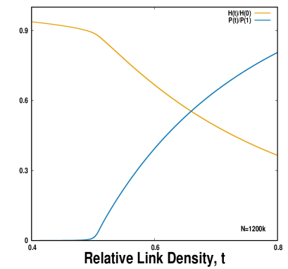
(a)

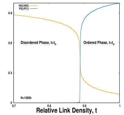
(b)

Figure 6: Plots of scaled order parameter $P(t)/P(1)$ and scaled entropy $H(t)/H(0)$ as a function of $t$ for fixed network size $N$ are shown in the same plot for (a) ER (b) for EP.

It is true that percolation in random or Erdös and Rényi graph describes a phase transition. However, the order transition and the nature of symmetry breaking have never been clearly stated. Our plots of entropy and order parameter for percolation on ER network suggests that above $t_{c}$ they both are sufficiently high as seen in Fig. (6a). It means above $t_{c}$ the system is moderately ordered and moderately disordered at the same time. It also means that ER transition is clearly not an order disorder transition. The situation changes, however, if we pick two links randomly instead of one at each step but occupy only the one that forms a smaller cluster than the other link, which we then discard. As the growth of the larger cluster is systematically discouraged, the transition is delayed which is expected but when it happens it undergoes a transition in an explosive fashion and hence it was termed as an ”explosive percolation” by Achlioptas et. al in 2009 ref.Achlioptas . Initially, it was mistaken as discontinuous or first order transition but finally in 2011 it was shown to describe second order transition. This time the order parameter $P$ and entropy $H$ undergo a much sharper transition than the ER transition. It can be easily seen in Fig. (6b)that where $P$ is minimally low and $H$ is maximally high and vice versa suggesting it is truly an order-disorder transition.

The question is: Why do we get sharp order-disorder transition when we encourage smaller cluster to grow faster than the larger cluster? Friedman and Landsberg argued that encouraging the smaller cluster to grow faster helps the system develops powder keg and eventually the mitigation of this effect results in the explosive percolation which is called powder keg ref.Friedman . However, the exact physics behind this powder keg effect has not been explained yet. We know the expression for free energy $F=E-TS$ from thermodynamics. In a given situation the minimum of $F$ always corresponds to the stable state. Due to the competing role of $E$ and $S$, the minimum of $F$ can be achieved in two ways: In the disordered phase, the minimum of $F$ is achieved by maximizing $S$ and in the low temperature phase the minimum of $F$ is achieved by minimizing $E$. In percolation, initially at $t=0$ the system is at its maximum entropy or at its utmost disordered phase. Thus, when there are options available the system will choose the one that minimizes $F$. In explosive percolation, adding the link that forms smaller cluster helps the system continue to stay at a higher entropy state. Note that increasing the number of available options makes the system stays longer at a higher entropy state and hence the onset of transition is delayed further thus making the transition at a higher $t_{c}$ value. However, regardless of the number of options we choose, the critical point $t_{c}$ never exceeds one. It suggests that we can consider $1-t$ as the equivalent counterpart of temperature.

VI Discussion and conclusions

In this article, I have tried to outline the research field of Robert Ziff alongside my contribution to the fields as motivated by his works. I started with the kinetics of fragmentation where Ziff obtained many exact solutions to the fragmentation equation. The most significant finding of him in fragmentation is the shattering transition where the smaller particles breaks at an increasingly rapid rate that results in the loss of mass to the ”zero size” phase. This is in some sense reminiscence of Bose-Einstein condensation. I then discussed how we can use the fragmentation equation in one dimension to describe fractal and in higher dimensions multifractal. A system that evolves in time in such a way that all snapshots are similar in the same sense as two or more triangles are similar is said to obey dynamic scaling. Self-similarity in continuous time axis is also a kind of continuous symmetry. It suggests that there must be a conserved quantity as a controlling agent behind preserving this self-similarity along the time axis. When the total mass is a conserved quantity the system is not a fractal. When the mass of the system is not a conserved quantity the system is a fractal provided there still exists a conserved quantity required by the self-similar symmetry which is reminiscence of Noether’s theorem. The conserved quantity in the $d_{f}$th moment of the fragments size distribution function $c(x,t)$.

I then discussed about the opposite of fragmentation phenomena namely the kinetics of aggregation in which Ziff has made significant contribution too. Apart from finding the scaling solution to the Smoluchowski equation, the most significant finding is that under certain conditions it can describe gelation transition which is just opposite to shattering transition. I have shown that the Smoluchowski equation can describe fractal too but only if the total mass of the system grows with time following a power-law. The resulting system also exhibits dynamic scaling - a litmus test of continuous self-similarity along time axis. Like the emergence of fractal in fragmentation, here too we find that the $d_{f}$th moment of $c(x,t)$ is a conserved quantity which essentially controls the self-similar symmetry along time axis. Thus, the emergence of fractal in both aggregation and fragmentation shares some common features. Namely, (i) they both exhibit dynamic scaling, (ii) total mass in fragmentation must decrease and increase in aggregation but in both the cases they do it following a power-law.

Finally, I discuss the various new aspects of percolation theory where Robert Ziff’s contribution is truly outstanding. Percolation is the simplest model in statistical physics that describes second order phase transition. Real thermal physical system that exhibits second order phase transition is also accompanied by order-disorder transition. It also means symmetry is broken as the system undergo transition from disordered to order which forms the heart of Landau theory of phase transition. For more than 60 years we only knew how to measure the extent of order as we could measure order parameter for percolation. To know whether the transition also breaks symmetry or not we must know how to measure entropy for percolation. Recently, I have defined entropy for percolation which paved the way to define specific heat too. Furthermore, I have recently redefined susceptibility since the critical exponent $\gamma$ obtained from mean cluster size was too high to obey Rushbrooke inequality with positive value of $\alpha$ of the specific heat. The critical exponents obtained from the redefined quantities obey the Rushbrooke inequality for random and explosive percolation on network and lattice both. Besides, I have discussed about the role of entropy in checking whether percolation is also accompanied by order-disorder transition. To that end, it has been found that percolation on ER network does not break symmetry or is not accompanied by order-disorder transition unlike explosive percolation.

We all know that gravitational forces not only act on things that are close together but they also act on things that are at great distances apart. The Earth and Moon are 384,400 km apart and yet gravity creates an immense force which is often referred to as action at a distance. Like wise researchers can create a generation of new researchers through their published works which can also be referred as action at a distance. We do PhD under a direct supervisor but we often fail to recognise that we are also being supervised by many action at a distance supervisors. Through this Robert Ziff and many others like him have been influencing new generation of researchers. In this article I tried to emphasize this. In conclusion, I have given a comprehensive account of fragmentation, aggregation and percolation processes and tried to outline their key features. I dedicate this paper to Robert Ziff on the occasion of his 70th birthday whose scientific leadership and influential works have been continuously guiding, inspiring, and challenging my generation and will continue to do so to the generation to come.

References

- (1) R. M Ziff and E. D. McGrady, J. Phys. A: Math. Gen. 19 3027 (1985)
- (2) R. M. Ziff, J. Phys. A: Math. Gen. 24 2821 (1991).
- (3) R. M Ziff and E. D. McGrady, Macromolecules 19 2513 (1986).
- (4) G. J. Rodgers and M. K. Hassan, Phys. Rev. E 50 3458 (1994).
- (5) M. K. Hassan, Phys. Rev. E 55 5302 (1997).
- (6) M. K. Hassan, J. Kurths, J. Phys. A: Math. Gen. 34 7517 (2001).
- (7) M. K. Hassan, J. Schmidt, B. Blasius, J. Kurths, Phys. Rev. E 65 045103 (2002).
- (8) M. K. Hassan and M. Z. Hassan, Phys. Rev. E 77 061404 (2008).
- (9) M. K. Hassan and M. Z. Hassan, Phys. Rev. E 79 021406 (2009).
- (10) M. K. Hassan, M. Z. Hassan and N. Islam, Phys. Rev. E 88 042137 (2013).
- (11) M. E. J. Newman, R. M. Ziff, Phys. Rev. Lett. 85 4104 (2000).
- (12) M. E. J. Newman, R. M. Ziff, Phys. Rev. E 64 016706 (2001).
- (13) R. M. Ziff, Phys. Rev. Lett. E 69 2670 (1992).
- (14) J. Quintanilla, S. Torquato, R. M. Ziff, J. Phys. A: Math. Gen. 33 L399 (2000).
- (15) P. N. Suding, R. M. Ziff, Phys. Rev. E 60 275 (1999).
- (16) C. R. Scullard, Robert M Ziff, Phys. Rev. E 73 045102 (2006).
- (17) M. E. J. Newman, R. M. Ziff, Phys. Rev. E 66 016129 (2002).
- (18) I. R. Tsang and I. J. Tsang, Phys. Rev. E 60 2684 (1999).
- (19) I. J. Tsang, I. R. Tsang, and D. Van Dyck, Phys. Rev. E 62 6004 (2000).
- (20) T. M. Vieira, G. M. Viswanathan, and L. R. da Silva, Eur. Phys. J. B 88 213 (2015).
- (21) D. Achlioptas, R. M. D’Souza, and J. Spencer, Science 323 1453 (2009).
- (22) Raissa M. D’Souza and J. Nagler, Nature 11 531 (2015).
- (23) P. Erdös, A. Rényi, Publ. Math. Inst. Hungar. Acad. Sci. 5 17 (1960).
- (24) E. J. Friedman and A. S. Landsberg, Phys. Rev. Lett. 103 255701 (2010).
- (25) R. M. Ziff, Phys. Rev. Lett. 103 045701 (2009).
- (26) F. Radicchi and S. Fortunato, Phys. Rev. Lett. 103 168701 (2009).
- (27) R. A. da Costa, S. N. Dorogovtsev, A. V. Goltsev, J. F. F. Mendes, Phys. Rev. E 91 042130 (2015).
- (28) R. M. D’Souza and M. Mitzenmacher, Phys. Rev. Lett. 104 195702 (2010).
- (29) Y. S. Cho, J. S. Kim, J. Park, B. Kahng, and D. Kim, Phys. Rev. Lett. 103 135702 (2009).
- (30) N. A. M. Araújo and H. J. Herrmann, Phys. Rev. Lett. 105 035701 (2010).
- (31) J. Nagler, A. Levina, and M. Timme, Nature Physics, 7 265 (2015).
- (32) R. A. da Costa, S. N. Dorogovtsev, A. V. Goltsev and J. F. F. Mendes, Phys. Rev. Lett. 105 255701 (2010).
- (33) P. Grassberger, C. Christensen, G. Bizhani, S-W Son, and M. Paczuski Phys. Rev. Lett. 106 225701 (2011).
- (34) O. Riordan and L. Warnke, Science 333 322 (2011).
- (35) L. Tian and D-N. Shi, Phys. Lett. A 376 286 (2012).
- (36) R. M. Ziff, E. Gulari, Y. Barshad, Phys. Rev. Lett. 56 2553 (1986).
- (37) R. M. Ziff, E. D. McGrady, Phys. Rev. Lett. 58 892 (1987).
- (38) Kinetics of Aggregation and Gelation, edited by F. Family and D. P. Landau (Elsevier, Amsterdam, 1984).
- (39) R. Shinnar, J. Fluid. Mech. 10 259 (1961).
- (40) R. Meyer, K. E. Alminand B. Steenberg, Brit. J. Appl. 11 Phys. 17 409 (1966).
- (41) W. R. Jhonson and C. C. Price, J. Polym. Sci. 45 217 (1960).
- (42) E. W. Merrill, H. S. Mickley and A. J. Ram, J. Polym. Sci. 62 S109 (1962).
- (43) P. L. Krapivsky and E. Ben-Naim, Phys. Rev. E 50 3502 (1994)
- (44) D. Boyer, G. Tarjus and P. Viot, Phys. Rev. E 51 1043 (1995).
- (45) P. L. Krapivsky and E. Ben-Naim, Phys. Lett. A 196 168 (1994).
- (46) M. K. Hassan and G. J. Rodgers, Phys. Lett. A 208 95 (1995).
- (47) M. K. Hassan and J. Kurths, Physica A, 315 342 (2002).
- (48) F. Family and T. Vicsek, J. Phys. A: Math. Gen. 18 L75 (1985).
- (49) Z. Cheng and S. Redner, Phys. Rev. Lett. 60 2450 (1988).
- (50) M. K. Hassan, N. I. Pavel, R. K. Pandit and J. Kurths, Chaos Soliton. Fract. 60 31 (2014)
- (51) R. Rahman, F. Nowrin, M. S. Rahman, J. A. Wattis, M. K. Hassan, Phys. Rev. E 103 022106 (2021).
- (52) M. K. Hassan, G. J. Rodgers, Phys. Lett. A 218 207 (1996).
- (53) M. K. Hassan Phys. Rev. E 54 1126 (1996).
- (54) M. K. Hassan, M. Z. Hassan and N. I. Pavel, New J. Physics, 12 093045 (2010).
- (55) M. K. Hassan, M. Z. Hassan and N. I. Pavel, J. Phyis. Conf. Ser. 297 012010 (2011).
- (56) T. Mitra and M. K. Hassan, Chaos Soliton. Fract. 154 111656 (2022).
- (57) T. Mitra and M. K. Hassan, Eur. Phys. J. Spec. Top. 230 3835 ((2021).
- (58) R. M. Ziff, J. Stat. Phys. 23 241 (1980)
- (59) R. M. Ziff, E. M. Hendriks and M. H. Ernst, Phys. Rev. Lett. 49 593 (1982).
- (60) M. von Smoluchowski, Z. Phys. Chem., Stoechiom. 92, 215 (1917).
- (61) R. M Ziff, G Stell, J. Chem. Phys. 73 3492 (1980).
- (62) R. M Ziff, M. H. Ernst, E. M. Hendriks, J. Phys. A: Math. Gen. 16 2293 (1983).
- (63) T. Vicsek, Fractal Growth Phenomena, 2nd ed. (World Scientific, Singapore, 1992).
- (64) M. Y. Lin, H. M. Lindsay, D. A. Weitz, R. C. Ball, R. Klein, and P. Meakin, Nature 339 360 (1989).
- (65) D. A. Weitz, J. S. Huang, M.Y. Lin, and J. Sung, Phys. Rev. Lett. 53 1657 (1984); ibid, 54 1416 (1985).
- (66) D. L. Maslov, Phys. Rev. Lett. 71 1268 (1993).
- (67) M. K. Hassan, M Z. Hassan and N. I Pavel, J. Phys. A: Math. Gen. 44 175101 (2011).
- (68) MK Hassan, Eur. Phys. J Spec. Top. 228 209 (2019)
- (69) R. D. Vigil, R. M. Ziff, J. Chem. Phys. 91 2599 (1989).
- (70) R. D. Vigil, R. M. Ziff, J. Phys. A: Math. Gen. 23 5103 (1990).
- (71) P. Kubala, M. Cieśla, R. M. Ziff, Phys. Rev. E 100 052903 (2019).
- (72) P. L. Krapivsky, J. Stat. Phys. 69 135 (1992).
- (73) A. Rényi, Transl. Math. Stat. Probab. 4 203 (1963).
- (74) P. N. Suding, R. M. Ziff, Phys. Rev. E 60 275 (1999).
- (75) R. M. Ziff, Phys. Rev. Lett. 56 545 (1986).
- (76) S Boettcher, J. L. Cook, R. M. Ziff, Phys. Rev. E 80 041115 (2009).
- (77) R. M. Ziff, C. D. Lorenz, P Kleban, Physica A 266 17 (1999).
- (78) S.R. Broadbent, J.M. Hammersley, Proc. Cambridge Philos. Soc. 53, 629 (1957).
- (79) D. Stauffer and A. Aharony, Introduction to Percolation Theory (Taylor Francis, London, 1994).
- (80) P.J. Flory, J. Am. Chem. Soc. 63 3083 (1941).
- (81) C. Domb and C. J. Pearce, J. Phys. A: Math Gen. 9 L137 (1976)
- (82) C. Domb and E. Stoll, J. Phys. A: Math. Gen. 10 1141 (1977)
- (83) C. Domb and M. F. Sykes Proc. R. Soc. A 240 214 (1957).
- (84) J.W. Essam, Rep. Prog. Phys. 43 833 (1980).
- (85) M.E. Fisher, J.W. Essam, J. Math. Phys. 2 609 (1961).
- (86) A. A. Saberi, Phys. Rep. 578 1 (2015).
- (87) R. M. Ziff, Phys. Rev. Lett. 69 2670 (1992).
- (88) K.J. Schrenk, N.A.M. Araújo, H.J. Herrmann, Phys. Rev. E 87 032123 (2013).
- (89) J. Hoshen, R. Kopelman, Phys. Rev. B 14 3438 (1976).
- (90) P.L. Leath, Phys. Rev. B 14 5046 (1976).
- (91) P. W. Kasteleyn and C. M. Fortuin, J. Phys. Soc. Japan 26 (Suppl.) ll (1969).
- (92) L. P. Kadanoff, Physics Physique Fizika. 2 263 ((1966).
- (93) K. G. Wilson, Phys. Rev. B. 4 (9) 3184 (1971).
- (94) M. E. Fisher, Rev. Mod. Phys. 46 597 (1974).
- (95) A. M. Polyakov, Sov. Phys. JETP Lett. 12 381 (1970).
- (96) S. Smirnov, C. R. Acad. Sci. Paris I 333 239 (2001).
- (97) M. K. Hassan and M. M. Rahman, Phys. Rev. E 92 040101(R) (2015)
- (98) M. K. Hassan and M. M. Rahman, Phys. Rev. E 94 042109 (2016).
- (99) M. K. Hassan, D. Alam, Z. I. Jitu and M. M. Rahman, Phys. Rev. E, 96 050101(R) (2017).
- (100) M. S. Rahman and M. K. Hassan, Phys. Rev. E 100 062109 (2019).
- (101) C. E. Shannon, Bell System Technical Journal 27 379 (1948).
- (102) B. Bollobás, Trans Amer Math Soc 286 257 (1984).