Adiabatic spin dynamics and effective exchange interactions from constrained tight-binding electronic structure theory: Beyond the Heisenberg regime

Abstract

We consider an implementation of the adiabatic spin dynamics approach in a tight-binding description of the electronic structure. The adiabatic approximation for spin-degrees of freedom assumes that the faster electronic degrees of freedom are always in a quasi-equilibrium state, which significantly reduces the numerical complexity in comparison to the full electron dynamics. Non-collinear magnetic configurations are stabilized by a constraining field, which allows to directly obtain the effective magnetic field from the negative of the constraining field. While the dynamics are shown to conserve energy, we demonstrate that adiabatic spin dynamics does not conserve the total spin angular momentum when the lengths of the magnetic moments are allowed to change, which is confirmed by numerical simulations. Furthermore, we develop a method to extract an effective two-spin exchange interaction from the energy curvature tensor of non-collinear states, which we calculate at each time step of the numerical simulations. We demonstrate the effect of non-collinearity on this effective exchange and limitations due to multi-spin interactions in strongly non-collinear configurations beyond the regime where the Heisenberg model is valid. The relevance of the results are discussed with respect to experimental pump-probe experiments that follow the ultra-fast dynamics of magnetism.

I Introduction

Adiabatic spin dynamics [1, 2, 3] is based on the assumption that the spin-degrees of freedom, corresponding to the direction of magnetic moment vectors, are much slower than the electronic degrees of freedom, which are related to changes of the lengths of magnetic moments. The effective field that drives the spin dynamics is within this approach obtained from the gradient of the electronic energy with respect to the moment directions, where the electronic system is considered to be in its ground state for a given moment configuration. Since an arbitrary moment configuration does not correspond to the absolute ground state, non-equilibrium configurations need to be stabilized. This can be done exactly by introducing constraining fields [4, 5, 6] or approximately by fixing the quantization axis for each moment, which does not align the moments exactly [7]. The main advantages of adiabatic spin dynamics compared to the standard atomistic spin dynamics approaches [8, 9] are that it does not require a parametrization of a classical spin model, such as the Heisenberg model, and it does not assume constant magnetic moment lengths and exchange parameters. Dynamical changes of these parameters could be important for strongly non-collinear states of itinerant magnets, which can occur, e.g., after ultrafast demagnetization by a laser pulse [10] and when approaching the Curie temperature of the magnet [11, 12, 13] The main disadvantage is the increased numerical complexity since at each time step of the dynamics the corresponding electronic ground state needs to be calculated, which is much more demanding than dealing with a classical spin model with constant parameters. Therefore, despite its advantages and conceptual elegance, adiabatic spin dynamics has not been widely adopted so far. One example is an application of adiabatic spin dynamics without constraining fields for a chain of ten Co atoms on an Au(001) surface [14]. Within their implementation [14], the electronic structure is only calculated once with density functional theory (DFT) for the ground state and non-equilibrium configurations are implemented without self-consistency by only rotating the exchange field, which reduces the numerical complexity considerably but can only expected to be reliable close to the ground state configuration where a standard atomistic spin dynamics description would also be sufficient.

In recent works, the precise relation between the effective field, energy gradient, and constraining field have been established in the context of tight-binding and DFT [15], and adiabatic spin dynamics simulations have been performed within a completely self-consistent tight-binding description with constraining fields for Fe, Co and Ni dimers [16], where agreement with a simple Heisenberg model was found for small angles between the two magnetic moments of the dimer. In this work, we consider spin dynamics for strongly non-collinear configurations beyond the Heisenberg regime and we address two fundamental aspects of adiabatic spin dynamics: the conservation of energy and angular momentum. We show both analytically and with spin dynamics simulations that, while energy is conserved as expected, angular momentum is not conserved due to dynamical changes in the lengths of magnetic moments.

When considering non-collinear states, the question arises how the exchange interaction $J_{ij}$ between two spins is affected in comparison to the ground state. Recently, the concept of a local spin Hamiltonian was introduced [17], which is based on the energy curvature tensor $\mathcal{J}_{ij}^{\alpha\beta}$ and accurately describes small fluctuations around a reference moment configuration. While $\mathcal{J}_{ij}^{\alpha\beta}$ gives full access to the energy curvature with respect to rotations of the spins at sites $i$ and $j$ in directions $\alpha,\beta=x,y,z$, it is a quantity that is not straight-forward to interpret in non-collinear states, even for a simple Heisenberg model. This complication arises from the fact that infinitesimal rotations of magnetic moments correspond only to the perpendicular component to the gradient in Cartesian coordinates with respect to the moment directions. It should be noted however, that despite these difficulties, there are suggestions on how to evaluate exchange interactions from non-collinear states [18, 19, 20, 21, 22, 23, 24]. We demonstrate here how the curvature tensor is related to a general two-spin isotropic exchange interaction and show how an effective exchange interaction $J_{ij}$ can be obtained. Although this effective exchange does not contain the full curvature information, it is a useful quantity to characterize the effect of non-collinearity on the exchange interaction, indicating non-Heisenberg behavior. We demonstrate this by spin dynamics simulations of Fe and Co spin chains with a phenomenological Gilbert damping, which allows us to track the effective exchange during the relaxation process back to the ground state. While we find that the average nearest-neighbor exchange interaction is increased by about $10\;\%$ in our initial random configuration, individual exchange interactions fluctuate very strongly, which could have an impact on accurately determining the critical temperature of a magnetic material based on spin dynamics simulations. This should be contrasted with disordered local moment (DLM) calculations of exchange parameters [11, 12, 13], which provide only an average change of the exchange interaction due to spin disorder and do not capture the strong fluctuations that we observe. Furthermore, we argue that multi-spin interactions [25, 26, 27, 28, 29, 30] limit the reliability of a two-spin exchange model in strongly non-collinear configurations, as indicated by our numerical calculations.

The paper is structured as follows: in Sec. II, we discuss adiabatic spin dynamics and introduce the equation of motion based on the constraining field. We derive the conservation of energy in Sec. III and show that angular momentum is not conserved when magnetic moment lengths are not constant. We introduce in Sec. IV an effective exchange interaction and show how it can be calculated from the curvature tensor. In Sec. V, we discuss the tight-binding electronic structure description with a special focus on the magnetic Stoner contribution and the calculation of the energy curvature tensor. We apply this formalism in Sec. VI to Fe, Co and Ni dimers and Fe and Co spin chains, which allows to study their dynamics and test theoretical predictions. We summarize the results and discuss their consequences for the adiabatic spin dynamics framework in Sec. VII. In Appendix A, we provide the derivative matrix for rotations of magnetic moments in Cartesian coordinates. The contribution of a Dzyaloshinskii–Moriya interaction to the energy curvature tensor is given in Appendix B.

II Adiabatic spin dynamics

Adiabatic spin dynamics is based on the assumption that electronic degrees of freedom are much faster than the dynamics of the magnetic moment directions $\{\mathbf{e}_{i}\}$ [1, 2, 3], where $i$ denotes the lattice site. This assumption is rigorously justified for spin-wave excitations with an energy much smaller than the Stoner spin splitting [31, 32]. Deviations between adiabatic spin-wave spectra and non-adiabatic spectra based on the transverse dynamic magnetic susceptibility obtained from time-dependent DFT have been found for high-energy spin waves [33, 34]. In the spin dynamics simulations that we consider here, we are dealing with time scales above $1\;\mathrm{fs}$, whereas the relevant electronic relaxation time is below $1\;\mathrm{fs}$, which can be estimated from the electron band width [35, 36], supporting the application of the adiabatic approximation. However, for a complete theoretical description of the ultrafast demagnetization by a laser pulse [10], it is important to take the electron dynamics into account and go beyond the adiabatic approximation to describe the initial laser-induced excitation of electrons [36].

Within the adiabatic approximation, the energy depends only on the moment directions,

$$E=E(\{\mathbf{e}_{i}\}),$$ (1)

and the electronic degrees of freedom can be considered to be in a quasi-equilibrium state with fixed moment directions and relaxed magnetic moment lengths such that the energy is minimal with respect to the moment lengths. For the calculation of this electronic state, it is necessary to constrain the moment directions to point along the required directions $\{\mathbf{e}_{i}\}$, as otherwise the system would relax back to the absolute ground state [4, 5].

We implement the constraint on the moment directions by adding a constraining field $\mathbf{B}_{i}^{\text{con}}$ to the electronic tight-binding Hamiltonian, $\hat{\mathcal{H}}_{\mathrm{tb}}$,

$$\hat{\mathcal{H}}=\hat{\mathcal{H}}_{\mathrm{tb}}+\hat{\mathcal{H}}_{\text{con}},$$ (2)

with

$$\hat{\mathcal{H}}_{\text{con}}=-\sum_{i}\hat{\mathbf{M}}_{i}\cdot\mathbf{B}_{i}^{\text{con}},$$ (3)

where $\hat{\mathbf{M}}_{i}$ is the total magnetic moment operator at lattice site $i$. The constraining field is designed to be perpendicular to the moment directions, $\mathbf{B}_{i}^{\text{con}}\cdot\mathbf{e}_{i}=0$, and constrains therefore only the moment directions and not their lengths $M_{i}$. We employ the following iterative algorithm for calculating the constraining field [4, 5],

$$\mathbf{B}_{i}^{\text{con}}(k+1) =\mathbf{B}_{i}^{\text{con}}(k)-\left(\mathbf{B}_{i}^{\text{con}}(k)\cdot\mathbf{e}_{i}\right)\mathbf{e}_{i}$$

$$-B_{0}\left[\mathbf{m}_{i}-\left(\mathbf{m}_{i}\cdot\mathbf{e}_{i}\right)\mathbf{e}_{i}\right],$$ (4)

where $k$ is the iteration index, $B_{0}$ a free parameter that can be tuned for optimal convergence, and $\mathbf{m}_{i}=\langle\hat{\mathbf{M}}_{i}\rangle/M_{i}$ is the output moment direction from the electronic structure calculation.

Within this constrained tight-binding approach, the effective field acting on a magnetic moment is given by [15]

$$\mathbf{B}_{i}^{\text{eff}}=-\mathbf{B}_{i}^{\text{con}}.$$ (5)

The equation of motion of the moment directions at zero temperature is [1, 2, 9]

$$\dot{\mathbf{e}}_{i} =\frac{\gamma}{1+\alpha^{2}}\mathbf{e}_{i}\times\mathbf{B}_{i}^{\text{eff}}+\frac{\alpha\gamma}{1+\alpha^{2}}\mathbf{e}_{i}\times\left(\mathbf{e}_{i}\times\mathbf{B}_{i}^{\text{eff}}\right),$$ (6)

where $\gamma=-g\mu_{B}/\hbar$ and we allow for a phenomenological Gilbert damping $\alpha$ [37]. For the numerical integration of this equation of motion, we use the implicit midpoint method, see Ref. [38] for a comparison of integration methods. In this manuscript, our focus is on the effective field and we refer for the ab initio determination of the damping parameter to the review in Ref. [9]. For the effects of non-collinearity on damping, see for example Refs. [39, 40, 41].

III Conservation laws

A classical spin Hamiltonian of the typical Heisenberg form,

$$\mathcal{H}_{s}=-\frac{1}{2}\sum_{ij}J_{ij}\mathbf{e}_{i}\cdot\mathbf{e}_{j},$$ (7)

with Heisenberg exchange $J_{ij}=J_{ji}$, conserves both energy and total spin angular momentum. In the following, we discuss the conservation of energy and angular momentum in the context of adiabatic spin dynamics.

III.1 Energy conservation

The energy within the adiabatic approximation depends only on the instantaneous magnetic configuration $\{\mathbf{e}_{i}\}$. After each time step in the spin dynamics, the system is allowed to relax back to the quasi-equilibrium state corresponding to the configuration $\{\mathbf{e}_{i}\}$. Since this relaxation implicitly includes a coupling to a bath, the system is not closed and the question arises if and under which conditions energy is conserved.

The time derivative of the energy is given by

$$\dot{E}=\sum_{i\alpha}\frac{\partial E}{\partial e_{i\alpha}}\dot{e}_{i\alpha}=\sum_{i}\boldsymbol{\nabla}_{\mathbf{e}_{i}}E\cdot\dot{\mathbf{e}}_{i}.$$ (8)

Using the equation of motion (without damping),

$$\dot{\mathbf{e}}_{i} =\gamma\mathbf{e}_{i}\times\mathbf{B}_{i}^{\text{eff}},$$ (9)

we obtain

$$\dot{E} =\sum_{i}\boldsymbol{\nabla}_{\mathbf{e}_{i}}E\cdot\left(\gamma\mathbf{e}_{i}\times\mathbf{B}_{i}^{\text{eff}}\right)$$

$$=\sum_{i}\gamma\left[\mathbf{B}_{i}^{\text{eff}}\times\boldsymbol{\nabla}_{\mathbf{e}_{i}}E\right]\cdot\mathbf{e}_{i}.$$ (10)

Therefore, energy is conserved when the effective magnetic field is proportional to the energy gradient, i.e.,

$$\mathbf{B}_{i}^{\text{eff}}\propto-\frac{1}{M_{i}}\boldsymbol{\nabla}_{\mathbf{e}_{i}}E.$$ (11)

The effective field in a tight-binding model is given by the negative of the constraining field and can be related to the energy gradient at zero temperature via the constraining field theorem [15],

$$-\frac{1}{M_{i}}\boldsymbol{\nabla}_{\mathbf{e}_{i}}E=-\mathbf{B}_{i}^{\text{con}}-\frac{1}{M_{i}}\left\langle\boldsymbol{\nabla}_{\mathbf{e}_{i}}\hat{\mathcal{H}}_{\text{tb}}\right\rangle,$$ (12)

where the expectation value is taken with respect to the constrained electronic ground state. Therefore, energy is conserved if the last term above vanishes,

$$\frac{1}{M_{i}}\left\langle\boldsymbol{\nabla}_{\mathbf{e}_{i}}\hat{\mathcal{H}}_{\text{tb}}\right\rangle=0,$$ (13)

such that

$$\mathbf{B}_{i}^{\text{eff}}=-\mathbf{B}_{i}^{\text{con}}=-\frac{1}{M_{i}}\boldsymbol{\nabla}_{\mathbf{e}_{i}}E.$$ (14)

While for a fundamental Hamiltonian the quantity $\langle\boldsymbol{\nabla}_{\mathbf{e}_{i}}\hat{\mathcal{H}}_{\text{tb}}\rangle$ vanishes and energy is conserved since there is no explicit dependence on the moment directions, such a dependence may arise in a mean-field description, which we discuss in Sec. V.

III.2 Angular momentum conservation

The total angular momentum $\mathbf{S}$ associated with the magnetic moments is given by

$$\mathbf{S}=\gamma^{-1}\mathbf{M}=\sum_{i}\gamma^{-1}M_{i}\mathbf{e}_{i}.$$ (15)

Therefore, angular momentum conservation is equivalent to the conservation of the total magnetization $\mathbf{M}$. We have to consider two contributions,

$$\dot{\mathbf{M}}=\sum_{i}\left(\dot{M}_{i}\mathbf{e}_{i}+M_{i}\dot{\mathbf{e}}_{i}\right).$$ (16)

The first term vanishes in general only if $\dot{M}_{i}=0$, i.e. for constant moment lengths. For the second term, we find using the equation of motion (9),

$$\sum_{i}M_{i}\dot{\mathbf{e}}_{i}=\sum_{i}\gamma M_{i}\mathbf{e}_{i}\times\mathbf{B}_{i}^{\text{eff}}.$$ (17)

Assuming a Heisenberg-like effective magnetic field,

$$\mathbf{B}_{i}^{\text{eff}}=\frac{1}{M_{i}}\sum_{j}J_{ij}\mathbf{e}_{j},$$ (18)

we obtain

$$\sum_{i}M_{i}\dot{\mathbf{e}}_{i}=\sum_{ij}\gamma J_{ij}\mathbf{e}_{i}\times\mathbf{e}_{j}=0,$$ (19)

since by definition $J_{ij}=J_{ji}$. Therefore, only the second contribution to $\dot{\mathbf{M}}$ in Eq. (16) can be expected to vanish and we have to conclude that adiabatic spin dynamics does not conserve the total angular momentum, as angular momentum is exchanged with the bath if the moment lengths are not constant. We note that $\sum_{i}M_{i}\dot{\mathbf{e}}_{i}=0$ does not imply $\sum_{i}\dot{\mathbf{e}}=0$ because the moment lengths $M_{i}$ differ for each site in an arbitrary non-collinear state without translational invariance.

IV Effective Heisenberg exchange in non-collinear states

The energy curvature tensor describes the energy curvature with respect to pairwise rotations of the magnetic moments and is defined by

$$\mathcal{J}_{ij}^{\alpha\beta}=-\frac{\partial^{2}E}{\partial e_{j\beta}\partial e_{i\alpha}}=\frac{\partial(M_{i}B_{i\alpha}^{\text{eff}})}{\partial e_{j\beta}},$$ (20)

where $E$ is the energy of the system. It should be noted that the derivatives with respect to the moment directions $\mathbf{e}_{i}$ are taken with the constraint of fixed length since they are unit vectors and can only be rotated. We emphasize that this tensor $\mathcal{J}_{ij}^{\alpha\beta}$ is not equivalent to the exchange tensor ${J}_{ij}^{\alpha\beta}$ in a tensorial Heisenberg model with energy

$$E_{{J}}=-\frac{1}{2}\sum_{i\alpha,j\beta}{J}_{ij}^{\alpha\beta}{e}_{i\alpha}{e}_{j\beta}.$$ (21)

The reason, as we further discuss below, is that for the calculation of the energy curvature of Eq. (21) it is necessary to take the restriction to unit length into account, which implies ${\partial e_{j\alpha}}/{\partial e_{j\beta}}\neq\delta_{\alpha\beta}$, see Appendix A. Therefore,

$$\mathcal{J}_{ij}^{\alpha\beta}\neq{J}_{ij}^{\alpha\beta},$$ (22)

and we have to distinguish between the energy curvature tensor and the exchange tensor defined by Eq. (21).

The curvature tensor $\mathcal{J}_{ij}^{\alpha\beta}$ can still be applied in a local spin Hamiltonian [17] and the exchange tensor ${J}_{ij}^{\alpha\beta}$ can be extracted from the curvature tensor by a set of collinear configurations [42], but not from a single (non-collinear) configuration. Furthermore, we show below how in the case of isotropic exchange an effective exchange interaction can be derived from the curvature tensor in non-collinear configurations.

IV.1 Generalized exchange interaction

We consider the following general two-spin isotropic exchange energy,

$$E=-\frac{1}{2}\sum_{ij}f_{ij}(\mathbf{e}_{i}\cdot\mathbf{e}_{j}),$$ (23)

where $f_{ij}=f_{ji}$ (with $f_{ii}=0$) is a function of $\mathbf{e}_{i}\cdot\mathbf{e}_{j}$. The effective magnetic field acting on spin $i$ is then

$$\mathbf{B}_{i}^{\text{eff}}=\frac{1}{M_{i}}\sum_{j}f_{ij}^{\prime}(\mathbf{e}_{i}\cdot\mathbf{e}_{j})\mathbf{e}_{j},$$ (24)

where $f_{ij}^{\prime}$ denotes the derivative of $f_{ij}$ with respect to its argument $\mathbf{e}_{i}\cdot\mathbf{e}_{j}$. We now define the effective exchange interaction by

$$J_{ij}(\theta_{ij})=f_{ij}^{\prime}(\mathbf{e}_{i}\cdot\mathbf{e}_{j}),$$ (25)

with

$$\mathbf{e}_{i}\cdot\mathbf{e}_{j}=\cos\theta_{ij}.$$ (26)

Therefore, we write

$$\mathbf{B}_{i}^{\text{eff}}=\frac{1}{M_{i}}\sum_{j}J_{ij}(\theta_{ij})\mathbf{e}_{j}.$$ (27)

To take the fixed length of the unit vectors into account, we have to consider the perpendicular part of this effective field,

$$\mathbf{B}_{i,\perp}^{\text{eff}}=\mathbf{B}_{i}^{\text{eff}}-\mathbf{e}_{i}\left(\mathbf{B}_{i}^{\text{eff}}\cdot\mathbf{e}_{i}\right).$$ (28)

We note that

$$J_{ij}^{\prime}(\theta_{ij})=\frac{\partial J_{ij}(\theta_{ij})}{\partial\theta_{ij}}=-f_{ij}^{\prime\prime}(\cos\theta_{ij})\sin\theta_{ij},$$ (29)

implying that $J^{\prime}_{ij}(\theta_{ij})$ is expected to vanish for $\theta_{ij}=0$.

IV.2 Determining the effective exchange

We can now calculate the energy curvature tensor $\mathcal{J}_{ij}^{\alpha\beta}$ from the effective field (28). We assume a reference coordinate system where $\mathbf{e}_{i}=\hat{\mathbf{z}}$ and $\mathbf{e}_{j}$ is rotated by an angle $\theta_{ij}$ in the $xz$ plane. Here, it is crucial that we take the derivative of the effective field, Eq. (28), with respect to unit vectors, see Appendix A. We obtain for $i\neq j$,

$$\mathcal{J}_{ij}^{xx} =J_{ij}(\theta_{ij})\cos^{2}\theta_{ij}+\sin\theta_{ij}\cos\theta_{ij}J^{\prime}_{ij}(\theta_{ij}),$$ (30)

$$\mathcal{J}_{ij}^{yy} =J_{ij}(\theta_{ij}),$$ (31)

$$\mathcal{J}_{ij}^{xz} =-J_{ij}(\theta_{ij})\sin\theta_{ij}\cos\theta_{ij}-\sin^{2}\theta_{ij}J^{\prime}_{ij}(\theta_{ij}),$$ (32)

$$\mathcal{J}_{ij}^{xy} =\mathcal{J}_{ij}^{yx}=\mathcal{J}_{ij}^{yz}=\mathcal{J}_{ij}^{zx}=\mathcal{J}_{ij}^{zy}=\mathcal{J}_{ij}^{zz}=0.$$ (33)

The effective exchange $J_{ij}(\theta_{ij})$ can therefore be obtained from $\mathcal{J}_{ij}^{yy}$ in the coordinate system as specified above. The $yy$ component of $\mathcal{J}_{ij}^{\alpha\beta}$ in this reference coordinate system corresponds to variations of the moment directions perpendicular to the plane that they span. In a general case, we can always rotate the tensor $\mathcal{J}_{ij}^{\alpha\beta}$ from a global coordinate system to this specific reference coordinate system for each pair $(i,j)$. From these results, we see that even for an ideal Heisenberg exchange with $J_{ij}^{\prime}=0$, we have $\mathcal{J}_{ij}^{xx}\neq\mathcal{J}_{ij}^{yy}$ and $\mathcal{J}_{ij}^{xz}\neq 0$ in a non-collinear state with $\theta_{ij}\neq 0$, which could be mistaken for non-Heisenberg behavior. For the contribution of a Dzyaloshinskii–Moriya interaction (DMI) [43, 44] to the energy curvature tensor, see Appendix B.

We check the consistency of Eqs. (30-32) by applying them to results previously obtained for an Fe dimer without spin-orbit coupling [17], where the second moment is rotated by an angle $\theta$. We obtain $J_{12}$ and $J_{12}^{\prime}$ from $\mathcal{J}_{12}^{yy}$ and plug these quantities into Eqs. (30) and (32), which are shown together with the previously calculated exchange parameters in Fig. 1. The agreement is excellent and the small deviations are due to approximations made in the calculation of the curvature tensor, see Ref. [17]. For a dimer without spin-orbit coupling, the two-spin exchange interaction (23) is expected to be exact, which we confirm in Fig. 2 by comparing the exact effective field obtained from the constraining field with the effective field (28) obtained from the exchange $J_{12}=\mathcal{J}_{12}^{yy}$ via Eq. (27). We note that for systems consisting of more than two magnetic moments, multi-spin interactions [25, 26, 27, 28, 29, 30] can also contribute to the effective field and the two-spin exchange interaction cannot be expected to provide the exact effective field.

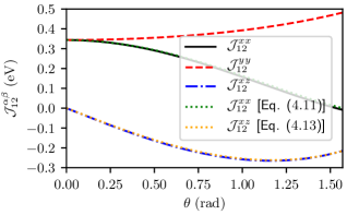
Figure 1: Comparison of the energy curvature components $\mathcal{J}_{12}^{xx}$ and $\mathcal{J}_{12}^{xz}$ of an Fe dimer [17] with results obtained from Eqs. (30-32) by setting $J_{12}=\mathcal{J}_{12}^{yy}$.

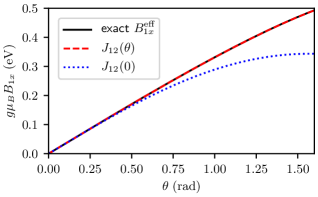
Figure 2: Comparison of the exact effective magnetic field $B_{1x}^{\text{eff}}$, acting on the first moment of an Fe dimer when the second moment is rotated by $\theta$ [17], with the effective field obtained from the effective exchange $J_{12}(\theta)$ and from the Heisenberg model with constant exchange $J_{12}(0)$.

When calculating the energy curvature tensor $\mathcal{J}_{ij}^{\alpha\beta}$ from the adiabatic energy (1), which produces an effective field that is perpendicular to the moment directions due to the minimization with respect to the moment lengths, it is not necessary to explicitly take the fixed unit length of the unit vectors $\mathbf{e}_{i}$ and $\mathbf{e}_{j}$ into account for $i\neq j$, i.e., it is allowed to just take the Cartesian derivatives with respect to the components $e_{i\alpha}$ and $e_{j\beta}$. This follows from the fact that the restriction of unit length is equivalent to setting the component of the gradient $\boldsymbol{\nabla}_{\mathbf{e}_{i}}$ parallel to $\mathbf{e}_{i}$ to zero, see Eq. (28). If the gradient of the energy has no such parallel component, it is therefore not necessary to apply this restriction. For the second derivative $\partial/\partial e_{j\beta}$, we have to project out the component parallel to $\mathbf{e}_{j}$,

$$\left.\boldsymbol{\nabla}_{\mathbf{e}_{j}}\frac{\partial E}{\partial e_{i\alpha}}\right|_{\perp} =\boldsymbol{\nabla}_{\mathbf{e}_{j}}\frac{\partial E}{\text{$\partial$}e_{i\alpha}}-\mathbf{e}_{j}\left(\mathbf{e}_{j}\cdot\boldsymbol{\nabla}_{\mathbf{e}_{j}}\frac{\partial E}{\partial e_{i\alpha}}\right).$$ (34)

For $i\neq j$, we can pull the derivative with respect to $e_{i\alpha}$ in front and use that $\mathbf{e}_{j}\cdot\boldsymbol{\nabla}_{\mathbf{e}_{j}}E=0$,

$$\left.\boldsymbol{\nabla}_{\mathbf{e}_{j}}\frac{\partial E}{\partial e_{i\alpha}}\right|_{\perp} \overset{i\neq j}{=}\boldsymbol{\nabla}_{\mathbf{e}_{j}}\frac{\partial E}{\partial e_{i\alpha}}-\frac{\partial}{\partial e_{i\alpha}}\mathbf{e}_{j}\left(\mathbf{e}_{j}\cdot\boldsymbol{\nabla}_{\mathbf{e}_{j}}E\right)$$

$$\overset{i\neq j}{=}\boldsymbol{\nabla}_{\mathbf{e}_{j}}\frac{\partial E}{\partial e_{i\alpha}}.$$ (35)

Therefore, the projection is then not required for $i\neq j$. This consideration does not apply to the tensorial Heisenberg model (21) and the exchange energy (23) above since the corresponding effective fields have a parallel component, which requires to take the restriction to unit length explicitly into account.

In summary, the effective exchange interaction $J_{ij}$ can be obtained from the following procedure:

1. Calculate the energy curvature tensor $\mathcal{J}_{ij}^{\alpha\beta}$.

2. For each pair $(i,j)$, rotate $\mathcal{J}_{ij}^{\alpha\beta}$ to the coordinate system where $\mathbf{e}_{i}=\hat{\mathbf{z}}$ and $\mathbf{e}_{j}$ lies in the $xz$ plane.

3. Set $J_{ij}=\mathcal{J}_{ij}^{yy}$.

V Tight-binding model

The tight-binding electronic structure model employed here is implemented in the software package Cahmd [45] and is based on a Hamiltonian that consists of a hopping term $\hat{\mathcal{H}}_{0}$, a local charge neutrality term $\hat{\mathcal{H}}_{\mathrm{lcn}}$, and a Stoner term $\hat{\mathcal{H}}_{\text{St}}$ [46, 47, 16],

$$\hat{\mathcal{H}}_{\mathrm{tb}}=\hat{\mathcal{H}}_{0}+\hat{\mathcal{H}}_{\mathrm{lcn}}+\hat{\mathcal{H}}_{\text{St}}.$$ (36)

The hopping term is in second-quantization given by

$$\hat{\mathcal{H}}_{0}=\sum_{i\ell,j\ell^{\prime},\sigma}t_{i\ell,j\ell^{\prime}}\hat{c}_{i\ell\sigma}^{\dagger}\hat{c}_{j\ell^{\prime}\sigma},$$ (37)

which describes the hopping of an electron from state $j\ell^{\prime}\sigma$ to $i\ell\sigma$ with hopping amplitude $t_{i\ell,j\ell^{\prime}}$ and creation and annihilation operators $\hat{c}_{i\ell\sigma}^{\dagger}$ and $\hat{c}_{j\ell^{\prime}\sigma}$. The index $i\ell\sigma$ indicates the lattice site, orbit, and spin, respectively. We use a Slater-Koster parameterization [48] of the hopping parameters in a non-orthognal basis which is based on Ref. [49]. It has been shown that such a tight-binding model provides a numerically efficient and valid description of transition metal elements and alloys [50] both for collinear and non-collinear magnetic configurations, based on comparisons with DFT calculations [51].

The local charge neutrality term is given by

$$\hat{\mathcal{H}}_{\text{lcn}} =\frac{1}{2}U_{\text{lcn}}\sum_{i}\left(\hat{n}_{i}-n_{i}^{0}\right)\left(\hat{n}_{i}-n_{i}^{0}\right)$$

$$\approx U_{\text{lcn}}\sum_{i}\hat{n}_{i}\left(n_{i}-n_{i}^{0}\right)+E_{\text{lcn}}^{\text{dc}},$$ (38)

where we apply a mean-field approximation and the double-counting contribution is

$$E_{\text{lcn}}^{\text{dc}}=-\frac{1}{2}U_{\text{lcn}}\sum_{i}\left[n_{i}^{2}-(n_{i}^{0})^{2}\right].$$ (39)

Here,

$$\hat{n}_{i}=\sum_{\ell\sigma}\hat{c}_{i\ell\sigma}^{\dagger}\hat{c}_{i\ell\sigma}$$ (40)

counts the number of electrons at site $i$ and $n_{i}^{0}$ is the prescribed number of electrons per site with $n_{i}=\langle\hat{n}_{i}\rangle$. The local charge neutrality term is similar to a Coulomb interaction and favors a charge-neutral state, which is exactly enforced in the limit $U_{\mathrm{lcn}}\to\infty$. In practice, $U_{\mathrm{lcn}}$ should be a large positive quantity [50, 51] and we use here $U_{\text{lcn}}=5\;\text{eV}$ [52, 47]. If all atoms are geometrically and chemically equivalent, the local charge neutrality term is only required for non-collinear magnetic configurations that break the equivalence. Finally, we describe the spin-splitting with a Stoner contribution $\hat{\mathcal{H}}_{\text{St}}$ to the Hamiltonian, which we discuss in Sec. V.1, and we explain the consequences for the calculation of the energy curvature tensor in Sec. V.2. We note that we do not include spin-orbit coupling in this work.

V.1 Stoner model

For the construction of the Stoner contribution $\hat{\mathcal{H}}_{\text{St}}$ to the Hamiltonian, it is crucial to ensure that

$$\left\langle\boldsymbol{\nabla}_{\mathbf{e}_{i}}\hat{\mathcal{H}}_{\text{St}}\right\rangle=0,$$ (41)

such that the energy is conserved. In some previous works [15, 17], a Stoner term of the following form was used,

$$\hat{\mathcal{H}}_{\text{St}}^{\text{old}}=-\frac{1}{2}\sum_{i\ell\ell^{\prime}}I_{\ell\ell^{\prime}}M_{i\ell}\mathbf{e}_{i}\cdot\hat{\mathbf{M}}_{i\ell^{\prime}},$$ (42)

where this requirement is not fulfilled and it is not possible to obtain a conserved total energy. Since we consider the conservation of energy as a necessary requirement for our spin dynamics simulations, we use instead the following Stoner term within a mean-field approximation [46, 47, 16],

$$\hat{\mathcal{H}}_{\text{St}} =-\frac{1}{4}\sum_{i\ell\ell^{\prime}}I_{\ell\ell^{\prime}}\hat{\mathbf{M}}_{i\ell}\cdot\hat{\mathbf{M}}_{i\ell^{\prime}}$$

$$\approx-\frac{1}{2}\sum_{i\ell\ell^{\prime}}I_{\ell\ell^{\prime}}\mathbf{M}_{i\ell}\cdot\hat{\mathbf{M}}_{i\ell^{\prime}}+E_{\text{St}}^{\text{dc}},$$ (43)

where the double-counting term is given by

$$E_{\text{St}}^{\text{dc}}=\frac{1}{4}\sum_{i\ell\ell^{\prime}}I_{\ell\ell^{\prime}}\mathbf{M}_{i\ell}\cdot\mathbf{M}_{i\ell^{\prime}}.$$ (44)

The inclusion of the energy contribution $E_{\text{St}}^{\text{dc}}$ is required to fulfill the condition $\langle\boldsymbol{\nabla}_{\mathbf{e}_{i}}\hat{\mathcal{H}}_{\text{St}}\rangle=0$.

V.2 Calculation of the energy curvature tensor

The procedure in Sec. IV.2 to obtain the effective exchange interaction $J_{ij}$ requires the energy curvature tensor $\mathcal{J}_{ij}^{\alpha\beta}$. For the calculation of $\mathcal{J}_{ij}^{\alpha\beta}$ within the above specified tight-binding description, we have to evaluate the gradient of the Stoner term, $\boldsymbol{\nabla}_{\mathbf{e}_{j}}\hat{\mathcal{H}}_{\text{St}}$, see Ref. [17] for details on the formalism. While this is straight-forward for the previous implementation, Eq. (42), in the case of our current implementation, Eq. (43), this involves the calculation of

$$\frac{\partial}{\partial e_{j\beta}}M_{i\ell\alpha}\approx M_{i\ell}\frac{\partial e_{i\alpha}}{\partial e_{j\beta}}=M_{i\ell}\delta_{ij}\delta_{\alpha\beta},$$ (45)

which we estimate by assuming that all orbital contributions point along the same direction, $\mathbf{M}_{i\ell}=M_{i\ell}\mathbf{e}_{i}$. Taking here the full derivative, ${\partial e_{i\alpha}}/{\partial e_{i\beta}}=\delta_{\alpha\beta}$, results in unphysical contributions to the energy gradient tensor which can be projected out and do not affect the physically relevant contributions [17]. We observe that the approximation in Eq. (45) does not result in accurate results when comparing the effective exchange $J_{ij}^{\text{c}}$ calculated from the energy curvature tensor given by Eq. (3.23) in Ref. [17] with the exchange obtained from the exact energy curvature tensor calculated by numerical differentiation of the constraining field. However, it turns out that an alternative result $J_{ij}^{\text{sc}}$ based on the curvature of the band energy, Eq. (3.28) in Ref. [17], which is analogous to Eq. (11) in Ref. [53], gives more accurate results within the approximation (45). For example, for the Fe chain discussed in Sec. VI.2, we obtain in the ferromagnetic ground state

$$J_{i,i+1}^{\text{exact}} =0.1298\;\text{eV},$$ (46)

$$J_{i,i+1}^{\text{c}} =0.1057\;\text{eV},$$ (47)

$$J_{i,i+1}^{\text{sc}} =0.1308\;\text{eV}.$$ (48)

Furthermore, in the case of an Fe dimer, we have also confirmed the reliability of $J_{ij}^{\text{sc}}$ in non-collinear configurations. Therefore, we will use in the following $J_{ij}^{\text{sc}}$ to provide an estimate of the exchange interaction $J_{ij}$. We note that more rigorous results could be achieved by calculating $\frac{\partial}{\partial e_{j\beta}}M_{i\ell\alpha}$ self-consistently together with the energy curvature tensor, which is beyond our current implementation.

VI Dynamics and effective exchange of spin-disordered states

VI.1 Fe, Co and Ni dimers

To test the tight-binding implementation of the Cahmd code [45], we have considered dimers of Fe, Co and Ni with a lattice constant of $2.0\,\mathrm{\textup{\AA}}$ and studied their dynamics. We took initially an angle of $\theta=20^{\circ}$, with $\theta$ being the angle between the magnetic moments, and performed the calculations with and without damping. The results without damping showed a good agreement with previous work [16], with the results shown in Fig. 3.

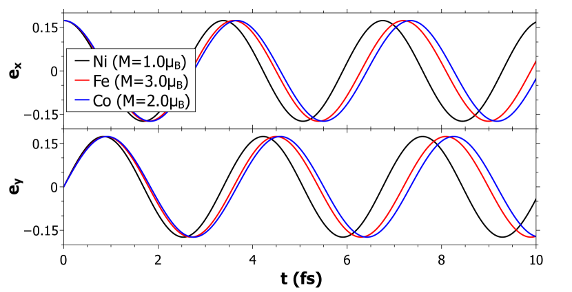
Figure 3: Time evolution of the magnetic moment components $e_{x}$ and $e_{y}$ for Ni, Fe and Co dimers (black, red and blue, respectively). Calculations are performed without damping. Note that since the calculation was performed without damping, the $z$ component of the magnetic moment is kept constant. The curves are for one atom. The other atom has an inverted dynamics due to the symmetry of the system.

For the systems with damping, we focused on the case of Fe. Here, we used a large damping $\alpha=0.5$ to let the system quickly relax to the ground state starting from different magnetic configurations (e.g., $\theta=20^{\circ}$, $\theta=80^{\circ}$ and $\theta=120^{\circ}$), as shown in Fig. 4. In the cases of $\theta=20^{\circ}$ and $\theta=80^{\circ}$, the dimer relaxed to a ferromagnetic (FM) state. For the angle $\theta=120^{\circ}$, the Fe dimer relaxed to the anti-ferromagnetic (AFM) configuration. This is in agreement with the sign of the exchange coupling parameter calculated for each starting configuration, see Fig. 5, as well as with the results shown in Ref. [16] where a stable ground state can be found around $\theta=180^{\circ}$.

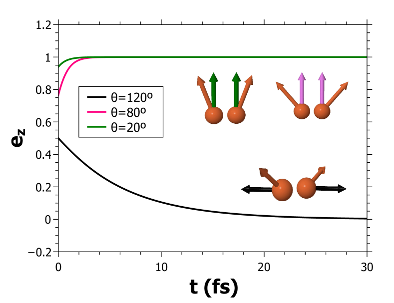
Figure 4: Time evolution of the $z$ component of the Fe dimer moment directions. Calculations were performed with the damping $\alpha=0.5$. The orange color of the atoms stands for the initial configuration whereas the different colored arrows represent the final configurations concerning their respective color in the legend.

Previous works have reported the nature of the AFM behavior of a few 3d metals by analyzing the different orbital-orbital contribution to the total exchange parameters in a crystal [54, 55], in particular Fe having a strong AF contribution coming from the T_2g-T_2g orbitals, therefore it is not surprising that the Fe dimer has a negative exchange coupling for a given magnetic configuration. In Fig. 5 one can see the dependence of the exchange parameter $J_{ij}$ as a function of the angle between the magnetic moments. Note that there is a discontinuity around 70 degrees and that is due to the abrupt change to the magnetic moment from approximately $3.0\;\mu_{B}$ for small angles to $1.22\;\mu_{B}$ at $\theta=120^{\circ}$, revealing the strong non-Heisenberg behavior for this system.

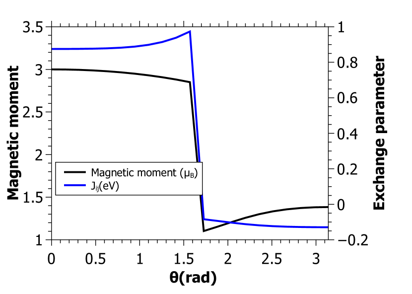
Figure 5: The calculated exchange parameter $J$ for different angles when varying a single magnetic moment in the Fe dimer (right axis) and the calculated magnetic moment for each one of these magnetic configurations (left axis).

Additionally, we also performed calculations for Fe and Co dimers using an orthogonal tight-binding basis, initially applied in Ref. [56]. The results (data not shown) show that the electronic structure is very similar to the one obtained using the non-orthogonal basis. This leads to similar exchange parameters and therefore similar dynamics of the magnetic moments compared to the ones presented in this section.

VI.2 Fe chain

We consider next the dynamics of an Fe spin chain with a lattice constant of $2.486\;\mathring{\mathrm{A}}$, which consists of $10$ atoms with periodic boundary conditions. We first check the analytical results on the conservation of energy and non-conservation of angular momentum by running a short $100\;\mathrm{fs}$ simulation without damping, starting from a randomly oriented spin configuration given by the maximally non-collinear configuration indicated in the inset of Fig. 10. Figure 6 shows that the change of the double counting contribution $E_{\text{dc}}$ compensates the change of the band energy $E_{\text{band}}$ such that the total energy is conserved within a numerical accuracy that depends on the chosen time step length. Here, with time steps of $0.1\;\mathrm{fs}$, the fluctuations are of the order of several $\mu\mathrm{eV}$. The non-conservation of angular momentum can be seen in Fig. 7, which shows the components of the total magnetization vector $\mathbf{M}$. We note that if we artificially constrain the moment lengths to a fixed value, angular momentum is conserved in our simulations as expected.

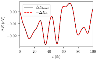
Figure 6: Time evolution of the change of the band energy ($\Delta E_{\text{band}}$) and double counting ($\Delta E_{\text{dc}}$) contributions to the total energy $E=E_{\text{band}}+E_{\text{dc}}$ of a 10 atom Fe spin chain in a non-collinear configuration without damping, demonstrating energy conservation.

Figure 7: Time evolution of the change $\Delta\mathbf{M}$ of the components of the total magnetization $\mathbf{M}$ of a 10 atom Fe spin chain from a non-collinear configuration without damping.

Next, we switch on a damping of $\alpha=0.01$ and let the spin chain relax. We track the nearest neighbor exchange interactions, magnetic moments, and energy, which are shown in Figs. 8 and 9, respectively. While the magnetic moments show only small flucuations of the order of 1%, the nearest neighbor exchange can vary by more than 50% and the average is increased by about 10% compared to the ferromagnetic ground state. Both energy and exchange are mostly relaxed after a simulation time of $4000\;\text{fs}$, but the individual magnetic moments still oscillate slowly and have not reached their ground-state value of $3.4\;\mu_{B}$.

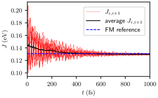
Figure 8: Relaxation of the nearest-neighbor exchange $J_{i,i+1}$ of a 10 atom Fe spin chain from a non-collinear configuration with damping $\alpha=0.01$.

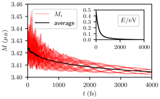
Figure 9: Relaxation of the magnetic moment lengths $M_{i}$ of a 10 atom Fe spin chain from a non-collinear configuration with damping $\alpha=0.01$. Inset: total energy $E$.

The Fe spin chain also allows to demonstrate the limitations of the effective exchange interaction in strongly non-collinear states due to multi-spin interactions that are not included in the two-spin exchange energy (23). In Fig. 10, we compare the exact effective field obtained from the constraining field with the effective field obtained from the exchange interaction $J_{ij}$ via Eqs. (27) and (28) under a continuous transformation of the moment directions from the ferromagnetic state to a random non-collinear state. Close to the collinear configuration, the agreement is nearly perfect both with the field obtained from $J_{ij}$ updated for each configuration and from constant $J_{ij}^{\mathrm{fm}}$ obtained from the ferromagnetic ground state. We find an improved agreement with the updated $J_{ij}$ over $J_{ij}^{\mathrm{fm}}$ for increasingly non-collinear states, but in strongly non-collinear states the effective exchange $J_{ij}$ is insufficient to obtain the correct effective field. This is different from the dimer case where the effective exchange gives the exact effective field. Therefore, we attribute this failure of the isotropic two-spin exchange to multi-spin interactions that are not included in an effective pair exchange formalism, since the isotropy could only be broken by spin-orbit coupling, which is not included in the tight-binding Hamiltonian (36) considered here.

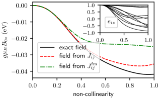
Figure 10: Comparison of the $z$ component of the exact effective field acting on the magnetic moment at site $i=0$ in a periodic 10 atom Fe spin chain with effective fields obtained from the effective exchange interaction $J_{ij}$ and its ferromagnetic ground-state value $J_{ij}^{\mathrm{fm}}$. The non-collinearity parameter describes a continuous transformation from a collinear state to a random non-collinear state, as illustrated in the inset by the $z$ components of the moment vectors $\mathbf{e}_{i}$.

VI.3 Co chain

We also investigated a chain of $10$ Co atoms along $x$ direction with a lattice constant of $2.50\,\mathrm{\textup{\AA}}$ in Fig. 11.

Figure 11: Time evolution of the normalized average magnetic moment $\bar{M}$ for $10$ atom chain of Co ($\bar{M}=1$ is the fully ferromagnetic state). The inset shows the spin configuration (black arrows) after equilibration.

The Gilbert damping is set to $0.05$ in order to guarantee fast relaxation from the initial random state, which is the same as for the Fe chain, see inset of Fig. 10. The magnetic moment length of each spin is $M=2.35\,\mathrm{\mu_{B}}$ and approximately constant during the relaxation process with a maximal deviation of $\Delta M=0.04\,\mathrm{\mu_{B}}$.

Surprisingly, the normalized magnetization relaxes not to a ferromagnetic but to a spiral state (see inset in Fig. 11), which does not depend on a particular choice of the damping parameter $\alpha$. From the total energy (per atom) of both the ferromagnetic state $E=3.558\,\mathrm{eV}$ and the spiral state $E=3.561\,\mathrm{eV}$ (so $\Delta E=3\,\mathrm{meV}=0.021J_{i,i+1}$), it is revealed that the spiral state is only metastable and not the ground state. Since the dynamics is driven by the exact effective field $\mathbf{B}_{i}^{\text{eff}}=-\mathbf{B}_{i}^{\text{con}}$, it is unclear which spin-spin exchange mechanism stabilizes the spiral state. Simulating the time-resolved Heisenberg exchange (Fig. 12) shows a strong ferromagnetic coupling between the nearest-neighbor magnetic moments ($J_{i,i+1}>0$); the second nearest-neighbor couplings are typically two-orders of magnitude smaller and antiferromagnetic ($J_{i,i+2}<0$). Spiral states in $3d$ transition metal chains have been previously reported [57, 58]. No spiral ground state was found for Co, but in the case of Fe a spiral state was obtained for lattice constants below the bulk value of $2.486\;\mathring{\mathrm{A}}$ and a ferromagnetic ground state for the bulk value [58], which is consistent with the result for the Fe chain above.

Figure 12: Relaxation of the nearest-neighbor exchange $J_{i,i+1}$ of a $10$ atom Co spin chain from a non-collinear configuration with damping $\alpha=0.05$.

Classical atomistic magnetization dynamics from a Heisenberg spin-Hamiltonian shows opposite to the tight-binding dynamics a relaxation to the ferromagnetic state (not shown here). Thus, the non-collinearity could result from multi-spin higher order exchange. To test this hypothesis, we compare the exact field (black line) with the effective field related to the Heisenberg spin-Hamiltonian (red line) in Fig. 13. Into the latter, the dynamically determined $J$’s enter.

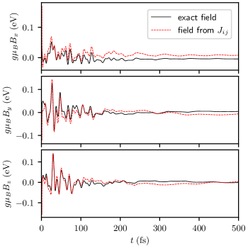
Figure 13: Dynamics of the exact effective field (black solid lines) and the effective field related to a Heisenberg spin-Hamiltonian with dynamical determined $J$’s (red dotted lines) for one atom in a chain of $10$ Co atoms. The different panels show the different Cartesian components of the fields.

There are clear deviations between the two fields, corroborating the presence of multi-spin exchange mechanisms. Unfortunately, there is no expression similar to the two-spin case [53, 17, 59] for multi-spin exchange interactions with constraining fields, which will be a focus of future studies.

VII Summary and discussion

In this work, we have considered adiabatic spin dynamics within a tight-binding electronic structure theory based on constraining fields. Furthermore, we have developed a method of extracting effective exchange interactions $J_{ij}$ from the energy curvature tensor $\mathcal{J}_{ij}^{\alpha\beta}$ in non-collinear configurations. The effective exchange goes beyond the simpler Heisenberg exchange, as it includes all contributions to the two-spin exchange interaction up to infinite order, resulting in an effective exchange interaction that depends on the magnetic configuration. Within the spin dynamics simulations, we can track the evolution of the effective exchange and its dependence on the magnetic configuration.

In particular, we considered Ni, Fe, and Co dimers, and Fe and Co spin chains consisting of ten atoms each. The results show that both moment lengths and effective exchange interactions depend dynamically on the magnetic configuration. For strongly non-collinear states in particular, the results demonstrate a breakdown of a Heisenberg model description, which assumes constant moment lengths and exchange interactions. In the case of the Fe chain, the magnetic moments only change by a few percent but the exchange interaction is strongly affected by non-collinearity, with an increase of the average nearest-neighbor exchange by about $10\;\%$ compared to the ferromagnetic ground state. For strongly non-collinear states, the two-spin exchange interaction is insufficient to obtain the correct effective field due to multi-spin interactions.

We have also shown that adiabatic spin dynamics at zero electronic temperature without any additional damping conserves the energy but not the total angular momentum. The adiabatic approximation implicitly introduces a coupling of the electronic system to a bath in order to keep the electrons in a quasi-equilibrium state. At zero temperature, heat cannot be transferred to the bath, $\delta Q=T\delta S=0$, which explains the conservation of energy despite the coupling to such a bath. Angular momentum, however, can be transferred even at zero temperature when the magnetic moment lengths are not constant. Our approach has the advantage that it includes the change of moment lengths in non-collinear configurations, which is a more accurate description of the physics than assuming constant moments. In any real system, the spin dynamics is coupled to the lattice, which allows a transfer of angular momentum between the lattice and the magnetic moments. The disadvantage of this adiabatic description is that it does not model this angular momentum transfer on a microscopic level and only takes it into account implicitly by a change of moment lengths without including the impact on the lattice. Future work will be required to establish how angular momentum conservation can be restored when including the lattice dynamics within this adiabatic framework.

As a final remark, we note that the conservation laws analyzed here in Sec. III, might have implications on how to interpret experimental pump-probe experiments, such as the ones published in Ref. [10]. The dynamics of the angular momentum of the electron system and its transfer to a bath is, according to this analysis, distinctly different for collinear and non-collinear systems. Even if the experiment is made for a system that initially is collinear, say a ferromagnet, any transient excited state that has a non-collinear magnetic structure will open up for new channels of angular momentum transfer, that could be relevant for how to understand these types of experiments. Further studies of the model presented here will hopefully clarify this point. To this end, it might be necessary to simulate directly the electron dynamics without adiabatic approximation, see, e.g., recent works on ultra-fast spin dynamics based on tight-binding models [60, 61].

Appendix A Derivative matrix

Naively, one would expect ${\partial e_{j\alpha}}/{\partial e_{j\beta}}=\delta_{\alpha\beta}$, which is however not valid for a unit vector since the Cartesian components are not independent. Instead, the derivative matrix evaluated at $\mathbf{e}_{j}=\sin\theta\,\mathbf{e}_{x}+\cos\theta\,\mathbf{e}_{z}$ is given by

$$\frac{\partial e_{j\alpha}}{\partial e_{j\beta}}=\begin{pmatrix}\cos^{2}\theta&0&-\sin\theta\cos\theta\\ 0&1&0\\ -\sin\theta\cos\theta&0&\sin^{2}\theta\end{pmatrix}_{\alpha\beta},$$ (49)

which we obtain from the gradient of a unit vector in spherical coordinates,

$$\boldsymbol{\nabla}_{\mathbf{e}_{j}}e_{j\alpha}(\theta,\phi)=\frac{\partial e_{j\alpha}}{\partial\theta}\mathbf{e}_{\theta}+\frac{1}{\sin\theta}\frac{\partial e_{j\alpha}}{\partial\phi}\mathbf{e}_{\phi},$$ (50)

with

$$\mathbf{e}_{j}=\begin{pmatrix}\sin\theta\cos\phi\\ \sin\theta\sin\phi\\ \cos\theta\end{pmatrix},$$ (51)

and

$$\mathbf{e}_{\theta} =\begin{pmatrix}\cos\theta\cos\phi\\ \cos\theta\sin\phi\\ -\sin\theta\end{pmatrix},\;\mathbf{e}_{\phi}=\begin{pmatrix}-\sin\phi\\ \cos\phi\\ 0\end{pmatrix}.$$ (52)

Appendix B Dzyaloshinskii–Moriya interaction

Here, we consider an additional DMI contribution to the generalized exchange in Sec. IV.1 [43, 44],

$$E_{\text{DMI}}=-\frac{1}{2}\sum_{ij}\mathbf{D}_{ij}\cdot\left(\mathbf{e}_{i}\times\mathbf{e}_{j}\right),$$ (53)

with $\mathbf{D}_{ij}=-\mathbf{D}_{ji}$ and $\mathbf{D}_{ii}=0$. Such a contribution is allowed if spin-orbit coupling is taken into account and inversion symmetry is broken. The DMI results in the following effective magnetic field in the reference coordinate system (with $\mathbf{e}_{i}=\hat{\mathbf{z}}$ and $\mathbf{e}_{j}$ in the $xz$ plane),

$$B_{ix}^{\text{eff}} =\frac{1}{M_{i}}\sum_{j}\left(D_{ij}^{z}e_{jy}-D_{ij}^{y}e{}_{jz}\right),$$ (54)

$$B_{iy}^{\text{eff}} =\frac{1}{M_{i}}\sum_{j}\left(-D_{ij}^{z}e_{jx}+D_{ij}^{x}e_{jz}\right),$$ (55)

$$B_{iz}^{\text{eff}} =0.$$ (56)

Combining the effective exchange and this DMI, we obtain in the reference coordinate system (for $i\neq j$)

$$\mathcal{J}_{ij}^{xx} = J_{ij}(\theta_{ij})\cos^{2}\theta_{ij}$$ (57)

$$+\sin\theta_{ij}\cos\theta_{ij}\left(J^{\prime}_{ij}(\theta_{ij})+D_{ij}^{y}\right),$$

$$\mathcal{J}_{ij}^{xy} = D_{ij}^{z},$$ (58)

$$\mathcal{J}_{ij}^{xz} = -J_{ij}(\theta_{ij})\sin\theta_{ij}\cos\theta_{ij}$$ (59)

$$-\sin^{2}\theta_{ij}\left(J^{\prime}_{ij}(\theta_{ij})+D_{ij}^{y}\right),$$

$$\mathcal{J}_{ij}^{yx} = -D_{ij}^{z}\cos^{2}\theta_{ij}-D_{ij}^{x}\sin\theta_{ij}\cos\theta_{ij},$$ (60)

$$\mathcal{J}_{ij}^{yy} = J_{ij}(\theta_{ij}),$$ (61)

$$\mathcal{J}_{ij}^{yz} = D_{ij}^{x}\sin^{2}\theta_{ij}+D_{ij}^{z}\sin\theta_{ij}\cos\theta_{ij},$$ (62)

$$\mathcal{J}_{ij}^{z\beta} = 0.$$ (63)

We note that the contributions with $J^{\prime}_{ij}(\theta_{ij})$ and $D_{ij}^{y}$ cannot be distinguished here from a single configuration and they both change sign under exchange $i\leftrightarrow j$, see Eq. (29). From a collinear state aligned along the $z$ axis, we can obtain the components $D_{ij}^{z}$ of the DMI, in agreement with Ref. [42].

References

- Antropov et al. [1995] V. P. Antropov, M. I. Katsnelson, M. van Schilfgaarde, and B. N. Harmon, Spin Dynamics in Magnets, Phys. Rev. Lett. 75, 729 (1995).
- Antropov et al. [1996] V. P. Antropov, M. I. Katsnelson, B. N. Harmon, M. van Schilfgaarde, and D. Kusnezov, Spin dynamics in magnets: Equation of motion and finite temperature effects, Phys. Rev. B 54, 1019 (1996).
- Halilov et al. [1998] S. V. Halilov, H. Eschrig, A. Y. Perlov, and P. M. Oppeneer, Adiabatic spin dynamics from spin-density-functional theory: Application to Fe, Co, and Ni, Phys. Rev. B 58, 293 (1998).
- Stocks et al. [1998] G. M. Stocks, B. Ujfalussy, X. Wang, D. M. C. Nicholson, W. A. Shelton, Y. Wang, A. Canning, and B. L. Györffy, Towards a constrained local moment model for first principles spin dynamics, Philos. Mag. B 78, 665 (1998).
- Ujfalussy et al. [1999] B. Ujfalussy, X.-D. Wang, D. M. C. Nicholson, W. A. Shelton, G. M. Stocks, Y. Wang, and B. L. Gyorffy, Constrained density functional theory for first principles spin dynamics, J. Appl. Phys. 85, 4824 (1999).
- Ma and Dudarev [2015] P.-W. Ma and S. L. Dudarev, Constrained density functional for noncollinear magnetism, Phys. Rev. B 91, 054420 (2015).
- Singer et al. [2005] R. Singer, M. Fähnle, and G. Bihlmayer, Constrained spin-density functional theory for excited magnetic configurations in an adiabatic approximation, Phys. Rev. B 71, 214435 (2005).
- Bertotti et al. [2009] G. Bertotti, I. D. Mayergoyz, and C. Serpico, Nonlinear Magnetization Dynamics in Nanosystems (Elsevier, Oxford, 2009).
- Eriksson et al. [2017] O. Eriksson, A. Bergman, L. Bergqvist, and J. Hellsvik, Atomistic Spin Dynamics: Foundations and Applications (Oxford University Press, 2017).
- Beaurepaire et al. [1996] E. Beaurepaire, J.-C. Merle, A. Daunois, and J.-Y. Bigot, Ultrafast spin dynamics in ferromagnetic nickel, Phys. Rev. Lett. 76, 4250 (1996).
- Böttcher et al. [2012] D. Böttcher, A. Ernst, and J. Henk, Temperature-dependent Heisenberg exchange coupling constants from linking electronic-structure calculations and Monte Carlo simulations, J. Magn. Magn. Mater. 324, 610 (2012).
- Mankovsky et al. [2013] S. Mankovsky, S. Polesya, H. Ebert, W. Bensch, O. Mathon, S. Pascarelli, and J. Minár, Pressure-induced bcc to hcp transition in Fe: Magnetism-driven structure transformation, Phys. Rev. B 88, 184108 (2013).
- Mankovsky et al. [2020a] S. Mankovsky, S. Polesya, and H. Ebert, Exchange coupling constants at finite temperature, Phys. Rev. B 102, 134434 (2020a).
- Rózsa et al. [2014] L. Rózsa, L. Udvardi, and L. Szunyogh, Langevin spin dynamics based on ab initio calculations: numerical schemes and applications, J. Phys. Condens. Matter 26, 216003 (2014).
- Streib et al. [2020] S. Streib, V. Borisov, M. Pereiro, A. Bergman, E. Sjöqvist, A. Delin, O. Eriksson, and D. Thonig, Equation of motion and the constraining field in ab initio spin dynamics, Phys. Rev. B 102, 214407 (2020).
- Cardias et al. [2021] R. Cardias, C. Barreteau, P. Thibaudeau, and C. C. Fu, Spin dynamics from a constrained magnetic tight-binding model, Phys. Rev. B 103, 235436 (2021).
- Streib et al. [2021] S. Streib, A. Szilva, V. Borisov, M. Pereiro, A. Bergman, E. Sjöqvist, A. Delin, M. I. Katsnelson, O. Eriksson, and D. Thonig, Exchange constants for local spin Hamiltonians from tight-binding models, Phys. Rev. B 103, 224413 (2021).
- Antropov et al. [1997] V. Antropov, M. Katsnelson, and A. Liechtenstein, Exchange interactions in magnets, Physica B Condens. Matter 237-238, 336 (1997).
- Antropov et al. [1999] V. Antropov, B. Harmon, and A. Smirnov, Aspects of spin dynamics and magnetic interactions, J. Magn. Magn. Mater. 200, 148 (1999).
- Szilva et al. [2013] A. Szilva, M. Costa, A. Bergman, L. Szunyogh, L. Nordström, and O. Eriksson, Interatomic Exchange Interactions for Finite-Temperature Magnetism and Nonequilibrium Spin Dynamics, Phys. Rev. Lett. 111, 127204 (2013).
- Secchi et al. [2015] A. Secchi, A. Lichtenstein, and M. Katsnelson, Magnetic interactions in strongly correlated systems: Spin and orbital contributions, Ann. Phys. (N. Y.) 360, 61 (2015).
- Szilva et al. [2017] A. Szilva, D. Thonig, P. F. Bessarab, Y. O. Kvashnin, D. C. M. Rodrigues, R. Cardias, M. Pereiro, L. Nordström, A. Bergman, A. B. Klautau, and O. Eriksson, Theory of noncollinear interactions beyond Heisenberg exchange: Applications to bcc Fe, Phys. Rev. B 96, 144413 (2017).
- Cardias et al. [2020a] R. Cardias, A. Szilva, M. M. Bezerra-Neto, M. S. Ribeiro, A. Bergman, Y. O. Kvashnin, J. Fransson, A. B. Klautau, O. Eriksson, and L. Nordström, First-principles Dzyaloshinskii–Moriya interaction in a non-collinear framework, Sci. Rep. 10, 20339 (2020a).
- Cardias et al. [2020b] R. Cardias, A. Bergman, A. Szilva, Y. O. Kvashnin, J. Fransson, A. B. Klautau, O. Eriksson, and L. Nordström, Dzyaloshinskii-Moriya interaction in absence of spin-orbit coupling (2020b), arXiv:2003.04680 .
- Tanaka and Uryû [1977] Y. Tanaka and N. Uryû, Exchange Interactions in Antiferromagnetic FeI2. II. The Four Spin Interaction, J. Phys. Soc. Jpn. 43, 1569 (1977).
- MacDonald et al. [1988] A. H. MacDonald, S. M. Girvin, and D. Yoshioka, expansion for the Hubbard model, Phys. Rev. B 37, 9753 (1988).
- Singer et al. [2011] R. Singer, F. Dietermann, and M. Fähnle, Spin Interactions in bcc and fcc Fe beyond the Heisenberg Model, Phys. Rev. Lett. 107, 017204 (2011).
- Hoffmann and Blügel [2020] M. Hoffmann and S. Blügel, Systematic derivation of realistic spin models for beyond-Heisenberg solids, Phys. Rev. B 101, 024418 (2020).
- Brinker et al. [2020] S. Brinker, M. dos Santos Dias, and S. Lounis, Prospecting chiral multisite interactions in prototypical magnetic systems, Phys. Rev. Research 2, 033240 (2020).
- Mankovsky et al. [2020b] S. Mankovsky, S. Polesya, and H. Ebert, Extension of the standard Heisenberg Hamiltonian to multispin exchange interactions, Phys. Rev. B 101, 174401 (2020b).
- Antropov [2003] V. Antropov, The exchange coupling and spin waves in metallic magnets: removal of the long-wave approximation, J. Magn. Magn. Mater. 262, L192 (2003).
- Katsnelson and Lichtenstein [2004] M. I. Katsnelson and A. I. Lichtenstein, Magnetic susceptibility, exchange interactions and spin-wave spectra in the local spin density approximation, J. Phys. Condens. Matter 16, 7439 (2004).
- Buczek et al. [2011] P. Buczek, A. Ernst, and L. M. Sandratskii, Different dimensionality trends in the Landau damping of magnons in iron, cobalt, and nickel: Time-dependent density functional study, Phys. Rev. B 84, 174418 (2011).
- Durhuus et al. [2022] F. Durhuus, T. Skovhus, and T. Olsen, Plane wave implementation of the magnetic force theorem for magnetic exchange constants: Application to bulk Fe, Co and Ni (2022), arXiv:2204.04169 .
- Landau and Lifshitz [1977] L. D. Landau and E. M. Lifshitz, Quantum Mechanics, Non-Relativistic Theory, 3rd ed. (Pergamon Press, Oxford, 1977).
- Töws and Pastor [2015] W. Töws and G. M. Pastor, Many-body theory of ultrafast demagnetization and angular momentum transfer in ferromagnetic transition metals, Phys. Rev. Lett. 115, 217204 (2015).
- Gilbert [2004] T. L. Gilbert, A phenomenological theory of damping in ferromagnetic materials, IEEE Trans. Magn. 40, 3443 (2004).
- Mentink et al. [2010] J. H. Mentink, M. V. Tretyakov, A. Fasolino, M. I. Katsnelson, and T. Rasing, Stable and fast semi-implicit integration of the stochastic Landau–Lifshitz equation, J. Phys. Condens. Matter 22, 176001 (2010).
- Yuan et al. [2014] Z. Yuan, K. M. D. Hals, Y. Liu, A. A. Starikov, A. Brataas, and P. J. Kelly, Gilbert damping in noncollinear ferromagnets, Phys. Rev. Lett. 113, 266603 (2014).
- Mankovsky et al. [2018] S. Mankovsky, S. Wimmer, and H. Ebert, Gilbert damping in noncollinear magnetic systems, Phys. Rev. B 98, 104406 (2018).
- Brinker et al. [2022] S. Brinker, M. dos Santos Dias, and S. Lounis, Generalization of the Landau-Lifshitz-Gilbert equation by multi-body contributions to Gilbert damping for non-collinear magnets (2022), arXiv:2202.06154 .
- Udvardi et al. [2003] L. Udvardi, L. Szunyogh, K. Palotás, and P. Weinberger, First-principles relativistic study of spin waves in thin magnetic films, Phys. Rev. B 68, 104436 (2003).
- Dzyaloshinsky [1958] I. Dzyaloshinsky, A thermodynamic theory of “weak” ferromagnetism of antiferromagnetics, J. Phys. Chem. Solids 4, 241 (1958).
- Moriya [1960] T. Moriya, Anisotropic superexchange interaction and weak ferromagnetism, Phys. Rev. 120, 91 (1960).
- [45] Computer code CAHMD, classical atomistic hybrid multi-degree dynamics. A computer program package for atomistic dynamics simulations of multiple degrees of freedom (e.g. electron, magnetization, lattice vibrations) based on parametrized Hamiltonians. (Danny Thonig, danny.thonig@oru.se, 2013) (unpublished, available from https://cahmd.gitlab.io/cahmdweb/).
- Autès et al. [2006] G. Autès, C. Barreteau, D. Spanjaard, and M.-C. Desjonquères, Magnetism of iron: from the bulk to the monatomic wire, J. Phys. Condens. Matter 18, 6785 (2006).
- Rossen [2019] S. Rossen, Magnetization disorder at finite temperature: A tight-binding Monte Carlo modelling and spin dynamics study of bulk iron and cobalt clusters: theory, numerical implementation and simulations, Ph.D. thesis, Radboud University Nijmegen (2019).
- Slater and Koster [1954] J. C. Slater and G. F. Koster, Simplified LCAO Method for the Periodic Potential Problem, Phys. Rev. 94, 1498 (1954).
- Mehl and Papaconstantopoulos [1996] M. J. Mehl and D. A. Papaconstantopoulos, Applications of a tight-binding total-energy method for transition and noble metals: Elastic constants, vacancies, and surfaces of monatomic metals, Phys. Rev. B 54, 4519 (1996).
- Barreteau et al. [2016] C. Barreteau, D. Spanjaard, and M.-C. Desjonquères, An efficient magnetic tight-binding method for transition metals and alloys, C. R. Phys. 17, 406 (2016).
- Soulairol et al. [2016] R. Soulairol, C. Barreteau, and C.-C. Fu, Interplay between magnetism and energetics in Fe-Cr alloys from a predictive noncollinear magnetic tight-binding model, Phys. Rev. B 94, 024427 (2016).
- Schena [2010] T. Schena, Tight-Binding Treatment of Complex Magnetic Structures in Low-Dimensional Systems, Diploma thesis, TH Aachen (2010).
- Bruno [2003] P. Bruno, Exchange interaction parameters and adiabatic spin-wave spectra of ferromagnets: A “renormalized magnetic force theorem”, Phys. Rev. Lett. 90, 087205 (2003).
- Kvashnin et al. [2016] Y. O. Kvashnin, R. Cardias, A. Szilva, I. Di Marco, M. I. Katsnelson, A. I. Lichtenstein, L. Nordström, A. B. Klautau, and O. Eriksson, Microscopic Origin of Heisenberg and Non-Heisenberg Exchange Interactions in Ferromagnetic bcc Fe, Phys. Rev. Lett. 116, 217202 (2016).
- Cardias et al. [2017] R. Cardias, A. Szilva, A. Bergman, I. D. Marco, M. I. Katsnelson, A. I. Lichtenstein, L. Nordström, A. B. Klautau, O. Eriksson, and Y. O. Kvashnin, The Bethe-Slater curve revisited; new insights from electronic structure theory, Sci. Rep. 7, 4058 (2017).
- Thonig and Henk [2014] D. Thonig and J. Henk, Gilbert damping tensor within the breathing Fermi surface model: anisotropy and non-locality, New J. Phys 16, 013032 (2014).
- Tung and Guo [2011] J. C. Tung and G. Y. Guo, Ab initio studies of spin-spiral waves and exchange interactions in transition metal atomic chains, Phys. Rev. B 83, 144403 (2011).
- Töws and Pastor [2012] W. Töws and G. M. Pastor, Theoretical study of the temperature dependence of the magnon dispersion relation in transition-metal wires and monolayers, Phys. Rev. B 86, 054443 (2012).
- Solovyev [2021] I. V. Solovyev, Exchange interactions and magnetic force theorem, Phys. Rev. B 103, 104428 (2021).
- Toepler et al. [2021] F. Toepler, J. Henk, and I. Mertig, Ultrafast spin dynamics in inhomogeneous systems: a density-matrix approach applied to Co/Cu interfaces, New J. Phys 23, 033042 (2021).
- Hamamera et al. [2022] H. Hamamera, F. S. M. Guimarães, M. dos Santos Dias, and S. Lounis, Polarisation-dependent single-pulse ultrafast optical switching of an elementary ferromagnet, Commun. Phys. 5, 16 (2022).