Bounds on Wasserstein distances between continuous distributions using independent samples

Tamás Papp1 t.papp@lancaster.ac.uk    Chris Sherlock2
1STOR-i CDT, Lancaster University, UK
2Department of Mathematics and Statistics, Lancaster University, UK
Abstract

The plug-in estimator of the Wasserstein distance is known to be conservative, however its usefulness is severely limited when the distributions are similar as its bias does not decay to zero with the true Wasserstein distance. We propose a linear combination of plug-in estimators for the squared 2-Wasserstein distance with a reduced bias that decays to zero with the true distance. The new estimator is provably conservative provided one distribution is appropriately overdispersed with respect the other, and is unbiased when the distributions are equal. We apply it to approximately bound from above the 2-Wasserstein distance between the target and current distribution in Markov chain Monte Carlo, running multiple identically distributed chains which start, and remain, overdispersed with respect to the target. Our bound consistently outperforms the current state-of-the-art bound, which uses coupling, improving mixing time bounds by up to an order of magnitude.

Keywords: jackknife estimator of variance, Markov chain Monte Carlo, optimal transport, stochastic ordering, Wasserstein distance.

1 Introduction

Wasserstein distances (villani2009optimal) are a class of metrics between probability measures, which have found extensive use in probability (villani2003topics; villani2009optimal), statistics (panaretos2019statistical; ramdas2019on), and machine learning (arjovsky2017wasserstein; peyre2019computational). Wasserstein distances metrize weak convergence, and have been used in Markov chain Monte Carlo to theoretically assess the convergence of sampling algorithms to their stationary distribution and the asymptotic bias of approximate sampling algorithms (durmus2019high; durmus2021asymptotic).

Wasserstein distances are analytically intractable for all but a few special cases. In practice, one can estimate them from a plug-in estimator constructed using independent samples from the distributions of interest. While relatively well-behaved in the discrete case (sommerfeld2018inference; tameling2019empirical), the plug-in estimator suffers from the curse of dimensionality in the continuous case, with its rate of decay with the sample size worsening exponentially as the dimension of the problem increases (fournier2015on; weed2019sharp; chizat2020faster). This translates into a significant upward bias for all but extremely large sample sizes. Worse, the plug-in estimator essentially attains a minimax optimal rate of convergence without additional assumptions beyond continuity (niles-weed2019estimation).

Thus, a search for a general estimator which decays more quickly as the number of samples increases would be futile. Instead, we aim to obtain consistent estimators which are additionally meaningful bounds on the distance, especially as the distance shrinks. We achieve this by linearly combining plug-in estimators, in essence subtracting off a large portion of the bias of the plug-in estimator. We characterize when it is possible to do so and still obtain an upper bound in expectation, and we show that is straightforward to obtain an estimator of a lower bound in expectation. Our bounds converge no slower than the plug-in estimators they partially debias, and we show that the probability that the point estimators of our bounds are not themselves bounds decays exponentially with the sample size. We also propose an algorithm to compute the jackknife variance estimator of our bounds, which enables uncertainty quantification at no increase in computational complexity with the sample size, relative to solving for the bounds exactly.

An attractive feature of our upper and lower bound estimators is that, in contrast with the plug-in estimator, whatever the sample size, their biases decrease in proportion to the Wasserstein distance itself. We therefore apply our bounds to Markov chain Monte Carlo, quantifying the convergence of Markov chains in Wasserstein distance through direct empirical estimates. The idea is to run several independent and identically distributed Markov chains until convergence, and to graph the plug-in estimator of the squared 2-Wasserstein distance between the marginal distributions and stationary distribution. If the chains are started overdispersed with respect to the target and stay so until convergence, one can subtract off the asymptote in the graph and obtain an upper bound on the squared distance whose expectation decays to zero when the chains converge. The analogous procedure on the scale of the Wasserstein distance, instead of its square, achieves a lower bound on the distance. In effect, one backtracks and declares convergence when the asymptote occurs, similarly to the popular potential scale reduction factor R^^𝑅\widehat{R} (gelman1992inference; brooks1998general; vehtari2021rank-normalization). We believe that our bounds will prove useful to compare the convergence of different Markov chains targeting the same stationary distribution, and to complement theoretical studies on Markov chain convergence with numerical results.

More closely related to our proposed bounds is the L𝐿L-lag coupling upper bound proposed in biswas2019estimating, which can also be used to quantify the convergence of Markov chains. The bound applies to a certain class of integral probability metrics (sriperumbudur2012on) including the total variation distance and the 1-Wasserstein distance. The methodology can however be extended straightforwardly to 2-Wasserstein distances, and so can be directly compared to our bounds. Similarities between our bounds and the coupling bound include the use of many identically distributed Markov chains, and the eventual decay of the bounds towards zero as the chains converge. As opposed to our bounds, the coupling bound does not require overdispersion, and applies to discretely supported measures as well. At the same time, the coupling bound is not a consistent estimator, and need not decay in proportion to the true distance it bounds. As we show in the simulations of Section 4.4, even state-of-the art couplings can be sub-optimal to a large extent, making the coupling bound very loose in comparison to our empirical bounds.

1.1 Wasserstein distances

Let (d,)superscript𝑑delimited-∥∥(\mathbb{R}^{d},\lVert\cdot\rVert) be the d𝑑d-dimensional real space endowed with the usual Euclidean norm. For two Borel probability measures μ,ν𝜇𝜈\mu,\nu on dsuperscript𝑑\mathbb{R}^{d}, the Wasserstein distance of order 222, or 222-Wasserstein distance is

𝒲2(μ,ν)=(inf(X,Y)Γ(μ,ν)𝔼XY2)1/2,subscript𝒲2𝜇𝜈superscriptsubscriptinfimum𝑋𝑌Γ𝜇𝜈𝔼superscriptdelimited-∥∥𝑋𝑌212\mathcal{W}_{2}(\mu,\nu)=\left(\inf_{(X,Y)\in\Gamma(\mu,\nu)}\mathbb{E}\lVert X-Y\rVert^{2}\right)^{1/2},

where Γ(μ,ν)Γ𝜇𝜈\Gamma(\mu,\nu) is the set of all couplings, that is probability measures in 𝒫(d×d)𝒫superscript𝑑superscript𝑑\mathcal{P}(\mathbb{R}^{d}\times\mathbb{R}^{d}) with marginals μ,ν𝜇𝜈\mu,\nu. The Wasserstein distance defines a metric on the space of probability measures with finite second moment. Convergence in the Wasserstein distribution is equivalent to convergence in distribution alongside convergence in the second moment (villani2009optimal).

There exists a unique optimal coupling π𝜋\pi of μ,ν𝜇𝜈\mu,\nu (villani2009optimal, Theorem 4.1). Under suitable regularity conditions on the distributions μ,ν𝜇𝜈\mu,\nu, for instance if both are continuous (brenier1991polar; mccann1995existence), there exists an optimal transport map T𝑇T which pushes forward μ𝜇\mu to ν𝜈\nu, such that

𝒲2(μ,ν)=(𝔼μXT(X)2)1/2.subscript𝒲2𝜇𝜈superscriptsubscript𝔼𝜇superscriptdelimited-∥∥𝑋𝑇𝑋212\mathcal{W}_{2}(\mu,\nu)=\left(\mathbb{E}_{\mu}\lVert X-T(X)\rVert^{2}\right)^{1/2}.

If μ𝜇\mu and ν𝜈\nu are continuous, then T=φ𝑇𝜑T=\nabla\varphi uniquely (dμd𝜇\mathrm{d}\mu-almost everywhere) for a convex function φ:d:𝜑superscript𝑑\varphi:\mathbb{R}^{d}\to\mathbb{R} called the Brenier potential from μ𝜇\mu to ν𝜈\nu. Conversely, there exists a convex φ~:d:~𝜑superscript𝑑\tilde{\varphi}:\mathbb{R}^{d}\to\mathbb{R} such that the optimal transport map from ν𝜈\nu to μ𝜇\mu is T1=φ~superscript𝑇1~𝜑T^{-1}=\nabla\tilde{\varphi} uniquely (dνd𝜈\mathrm{d}\nu-almost everywhere), and φ~~𝜑\tilde{\varphi} is the associated Brenier potential from ν𝜈\nu to μ𝜇\mu. See Appendix A for a precise statement and additional background on optimal transport and convexity.

For ease of exposition, we avoid presenting p𝑝p-Wasserstein distances with exponents p2𝑝2p\neq 2 and general transportation costs in the main body of this work. We however introduce these concepts in the supplementary material. This is both to explain how certain results, such as the lower bound (2), generalize, as well as to aid in the proofs.

1.1.1 Empirical Wasserstein distance

Let μ^nsubscript^𝜇𝑛\hat{\mu}_{n}, ν^nsubscript^𝜈𝑛\hat{\nu}_{n} be independent empirical measures, each comprising of n𝑛n equally weighted independent samples with weight 1/n1𝑛1/n. Based on μ^nsubscript^𝜇𝑛\hat{\mu}_{n} and ν^nsubscript^𝜈𝑛\hat{\nu}_{n}, the empirical Wasserstein distance between μ𝜇\mu and ν𝜈\nu is 𝒲2(μ^n,ν^n)subscript𝒲2subscript^𝜇𝑛subscript^𝜈𝑛\mathcal{W}_{2}(\hat{\mu}_{n},\hat{\nu}_{n}). We briefly summarize theoretical and computational properties of this plug-in estimator; see the review panaretos2019statistical for an overview of statistical aspects, and the monograph peyre2019computational for computational aspects.

The empirical Wasserstein distance is known to be consistent, converging almost surely to 𝒲2(μ,ν)subscript𝒲2𝜇𝜈\mathcal{W}_{2}(\mu,\nu) as n𝑛n\to\infty (villani2009optimal, Corollary 6.11). When μ,ν𝜇𝜈\mu,\nu are both discrete, the estimator is well-behaved (see sommerfeld2018inference; tameling2019empirical, for limit theorems). The one-dimensional continuous case is also well-behaved, see the review of bobkov2019one-dimensional for rates of mean-convergence, and delbarrio2005asymptotics; delbarrio2019a for limit theorems. Whether μ,ν𝜇𝜈\mu,\nu are continuous or discrete, the computation of 𝒲2(μ^n,ν^n)subscript𝒲2subscript^𝜇𝑛subscript^𝜈𝑛\mathcal{W}_{2}(\hat{\mu}_{n},\hat{\nu}_{n}) is straightforward in the one-dimensional case, with the optimal coupling being a pairing of order statistics, for O(nlogn)𝑂𝑛𝑛O(n\log n) cost.

Our focus is on the moderate-to-high dimensional continuous setting, when the plug-in estimator is known to suffer from the curse of dimensionality (fournier2015on; weed2019sharp; chizat2020faster). The estimator however concentrates well around its mean (weed2019sharp; chizat2020faster), obeying a central limit theorem (delbarrio2019central; delbarrio2019a; delbarrio2021central) under minor regularity assumptions.

In general, one can compute the empirical Wasserstein distance by solving a linear program, for which exact O~(n3)~𝑂superscript𝑛3\widetilde{O}(n^{3}) algorithms exist, where the notation O~~𝑂\widetilde{O} obscures logarithmic factors. Interpreting the problem as one of optimal assignment, one could use the classical Hungarian algorithm (kuhn1955the; see the discussions in jonker1984improving, jonker1987a, crouse2016on for optimizations). However, algorithms which are tailored to the more general optimization problem of finding the minimum cost flow in a network are often more efficient in practice (see kovacs2015minimum-cost, for a comprehensive discussion). Our experiments are in the moderate sample size regime (up to n=1000𝑛1000n=1000), where exact computations are feasible, and so we employ exact solvers throughout. The cubic complexity of exact algorithms may however be prohibitive for large instances n𝑛n. In such scenarios, one might consider targeting an entropically regularized version of the transportation cost instead. This offers both computational and statistical advantages (cuturi2013sinkhorn; mena2019statstical), although the entropic estimator is no longer consistent for the transportation cost.

1.2 Overview of results

1.2.1 Bounds

We informally describe out main results. For continuous measures μ𝜇\mu and ν𝜈\nu with ν𝜈\nu overdispersed (see below) with respect to μ𝜇\mu, let ν^nsubscript^𝜈𝑛\hat{\nu}_{n}, μ^nsubscript^𝜇𝑛\hat{\mu}_{n} and μ^nsuperscriptsubscript^𝜇𝑛\hat{\mu}_{n}^{\prime} be independent samples of size n𝑛n from ν𝜈\nu, μ𝜇\mu and μ𝜇\mu respectively. Theorem 1 essentially states that

𝔼[𝒲22(ν^n,μ^n)𝒲22(μ^n,μ^n)]𝒲22(μ,ν).𝔼delimited-[]superscriptsubscript𝒲22subscript^𝜈𝑛subscript^𝜇𝑛superscriptsubscript𝒲22subscriptsuperscript^𝜇𝑛subscript^𝜇𝑛superscriptsubscript𝒲22𝜇𝜈\mathbb{E}\big{[}\mathcal{W}_{2}^{2}(\hat{\nu}_{n},\hat{\mu}_{n})-\mathcal{W}_{2}^{2}(\hat{\mu}^{\prime}_{n},\hat{\mu}_{n})\big{]}\geq\mathcal{W}_{2}^{2}(\mu,\nu). (1)

Our sufficient condition, informally termed “overdispersed”, asks for the optimal transport map from ν𝜈\nu to μ𝜇\mu to be 1-Lipschitz. We refer to this as contractive optimal transport. If ν𝜈\nu and μ𝜇\mu differ only by a shift in mean, equality is attained in (1). As ν𝜈\nu approaches μ𝜇\mu, the left-hand side of equation (1) decays in proportion to 𝒲2(μ,ν)subscript𝒲2𝜇𝜈\mathcal{W}_{2}(\mu,\nu). As a converse to the upper bound, if ν𝜈\nu is underdispersed with respect to μ𝜇\mu, the reverse inequality holds. Further, assuming only that the samples are independent, it holds that

|𝔼[𝒲2(ν^n,μ^n)𝒲2(μ^n,μ^n)]|𝒲2(μ,ν).𝔼delimited-[]subscript𝒲2subscript^𝜈𝑛subscript^𝜇𝑛subscript𝒲2subscriptsuperscript^𝜇𝑛subscript^𝜇𝑛subscript𝒲2𝜇𝜈\big{|}\mathbb{E}\big{[}\mathcal{W}_{2}(\hat{\nu}_{n},\hat{\mu}_{n})-\mathcal{W}_{2}(\hat{\mu}^{\prime}_{n},\hat{\mu}_{n})\big{]}\big{|}\leq\mathcal{W}_{2}(\mu,\nu). (2)

We apply our bounds to estimate, from samples, the convergence in Wasserstein distance of a Markov chain targeting a continuous distribution. Multiple independent and identically distributed copies of the chain are started from a distribution π0subscript𝜋0\pi_{0} which is overdispersed with respect to the stationary distribution πsubscript𝜋\pi_{\infty}, and run until they each approximately draw at least two independent samples from the stationary distribution πsubscript𝜋\pi_{\infty}. Let πtsubscript𝜋𝑡\pi_{t} denote the marginal distribution of the chain at time t𝑡t. Plotting the squared Wasserstein distance between the samples at iterations t0𝑡0t\geq 0 and a collection of samples which are approximately from the stationary distribution will reveal an asymptote. Subtracting off the asymptote yields an estimate of the upper bound (1) on 𝒲22(πt,π)superscriptsubscript𝒲22subscript𝜋𝑡subscript𝜋\mathcal{W}_{2}^{2}(\pi_{t},\pi_{\infty}) for t0𝑡0t\geq 0, which goes to zero as the chain approaches stationarity. The analogous procedure, now on the scale of the Wasserstein distance, rather than its square, estimates the lower bound (2) on 𝒲2(πt,π)subscript𝒲2subscript𝜋𝑡subscript𝜋\mathcal{W}_{2}(\pi_{t},\pi_{\infty}).

1.2.2 Variance estimation and confidence intervals

We propose the Flapjack algorithm to efficiently compute the jackknife variance estimate of any statistic which can be computed via a linear assignment problem. Variance estimates can thus be obtained for any (balanced) empirical transportation cost, as well as for the estimators

𝒲22(ν^n,μ^n)𝒲22(μ^n,μ^n),𝒲2(ν^n,μ^n)𝒲2(μ^n,μ^n)superscriptsubscript𝒲22subscript^𝜈𝑛subscript^𝜇𝑛superscriptsubscript𝒲22subscriptsuperscript^𝜇𝑛subscript^𝜇𝑛subscript𝒲2subscript^𝜈𝑛subscript^𝜇𝑛subscript𝒲2subscriptsuperscript^𝜇𝑛subscript^𝜇𝑛\mathcal{W}_{2}^{2}(\hat{\nu}_{n},\hat{\mu}_{n})-\mathcal{W}_{2}^{2}(\hat{\mu}^{\prime}_{n},\hat{\mu}_{n}),\quad\mathcal{W}_{2}(\hat{\nu}_{n},\hat{\mu}_{n})-\mathcal{W}_{2}(\hat{\mu}^{\prime}_{n},\hat{\mu}_{n})

of the left-hand sides of inequalities (1) and (2). The jackknife variance estimate is conservative (efron1981the), and we use it to construct asymptotic confidence intervals for the bounds (1) and (2). A central limit theorem (Section 3.1, derived from delbarrio2019central; delbarrio2021central) motivates Gaussian confidence intervals for the upper bound (1). The lack of a satisfactory central limit for the term 𝒲2(μ^n,μ^n)subscript𝒲2subscriptsuperscript^𝜇𝑛subscript^𝜇𝑛\mathcal{W}_{2}(\hat{\mu}^{\prime}_{n},\hat{\mu}_{n}), however, hinders the construction of asymptotic confidence intervals for the lower bound (2). We therefore suggest using Chebyshev’s inequality to construct conservative confidence intervals for the lower bound.

1.3 Organization of the paper

In Section 2 we formally state our main results, characterize our main assumption on the contractivity of the optimal transportation map, and establish that point estimators for the bounds (1) and (2) are themselves bounds on the quantity of interest with high probability. Numerically, we compare our bounds with the plug-in estimator of the Wasserstein distance in synthetic examples, and we investigate the necessity of the contractive assumption on the optimal transport map.

Section 3 is concerned with uncertainty quantification for the bounds (1) and (2). We state a Gaussian central limit theorem for the point estimator of the upper bound (1). We introduce the Flapjack algorithm for the efficient computation of leave-one-out estimates of empirical transportation costs, which is also applicable to point estimators of the bounds (1) and (2). We then numerically verify the coverage of jackknife confidence intervals.

In Section 4 we apply our bounds to quantify convergence in multiple-chain Markov chain Monte Carlo. We investigate when the chains remain overdispersed with respect to the target when started overdispersed, both analytically and numerically. Further numerical experiments compare our bounds with the 𝒲2subscript𝒲2\mathcal{W}_{2}-analogue of the coupling bound proposed in biswas2019estimating. In Section 5, we conclude with a discussion of our findings and directions for future research. All proofs are deferred to Appendix B.

1.4 Notation

Let d𝑑d\in\mathbb{N}. For a function f:d:𝑓superscript𝑑f:\mathbb{R}^{d}\to\mathbb{R}, we write f𝑓\nabla f for its gradient and 2fsuperscripttensor-productabsent2𝑓\nabla^{\otimes 2}f for its Hessian, which we allow to be undefined on a set of Lebesgue measure zero where appropriate. For xd𝑥superscript𝑑x\in\mathbb{R}^{d}, x=(i=1dxi2)1/2delimited-∥∥𝑥superscriptsuperscriptsubscript𝑖1𝑑superscriptsubscript𝑥𝑖212\lVert x\rVert=(\sum_{i=1}^{d}x_{i}^{2})^{1/2} denotes its Euclidean norm. We write Idsubscript𝐼𝑑I_{d} for the d𝑑d-dimensional identity matrix, and for xd𝑥superscript𝑑x\in\mathbb{R}^{d} we use diag(x)diag𝑥\textup{diag}(x) to denote the diagonal matrix with diagonal x𝑥x and all other entries null. The Loewner ordering of positive semi-definite matrices is indicated by succeeds-or-equals\succeq. For sequences (an)n0,(bn)n0subscriptsubscript𝑎𝑛𝑛0subscriptsubscript𝑏𝑛𝑛0(a_{n})_{n\geq 0},(b_{n})_{n\geq 0} of real numbers, we write anbnless-than-or-similar-tosubscript𝑎𝑛subscript𝑏𝑛a_{n}\lesssim b_{n} if there exists a C>0𝐶0C>0 which does not depend on n𝑛n such that anCbnsubscript𝑎𝑛𝐶subscript𝑏𝑛a_{n}\leq Cb_{n} for all large enough n1𝑛1n\geq 1. We let 𝒫(d)𝒫superscript𝑑\mathcal{P}(\mathbb{R}^{d}) be the set of Borel probability measures on dsuperscript𝑑\mathbb{R}^{d}. We write 𝒩dsubscript𝒩𝑑\mathcal{N}_{d} for a d𝑑d-dimensional normal distribution, writing 𝒩𝒩\mathcal{N} instead of 𝒩1subscript𝒩1\mathcal{N}_{1}. Subscripts on expectations, such as 𝔼μsubscript𝔼𝜇\mathbb{E}_{\mu}, denote expectations with respect to random variables drawn from the distribution μ𝜇\mu.

2 Empirical bounds on the Wasserstein distance

As alluded to in Section 1, the problem of estimating the Wasserstein distance between two distributions from independent samples is particularly challenging when the distributions are continuous. The plug-in estimator 𝒲22(μ^n,ν^n)superscriptsubscript𝒲22subscript^𝜇𝑛subscript^𝜈𝑛\mathcal{W}_{2}^{2}(\hat{\mu}_{n},\hat{\nu}_{n}) of the squared distance suffers from an average rate of convergence of n2/dsuperscript𝑛2𝑑n^{-2/d} with the sample size n𝑛n in a space of dimension d5𝑑5d\geq 5, a rate which is minimax under no additional restrictions (chizat2020faster; niles-weed2019estimation). Imposing smoothness assumptions on the distributions μ𝜇\mu and ν𝜈\nu, plug-in estimators with better rates can be obtained by smoothing the empirical measures (deb2021rates), at an increased computational cost. By considering slices or by smoothing, one can obtain a metric closely related to the Wasserstein distance, whose plug-in estimators converge at a rate in the sample size n𝑛n that is independent of the dimension (nadjahi2020statistical; nietert2021smooth).

We relax the objective of estimating the Wasserstein distance itself, and instead seek to estimate meaningful bounds on the distance from independent samples. The plug-in estimator 𝒲22(μ^n,ν^n)superscriptsubscript𝒲22subscript^𝜇𝑛subscript^𝜈𝑛\mathcal{W}_{2}^{2}(\hat{\mu}_{n},\hat{\nu}_{n}) of the squared distance is known to be an upper bound on average (we also show its positive bias in Appendix B.1). However, the bias of this estimator does not decay in proportion to the distance 𝒲2(μ,ν)subscript𝒲2𝜇𝜈\mathcal{W}_{2}(\mu,\nu) at any finite sample size n𝑛n. This becomes abundantly clear when μ=ν𝜇𝜈\mu=\nu and at the sample size n=1𝑛1n=1, in which case the bias of 𝒲22(μ^n,ν^n)superscriptsubscript𝒲22subscript^𝜇𝑛subscript^𝜈𝑛\mathcal{W}_{2}^{2}(\hat{\mu}_{n},\hat{\nu}_{n}) is twice the squared centered moment of μ𝜇\mu, while the distance to be estimated is zero. In this section, we shall characterize when one can subtract off a signficant portion of the bias of the plug-in estimator of the Wasserstein distance, such that on average one obtains a bound which decays in proportion to the distance.

2.1 Assumptions and main results

We make the structural assumption that independent samples are available from two distributions with finite second moments. The moment condition guarantees that all (expected) Wasserstein distances are well-defined.

Assumption 1 (Second moment and independence).

μ,ν𝒫(d)𝜇𝜈𝒫superscript𝑑\mu,\nu\in\mathcal{P}(\mathbb{R}^{d}) have finite second moments, that is 𝔼μX2subscript𝔼𝜇superscriptdelimited-∥∥𝑋2\mathbb{E}_{\mu}\lVert X\rVert^{2}\leq\infty and 𝔼νY2subscript𝔼𝜈superscriptdelimited-∥∥𝑌2\mathbb{E}_{\nu}\lVert Y\rVert^{2}\leq\infty. Furthermore, samples X1,Xn,Z1,Znμsimilar-tosubscript𝑋1subscript𝑋𝑛subscript𝑍1subscript𝑍𝑛𝜇X_{1},\dots X_{n},Z_{1},\dots Z_{n}\sim\mu and Y1,Ynνsimilar-tosubscript𝑌1subscript𝑌𝑛𝜈Y_{1},\dots Y_{n}\sim\nu are all independent, and

μ^n=1ni=1nδXi,ν^n=1ni=1nδYi,μ^n=1ni=1nδZi.formulae-sequencesubscriptsuperscript^𝜇𝑛1𝑛superscriptsubscript𝑖1𝑛subscript𝛿subscript𝑋𝑖formulae-sequencesubscript^𝜈𝑛1𝑛superscriptsubscript𝑖1𝑛subscript𝛿subscript𝑌𝑖subscript^𝜇𝑛1𝑛superscriptsubscript𝑖1𝑛subscript𝛿subscript𝑍𝑖\hat{\mu}^{\prime}_{n}=\frac{1}{n}\sum_{i=1}^{n}\delta_{X_{i}},\quad\hat{\nu}_{n}=\frac{1}{n}\sum_{i=1}^{n}\delta_{Y_{i}},\quad\hat{\mu}_{n}=\frac{1}{n}\sum_{i=1}^{n}\delta_{Z_{i}}.
Remark 1 (On the independence of empirical measure).

All our results generalize straightforwardly, albeit with potentially worse constants, to independent samples of pairs of (Xi,Yi)subscript𝑋𝑖subscript𝑌𝑖(X_{i},Y_{i}) with marginals μ𝜇\mu and ν𝜈\nu but an arbitrary joint distribution. More generally, the left-hand sides of equations (1), (2) are invariant to the dependence between between μ^nsubscriptsuperscript^𝜇𝑛\hat{\mu}^{\prime}_{n} and ν^nsubscript^𝜈𝑛\hat{\nu}_{n}, as long as μ^nsubscript^𝜇𝑛\hat{\mu}_{n} is independent of both these measures.

If the measures μ𝜇\mu and ν𝜈\nu are continuous, then, by Brenier’s theorem (e.g. villani2003topics, Theorem 2.12) there exists a unique optimal transport map from μ𝜇\mu to ν𝜈\nu. We shall make the assumption that such an optimal transport map is 1-Lipschitz, in other words contractive.

Definition 1 (Contraction).

Let f:𝒳dd:𝑓𝒳superscript𝑑superscript𝑑f:\mathcal{X}\subseteq\mathbb{R}^{d}\to\mathbb{R}^{d}. We say that f𝑓f is a contraction if, for all x,y𝒳𝑥𝑦𝒳x,y\in\mathcal{X},

f(x)f(y)xy.delimited-∥∥𝑓𝑥𝑓𝑦delimited-∥∥𝑥𝑦\lVert f(x)-f(y)\rVert\leq\lVert x-y\rVert.

Equivalently, f𝑓f is 1-Lipschitz continuous.

Definition 2 (Contractive optimal transport).

Let μ,ν𝒫(d)𝜇𝜈𝒫superscript𝑑\mu,\nu\in\mathcal{P}(\mathbb{R}^{d}) be continuous measures. We write νcotμ𝜈cot𝜇\nu\smash{\overset{\vphantom{a}\smash{\textup{cot}}}{\rightsquigarrow}}\mu or μcotν𝜇cot𝜈\mu\overset{\vphantom{a}\smash{\textup{cot}}}{\mathrel{\mathchoice{\reflectbox{$\displaystyle\rightsquigarrow$}}{\reflectbox{$\textstyle\rightsquigarrow$}}{\reflectbox{$\scriptstyle\rightsquigarrow$}}{\reflectbox{$\scriptscriptstyle\rightsquigarrow$}}}}\nu, and say that ν𝜈\nu is contractively optimally transported to μ𝜇\mu, if the optimal transport map from ν𝜈\nu to μ𝜇\mu is a contraction and the Brenier potential φ~~𝜑\tilde{\varphi} is differentiable.

As we shall argue, νcotμ𝜈cot𝜇\nu\smash{\overset{\vphantom{a}\smash{\textup{cot}}}{\rightsquigarrow}}\mu asserts that ν𝜈\nu is overdispersed relative to μ𝜇\mu in a specific way. We characterize contractive optimal transport in Section 2.2, also relating it to the literature of stochastic orders (shaked2007stochastic).

Theorem 1 below provides our key result. As with all our results, its proof is provided in Appendix B.

Theorem 1 (Bounds for 𝒲22superscriptsubscript𝒲22\mathcal{W}_{2}^{2}).

Let Assumption 1 hold, let μ,ν𝜇𝜈\mu,\nu be continuous, and consider cotcot\overset{\vphantom{a}\smash{\textup{cot}}}{\rightsquigarrow} as defined in Definition 2. If νcotμ𝜈cot𝜇\nu\smash{\overset{\vphantom{a}\smash{\textup{cot}}}{\rightsquigarrow}}\mu, then inequality (1) holds:

𝔼[𝒲22(ν^n,μ^n)𝒲22(μ^n,μ^n)]𝒲22(μ,ν).𝔼delimited-[]superscriptsubscript𝒲22subscript^𝜈𝑛subscript^𝜇𝑛superscriptsubscript𝒲22subscriptsuperscript^𝜇𝑛subscript^𝜇𝑛superscriptsubscript𝒲22𝜇𝜈\mathbb{E}\left[\mathcal{W}_{2}^{2}(\hat{\nu}_{n},\hat{\mu}_{n})-\mathcal{W}_{2}^{2}(\hat{\mu}^{\prime}_{n},\hat{\mu}_{n})\right]\geq\mathcal{W}_{2}^{2}(\mu,\nu).

Conversely, if μcotν𝜇cot𝜈\mu\smash{\overset{\vphantom{a}\smash{\textup{cot}}}{\rightsquigarrow}}\nu, then

𝔼[𝒲22(ν^n,μ^n)𝒲22(μ^n,μ^n)]𝒲22(μ,ν).𝔼delimited-[]superscriptsubscript𝒲22subscript^𝜈𝑛subscript^𝜇𝑛superscriptsubscript𝒲22subscriptsuperscript^𝜇𝑛subscript^𝜇𝑛superscriptsubscript𝒲22𝜇𝜈\mathbb{E}\left[\mathcal{W}_{2}^{2}(\hat{\nu}_{n},\hat{\mu}_{n})-\mathcal{W}_{2}^{2}(\hat{\mu}^{\prime}_{n},\hat{\mu}_{n})\right]\leq\mathcal{W}_{2}^{2}(\mu,\nu).
Remark 2 (On the strength of the contractive assumption νcotμ𝜈cot𝜇\nu\smash{\overset{\vphantom{a}\smash{\textup{cot}}}{\rightsquigarrow}}\mu).

This assumption is a strong one, and we expect it to be typically unverifiable in practice. In Section 2.4, we offer empirical evidence that the assumption is not strictly required in general.

Remark 3 (On the necessity of overdispersion).

Theorem 1, our experiments in Section 2.4, and the simple example below show that ν𝜈\nu must be overdispersed with respect to μ𝜇\mu, at least in some weak sense, to guarantee that an upper bound of the type (1) holds. Letting ν^nsuperscriptsubscript^𝜈𝑛\hat{\nu}_{n}^{\prime} be an independent copy of ν^nsubscript^𝜈𝑛\hat{\nu}_{n}, then it is possible to have both

𝔼[𝒲22(ν^n,μ^n)𝒲22(μ^n,μ^n)]𝒲22(μ,ν)𝔼delimited-[]superscriptsubscript𝒲22subscript^𝜈𝑛subscript^𝜇𝑛superscriptsubscript𝒲22superscriptsubscript^𝜇𝑛subscript^𝜇𝑛superscriptsubscript𝒲22𝜇𝜈\displaystyle\mathbb{E}\left[\mathcal{W}_{2}^{2}(\hat{\nu}_{n},\hat{\mu}_{n})-\mathcal{W}_{2}^{2}(\hat{\mu}_{n}^{\prime},\hat{\mu}_{n})\right]\leq\mathcal{W}_{2}^{2}(\mu,\nu)
𝔼[𝒲22(ν^n,μ^n)𝒲22(ν^n,ν^n)]𝒲22(μ,ν)𝔼delimited-[]superscriptsubscript𝒲22subscript^𝜈𝑛subscript^𝜇𝑛superscriptsubscript𝒲22superscriptsubscript^𝜈𝑛subscript^𝜈𝑛superscriptsubscript𝒲22𝜇𝜈\displaystyle\mathbb{E}\left[\mathcal{W}_{2}^{2}(\hat{\nu}_{n},\hat{\mu}_{n})-\mathcal{W}_{2}^{2}(\hat{\nu}_{n}^{\prime},\hat{\nu}_{n})\right]\leq\mathcal{W}_{2}^{2}(\mu,\nu)

hold at once. Consider the following example, in d=2𝑑2d=2 with sample size n=1𝑛1n=1. Let μ=𝒩2(0,I2)𝜇subscript𝒩20subscript𝐼2\mu=\mathcal{N}_{2}(0,I_{2}) and ν=𝒩2(0,diag(2,1/4))𝜈subscript𝒩20diag214\nu=\mathcal{N}_{2}(0,\textup{diag}(2,1/4)). Then, 𝒲22(μ,ν)=1/4+(21)2superscriptsubscript𝒲22𝜇𝜈14superscript212\mathcal{W}_{2}^{2}(\mu,\nu)=1/4+(\sqrt{2}-1)^{2}, but

𝔼[𝒲22(ν^n,μ^n)𝒲22(μ^n,μ^n)]=1/4and𝔼[𝒲22(ν^n,μ^n)𝒲22(ν^n,ν^n)]=1/4.formulae-sequence𝔼delimited-[]superscriptsubscript𝒲22subscript^𝜈𝑛subscript^𝜇𝑛superscriptsubscript𝒲22superscriptsubscript^𝜇𝑛subscript^𝜇𝑛14and𝔼delimited-[]superscriptsubscript𝒲22subscript^𝜈𝑛subscript^𝜇𝑛superscriptsubscript𝒲22superscriptsubscript^𝜈𝑛subscript^𝜈𝑛14\mathbb{E}\left[\mathcal{W}_{2}^{2}(\hat{\nu}_{n},\hat{\mu}_{n})-\mathcal{W}_{2}^{2}(\hat{\mu}_{n}^{\prime},\hat{\mu}_{n})\right]=1/4\quad\textup{and}\quad\mathbb{E}\left[\mathcal{W}_{2}^{2}(\hat{\nu}_{n},\hat{\mu}_{n})-\mathcal{W}_{2}^{2}(\hat{\nu}_{n}^{\prime},\hat{\nu}_{n})\right]=-1/4.
Remark 4 (On the continuity assumption).

In principle, provided one restates the overdisperison condition in terms of couplings of random variables, one need not enforce the continuity of the distributions μ,ν𝜇𝜈\mu,\nu for our main result to hold. However, continuity allows access to Brenier’s theorem, which asserts the existence of an optimal transport map, and allows for the simplified presentation above.

Compared to the naive estimator, the upper bound has the advantage of decaying in proportion to the Wasserstein distance 𝒲2(μ,ν)subscript𝒲2𝜇𝜈\mathcal{W}_{2}(\mu,\nu) whatever the sample size.

Proposition 1.

Let Assumption 1 hold. Then,

𝔼[𝒲22(ν^n,μ^n)𝒲22(μ^n,μ^n)]K(μ,ν)𝒲2(μ,ν),𝔼delimited-[]superscriptsubscript𝒲22subscript^𝜈𝑛subscript^𝜇𝑛superscriptsubscript𝒲22subscriptsuperscript^𝜇𝑛subscript^𝜇𝑛𝐾𝜇𝜈subscript𝒲2𝜇𝜈\mathbb{E}\left[\mathcal{W}_{2}^{2}(\hat{\nu}_{n},\hat{\mu}_{n})-\mathcal{W}_{2}^{2}(\hat{\mu}^{\prime}_{n},\hat{\mu}_{n})\right]\leq K(\mu,\nu)\mathcal{W}_{2}(\mu,\nu),

where K(μ,ν)=3(𝔼X2)1/2+(𝔼Y2)1/2𝐾𝜇𝜈3superscript𝔼superscriptdelimited-∥∥𝑋212superscript𝔼superscriptdelimited-∥∥𝑌212K(\mu,\nu)=3\left(\mathbb{E}\lVert X\rVert^{2}\right)^{1/2}+\left(\mathbb{E}\lVert Y\rVert^{2}\right)^{1/2} and Xμsimilar-to𝑋𝜇X\sim\mu, Yνsimilar-to𝑌𝜈Y\sim\nu.

Remark 5 (Unbiased in the shift case).

Suppose μ𝜇\mu and ν𝜈\nu differ only by a shift in mean. Then, the optimal transport map is a translation, so both νcotμ𝜈cot𝜇\nu\smash{\overset{\vphantom{a}\smash{\textup{cot}}}{\rightsquigarrow}}\mu and μcotν𝜇cot𝜈\mu\smash{\overset{\vphantom{a}\smash{\textup{cot}}}{\rightsquigarrow}}\nu, and equality is attained: 𝔼{𝒲22(ν^n,μ^n)𝒲22(μ^n,μ^n)}=𝒲22(μ,ν).𝔼superscriptsubscript𝒲22subscript^𝜈𝑛subscript^𝜇𝑛superscriptsubscript𝒲22subscriptsuperscript^𝜇𝑛subscript^𝜇𝑛superscriptsubscript𝒲22𝜇𝜈\mathbb{E}\{\mathcal{W}_{2}^{2}(\hat{\nu}_{n},\hat{\mu}_{n})-\mathcal{W}_{2}^{2}(\hat{\mu}^{\prime}_{n},\hat{\mu}_{n})\}=\mathcal{W}_{2}^{2}(\mu,\nu).

Remark 6 (Infinite relative size if μ𝜇\mu and ν𝜈\nu are close).

The bound of Proposition 1 suggests, but does not prove, that the relative size of the upper bound (1) grows to infinity as ν𝜈\nu approaches μ𝜇\mu in the Wasserstein distance (but does not reach μ𝜇\mu). Our empirical findings further support this behaviour for fixed sample sizes n𝑛n.

We also have the following lower bound for 𝒲2subscript𝒲2\mathcal{W}_{2}, which is tight when μ=ν𝜇𝜈\mu=\nu.

Theorem 2 (Lower bound for 𝒲2subscript𝒲2\mathcal{W}_{2}).

Under Assumption 1, inequality (2) holds:

|𝔼[𝒲2(ν^n,μ^n)𝒲2(μ^n,μ^n)]|𝒲2(μ,ν).𝔼delimited-[]subscript𝒲2subscript^𝜈𝑛subscript^𝜇𝑛subscript𝒲2subscriptsuperscript^𝜇𝑛subscript^𝜇𝑛subscript𝒲2𝜇𝜈\left|\mathbb{E}\left[\mathcal{W}_{2}(\hat{\nu}_{n},\hat{\mu}_{n})-\mathcal{W}_{2}(\hat{\mu}^{\prime}_{n},\hat{\mu}_{n})\right]\right|\leq\mathcal{W}_{2}(\mu,\nu).

2.1.1 Estimation in practice

We suggest estimating the upper bound (1) with the estimator

U(ν^n,μ^n,μ^n)=𝒲22(ν^n,μ^n)𝒲22(μ^n,μ^n),𝑈subscript^𝜈𝑛subscript^𝜇𝑛subscriptsuperscript^𝜇𝑛superscriptsubscript𝒲22subscript^𝜈𝑛subscript^𝜇𝑛superscriptsubscript𝒲22subscriptsuperscript^𝜇𝑛subscript^𝜇𝑛U(\hat{\nu}_{n},\hat{\mu}_{n},\hat{\mu}^{\prime}_{n})=\mathcal{W}_{2}^{2}(\hat{\nu}_{n},\hat{\mu}_{n})-\mathcal{W}_{2}^{2}(\hat{\mu}^{\prime}_{n},\hat{\mu}_{n}),

and the lower bound (2) with

L(ν^n,μ^n,μ^n)=𝒲2(ν^n,μ^n)𝒲2(μ^n,μ^n).𝐿subscript^𝜈𝑛subscript^𝜇𝑛subscriptsuperscript^𝜇𝑛subscript𝒲2subscript^𝜈𝑛subscript^𝜇𝑛subscript𝒲2subscriptsuperscript^𝜇𝑛subscript^𝜇𝑛L(\hat{\nu}_{n},\hat{\mu}_{n},\hat{\mu}^{\prime}_{n})=\mathcal{W}_{2}(\hat{\nu}_{n},\hat{\mu}_{n})-\mathcal{W}_{2}(\hat{\mu}^{\prime}_{n},\hat{\mu}_{n}).

The latter can be obtained for negligible computational cost once the upper bound has been estimated. We advise against modifying these estimators by taking absolute values, as this can mask pathological behaviour should the estimation noise be large enough to make either estimator negative with noticeable probability. Similarly, should the overdispersion assumption νcotμ𝜈cot𝜇\nu\smash{\overset{\vphantom{a}\smash{\textup{cot}}}{\rightsquigarrow}}\mu fail, and cause the upper bound estimate to become negative, this would also be masked by taking absolute values.

To use both bounds on the same scale, we suggest bringing the lower bound to the scale of 𝒲22superscriptsubscript𝒲22\mathcal{W}_{2}^{2} by squaring and keeping the sign

Lsq(ν^n,μ^n,μ^n)=sign(𝒲2(ν^n,μ^n)𝒲2(μ^n,μ^n))[𝒲2(ν^n,μ^n)𝒲2(μ^n,μ^n)]2.subscript𝐿sqsubscript^𝜈𝑛subscript^𝜇𝑛subscriptsuperscript^𝜇𝑛signsubscript𝒲2subscript^𝜈𝑛subscript^𝜇𝑛subscript𝒲2subscriptsuperscript^𝜇𝑛subscript^𝜇𝑛superscriptdelimited-[]subscript𝒲2subscript^𝜈𝑛subscript^𝜇𝑛subscript𝒲2subscriptsuperscript^𝜇𝑛subscript^𝜇𝑛2L_{\textup{sq}}(\hat{\nu}_{n},\hat{\mu}_{n},\hat{\mu}^{\prime}_{n})=\operatorname{sign}(\mathcal{W}_{2}(\hat{\nu}_{n},\hat{\mu}_{n})-\mathcal{W}_{2}(\hat{\mu}^{\prime}_{n},\hat{\mu}_{n}))[\mathcal{W}_{2}(\hat{\nu}_{n},\hat{\mu}_{n})-\mathcal{W}_{2}(\hat{\mu}^{\prime}_{n},\hat{\mu}_{n})]^{2}.

While this estimator has the potential to overestimate 𝒲22(μ,ν)superscriptsubscript𝒲22𝜇𝜈\mathcal{W}_{2}^{2}(\mu,\nu) in general, we have that

(Lsq𝒲22(μ,ν))=(L𝒲2(μ,ν)),𝔼|Lsq|=(𝔼L)2+Var(L).formulae-sequencesubscript𝐿sqsuperscriptsubscript𝒲22𝜇𝜈𝐿subscript𝒲2𝜇𝜈𝔼subscript𝐿sqsuperscript𝔼𝐿2Var𝐿\mathbb{P}(L_{\textup{sq}}\leq\mathcal{W}_{2}^{2}(\mu,\nu))=\mathbb{P}(L\leq\mathcal{W}_{2}(\mu,\nu)),\quad\mathbb{E}|L_{\textup{sq}}|=(\mathbb{E}L)^{2}+\operatorname{Var}(L).

Firstly, on their respective scales, the point estimate Lsqsubscript𝐿sqL_{\textup{sq}} is as good a lower bound as the point estimate L𝐿L is. Secondly, if the absolute value of the bias of L𝐿L decays much slower with n𝑛n than the variance of L𝐿L (as is known to occur in dimensions d5𝑑5d\geq 5) then the estimator Lsqsubscript𝐿sqL_{\textup{sq}} will become a negatively biased estimator of 𝒲22(μ,ν)superscriptsubscript𝒲22𝜇𝜈\mathcal{W}_{2}^{2}(\mu,\nu) for moderate sample sizes n𝑛n. All three estimators U𝑈U, L𝐿L and Lsqsubscript𝐿sqL_{\textup{sq}} are consistent as n𝑛n\to\infty.

2.2 Contractive optimal transport

Using Brenier’s theorem and facts from convex analysis (these and additional definitions are recalled in Appendix A), Theorem 3 provides conditions which are equivalent to contractive optimal transport.

Theorem 3 (Equivalent notions of contractive optimal transport).

Let μ𝜇\mu and ν𝜈\nu be continuous measures in dsuperscript𝑑\mathbb{R}^{d}. Let φ𝜑\varphi be a Brenier potential from μ𝜇\mu to ν𝜈\nu, T=φ𝑇𝜑T=\nabla\varphi be the optimal transport map from μ𝜇\mu to ν𝜈\nu, and φ~~𝜑\tilde{\varphi} be a Brenier potential from ν𝜈\nu to μ𝜇\mu. Then, the following are equivalent:

  1. (i)

    νcotμ𝜈cot𝜇\nu\smash{\overset{\vphantom{a}\smash{\textup{cot}}}{\rightsquigarrow}}\mu.

  2. (ii)

    φ~~𝜑\tilde{\varphi} is differentiable and T1=φ~superscript𝑇1~𝜑T^{-1}=\nabla\tilde{\varphi} is 1-Lipschitz.

  3. (iii)

    φ𝜑\varphi is 1-strongly convex.

If, additionally, φ𝜑\varphi and φ~~𝜑\tilde{\varphi} are twice continuously differentiable, then the above are also equivalent to:

  1. (iv)

    2φ~Idprecedes-or-equalssuperscripttensor-productabsent2~𝜑subscript𝐼𝑑\nabla^{\otimes 2}\tilde{\varphi}\preceq I_{d}.

  2. (v)

    2φIdsucceeds-or-equalssuperscripttensor-productabsent2𝜑subscript𝐼𝑑\nabla^{\otimes 2}\varphi\succeq I_{d}.

Shifting the mean of either distribution μ𝜇\mu or ν𝜈\nu only changes the optimal transport map by a translation. As such, if the map was contractive before the shift, it shall remain contractive afterwards. Contractive optimal transport cotcot\smash{\overset{\vphantom{a}\smash{\textup{cot}}}{\rightsquigarrow}} is therefore a shift-invariant (or location-free) relationship, and only relates the dispersion of the distributions. This motivates a comparison of cotcot\smash{\overset{\vphantom{a}\smash{\textup{cot}}}{\rightsquigarrow}} with stochastic orderings. In dimension d=1𝑑1d=1, the univariate dispersive ordering dispsubscriptdisp\geq_{\textup{disp}} (shaked1982dispersive) is equivalent to cotcot\smash{\overset{\vphantom{a}\smash{\textup{cot}}}{\rightsquigarrow}}, as established in shaked2007stochastic. In order to establish the relationship νcotμ𝜈cot𝜇\nu\smash{\overset{\vphantom{a}\smash{\textup{cot}}}{\rightsquigarrow}}\mu in the univariate case, one need only consider the relative separation of the quantiles of the two distributions ν𝜈\nu and μ𝜇\mu (shaked2007stochastic, Equation 3.B.1). In general dimension, the strong dispersive ordering SDsubscriptSD\geq_{\textup{SD}} (giovagnoli1995multivariate) is strictly weaker than cotcot\smash{\overset{\vphantom{a}\smash{\textup{cot}}}{\rightsquigarrow}} (shaked2007stochastic, Equation 7.B.1).

The relationships dispsubscriptdisp\geq_{\textup{disp}} and SDsubscriptSD\geq_{\textup{SD}} define partial orders on sets of distributions obeying mild regularity conditions. We have been unable to establish whether cotcot\smash{\overset{\vphantom{a}\smash{\textup{cot}}}{\rightsquigarrow}} defines a partial order under similar conditions; we however conjecture that it does not, and leave this problem as an open question. We note that a duality result exists for contractive optimal transport (fathi2020a, Theorem 2), which states that νcotμ𝜈cot𝜇\nu\smash{\overset{\vphantom{a}\smash{\textup{cot}}}{\rightsquigarrow}}\mu if and only if μ𝜇\mu is the closest distribution to ν𝜈\nu in 𝒲2subscript𝒲2\mathcal{W}_{2} among all distributions which dominate μ𝜇\mu in the convex ordering csubscriptc\geq_{\textup{c}} (strassen1965).

The optimal transport map, as well as the squared Wasserstein distance, have known closed-form representations between Gaussians (dowson1982the; peyre2019computational, Remark 2.31). In this case, contractive optimal transport reduces to the Loewner ordering of the covariances, as stated in Proposition 2 below. The result also extends straightforwardly to distributions belonging to the same family of elliptically-contoured distributions with finite second moments (see peyre2019computational, Remark 2.32 and references therein).

Proposition 2 (Contractive optimal transport in the Gaussian case).

Let μ𝜇\mu and ν𝜈\nu be two Gaussian distributions on dsuperscript𝑑\mathbb{R}^{d} with covariances M𝑀M and N𝑁N respectively. Then, νcotμNM.iff𝜈cot𝜇succeeds-or-equals𝑁𝑀\nu\overset{\vphantom{a}\smash{\textup{cot}}}{\rightsquigarrow}\mu\iff N\succeq M.

The optimal transport map between centered isotropic distributions μ𝜇\mu and ν𝜈\nu is completely determined by the optimal transport map between the radial components of these distributions. It follows that νcotμ𝜈cot𝜇\nu\smash{\overset{\vphantom{a}\smash{\textup{cot}}}{\rightsquigarrow}}\mu if and only if cotcot\smash{\overset{\vphantom{a}\smash{\textup{cot}}}{\rightsquigarrow}} (or equivalently dispsubscriptdisp\geq_{\textup{disp}}) holds between the radial components of these distributions. For d𝑑d-dimensional product distributions μ𝜇\mu and ν𝜈\nu, the optimal transport map is φ(x)=(φ1(x1),,φd(xd))T𝜑𝑥superscriptsubscript𝜑1subscript𝑥1subscript𝜑𝑑subscript𝑥𝑑𝑇\nabla\varphi(x)=(\nabla\varphi_{1}(x_{1}),\dots,\nabla\varphi_{d}(x_{d}))^{T}, where φisubscript𝜑𝑖\nabla\varphi_{i} is the optimal map transporting μisubscript𝜇𝑖\mu_{i} to νisubscript𝜈𝑖\nu_{i} for all i{1,,d}𝑖1𝑑i\in\{1,\dots,d\}. It follows that νcotμ𝜈cot𝜇\nu\smash{\overset{\vphantom{a}\smash{\textup{cot}}}{\rightsquigarrow}}\mu if and only if νicotμisubscript𝜈𝑖cotsubscript𝜇𝑖\nu_{i}\smash{\overset{\vphantom{a}\smash{\textup{cot}}}{\rightsquigarrow}}\mu_{i} for all i{1,,d}𝑖1𝑑i\in\{1,\dots,d\}.

Caffarelli’s Contraction Theorem (caffarelli2000monotonicity, Theorem 11), a seminal result in optimal transport, asserts that the optimal map transporting a Gaussian ν𝜈\nu to a distribution μ𝜇\mu which is “more log-concave” than ν𝜈\nu is a contraction. We generalize this result in Theorem 4 below, allowing ν𝜈\nu to be less log-concave than a Gaussian. The proof follows from a maximum principle argument (see kolesnikov2010mass, for instance). Other generalizations of Caffarelli’s Contraction Theorem include the results of valdimarsson2007on (ν𝜈\nu is a convolution of the Gaussian) and kim2012a. See chewi2022an for a generalization of Theorem 4 and for precise technical assumptions under which Theorem 4 holds.

Theorem 4 (Caffarelli Contraction Theorem).

Let μ𝜇\mu and ν𝜈\nu be continuous distributions on dsuperscript𝑑\mathbb{R}^{d}, with densities dμ(x)=eU(x)dxd𝜇𝑥superscript𝑒𝑈𝑥d𝑥\mathrm{d}\mu(x)=e^{-U(x)}\mathrm{d}x and dν(x)=eV(x)dxd𝜈𝑥superscript𝑒𝑉𝑥d𝑥\mathrm{d}\nu(x)=e^{-V(x)}\mathrm{d}x where U,V𝑈𝑉U,V are twice continuously differentiable. If there exists a positive definite matrix A𝐴A such that 2UA2Vsucceeds-or-equalssuperscripttensor-productabsent2𝑈𝐴succeeds-or-equalssuperscripttensor-productabsent2𝑉\nabla^{\otimes 2}U\succeq A\succeq\nabla^{\otimes 2}V, then νcotμ𝜈cot𝜇\nu\smash{\overset{\vphantom{a}\smash{\textup{cot}}}{\rightsquigarrow}}\mu.

Thinking of A𝐴A as being a precision matrix, Theorem 4 provides some guidance in practice. When the distribution μ𝜇\mu is a posterior distribution in a Bayesian inference problem, the Bernstein-von-Mises theorem asserts that it approaches Gaussianity as more data are collected. In this large-sample regime, if one is reasonably confident that the Hessian condition 2U2Vsucceeds-or-equalssuperscripttensor-productabsent2𝑈superscripttensor-productabsent2𝑉\nabla^{\otimes 2}U\succeq\nabla^{\otimes 2}V holds, then the contractive condition νcotμ𝜈cot𝜇\nu\smash{\overset{\vphantom{a}\smash{\textup{cot}}}{\rightsquigarrow}}\mu is approximately satisfied. As we show in the experiments of Section 2.4, the bound (1) is to some extent loose, so one might expect that in the approximate νcotμ𝜈cot𝜇\nu\smash{\overset{\vphantom{a}\smash{\textup{cot}}}{\rightsquigarrow}}\mu regime the bound is valid.

The Loewner ordering induces a partial ordering on the set of positive semi-definite matrices, so Theorem 4 also induces a type of Gaussian-modulated dispersive ordering on the set of log-concave distributions. We note that Theorem 4 also generalizes Proposition 2 in one direction.

2.3 Concentration, convergence, and bounds with high probability

In this section, we show that, when μν𝜇𝜈\mu\neq\nu and the dimension is large enough, the point estimates U𝑈U and L𝐿L are themselves upper, and respectively, lower bounds with high probability on the quantities of interest. Otherwise, when μν𝜇𝜈\mu\equiv\nu, both U𝑈U and L𝐿L have distributions which are symmetric about 00. We rely on bounds on the rate of convergence, as well as concentration bounds for empirical Wasserstein distance estimates, using results and techniques which we adapt from fournier2015on; panaretos2019statistical; weed2019sharp; chizat2020faster.

Such results require some additional assumptions. For a unified treatment, we shall assume that μ𝜇\mu and ν𝜈\nu are boundedly supported (without loss of generality, in the same subset of diameter 1). Progress can however be made even without assuming boundedness (lei2020convergence, Section 5).

Assumption 2.

μ,ν𝜇𝜈\mu,\nu are supported in the same subset of diameter 1 of dsuperscript𝑑\mathbb{R}^{d}.

Theorem 5 states concentration bounds for the estimators U𝑈U and L𝐿L which are exponential in the sample size n𝑛n. The estimator U𝑈U has sub-Gaussian concentration. For the estimator L𝐿L we obtain a concentration bound which is worse than sub-Gaussian, but which still shows that the tails of the estimator decay exponentially in the sample size n𝑛n.

Theorem 5 (Concentration bounds).

Consider Assumption 1, and let μ,ν𝜇𝜈\mu,\nu satisfy Assumption 2. Then, for all t0𝑡0t\geq 0 it holds that

(|U𝔼U|t)𝑈𝔼𝑈𝑡\displaystyle\mathbb{P}\big{(}|U-\mathbb{E}U|\geq t\big{)} 4exp(nt2/4),absent4𝑛superscript𝑡24\displaystyle\leq 4\exp\big{(}-nt^{2}/4\big{)},
(|L𝔼L|t)𝐿𝔼𝐿𝑡\displaystyle\mathbb{P}\big{(}|L-\mathbb{E}L|\geq t\big{)} 4exp(nt4/256).absent4𝑛superscript𝑡4256\displaystyle\leq 4\exp\big{(}-nt^{4}/256\big{)}.

Theorem 6 shows that the discrepancy between the empirical bounds U,L𝑈𝐿U,L and the truth decays polynomially with the number of samples, with the rate worsening exponentially as the dimension d𝑑d increases. This is typical behaviour for the plug-in estimator of the Wassestein distance, and indeed the rates below are minimax without additional assumptions on the smoothness of the measures (niles-weed2019estimation).

Theorem 6 (Rates of convergence).

Let d5𝑑5d\geq 5 and μ,ν𝒫(d)𝜇𝜈𝒫superscript𝑑\mu,\nu\in\mathcal{P}(\mathbb{R}^{d}). Assume that μν𝜇𝜈\mu\neq\nu satisfy Assumptions 1 and 2. Then,

𝔼|U𝒲22(μ,ν)|𝔼𝑈superscriptsubscript𝒲22𝜇𝜈\displaystyle\mathbb{E}|U-\mathcal{W}_{2}^{2}(\mu,\nu)| n2/d,less-than-or-similar-toabsentsuperscript𝑛2𝑑\displaystyle\lesssim n^{-2/d},
𝔼|𝒲2(μ,ν)L|𝔼subscript𝒲2𝜇𝜈𝐿\displaystyle\mathbb{E}|\mathcal{W}_{2}(\mu,\nu)-L| n1/d.less-than-or-similar-toabsentsuperscript𝑛1𝑑\displaystyle\lesssim n^{-1/d}.

If μ,ν𝜇𝜈\mu,\nu are continuous and μν𝜇𝜈\mu\neq\nu, then

𝒲2(μ,ν)𝔼Ln1/d.greater-than-or-equivalent-tosubscript𝒲2𝜇𝜈𝔼𝐿superscript𝑛1𝑑\mathcal{W}_{2}(\mu,\nu)-\mathbb{E}L\gtrsim n^{-1/d}.

Theorems 5 and 6 suggest that the bias in the estimators U𝑈U and L𝐿L far outweighs the standard deviation if the dimension d𝑑d is high enough. This is formalized in the result below, essentially a corollary of the two theorems, which states that the probability that the bound point estimates U𝑈U and L𝐿L are not themselves bounds decays exponentially in the sample size n𝑛n. This does not apply when μν𝜇𝜈\mu\equiv\nu, as then the point estimates U𝑈U and L𝐿L fluctuate around zero.

Corollary 1 (Validity of point estimates).

Let d5𝑑5d\geq 5, assume that μν𝜇𝜈\mu\neq\nu are continuous and satisfy Assumptions 1 and 2. Then, there exists a constant C1>0subscript𝐶10C_{1}>0 such that

(Lsq𝒲22(μ,ν))=(L𝒲2(μ,ν))12exp(C1n14/d).subscript𝐿sqsuperscriptsubscript𝒲22𝜇𝜈𝐿subscript𝒲2𝜇𝜈12subscript𝐶1superscript𝑛14𝑑\displaystyle\mathbb{P}(L_{\textup{sq}}\leq\mathcal{W}_{2}^{2}(\mu,\nu))=\mathbb{P}(L\leq\mathcal{W}_{2}(\mu,\nu))\geq 1-2\exp(-C_{1}n^{1-4/d}).

Furthermore, if 𝔼U𝒲22(μ,ν)n2/d,greater-than-or-equivalent-to𝔼𝑈superscriptsubscript𝒲22𝜇𝜈superscript𝑛2𝑑\mathbb{E}U-\mathcal{W}_{2}^{2}(\mu,\nu)\gtrsim n^{-2/d}, then there exists a constant C2>0subscript𝐶20C_{2}>0 such that

(U𝒲22(μ,ν))12exp(C2n14/d).𝑈superscriptsubscript𝒲22𝜇𝜈12subscript𝐶2superscript𝑛14𝑑\mathbb{P}(U\geq\mathcal{W}_{2}^{2}(\mu,\nu))\geq 1-2\exp(-C_{2}n^{1-4/d}).

The constants C1,C2subscript𝐶1subscript𝐶2C_{1},C_{2} in Corollary 1 depend on μ,ν𝜇𝜈\mu,\nu and the dimension d𝑑d. In particular, C1subscript𝐶1C_{1} and C2subscript𝐶2C_{2} become smaller as 𝒲2(μ,ν)subscript𝒲2𝜇𝜈\mathcal{W}_{2}(\mu,\nu) decreases. This is expected behaviour: on an absolute scale, the biases of the estimators U𝑈U and L𝐿L decay to 00 as the distance 𝒲2(μ,ν)subscript𝒲2𝜇𝜈\mathcal{W}_{2}(\mu,\nu) decays to zero, while in the same regime the standard deviations of these estimators does not vanish as the distance 𝒲2(μ,ν)subscript𝒲2𝜇𝜈\mathcal{W}_{2}(\mu,\nu) decays to zero.

2.4 Numerical illustrations

In this section, we compare our bounds U(ν^n,μ^n,μ^n)𝑈subscript^𝜈𝑛subscript^𝜇𝑛superscriptsubscript^𝜇𝑛U(\hat{\nu}_{n},\hat{\mu}_{n},\hat{\mu}_{n}^{\prime}) and Lsq(ν^n,μ^n,μ^n)subscript𝐿sqsubscript^𝜈𝑛subscript^𝜇𝑛superscriptsubscript^𝜇𝑛L_{\textup{sq}}(\hat{\nu}_{n},\hat{\mu}_{n},\hat{\mu}_{n}^{\prime}) against the plug-in estimator 𝒲22(μ^n,ν^n)superscriptsubscript𝒲22subscript^𝜇𝑛subscript^𝜈𝑛\mathcal{W}_{2}^{2}(\hat{\mu}_{n},\hat{\nu}_{n}) and the true squared distance 𝒲22(μ,ν)superscriptsubscript𝒲22𝜇𝜈\mathcal{W}_{2}^{2}(\mu,\nu) on a few synthetic examples. We first consider the case μ=𝒩d(0,Id)𝜇subscript𝒩𝑑0subscript𝐼𝑑\mu=\mathcal{N}_{d}(0,I_{d}) and ν=𝒩d(0,σ2Id)𝜈subscript𝒩𝑑0superscript𝜎2subscript𝐼𝑑\nu=\mathcal{N}_{d}(0,\sigma^{2}I_{d}), where the parameters are varied according to (σ2,d,n){1.1,2,10}×{10,100}×{10,100,1000}.superscript𝜎2𝑑𝑛1.121010100101001000(\sigma^{2},d,n)\in\{1.1,2,10\}\times\{10,100\}\times\{10,100,1000\}. This ensures that νcotμ𝜈cot𝜇\nu\smash{\overset{\vphantom{a}\smash{\textup{cot}}}{\rightsquigarrow}}\mu throughout.

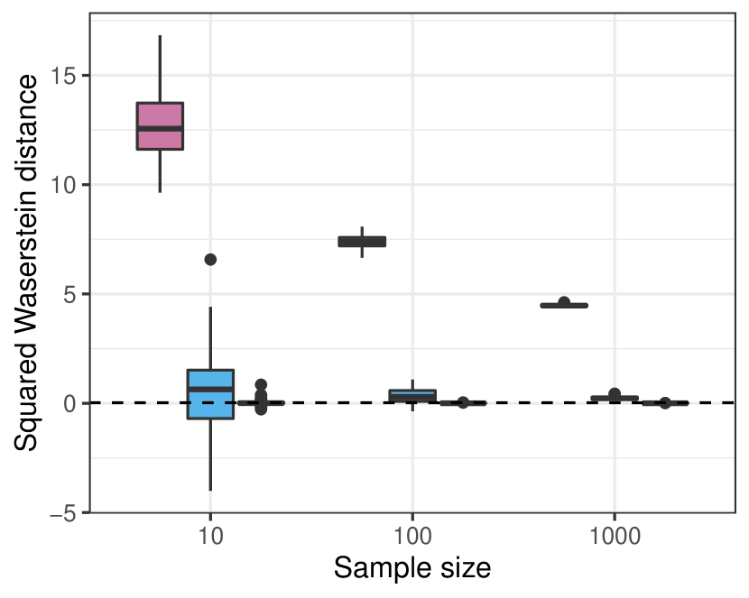
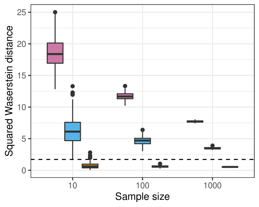
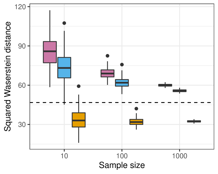
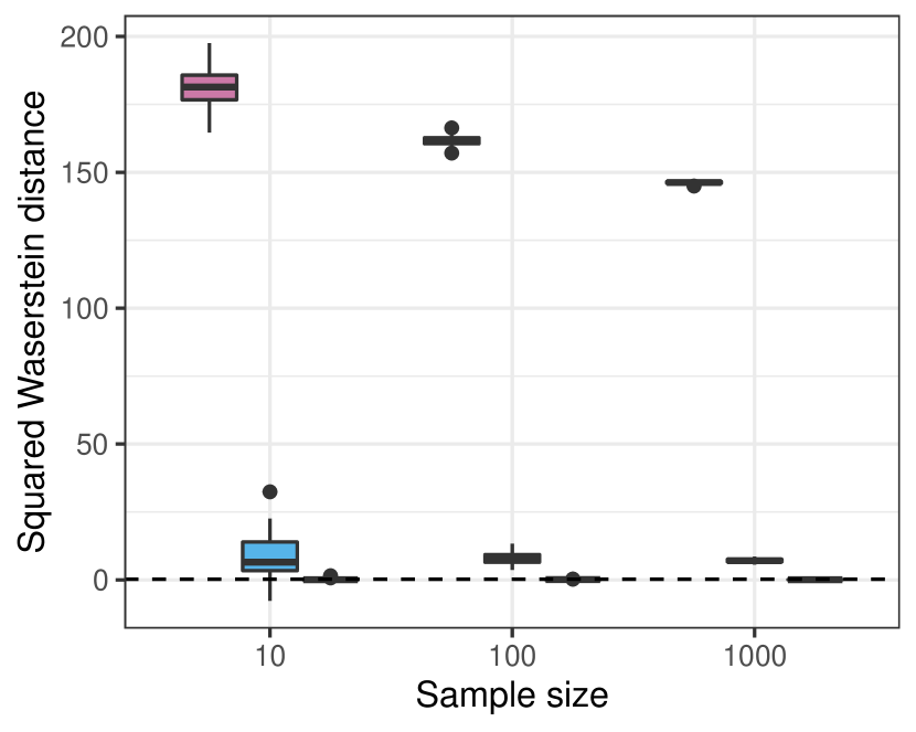
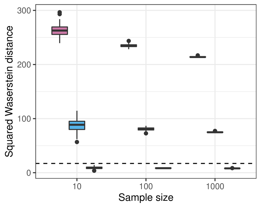
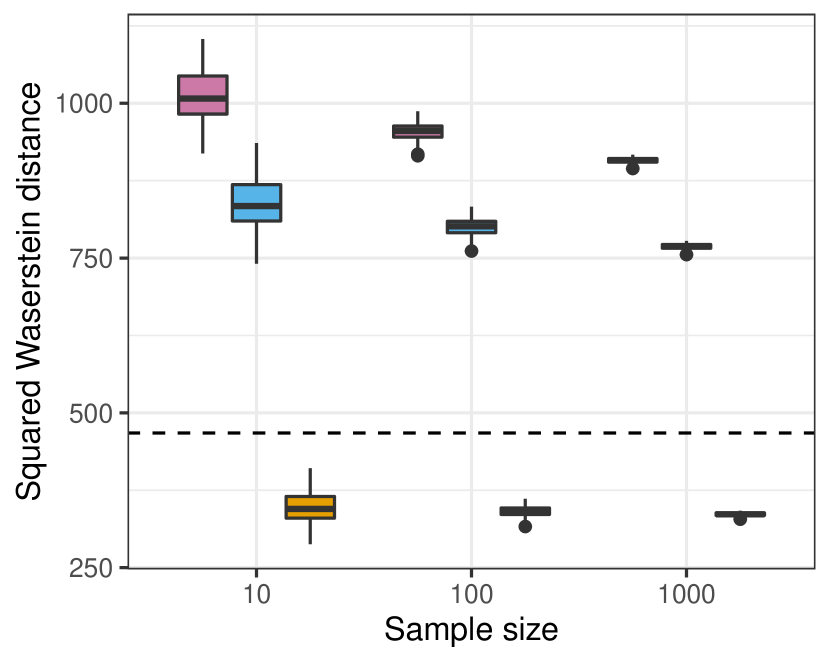
The results are presented in Figure 1. Relative to their biases, the noise in the estimators U𝑈U and Lsqsubscript𝐿sqL_{\textup{sq}} is under control at the higher sample sizes n𝑛n. Compared to the plug-in estimator 𝒲22(μ^n,ν^n)superscriptsubscript𝒲22subscript^𝜇𝑛subscript^𝜈𝑛\mathcal{W}_{2}^{2}(\hat{\mu}_{n},\hat{\nu}_{n}), the upper bound estimator U𝑈U has a greatly reduced absolute and relative error for the smaller values of σ2superscript𝜎2\sigma^{2}. The relative error of the estimator U𝑈U increases as σ2superscript𝜎2\sigma^{2} is decreased, as suggested by Proposition 1. As seen in Theorem 6, the rate of convergence of estimator U𝑈U suffers from the curse of dimensionality similarly to the plug-in estimator 𝒲22(μ^n,ν^n)superscriptsubscript𝒲22subscript^𝜇𝑛subscript^𝜈𝑛\mathcal{W}_{2}^{2}(\hat{\mu}_{n},\hat{\nu}_{n}).

The relative error of the estimator 𝔼Lsq𝔼subscript𝐿sq\mathbb{E}L_{\textup{sq}} increases as σ2superscript𝜎2\sigma^{2} decreases, at sample size n=1000𝑛1000n=1000 ranging between 0.140.140.14 and 0.690.690.69 in dimension d=10𝑑10d=10, and ranging between 0.370.370.37 and 0.710.710.71 in dimension d=100𝑑100d=100. As a bound for 𝒲22(μ^n,ν^n)superscriptsubscript𝒲22subscript^𝜇𝑛subscript^𝜈𝑛\mathcal{W}_{2}^{2}(\hat{\mu}_{n},\hat{\nu}_{n}), 𝔼Lsq𝔼subscript𝐿sq\mathbb{E}L_{\textup{sq}} appears to loosen slightly as n𝑛n is increased. This is due to the differing rates of convergence of the two terms in the estimator L𝐿L (recall that Lsq=sign(L)L2subscript𝐿sqsign𝐿superscript𝐿2L_{\textup{sq}}=\operatorname{sign}(L)L^{2}), where the first term 𝒲2(μ^n,ν^n)subscript𝒲2subscript^𝜇𝑛subscript^𝜈𝑛\mathcal{W}_{2}(\hat{\mu}_{n},\hat{\nu}_{n}) converges to 𝒲2(μ,ν)subscript𝒲2𝜇𝜈\mathcal{W}_{2}(\mu,\nu) at rate n2/dsuperscript𝑛2𝑑n^{-2/d}, while the second term 𝒲2(μ^n,μ^n)subscript𝒲2subscript^𝜇𝑛superscriptsubscript^𝜇𝑛\mathcal{W}_{2}(\hat{\mu}_{n},\hat{\mu}_{n}^{\prime}) converges to zero at a slower rate n1/dsuperscript𝑛1𝑑n^{-1/d}. For large enough n𝑛n, the average 𝔼Lsq𝔼subscript𝐿sq\mathbb{E}L_{\textup{sq}} does however converge from below to 𝒲22(μ,ν)superscriptsubscript𝒲22𝜇𝜈\mathcal{W}_{2}^{2}(\mu,\nu).

Refer to caption
Refer to caption
Refer to caption
Refer to caption
Refer to caption
Refer to caption
Figure 1: Box plots for 100 of each estimator (left to right for each sample size) 𝒲22(μ^n,ν^n)superscriptsubscript𝒲22subscript^𝜇𝑛subscript^𝜈𝑛\mathcal{W}_{2}^{2}(\hat{\mu}_{n},\hat{\nu}_{n}) ( ), U(ν^n,μ^n,μ^n)𝑈subscript^𝜈𝑛subscript^𝜇𝑛superscriptsubscript^𝜇𝑛U(\hat{\nu}_{n},\hat{\mu}_{n},\hat{\mu}_{n}^{\prime}) ( ) and Lsq(ν^n,μ^n,μ^n)subscript𝐿sqsubscript^𝜈𝑛subscript^𝜇𝑛superscriptsubscript^𝜇𝑛L_{\textup{sq}}(\hat{\nu}_{n},\hat{\mu}_{n},\hat{\mu}_{n}^{\prime}) ( ), compared with 𝒲22(μ,ν)superscriptsubscript𝒲22𝜇𝜈\mathcal{W}_{2}^{2}(\mu,\nu) ( ). Distributions μ=𝒩d(0,Id)𝜇subscript𝒩𝑑0subscript𝐼𝑑\mu=\mathcal{N}_{d}(0,I_{d}) and ν=𝒩d(0,σ2Id)𝜈subscript𝒩𝑑0superscript𝜎2subscript𝐼𝑑\nu=\mathcal{N}_{d}(0,\sigma^{2}I_{d}) were compared. The sample size n{10,100,1000}𝑛101001000n\in\{10,100,1000\}, the rows correspond to d{10,100}𝑑10100d\in\{10,100\} and the columns correspond to σ2{1.1,2,10}superscript𝜎21.1210\sigma^{2}\in\{1.1,2,10\}.

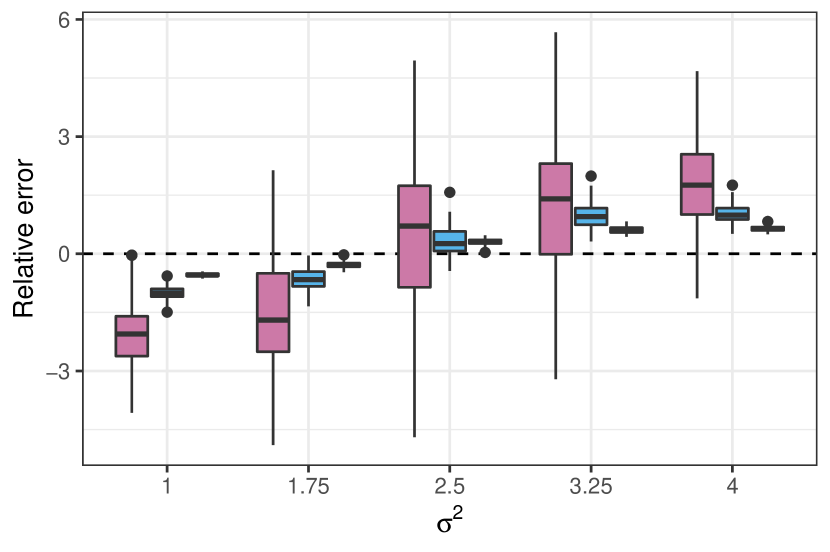
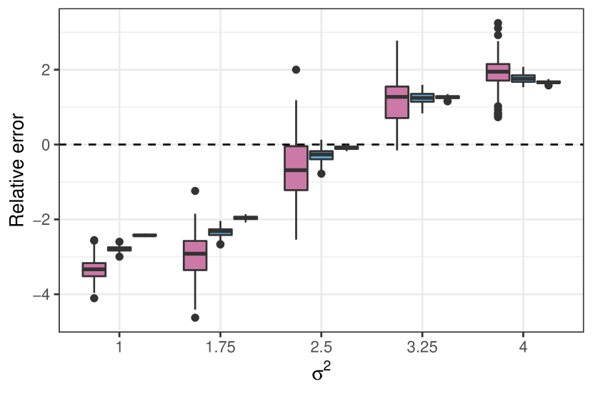
Secondly, we investigate how necessary the overdispersion condition νcotμ𝜈cot𝜇\nu\smash{\overset{\vphantom{a}\smash{\textup{cot}}}{\rightsquigarrow}}\mu is for the upper bound of Theorem 1. For this, we plot the relative error of the estimator U(ν^n,μ^n,μ^n)𝒲22(μ,ν)𝑈subscript^𝜈𝑛subscript^𝜇𝑛superscriptsubscript^𝜇𝑛superscriptsubscript𝒲22𝜇𝜈U(\hat{\nu}_{n},\hat{\mu}_{n},\hat{\mu}_{n}^{\prime})-\mathcal{W}_{2}^{2}(\mu,\nu), where μ=𝒩d(0,diag(1,4,1,4,))𝜇subscript𝒩𝑑0diag1414\mu=\mathcal{N}_{d}(0,\textup{diag}(1,4,1,4,\dots)), ν=𝒩d(0,σ2Id)𝜈subscript𝒩𝑑0superscript𝜎2subscript𝐼𝑑\nu=\mathcal{N}_{d}(0,\sigma^{2}I_{d}), and the parameters vary according to (σ2,d,n){1,1.75,2.5,3.25,4}×{10,100}×{10,100,1000}.superscript𝜎2𝑑𝑛11.752.53.25410100101001000(\sigma^{2},d,n)\in\{1,1.75,2.5,3.25,4\}\times\{10,100\}\times\{10,100,1000\}. The range of σ2superscript𝜎2\sigma^{2} is chosen so that μcotν𝜇cot𝜈\mu\smash{\overset{\vphantom{a}\smash{\textup{cot}}}{\rightsquigarrow}}\nu at σ2=1superscript𝜎21\sigma^{2}=1 (so that 𝔼U𝔼𝑈\mathbb{E}U is a lower bound according to Theorem 1), and νcotμ𝜈cot𝜇\nu\smash{\overset{\vphantom{a}\smash{\textup{cot}}}{\rightsquigarrow}}\mu at σ2=4superscript𝜎24\sigma^{2}=4 (so that 𝔼U𝔼𝑈\mathbb{E}U is an upper bound according to Theorem 1). The results are shown in Figure 2, and suggest that overdispersion which is weaker than νcotμ𝜈cot𝜇\nu\smash{\overset{\vphantom{a}\smash{\textup{cot}}}{\rightsquigarrow}}\mu may suffice for the upper bound of Theorem 1 to hold. The breaking point appears to be around σ2=2.5superscript𝜎22.5\sigma^{2}=2.5, at which point the traces of the covariances of ν𝜈\nu and μ𝜇\mu are identical, and above which the sum of the second moments of all components of ν𝜈\nu is larger than the corresponding quantity for μ𝜇\mu.

Refer to caption
Refer to caption
Figure 2: Box plots for the relative error of U(ν^n,μ^n,μ^n)𝑈subscript^𝜈𝑛subscript^𝜇𝑛superscriptsubscript^𝜇𝑛U(\hat{\nu}_{n},\hat{\mu}_{n},\hat{\mu}_{n}^{\prime}) (100 replicates) as an estimator of 𝒲22(μ,ν)superscriptsubscript𝒲22𝜇𝜈\mathcal{W}_{2}^{2}(\mu,\nu), with dashed line at y=0𝑦0y=0. Distributions μ=𝒩d(0,diag(1,4,1,4,))𝜇subscript𝒩𝑑0diag1414\mu=\mathcal{N}_{d}(0,\textup{diag}(1,4,1,4,\dots)) and ν=𝒩d(0,σ2Id)𝜈subscript𝒩𝑑0superscript𝜎2subscript𝐼𝑑\nu=\mathcal{N}_{d}(0,\sigma^{2}I_{d}) were compared in dimension d=10𝑑10d=10 (left) and d=100𝑑100d=100 (right). Sample sizes were n=10𝑛10n=10 ( ), n=100𝑛100n=100 ( ), n=1000𝑛1000n=1000 ( ). Theorem 1 indicates a lower bound in expectation at the minimum of σ2=1superscript𝜎21\sigma^{2}=1, and an upper bound in expectation at the maximum of σ2=4superscript𝜎24\sigma^{2}=4.

3 Uncertainty quantification

Having removed a large part of the bias in the empirical estimator of the Wasserstein distance, noise becomes a larger issue, and so now we quantify the uncertainty in the point estimators of the bounds (1), (2). We first derive a central limit theorem, following results in delbarrio2019central; delbarrio2021central. This motivates Gaussian confidence intervals for the upper bound (1). Lacking satisfactory distributional results, we suggest using Chebyshev’s theorem to obtain conservative confidence intervals for the lower bound (2).

Both types of confidence intervals rely on estimating the variance of the point estimators. We suggest doing so conservatively by the jackknife method (efron1981the), and we propose the Flapjack algorithm to compute the leave-one-out jackknife estimates efficiently.

3.1 Central limit theorems and confidence intervals

We shall impose the following regularity conditions, borrowed from delbarrio2021central.

Assumption 3 (Regularity and bounded fourth moments).

μ,ν𝒫(d)𝜇𝜈𝒫superscript𝑑\mu,\nu\in\mathcal{P}(\mathbb{R}^{d}) are continuous, have connected supports with negligible boundary, and have finite moments of order 4+δ4𝛿4+\delta for some δ>0𝛿0\delta>0, that is 𝔼μX4+δsubscript𝔼𝜇superscriptdelimited-∥∥𝑋4𝛿\mathbb{E}_{\mu}\lVert X\rVert^{4+\delta}\leq\infty and 𝔼νY4+δsubscript𝔼𝜈superscriptdelimited-∥∥𝑌4𝛿\mathbb{E}_{\nu}\lVert Y\rVert^{4+\delta}\leq\infty.

Under these conditions, a Gaussian central limit theorem holds for the estimator U𝑈U. As noted by delbarrio2019central; delbarrio2021central, the limiting variance is null when μ=ν𝜇𝜈\mu=\nu (the Kantorovich potentials are constant). In this case, the theorem indicates that the variance of U𝑈U decreases strictly faster than the canonical rate n1superscript𝑛1n^{-1}. If a non-trivial limit of a similar type exists when μ=ν𝜇𝜈\mu=\nu, its leading factor must grow strictly faster then n1/2superscript𝑛12n^{1/2}. The existence and form of such theorems are open questions for both U𝑈U and the plug-in estimator 𝒲22(μ^n,μ^n)superscriptsubscript𝒲22subscript^𝜇𝑛subscriptsuperscript^𝜇𝑛\mathcal{W}_{2}^{2}(\hat{\mu}_{n},\hat{\mu}^{\prime}_{n}).

Theorem 7 (Central limit theorem for the upper bound estimator).

Under Assumptions 1 and 3, it holds that

n1/2(U𝔼U)superscript𝑛12𝑈𝔼𝑈\displaystyle n^{1/2}(U-\mathbb{E}U) 𝒩(0,σ2),absent𝒩0superscript𝜎2\displaystyle\implies\mathcal{N}(0,\sigma^{2}),
limnnVarUsubscript𝑛𝑛Var𝑈\displaystyle\lim_{n\to\infty}n\operatorname{Var}U =σ2.absentsuperscript𝜎2\displaystyle=\sigma^{2}.

σ2=Varμφ(X)+Varνψ(Y)superscript𝜎2subscriptVar𝜇𝜑𝑋subscriptVar𝜈𝜓𝑌\sigma^{2}=\operatorname{Var}_{\mu}\varphi(X)+\operatorname{Var}_{\nu}\psi(Y), and (φ,ψ)𝜑𝜓(\varphi,\psi) are the Kantorovich potentials (see Appendix A) when transporting μ𝜇\mu to ν𝜈\nu.

Theorem 7 motivates the usage of the usual Gaussian asymptotic confidence intervals for 𝔼U𝔼𝑈\mathbb{E}U when μν𝜇𝜈\mu\neq\nu. Given an estimate σ^2superscript^𝜎2\hat{\sigma}^{2} of the variance of U𝑈U, a (1α)1𝛼(1-\alpha)-level confidence interval is [Uσ^zα/2,U+σ^z1α/2]𝑈^𝜎subscript𝑧𝛼2𝑈^𝜎subscript𝑧1𝛼2[U-\hat{\sigma}z_{\alpha/2},U+\hat{\sigma}z_{1-\alpha/2}]. The coverage is asymptotically exact if the variance estimate σ^2superscript^𝜎2\hat{\sigma}^{2} is exact. When μ=ν𝜇𝜈\mu=\nu, the asymptotic theory is lacking, and therefore such confidence intervals are currently out of reach (however note that the distribution of U𝑈U is symmetric about the origin). Chebyshev’s inequality could then be used to construct conservative confidence intervals for U𝑈U, as we outline for the estimator L𝐿L below.

When μν𝜇𝜈\mu\neq\nu, following the proof of Theorem 4.9 in delbarrio2021central together with a simple observation, one can derive a non-trivial limit for 𝒲2(ν^n,μ^n)subscript𝒲2subscript^𝜈𝑛subscript^𝜇𝑛\mathcal{W}_{2}(\hat{\nu}_{n},\hat{\mu}_{n}) which is centered around its mean 𝔼𝒲2(ν^n,μ^n)𝔼subscript𝒲2subscript^𝜈𝑛subscript^𝜇𝑛\mathbb{E}\mathcal{W}_{2}(\hat{\nu}_{n},\hat{\mu}_{n}) (see Appendix B.4). The method does not extend to obtain a centered limit for 𝒲2(μ^n,μ^n)subscript𝒲2subscriptsuperscript^𝜇𝑛subscript^𝜇𝑛\mathcal{W}_{2}(\hat{\mu}^{\prime}_{n},\hat{\mu}_{n}). As such, we have not been able to derive satisfactory central limits for the lower bound estimator L𝐿L. In order to estimate conservative confidence intervals for L𝐿L, we instead suggest using Chebyshev’s inequality. If τ^2superscript^𝜏2\hat{\tau}^{2} is an estimate of the variance of L𝐿L, then a confidence interval with more than (1α)1𝛼(1-\alpha) coverage is [Lτ^α1/2,L+τ^α1/2]𝐿^𝜏superscript𝛼12𝐿^𝜏superscript𝛼12[L-\hat{\tau}\alpha^{-1/2},L+\hat{\tau}\alpha^{-1/2}]. Compared to a Gaussian 95%percent9595\% confidence interval, a Chebyshev confidence interval is approximately 2.3 times wider.

3.2 Jackknife variance estimation

An estimate of the variance of a statistic F(X1,,Xn)𝐹subscript𝑋1subscript𝑋𝑛F(X_{1},\dots,X_{n}) can be obtained via the jackknife method (efron1981the). This proceeds by first computing the leave-one-out statistics Fi=F(X1,,Xi1,Xi+1,,Xn)subscript𝐹𝑖𝐹subscript𝑋1subscript𝑋𝑖1subscript𝑋𝑖1subscript𝑋𝑛F_{i}=F(X_{1},\dots,X_{i-1},X_{i+1},\dots,X_{n}) for i=1,,n𝑖1𝑛i=1,\dots,n. Then, one combines these into the jackknife variance estimate

n1ni=1n(Fi1ni=1nFi)2.𝑛1𝑛superscriptsubscript𝑖1𝑛superscriptsubscript𝐹𝑖1𝑛superscriptsubscript𝑖1𝑛subscript𝐹𝑖2\frac{n-1}{n}\sum_{i=1}^{n}\big{(}F_{i}-\frac{1}{n}\sum_{i=1}^{n}F_{i}\big{)}^{2}.

The first term is a sample size correction, and the second term is a positively biased estimate of the sample size n1𝑛1n-1 variance, as per the Efron-Stein inequality (efron1981the).

3.2.1 The Flapjack algorithm

At sample size n𝑛n, an empirical transportation cost (including the squared empirical Wasserstein distance) is computed via a linear assignment problem of the following form,

T=minx𝑇subscript𝑥\displaystyle T=\min_{x} i,j=1ncijxij,superscriptsubscript𝑖𝑗1𝑛subscript𝑐𝑖𝑗subscript𝑥𝑖𝑗\displaystyle\sum_{i,j=1}^{n}c_{ij}x_{ij}, (3)
s.t. k=1nxik=1/n,k=1nxkj=1/n,xij0,i,j=1,,n.formulae-sequencesuperscriptsubscript𝑘1𝑛subscript𝑥𝑖𝑘1𝑛formulae-sequencesuperscriptsubscript𝑘1𝑛subscript𝑥𝑘𝑗1𝑛formulae-sequencesubscript𝑥𝑖𝑗0for-all𝑖𝑗1𝑛\displaystyle\sum_{k=1}^{n}x_{ik}=1/n,\quad\sum_{k=1}^{n}x_{kj}=1/n,\quad x_{ij}\geq 0,\quad\forall i,j=1,\dots,n.

This is equivalent to the Kantorovich formulation of the optimal transportation problem. At the optimum, all xijsubscript𝑥𝑖𝑗x_{ij} are either 00 or 1/n1𝑛1/n, such that there exists an optimal assignment (or matching) σ𝒮n𝜎subscript𝒮𝑛\sigma\in\mathcal{S}_{n} with the property that i,j{1,,n}𝑖𝑗1𝑛i,j\in\{1,\dots,n\}, xij=1/nsubscript𝑥𝑖𝑗1𝑛x_{ij}=1/n if and only if j=σ(i)𝑗𝜎𝑖j=\sigma(i). This primal assignment problem admits the following dual formulation

maxu,vsubscript𝑢𝑣\displaystyle\max_{u,v}\quad 1ni=1nui+1nj=1nvj,1𝑛superscriptsubscript𝑖1𝑛subscript𝑢𝑖1𝑛superscriptsubscript𝑗1𝑛subscript𝑣𝑗\displaystyle\frac{1}{n}\sum_{i=1}^{n}u_{i}+\frac{1}{n}\sum_{j=1}^{n}v_{j},
s.t. ui+vjciji,j=1,,n.formulae-sequencesubscript𝑢𝑖subscript𝑣𝑗subscript𝑐𝑖𝑗for-all𝑖𝑗1𝑛\displaystyle u_{i}+v_{j}\leq c_{ij}\quad\forall i,j=1,\dots,n.

To compute the jackknife variance estimate of the solution, one needs to first solve the n𝑛n leave-one-out problems (3) at sample size n1𝑛1n-1. Since the exact computation of the sample size n𝑛n problem takes O(n3)𝑂superscript𝑛3O(n^{3}) time, naively computing the jackknife variance estimate would require a prohibitive O(n4)𝑂superscript𝑛4O(n^{4}) time.

Starting from a joint solution of the sample size n𝑛n primal and dual problems, it is however possible to compute the jackknife variance estimate of the cost in O(n3)𝑂superscript𝑛3O(n^{3}) time, no worse than the complexity of solving the original optimization problem. As proven in mills-tettey2007the, if only a single entry, row, or column of the cost matrix (cij)subscript𝑐𝑖𝑗(c_{ij}) changes, then the Hungarian algorithm can be employed to solve the modified problem in O(n2)𝑂superscript𝑛2O(n^{2}) time. This motivates the Flapjack algorithm (for Fast Linear Assignment Problem with JACKknife estimates), which repairs the sample size n𝑛n optimal solution to solve the n𝑛n sample size n1𝑛1n-1 sub-problems in O(n2)𝑂superscript𝑛2O(n^{2}) time each. To compute the i𝑖i-th leave-one-out estimate, we first change the cost ciisubscript𝑐𝑖𝑖c_{ii} to a small enough value, which forces xii=1/nsubscript𝑥𝑖𝑖1𝑛x_{ii}=1/n at the optimum, and then simply drop ciixiisubscript𝑐𝑖𝑖subscript𝑥𝑖𝑖c_{ii}x_{ii} from the final objective value. The Flapjack algorithm is provided in Appendix E.1 as Algorithm 1.

3.3 Numerical illustration

In this section, we illustrate the behaviour of the jackknife variance estimator for U(ν^n,μ^n,μ^n)𝑈subscript^𝜈𝑛subscript^𝜇𝑛superscriptsubscript^𝜇𝑛U(\hat{\nu}_{n},\hat{\mu}_{n},\hat{\mu}_{n}^{\prime}) when μ=𝒩d(0,Id)𝜇subscript𝒩𝑑0subscript𝐼𝑑\mu=\mathcal{N}_{d}(0,I_{d}) and ν=𝒩d(0,σ2Id)𝜈subscript𝒩𝑑0superscript𝜎2subscript𝐼𝑑\nu=\mathcal{N}_{d}(0,\sigma^{2}I_{d}) and the parameters vary according to (σ2,d,n){1.1,10}×{10,100}×{10,100,1000}.superscript𝜎2𝑑𝑛1.11010100101001000(\sigma^{2},d,n)\in\{1.1,10\}\times\{10,100\}\times\{10,100,1000\}.

To simplify the presentation, and as the results are similar, we show no results for the plug-in estimator 𝒲22(μ^n,ν^n)superscriptsubscript𝒲22subscript^𝜇𝑛subscript^𝜈𝑛\mathcal{W}_{2}^{2}(\hat{\mu}_{n},\hat{\nu}_{n}) or the lower bound estimator L(ν^n,μ^n,μ^n)𝐿subscript^𝜈𝑛subscript^𝜇𝑛superscriptsubscript^𝜇𝑛L(\hat{\nu}_{n},\hat{\mu}_{n},\hat{\mu}_{n}^{\prime}). The jackknife variance estimates are compared with the variance of U𝑈U in Figure 3. The jackknife variance estimates are conservative, and at worst are, in expectation, approximately a factor of 222 larger than the true variance. As σ2superscript𝜎2\sigma^{2} decreases, the jackknife estimates become progressively more conservative. We also find that 95%percent9595\%-level jackknife confidence intervals for the estimator U𝑈U, derived from the Gaussian limit of Theorem 7, have at least the nominal coverage for sample sizes n100𝑛100n\geq 100.

Refer to caption
Refer to caption
Refer to caption
Refer to caption
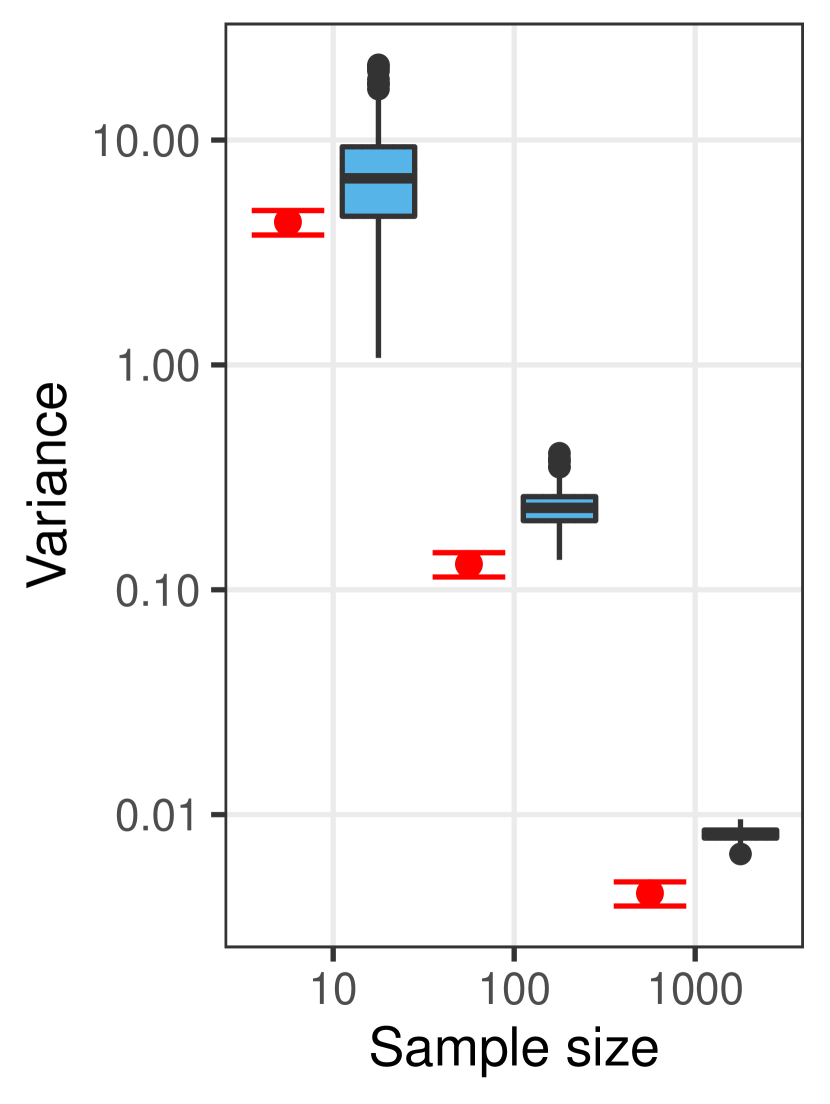
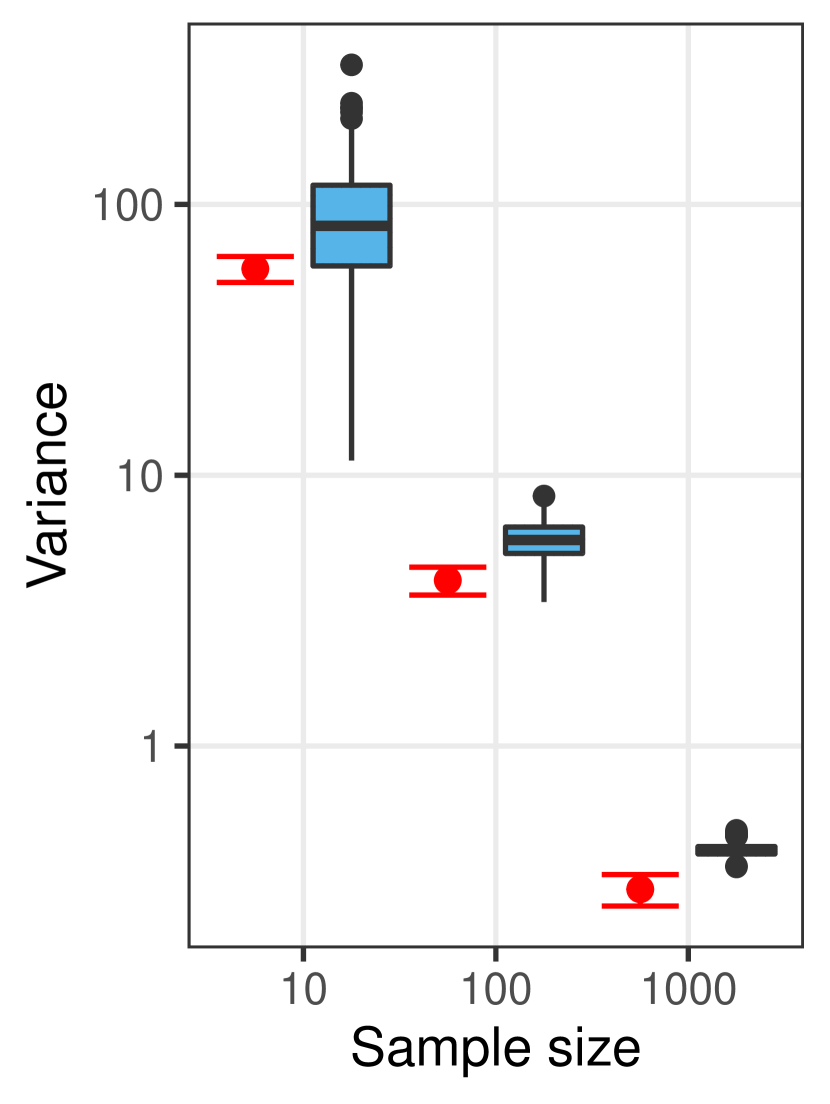
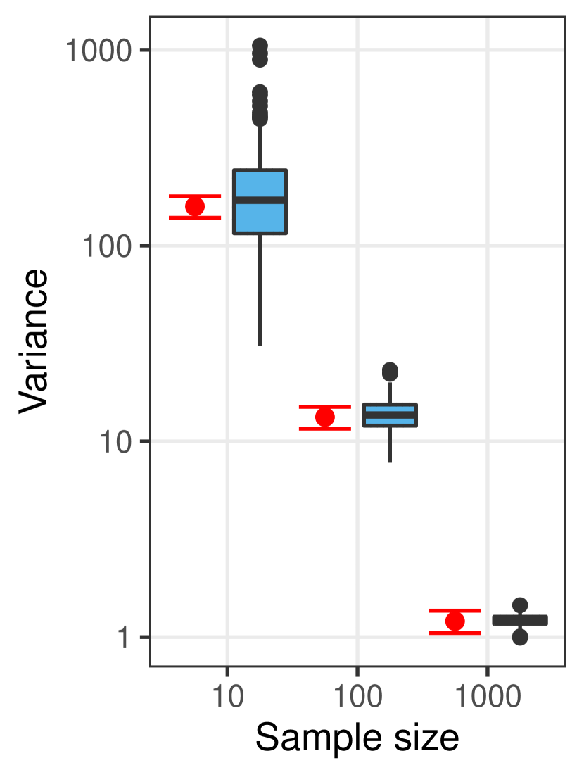
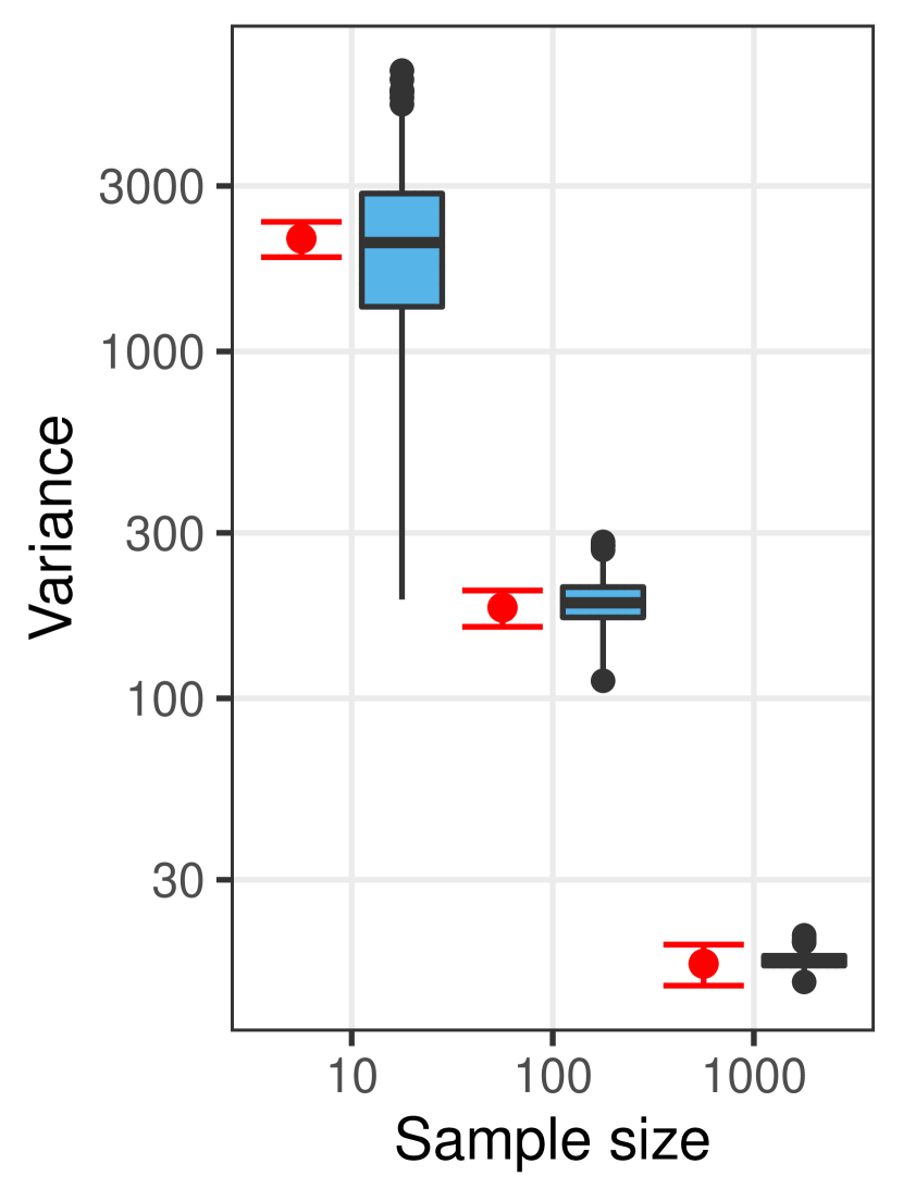
Figure 3: Box plots of jackknife variance estimates for U(ν^n,μ^n,μ^n)𝑈subscript^𝜈𝑛subscript^𝜇𝑛superscriptsubscript^𝜇𝑛U(\hat{\nu}_{n},\hat{\mu}_{n},\hat{\mu}_{n}^{\prime}) ( ); empirical variance with bootstrap 95%percent9595\% confidence intervals ( ). Distributions μ=𝒩d(0,Id)𝜇subscript𝒩𝑑0subscript𝐼𝑑\mu=\mathcal{N}_{d}(0,I_{d}) and ν=𝒩d(0,σ2Id)𝜈subscript𝒩𝑑0superscript𝜎2subscript𝐼𝑑\nu=\mathcal{N}_{d}(0,\sigma^{2}I_{d}) were compared with, left to right, (d,σ2){(10,1.1),(100,1.1),(10,10),(100,10)}𝑑superscript𝜎2101.11001.1101010010(d,\sigma^{2})\in\{(10,1.1),(100,1.1),(10,10),(100,10)\}. For each sample size n{10,100,1000}𝑛101001000n\in\{10,100,1000\}, 500 replicates of the estimator and its jackknife variance estimator were computed. These 500 replicates were used to compute the empirical variance. Confidence intervals for the empirical variance were computed with 500 bootstrap samples.

4 Bounding the Wasserstein distance in MCMC

Let (Xt)t0subscriptsubscript𝑋𝑡𝑡0(X_{t})_{t\geq 0} represent an MCMC Markov chain where the time-t𝑡t marginals, πtsubscript𝜋𝑡\pi_{t}, and the stationary distribution, πsubscript𝜋\pi_{\infty}, are all continuous and have finite second moments. Multiple independent copies of the chain are run generating empirical measures π^tsubscript^𝜋𝑡\hat{\pi}_{t} for t0𝑡0t\geq 0; with the same number of samples each, the two empirical measures π^,π^subscript^𝜋superscriptsubscript^𝜋\hat{\pi}_{\infty},\hat{\pi}_{\infty}^{\prime} are drawn independently from the stationary distribution.

As long as the chain remains overdispersed with respect to its stationary distribution for all iterations t0𝑡0t\geq 0, our empirical bounds can be applied to quantify the convergence of the Markov chain. In the following corollary, the first inequality restates Proposition 1, the second restates Theorem 1, and the third restates Theorem 2.

Corollary 2 (Bounds for MCMC).

Let K𝐾K be as in Proposition 1. If πtcotπsubscript𝜋𝑡cotsubscript𝜋\pi_{t}\overset{\vphantom{a}\smash{\textup{cot}}}{\rightsquigarrow}\pi_{\infty}, then

K(πt,π)𝒲2(πt,π)𝐾subscript𝜋𝑡subscript𝜋subscript𝒲2subscript𝜋𝑡subscript𝜋\displaystyle K(\pi_{t},\pi_{\infty})\mathcal{W}_{2}(\pi_{t},\pi_{\infty}) 𝔼[𝒲22(π^t,π^)𝒲22(π^,π^)]𝒲22(πt,π).absent𝔼delimited-[]superscriptsubscript𝒲22subscript^𝜋𝑡subscript^𝜋superscriptsubscript𝒲22subscriptsuperscript^𝜋subscript^𝜋superscriptsubscript𝒲22subscript𝜋𝑡subscript𝜋\displaystyle\geq\;\mathbb{E}\left[\mathcal{W}_{2}^{2}(\hat{\pi}_{t},\hat{\pi}_{\infty})-\mathcal{W}_{2}^{2}(\hat{\pi}^{\prime}_{\infty},\hat{\pi}_{\infty})\right]\geq\mathcal{W}_{2}^{2}(\pi_{t},\pi_{\infty}).
𝒲2(πt,π)subscript𝒲2subscript𝜋𝑡subscript𝜋\displaystyle\mathcal{W}_{2}(\pi_{t},\pi_{\infty}) |𝔼[𝒲2(π^t,π^)𝒲2(π^,π^)]|.absent𝔼delimited-[]subscript𝒲2subscript^𝜋𝑡subscript^𝜋subscript𝒲2subscriptsuperscript^𝜋subscript^𝜋\displaystyle\geq\left|\mathbb{E}\left[\mathcal{W}_{2}(\hat{\pi}_{t},\hat{\pi}_{\infty})-\mathcal{W}_{2}(\hat{\pi}^{\prime}_{\infty},\hat{\pi}_{\infty})\right]\right|.

In practice, independent samples from πsubscript𝜋\pi_{\infty} will not be available directly. However, we may estimate π^π^Tsubscript^𝜋subscript^𝜋𝑇\hat{\pi}_{\infty}\approx\hat{\pi}_{T} and π^π^Tsubscriptsuperscript^𝜋subscript^𝜋superscript𝑇\hat{\pi}^{\prime}_{\infty}\approx\hat{\pi}_{T^{\prime}} for some large for some large T<Tsuperscript𝑇𝑇T^{\prime}<T, chosen such that XTsubscript𝑋𝑇X_{T} and XTsubscript𝑋superscript𝑇X_{T^{\prime}} are approximately independent. In other words, we declare a priori that the chain has converged by time Tsuperscript𝑇T^{\prime}, and run it until a further iteration T𝑇T which produces samples approximately independently from iteration Tsuperscript𝑇T^{\prime}. The upper bound is useful to assess when before Tsuperscript𝑇T^{\prime} the chain has reached the stationary distribution, and how it has done so.

4.1 Persistence of overdispersion in MCMC

In practice, one is unlikely to be able to verify the condition πtcotπsubscript𝜋𝑡cotsubscript𝜋\pi_{t}\smash{\overset{\vphantom{a}\smash{\textup{cot}}}{\rightsquigarrow}}\pi_{\infty} for all t0𝑡0t\geq 0, whether analytically or numerically. However, if one starts off a Markov chain from π0cotπsubscript𝜋0cotsubscript𝜋\pi_{0}\smash{\overset{\vphantom{a}\smash{\textup{cot}}}{\rightsquigarrow}}\pi_{\infty}, then one may hope that, throughout its lifetime, the Markov chain does remain overdispersed with respect to its target, or at least approximately so. This subsection is concerned with checking whether this heuristic is reasonable, and when it might fail. We begin with analytically tractable Gaussian scenarios, where the answer is affirmative, and follow up with simulations in scenarios which are numerically tractable.

4.1.1 Analytically tractable scenarios

ULA and Gibbs chains which have Gaussian stationary and starting distributions also have analytically tractable Gaussian marginals. As per Proposition 2, we can therefore verify whether the overdispersion propagates throughout the marginals πtsubscript𝜋𝑡\pi_{t}, t0𝑡0t\geq 0. We find that this is indeed the case. However, caution is required: not starting the chains suitably overdispersed also ensures that πtsubscript𝜋𝑡\pi_{t} is never overdispersed with respect to πsubscript𝜋\pi_{\infty}.

Theorem 8 (cotcot\smash{\overset{\vphantom{a}\smash{\textup{cot}}}{\rightsquigarrow}} for chains with Gaussian marginals).

Suppose that πtsubscript𝜋𝑡\pi_{t} is the Gaussian marginal distribution at time t0𝑡0t\geq 0 of a Markov chain converging to a Gaussian stationary distribution πsubscript𝜋\pi_{\infty}. If the algorithm is (i)𝑖(i) a deterministically updating Gibbs sampler, or (ii)𝑖𝑖(ii) an unadjusted Langevin algorithm, then

π0cotππtcotπfor all t0.iffsubscript𝜋0cotsubscript𝜋subscript𝜋𝑡cotsubscript𝜋for all 𝑡0\pi_{0}\overset{\vphantom{a}\smash{\textup{cot}}}{\rightsquigarrow}\pi_{\infty}\iff\pi_{t}\overset{\vphantom{a}\smash{\textup{cot}}}{\rightsquigarrow}\pi_{\infty}\quad\text{for all }t\geq 0.

The Gibbs sampler need not update its coordinates one-at-a-time, as the result remains applicable for blocked Gibbs samplers as well.

4.1.2 Numerically tractable scenarios

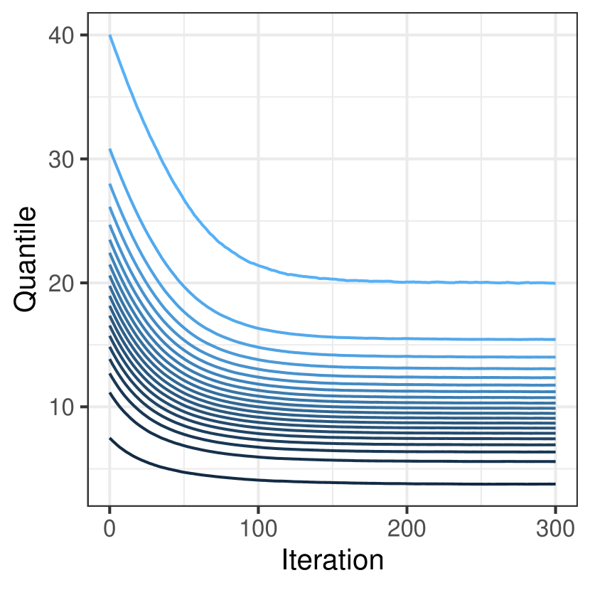
Following Section 2.2, in dimension d=1𝑑1d=1 one can check the condition πtcotπsubscript𝜋𝑡cot𝜋\pi_{t}\smash{\overset{\vphantom{a}\smash{\textup{cot}}}{\rightsquigarrow}}\pi by looking at the relative separation of the quantiles of these distributions. Similarly, in general dimension d𝑑d, for samplers whose target π𝜋\pi and time-t𝑡t marginals πtsubscript𝜋𝑡\pi_{t} are isotropic distributions, checking the condition πtcotπsubscript𝜋𝑡cot𝜋\pi_{t}\smash{\overset{\vphantom{a}\smash{\textup{cot}}}{\rightsquigarrow}}\pi simplifies to checking that the same relationship holds between the radial components of these distributions. Samplers that are appropriately isotropic include the random walk Metropolis (RWM) algorithm and the Metropolis-Adjusted Langevin Algorithm (MALA) using proposals with isotropic Gaussian noise.

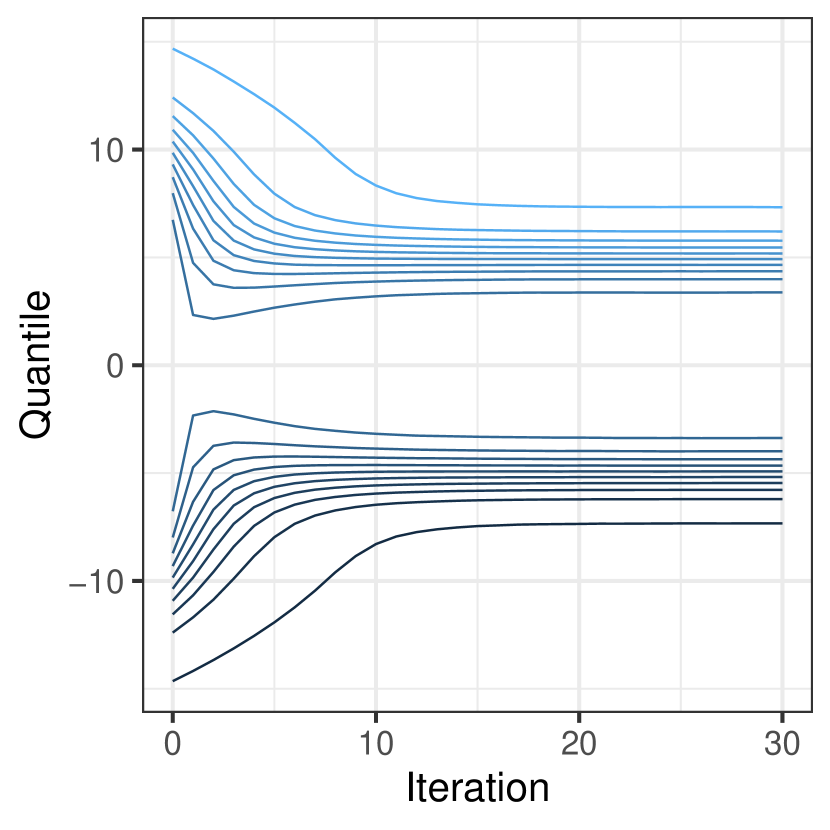
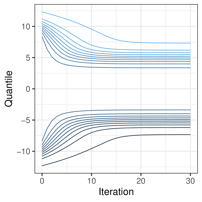
For the unimodal isotropic scenarios we investigated, π0cotπsubscript𝜋0cotsubscript𝜋\pi_{0}\smash{\overset{\vphantom{a}\smash{\textup{cot}}}{\rightsquigarrow}}\pi_{\infty} caused πtcotπsubscript𝜋𝑡cotsubscript𝜋\pi_{t}\smash{\overset{\vphantom{a}\smash{\textup{cot}}}{\rightsquigarrow}}\pi_{\infty} for all t0𝑡0t\geq 0. These examples correspond to diffusive MCMC samplers targeting unimodal distributions, whose starting distributions are spread-out with respect to the target in all directions. However, we found that multimodal targets can cause πtcotπsubscript𝜋𝑡cotsubscript𝜋\pi_{t}\smash{\overset{\vphantom{a}\smash{\textup{cot}}}{\rightsquigarrow}}\pi_{\infty} to not hold for arbitrary t>0𝑡0t>0, in spite of π0cotπsubscript𝜋0cot𝜋\pi_{0}\smash{\overset{\vphantom{a}\smash{\textup{cot}}}{\rightsquigarrow}}\pi holding. For the RWM algorithm targeting π=0.5𝒩1(5,1)+0.5𝒩1(5,1)𝜋0.5subscript𝒩1510.5subscript𝒩151\pi=0.5\mathcal{N}_{1}(-5,1)+0.5\mathcal{N}_{1}(5,1), a mixture distribution with well-separated modes, starting from π0=0.5𝒩1(10,4)+0.5𝒩1(10,4)cotπsubscript𝜋00.5subscript𝒩11040.5subscript𝒩1104cot𝜋\pi_{0}=0.5\mathcal{N}_{1}(-10,4)+0.5\mathcal{N}_{1}(10,4)\smash{\overset{\vphantom{a}\smash{\textup{cot}}}{\rightsquigarrow}}\pi and using a step size h=22h=2 (an acceptance rate of 50%percent5050\%), a single RWM chain seldom jumps between the modes, and πtcotπsubscript𝜋𝑡cotsubscript𝜋\pi_{t}\smash{\overset{\vphantom{a}\smash{\textup{cot}}}{\rightsquigarrow}}\pi_{\infty} holds for all t0𝑡0t\geq 0. Increasing the step size to h=66h=6 (an acceptance rate of 26%percent2626\%), a single RWM chain jumps between the modes more frequently, causing πtcotπsubscript𝜋𝑡cotsubscript𝜋\pi_{t}\smash{\overset{\vphantom{a}\smash{\textup{cot}}}{\rightsquigarrow}}\pi_{\infty} to fail for iterations t1𝑡1t\geq 1. For the start π0=0.5𝒩1(0,1)+0.5𝒩1(10,1)subscript𝜋00.5subscript𝒩1010.5subscript𝒩1101\pi_{0}=0.5\mathcal{N}_{1}(0,1)+0.5\mathcal{N}_{1}(10,1), a shifted version of πsubscript𝜋\pi_{\infty}, and h=22h=2, the majority of the chains initially jump to one mode, causing πtcotπsubscript𝜋𝑡cotsubscript𝜋\pi_{t}\smash{\overset{\vphantom{a}\smash{\textup{cot}}}{\rightsquigarrow}}\pi_{\infty} to again fail for t1𝑡1t\geq 1. Figure 4, and Figure 9 in Appendix E.2 display the previously outlined results.

These examples highlight the potential challenges posed to our method by multimodality, while offering reassurance that πtcotπsubscript𝜋𝑡cotsubscript𝜋\pi_{t}\smash{\overset{\vphantom{a}\smash{\textup{cot}}}{\rightsquigarrow}}\pi_{\infty} for t0𝑡0t\geq 0 can hold for diffusive MCMC samplers started at π0cotπsubscript𝜋0cotsubscript𝜋\pi_{0}\smash{\overset{\vphantom{a}\smash{\textup{cot}}}{\rightsquigarrow}}\pi_{\infty} and targeting unimodal distributions.
Refer to caption
Refer to caption
Refer to caption
Figure 4: Quantiles of the radial component of πtsubscript𝜋𝑡\pi_{t} (left) and πtsubscript𝜋𝑡\pi_{t} (middle, right) against iteration t0𝑡0t\geq 0, from probability 0.005 (dark blue) to 0.995 (light blue) for the RWM algorithm. Left: 10-dimensional logistic target π(x)exp(x)/{1+exp(x)}2proportional-to𝜋𝑥delimited-∥∥𝑥superscript1delimited-∥∥𝑥2\pi(x)\propto\exp(\lVert x\rVert)/\{1+\exp(\lVert x\rVert)\}^{2} with starting density π0(x)π(x/2)proportional-tosubscript𝜋0𝑥𝜋𝑥2\pi_{0}(x)\propto\pi(x/2). Middle and right: mixture target π=0.5𝒩1(5,1)+0.5𝒩1(5,1)𝜋0.5subscript𝒩1510.5subscript𝒩151\pi=0.5\mathcal{N}_{1}(-5,1)+0.5\mathcal{N}_{1}(5,1), with start π0=0.5𝒩1(10,4)+0.5𝒩1(10,4)subscript𝜋00.5subscript𝒩11040.5subscript𝒩1104\pi_{0}=0.5\mathcal{N}_{1}(-10,4)+0.5\mathcal{N}_{1}(10,4) and step sizes h=22h=2 (left) and h=66h=6 (right). The condition πtcotπsubscript𝜋𝑡cotsubscript𝜋\pi_{t}\smash{\overset{\vphantom{a}\smash{\textup{cot}}}{\rightsquigarrow}}\pi_{\infty} holds for all t0𝑡0t\geq 0 in the left and middle plots, but fails for t>0𝑡0t>0 in the right plot.

4.2 Confidence intervals in MCMC

Just as before in Section 3.1, we have a Gaussian central limit theorem for the upper bound estimator in MCMC. This follows from Proposition 3 (Appendix B).

Theorem 9 (CLT for MCMC setting).

Suppose that πt,πT,πTsubscript𝜋𝑡subscript𝜋𝑇subscript𝜋superscript𝑇\pi_{t},\pi_{T},\pi_{T^{\prime}} satisfy Assumption 3. Then,

n1/2(U(π^t,π^T,π^T)𝔼U(π^t,π^T,π^T))superscript𝑛12𝑈subscript^𝜋𝑡subscript^𝜋𝑇subscript^𝜋superscript𝑇𝔼𝑈subscript^𝜋𝑡subscript^𝜋𝑇subscript^𝜋superscript𝑇\displaystyle n^{1/2}\left(U(\hat{\pi}_{t},\hat{\pi}_{T},\hat{\pi}_{T^{\prime}})-\mathbb{E}U(\hat{\pi}_{t},\hat{\pi}_{T},\hat{\pi}_{T^{\prime}})\right) 𝒩(0,σ2),absent𝒩0superscript𝜎2\displaystyle\implies\mathcal{N}(0,\sigma^{2}),
limnnVarU(π^t,π^T,π^T)subscript𝑛𝑛Var𝑈subscript^𝜋𝑡subscript^𝜋𝑇subscript^𝜋superscript𝑇\displaystyle\lim_{n\to\infty}n\operatorname{Var}U(\hat{\pi}_{t},\hat{\pi}_{T},\hat{\pi}_{T^{\prime}}) =σ2.absentsuperscript𝜎2\displaystyle=\sigma^{2}.

The limiting variance is σ2=Var{φtT(Xt)+φTt(XT)+φTT(XT)+φTT(XT)}superscript𝜎2Varsubscript𝜑𝑡𝑇subscript𝑋𝑡subscript𝜑𝑇𝑡subscript𝑋𝑇subscript𝜑𝑇superscript𝑇subscript𝑋𝑇subscript𝜑superscript𝑇𝑇subscript𝑋superscript𝑇\sigma^{2}=\operatorname{Var}\{\varphi_{t\to T}(X_{t})+\varphi_{T\to t}(X_{T})+\varphi_{T\to T^{\prime}}(X_{T})+\varphi_{T^{\prime}\to T}(X_{T^{\prime}})\}, where φtTsubscript𝜑𝑡𝑇\varphi_{t\to T} is the Kantorovich potential (see Appendix A) associated to πtsubscript𝜋𝑡\pi_{t} when transporting πtsubscript𝜋𝑡\pi_{t} to πTsubscript𝜋𝑇\pi_{T}.

If πt,πT,πTsubscript𝜋𝑡subscript𝜋𝑇subscript𝜋superscript𝑇\pi_{t},\pi_{T},\pi_{T^{\prime}} are all distinct, then both terms in L(π^t,π^T,π^T)𝐿subscript^𝜋𝑡subscript^𝜋𝑇subscript^𝜋superscript𝑇L(\hat{\pi}_{t},\hat{\pi}_{T},\hat{\pi}_{T^{\prime}}) have Gaussian weak limits. However, even if their linear combination were to have a Gaussian weak limit, our methodology relies on πTsubscript𝜋superscript𝑇\pi_{T^{\prime}} and πTsubscript𝜋𝑇\pi_{T} both being very close to π𝜋\pi, and so we are perilously close to the boundary case where the distributional limit is unknown. We therefore opt for Chebyshev confidence intervals for L𝐿L, obtained using jackknife variance estimates. To compute a confidence interval for 𝔼Lsq𝔼subscript𝐿sq\mathbb{E}L_{\textup{sq}}, we scale up the confidence interval for 𝔼L𝔼𝐿\mathbb{E}L.

4.3 Proposed procedure

Provided one has confidence that the chain is close to stationarity by iteration T𝑇T, and is at least close to overdispersed with respect to the stationary distribution at all time points t𝑡t of interest, we propose the following method in order to estimate upper and lower bounds on 𝒲22(πt,π)superscriptsubscript𝒲22subscript𝜋𝑡subscript𝜋\mathcal{W}_{2}^{2}(\pi_{t},\pi_{\infty}). We apply the subsequent procedure in all our numerical experiments.

Compute and plot 𝒲22(π^t,π^T)superscriptsubscript𝒲22subscript^𝜋𝑡subscript^𝜋𝑇\mathcal{W}_{2}^{2}(\hat{\pi}_{t},\hat{\pi}_{T}) for t{0,1,,T}𝑡01𝑇t\in\{0,1,\dots,T\}. If the chain has reached stationarity some time before T𝑇T, then the graph will have asymptoted parallel to the abscissa (for t𝑡t very close to T𝑇T, the correlation of the samples in π^tsubscript^𝜋𝑡\hat{\pi}_{t} and those in π^Tsubscript^𝜋𝑇\hat{\pi}_{T} means that 𝒲22(π^t,π^T)superscriptsubscript𝒲22subscript^𝜋𝑡subscript^𝜋𝑇\mathcal{W}_{2}^{2}(\hat{\pi}_{t},\hat{\pi}_{T}) leaves the asymptote and approaches zero). Samples π^tsubscript^𝜋𝑡\hat{\pi}_{t} in the asymptote are essentially from the stationary distribution and are very weakly correlated with π^Tsubscript^𝜋𝑇\hat{\pi}_{T}, so one would choose Tsuperscript𝑇T^{\prime} to be somewhere in the asymptote. Therefore, as opposed to debiasing 𝒲22(π^t,π^T)superscriptsubscript𝒲22subscript^𝜋𝑡subscript^𝜋𝑇\mathcal{W}_{2}^{2}(\hat{\pi}_{t},\hat{\pi}_{T}) by only a single term 𝒲22(π^T,π^T)superscriptsubscript𝒲22subscript^𝜋superscript𝑇subscript^𝜋𝑇\mathcal{W}_{2}^{2}(\hat{\pi}_{T^{\prime}},\hat{\pi}_{T}) in order to obtain the estimator U𝑈U, instead “average in the asymptote” over all reasonable values of T𝒜superscript𝑇𝒜T^{\prime}\in\mathcal{A} (for variance reduction purposes), and use the estimator

𝒲22(π^t,π^T)1|𝒜|T𝒜𝒲22(π^T,π^T)𝒲22(πt,π)greater-than-or-approximately-equalssuperscriptsubscript𝒲22subscript^𝜋𝑡subscript^𝜋𝑇1𝒜subscriptsuperscript𝑇𝒜superscriptsubscript𝒲22subscript^𝜋superscript𝑇subscript^𝜋𝑇superscriptsubscript𝒲22subscript𝜋𝑡subscript𝜋\mathcal{W}_{2}^{2}(\hat{\pi}_{t},\hat{\pi}_{T})-\frac{1}{|\mathcal{A}|}\sum_{T^{\prime}\in\mathcal{A}}\mathcal{W}_{2}^{2}(\hat{\pi}_{T^{\prime}},\hat{\pi}_{T})\gtrapprox\mathcal{W}_{2}^{2}(\pi_{t},\pi_{\infty}) (4)

as the analogue of U𝑈U. Similarly, on the scale of 𝒲2subscript𝒲2\mathcal{W}_{2} instead of its square, use

𝒲2(π^t,π^T)1|𝒜|T𝒜𝒲2(π^T,π^T)𝒲2(πt,π).subscript𝒲2subscript^𝜋𝑡subscript^𝜋𝑇1𝒜subscriptsuperscript𝑇𝒜subscript𝒲2subscript^𝜋superscript𝑇subscript^𝜋𝑇subscript𝒲2subscript𝜋𝑡subscript𝜋\mathcal{W}_{2}(\hat{\pi}_{t},\hat{\pi}_{T})-\frac{1}{|\mathcal{A}|}\sum_{T^{\prime}\in\mathcal{A}}\mathcal{W}_{2}(\hat{\pi}_{T^{\prime}},\hat{\pi}_{T})\lessapprox\mathcal{W}_{2}(\pi_{t},\pi_{\infty}). (5)

as the analogue of L𝐿L. Analogously to the estimator Lsqsubscript𝐿sqL_{\textup{sq}}, obtain an estimator of a lower bound on 𝒲22(πt,π)superscriptsubscript𝒲22subscript𝜋𝑡subscript𝜋\mathcal{W}_{2}^{2}(\pi_{t},\pi_{\infty}) by squaring and keeping the sign.

Uncertainty quantification for the time-averaged estimators can be achieved through jackknife variance estimates. Using the Flapjack algorithm (Algorithm 1), obtain the leave-one-out estimates for 𝒲22(π^t,π^T)superscriptsubscript𝒲22subscript^𝜋𝑡subscript^𝜋𝑇\mathcal{W}_{2}^{2}(\hat{\pi}_{t},\hat{\pi}_{T}) for t{0,1,,T}𝑡01𝑇t\in\{0,1,\dots,T\}. By averaging these, and respectively square-rooting and then averaging, obtain the leave-one-out estimates for the estimators (4) and (5), from which jackknife variance estimates can be computed. Proposition 3 (Appendix B) generalizes Theorem 9, and motivates Gaussian confidence intervals for the estimator (4). Chebyshev-based confidence intervals for (5) are calculated as described in Section 4.2.

4.4 Numerical experiments

We illustrate the use of the estimators U𝑈U and Lsqsubscript𝐿sqL_{\textup{sq}} in MCMC on three examples. The first is an analytically tractable Gibbs sampler from wilkinson2020contribution, where we are able to compute the exact squared Wasserstein distance. The second example, adapted from biswas2019estimating, concerns the dimensional scaling of the mixing times of the Unadjusted Langevin Algorithm (ULA) and its Metropolis-Adjusted variant (MALA). The final example is a stochastic volatility model adapted from from liu2001monte; girolami2011riemann. Throughout, we compare our bounds to the 2-Wasserstein distance analogue of the coupling bound in biswas2019estimating (see Appendix D). We use a sample of n=1000𝑛1000n=1000 chains throughout the experiments. Appendix E contains further details on these numerical experiments.

4.4.1 Gaussian Gibbs sampler

A Gibbs sampler was run on a highly correlated Gaussian target π𝜋\pi in moderate dimension, starting from a version of the target which is spread-out by a factor of 2 (the densities are related by π0(x)π(x/2)proportional-tosubscript𝜋0𝑥𝜋𝑥2\pi_{0}(x)\propto\pi(x/2), such that π0cotπsubscript𝜋0cot𝜋\pi_{0}\smash{\overset{\vphantom{a}\smash{\textup{cot}}}{\rightsquigarrow}}\pi). In this setting, the squared Wasserstein distance 𝒲22(πt,π)superscriptsubscript𝒲22subscript𝜋𝑡𝜋\mathcal{W}_{2}^{2}(\pi_{t},\pi) is available in closed form, and the empirical upper bound U𝑈U on 𝒲22(πt,π)superscriptsubscript𝒲22subscript𝜋𝑡𝜋\mathcal{W}_{2}^{2}(\pi_{t},\pi) is known to be valid due to the overdispersed start (see Theorem 8).

The target is a multivariate Gaussian generated by an AR(1) process with a periodic boundary, in dimension d=50𝑑50d=50 and with autocorrelation ρ=0.95𝜌0.95\rho=0.95 (see wilkinson2020contribution, for a similar target). If X=(X1,,Xd)Tπ𝑋superscriptsubscript𝑋1subscript𝑋𝑑𝑇similar-to𝜋X=(X_{1},\dots,X_{d})^{T}\sim\pi, the random variable satisfies

Xk+1subscript𝑋𝑘1\displaystyle X_{k+1} =ρXk+εk,εk𝒩(0,1),for k{1,,d},formulae-sequenceabsent𝜌subscript𝑋𝑘subscript𝜀𝑘formulae-sequencesimilar-tosubscript𝜀𝑘𝒩01for 𝑘1𝑑\displaystyle=\rho X_{k}+\varepsilon_{k},\quad\varepsilon_{k}\sim\mathcal{N}(0,1),\quad\textup{for }k\in\{1,\dots,d\},
Xd+1subscript𝑋𝑑1\displaystyle X_{d+1} =X1.absentsubscript𝑋1\displaystyle=X_{1}.

The residuals εksubscript𝜀𝑘\varepsilon_{k} are independent of each other, but are not independent of Xksubscript𝑋𝑘X_{k}. The precision matrix of π𝜋\pi is a sparse circulant matrix, having null entries apart from the tridiagonal and the top-right and bottom-left corners. The high correlation between the coordinates of the target causes the Gibbs sampler to mix slowly.
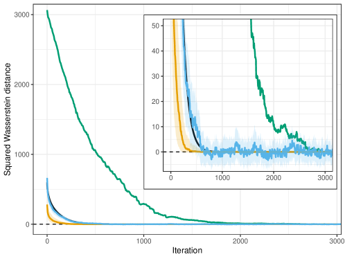
Refer to caption
Figure 5: Estimated bounds on 𝒲22(πt,π)superscriptsubscript𝒲22subscript𝜋𝑡subscript𝜋\mathcal{W}_{2}^{2}(\pi_{t},\pi_{\infty}) for the Gibbs sampler ( U𝑈U; Lsqsubscript𝐿sqL_{\textup{sq}}; coupling; exact). Shaded areas represent 95%percent9595\% jackknife confidence intervals. The inset plot zooms in on the y𝑦y-axis near 0.

Figure 5 shows that the empirical upper bound U𝑈U is close to the true squared distance for all but the first few iterations. This occurs even though the dimension (d=50𝑑50d=50) is relatively large, because the target is approximately confined to a much lower-dimensional manifold, as is explained in more detail in Appendix E.3. The upper bound degenerates into pure noise at large enough iterations t𝑡t. The lower bound appears to be less noisy than the upper bound, but it is also looser than it. The coupling bound is also rather loose relative to the upper bound U𝑈U. For instance, considering the threshold 𝒲22(πt,π)10superscriptsubscript𝒲22subscript𝜋𝑡subscript𝜋10\mathcal{W}_{2}^{2}(\pi_{t},\pi_{\infty})\leq 10, the upper bound U𝑈U reaches this after 500 iterations, while 2000 iterations are required for the coupling bound. The relatively poor performance of the coupling bound is due to the sub-optimal coupling employed. At the cost of additional tuning parameters, a multiscale coupling strategy which employs common random numbers when the chains are far apart, similarly to that in bou-rabee2020coupling for Hamiltonian Monte Carlo, may yield a tighter coupling bound in this example. However, we expect the empirical bound to still provide a noticeable improvement over this.

4.4.2 Dimensional scaling of ULA and MALA

The behaviour of the mixing time of the Metropolis-Adjusted Langevin Algorithm (MALA) and the Unadjusted Langevin Algorithm (ULA) has been extensively studied in the last few years, with particular attention being given to its dimensional dependence. See durmus2019high; li2021sqrt(d); chewi2021optimal; wu2021minimax for recent theoretical contributions to this area. In contrast to theoretical bounds, which may only be informative in the very high-dimensional regime, our empirical bounds are informative in the low-to-moderate dimensional setting as well.

Following Section 3.3 in biswas2019estimating, we bound the mixing time of ULA and MALA on the target π=𝒩d(0,Σ)𝜋subscript𝒩𝑑0Σ\pi=\mathcal{N}_{d}(0,\Sigma), where Σij=0.5|ij|subscriptΣ𝑖𝑗superscript0.5𝑖𝑗\Sigma_{ij}=0.5^{|i-j|}, and the dimension d𝑑d is varied. As opposed to biswas2019estimating, we start from the initial distribution π0=𝒩d(0,3Id)subscript𝜋0subscript𝒩𝑑03subscript𝐼𝑑\pi_{0}=\mathcal{N}_{d}(0,3I_{d}) which satisfies π0cotπsubscript𝜋0cot𝜋\pi_{0}\smash{\overset{\vphantom{a}\smash{\textup{cot}}}{\rightsquigarrow}}\pi (see Appendix E.4 for details). We scale MALA with h=d1/6superscript𝑑16h=d^{-1/6}, for an acceptance rate of around 70%percent7070\%, following the optimal scaling result of roberts1998optimal at stationarity. The step size of ULA is h=0.2d1/40.2superscript𝑑14h=0.2d^{-1/4}, which maintains the stationary distribution of ULA close to π𝜋\pi even as the dimension grows (see durmus2019high, Corollary 9, and durmus2021asymptotic).
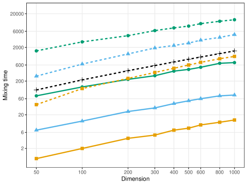
Refer to caption
Figure 6: Estimated mixing time bounds at the 𝒲22(πt,π)6superscriptsubscript𝒲22subscript𝜋𝑡subscript𝜋6\mathcal{W}_{2}^{2}(\pi_{t},\pi_{\infty})\leq 6 threshold ( U𝑈U; Lsqsubscript𝐿sqL_{\textup{sq}}; coupling; exact), for the MALA (solid lines) and ULA (dashed lines). The sequence of targets was Gaussian and satisfied a uniform condition number bound for dimensions d{50,,1000}𝑑501000d\in\{50,\dots,1000\}. Both the y𝑦y- and x𝑥x-axes are on a log10subscript10\log_{10}-scale.

Results are displayed in Figure 6. While theoretical results which apply to our setting (durmus2019high; li2021sqrt(d)) indicate a mixing time bound of O(d1/2log(d))𝑂superscript𝑑12𝑑O(d^{1/2}\log(d)) for ULA, we observe the mixing time to scale closer to d4/5absentsuperscript𝑑45\approx d^{4/5} in our experiment, improving slowly as the dimension is increased. While our largest dimension considered (d=1000𝑑1000d=1000) is relatively large in MCMC contexts, this appears to be relatively small for the asymptotic regime considered in durmus2019high; li2021sqrt(d). Hence, while we expect the trend to approach d1/2log(d)superscript𝑑12𝑑d^{1/2}\log(d) as the dimension becomes large enough, our results suggest that, if only the dimension is considered, theoretical bounds on the mixing time can be misleading in scenarios of practical interest. Given the much larger step size of MALA, it is of no surprise that it converges much faster than ULA. At the same time, in spite of its step size scaling more favorably with the dimension, the mixing time of MALA seems to scale similarly to that of ULA.

The coupling bound suggests a similar scaling of the mixing time with the dimension for both samplers. However, our empirical upper bound improves on the coupling bound by a factor of 333 to 101010 throughout. As the stationary distribution of ULA is overdispersed with respect to the target, our empirical upper and lower bounds can also be used to quantify the bias of ULA at stationarity (see Appendix E.4).

4.4.3 Stochastic volatility model

We investigate the stochastic volatility model in liu2001monte; girolami2011riemann for approximately a year’s worth of data (see Appendix E.5 for details). The hyperparameters are fixed at the true values, and the data are generated from the model. Inference is performed on the latent process conditional on the data, and all samplers are started from the prior distribution of the latent process as sampling from the prior is a frequently used technique to obtain a sample overdispersed with respect to the posterior. This start does not provably satisfy π0cotπsubscript𝜋0cotsubscript𝜋\pi_{0}\smash{\overset{\vphantom{a}\smash{\textup{cot}}}{\rightsquigarrow}}\pi_{\infty}, however a similar bound was obtained from a start which did satisfy the condition (see Appendix E.5), thereby lending credibility to the start-from-the-prior heuristic.
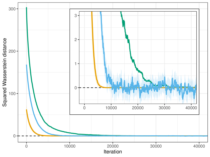
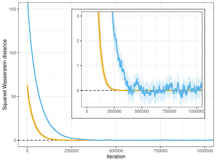
Refer to caption
Refer to caption
Figure 7: Estimated bounds on 𝒲22(πt,π)superscriptsubscript𝒲22subscript𝜋𝑡subscript𝜋\mathcal{W}_{2}^{2}(\pi_{t},\pi_{\infty}) for optimally scaled MALA (left) and RWM (right) on the stochastic volatility model ( U𝑈U; Lsqsubscript𝐿sqL_{\textup{sq}}; coupling). Shaded areas represent 95%percent9595\% jackknife confidence intervals. No coupling bound is computed for the RWM. The inset plots zoom in on the y𝑦y-axis near y=0𝑦0y=0.

Scaling MALA and the RWM optimally for mixing (56%percent5656\% and 24%percent2424\% acceptance rates, respectively), we obtain the results in Figure 7. The empirical bounds suggest that MALA converges more than an order of magnitude quicker than the RWM. The coupling bound is relatively competitive for MALA, although it still suggests a factor of 2 to 3 worse mixing time than the empirical bound. For the RWM, however, the coupled chains coalesce extremely slowly, with 50 pilot chains all failing to meet within 108superscript10810^{8} iterations, and so we are therefore unable to effectively use the coupling bound in this case.
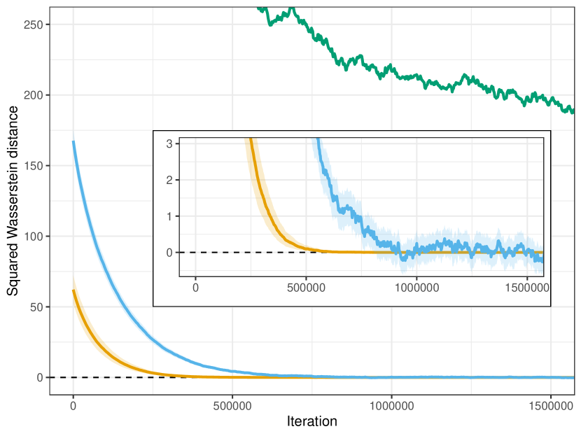
Refer to caption
Refer to caption
Figure 8: Estimated bounds on 𝒲22(πt,π)superscriptsubscript𝒲22subscript𝜋𝑡subscript𝜋\mathcal{W}_{2}^{2}(\pi_{t},\pi_{\infty}) for the RWM with a small scaling, on the stochastic volatility model ( U𝑈U; Lsqsubscript𝐿sqL_{\textup{sq}}; coupling). Shaded areas represent 95%percent9595\% jackknife confidence intervals. Left: zooming in on the empirical bounds, inset plot zooms in further near y=0𝑦0y=0. Right: empirical and coupling bounds, y𝑦y-axis transformed by log10(1+y)subscript101𝑦\log_{10}(1+y), x𝑥x-axis transformed by log10xsubscript10𝑥\log_{10}x.

Lowering the step size of the RWM by a factor of 2.52.52.5 (for an acceptance rate of 64%percent6464\%), the coupled chains now coalesce quicker, and we obtain the results in Figure 8. However, the coupling bound still suggests mixing times more than an order of magnitude larger than the empirical bound does. On the one hand, this shows the different objectives of optimal coalescence with a given coupling and optimal mixing may lead to conflicting tunings for MCMC algorithms. On the other hand, the simulation exposes the difficulty in designing effective practical couplings of Markov chains.

5 Discussion

5.1 General remarks

Under a condition on the Lipschitz constant of the optimal transport map, which we interpret as an overdispersion condition, we show that an upper bound U𝑈U on the squared 2-Wasserstein distance can be obtained by a simple debiasing of the plug-in estimator. This is complemented by a lower bound L𝐿L on the Wasserstein distance, obtained at negligible additional cost. In comparison to the plug-in estimator, the debiased estimator U𝑈U has the advantage of decaying, on average, in proportion to the true Wasserstein distance. When the Wasserstein distance is relatively small, the debiased estimator attains a large improvement in average absolute error. At the same time, similar to the plug-in estimator, the average relative error of the debiased estimator becomes worse as the Wasserstein distance becomes smaller. As our estimator is a linear combination of plug-in estimators, we see no improvement in the rate of convergence to the true Wasserstein distance as the sample size increases. This stresses the fundamental difficulty in accurately estimating the Wasserstein distance from independent samples.

Under a compact support assumption, the point estimators U𝑈U and L𝐿L concentrate around their means with (nearly) sub-Gaussian tails. Coupled with results on the rate of convergence of these estimators under a continuity assumption, the point estimators themselves are seen to be reliable bounds with high probability. Namely, both the probability that U𝑈U is not an upper bound, and the probability that L𝐿L is not a lower bound, decay exponentially quickly in the sample size n𝑛n.

Building on work in mills-tettey2007the, we have suggested a procedure to efficiently compute the jackknife variance estimate to the solution of a linear assignment problem. This applies to empirical transportation costs, and all our suggested estimators. Central limit theorems enable the use of Gaussian jackknife confidence intervals for our estimator U𝑈U of the upper bound (1) on the squared Wasserstein distance. However, uncertainty quantification for our estimator L𝐿L of the lower bound (2) is hampered by a lack of satisfactory limit theorems for the unsquared Wasserstein distance. We leave such limit theorems for future work, and suggest the use of Chebyshev confidence intervals instead.

5.2 MCMC

Our bounds can be used to understand the convergence properties of MCMC algorithms sampling continuous distributions, by running multiple chains which start and remain overdispersed with respect to their stationary distributions. As with the coupling upper bound of biswas2019estimating, our bounds can accurately quantify burn-in, and allow the comparison of various approximate or exact MCMC algorithms targeting the same distribution. Numerically, we find that mixing time upper bounds from our empirical upper bound uniformly improve on those from the coupling bound, even beyond an order of magnitude. The coupling bound requires no overdispersion assumption, and so applies more generally than our empirical upper bound. The usefulness of the coupling bound, however, crucially hinges on how effective the coupling is, and we found the empirical upper bound U𝑈U to be uniformly tighter than the coupling bound in our experiments in Section 4.4. Both the coupling and empirical techniques are embarrassingly parallel, and so are suitable for use in a massively parallel MCMC environment. We believe our bound will prove useful to researchers who wish to empirically compare the convergence of various samplers targeting the same distribution.

Due to the error incurred from discretizing the Langevin dynamics, in our experiment in Section 4.4.2 the stationary distribution of ULA was overdispersed with respect to the stationary distribution of MALA, in terms of our notion of contractive optimal transport. It would be of interest to see if this holds beyond the Gaussian case we have considered, and furthermore whether other approximate algorithms also converge to an overdispersed version of their intended target. If so, our upper bound (1) could be used to quantify the bias of approximate MCMC algorithms more generally.

The potential scale reduction factor R^^𝑅\widehat{R} (gelman1992inference; brooks1998general; see also the recent extension in vehtari2021rank-normalization) is a widely-used heuristic for assessing the convergence of Markov chains. Similarly to our work, the potential scale reduction factor assumes that multiple chains start and remain overdispersed with respect to the target, also considers information between chains, and the scalar statistic R^^𝑅\widehat{R} converges (to a value of one) as the chains approach their limiting distributions. Our work is however better motivated theoretically, as our notion of overdispersion is explicitly defined, if in terms of an abstract condition. Moreover, our bounds are tied to a strong notion of convergence. While weak convergence of the chains is guaranteed by the convergence of the Wasserstein distance to zero, convergence of the potential scale reduction factor to one need not imply weak convergence, even if the Markov chains do not undergo pathological behaviour.

5.3 Additional related work

Very recent work has sought to exploit the smoothness and strong convexity of the Brenier potential in order to analyze the rate of convergence with the sample size n𝑛n of the plug-in Wassertein distance estimator (ghosal2021multivariate; hutter2021minimax; deb2021rates; manole2021plugin), propose estimators with improved rates of convergence under additional smoothness conditions on the potential (hutter2021minimax; deb2021rates; manole2021plugin), and propose new estimation procedures for the Wasserstein distance (paty2020regularity).

In particular, in independent parallel work (manole2021plugin, Proposition 12), a result similar to our Theorem 1 is obtained, under the condition that the Brenier potential is smooth and strongly convex. Termed a “stability bound”, such results have been used to analyze the convergence with the sample size n𝑛n of estimators of Wasserstein distances and transportation costs (ghosal2021multivariate; hutter2021minimax; deb2021rates; manole2021plugin). Our contribution is inherently different, as we use our theoretical results to remove a large portion of the bias of the empirical Wasserstein distance, and also apply our work to accurately quantify the Wasserstein distance in MCMC. Nonetheless, the stability bound of (manole2021plugin, Proposition 12) can be used to prove the upper bound (1). Furthermore, it can be used to show that the rate of convergence of the upper bound estimator is no faster than n2/dsuperscript𝑛2𝑑n^{-2/d} when d5𝑑5d\geq 5 (see Appendix C.1).

5.4 Further work

Our experiments in Section 2.4 suggest that the condition νcotμ𝜈cot𝜇\nu\smash{\overset{\vphantom{a}\smash{\textup{cot}}}{\rightsquigarrow}}\mu is loose for the sufficiency of the upper bound (1). It may be possible to weaken this condition if one only wishes the upper bound (1) to hold for large finite values of n𝑛n.

Uncertainty quantification for the lower bound (2) is hindered by a the lack of a central limit theorem for the term 𝒲2(μ^n,μ^n)subscript𝒲2superscriptsubscript^𝜇𝑛subscript^𝜇𝑛\mathcal{W}_{2}(\hat{\mu}_{n}^{\prime},\hat{\mu}_{n}). Even characterizing when the variance of this statistic decays at a rate faster than 1/n1𝑛1/n would immediately enable much tighter confidence intervals to be computed for the lower bound (2). Results on the validity of the bootstrap for optimal transportation costs in the continuous case are also of interest, since the procedure in sommerfeld2019optimal could be used to efficiently compute both the emprirical transportation cost and its bootstrap sample. Progress here has been made in the case where the distributions are known to be Gaussian (rippl2016limit), although a different estimator of the Wasserstein distance is used.

Investigating whether it is possible to extend bounds of the type (1) to general transportation costs would be of interest. As Brenier’s theorem seems crucial to our characterization of a sufficient condition under which the bound (1) holds, the characterization of the optimal transport map for general costs (gangbo1996the) may prove to be key to the generalization. An extension of the bound (1) to entropic transportation costs would also be of interest. Such extensions would automatically imply stability bounds as in manole2021plugin.

In a multiple-chain MCMC context, the assignment computed with 𝒲22(π^t,π^T)superscriptsubscript𝒲22subscript^𝜋𝑡subscript^𝜋𝑇\mathcal{W}_{2}^{2}(\hat{\pi}_{t},\hat{\pi}_{T}) may contain additional information to complement the empirical bounds. For instance, if one tracks the assignments for iterations t{0,1,}𝑡01t\in\{0,1,\dots\} and observes clustering, that may indicate that the chains are trapped in local modes of the target.

Analytical derivations in the Gaussian case show that the stationary distribution of the ULA is overdispersed with respect to its target, in terms of a Loewner ordering of the covariance matrices. This enables the upper bound (1) to be used to quantify the stationary bias of the ULA. Formally establishing the overdispersion of the stationary distribution of ULA beyond the Gaussian case would increase the applicability of the upper bound (1) to quantify the stationary bias of the ULA. Similarly, it may also be possible to apply the bound (1) to quantify the bias of other types of approximate MCMC algorithms, such as stochastic gradient Markov chain Monte Carlo (e.g. nemeth2021stochastic).

Acknowledgements

This paper is based on work completed while Tamás Papp was part of the EPSRC-funded STOR-i Centre for Doctoral Training (grant EP/S022252/1). Chris Sherlock was supported by EPSRC grant EP/P033075/1.

Supplementary material

The supplementary material contains additional background on optimal transport and convexity (Appendix A), all proofs (Appendix B), a discussion on immediate generalizations of results in the main body of the paper and of selected results related to the proofs (Appendix C), a discussion on extending the methodology in biswas2019estimating to 2-Wasserstein distances (Appendix D), and finally additional details on the numerical experiments (Appendix E).

References

  • Arjovsky et al., (2017) Arjovsky, M., Chintala, S., and Bottou, L. (2017). Wasserstein generative adversarial networks. In Proceedings of the 34th International Conference on Machine Learning, volume 70 of Proceedings of Machine Learning Research, pages 214–223. PMLR.
  • Biswas et al., (2019) Biswas, N., Jacob, P. E., and Vanetti, P. (2019). Estimating convergence of Markov chains with L-lag couplings. In Advances in Neural Information Processing Systems, volume 32, pages 7391–7401.
  • Bobkov and Ledoux, (2019) Bobkov, S. and Ledoux, M. (2019). One-dimensional empirical measures, order statistics, and Kantorovich transport distances. Memoirs of the American Mathematical Society, 261(1259).
  • Bou-Rabee et al., (2020) Bou-Rabee, N., Eberle, A., and Zimmer, R. (2020). Coupling and convergence for Hamiltonian Monte Carlo. The Annals of Applied Probability, 30(3):1209 – 1250.
  • Brenier, (1991) Brenier, Y. (1991). Polar factorization and monotone rearrangement of vector-valued functions. Communications on Pure and Applied Mathematics, 44(4):375–417.
  • Brooks and Gelman, (1998) Brooks, S. P. and Gelman, A. (1998). General methods for monitoring convergence of iterative simulations. Journal of Computational and Graphical Statistics, 7(4):434–455.
  • Caffarelli, (2000) Caffarelli, L. A. (2000). Monotonicity properties of optimal transportation and the FKG and related inequalities. Communications in Mathematical Physics, 214(3):547–563.
  • Chewi et al., (2021) Chewi, S., Lu, C., Ahn, K., Cheng, X., Gouic, T. L., and Rigollet, P. (2021). Optimal dimension dependence of the Metropolis-Adjusted Langevin Algorithm. In Proceedings of Thirty Fourth Conference on Learning Theory, volume 134, pages 1260–1300. PMLR.
  • Chewi and Pooladian, (2022) Chewi, S. and Pooladian, A.-A. (2022). An entropic generalization of Caffarelli’s contraction theorem via covariance inequalities. arXiv preprint arXiv:2203.04954.
  • Chizat et al., (2020) Chizat, L., Roussillon, P., Léger, F., Vialard, F.-X., and Peyré, G. (2020). Faster Wasserstein distance estimation with the Sinkhorn divergence. In Advances in Neural Information Processing Systems, volume 33.
  • Crouse, (2016) Crouse, D. F. (2016). On implementing 2d rectangular assignment algorithms. IEEE Transactions on Aerospace and Electronic Systems, 52(4).
  • Cuturi, (2013) Cuturi, M. (2013). Sinkhorn distances: Lightspeed computation of optimal transport. In Advances in Neural Information Processing Systems, volume 26.
  • Deb et al., (2021) Deb, N., Ghosal, P., and Sen, B. (2021). Rates of estimation of optimal transport maps using plug-in estimators via barycentric projections. arXiv preprint arXiv:2107.01718.
  • del Barrio et al., (2005) del Barrio, E., Giné, E., and Utzet, F. (2005). Asymptotics for L2 functionals of the empirical quantile process, with applications to tests of fit based on weighted Wasserstein distances. Bernoulli, 11(1):131–189.
  • del Barrio et al., (2021) del Barrio, E., González-Sanz, A., and Loubes, J.-M. (2021). Central limit theorems for general transportation costs. arXiv preprint arXiv:2102.06379.
  • del Barrio et al., (2019) del Barrio, E., Gordaliza, P., and Loubes, J.-M. (2019). A central limit theorem for Lpsubscript𝐿𝑝L_{p} transportation cost on the real line with application to fairness assessment in machine learning. Information and Inference: A Journal of the IMA, 8(4):817–849.
  • del Barrio and Loubes, (2019) del Barrio, E. and Loubes, J.-M. (2019). Central limit theorems for empirical transportation cost in general dimension. Annals of Probability, 47(2):926–951.
  • Dowson and Landau, (1982) Dowson, D. and Landau, B. (1982). The fréchet distance between multivariate normal distributions. Journal of Multivariate Analysis, 12(3):450–455.
  • Durmus and Eberle, (2021) Durmus, A. and Eberle, A. (2021). Asymptotic bias of inexact Markov Chain Monte Carlo methods in high dimension. arXiv preprint arXiv:2108.00682.
  • Durmus and Moulines, (2019) Durmus, A. and Moulines, E. (2019). High-dimensional Bayesian inference via the unadjusted Langevin algorithm. Bernoulli, 25(4A):2854–2882.
  • Efron and Stein, (1981) Efron, B. and Stein, C. (1981). The jackknife estimate of variance. The Annals of Statistics, 9(3):586–596.
  • Fathi et al., (2020) Fathi, M., Gozlan, N., and Prod’homme, M. (2020). A proof of the Caffarelli contraction theorem via entropic regularization. Calculus of Variations and Partial Differential Equations, 59(96).
  • Fournier and Guillin, (2015) Fournier, N. and Guillin, A. (2015). On the rate of convergence in Wasserstein distance of the empirical measure. Probability Theory and Related Fields, 162:707–738.
  • Gangbo and McCann, (1996) Gangbo, W. and McCann, R. J. (1996). The geometry of optimal transportation. Acta Mathematica, 177(2):113–161.
  • Gelman and Rubin, (1992) Gelman, A. and Rubin, D. B. (1992). Inference from iterative simulation using multiple sequences. Statistical Science, 7(4):457–472.
  • Ghosal and Sen, (2021) Ghosal, P. and Sen, B. (2021). Multivariate ranks and quantiles using optimal transport: Consistency, rates, and nonparametric testing. Annals of Statistics (to appear).
  • Giovagnoli and Wynn, (1995) Giovagnoli, A. and Wynn, H. P. (1995). Multivariate dispersion orderings. Statistics & Probability Letters, 22(4):325–332.
  • Girolami and Calderhead, (2011) Girolami, M. and Calderhead, B. (2011). Riemann manifold Langevin and Hamiltonian Monte Carlo methods. Journal of the Royal Statistical Society: Series B (Statistical Methodology), 73(2):123–214.
  • Hütter and Rigollet, (2021) Hütter, J.-C. and Rigollet, P. (2021). Minimax estimation of smooth optimal transport maps. The Annals of Statistics, 49(2):1166–1194.
  • Jonker and Volgenant, (1987) Jonker, R. and Volgenant, A. (1987). A shortest augmenting path algorithm for dense and sparse linear assignment problems. Computing, 38(4):325–340.
  • Jonker and Volgenant, (1986) Jonker, R. and Volgenant, T. (1986). Improving the Hungarian assignment algorithm. Operations Research Letters, 5(4):171–175.
  • Kim and Milman, (2012) Kim, Y.-H. and Milman, E. (2012). A generalization of Caffarelli’s contraction theorem via (reverse) heat flow. Mathematische Annalen, 354(3):827–862.
  • Kolesnikov, (2010) Kolesnikov, A. V. (2010). Mass transportation and contractions. Proceedings of the Moscow Institute of Physics and Technology, 2(4):90–99.
  • Kovács, (2015) Kovács, P. (2015). Minimum-cost flow algorithms: an experimental evaluation. Optimization Methods and Software, 30(1):94–127.
  • Kuhn, (1955) Kuhn, H. W. (1955). The Hungarian method for the assignment problem. Naval Research Logistics Quarterly, 2(1-2):83–97.
  • Lei, (2020) Lei, J. (2020). Convergence and concentration of empirical measures under Wasserstein distance in unbounded functional spaces. Bernoulli, 26(1):767–798.
  • Li et al., (2021) Li, R., Zha, H., and Tao, M. (2021). Sqrt(d) dimension dependence of Langevin Monte Carlo. arXiv preprint arXiv:2109.0383.
  • Liu, (2001) Liu, J. S. (2001). Monte Carlo Strategies in Scientific Computing. Springer.
  • Manole et al., (2021) Manole, T., Balakrishnan, S., Niles-Weed, J., and Wasserman, L. (2021). Plugin estimation of smooth optimal transport maps. arXiv preprint arXiv:2107.12364.
  • McCann, (1995) McCann, R. J. (1995). Existence and uniqueness of monotone measure-preserving maps. Duke Mathematical Journal, 80(2):309–323.
  • Mena and Niles-Weed, (2019) Mena, G. and Niles-Weed, J. (2019). Statistical bounds for entropic optimal transport: sample complexity and the central limit theorem. In Advances in Neural Information Processing Systems, volume 32.
  • Mills-Tettey et al., (2007) Mills-Tettey, G. A., Stentz, A., and Dias, M. B. (2007). The dynamic Hungarian algorithm for the assignment problem with changing costs. Technical Report CMU-RI-TR-07-27, Robotics Institute, Carnegie Mellon University.
  • Nadjahi et al., (2020) Nadjahi, K., Durmus, A., Chizat, L., Kolouri, S., Shahrampour, S., and Simsekli, U. (2020). Statistical and topological properties of sliced probability divergences. In Advances in Neural Information Processing Systems, volume 33, pages 20802–20812.
  • Nemeth and Fearnhead, (2021) Nemeth, C. and Fearnhead, P. (2021). Stochastic gradient Markov chain Monte Carlo. Journal of the American Statistical Association, 116(533):433–450.
  • Nietert et al., (2021) Nietert, S., Goldfeld, Z., and Kato, K. (2021). Smooth p𝑝p-Wasserstein distance: Structure, empirical approximation, and statistical applications. In Proceedings of the 38th International Conference on Machine Learning, volume 139 of Proceedings of Machine Learning Research, pages 8172–8183. PMLR.
  • Niles-Weed and Rigollet, (2022) Niles-Weed, J. and Rigollet, P. (2022). Estimation of Wasserstein distances in the Spiked Transport Model. Bernoulli (to appear).
  • Panaretos and Zemel, (2019) Panaretos, V. M. and Zemel, Y. (2019). Statistical aspects of Wasserstein distances. Annual Review of Statistics and Its Application, 6(1):405–431.
  • Paty et al., (2020) Paty, F.-P., d’Aspremont, A., and Cuturi, M. (2020). Regularity as regularization: smooth and strongly convex Brenier potentials in optimal transport. In Proceedings of the Twenty Third International Conference on Artificial Intelligence and Statistics, pages 1222–1232. PMLR.
  • Peyré and Cuturi, (2019) Peyré, G. and Cuturi, M. (2019). Computational optimal transport. Foundations and Trends in Machine Learning, 11(5-6):355–607.
  • Ramdas et al., (2017) Ramdas, A., Trillos, N. G., and Cuturi, M. (2017). On Wasserstein two-sample testing and related families of nonparametric tests. Entropy, 19(2).
  • Rippl et al., (2016) Rippl, T., Munk, A., and Sturm, A. (2016). Limit laws of the empirical Wasserstein distance: Gaussian distributions. Journal of Multivariate Analysis, 151:90–109.
  • Roberts and Rosenthal, (1998) Roberts, G. O. and Rosenthal, J. S. (1998). Optimal scaling of discrete approximations to Langevin diffusions. Journal of the Royal Statistical Society: Series B (Statistical Methodology), 60(1):255–268.
  • Shaked, (1982) Shaked, M. (1982). Dispersive ordering of distributions. Journal of Applied Probability, 19(2):310–320.
  • Shaked and Shanthikumar, (2007) Shaked, M. and Shanthikumar, J. G. (2007). Stochastic Orders. Springer.
  • Sommerfeld and Munk, (2018) Sommerfeld, M. and Munk, A. (2018). Inference for empirical Wasserstein distances on finite spaces. Journal of the Royal Statistical Society: Series B (Statistical Methodology), 80(1):219–238.
  • Sommerfeld et al., (2019) Sommerfeld, M., Schrieber, J., Zemel, Y., and Munk, A. (2019). Optimal transport: Fast probabilistic approximation with exact solvers. Journal of Machine Learning Research, 20(105):1–23.
  • Sriperumbudur et al., (2012) Sriperumbudur, B. K., Fukumizu, K., Gretton, A., Schölkopf, B., and Lanckriet, G. R. G. (2012). On the empirical estimation of integral probability metrics. Electronic Journal of Statistics, 6:1550–1599.
  • Strassen, (1965) Strassen, V. (1965). The existence of probability measures with given marginals. The Annals of Mathematical Statistics, 36(2):423 – 439.
  • Tameling et al., (2019) Tameling, C., Sommerfeld, M., and Munk, A. (2019). Empirical optimal transport on countable metric spaces: Distributional limits and statistical applications. Annals of Applied Probability, 29(5):2744–2781.
  • Valdimarsson, (2007) Valdimarsson, S. I. (2007). On the Hessian of the optimal transport potential. Annali della Scuola Normale Superiore di Pisa - Classe di Scienze, 6(3):441–456.
  • Vehtari et al., (2021) Vehtari, A., Gelman, A., Simpson, D., Carpenter, B., and Bürkner, P.-C. (2021). Rank-normalization, folding, and localization: An improved R^^𝑅\widehat{R} for assessing convergence of MCMC (with discussion). Bayesian Analysis, 16(2):667–718.
  • Villani, (2003) Villani, C. (2003). Topics in Optimal Transportation. Graduate studies in mathematics. American Mathematical Society.
  • Villani, (2009) Villani, C. (2009). Optimal Transport: Old and New. Springer.
  • Weed and Bach, (2019) Weed, J. and Bach, F. (2019). Sharp asymptotic and finite-sample rates of convergence of empirical measures in Wasserstein distance. Bernoulli, 25(4A):2620–2648.
  • Wilkinson, (2020) Wilkinson, D. (2020). Contribution to the discussion of “Unbiased Markov chain Monte Carlo methods with couplings”. Journal of the Royal Statistical Society: Series B (Statistical Methodology), 82(3):543–600.
  • Wu et al., (2021) Wu, K., Schmidler, S., and Chen, Y. (2021). Minimax mixing time of the Metropolis-Adjusted Langevin Algorithm for log-concave sampling. arXiv preprint arXiv:2109.13055.

Appendix A Additional background

A.1 Quadratic optimal transport

The squared Wasserstein distance 𝒲22(μ,ν)superscriptsubscript𝒲22𝜇𝜈\mathcal{W}_{2}^{2}(\mu,\nu) admits a dual formulation (villani2009optimal, Theorem 5.10), which is often easier to manipulate than the primal formulation. Letting Φ={(ψ,ψ~)L1(μ)×L1(ν):ψ(x)ψ~(y)xy2}Φconditional-set𝜓~𝜓superscript𝐿1𝜇superscript𝐿1𝜈𝜓𝑥~𝜓𝑦superscriptdelimited-∥∥𝑥𝑦2\Phi=\big{\{}(\psi,\tilde{\psi})\in L^{1}(\mu)\times L^{1}(\nu):\psi(x)-\tilde{\psi}(y)\leq\lVert x-y\rVert^{2}\big{\}}, the (Kantorovich) dual formulation reads

𝒲22(μ,ν)=sup(ψ,ψ~)Φ(𝔼μψ(X)𝔼νψ~(Y)).superscriptsubscript𝒲22𝜇𝜈subscriptsupremum𝜓~𝜓Φsubscript𝔼𝜇𝜓𝑋subscript𝔼𝜈~𝜓𝑌\mathcal{W}_{2}^{2}(\mu,\nu)=\sup_{(\psi,\tilde{\psi})\in\Phi}\big{(}\mathbb{E}_{\mu}\psi(X)-\mathbb{E}_{\nu}\tilde{\psi}(Y)\big{)}. (6)

When the measures μ=μ^n=i=1nδXi/n𝜇subscript^𝜇𝑛superscriptsubscript𝑖1𝑛subscript𝛿subscript𝑋𝑖𝑛\mu=\hat{\mu}_{n}=\sum_{i=1}^{n}\delta_{X_{i}}/n and ν=ν^n=i=1nδYi/n𝜈subscript^𝜈𝑛superscriptsubscript𝑖1𝑛subscript𝛿subscript𝑌𝑖𝑛\nu=\hat{\nu}_{n}=\sum_{i=1}^{n}\delta_{Y_{i}}/n, the primal formulation of the squared Wasserstein distance 𝒲22(μ^n,ν^n)superscriptsubscript𝒲22subscript^𝜇𝑛subscript^𝜈𝑛\mathcal{W}_{2}^{2}(\hat{\mu}_{n},\hat{\nu}_{n}) can be rewritten in terms a minimization problem over permutations, as follows:

𝒲22(μ^n,ν^n)=minσ𝒮n1ni=1nXiYσ(i)2.superscriptsubscript𝒲22subscript^𝜇𝑛subscript^𝜈𝑛subscript𝜎subscript𝒮𝑛1𝑛superscriptsubscript𝑖1𝑛superscriptdelimited-∥∥subscript𝑋𝑖subscript𝑌𝜎𝑖2\mathcal{W}_{2}^{2}(\hat{\mu}_{n},\hat{\nu}_{n})=\min_{\sigma\in\mathcal{S}_{n}}\frac{1}{n}\sum_{i=1}^{n}\lVert X_{i}-Y_{\sigma(i)}\rVert^{2}. (7)

The optimal coupling for the squared Wasserstein distance 𝒲22(μ^n,ν^n)superscriptsubscript𝒲22subscript^𝜇𝑛subscript^𝜈𝑛\mathcal{W}_{2}^{2}(\hat{\mu}_{n},\hat{\nu}_{n}) is degenerate, in the sense that there exist one or more optimal permutations σ𝒮n𝜎subscript𝒮𝑛\sigma\in\mathcal{S}_{n} mapping the points (X1,,Xn)subscript𝑋1subscript𝑋𝑛(X_{1},\dots,X_{n}) to (Y1,,Yn)subscript𝑌1subscript𝑌𝑛(Y_{1},\dots,Y_{n}).

Another case in which an optimal transport map exists is when the measure μ𝜇\mu is continuous (brenier1991polar; mccann1995existence). Here, the result commonly known as Brenier’s Theorem states that there exists a unique map which transports μ𝜇\mu to ν𝜈\nu which is also the gradient of a convex function, and furthermore that this is the unique optimal transport map. The convex function associated to the map is known as a Brenier potential. If both μ𝜇\mu and ν𝜈\nu are continuous, then there similarly exists an optimal transport map from ν𝜈\nu to μ𝜇\mu, uniquely determined as the gradient of a convex function. In this case, the Brenier potentials are Legendre-Fenchel conjugates of each other (see mccann1995existence, Remark 16). The Legendre-Fenchel conjugate φ~~𝜑\tilde{\varphi} of φ𝜑\varphi is defined as φ~(x)=supy{xTyφ(y)}~𝜑𝑥subscriptsupremum𝑦superscript𝑥𝑇𝑦𝜑𝑦\tilde{\varphi}(x)=\sup_{y}\{x^{T}y-\varphi(y)\}. Theorem 10 below formally states the results described in this paragraph.

Theorem 10 (Brenier’s Theorem).

Let μ,ν𝒫(d)𝜇𝜈𝒫superscript𝑑\mu,\nu\in\mathcal{P}(\mathbb{R}^{d}) have finite second moments.

  1. (i)

    If μ𝜇\mu is continuous, then there exists a convex function φ:d:𝜑superscript𝑑\varphi:\mathbb{R}^{d}\to\mathbb{R} such that its gradient φ𝜑\nabla\varphi pushes μ𝜇\mu forward to ν𝜈\nu. The map φ𝜑\nabla\varphi is dμd𝜇\mathrm{d}\mu-almost everywhere uniquely determined among all gradients of convex functions which push μ𝜇\mu forward to ν𝜈\nu. Furthermore, φ𝜑\nabla\varphi is the optimal transport map.

  2. (ii)

    If furthermore ν𝜈\nu is continuous, then the (convex) Legendre-Fenchel conjugate φ~:d:~𝜑superscript𝑑\tilde{\varphi}:\mathbb{R}^{d}\to\mathbb{R} of φ𝜑\varphi satisfies that its gradient φ~~𝜑\nabla\tilde{\varphi} is the dνd𝜈\mathrm{d}\nu-almost everywhere uniquely determined optimal transport map from ν𝜈\nu to μ𝜇\mu. This map is the inverse of φ𝜑\nabla\varphi in the sense that (φ~φ)(x)=x~𝜑𝜑𝑥𝑥(\nabla\tilde{\varphi}\circ\nabla\varphi)(x)=x for dμd𝜇\mathrm{d}\mu-almost all x𝑥x and (φφ~)(y)=y𝜑~𝜑𝑦𝑦(\nabla\varphi\circ\nabla\tilde{\varphi})(y)=y for dνd𝜈\mathrm{d}\nu-almost all y𝑦y.

We emphasize that, as consequence of Theorem 10, once one finds a map which transports μ𝜇\mu to ν𝜈\nu which is of the form φ𝜑\nabla\varphi with φ𝜑\varphi convex, then one has also found the optimal transport map.

Let us also remark on some subtle technicalities regarding Theorem 10, which will however not pose additional challenges to our later proofs. In Theorem 10, the gradients φ𝜑\nabla\varphi and φ~~𝜑\nabla\tilde{\varphi} may not be defined everywhere on dsuperscript𝑑\mathbb{R}^{d}. As the functions φ,φ~𝜑~𝜑\varphi,\tilde{\varphi} are both convex, the gradients φ,φ~𝜑~𝜑\nabla\varphi,\nabla\tilde{\varphi} are however well-defined dμd𝜇\mathrm{d}\mu-almost everywhere and dνd𝜈\mathrm{d}\nu-almost everywhere, respectively, and so these gradients are also well-defined as push-forward maps. While the transport map φ𝜑\nabla\varphi is unique dμd𝜇\mathrm{d}\mu-almost everywhere, the associated Brenier potential φ𝜑\varphi need not be so in general, although it is unique up to the addition of a constant under mild regularity assumptions (see, for instance, delbarrio2021central, Corollary 2.7).

A.2 Duality between strong convexity and Lipschitz continuous gradient

We call f:d:𝑓superscript𝑑f:\mathbb{R}^{d}\to\mathbb{R} m𝑚m-strongly convex (m>0𝑚0m>0) if there exists a convex g:d:𝑔superscript𝑑g:\mathbb{R}^{d}\to\mathbb{R} such that for all xd𝑥superscript𝑑x\in\mathbb{R}^{d} it holds that f(x)=mx2/2+g(x)𝑓𝑥𝑚superscriptdelimited-∥∥𝑥22𝑔𝑥f(x)=m\lVert x\rVert^{2}/2+g(x).

It is known that, for scalar fields, a duality result exists between strong convexity and Lipschitz continuous gradient (also known as “strong smoothness”). Specifically, a function φ:d:𝜑superscript𝑑\varphi:\mathbb{R}^{d}\to\mathbb{R} is 1/L1𝐿1/L-strongly convex function if and only if its Legendre-Fenchel dual is φ~:d:~𝜑superscript𝑑\tilde{\varphi}:\mathbb{R}^{d}\to\mathbb{R} is differentiable and its gradient φ~~𝜑\nabla\tilde{\varphi} is L𝐿L-Lipschitz. This is essentially proven in kakade2012, with the remark that their definition of strong smoothness is equivalent to the potential φ~~𝜑\tilde{\varphi} being differentiable and its gradient being Lipschitz continuous.

Lemma 1.

Let L>0𝐿0L>0 and φ𝜑\varphi and φ~~𝜑\tilde{\varphi} be convex conjugates. Then, φ𝜑\varphi is (1/L)1𝐿(1/L)-strongly convex if and only if φ~~𝜑\tilde{\varphi} is differentiable and φ~~𝜑\nabla\tilde{\varphi} is L𝐿L-Lipschitz.

We additionally have the following lemma, which characterizes the form of differentiable convex functions with Lipschitz continuous gradient.

Lemma 2.

Let f:d:𝑓superscript𝑑f:\mathbb{R}^{d}\to\mathbb{R} be a differentiable function. If f𝑓\nabla f is 1-Lipschitz, then g(x)=x2/2f(x)𝑔𝑥superscriptdelimited-∥∥𝑥22𝑓𝑥g(x)=\lVert x\rVert^{2}/2-f(x) is convex.

Proof.

The map g(x)=x2/2f(x)𝑔𝑥superscriptdelimited-∥∥𝑥22𝑓𝑥g(x)=\lVert x\rVert^{2}/2-f(x) is differentiable. It suffices to show that is convex. For all x,y𝑥𝑦x,y we have that

(xy)T(g(x)g(y))superscript𝑥𝑦𝑇𝑔𝑥𝑔𝑦\displaystyle(x-y)^{T}(\nabla g(x)-\nabla g(y)) =(xy)T(xy+f(x)f(y))absentsuperscript𝑥𝑦𝑇𝑥𝑦𝑓𝑥𝑓𝑦\displaystyle=(x-y)^{T}(x-y+\nabla f(x)-\nabla f(y))
=xy2(xy)T(f(x)f(y))absentsuperscriptdelimited-∥∥𝑥𝑦2superscript𝑥𝑦𝑇𝑓𝑥𝑓𝑦\displaystyle=\lVert x-y\rVert^{2}-(x-y)^{T}(\nabla f(x)-\nabla f(y))
xy2xyf(x)f(y)absentsuperscriptdelimited-∥∥𝑥𝑦2delimited-∥∥𝑥𝑦delimited-∥∥𝑓𝑥𝑓𝑦\displaystyle\geq\lVert x-y\rVert^{2}-\lVert x-y\rVert\lVert\nabla f(x)-\nabla f(y)\rVert (Cauchy-Schwarz)
xy2xy2=0.absentsuperscriptdelimited-∥∥𝑥𝑦2superscriptdelimited-∥∥𝑥𝑦20\displaystyle\geq\lVert x-y\rVert^{2}-\lVert x-y\rVert^{2}=0. (f𝑓\nabla f is 1-Lipschitz)

By the first-order definition of convexity, g𝑔g is convex, which completes the proof. ∎

Theorem 10 asserts that Brenier potentials are convex conjugates of each other. As a corollary of Lemmas 1 and 2 therefore, the following result characterizes the form of the Brenier potentials when the overdispersion condition νcotμ𝜈cot𝜇\nu\smash{\overset{\vphantom{a}\smash{\textup{cot}}}{\rightsquigarrow}}\mu holds. We shall use it in the proof of Theorem 1.

Corollary 3.

Let φ,φ~𝜑~𝜑\varphi,\tilde{\varphi} be as in Brenier’s theorem. If φ~~𝜑\tilde{\varphi} is differentiable and φ~~𝜑\nabla\tilde{\varphi} 1-Lipschitz, then there exist convex functions f,g:d:𝑓𝑔superscript𝑑f,g:\mathbb{R}^{d}\to\mathbb{R} such that φ(x)=x2/2+f(x)𝜑𝑥superscriptdelimited-∥∥𝑥22𝑓𝑥\varphi(x)=\lVert x\rVert^{2}/2+f(x) and φ~(x)=x2/2g(x)~𝜑𝑥superscriptdelimited-∥∥𝑥22𝑔𝑥\tilde{\varphi}(x)=\lVert x\rVert^{2}/2-g(x).

Proof.

By Lemma 2, φ~(x)=x2/2g(x)~𝜑𝑥superscriptdelimited-∥∥𝑥22𝑔𝑥\tilde{\varphi}(x)=\lVert x\rVert^{2}/2-g(x) for some convex function g𝑔g. Now, by Theorem 10, φ𝜑\varphi and φ~~𝜑\tilde{\varphi} are convex conjugates of each other. Since φ~~𝜑\tilde{\varphi} is differentiable and φ~~𝜑\nabla\tilde{\varphi} is 1-Lipschitz, by Lemma 1 it follows that φ𝜑\varphi is 1-strongly convex. By the definition of strong convexity, it follows that φ(x)=x2/2+f(x)𝜑𝑥superscriptdelimited-∥∥𝑥22𝑓𝑥\varphi(x)=\lVert x\rVert^{2}/2+f(x) for some convex f𝑓f, which completes the proof. ∎

Appendix B Proofs

A key ingredient to our proof of Theorem 1 is the non-negative bias of the empirical squared Wasserstein distance 𝒲22(μ^m,ν^n)superscriptsubscript𝒲22subscript^𝜇𝑚subscript^𝜈𝑛\mathcal{W}_{2}^{2}(\hat{\mu}_{m},\hat{\nu}_{n}). This result also generalizes to arbitrary empirical transportation costs.

Lemma 3.

Let μ,ν𝒫(d)𝜇𝜈𝒫superscript𝑑\mu,\nu\in\mathcal{P}(\mathbb{R}^{d}) be two distributions with finite second moments. For m,n𝑚𝑛m,n\in\mathbb{N}, draw X1,,Xmμsimilar-tosubscript𝑋1subscript𝑋𝑚𝜇X_{1},\dots,X_{m}\sim\mu and Y1,,Ynνsimilar-tosubscript𝑌1subscript𝑌𝑛𝜈Y_{1},\dots,Y_{n}\sim\nu not necessarily independently, and define empirical measures μ^m=i=1mδXi/msubscript^𝜇𝑚superscriptsubscript𝑖1𝑚subscript𝛿subscript𝑋𝑖𝑚\hat{\mu}_{m}=\sum_{i=1}^{m}\delta_{X_{i}}/m and ν^n=i=1nδYi/nsubscript^𝜈𝑛superscriptsubscript𝑖1𝑛subscript𝛿subscript𝑌𝑖𝑛\hat{\nu}_{n}=\sum_{i=1}^{n}\delta_{Y_{i}}/n. Then,

𝔼𝒲22(μ^m,ν^n)𝒲22(μ,ν).𝔼superscriptsubscript𝒲22subscript^𝜇𝑚subscript^𝜈𝑛superscriptsubscript𝒲22𝜇𝜈\mathbb{E}\mathcal{W}_{2}^{2}(\hat{\mu}_{m},\hat{\nu}_{n})\geq\mathcal{W}_{2}^{2}(\mu,\nu).
Proof of Lemma 3.

This is a straightforward consequence of Kantorovich duality. Let

Φ^^Φ\displaystyle\widehat{\Phi} ={(φ,ψ)L1(μ^m)×L1(ν^n):φ(x)ψ(y)xy2},absentconditional-set𝜑𝜓superscript𝐿1subscript^𝜇𝑚superscript𝐿1subscript^𝜈𝑛𝜑𝑥𝜓𝑦superscriptdelimited-∥∥𝑥𝑦2\displaystyle=\left\{(\varphi,\psi)\in L^{1}(\hat{\mu}_{m})\times L^{1}(\hat{\nu}_{n}):\varphi(x)-\psi(y)\leq\lVert x-y\rVert^{2}\right\},
ΦΦ\displaystyle\Phi ={(φ,ψ)L1(μ)×L1(ν):φ(x)ψ(y)xy2}.absentconditional-set𝜑𝜓superscript𝐿1𝜇superscript𝐿1𝜈𝜑𝑥𝜓𝑦superscriptdelimited-∥∥𝑥𝑦2\displaystyle=\left\{(\varphi,\psi)\in L^{1}(\mu)\times L^{1}(\nu):\varphi(x)-\psi(y)\leq\lVert x-y\rVert^{2}\right\}.

As L1(μ)L1(μ^m)superscript𝐿1𝜇superscript𝐿1subscript^𝜇𝑚L^{1}(\mu)\subseteq L^{1}(\hat{\mu}_{m}) and L1(ν)L1(ν^m)superscript𝐿1𝜈superscript𝐿1subscript^𝜈𝑚L^{1}(\nu)\subseteq L^{1}(\hat{\nu}_{m}), we have that Φ^Φ^ΦΦ\widehat{\Phi}\subseteq\Phi. Now, by Kantorovich duality (6),

𝔼𝒲22(μ^m,ν^n)𝔼superscriptsubscript𝒲22subscript^𝜇𝑚subscript^𝜈𝑛\displaystyle\mathbb{E}\mathcal{W}_{2}^{2}(\hat{\mu}_{m},\hat{\nu}_{n}) =𝔼[sup(φ,ψ)Φ^(𝔼μ^mφ(X)𝔼ν^nψ(Y))]absent𝔼delimited-[]𝜑𝜓^Φsupremumsubscript𝔼subscript^𝜇𝑚𝜑𝑋subscript𝔼subscript^𝜈𝑛𝜓𝑌\displaystyle=\mathbb{E}\left[\underset{(\varphi,\psi)\in\widehat{\Phi}}{\sup}\Big{(}\mathbb{E}_{\hat{\mu}_{m}}\varphi(X)-\mathbb{E}_{\hat{\nu}_{n}}\psi(Y)\Bigr{)}\right]
𝔼[sup(φ,ψ)Φ(𝔼μ^mφ(X)𝔼ν^nψ(Y))],absent𝔼delimited-[]𝜑𝜓Φsupremumsubscript𝔼subscript^𝜇𝑚𝜑𝑋subscript𝔼subscript^𝜈𝑛𝜓𝑌\displaystyle\geq\mathbb{E}\left[\underset{(\varphi,\psi)\in\Phi}{\sup}\Big{(}\mathbb{E}_{\hat{\mu}_{m}}\varphi(X)-\mathbb{E}_{\hat{\nu}_{n}}\psi(Y)\Bigr{)}\right], (ΦΦ^Φ^Φ\Phi\subseteq\widehat{\Phi})
which, by the convexity of the supremum and Jensen’s inequality, is
sup(φ,ψ)Φ𝔼(𝔼μ^mφ(X)𝔼ν^nψ(Y))absent𝜑𝜓Φsupremum𝔼subscript𝔼subscript^𝜇𝑚𝜑𝑋subscript𝔼subscript^𝜈𝑛𝜓𝑌\displaystyle\geq\underset{(\varphi,\psi)\in\Phi}{\sup}\mathbb{E}\Bigl{(}\mathbb{E}_{\hat{\mu}_{m}}\varphi(X)-\mathbb{E}_{\hat{\nu}_{n}}\psi(Y)\Bigr{)}
=sup(φ,ψ)Φ(𝔼μφ(X)𝔼νψ(Y))absent𝜑𝜓Φsupremumsubscript𝔼𝜇𝜑𝑋subscript𝔼𝜈𝜓𝑌\displaystyle=\underset{(\varphi,\psi)\in\Phi}{\sup}\Bigl{(}\mathbb{E}_{\mu}\varphi(X)-\mathbb{E}_{\nu}\psi(Y)\Bigr{)}
=𝒲22(μ,ν).absentsuperscriptsubscript𝒲22𝜇𝜈\displaystyle=\mathcal{W}_{2}^{2}(\mu,\nu). (Kantorovich duality)

This completes the proof. ∎

Another key ingredient to the proofs of Theorems 1, 2 and Proposition 1 is the following implication of Assumption 1. As long as μ^nsubscript^𝜇𝑛\hat{\mu}_{n} is independent of both ν^nsubscript^𝜈𝑛\hat{\nu}_{n} and μ^nsuperscriptsubscript^𝜇𝑛\hat{\mu}_{n}^{\prime}, notice that 𝔼𝒲22(ν^n,μ^n)𝔼𝒲22(μ^n,μ^n)𝔼superscriptsubscript𝒲22subscript^𝜈𝑛subscript^𝜇𝑛𝔼superscriptsubscript𝒲22superscriptsubscript^𝜇𝑛subscript^𝜇𝑛\mathbb{E}\mathcal{W}_{2}^{2}(\hat{\nu}_{n},\hat{\mu}_{n})-\mathbb{E}\mathcal{W}_{2}^{2}(\hat{\mu}_{n}^{\prime},\hat{\mu}_{n}) remains the same whether the empirical measures ν^nsubscript^𝜈𝑛\hat{\nu}_{n} and μ^nsuperscriptsubscript^𝜇𝑛\hat{\mu}_{n}^{\prime} are dependent or not. We shall induce a strong dependence between ν^nsubscript^𝜈𝑛\hat{\nu}_{n} and μ^nsuperscriptsubscript^𝜇𝑛\hat{\mu}_{n}^{\prime} by sampling (Xi,Yi)subscript𝑋𝑖subscript𝑌𝑖(X_{i},Y_{i}) from the optimal coupling of μ,ν𝜇𝜈\mu,\nu, independently for all i{1,,n}𝑖1𝑛i\in\{1,\dots,n\}.

B.1 Main results

We prove our main result, Theorem 1, which states empirical bounds on 𝒲22(μ,ν)superscriptsubscript𝒲22𝜇𝜈\mathcal{W}_{2}^{2}(\mu,\nu).

Proof of Theorem 1.

Let X,Zμsimilar-to𝑋𝑍𝜇X,Z\sim\mu and Yνsimilar-to𝑌𝜈Y\sim\nu. To simplify the notation, we drop the subscript n𝑛n from the empirical measures μ^nsubscript^𝜇𝑛\hat{\mu}_{n}, μ^nsubscriptsuperscript^𝜇𝑛\hat{\mu}^{\prime}_{n} and ν^nsubscript^𝜈𝑛\hat{\nu}_{n}, as well as from the set of permutations 𝒮nsubscript𝒮𝑛\mathcal{S}_{n}. Define A=𝒲22(ν^,μ^)𝒲22(μ^,μ^)𝐴superscriptsubscript𝒲22^𝜈^𝜇superscriptsubscript𝒲22superscript^𝜇^𝜇A=\mathcal{W}_{2}^{2}(\hat{\nu},\hat{\mu})-\mathcal{W}_{2}^{2}(\hat{\mu}^{\prime},\hat{\mu}). Let π𝜋\pi be the optimal coupling of μ𝜇\mu and ν𝜈\nu.

The upper bound

By the definition of A𝐴A, and the primal formulation of 𝒲22superscriptsubscript𝒲22\mathcal{W}_{2}^{2},

A𝐴\displaystyle A =minσS1ni=1nYiZσ(i)2minσ𝒮1ni=1nXiZσ(i)2absentsubscript𝜎𝑆1𝑛superscriptsubscript𝑖1𝑛superscriptdelimited-∥∥subscript𝑌𝑖subscript𝑍𝜎𝑖2subscript𝜎𝒮1𝑛superscriptsubscript𝑖1𝑛superscriptdelimited-∥∥subscript𝑋𝑖subscript𝑍𝜎𝑖2\displaystyle=\min_{\sigma\in S}\frac{1}{n}\sum_{i=1}^{n}\lVert Y_{i}-Z_{\sigma(i)}\rVert^{2}-\min_{\sigma\in\mathcal{S}}\frac{1}{n}\sum_{i=1}^{n}\lVert X_{i}-Z_{\sigma(i)}\rVert^{2}
minσ𝒮1ni=1n(YiZσ(i)2XiZσ(i)2),absentsubscript𝜎𝒮1𝑛superscriptsubscript𝑖1𝑛superscriptdelimited-∥∥subscript𝑌𝑖subscript𝑍𝜎𝑖2superscriptdelimited-∥∥subscript𝑋𝑖subscript𝑍𝜎𝑖2\displaystyle\geq\min_{\sigma\in\mathcal{S}}\frac{1}{n}\sum_{i=1}^{n}\left(\lVert Y_{i}-Z_{\sigma(i)}\rVert^{2}-\lVert X_{i}-Z_{\sigma(i)}\rVert^{2}\right), (min\min is concave)
which, by expanding the squared norms, equals
=minσ𝒮1ni=1n(Zσ(i)22(YiXi)TZσ(i)+Yi2Xi2Zσ(i)2).absentsubscript𝜎𝒮1𝑛superscriptsubscript𝑖1𝑛superscriptdelimited-∥∥subscript𝑍𝜎𝑖22superscriptsubscript𝑌𝑖subscript𝑋𝑖𝑇subscript𝑍𝜎𝑖superscriptdelimited-∥∥subscript𝑌𝑖2superscriptdelimited-∥∥subscript𝑋𝑖2superscriptdelimited-∥∥subscript𝑍𝜎𝑖2\displaystyle=\min_{\sigma\in\mathcal{S}}\frac{1}{n}\sum_{i=1}^{n}\left(\lVert Z_{\sigma(i)}\rVert^{2}-2(Y_{i}-X_{i})^{T}Z_{\sigma(i)}+\lVert Y_{i}\rVert^{2}-\lVert X_{i}\rVert^{2}-\lVert Z_{\sigma(i)}\rVert^{2}\right).
Completing the square, then gathering all sums which are invariant to the permutation σ𝜎\sigma, we obtain
=minσ𝒮1ni=1n(YiXi)Zσ(i)21ni=1n(YiXi2Yi2+Zi2+Xi2).absentsubscript𝜎𝒮1𝑛superscriptsubscript𝑖1𝑛superscriptdelimited-∥∥subscript𝑌𝑖subscript𝑋𝑖subscript𝑍𝜎𝑖21𝑛superscriptsubscript𝑖1𝑛superscriptdelimited-∥∥subscript𝑌𝑖subscript𝑋𝑖2superscriptdelimited-∥∥subscript𝑌𝑖2superscriptdelimited-∥∥subscript𝑍𝑖2superscriptdelimited-∥∥subscript𝑋𝑖2\displaystyle=\min_{\sigma\in\mathcal{S}}\frac{1}{n}\sum_{i=1}^{n}\lVert(Y_{i}-X_{i})-Z_{\sigma(i)}\rVert^{2}-\frac{1}{n}\sum_{i=1}^{n}\left(\lVert Y_{i}-X_{i}\rVert^{2}-\lVert Y_{i}\rVert^{2}+\lVert Z_{i}\rVert^{2}+\lVert X_{i}\rVert^{2}\right).

Taking expectations in the above (all expectations are finite by Assumption 1), we obtain

𝔼A𝔼minσ𝒮1ni=1n(YiXi)Zσ(i)2𝔼1ni=1nYiXi2𝔼Z2\Circled1+𝔼Y2𝔼X2\Circled2.𝔼𝐴subscript𝔼subscript𝜎𝒮1𝑛superscriptsubscript𝑖1𝑛superscriptdelimited-∥∥subscript𝑌𝑖subscript𝑋𝑖subscript𝑍𝜎𝑖2𝔼1𝑛superscriptsubscript𝑖1𝑛superscriptdelimited-∥∥subscript𝑌𝑖subscript𝑋𝑖2𝔼superscriptdelimited-∥∥𝑍2\Circled1subscript𝔼superscriptdelimited-∥∥𝑌2𝔼superscriptdelimited-∥∥𝑋2\Circled2\mathbb{E}A\geq\underbrace{\mathbb{E}\min_{\sigma\in\mathcal{S}}\frac{1}{n}\sum_{i=1}^{n}\lVert(Y_{i}-X_{i})-Z_{\sigma(i)}\rVert^{2}-\mathbb{E}\frac{1}{n}\sum_{i=1}^{n}\lVert Y_{i}-X_{i}\rVert^{2}-\mathbb{E}\lVert Z\rVert^{2}}_{\Circled{1}}+\underbrace{\mathbb{E}\lVert Y\rVert^{2}-\mathbb{E}\lVert X\rVert^{2}}_{\Circled{2}}.

We now handle the term \Circled1. By Assumption 1, without changing 𝔼A𝔼𝐴\mathbb{E}A, we choose to sample (Xi,Yi)πsimilar-tosubscript𝑋𝑖subscript𝑌𝑖𝜋(X_{i},Y_{i})\sim\pi independently for all i{1,,n}𝑖1𝑛i\in\{1,\dots,n\}. Since νcotμ𝜈cot𝜇\nu\smash{\overset{\vphantom{a}\smash{\textup{cot}}}{\rightsquigarrow}}\mu, by Corollary 3 there exists a convex f:d:𝑓superscript𝑑f:\mathbb{R}^{d}\to\mathbb{R} such that YiXi=f(Xi)subscript𝑌𝑖subscript𝑋𝑖𝑓subscript𝑋𝑖Y_{i}-X_{i}=\nabla f(X_{i}) for all i{1,,n}𝑖1𝑛i\in\{1,\dots,n\}. We thus have that

\Circled1\Circled1\displaystyle\Circled{1} =𝔼minσ𝒮1ni=1nf(Xi)Zσ(i)2𝔼1ni=1nf(Xi)2𝔼Z2,absent𝔼subscript𝜎𝒮1𝑛superscriptsubscript𝑖1𝑛superscriptdelimited-∥∥𝑓subscript𝑋𝑖subscript𝑍𝜎𝑖2𝔼1𝑛superscriptsubscript𝑖1𝑛superscriptdelimited-∥∥𝑓subscript𝑋𝑖2𝔼superscriptdelimited-∥∥𝑍2\displaystyle=\mathbb{E}\min_{\sigma\in\mathcal{S}}\frac{1}{n}\sum_{i=1}^{n}\lVert\nabla f(X_{i})-Z_{\sigma(i)}\rVert^{2}-\mathbb{E}\frac{1}{n}\sum_{i=1}^{n}\lVert\nabla f(X_{i})\rVert^{2}-\mathbb{E}\lVert Z\rVert^{2},
and introducing the notation ψ=(f)#(μ)𝜓subscript𝑓#𝜇\psi=(\nabla f)_{\#}(\mu) and ψ^=(f)#(μ^)^𝜓subscript𝑓#^𝜇\hat{\psi}=(\nabla f)_{\#}(\hat{\mu}) we can rewrite this as
=𝔼𝒲22(ψ^,μ^)𝔼f(X)2𝔼X2.absent𝔼superscriptsubscript𝒲22^𝜓^𝜇𝔼superscriptdelimited-∥∥𝑓𝑋2𝔼superscriptdelimited-∥∥𝑋2\displaystyle=\mathbb{E}\mathcal{W}_{2}^{2}(\hat{\psi},\hat{\mu})-\mathbb{E}\lVert\nabla f(X)\rVert^{2}-\mathbb{E}\lVert X\rVert^{2}. (X,Zμsimilar-to𝑋𝑍𝜇X,Z\sim\mu)
Now, since f𝑓f is convex and ψ=(f)#(μ)𝜓subscript𝑓#𝜇\psi=(\nabla f)_{\#}(\mu), Brenier’s Theorem 10(i)𝑖(i) says that f𝑓\nabla f is the optimal map which transports μ𝜇\mu to ψ𝜓\psi. It follows that 𝒲22(ψ,μ)=𝔼f(X)2+𝔼X22𝔼f(X)TXsuperscriptsubscript𝒲22𝜓𝜇𝔼superscriptdelimited-∥∥𝑓𝑋2𝔼superscriptdelimited-∥∥𝑋22𝔼𝑓superscript𝑋𝑇𝑋\mathcal{W}_{2}^{2}(\psi,\mu)=\mathbb{E}\lVert\nabla f(X)\rVert^{2}+\mathbb{E}\lVert X\rVert^{2}-2\mathbb{E}\nabla f(X)^{T}X. Hence,
\Circled1\Circled1\displaystyle\Circled{1} =𝔼𝒲22(ψ^,μ^)𝒲22(ψ,μ)2𝔼f(X)TXabsent𝔼superscriptsubscript𝒲22^𝜓^𝜇superscriptsubscript𝒲22𝜓𝜇2𝔼𝑓superscript𝑋𝑇𝑋\displaystyle=\mathbb{E}\mathcal{W}_{2}^{2}(\hat{\psi},\hat{\mu})-\mathcal{W}_{2}^{2}(\psi,\mu)-2\mathbb{E}\nabla f(X)^{T}X
2𝔼f(X)TX.absent2𝔼𝑓superscript𝑋𝑇𝑋\displaystyle\geq-2\mathbb{E}\nabla f(X)^{T}X. (Lemma 3)

For the term \Circled2, we have that

\Circled2\Circled2\displaystyle\Circled{2} =(𝔼Y2+𝔼X2)2𝔼X2absent𝔼superscriptdelimited-∥∥𝑌2𝔼superscriptdelimited-∥∥𝑋22𝔼superscriptdelimited-∥∥𝑋2\displaystyle=\left(\mathbb{E}\lVert Y\rVert^{2}+\mathbb{E}\lVert X\rVert^{2}\right)-2\mathbb{E}\lVert X\rVert^{2}
=𝒲22(μ,ν)+2sup(Y,X)Γ(ν,μ)𝔼YTX2𝔼X2absentsuperscriptsubscript𝒲22𝜇𝜈2subscriptsupremum𝑌𝑋Γ𝜈𝜇𝔼superscript𝑌𝑇𝑋2𝔼superscriptdelimited-∥∥𝑋2\displaystyle=\mathcal{W}_{2}^{2}(\mu,\nu)+2\sup_{(Y,X)\in\Gamma(\nu,\mu)}\mathbb{E}Y^{T}X-2\mathbb{E}\lVert X\rVert^{2}
=𝒲22(μ,ν)+2𝔼(X+f(X))TX2𝔼X2absentsuperscriptsubscript𝒲22𝜇𝜈2𝔼superscript𝑋𝑓𝑋𝑇𝑋2𝔼superscriptdelimited-∥∥𝑋2\displaystyle=\mathcal{W}_{2}^{2}(\mu,\nu)+2\mathbb{E}(X+\nabla f(X))^{T}X-2\mathbb{E}\lVert X\rVert^{2} (Corollary 3)
=𝒲22(μ,ν)+2𝔼f(X)TX.absentsuperscriptsubscript𝒲22𝜇𝜈2𝔼𝑓superscript𝑋𝑇𝑋\displaystyle=\mathcal{W}_{2}^{2}(\mu,\nu)+2\mathbb{E}\nabla f(X)^{T}X.

Overall, we have that

𝔼A\Circled1+\Circled2𝒲22(μ,ν),𝔼𝐴\Circled1\Circled2superscriptsubscript𝒲22𝜇𝜈\mathbb{E}A\geq\Circled{1}+\Circled{2}\geq\mathcal{W}_{2}^{2}(\mu,\nu),

which concludes the proof of the upper bound.

The lower bound

The proof of the lower bounds follows the same structure as that of the upper bound. We first begin by exploiting the symmetry in the expression for A𝐴A, namely

A𝐴\displaystyle A =minσS1ni=1nYiZσ(i)2minσ𝒮1ni=1nXiZσ(i)2absentsubscript𝜎𝑆1𝑛superscriptsubscript𝑖1𝑛superscriptdelimited-∥∥subscript𝑌𝑖subscript𝑍𝜎𝑖2subscript𝜎𝒮1𝑛superscriptsubscript𝑖1𝑛superscriptdelimited-∥∥subscript𝑋𝑖subscript𝑍𝜎𝑖2\displaystyle=\min_{\sigma\in S}\frac{1}{n}\sum_{i=1}^{n}\lVert Y_{i}-Z_{\sigma(i)}\rVert^{2}-\min_{\sigma\in\mathcal{S}}\frac{1}{n}\sum_{i=1}^{n}\lVert X_{i}-Z_{\sigma(i)}\rVert^{2}
=(minσS1ni=1nXiZσ(i)2minσ𝒮1ni=1nYiZσ(i)2),absentsubscript𝜎𝑆1𝑛superscriptsubscript𝑖1𝑛superscriptdelimited-∥∥subscript𝑋𝑖subscript𝑍𝜎𝑖2subscript𝜎𝒮1𝑛superscriptsubscript𝑖1𝑛superscriptdelimited-∥∥subscript𝑌𝑖subscript𝑍𝜎𝑖2\displaystyle=-\left(\min_{\sigma\in S}\frac{1}{n}\sum_{i=1}^{n}\lVert X_{i}-Z_{\sigma(i)}\rVert^{2}-\min_{\sigma\in\mathcal{S}}\frac{1}{n}\sum_{i=1}^{n}\lVert Y_{i}-Z_{\sigma(i)}\rVert^{2}\right),
which, retracing the initial steps of the upper bound proof with Xisubscript𝑋𝑖X_{i} and Yisubscript𝑌𝑖Y_{i} swapped, is
1ni=1n(XiYi2Xi2+Zi2+Yi2)minσ𝒮1ni=1n(XiYi)Zσ(i)2.absent1𝑛superscriptsubscript𝑖1𝑛superscriptdelimited-∥∥subscript𝑋𝑖subscript𝑌𝑖2superscriptdelimited-∥∥subscript𝑋𝑖2superscriptdelimited-∥∥subscript𝑍𝑖2superscriptdelimited-∥∥subscript𝑌𝑖2subscript𝜎𝒮1𝑛superscriptsubscript𝑖1𝑛superscriptdelimited-∥∥subscript𝑋𝑖subscript𝑌𝑖subscript𝑍𝜎𝑖2\displaystyle\leq\frac{1}{n}\sum_{i=1}^{n}\left(\lVert X_{i}-Y_{i}\rVert^{2}-\lVert X_{i}\rVert^{2}+\lVert Z_{i}\rVert^{2}+\lVert Y_{i}\rVert^{2}\right)-\min_{\sigma\in\mathcal{S}}\frac{1}{n}\sum_{i=1}^{n}\lVert(X_{i}-Y_{i})-Z_{\sigma(i)}\rVert^{2}.

Take expectations to obtain

𝔼A𝔼1ni=1nXiYi2+𝔼Z2𝔼minσ𝒮1ni=1n(XiYi)Zσ(i)2\Circled3+𝔼Y2𝔼X2\Circled2.𝔼𝐴subscript𝔼1𝑛superscriptsubscript𝑖1𝑛superscriptdelimited-∥∥subscript𝑋𝑖subscript𝑌𝑖2𝔼superscriptdelimited-∥∥𝑍2𝔼subscript𝜎𝒮1𝑛superscriptsubscript𝑖1𝑛superscriptdelimited-∥∥subscript𝑋𝑖subscript𝑌𝑖subscript𝑍𝜎𝑖2\Circled3subscript𝔼superscriptdelimited-∥∥𝑌2𝔼superscriptdelimited-∥∥𝑋2\Circled2\mathbb{E}A\leq\underbrace{\mathbb{E}\frac{1}{n}\sum_{i=1}^{n}\lVert X_{i}-Y_{i}\rVert^{2}+\mathbb{E}\lVert Z\rVert^{2}-\mathbb{E}\min_{\sigma\in\mathcal{S}}\frac{1}{n}\sum_{i=1}^{n}\lVert(X_{i}-Y_{i})-Z_{\sigma(i)}\rVert^{2}}_{\Circled{3}}+\underbrace{\mathbb{E}\lVert Y\rVert^{2}-\mathbb{E}\lVert X\rVert^{2}}_{\Circled{2}}.

Again, to deal with the term \Circled3, we sample (Xi,Yi)πsimilar-tosubscript𝑋𝑖subscript𝑌𝑖𝜋(X_{i},Y_{i})\sim\pi independently for all i{1,,n}𝑖1𝑛i\in\{1,\dots,n\}. This choice does not change 𝔼A𝔼𝐴\mathbb{E}A. Since μcotν𝜇cot𝜈\mu\overset{\vphantom{a}\smash{\textup{cot}}}{\rightsquigarrow}\nu, by Corollary 3 there exists a convex g:d:𝑔superscript𝑑g:\mathbb{R}^{d}\to\mathbb{R} such that Yi=Xig(Xi)subscript𝑌𝑖subscript𝑋𝑖𝑔subscript𝑋𝑖Y_{i}=X_{i}-\nabla g(X_{i}) for all i{1,,n}𝑖1𝑛i\in\{1,\dots,n\}. Hence, term \Circled3 reduces to

\Circled3\Circled3\displaystyle\Circled{3} =𝔼1ni=1ng(Xi)2+𝔼Z2𝔼minσ𝒮1ni=1ng(Xi)Zσ(i)2.absent𝔼1𝑛superscriptsubscript𝑖1𝑛superscriptdelimited-∥∥𝑔subscript𝑋𝑖2𝔼superscriptdelimited-∥∥𝑍2𝔼subscript𝜎𝒮1𝑛superscriptsubscript𝑖1𝑛superscriptdelimited-∥∥𝑔subscript𝑋𝑖subscript𝑍𝜎𝑖2\displaystyle=\mathbb{E}\frac{1}{n}\sum_{i=1}^{n}\lVert\nabla g(X_{i})\rVert^{2}+\mathbb{E}\lVert Z\rVert^{2}-\mathbb{E}\min_{\sigma\in\mathcal{S}}\frac{1}{n}\sum_{i=1}^{n}\lVert\nabla g(X_{i})-Z_{\sigma(i)}\rVert^{2}.
As with term \Circled1 in the proof for the upper bound, we call ξ=g#(μ)𝜉subscript𝑔#𝜇\xi=\nabla g_{\#}(\mu) and ξ^=g#(μ^)^𝜉subscript𝑔#^𝜇\hat{\xi}=\nabla g_{\#}(\hat{\mu}). By Brenier’s theorem g𝑔\nabla g is the optimal transport map from μ𝜇\mu to ξ𝜉\xi, so
\Circled3\Circled3\displaystyle\Circled{3} =2𝔼g(X)TX+𝒲22(ξ,μ)𝔼𝒲22(ξ^,μ^)absent2𝔼𝑔superscript𝑋𝑇𝑋superscriptsubscript𝒲22𝜉𝜇𝔼superscriptsubscript𝒲22^𝜉^𝜇\displaystyle=2\mathbb{E}\nabla g(X)^{T}X+\mathcal{W}_{2}^{2}(\xi,\mu)-\mathbb{E}\mathcal{W}_{2}^{2}(\hat{\xi},\hat{\mu})
2𝔼g(X)TX.absent2𝔼𝑔superscript𝑋𝑇𝑋\displaystyle\leq 2\mathbb{E}\nabla g(X)^{T}X. (Lemma 3)

Term \Circled2 has appeared in the upper bound proof, it equals

\Circled2\Circled2\displaystyle\Circled{2} =𝒲22(μ,ν)+2sup(Y,X)Γ(ν,μ)𝔼YTX2𝔼X2absentsuperscriptsubscript𝒲22𝜇𝜈2subscriptsupremum𝑌𝑋Γ𝜈𝜇𝔼superscript𝑌𝑇𝑋2𝔼superscriptdelimited-∥∥𝑋2\displaystyle=\mathcal{W}_{2}^{2}(\mu,\nu)+2\sup_{(Y,X)\in\Gamma(\nu,\mu)}\mathbb{E}Y^{T}X-2\mathbb{E}\lVert X\rVert^{2}
=𝒲22(μ,ν)+2𝔼(Xg(X))TX2𝔼X2absentsuperscriptsubscript𝒲22𝜇𝜈2𝔼superscript𝑋𝑔𝑋𝑇𝑋2𝔼superscriptdelimited-∥∥𝑋2\displaystyle=\mathcal{W}_{2}^{2}(\mu,\nu)+2\mathbb{E}(X-\nabla g(X))^{T}X-2\mathbb{E}\lVert X\rVert^{2} (Corollary 3)
=𝒲22(μ,ν)2𝔼g(X)TX.absentsuperscriptsubscript𝒲22𝜇𝜈2𝔼𝑔superscript𝑋𝑇𝑋\displaystyle=\mathcal{W}_{2}^{2}(\mu,\nu)-2\mathbb{E}\nabla g(X)^{T}X.

Altogether, we have that

𝔼A\Circled3+\Circled2𝒲22(μ,ν),𝔼𝐴\Circled3\Circled2superscriptsubscript𝒲22𝜇𝜈\mathbb{E}A\leq\Circled{3}+\Circled{2}\leq\mathcal{W}_{2}^{2}(\mu,\nu),

which concludes the proof of the lower bound. ∎

Next, we prove Proposition 1, which asserts that the upper bound of Theorem 1 decays in proportion to the Wasserstein distance 𝒲2(μ,ν)subscript𝒲2𝜇𝜈\mathcal{W}_{2}(\mu,\nu).

Proof of Proposition 1.

Let X,Zμsimilar-to𝑋𝑍𝜇X,Z\sim\mu and Yνsimilar-to𝑌𝜈Y\sim\nu. To simplify the notation, we drop the subscript n𝑛n from the empirical measures μ^nsubscript^𝜇𝑛\hat{\mu}_{n}, μ^nsubscriptsuperscript^𝜇𝑛\hat{\mu}^{\prime}_{n} and ν^nsubscript^𝜈𝑛\hat{\nu}_{n}, as well as from the set of permutations 𝒮nsubscript𝒮𝑛\mathcal{S}_{n}. Define A=𝒲22(ν^,μ^)𝒲22(μ^,μ^)𝐴superscriptsubscript𝒲22^𝜈^𝜇superscriptsubscript𝒲22superscript^𝜇^𝜇A=\mathcal{W}_{2}^{2}(\hat{\nu},\hat{\mu})-\mathcal{W}_{2}^{2}(\hat{\mu}^{\prime},\hat{\mu}). Let π𝜋\pi be the optimal coupling of μ𝜇\mu and ν𝜈\nu. Recall that μ^=i=1nδXi/nsuperscript^𝜇superscriptsubscript𝑖1𝑛subscript𝛿subscript𝑋𝑖𝑛\hat{\mu}^{\prime}=\sum_{i=1}^{n}\delta_{X_{i}}/n and ν^=i=1nδYi/n^𝜈superscriptsubscript𝑖1𝑛subscript𝛿subscript𝑌𝑖𝑛\hat{\nu}=\sum_{i=1}^{n}\delta_{Y_{i}}/n. By Assumption 1, 𝔼A𝔼𝐴\mathbb{E}A is invariant to choosing (Xi,Yi)πsimilar-tosubscript𝑋𝑖subscript𝑌𝑖𝜋(X_{i},Y_{i})\sim\pi for all i{1,,n}𝑖1𝑛i\in\{1,\dots,n\}, where π𝜋\pi is the optimal coupling of μ𝜇\mu and ν𝜈\nu. In what follows, we make this choice.

𝔼A𝔼𝐴\displaystyle\mathbb{E}A =𝔼Y2𝔼X2+2𝔼(maxσ𝒮1ni=1nXiTZσ(i)maxσ𝒮1ni=1nYiTZσ(i))absent𝔼superscriptdelimited-∥∥𝑌2𝔼superscriptdelimited-∥∥𝑋22𝔼subscript𝜎𝒮1𝑛superscriptsubscript𝑖1𝑛superscriptsubscript𝑋𝑖𝑇subscript𝑍𝜎𝑖subscript𝜎𝒮1𝑛superscriptsubscript𝑖1𝑛superscriptsubscript𝑌𝑖𝑇subscript𝑍𝜎𝑖\displaystyle=\mathbb{E}\lVert Y\rVert^{2}-\mathbb{E}\lVert X\rVert^{2}+2\mathbb{E}\left(\max_{\sigma\in\mathcal{S}}\frac{1}{n}\sum_{i=1}^{n}X_{i}^{T}Z_{\sigma(i)}-\max_{\sigma\in\mathcal{S}}\frac{1}{n}\sum_{i=1}^{n}Y_{i}^{T}Z_{\sigma(i)}\right)
𝔼Y2𝔼X2\Circled1+2𝔼maxσS1ni=1n(XiYi)TZσ(i)\Circled2.absentsubscript𝔼superscriptdelimited-∥∥𝑌2𝔼superscriptdelimited-∥∥𝑋2\Circled12subscript𝔼subscript𝜎𝑆1𝑛superscriptsubscript𝑖1𝑛superscriptsubscript𝑋𝑖subscript𝑌𝑖𝑇subscript𝑍𝜎𝑖\Circled2\displaystyle\leq\underbrace{\mathbb{E}\lVert Y\rVert^{2}-\mathbb{E}\lVert X\rVert^{2}}_{\Circled{1}}+2\underbrace{\mathbb{E}\max_{\sigma\in S}\frac{1}{n}\sum_{i=1}^{n}(X_{i}-Y_{i})^{T}Z_{\sigma(i)}}_{\Circled{2}}. (convexity of max\max)

The term \Circled1 is invariant to the coupling of X𝑋X and Y𝑌Y. Without loss of generality, assume (X,Y)πsimilar-to𝑋𝑌𝜋(X,Y)\sim\pi. Then,

\Circled1\Circled1\displaystyle\Circled{1} =𝔼(YX)T(Y+X)absent𝔼superscript𝑌𝑋𝑇𝑌𝑋\displaystyle=\mathbb{E}(Y-X)^{T}(Y+X)
𝔼YXY+Xabsent𝔼delimited-∥∥𝑌𝑋delimited-∥∥𝑌𝑋\displaystyle\leq\mathbb{E}\lVert Y-X\rVert\lVert Y+X\rVert (Cauchy-Schwarz)
(𝔼YX2)1/2(𝔼Y+X2)1/2absentsuperscript𝔼superscriptdelimited-∥∥𝑌𝑋212superscript𝔼superscriptdelimited-∥∥𝑌𝑋212\displaystyle\leq\left(\mathbb{E}\lVert Y-X\rVert^{2}\right)^{1/2}\left(\mathbb{E}\lVert Y+X\rVert^{2}\right)^{1/2} (Cauchy-Schwarz)
=𝒲2(μ,ν)(𝔼Y+X2)1/2absentsubscript𝒲2𝜇𝜈superscript𝔼superscriptdelimited-∥∥𝑌𝑋212\displaystyle=\mathcal{W}_{2}(\mu,\nu)\left(\mathbb{E}\lVert Y+X\rVert^{2}\right)^{1/2}
=𝒲2(μ,ν)(𝔼Y2+2𝔼XTY+𝔼X2)1/2absentsubscript𝒲2𝜇𝜈superscript𝔼superscriptdelimited-∥∥𝑌22𝔼superscript𝑋𝑇𝑌𝔼superscriptdelimited-∥∥𝑋212\displaystyle=\mathcal{W}_{2}(\mu,\nu)\left(\mathbb{E}\lVert Y\rVert^{2}+2\mathbb{E}X^{T}Y+\mathbb{E}\lVert X\rVert^{2}\right)^{1/2}
𝒲2(μ,ν)(𝔼Y2+2𝔼XY+𝔼X2)1/2absentsubscript𝒲2𝜇𝜈superscript𝔼superscriptdelimited-∥∥𝑌22𝔼delimited-∥∥𝑋delimited-∥∥𝑌𝔼superscriptdelimited-∥∥𝑋212\displaystyle\leq\mathcal{W}_{2}(\mu,\nu)\left(\mathbb{E}\lVert Y\rVert^{2}+2\mathbb{E}\lVert X\rVert\lVert Y\rVert+\mathbb{E}\lVert X\rVert^{2}\right)^{1/2} (Cauchy-Schwarz)
𝒲2(μ,ν)[𝔼Y2+2(𝔼X2𝔼Y2)1/2+𝔼X2]1/2absentsubscript𝒲2𝜇𝜈superscriptdelimited-[]𝔼superscriptdelimited-∥∥𝑌22superscript𝔼superscriptdelimited-∥∥𝑋2𝔼superscriptdelimited-∥∥𝑌212𝔼superscriptdelimited-∥∥𝑋212\displaystyle\leq\mathcal{W}_{2}(\mu,\nu)\left[\mathbb{E}\lVert Y\rVert^{2}+2(\mathbb{E}\lVert X\rVert^{2}\mathbb{E}\lVert Y\rVert^{2})^{1/2}+\mathbb{E}\lVert X\rVert^{2}\right]^{1/2} (Cauchy-Schwarz)
=𝒲2(μ,ν)[(𝔼X2)1/2+(𝔼Y2)1/2].absentsubscript𝒲2𝜇𝜈delimited-[]superscript𝔼superscriptdelimited-∥∥𝑋212superscript𝔼superscriptdelimited-∥∥𝑌212\displaystyle=\mathcal{W}_{2}(\mu,\nu)\left[(\mathbb{E}\lVert X\rVert^{2})^{1/2}+(\mathbb{E}\lVert Y\rVert^{2})^{1/2}\right].

For term \Circled2,

\Circled2\Circled2\displaystyle\Circled{2} 2𝔼maxσS1ni=1nXiYiZσ(i)absent2𝔼subscript𝜎𝑆1𝑛superscriptsubscript𝑖1𝑛delimited-∥∥subscript𝑋𝑖subscript𝑌𝑖delimited-∥∥subscript𝑍𝜎𝑖\displaystyle\leq 2\mathbb{E}\max_{\sigma\in S}\frac{1}{n}\sum_{i=1}^{n}\lVert X_{i}-Y_{i}\rVert\lVert Z_{\sigma(i)}\rVert (Cauchy-Schwarz)
2𝔼maxσS(1ni=1nXiYi2)1/2(1ni=1nZσ(i)2)1/2\displaystyle\leq 2\mathbb{E}\max_{\sigma\in S}\left(\frac{1}{n}\sum_{i=1}^{n}\lVert X_{i}-Y_{i}\rVert^{2}\right)^{1/2}\left(\frac{1}{n}\sum_{i=1}^{n}\lVert Z_{\sigma(i)}\rVert^{2}\right)^{1/2} (Cauchy-Schwarz)
=2𝔼(1ni=1nXiYi2)1/2(1ni=1nZi2)1/2absent2𝔼superscript1𝑛superscriptsubscript𝑖1𝑛superscriptdelimited-∥∥subscript𝑋𝑖subscript𝑌𝑖212superscript1𝑛superscriptsubscript𝑖1𝑛superscriptdelimited-∥∥subscript𝑍𝑖212\displaystyle=2\mathbb{E}\left(\frac{1}{n}\sum_{i=1}^{n}\lVert X_{i}-Y_{i}\rVert^{2}\right)^{1/2}\left(\frac{1}{n}\sum_{i=1}^{n}\lVert Z_{i}\rVert^{2}\right)^{1/2} (σ𝜎\sigma is a permutation)
=2𝔼(1ni=1nXiYi2)1/2𝔼(1ni=1nZi2)1/2,absent2𝔼superscript1𝑛superscriptsubscript𝑖1𝑛superscriptdelimited-∥∥subscript𝑋𝑖subscript𝑌𝑖212𝔼superscript1𝑛superscriptsubscript𝑖1𝑛superscriptdelimited-∥∥subscript𝑍𝑖212\displaystyle=2\mathbb{E}\left(\frac{1}{n}\sum_{i=1}^{n}\lVert X_{i}-Y_{i}\rVert^{2}\right)^{1/2}\mathbb{E}\left(\frac{1}{n}\sum_{i=1}^{n}\lVert Z_{i}\rVert^{2}\right)^{1/2}, (independence)
and letting (X,Y)πsimilar-to𝑋𝑌𝜋(X,Y)\sim\pi, this writes as
=2(𝔼XY2)1/2(𝔼Z2)1/2,absent2superscript𝔼superscriptdelimited-∥∥𝑋𝑌212superscript𝔼superscriptdelimited-∥∥𝑍212\displaystyle=2\left(\mathbb{E}\lVert X-Y\rVert^{2}\right)^{1/2}\left(\mathbb{E}\lVert Z\rVert^{2}\right)^{1/2},
which, since (X,Y)πsimilar-to𝑋𝑌𝜋(X,Y)\sim\pi and X,Zμsimilar-to𝑋𝑍𝜇X,Z\sim\mu, equals
=2𝒲2(μ,ν)(𝔼X2)1/2.absent2subscript𝒲2𝜇𝜈superscript𝔼superscriptdelimited-∥∥𝑋212\displaystyle=2\mathcal{W}_{2}(\mu,\nu)\left(\mathbb{E}\lVert X\rVert^{2}\right)^{1/2}.

Altogether,

𝔼A\Circled1+\Circled2𝒲2(μ,ν)[3(𝔼X2)1/2+𝔼(Y2)1/2],𝔼𝐴\Circled1\Circled2subscript𝒲2𝜇𝜈delimited-[]3superscript𝔼superscriptdelimited-∥∥𝑋212𝔼superscriptsuperscriptdelimited-∥∥𝑌212\mathbb{E}A\leq\Circled{1}+\Circled{2}\leq\mathcal{W}_{2}(\mu,\nu)\left[3(\mathbb{E}\lVert X\rVert^{2})^{1/2}+\mathbb{E}(\lVert Y\rVert^{2})^{1/2}\right],

which completes the proof. ∎

We now turn to Theorem 2, which asserts an empirical lower bound on 𝒲2(μ,ν)subscript𝒲2𝜇𝜈\mathcal{W}_{2}(\mu,\nu).

Proof of Theorem 2.

Drop the subscripts from the empirical measures μ^nsubscript^𝜇𝑛\hat{\mu}_{n}, ν^nsubscript^𝜈𝑛\hat{\nu}_{n}, and the set of permutations 𝒮nsubscript𝒮𝑛\mathcal{S}_{n}. Notice that the independence assumption on φ𝜑\varphi makes |𝔼𝒲2(ν^,μ^)𝔼𝒲2(μ^,μ^)|𝔼subscript𝒲2^𝜈^𝜇𝔼subscript𝒲2superscript^𝜇^𝜇|\mathbb{E}\mathcal{W}_{2}(\hat{\nu},\hat{\mu})-\mathbb{E}\mathcal{W}_{2}(\hat{\mu}^{\prime},\hat{\mu})| invariant to the dependence between ν^^𝜈\hat{\nu} and μ^^𝜇\hat{\mu}. We shall induce a strong dependence between these measures by coupling samples optimally.

By the triangle inequality,

𝒲2(ν^,μ^)𝒲2(μ^,μ^)𝒲2(μ^,ν^).subscript𝒲2^𝜈^𝜇subscript𝒲2superscript^𝜇^𝜇subscript𝒲2superscript^𝜇^𝜈\mathcal{W}_{2}(\hat{\nu},\hat{\mu})-\mathcal{W}_{2}(\hat{\mu}^{\prime},\hat{\mu})\leq\mathcal{W}_{2}(\hat{\mu}^{\prime},\hat{\nu}).

Taking expectations, and noting that the expression also holds with μ^superscript^𝜇\hat{\mu}^{\prime} and ν^^𝜈\hat{\nu} swapped,

|𝔼𝒲2(ν^,μ^)𝔼𝒲2(μ^,μ^)|𝔼𝒲2(μ^,ν^)𝔼subscript𝒲2^𝜈^𝜇𝔼subscript𝒲2superscript^𝜇^𝜇𝔼subscript𝒲2superscript^𝜇^𝜈|\mathbb{E}\mathcal{W}_{2}(\hat{\nu},\hat{\mu})-\mathbb{E}\mathcal{W}_{2}(\hat{\mu}^{\prime},\hat{\mu})|\leq\mathbb{E}\mathcal{W}_{2}(\hat{\mu}^{\prime},\hat{\nu}) (8)

Let π𝜋\pi be the optimal coupling of μ,ν𝜇𝜈\mu,\nu. As |𝔼𝒲2(ν^,μ^)𝔼𝒲2(μ^,μ^)|𝔼subscript𝒲2^𝜈^𝜇𝔼subscript𝒲2superscript^𝜇^𝜇|\mathbb{E}\mathcal{W}_{2}(\hat{\nu},\hat{\mu})-\mathbb{E}\mathcal{W}_{2}(\hat{\mu}^{\prime},\hat{\mu})| is invariant to the dependence between ν^^𝜈\hat{\nu} and μ^superscript^𝜇\hat{\mu}^{\prime}, without changing the left-hand-side of inequality (8), we choose to sample (Xi,Yi)πsimilar-tosubscript𝑋𝑖subscript𝑌𝑖𝜋(X_{i},Y_{i})\sim\pi independently for all i{1,,n}𝑖1𝑛i\in\{1,\dots,n\}, where π𝜋\pi is the optimal coupling of μ𝜇\mu and ν𝜈\nu. Then,

𝔼𝒲2(μ^,ν^)𝔼subscript𝒲2superscript^𝜇^𝜈\displaystyle\mathbb{E}\mathcal{W}_{2}(\hat{\mu}^{\prime},\hat{\nu}) =𝔼(minσS1ni=1nXiYσ(i)2)1/2absent𝔼superscriptsubscript𝜎𝑆1𝑛superscriptsubscript𝑖1𝑛superscriptdelimited-∥∥subscript𝑋𝑖subscript𝑌𝜎𝑖212\displaystyle=\mathbb{E}\left(\min_{\sigma\in S}\frac{1}{n}\sum_{i=1}^{n}\lVert X_{i}-Y_{\sigma(i)}\rVert^{2}\right)^{1/2}
𝔼(1ni=1nXiYi2)1/2absent𝔼superscript1𝑛superscriptsubscript𝑖1𝑛superscriptdelimited-∥∥subscript𝑋𝑖subscript𝑌𝑖212\displaystyle\leq\mathbb{E}\left(\frac{1}{n}\sum_{i=1}^{n}\lVert X_{i}-Y_{i}\rVert^{2}\right)^{1/2}
(𝔼1ni=1nXiYi2)1/2absentsuperscript𝔼1𝑛superscriptsubscript𝑖1𝑛superscriptdelimited-∥∥subscript𝑋𝑖subscript𝑌𝑖212\displaystyle\leq\left(\mathbb{E}\frac{1}{n}\sum_{i=1}^{n}\lVert X_{i}-Y_{i}\rVert^{2}\right)^{1/2} (Jensen’s inequality)
=(𝔼(X,Y)πXY2)1/2=𝒲2(μ,ν).absentsuperscriptsubscript𝔼similar-to𝑋𝑌𝜋superscriptdelimited-∥∥𝑋𝑌212subscript𝒲2𝜇𝜈\displaystyle=\left(\mathbb{E}_{(X,Y)\sim\pi}\lVert X-Y\rVert^{2}\right)^{1/2}=\mathcal{W}_{2}(\mu,\nu). (9)

Combining inequalities (8) and (9), we have that

|𝔼𝒲2(ν^,μ^)𝔼𝒲2(μ^,μ^)|𝔼𝒲2(μ,ν),𝔼subscript𝒲2^𝜈^𝜇𝔼subscript𝒲2superscript^𝜇^𝜇𝔼subscript𝒲2𝜇𝜈|\mathbb{E}\mathcal{W}_{2}(\hat{\nu},\hat{\mu})-\mathbb{E}\mathcal{W}_{2}(\hat{\mu}^{\prime},\hat{\mu})|\leq\mathbb{E}\mathcal{W}_{2}(\mu,\nu),

which completes the proof. ∎

B.2 Contractive optimal transport

Proof of Theorem 3.

The equivalence (i)(ii)iff𝑖𝑖𝑖(i)\iff(ii) follows by definition. The equivalence (ii)(iii)iff𝑖𝑖𝑖𝑖𝑖(ii)\iff(iii) is stated in Lemma 1. Let now φ,φ~𝜑~𝜑\varphi,\tilde{\varphi} be twice continuously differentiable. The equivalence (ii)(iv)iff𝑖𝑖𝑖𝑣(ii)\iff(iv) is shown in nesterov2004introductory. The equivalence (iii)(v)iff𝑖𝑖𝑖𝑣(iii)\iff(v) is shown in nesterov2004introductory. ∎

Proof of Proposition 2.

Since cotcot\overset{\vphantom{a}\smash{\textup{cot}}}{\rightsquigarrow} is shift-invariant, without loss of generality we may assume that μ𝜇\mu and ν𝜈\nu have mean 0. Following peyre2019computational, the optimal transport map from ν𝜈\nu to μ𝜇\mu is

T(x)=N1/2(N1/2MN1/2)1/2N1/2x,𝑇𝑥superscript𝑁12superscriptsuperscript𝑁12𝑀superscript𝑁1212superscript𝑁12𝑥T(x)=N^{-1/2}\left(N^{1/2}MN^{1/2}\right)^{1/2}N^{-1/2}x,

where N1/2superscript𝑁12N^{1/2} denotes the symmetric positive definite matrix square root of symmetric positive definite matrix N𝑁N. The transport map corresponds to the Brenier potential φ~(x)=xTN1/2(N1/2MN1/2)1/2N1/2x/2~𝜑𝑥superscript𝑥𝑇superscript𝑁12superscriptsuperscript𝑁12𝑀superscript𝑁1212superscript𝑁12𝑥2\tilde{\varphi}(x)=x^{T}N^{-1/2}\left(N^{1/2}MN^{1/2}\right)^{1/2}N^{-1/2}x/2. The Brenier potential is twice continuously differentiable, so by Theorem 3(iii)𝑖𝑖𝑖(iii) we have that

νcotμ𝜈cot𝜇\displaystyle\nu\overset{\vphantom{a}\smash{\textup{cot}}}{\rightsquigarrow}\mu N1/2(N1/2MN1/2)1/2N1/2I,iffabsentprecedes-or-equalssuperscript𝑁12superscriptsuperscript𝑁12𝑀superscript𝑁1212superscript𝑁12𝐼\displaystyle\iff N^{-1/2}\left(N^{1/2}MN^{1/2}\right)^{1/2}N^{-1/2}\preceq I,
now pre- and post-multiply by the positive definite N1/2superscript𝑁12N^{1/2} to equivalently get
(N1/2MN1/2)1/2N,iffabsentprecedes-or-equalssuperscriptsuperscript𝑁12𝑀superscript𝑁1212𝑁\displaystyle\iff\left(N^{1/2}MN^{1/2}\right)^{1/2}\preceq N,
which, using the equivalence ABA1/2B1/2iffprecedes-or-equals𝐴𝐵precedes-or-equalssuperscript𝐴12superscript𝐵12A\preceq B\iff A^{1/2}\preceq B^{1/2} for symmetric positive definite A𝐴A and B𝐵B, is equivalently
N1/2MN1/2N2,iffabsentprecedes-or-equalssuperscript𝑁12𝑀superscript𝑁12superscript𝑁2\displaystyle\iff N^{1/2}MN^{1/2}\preceq N^{2},
and finally pre- and post-multiply by the positive definite N1/2superscript𝑁12N^{-1/2} to equivalently get
MN,iffabsentprecedes-or-equals𝑀𝑁\displaystyle\iff M\preceq N,

which concludes the proof. ∎

We now turn to the proof of Theorem 4, which is a mild generalization of Caffarelli’s contraction theorem. We avoid technical details, and only offer a proof sketch which is based on the maximum principle argument (see, for instance, kolesnikov2010mass).

Proof of Theorem 4 (sketch).

We follow kim2012a and kolesnikov2010mass.

Assume that U𝑈U, V𝑉V and the Brenier potential φ~~𝜑\tilde{\varphi} are sufficiently regular, in particular such that φ~~𝜑\tilde{\varphi} is twice continuously differentiable and the Monge-Ampère (change of variables) equation holds

exp(V(x))=exp{φ~(U(x))}det(2U(x)).𝑉𝑥~𝜑𝑈𝑥superscripttensor-productabsent2𝑈𝑥\exp(-V(x))=\exp\{-\nabla\tilde{\varphi}(U(x))\}\det(\nabla^{\otimes 2}U(x)).

kim2012a makes the regularity assumptions explicit, and argues how these can be removed by an approximation argument.

Let d𝑑d be the dimension of the problem. As per kim2012a, if Sd1dsuperscript𝑆𝑑1superscript𝑑S^{d-1}\in\mathbb{R}^{d} is the set of d𝑑d-dimensional unit vectors, then the function supeSd1eT2φ~(x)esubscriptsupremum𝑒superscript𝑆𝑑1superscript𝑒𝑇superscripttensor-productabsent2~𝜑𝑥𝑒\sup_{e\in S^{d-1}}e^{T}\nabla^{\otimes 2}\tilde{\varphi}(x)e attains a maximum at some x0dsubscript𝑥0superscript𝑑x_{0}\in\mathbb{R}^{d}. The Lipschitz constant of the transport map φ~~𝜑\nabla\tilde{\varphi} equals eT2φ~(x0)esuperscript𝑒𝑇superscripttensor-productabsent2~𝜑subscript𝑥0𝑒e^{T}\nabla^{\otimes 2}\tilde{\varphi}(x_{0})e, where eSd1𝑒superscript𝑆𝑑1e\in S^{d-1} is the (normalized) eigenvector corresponding to the maximum eigenvalue of 2φ~(x0)superscripttensor-productabsent2~𝜑subscript𝑥0\nabla^{\otimes 2}\tilde{\varphi}(x_{0}). Since e𝑒e is an eigenvector and it has unit length, its associated eigenvalue is eT2φ~(x0)esuperscript𝑒𝑇superscripttensor-productabsent2~𝜑subscript𝑥0𝑒e^{T}\nabla^{\otimes 2}\tilde{\varphi}(x_{0})e, and it holds that 2φ~(x0)e=eT2φ~(x0)eesuperscripttensor-productabsent2~𝜑subscript𝑥0𝑒superscript𝑒𝑇superscripttensor-productabsent2~𝜑subscript𝑥0𝑒𝑒\nabla^{\otimes 2}\tilde{\varphi}(x_{0})e=e^{T}\nabla^{\otimes 2}\tilde{\varphi}(x_{0})ee.

The Monge-Ampère equation yields kim2012a, and from there it holds that (see also kolesnikov2010mass, Proof of Theorem 2.5)

eT2V(x0)esuperscript𝑒𝑇superscripttensor-productabsent2𝑉subscript𝑥0𝑒\displaystyle e^{T}\nabla^{\otimes 2}V(x_{0})e eT2φ~(x0)2U(φ~(x0))2φ~(x0)eabsentsuperscript𝑒𝑇superscripttensor-productabsent2~𝜑subscript𝑥0superscripttensor-productabsent2𝑈~𝜑subscript𝑥0superscripttensor-productabsent2~𝜑subscript𝑥0𝑒\displaystyle\geq e^{T}\nabla^{\otimes 2}\tilde{\varphi}(x_{0})\nabla^{\otimes 2}U(\nabla\tilde{\varphi}(x_{0}))\nabla^{\otimes 2}\tilde{\varphi}(x_{0})e
=eT{2φ~(x0)}2eeT2U(φ~(x0))eabsentsuperscript𝑒𝑇superscriptsuperscripttensor-productabsent2~𝜑subscript𝑥02𝑒superscript𝑒𝑇superscripttensor-productabsent2𝑈~𝜑subscript𝑥0𝑒\displaystyle=e^{T}\{\nabla^{\otimes 2}\tilde{\varphi}(x_{0})\}^{2}ee^{T}\nabla^{\otimes 2}U(\nabla\tilde{\varphi}(x_{0}))e
={eT2φ~(x0)e}2eT2U(φ~(x0))e,absentsuperscriptsuperscript𝑒𝑇superscripttensor-productabsent2~𝜑subscript𝑥0𝑒2superscript𝑒𝑇superscripttensor-productabsent2𝑈~𝜑subscript𝑥0𝑒\displaystyle=\{e^{T}\nabla^{\otimes 2}\tilde{\varphi}(x_{0})e\}^{2}e^{T}\nabla^{\otimes 2}U(\nabla\tilde{\varphi}(x_{0}))e, (10)

using in the two lines that e𝑒e is a unit eigenvector for 2φ~(x0)superscripttensor-productabsent2~𝜑subscript𝑥0\nabla^{\otimes 2}\tilde{\varphi}(x_{0}).

Since 2UA2Vsucceeds-or-equalssuperscripttensor-productabsent2𝑈𝐴succeeds-or-equalssuperscripttensor-productabsent2𝑉\nabla^{\otimes 2}U\succeq A\succeq\nabla^{\otimes 2}V, there exist twice continuously differentiable convex functions P,Q:d:𝑃𝑄superscript𝑑P,Q:\mathbb{R}^{d}\to\mathbb{R} such that U(x)=xTAx/2+P(x)𝑈𝑥superscript𝑥𝑇𝐴𝑥2𝑃𝑥U(x)=x^{T}Ax/2+P(x) and V(x)=xTAx/2Q(x)𝑉𝑥superscript𝑥𝑇𝐴𝑥2𝑄𝑥V(x)=x^{T}Ax/2-Q(x) for all xd𝑥superscript𝑑x\in\mathbb{R}^{d}. Now, since P𝑃P and Q𝑄Q are convex, it holds that eT2P(x0)e0superscript𝑒𝑇superscripttensor-productabsent2𝑃subscript𝑥0𝑒0e^{T}\nabla^{\otimes 2}P(x_{0})e\geq 0 and eT2Q(x0)e0superscript𝑒𝑇superscripttensor-productabsent2𝑄subscript𝑥0𝑒0e^{T}\nabla^{\otimes 2}Q(x_{0})e\geq 0. From this and equation (10) it follows that

eTAeeTAe{eT2φ~(x0)e}2,superscript𝑒𝑇𝐴𝑒superscript𝑒𝑇𝐴𝑒superscriptsuperscript𝑒𝑇superscripttensor-productabsent2~𝜑subscript𝑥0𝑒2e^{T}Ae\geq e^{T}Ae\{e^{T}\nabla^{\otimes 2}\tilde{\varphi}(x_{0})e\}^{2},

and so 1{eT2φ~(x0)e}21superscriptsuperscript𝑒𝑇superscripttensor-productabsent2~𝜑subscript𝑥0𝑒21\geq\{e^{T}\nabla^{\otimes 2}\tilde{\varphi}(x_{0})e\}^{2}. It follows that φ~~𝜑\tilde{\varphi} is 1-Lipschitz, which concludes the proof. ∎

B.3 Concentration and rates of convergence with the sample size

B.3.1 Proof of Theorem 5

We first focus on the the deviation bounds of Theorem 5. The first ingredient is Lemma 4 below, which states deviation bounds for the squared empirical estimator 𝒲22(μ^n,ν^n)superscriptsubscript𝒲22subscript^𝜇𝑛subscript^𝜈𝑛\mathcal{W}_{2}^{2}(\hat{\mu}_{n},\hat{\nu}_{n}) under a bounded space assumption. For simplicity, we quote the proof of chizat2020faster, which follows that of weed2019sharp and relies on the bounded difference inequalities of mcdiarmid1989on. The concentration bound of Lemma 4 is stated as such in chizat2020faster. It is possible to generalize Lemma 4 to empirical transportation costs as long as the cost function has a bounded co-domain.

Lemma 4.

Let μ,ν𝒫(d)𝜇𝜈𝒫superscript𝑑\mu,\nu\in\mathcal{P}(\mathbb{R}^{d}) be supported in the same set of diameter at most 1. Then, for all t0𝑡0t\geq 0,

(𝒲22(μ^n,ν^n)𝔼𝒲22(μ^n,ν^n)t)superscriptsubscript𝒲22subscript^𝜇𝑛subscript^𝜈𝑛𝔼superscriptsubscript𝒲22subscript^𝜇𝑛subscript^𝜈𝑛𝑡\displaystyle\mathbb{P}(\mathcal{W}_{2}^{2}(\hat{\mu}_{n},\hat{\nu}_{n})-\mathbb{E}\mathcal{W}_{2}^{2}(\hat{\mu}_{n},\hat{\nu}_{n})\leq-t) exp(nt2),absent𝑛superscript𝑡2\displaystyle\leq\exp(-nt^{2}), (11)
(𝒲22(μ^n,ν^n)𝔼𝒲22(μ^n,ν^n)t)superscriptsubscript𝒲22subscript^𝜇𝑛subscript^𝜈𝑛𝔼superscriptsubscript𝒲22subscript^𝜇𝑛subscript^𝜈𝑛𝑡\displaystyle\mathbb{P}(\mathcal{W}_{2}^{2}(\hat{\mu}_{n},\hat{\nu}_{n})-\mathbb{E}\mathcal{W}_{2}^{2}(\hat{\mu}_{n},\hat{\nu}_{n})\geq t) exp(nt2).absent𝑛superscript𝑡2\displaystyle\leq\exp(-nt^{2}). (12)

Hence, for all t0𝑡0t\geq 0,

(|𝒲22(μ^n,ν^n)𝔼𝒲22(μ^n,ν^n)|t)2exp(nt2).superscriptsubscript𝒲22subscript^𝜇𝑛subscript^𝜈𝑛𝔼superscriptsubscript𝒲22subscript^𝜇𝑛subscript^𝜈𝑛𝑡2𝑛superscript𝑡2\mathbb{P}(|\mathcal{W}_{2}^{2}(\hat{\mu}_{n},\hat{\nu}_{n})-\mathbb{E}\mathcal{W}_{2}^{2}(\hat{\mu}_{n},\hat{\nu}_{n})|\geq t)\leq 2\exp(-nt^{2}).
Proof.

Follow the proof of chizat2020faster up to using McDiarmid’s bounded difference inequalities (mcdiarmid1989on). At this point, the deviation bounds (11) and (12) follow. The concentration bound follows by a union bound, thereby concluding the proof. ∎

The second ingredient to Theorem 5 is Lemma 5 below, which states deviation bounds for the empirical estimator 𝒲2(μ^n,ν^n)subscript𝒲2subscript^𝜇𝑛subscript^𝜈𝑛\mathcal{W}_{2}(\hat{\mu}_{n},\hat{\nu}_{n}) under a bounded space assumption. The proof has two separate parts: the lower deviation bound is a straightforward consequence of the bound (11), while the upper deviation bound has a significantly more technical proof, which we adapt from boissard2014on. For the latter part of the proof, it is first necessary to introduce the concepts of relative entropy (or Kullback-Leibler divergence) and generic transportation costs.

Definition 3 (Transportation cost).

Let 𝒳𝒳\mathcal{X} be a Polish space, and let μ,ν𝒫(𝒳)𝜇𝜈𝒫𝒳\mu,\nu\in\mathcal{P}(\mathcal{X}). Let c:𝒳×𝒳[0,):𝑐𝒳𝒳0c:\mathcal{X}\times\mathcal{X}\to[0,\infty) be a lower semi-continuous cost function. The transportation cost from μ𝜇\mu to ν𝜈\nu is defined as

𝒯c(μ,ν)=inf(X,Y)Γ(μ,ν)𝔼c(X,Y).subscript𝒯𝑐𝜇𝜈subscriptinfimumsimilar-to𝑋𝑌Γ𝜇𝜈𝔼𝑐𝑋𝑌\mathcal{T}_{c}(\mu,\nu)=\inf_{(X,Y)\sim\Gamma(\mu,\nu)}\mathbb{E}c(X,Y).

Notice that 𝒲22(μ,ν)=𝒯2(μ,ν)superscriptsubscript𝒲22𝜇𝜈subscript𝒯superscriptdelimited-∥∥2𝜇𝜈\mathcal{W}_{2}^{2}(\mu,\nu)=\mathcal{T}_{\lVert\cdot\rVert^{2}}(\mu,\nu), where 𝒯2subscript𝒯superscriptdelimited-∥∥2\mathcal{T}_{\lVert\cdot\rVert^{2}} is the transportation cost with cost function c(x,y)=|xy2c(x,y)=\lvert x-y\rVert^{2}.

Definition 4 (Relative entropy).

Let 𝒳𝒳\mathcal{X} be a Polish space, and let μ,ν𝒫(𝒳)𝜇𝜈𝒫𝒳\mu,\nu\in\mathcal{P}(\mathcal{X}). Let ν𝜈\nu be absolutely continuous with respect to μ𝜇\mu, with Radon-Nikodym derivative p𝑝p. The relative entropy of ν𝜈\nu from μ𝜇\mu is

H(νμ)=𝔼ν(p(Y)logp(Y)).𝐻conditional𝜈𝜇subscript𝔼𝜈𝑝𝑌𝑝𝑌H(\nu\mid\mu)=\mathbb{E}_{\nu}\big{(}p(Y)\log p(Y)\big{)}.
Lemma 5.

Let μ,ν𝒫(d)𝜇𝜈𝒫superscript𝑑\mu,\nu\in\mathcal{P}(\mathbb{R}^{d}) be supported in the same set of diameter at most 1. Then, for all t0𝑡0t\geq 0,

(𝒲2(μ^n,ν^n)𝔼𝒲2(μ^n,ν^n)t)subscript𝒲2subscript^𝜇𝑛subscript^𝜈𝑛𝔼subscript𝒲2subscript^𝜇𝑛subscript^𝜈𝑛𝑡\displaystyle\mathbb{P}(\mathcal{W}_{2}(\hat{\mu}_{n},\hat{\nu}_{n})-\mathbb{E}\mathcal{W}_{2}(\hat{\mu}_{n},\hat{\nu}_{n})\leq-t) exp(nt4).absent𝑛superscript𝑡4\displaystyle\leq\exp(-nt^{4}). (13)
(𝒲2(μ^n,ν^n)𝔼𝒲2(μ^n,ν^n)t)subscript𝒲2subscript^𝜇𝑛subscript^𝜈𝑛𝔼subscript𝒲2subscript^𝜇𝑛subscript^𝜈𝑛𝑡\displaystyle\mathbb{P}(\mathcal{W}_{2}(\hat{\mu}_{n},\hat{\nu}_{n})-\mathbb{E}\mathcal{W}_{2}(\hat{\mu}_{n},\hat{\nu}_{n})\geq t) exp(nt4/16).absent𝑛superscript𝑡416\displaystyle\leq\exp(-nt^{4}/16). (14)

Hence,

(|𝒲2(μ^n,ν^n)𝔼𝒲2(μ^n,ν^n)|t)2exp(nt4/16).subscript𝒲2subscript^𝜇𝑛subscript^𝜈𝑛𝔼subscript𝒲2subscript^𝜇𝑛subscript^𝜈𝑛𝑡2𝑛superscript𝑡416\mathbb{P}(|\mathcal{W}_{2}(\hat{\mu}_{n},\hat{\nu}_{n})-\mathbb{E}\mathcal{W}_{2}(\hat{\mu}_{n},\hat{\nu}_{n})|\geq t)\leq 2\exp(-nt^{4}/16).
Proof.

The concentration bound follows from the deviation bounds (13) and (14) and a union bound. It remains to prove the two deviation bounds.

Lower deviation

By Lemma 4, for all t0𝑡0t\geq 0,

(𝒲22(μ^n,ν^n)𝔼𝒲22(μ^n,ν^n)t)exp(nt2).superscriptsubscript𝒲22subscript^𝜇𝑛subscript^𝜈𝑛𝔼superscriptsubscript𝒲22subscript^𝜇𝑛subscript^𝜈𝑛𝑡𝑛superscript𝑡2\mathbb{P}(\mathcal{W}_{2}^{2}(\hat{\mu}_{n},\hat{\nu}_{n})-\mathbb{E}\mathcal{W}_{2}^{2}(\hat{\mu}_{n},\hat{\nu}_{n})\leq-t)\leq\exp(-nt^{2}).

Manipulating the left-hand-side, for t0𝑡0t\geq 0

(𝒲22(μ^n,ν^n)𝔼𝒲22(μ^n,ν^n)t)superscriptsubscript𝒲22subscript^𝜇𝑛subscript^𝜈𝑛𝔼superscriptsubscript𝒲22subscript^𝜇𝑛subscript^𝜈𝑛𝑡\displaystyle\mathbb{P}(\mathcal{W}_{2}^{2}(\hat{\mu}_{n},\hat{\nu}_{n})-\mathbb{E}\mathcal{W}_{2}^{2}(\hat{\mu}_{n},\hat{\nu}_{n})\leq-t) =(𝒲22(μ^n,ν^n)+t𝔼𝒲22(μ^n,ν^n)),absentsuperscriptsubscript𝒲22subscript^𝜇𝑛subscript^𝜈𝑛𝑡𝔼superscriptsubscript𝒲22subscript^𝜇𝑛subscript^𝜈𝑛\displaystyle=\mathbb{P}(\mathcal{W}_{2}^{2}(\hat{\mu}_{n},\hat{\nu}_{n})+t\leq\mathbb{E}\mathcal{W}_{2}^{2}(\hat{\mu}_{n},\hat{\nu}_{n})),
by Jensen’s inequality, 𝔼𝒲22(μ^n,ν^n)(𝔼𝒲2(μ^n,ν^n))2𝔼superscriptsubscript𝒲22subscript^𝜇𝑛subscript^𝜈𝑛superscript𝔼subscript𝒲2subscript^𝜇𝑛subscript^𝜈𝑛2\mathbb{E}\mathcal{W}_{2}^{2}(\hat{\mu}_{n},\hat{\nu}_{n})\geq(\mathbb{E}\mathcal{W}_{2}(\hat{\mu}_{n},\hat{\nu}_{n}))^{2}, so the above is
[𝒲22(μ^n,ν^n)+t(𝔼𝒲2(μ^n,ν^n))2]absentdelimited-[]superscriptsubscript𝒲22subscript^𝜇𝑛subscript^𝜈𝑛𝑡superscript𝔼subscript𝒲2subscript^𝜇𝑛subscript^𝜈𝑛2\displaystyle\geq\mathbb{P}\left[\mathcal{W}_{2}^{2}(\hat{\mu}_{n},\hat{\nu}_{n})+t\leq(\mathbb{E}\mathcal{W}_{2}(\hat{\mu}_{n},\hat{\nu}_{n}))^{2}\right]
[(𝒲2(μ^n,ν^n)+t1/2)2(𝔼𝒲2(μ^n,ν^n))2]absentdelimited-[]superscriptsubscript𝒲2subscript^𝜇𝑛subscript^𝜈𝑛superscript𝑡122superscript𝔼subscript𝒲2subscript^𝜇𝑛subscript^𝜈𝑛2\displaystyle\geq\mathbb{P}\left[(\mathcal{W}_{2}(\hat{\mu}_{n},\hat{\nu}_{n})+t^{1/2})^{2}\leq(\mathbb{E}\mathcal{W}_{2}(\hat{\mu}_{n},\hat{\nu}_{n}))^{2}\right]
=(𝒲2(μ^n,ν^n)+t𝔼𝒲2(μ^n,ν^n))absentsubscript𝒲2subscript^𝜇𝑛subscript^𝜈𝑛𝑡𝔼subscript𝒲2subscript^𝜇𝑛subscript^𝜈𝑛\displaystyle=\mathbb{P}(\mathcal{W}_{2}(\hat{\mu}_{n},\hat{\nu}_{n})+t\leq\mathbb{E}\mathcal{W}_{2}(\hat{\mu}_{n},\hat{\nu}_{n}))
=(𝒲2(μ^n,ν^n)𝔼𝒲2(μ^n,ν^n)t1/2).absentsubscript𝒲2subscript^𝜇𝑛subscript^𝜈𝑛𝔼subscript𝒲2subscript^𝜇𝑛subscript^𝜈𝑛superscript𝑡12\displaystyle=\mathbb{P}(\mathcal{W}_{2}(\hat{\mu}_{n},\hat{\nu}_{n})-\mathbb{E}\mathcal{W}_{2}(\hat{\mu}_{n},\hat{\nu}_{n})\leq-t^{1/2}).

The deviation bound (13) follows by a change of variables tt2𝑡superscript𝑡2t\leftarrow t^{2}.

Upper deviation

We follow the approach described in boissard2014on. Our main technical tools are transportation cost inequalities (see gozlan2007a). Let us give an overview of the proof. We use the symbol tensor-product\otimes to denote products of measures, and for n𝑛n\in\mathbb{N} and μ𝒫(d)𝜇𝒫superscript𝑑\mu\in\mathcal{P}(\mathbb{R}^{d}) we write μn=i=1nμsuperscript𝜇tensor-productabsent𝑛superscriptsubscripttensor-product𝑖1𝑛𝜇\mu^{\otimes n}=\bigotimes_{i=1}^{n}\mu for the product measure consisting of n𝑛n copies of μ𝜇\mu.

Step \Circled1: By the compactness assumption on 𝒳=Supp(μ)Supp(ν)d𝒳Supp𝜇Supp𝜈superscript𝑑\mathcal{X}=\textup{Supp}(\mu)\cup\textup{Supp}(\nu)\subset\mathbb{R}^{d}, μ𝜇\mu and ν𝜈\nu satisfy a transportation cost inequality (bolley2005weighted, Particular case 2.5) with respect to the cost induced by the squared Euclidean norm.

Step \Circled2: Tensorizing the squared Euclidean norm, we define a cost function on the 2n2𝑛2n-dimensional product space 𝒳2nsuperscript𝒳2𝑛\mathcal{X}^{2n}, which is the square of some metric d𝑑d. It follows (see gozlan2007a, Section 4, Corollary 5) that the transportation cost inequality of Step \Circled1 also tensorizes. Hence, the product measure μnνntensor-productsuperscript𝜇tensor-productabsent𝑛superscript𝜈tensor-productabsent𝑛\mu^{\otimes n}\otimes\nu^{\otimes n} satisfies such an inequality as well with respect to the cost d2superscript𝑑2d^{2}.

Step \Circled3: We apply Jensen’s inequality, obtaining that the product measure μnνntensor-productsuperscript𝜇tensor-productabsent𝑛superscript𝜈tensor-productabsent𝑛\mu^{\otimes n}\otimes\nu^{\otimes n} satisfies a T1subscript𝑇1T_{1} inequality (see gozlan2007a, Section 1.2 for a definition) with metric d𝑑d. Then, we show that the empirical 2-Wasserstein distance is 21/2n1/2superscript212superscript𝑛122^{1/2}n^{-1/2}-Lipschitz when viewed as a functional of the product measure μnνntensor-productsuperscript𝜇tensor-productabsent𝑛superscript𝜈tensor-productabsent𝑛\mu^{\otimes n}\otimes\nu^{\otimes n}. We finally apply gozlan2007a, which brings us to an upper deviation inequality.

We now proceed with the proof.

Step \Circled1: By bolley2005weighted, for all Q𝒫(𝒳)𝑄𝒫𝒳Q\in\mathcal{P}(\mathcal{X}) it holds that

12𝒯22(μ,Q)H(Qμ),12𝒯22(ν,Q)H(Qν).formulae-sequence12subscriptsuperscript𝒯2superscriptdelimited-∥∥2𝜇𝑄𝐻conditional𝑄𝜇12subscriptsuperscript𝒯2superscriptdelimited-∥∥2𝜈𝑄𝐻conditional𝑄𝜈\frac{1}{2}\mathcal{T}^{2}_{\lVert\cdot\rVert^{2}}(\mu,Q)\leq H(Q\mid\mu),\quad\frac{1}{2}\mathcal{T}^{2}_{\lVert\cdot\rVert^{2}}(\nu,Q)\leq H(Q\mid\nu). (15)

Step \Circled2: Let xi,yi,xi,yi𝒳subscript𝑥𝑖subscript𝑦𝑖superscriptsubscript𝑥𝑖superscriptsubscript𝑦𝑖𝒳x_{i},y_{i},x_{i}^{\prime},y_{i}^{\prime}\in\mathcal{X} for all i{1,,n}𝑖1𝑛i\in\{1,\dots,n\}. Let 𝐱=(x1,,xn)𝒳n𝐱subscript𝑥1subscript𝑥𝑛superscript𝒳𝑛\mathbf{x}=(x_{1},\dots,x_{n})\in\mathcal{X}^{n}, and similarly 𝐱superscript𝐱\mathbf{x}^{\prime}, 𝐲𝐲\mathbf{y} and 𝐲superscript𝐲\mathbf{y}^{\prime}. Define the function d:𝒳2n×𝒳2n[0,):𝑑superscript𝒳2𝑛superscript𝒳2𝑛0d:\mathcal{X}^{2n}\times\mathcal{X}^{2n}\to[0,\infty) by

d((𝐱,𝐲),(𝐱,𝐲))=[i=1n(xixi2+yiyi2)]1/2.𝑑𝐱𝐲superscript𝐱superscript𝐲superscriptdelimited-[]superscriptsubscript𝑖1𝑛superscriptdelimited-∥∥subscript𝑥𝑖superscriptsubscript𝑥𝑖2superscriptdelimited-∥∥subscript𝑦𝑖superscriptsubscript𝑦𝑖212d\left((\mathbf{x},\mathbf{y}),(\mathbf{x}^{\prime},\mathbf{y}^{\prime})\right)=\Big{[}\sum_{i=1}^{n}\big{(}\lVert x_{i}-x_{i}^{\prime}\rVert^{2}+\lVert y_{i}-y_{i}^{\prime}\rVert^{2}\big{)}\Big{]}^{1/2}.

Note that d𝑑d is a metric on 𝒳2nsuperscript𝒳2𝑛\mathcal{X}^{2n} (one can show the triangle inequality by Minkowski’s inequality). We also have that

d2((𝐱,𝐲),(𝐱,𝐲))=i=1n(xixi2+yiyi2).superscript𝑑2𝐱𝐲superscript𝐱superscript𝐲superscriptsubscript𝑖1𝑛superscriptdelimited-∥∥subscript𝑥𝑖superscriptsubscript𝑥𝑖2superscriptdelimited-∥∥subscript𝑦𝑖superscriptsubscript𝑦𝑖2d^{2}\big{(}(\mathbf{x},\mathbf{y}),(\mathbf{x}^{\prime},\mathbf{y}^{\prime})\big{)}=\sum_{i=1}^{n}\big{(}\lVert x_{i}-x_{i}^{\prime}\rVert^{2}+\lVert y_{i}-y_{i}^{\prime}\rVert^{2}\big{)}. (16)

Now, by equations (15) and (16), gozlan2007a applies (with choice of map α:xx2/2:𝛼maps-to𝑥superscript𝑥22\alpha:x\mapsto x^{2}/2). For all P𝒫(𝒳2n)𝑃𝒫superscript𝒳2𝑛P\in\mathcal{P}(\mathcal{X}^{2n}), it thus holds that

14n𝒯d22(μnνn,P)H(Pμnνn).14𝑛superscriptsubscript𝒯superscript𝑑22tensor-productsuperscript𝜇tensor-productabsent𝑛superscript𝜈tensor-productabsent𝑛𝑃𝐻conditional𝑃tensor-productsuperscript𝜇tensor-productabsent𝑛superscript𝜈tensor-productabsent𝑛\frac{1}{4n}\mathcal{T}_{d^{2}}^{2}(\mu^{\otimes n}\otimes\nu^{\otimes n},P)\leq H(P\mid\mu^{\otimes n}\otimes\nu^{\otimes n}). (17)

Step \Circled3: By Jensen’s inequality, we have that 𝒯d2(μnνn,P)𝒯d2(μnνn,P)superscriptsubscript𝒯𝑑2tensor-productsuperscript𝜇tensor-productabsent𝑛superscript𝜈tensor-productabsent𝑛𝑃subscript𝒯superscript𝑑2tensor-productsuperscript𝜇tensor-productabsent𝑛superscript𝜈tensor-productabsent𝑛𝑃\mathcal{T}_{d}^{2}(\mu^{\otimes n}\otimes\nu^{\otimes n},P)\leq\mathcal{T}_{d^{2}}(\mu^{\otimes n}\otimes\nu^{\otimes n},P). Combining this with equation (17) yields that, for all P𝒫(𝒳2n)𝑃𝒫superscript𝒳2𝑛P\in\mathcal{P}(\mathcal{X}^{2n}),

14n𝒯d4(μnνn,P)H(Pμnνn).14𝑛superscriptsubscript𝒯𝑑4tensor-productsuperscript𝜇tensor-productabsent𝑛superscript𝜈tensor-productabsent𝑛𝑃𝐻conditional𝑃tensor-productsuperscript𝜇tensor-productabsent𝑛superscript𝜈tensor-productabsent𝑛\frac{1}{4n}\mathcal{T}_{d}^{4}(\mu^{\otimes n}\otimes\nu^{\otimes n},P)\leq H(P\mid\mu^{\otimes n}\otimes\nu^{\otimes n}). (18)

Let now f:𝒳2n[0,):𝑓superscript𝒳2𝑛0f:\mathcal{X}^{2n}\to[0,\infty) be f(𝐱,𝐲)=𝒲2(μ^n,ν^n)𝑓𝐱𝐲subscript𝒲2subscript^𝜇𝑛subscript^𝜈𝑛f(\mathbf{x},\mathbf{y})=\mathcal{W}_{2}(\hat{\mu}_{n},\hat{\nu}_{n}). We will show that the function f𝑓f is (2n)1/2superscript2𝑛12(2n)^{-1/2}-Lipschitz with respect to metric d:𝒳2n×𝒳2n[0,):𝑑superscript𝒳2𝑛superscript𝒳2𝑛0d:\mathcal{X}^{2n}\times\mathcal{X}^{2n}\to[0,\infty). We have that

|f(𝐱,𝐲)f(𝐱,𝐲)|𝑓𝐱𝐲𝑓superscript𝐱superscript𝐲\displaystyle|f(\mathbf{x},\mathbf{y})-f(\mathbf{x}^{\prime},\mathbf{y}^{\prime})| |f(𝐱,𝐲)f(𝐱,𝐲))|+|f(𝐱,𝐲)f(𝐱,𝐲)|\displaystyle\leq|f(\mathbf{x},\mathbf{y})-f(\mathbf{x}^{\prime},\mathbf{y}))|+|f(\mathbf{x}^{\prime},\mathbf{y})-f(\mathbf{x}^{\prime},\mathbf{y}^{\prime})| (triangle inequality)
f(𝐱,𝐱)+f(𝐲,𝐲)absent𝑓𝐱superscript𝐱𝑓𝐲superscript𝐲\displaystyle\leq f(\mathbf{x},\mathbf{x}^{\prime})+f(\mathbf{y},\mathbf{y}^{\prime}) (triangle inequality)
n1/2[(i=1nxixi2)1/2+(i=1nyiyi2)1/2],absentsuperscript𝑛12delimited-[]superscriptsuperscriptsubscript𝑖1𝑛superscriptdelimited-∥∥subscript𝑥𝑖superscriptsubscript𝑥𝑖212superscriptsuperscriptsubscript𝑖1𝑛superscriptdelimited-∥∥subscript𝑦𝑖superscriptsubscript𝑦𝑖212\displaystyle\leq n^{-1/2}\left[\Big{(}\sum_{i=1}^{n}\lVert x_{i}-x_{i}^{\prime}\rVert^{2}\Big{)}^{1/2}+\Big{(}\sum_{i=1}^{n}\lVert y_{i}-y_{i}^{\prime}\rVert^{2}\Big{)}^{1/2}\right],
which, using elementary inequality a1/2+b1/221/2(a+b)1/2superscript𝑎12superscript𝑏12superscript212superscript𝑎𝑏12a^{1/2}+b^{1/2}\leq 2^{1/2}(a+b)^{1/2}, is at most
21/2n1/2[i=1n(xixi2+yiyi2)]1/2absentsuperscript212superscript𝑛12superscriptdelimited-[]superscriptsubscript𝑖1𝑛superscriptdelimited-∥∥subscript𝑥𝑖superscriptsubscript𝑥𝑖2superscriptdelimited-∥∥subscript𝑦𝑖superscriptsubscript𝑦𝑖212\displaystyle\leq 2^{1/2}n^{-1/2}\left[\sum_{i=1}^{n}\Big{(}\lVert x_{i}-x_{i}^{\prime}\rVert^{2}+\lVert y_{i}-y_{i}^{\prime}\rVert^{2}\Big{)}\right]^{1/2}
=21/2n1/2d((𝐱,𝐲),(𝐱,𝐲)),absentsuperscript212superscript𝑛12𝑑𝐱𝐲superscript𝐱superscript𝐲\displaystyle=2^{1/2}n^{-1/2}d\big{(}(\mathbf{x},\mathbf{y}),(\mathbf{x}^{\prime},\mathbf{y}^{\prime})\big{)},

so f𝑓f is 21/2n1/2superscript212superscript𝑛122^{1/2}n^{-1/2}-Lipschitz with respect to metric d𝑑d. By the 1-Lipschitz property of (2n)1/2fsuperscript2𝑛12𝑓(2n)^{1/2}f, as well as equation (18), gozlan2007a applies (with choice of map α:xx4/(4n):𝛼maps-to𝑥superscript𝑥44𝑛\alpha:x\mapsto x^{4}/(4n)). As a consequence, recalling that f(𝐱,𝐲)=𝒲2(μ^n,ν^n)𝑓𝐱𝐲subscript𝒲2subscript^𝜇𝑛subscript^𝜈𝑛f(\mathbf{x},\mathbf{y})=\mathcal{W}_{2}(\hat{\mu}_{n},\hat{\nu}_{n}), we have that

(21/2n1/2𝒲2(μ^n,ν^n)21/2n1/2𝔼𝒲2(μ^n,ν^n)t)exp(t4/(4n)).superscript212superscript𝑛12subscript𝒲2subscript^𝜇𝑛subscript^𝜈𝑛superscript212superscript𝑛12𝔼subscript𝒲2subscript^𝜇𝑛subscript^𝜈𝑛𝑡superscript𝑡44𝑛\mathbb{P}\left(2^{1/2}n^{-1/2}\mathcal{W}_{2}(\hat{\mu}_{n},\hat{\nu}_{n})-2^{1/2}n^{-1/2}\mathbb{E}\mathcal{W}_{2}(\hat{\mu}_{n},\hat{\nu}_{n})\geq t\right)\leq\exp\big{(}-t^{4}/(4n)\big{)}.

Change variables to t21/2n1/2t𝑡superscript212superscript𝑛12𝑡t\leftarrow 2^{1/2}n^{-1/2}t to obtain the deviation bound (14), which concludes the proof. ∎

The final auxiliary result required for the concentration bounds of Theorem 5 is the following union bound.

Lemma 6.

For two real-valued random variables A𝐴A and B𝐵B, and any t𝑡t\in\mathbb{R},

(ABt)𝐴𝐵𝑡\displaystyle\mathbb{P}(A-B\geq t) (At/2)+(B<t/2),absent𝐴𝑡2𝐵𝑡2\displaystyle\leq\mathbb{P}(A\geq t/2)+\mathbb{P}(B<-t/2),
(ABt)𝐴𝐵𝑡\displaystyle\mathbb{P}(A-B\leq-t) (A<t/2)+(Bt/2).absent𝐴𝑡2𝐵𝑡2\displaystyle\leq\mathbb{P}(A<-t/2)+\mathbb{P}(B\geq t/2).

Therefore, for all t0𝑡0t\geq 0,

(|AB|t)(|A|t/2)+(|B|t/2).𝐴𝐵𝑡𝐴𝑡2𝐵𝑡2\mathbb{P}(|A-B|\geq t)\leq\mathbb{P}(|A|\geq t/2)+\mathbb{P}(|B|\geq t/2).
Proof.

For the first inequality,

(ABt)𝐴𝐵𝑡\displaystyle\mathbb{P}(A-B\geq t) =(At+B)absent𝐴𝑡𝐵\displaystyle=\mathbb{P}(A\geq t+B)
=(At+B,t+Bt/2)+(At+B,t+B<t/2)absentformulae-sequence𝐴𝑡𝐵𝑡𝐵𝑡2formulae-sequence𝐴𝑡𝐵𝑡𝐵𝑡2\displaystyle=\mathbb{P}(A\geq t+B,t+B\geq t/2)+\mathbb{P}(A\geq t+B,t+B<t/2)
(At/2)+(t+B<t/2)absent𝐴𝑡2𝑡𝐵𝑡2\displaystyle\leq\mathbb{P}(A\geq t/2)+\mathbb{P}(t+B<t/2)
=(At/2)+(B<t/2).absent𝐴𝑡2𝐵𝑡2\displaystyle=\mathbb{P}(A\geq t/2)+\mathbb{P}(B<-t/2).

To obtain the second inequality, swap A𝐴A and B𝐵B in the first, then use (BAt)=(ABt)𝐵𝐴𝑡𝐴𝐵𝑡\mathbb{P}(B-A\geq t)=\mathbb{P}(A-B\leq-t). For the final inequality, add the first two. ∎

We now proceed with the proof of Theorem 5.

Proof of Theorem 5.

Estimator U𝑈U: The deviation bound follows from Lemma 4 and a union bound. Let A=𝒲22(ν^n,μ^n)𝔼𝒲22(ν^n,μ^n)𝐴superscriptsubscript𝒲22subscript^𝜈𝑛subscript^𝜇𝑛𝔼superscriptsubscript𝒲22subscript^𝜈𝑛subscript^𝜇𝑛A=\mathcal{W}_{2}^{2}(\hat{\nu}_{n},\hat{\mu}_{n})-\mathbb{E}\mathcal{W}_{2}^{2}(\hat{\nu}_{n},\hat{\mu}_{n}) and B=𝒲22(μ^n,μ^n)𝔼𝒲22(μ^n,μ^n)𝐵superscriptsubscript𝒲22superscriptsubscript^𝜇𝑛subscript^𝜇𝑛𝔼superscriptsubscript𝒲22superscriptsubscript^𝜇𝑛subscript^𝜇𝑛B=\mathcal{W}_{2}^{2}(\hat{\mu}_{n}^{\prime},\hat{\mu}_{n})-\mathbb{E}\mathcal{W}_{2}^{2}(\hat{\mu}_{n}^{\prime},\hat{\mu}_{n}). Then,

(|U𝔼U|t)𝑈𝔼𝑈𝑡\displaystyle\mathbb{P}(|U-\mathbb{E}U|\geq t) =(|AB|t)absent𝐴𝐵𝑡\displaystyle=\mathbb{P}(|A-B|\geq t)
(|A|t/2)+(|B|t/2)absent𝐴𝑡2𝐵𝑡2\displaystyle\leq\mathbb{P}(|A|\geq t/2)+\mathbb{P}(|B|\geq t/2) (Lemma 6)
4exp(nt2/4),absent4𝑛superscript𝑡24\displaystyle\leq 4\exp(-nt^{2}/4), (Lemma 4)

which is the desired concentration bound.

Estimator L𝐿L: Similarly to the above, let C=𝒲2(ν^n,μ^n)𝔼𝒲2(ν^n,μ^n)𝐶subscript𝒲2subscript^𝜈𝑛subscript^𝜇𝑛𝔼subscript𝒲2subscript^𝜈𝑛subscript^𝜇𝑛C=\mathcal{W}_{2}(\hat{\nu}_{n},\hat{\mu}_{n})-\mathbb{E}\mathcal{W}_{2}(\hat{\nu}_{n},\hat{\mu}_{n}) and D=𝒲2(μ^n,μ^n)𝔼𝒲2(μ^n,μ^n)𝐷subscript𝒲2superscriptsubscript^𝜇𝑛subscript^𝜇𝑛𝔼subscript𝒲2superscriptsubscript^𝜇𝑛subscript^𝜇𝑛D=\mathcal{W}_{2}(\hat{\mu}_{n}^{\prime},\hat{\mu}_{n})-\mathbb{E}\mathcal{W}_{2}(\hat{\mu}_{n}^{\prime},\hat{\mu}_{n}). Then, similarly to the proof for the estimator U𝑈U,

(|L𝔼L|t)𝐿𝔼𝐿𝑡\displaystyle\mathbb{P}(|L-\mathbb{E}L|\geq t) =(|CD|t)absent𝐶𝐷𝑡\displaystyle=\mathbb{P}(|C-D|\geq t)
(|C|t/2)+(|D|t/2)absent𝐶𝑡2𝐷𝑡2\displaystyle\leq\mathbb{P}(|C|\geq t/2)+\mathbb{P}(|D|\geq t/2) (Lemma 6)
4exp(nt4/256),absent4𝑛superscript𝑡4256\displaystyle\leq 4\exp(-nt^{4}/256), (Lemma 5)

which concludes the proof. ∎

B.3.2 Proof of Theorem 6

The proof of Theorem 6, in part, relies on sharp bounds on the rates of convergence of 𝔼𝒲22(μ^n,μ^n)𝔼superscriptsubscript𝒲22subscript^𝜇𝑛superscriptsubscript^𝜇𝑛\mathbb{E}\mathcal{W}_{2}^{2}(\hat{\mu}_{n},\hat{\mu}_{n}^{\prime}) and 𝔼𝒲2(μ^n,μ^n)𝔼subscript𝒲2subscript^𝜇𝑛superscriptsubscript^𝜇𝑛\mathbb{E}\mathcal{W}_{2}(\hat{\mu}_{n},\hat{\mu}_{n}^{\prime}) towards zero. We collect these in Lemma 7. These results are essentially well-known, however we were not able to find them stated as such in the literature, and so we also provide proofs. For the proof of Lemma 7, let us introduce the 1-Wasserstein distance,

𝒲1(μ,ν)=inf(X,Y)Γ(μ,ν)𝔼XY.subscript𝒲1𝜇𝜈subscriptinfimum𝑋𝑌Γ𝜇𝜈𝔼delimited-∥∥𝑋𝑌\mathcal{W}_{1}(\mu,\nu)=\inf_{(X,Y)\in\Gamma(\mu,\nu)}\mathbb{E}\lVert X-Y\rVert.

By Jensen’s inequality, this satisfies 𝒲1(μ,ν)𝒲2(μ,ν)subscript𝒲1𝜇𝜈subscript𝒲2𝜇𝜈\mathcal{W}_{1}(\mu,\nu)\leq\mathcal{W}_{2}(\mu,\nu). The 1-Wasserstein distance 𝒲1subscript𝒲1\mathcal{W}_{1} also satisfies a Kantorovich duality similar to that for 𝒲22superscriptsubscript𝒲22\mathcal{W}_{2}^{2} (villani2009optimal, Theorem 5.10). If Φ={(ψ,ψ~)L1(μ)×L1(ν):ψ(x)ψ~(y)xy}Φconditional-set𝜓~𝜓superscript𝐿1𝜇superscript𝐿1𝜈𝜓𝑥~𝜓𝑦delimited-∥∥𝑥𝑦\Phi=\big{\{}(\psi,\tilde{\psi})\in L^{1}(\mu)\times L^{1}(\nu):\psi(x)-\tilde{\psi}(y)\leq\lVert x-y\rVert\big{\}}, the Kantorovich dual formulation reads

𝒲1(μ,ν)=sup(ψ,ψ~)Φ(𝔼μψ(X)𝔼νψ~(Y)).subscript𝒲1𝜇𝜈subscriptsupremum𝜓~𝜓Φsubscript𝔼𝜇𝜓𝑋subscript𝔼𝜈~𝜓𝑌\mathcal{W}_{1}(\mu,\nu)=\sup_{(\psi,\tilde{\psi})\in\Phi}\big{(}\mathbb{E}_{\mu}\psi(X)-\mathbb{E}_{\nu}\tilde{\psi}(Y)\big{)}.
Lemma 7.

Let d5𝑑5d\geq 5 and let μ𝒫(d)𝜇𝒫superscript𝑑\mu\in\mathcal{P}(\mathbb{R}^{d}) be supported in a set of diameter 1. Define the empirical measures μ^n=i=1nδXi/nsubscript^𝜇𝑛superscriptsubscript𝑖1𝑛subscript𝛿subscript𝑋𝑖𝑛\hat{\mu}_{n}=\sum_{i=1}^{n}\delta_{X_{i}}/n and μ^n=i=1nδXi/nsubscriptsuperscript^𝜇𝑛superscriptsubscript𝑖1𝑛subscript𝛿subscriptsuperscript𝑋𝑖𝑛\hat{\mu}^{\prime}_{n}=\sum_{i=1}^{n}\delta_{X^{\prime}_{i}}/n, where X1,,Xn,X1,,Xnμsimilar-tosubscript𝑋1subscript𝑋𝑛superscriptsubscript𝑋1superscriptsubscript𝑋𝑛𝜇X_{1},\dots,X_{n},X_{1}^{\prime},\dots,X_{n}^{\prime}\sim\mu are independent and identically distributed. Then,

𝔼𝒲22(μ^n,μ^n)n2/d,𝔼𝒲2(μ^n,μ^n)n1/d.formulae-sequenceless-than-or-similar-to𝔼superscriptsubscript𝒲22subscript^𝜇𝑛subscriptsuperscript^𝜇𝑛superscript𝑛2𝑑less-than-or-similar-to𝔼subscript𝒲2subscript^𝜇𝑛subscriptsuperscript^𝜇𝑛superscript𝑛1𝑑\mathbb{E}\mathcal{W}_{2}^{2}(\hat{\mu}_{n},\hat{\mu}^{\prime}_{n})\lesssim n^{-2/d},\quad\mathbb{E}\mathcal{W}_{2}(\hat{\mu}_{n},\hat{\mu}^{\prime}_{n})\lesssim n^{-1/d}.

If μ,ν𝜇𝜈\mu,\nu are also continuous, then

𝔼𝒲22(μ^n,μ^n)n2/d,𝔼𝒲2(μ^n,μ^n)n1/d.formulae-sequencegreater-than-or-equivalent-to𝔼superscriptsubscript𝒲22subscript^𝜇𝑛subscriptsuperscript^𝜇𝑛superscript𝑛2𝑑greater-than-or-equivalent-to𝔼subscript𝒲2subscript^𝜇𝑛subscriptsuperscript^𝜇𝑛superscript𝑛1𝑑\mathbb{E}\mathcal{W}_{2}^{2}(\hat{\mu}_{n},\hat{\mu}^{\prime}_{n})\gtrsim n^{-2/d},\quad\mathbb{E}\mathcal{W}_{2}(\hat{\mu}_{n},\hat{\mu}^{\prime}_{n})\gtrsim n^{-1/d}.
Proof.

The upper bounds: The bound 𝔼𝒲22(μ^n,μ^n)n2/dless-than-or-similar-to𝔼superscriptsubscript𝒲22subscript^𝜇𝑛subscriptsuperscript^𝜇𝑛superscript𝑛2𝑑\mathbb{E}\mathcal{W}_{2}^{2}(\hat{\mu}_{n},\hat{\mu}^{\prime}_{n})\lesssim n^{-2/d} follows by chizat2020faster. For the empirical Wasserstein distance now, use Jensen’s inequality to obtain

𝔼𝒲2(μ^n,μ^n)=𝔼[(𝒲22(μ^n,μ^n))1/2][𝔼𝒲22(μ^n,μ^n)]1/2n1/d.𝔼subscript𝒲2subscript^𝜇𝑛subscriptsuperscript^𝜇𝑛𝔼delimited-[]superscriptsuperscriptsubscript𝒲22subscript^𝜇𝑛subscriptsuperscript^𝜇𝑛12superscriptdelimited-[]𝔼superscriptsubscript𝒲22subscript^𝜇𝑛subscriptsuperscript^𝜇𝑛12less-than-or-similar-tosuperscript𝑛1𝑑\mathbb{E}\mathcal{W}_{2}(\hat{\mu}_{n},\hat{\mu}^{\prime}_{n})=\mathbb{E}\left[\left(\mathcal{W}_{2}^{2}(\hat{\mu}_{n},\hat{\mu}^{\prime}_{n})\right)^{1/2}\right]\leq\left[\mathbb{E}\mathcal{W}_{2}^{2}(\hat{\mu}_{n},\hat{\mu}^{\prime}_{n})\right]^{1/2}\lesssim n^{-1/d}.

The lower bounds: Let us sketch the steps of the proof. We first follow panaretos2019statistical to show that 𝒲1(μ^n,μ)n1/dgreater-than-or-equivalent-tosubscript𝒲1subscript^𝜇𝑛𝜇superscript𝑛1𝑑\mathcal{W}_{1}(\hat{\mu}_{n},\mu)\gtrsim n^{-1/d} (note the lack of expectation on the left-hand-side). We then show that 𝔼𝒲1(μ^n,μ^n)𝔼𝒲1(μ^n,μ)𝔼subscript𝒲1subscript^𝜇𝑛subscriptsuperscript^𝜇𝑛𝔼subscript𝒲1subscript^𝜇𝑛𝜇\mathbb{E}\mathcal{W}_{1}(\hat{\mu}_{n},\hat{\mu}^{\prime}_{n})\geq\mathbb{E}\mathcal{W}_{1}(\hat{\mu}_{n},\mu) along the same lines as the proof of Lemma 3. A few applications of Jensen’s inequality bring us the claimed lower bounds:

𝔼𝒲22(μ^n,μ^n)𝔼superscriptsubscript𝒲22subscript^𝜇𝑛subscriptsuperscript^𝜇𝑛\displaystyle\mathbb{E}\mathcal{W}_{2}^{2}(\hat{\mu}_{n},\hat{\mu}^{\prime}_{n}) 𝔼𝒲12(μ^n,μ^n)(𝔼𝒲1(μ^n,μ^n))2n2/d,absent𝔼superscriptsubscript𝒲12subscript^𝜇𝑛subscriptsuperscript^𝜇𝑛superscript𝔼subscript𝒲1subscript^𝜇𝑛subscriptsuperscript^𝜇𝑛2greater-than-or-equivalent-tosuperscript𝑛2𝑑\displaystyle\geq\mathbb{E}\mathcal{W}_{1}^{2}(\hat{\mu}_{n},\hat{\mu}^{\prime}_{n})\geq\big{(}\mathbb{E}\mathcal{W}_{1}(\hat{\mu}_{n},\hat{\mu}^{\prime}_{n})\big{)}^{2}\gtrsim n^{-2/d},
𝔼𝒲2(μ^n,μ^n)𝔼subscript𝒲2subscript^𝜇𝑛subscriptsuperscript^𝜇𝑛\displaystyle\mathbb{E}\mathcal{W}_{2}(\hat{\mu}_{n},\hat{\mu}^{\prime}_{n}) 𝔼𝒲1(μ^n,μ^n)n1/d.absent𝔼subscript𝒲1subscript^𝜇𝑛subscriptsuperscript^𝜇𝑛greater-than-or-equivalent-tosuperscript𝑛1𝑑\displaystyle\geq\mathbb{E}\mathcal{W}_{1}(\hat{\mu}_{n},\hat{\mu}^{\prime}_{n})\gtrsim n^{-1/d}.

To show that 𝒲1(μ^n,μ)n1/dgreater-than-or-equivalent-tosubscript𝒲1subscript^𝜇𝑛𝜇superscript𝑛1𝑑\mathcal{W}_{1}(\hat{\mu}_{n},\mu)\gtrsim n^{-1/d}, we shall use a metric entropy argument. For all i{1,,n}𝑖1𝑛i\in\{1,\dots,n\}, let Bi=ε(Xi,)subscript𝐵𝑖subscript𝜀subscript𝑋𝑖delimited-∥∥B_{i}=\mathcal{B}_{\varepsilon}(X_{i},\lVert\cdot\rVert) represent the L1subscript𝐿1L_{1}-ball of radius ε>0𝜀0\varepsilon>0 centered at Xisubscript𝑋𝑖X_{i}. Let B=i=1nBi𝐵superscriptsubscript𝑖1𝑛subscript𝐵𝑖B=\bigcup_{i=1}^{n}B_{i}, and hence xyεdelimited-∥∥𝑥𝑦𝜀\lVert x-y\rVert\geq\varepsilon for (x,y)Supp(μ^n)×(Supp(μ)\B)𝑥𝑦Suppsubscript^𝜇𝑛\Supp𝜇𝐵(x,y)\in\textup{Supp}(\hat{\mu}_{n})\times(\textup{Supp}(\mu)\backslash B).

By the definition of the 1-Wasserstein distance 𝒲1(μ^n,μ)subscript𝒲1subscript^𝜇𝑛𝜇\mathcal{W}_{1}(\hat{\mu}_{n},\mu),

𝒲1(μ^n,μ)subscript𝒲1subscript^𝜇𝑛𝜇\displaystyle\mathcal{W}_{1}(\hat{\mu}_{n},\mu) =infπΓ(μ^n,μ)Supp(μ^n)×Supp(μ)xydπ(x,y)absentsubscriptinfimum𝜋Γsubscript^𝜇𝑛𝜇subscriptSuppsubscript^𝜇𝑛Supp𝜇delimited-∥∥𝑥𝑦differential-d𝜋𝑥𝑦\displaystyle=\inf_{\pi\in\Gamma(\hat{\mu}_{n},\mu)}\int_{\textup{Supp}(\hat{\mu}_{n})\times\textup{Supp}(\mu)}\lVert x-y\rVert\mathrm{d}\pi(x,y)
infπΓ(μ^n,μ)Supp(μ^n)×(Supp(μ)\B)xydπ(x,y)absentsubscriptinfimum𝜋Γsubscript^𝜇𝑛𝜇subscriptSuppsubscript^𝜇𝑛\Supp𝜇𝐵delimited-∥∥𝑥𝑦differential-d𝜋𝑥𝑦\displaystyle\geq\inf_{\pi\in\Gamma(\hat{\mu}_{n},\mu)}\int_{\textup{Supp}(\hat{\mu}_{n})\times(\textup{Supp}(\mu)\backslash B)}\lVert x-y\rVert\mathrm{d}\pi(x,y)
infπΓ(μ^n,μ)Supp(μ^n)×(Supp(μ)\B)εdπ(x,y)absentsubscriptinfimum𝜋Γsubscript^𝜇𝑛𝜇subscriptSuppsubscript^𝜇𝑛\Supp𝜇𝐵𝜀differential-d𝜋𝑥𝑦\displaystyle\geq\inf_{\pi\in\Gamma(\hat{\mu}_{n},\mu)}\int_{\textup{Supp}(\hat{\mu}_{n})\times(\textup{Supp}(\mu)\backslash B)}\varepsilon\mathrm{d}\pi(x,y)
=εμ(Supp(μ)\B).absent𝜀𝜇\Supp𝜇𝐵\displaystyle=\varepsilon\mu(\textup{Supp}(\mu)\backslash B). (19)

Letting Vol denote volume with respect to the Lebesgue measure, VolBnεdπd/2/Γ(d/2+1)Vol𝐵𝑛superscript𝜀𝑑superscript𝜋𝑑2Γ𝑑21\textup{Vol}B\leq n\varepsilon^{d}\pi^{d/2}/\Gamma(d/2+1), where Γ(x)Γ𝑥\Gamma(x) denotes the Gamma function when used with a single argument x0𝑥0x\geq 0. Choose

ε=n1/d[Γ(d/2+1)2πd/2Vol(Supp(μ))]1/d,𝜀superscript𝑛1𝑑superscriptdelimited-[]Γ𝑑212superscript𝜋𝑑2VolSupp𝜇1𝑑\varepsilon=n^{-1/d}\left[\frac{\Gamma(d/2+1)}{2\pi^{d/2}}\textup{Vol}(\textup{Supp}(\mu))\right]^{1/d},

which ensures that VolB12Vol(Supp(μ))Vol𝐵12VolSupp𝜇\textup{Vol}B\leq\frac{1}{2}\textup{Vol}(\textup{Supp}(\mu)). By inequality (19), it follows that

𝒲1(μ^n,μ)subscript𝒲1subscript^𝜇𝑛𝜇\displaystyle\mathcal{W}_{1}(\hat{\mu}_{n},\mu) n1/d[Γ(d/2+1)2πd/2Vol(Supp(μ))]1/dμ(Supp(μ)\B)absentsuperscript𝑛1𝑑superscriptdelimited-[]Γ𝑑212superscript𝜋𝑑2VolSupp𝜇1𝑑𝜇\Supp𝜇𝐵\displaystyle\geq n^{-1/d}\left[\frac{\Gamma(d/2+1)}{2\pi^{d/2}}\textup{Vol}(\textup{Supp}(\mu))\right]^{1/d}\mu(\textup{Supp}(\mu)\backslash B)
n1/d[Γ(d/2+1)2πd/2Vol(Supp(μ))]1/dinfVolA12Vol(Supp(μ))μ(A)absentsuperscript𝑛1𝑑superscriptdelimited-[]Γ𝑑212superscript𝜋𝑑2VolSupp𝜇1𝑑subscriptinfimumVol𝐴12VolSupp𝜇𝜇𝐴\displaystyle\geq n^{-1/d}\left[\frac{\Gamma(d/2+1)}{2\pi^{d/2}}\textup{Vol}(\textup{Supp}(\mu))\right]^{1/d}\inf_{\textup{Vol}A\geq\frac{1}{2}\textup{Vol}(\textup{Supp}(\mu))}\mu(A)
n1/d,greater-than-or-equivalent-toabsentsuperscript𝑛1𝑑\displaystyle\gtrsim n^{-1/d},

since μ𝜇\mu is absolutely continuous with respect to the Lebesgue measure, which completes the proof of the first claim. (Notice that the penultimate bound only depends on μ𝜇\mu, and holds with μ^nsubscript^𝜇𝑛\hat{\mu}_{n} replaced by any probability measure supported on n𝑛n points).

All that remains to be shown is the bound 𝔼𝒲1(μ^n,μ^n)𝔼𝒲1(μ^n,μ)𝔼subscript𝒲1subscript^𝜇𝑛subscriptsuperscript^𝜇𝑛𝔼subscript𝒲1subscript^𝜇𝑛𝜇\mathbb{E}\mathcal{W}_{1}(\hat{\mu}_{n},\hat{\mu}^{\prime}_{n})\geq\mathbb{E}\mathcal{W}_{1}(\hat{\mu}_{n},\mu), which is a consequence of Kantorovich duality. Define sets

ΦsuperscriptΦ\displaystyle\Phi^{\prime} ={(φ,ψ)L1(μ^n)×L1(μ^n):φ(x)ψ(y)xy},absentconditional-set𝜑𝜓superscript𝐿1subscript^𝜇𝑛superscript𝐿1subscriptsuperscript^𝜇𝑛𝜑𝑥𝜓𝑦delimited-∥∥𝑥𝑦\displaystyle=\left\{(\varphi,\psi)\in L^{1}(\hat{\mu}_{n})\times L^{1}(\hat{\mu}^{\prime}_{n}):\varphi(x)-\psi(y)\leq\lVert x-y\rVert\right\},
ΦΦ\displaystyle\Phi ={(φ,ψ)L1(μ^n)×L1(μ):φ(x)ψ(y)xy}.absentconditional-set𝜑𝜓superscript𝐿1subscript^𝜇𝑛superscript𝐿1𝜇𝜑𝑥𝜓𝑦delimited-∥∥𝑥𝑦\displaystyle=\left\{(\varphi,\psi)\in L^{1}(\hat{\mu}_{n})\times L^{1}(\mu):\varphi(x)-\psi(y)\leq\lVert x-y\rVert\right\}.

As L1(μ)L1(μ^n)superscript𝐿1𝜇superscript𝐿1subscriptsuperscript^𝜇𝑛L^{1}(\mu)\subseteq L^{1}(\hat{\mu}^{\prime}_{n}), we have that ΦΦΦsuperscriptΦ\Phi\subseteq\Phi^{\prime}. Recall that μ^n=i=1nδXi/nsubscript^𝜇𝑛superscriptsubscript𝑖1𝑛subscript𝛿subscript𝑋𝑖𝑛\hat{\mu}_{n}=\sum_{i=1}^{n}\delta_{X_{i}}/n and μ^n=i=1nδXi/nsuperscriptsubscript^𝜇𝑛superscriptsubscript𝑖1𝑛subscript𝛿superscriptsubscript𝑋𝑖𝑛\hat{\mu}_{n}^{\prime}=\sum_{i=1}^{n}\delta_{X_{i}^{\prime}}/n. Let 𝔼𝔼\mathbb{E} denote the expectation jointly over all Xisubscript𝑋𝑖X_{i} and Xisuperscriptsubscript𝑋𝑖X_{i}^{\prime}, and let 𝔼superscript𝔼\mathbb{E}^{\prime} be the expectation over X1,,Xnsuperscriptsubscript𝑋1superscriptsubscript𝑋𝑛X_{1}^{\prime},\dots,X_{n}^{\prime} only. Now, by Kantorovich duality,

𝔼𝒲1(μ^n,μ^n)𝔼subscript𝒲1subscript^𝜇𝑛superscriptsubscript^𝜇𝑛\displaystyle\mathbb{E}\mathcal{W}_{1}(\hat{\mu}_{n},\hat{\mu}_{n}^{\prime}) =𝔼[sup(φ,ψ)Φ(𝔼μ^nφ(X)𝔼μ^nψ(X))]absent𝔼delimited-[]𝜑𝜓superscriptΦsupremumsubscript𝔼subscript^𝜇𝑛𝜑𝑋subscript𝔼superscriptsubscript^𝜇𝑛𝜓superscript𝑋\displaystyle=\mathbb{E}\left[\underset{(\varphi,\psi)\in\Phi^{\prime}}{\sup}\Big{(}\mathbb{E}_{\hat{\mu}_{n}}\varphi(X)-\mathbb{E}_{\hat{\mu}_{n}^{\prime}}\psi(X^{\prime})\Bigr{)}\right]
𝔼[sup(φ,ψ)Φ(𝔼μ^nφ(X)𝔼μ^nψ(X))]absent𝔼delimited-[]𝜑𝜓Φsupremumsubscript𝔼subscript^𝜇𝑛𝜑𝑋subscript𝔼superscriptsubscript^𝜇𝑛𝜓superscript𝑋\displaystyle\geq\mathbb{E}\left[\underset{(\varphi,\psi)\in\Phi}{\sup}\Big{(}\mathbb{E}_{\hat{\mu}_{n}}\varphi(X)-\mathbb{E}_{\hat{\mu}_{n}^{\prime}}\psi(X^{\prime})\Bigr{)}\right] (ΦΦΦsuperscriptΦ\Phi\subseteq\Phi^{\prime})
=𝔼𝔼[sup(φ,ψ)Φ(𝔼μ^nφ(X)𝔼μ^nψ(X))],absent𝔼superscript𝔼delimited-[]𝜑𝜓Φsupremumsubscript𝔼subscript^𝜇𝑛𝜑𝑋subscript𝔼superscriptsubscript^𝜇𝑛𝜓superscript𝑋\displaystyle=\mathbb{E}\mathbb{E}^{\prime}\left[\underset{(\varphi,\psi)\in\Phi}{\sup}\Big{(}\mathbb{E}_{\hat{\mu}_{n}}\varphi(X)-\mathbb{E}_{\hat{\mu}_{n}^{\prime}}\psi(X^{\prime})\Bigr{)}\right],
which, by the convexity of the supremum and Jensen’s inequality, is
𝔼sup(φ,ψ)Φ𝔼(𝔼μ^nφ(X)𝔼μ^nψ(X))absent𝔼𝜑𝜓Φsupremumsuperscript𝔼subscript𝔼subscript^𝜇𝑛𝜑𝑋subscript𝔼superscriptsubscript^𝜇𝑛𝜓superscript𝑋\displaystyle\geq\mathbb{E}\underset{(\varphi,\psi)\in\Phi}{\sup}\mathbb{E}^{\prime}\Bigl{(}\mathbb{E}_{\hat{\mu}_{n}}\varphi(X)-\mathbb{E}_{\hat{\mu}_{n}^{\prime}}\psi(X^{\prime})\Bigr{)}
=𝔼sup(φ,ψ)Φ(𝔼μ^nφ(X)𝔼μψ(X))absent𝔼𝜑𝜓Φsupremumsubscript𝔼subscript^𝜇𝑛𝜑𝑋subscript𝔼𝜇𝜓superscript𝑋\displaystyle=\mathbb{E}\underset{(\varphi,\psi)\in\Phi}{\sup}\Bigl{(}\mathbb{E}_{\hat{\mu}_{n}}\varphi(X)-\mathbb{E}_{\mu}\psi(X^{\prime})\Bigr{)}
=𝔼𝒲1(μ^n,μ),absent𝔼subscript𝒲1subscript^𝜇𝑛𝜇\displaystyle=\mathbb{E}\mathcal{W}_{1}(\hat{\mu}_{n},\mu), (Kantorovich duality)

which is the desired bound. The proof is thus complete. ∎

Theorem 6 follows from the rates of convergence established in chizat2020faster and the rates of convergence in Lemma 7.

Proof of Theorem 6.

Estimator U𝑈U:

𝔼|U𝒲22(μ,ν)|𝔼𝑈superscriptsubscript𝒲22𝜇𝜈\displaystyle\mathbb{E}|U-\mathcal{W}_{2}^{2}(\mu,\nu)| =𝔼|𝒲22(ν^n,μ^n)𝒲22(μ^n,μ^n)𝒲22(μ,ν)|absent𝔼superscriptsubscript𝒲22subscript^𝜈𝑛subscript^𝜇𝑛superscriptsubscript𝒲22superscriptsubscript^𝜇𝑛subscript^𝜇𝑛superscriptsubscript𝒲22𝜇𝜈\displaystyle=\mathbb{E}|\mathcal{W}_{2}^{2}(\hat{\nu}_{n},\hat{\mu}_{n})-\mathcal{W}_{2}^{2}(\hat{\mu}_{n}^{\prime},\hat{\mu}_{n})-\mathcal{W}_{2}^{2}(\mu,\nu)|
𝔼|𝒲22(ν^n,μ^n)𝒲22(μ,ν)|+𝔼𝒲22(μ^n,μ^n).absent𝔼superscriptsubscript𝒲22subscript^𝜈𝑛subscript^𝜇𝑛superscriptsubscript𝒲22𝜇𝜈𝔼superscriptsubscript𝒲22superscriptsubscript^𝜇𝑛subscript^𝜇𝑛\displaystyle\leq\mathbb{E}|\mathcal{W}_{2}^{2}(\hat{\nu}_{n},\hat{\mu}_{n})-\mathcal{W}_{2}^{2}(\mu,\nu)|+\mathbb{E}\mathcal{W}_{2}^{2}(\hat{\mu}_{n}^{\prime},\hat{\mu}_{n}). (triangle inequality)

Now, the first term is n2/dless-than-or-similar-toabsentsuperscript𝑛2𝑑\lesssim n^{-2/d} by chizat2020faster and the second is also n2/dless-than-or-similar-toabsentsuperscript𝑛2𝑑\lesssim n^{-2/d} by Lemma 7. Overall, 𝔼|U𝒲22(μ,ν)|n2/d.less-than-or-similar-to𝔼𝑈superscriptsubscript𝒲22𝜇𝜈superscript𝑛2𝑑\mathbb{E}|U-\mathcal{W}_{2}^{2}(\mu,\nu)|\lesssim n^{-2/d}.

Estimator L𝐿L: For the upper bound in n𝑛n,

𝔼|𝒲2(μ,ν)L|𝔼subscript𝒲2𝜇𝜈𝐿\displaystyle\mathbb{E}|\mathcal{W}_{2}(\mu,\nu)-L| =𝔼|𝒲2(μ,ν)𝒲2(ν^n,μ^n)+𝒲2(μ^n,μ^n)|absent𝔼subscript𝒲2𝜇𝜈subscript𝒲2subscript^𝜈𝑛subscript^𝜇𝑛subscript𝒲2superscriptsubscript^𝜇𝑛subscript^𝜇𝑛\displaystyle=\mathbb{E}|\mathcal{W}_{2}(\mu,\nu)-\mathcal{W}_{2}(\hat{\nu}_{n},\hat{\mu}_{n})+\mathcal{W}_{2}(\hat{\mu}_{n}^{\prime},\hat{\mu}_{n})|
𝔼|𝒲2(ν^n,μ^n)𝒲2(μ,ν)|+𝔼𝒲2(μ^n,μ^n).absent𝔼subscript𝒲2subscript^𝜈𝑛subscript^𝜇𝑛subscript𝒲2𝜇𝜈𝔼subscript𝒲2superscriptsubscript^𝜇𝑛subscript^𝜇𝑛\displaystyle\leq\mathbb{E}|\mathcal{W}_{2}(\hat{\nu}_{n},\hat{\mu}_{n})-\mathcal{W}_{2}(\mu,\nu)|+\mathbb{E}\mathcal{W}_{2}(\hat{\mu}_{n}^{\prime},\hat{\mu}_{n}). (triangle inequality)

The first term above is n2/dless-than-or-similar-toabsentsuperscript𝑛2𝑑\lesssim n^{-2/d} by chizat2020faster. The second term above is n1/dless-than-or-similar-toabsentsuperscript𝑛1𝑑\lesssim n^{-1/d} by Lemma 7. Overall 𝔼|𝒲2(μ,ν)L|n1/d,less-than-or-similar-to𝔼subscript𝒲2𝜇𝜈𝐿superscript𝑛1𝑑\mathbb{E}|\mathcal{W}_{2}(\mu,\nu)-L|\lesssim n^{-1/d}, as claimed.

For the lower bound in n𝑛n, first recall that 𝒲2(μ,ν)𝔼L0subscript𝒲2𝜇𝜈𝔼𝐿0\mathcal{W}_{2}(\mu,\nu)-\mathbb{E}L\geq 0 by Theorem 2. We have that

𝒲2(μ,ν)𝔼Lsubscript𝒲2𝜇𝜈𝔼𝐿\displaystyle\mathcal{W}_{2}(\mu,\nu)-\mathbb{E}L =𝒲2(μ,ν)𝔼𝒲2(ν^n,μ^n)+𝔼𝒲2(μ^n,μ^n)absentsubscript𝒲2𝜇𝜈𝔼subscript𝒲2subscript^𝜈𝑛subscript^𝜇𝑛𝔼subscript𝒲2superscriptsubscript^𝜇𝑛subscript^𝜇𝑛\displaystyle=\mathcal{W}_{2}(\mu,\nu)-\mathbb{E}\mathcal{W}_{2}(\hat{\nu}_{n},\hat{\mu}_{n})+\mathbb{E}\mathcal{W}_{2}(\hat{\mu}_{n}^{\prime},\hat{\mu}_{n})
=𝔼𝒲2(μ^n,μ^n)(𝔼𝒲2(μ^n.ν^n)𝒲2(μ,ν))\displaystyle=\mathbb{E}\mathcal{W}_{2}(\hat{\mu}_{n}^{\prime},\hat{\mu}_{n})-\big{(}\mathbb{E}\mathcal{W}_{2}(\hat{\mu}_{n}.\hat{\nu}_{n})-\mathcal{W}_{2}(\mu,\nu)\big{)}
𝔼𝒲2(μ^n,μ^n)𝔼|𝒲2(μ^n,ν^n)𝒲2(μ,ν)|.absent𝔼subscript𝒲2superscriptsubscript^𝜇𝑛subscript^𝜇𝑛𝔼subscript𝒲2subscript^𝜇𝑛subscript^𝜈𝑛subscript𝒲2𝜇𝜈\displaystyle\geq\mathbb{E}\mathcal{W}_{2}(\hat{\mu}_{n}^{\prime},\hat{\mu}_{n})-\mathbb{E}|\mathcal{W}_{2}(\hat{\mu}_{n},\hat{\nu}_{n})-\mathcal{W}_{2}(\mu,\nu)|. (20)

By Lemma 7, 𝔼𝒲2(μ^n,μ^n)n1/dgreater-than-or-equivalent-to𝔼subscript𝒲2superscriptsubscript^𝜇𝑛subscript^𝜇𝑛superscript𝑛1𝑑\mathbb{E}\mathcal{W}_{2}(\hat{\mu}_{n}^{\prime},\hat{\mu}_{n})\gtrsim n^{-1/d}. By chizat2020faster, 𝔼|𝒲2(μ^n,ν^n)𝒲2(μ,ν)|n2/dless-than-or-similar-to𝔼subscript𝒲2subscript^𝜇𝑛subscript^𝜈𝑛subscript𝒲2𝜇𝜈superscript𝑛2𝑑\mathbb{E}|\mathcal{W}_{2}(\hat{\mu}_{n},\hat{\nu}_{n})-\mathcal{W}_{2}(\mu,\nu)|\lesssim n^{-2/d}. It follows that for large enough n𝑛n the right-hand-side of equation (20) is positive, and furthermore it holds that

𝔼𝒲2(μ^n,μ^n)𝔼|𝒲2(μ^n,ν^n)𝒲2(μ,ν)|n1/d.greater-than-or-equivalent-to𝔼subscript𝒲2superscriptsubscript^𝜇𝑛subscript^𝜇𝑛𝔼subscript𝒲2subscript^𝜇𝑛subscript^𝜈𝑛subscript𝒲2𝜇𝜈superscript𝑛1𝑑\mathbb{E}\mathcal{W}_{2}(\hat{\mu}_{n}^{\prime},\hat{\mu}_{n})-\mathbb{E}|\mathcal{W}_{2}(\hat{\mu}_{n},\hat{\nu}_{n})-\mathcal{W}_{2}(\mu,\nu)|\gtrsim n^{-1/d}.

Immediately, equation (20) implies that 𝒲2(μ,ν)𝔼Ln1/dgreater-than-or-equivalent-tosubscript𝒲2𝜇𝜈𝔼𝐿superscript𝑛1𝑑\mathcal{W}_{2}(\mu,\nu)-\mathbb{E}L\gtrsim n^{-1/d}, which completes the proof. ∎

B.3.3 Proof of Corollary 1

We now turn to Corollary 1, which gives lower bounds on the point estimators U𝑈U and L𝐿L being themselves, respectively, upper and lower bounds. The result follows by the deviation bounds of Lemma 5 and the convergence rates of Theorem 6.

Proof of Corollary 1.

Estimator L𝐿L: It suffices to show the claimed bound for the estimator L𝐿L only, since (L𝒲2(μ,ν))=(sign(L)L2𝒲22(μ,ν))=(Lsq𝒲2(μ,ν))𝐿subscript𝒲2𝜇𝜈sign𝐿superscript𝐿2superscriptsubscript𝒲22𝜇𝜈subscript𝐿sqsubscript𝒲2𝜇𝜈\mathbb{P}(L\leq\mathcal{W}_{2}(\mu,\nu))=\mathbb{P}(\operatorname{sign}(L)L^{2}\leq\mathcal{W}_{2}^{2}(\mu,\nu))=\mathbb{P}(L_{\textup{sq}}\leq\mathcal{W}_{2}(\mu,\nu)). Similarly to the proof of Theorem 5, use Lemmas 5 and 6 and the continuity of L𝐿L to obtain, for all t0𝑡0t\geq 0,

(L𝔼Lt)=1(L𝔼Lt)12exp(nt4/256).𝐿𝔼𝐿𝑡1𝐿𝔼𝐿𝑡12𝑛superscript𝑡4256\mathbb{P}(L-\mathbb{E}L\leq t)=1-\mathbb{P}(L-\mathbb{E}L\geq t)\geq 1-2\exp(-nt^{4}/256). (21)

Furthermore, by Theorem 6, there exists a constant A1>0subscript𝐴10A_{1}>0 such that 𝒲2(μ,ν)𝔼LA1n1/dsubscript𝒲2𝜇𝜈𝔼𝐿subscript𝐴1superscript𝑛1𝑑\mathcal{W}_{2}(\mu,\nu)-\mathbb{E}L\geq A_{1}n^{-1/d} for all n𝑛n\in\mathbb{N}. Hence,

(L𝒲2(μ,ν))𝐿subscript𝒲2𝜇𝜈\displaystyle\mathbb{P}(L\leq\mathcal{W}_{2}(\mu,\nu)) =(L𝔼L𝒲2(μ,ν)𝔼L)absent𝐿𝔼𝐿subscript𝒲2𝜇𝜈𝔼𝐿\displaystyle=\mathbb{P}(L-\mathbb{E}L\leq\mathcal{W}_{2}(\mu,\nu)-\mathbb{E}L)
12exp(n(𝒲2(μ,ν)𝔼L)4/256)absent12𝑛superscriptsubscript𝒲2𝜇𝜈𝔼𝐿4256\displaystyle\geq 1-2\exp(-n(\mathcal{W}_{2}(\mu,\nu)-\mathbb{E}L)^{4}/256) (using equation (21))
12exp(A14n14/d/256)absent12superscriptsubscript𝐴14superscript𝑛14𝑑256\displaystyle\geq 1-2\exp(-A_{1}^{4}n^{1-4/d}/256)
=12exp(C1n14/d),absent12subscript𝐶1superscript𝑛14𝑑\displaystyle=1-2\exp(-C_{1}n^{1-4/d}),

for C1=A14/256>0subscript𝐶1superscriptsubscript𝐴142560C_{1}=A_{1}^{4}/256>0, which concludes the proof for the estimator L𝐿L.

Estimator U𝑈U: Similarly to the proof of Theorem 5, use Lemmas 4 and 6 and the continuity of U𝑈U to obtain, for all t0𝑡0t\geq 0,

(U𝔼Ut)=1(U𝔼Ut)12exp(nt2/4).𝑈𝔼𝑈𝑡1𝑈𝔼𝑈𝑡12𝑛superscript𝑡24\mathbb{P}(U-\mathbb{E}U\geq-t)=1-\mathbb{P}(U-\mathbb{E}U\leq-t)\geq 1-2\exp(-nt^{2}/4). (22)

We have assumed that 𝔼U𝒲22(μ,ν)n2/dgreater-than-or-equivalent-to𝔼𝑈superscriptsubscript𝒲22𝜇𝜈superscript𝑛2𝑑\mathbb{E}U-\mathcal{W}_{2}^{2}(\mu,\nu)\gtrsim n^{-2/d}, so there exists a constant A2>0subscript𝐴20A_{2}>0 such that 𝔼U𝒲22(μ,ν)A2n2/d𝔼𝑈superscriptsubscript𝒲22𝜇𝜈subscript𝐴2superscript𝑛2𝑑\mathbb{E}U-\mathcal{W}_{2}^{2}(\mu,\nu)\geq A_{2}n^{-2/d}. Hence,

(U𝒲22(μ,ν))𝑈superscriptsubscript𝒲22𝜇𝜈\displaystyle\mathbb{P}(U\geq\mathcal{W}_{2}^{2}(\mu,\nu)) =(U𝔼U(𝔼U𝒲22(μ,ν)))absent𝑈𝔼𝑈𝔼𝑈superscriptsubscript𝒲22𝜇𝜈\displaystyle=\mathbb{P}(U-\mathbb{E}U\geq-(\mathbb{E}U-\mathcal{W}_{2}^{2}(\mu,\nu)))
12exp(n(𝔼U𝒲22(μ,ν))2/4)absent12𝑛superscript𝔼𝑈superscriptsubscript𝒲22𝜇𝜈24\displaystyle\geq 1-2\exp(-n(\mathbb{E}U-\mathcal{W}_{2}^{2}(\mu,\nu))^{2}/4) (equation (22))
12exp(A22n14/d/4)absent12superscriptsubscript𝐴22superscript𝑛14𝑑4\displaystyle\geq 1-2\exp(-A_{2}^{2}n^{1-4/d}/4)
=12exp(C2n14/d),absent12subscript𝐶2superscript𝑛14𝑑\displaystyle=1-2\exp(-C_{2}n^{1-4/d}),

for C2=A22/4>0subscript𝐶2superscriptsubscript𝐴2240C_{2}=A_{2}^{2}/4>0, which concludes the proof. ∎

B.4 Distributional limits

To cover all distributional results in the paper, we now state and prove a central limit theorem for general linear combinations of squared empirical 2-Wasserstein distances. The result also covers the case of dependent empirical measures. The proof is essentially lifted from delbarrio2019central and the extension delbarrio2021central, the main challenge being the more cumbersome notation.

We first state elementary upper and lower bounds on the variances of sums of random variables.

Lemma 8.

Let A1,Aksubscript𝐴1subscript𝐴𝑘A_{1},\dots A_{k} be real random variables with finite second moment. Then,

Vari=1kAi[i=1k(VarAi)1/2]2.Varsuperscriptsubscript𝑖1𝑘subscript𝐴𝑖superscriptdelimited-[]superscriptsubscript𝑖1𝑘superscriptVarsubscript𝐴𝑖122\operatorname{Var}\sum_{i=1}^{k}A_{i}\leq\left[\sum_{i=1}^{k}(\operatorname{Var}A_{i})^{1/2}\right]^{2}.

In addition, Var(A1+A2)[(VarA1)1/2(VarA2)1/2]2Varsubscript𝐴1subscript𝐴2superscriptdelimited-[]superscriptVarsubscript𝐴112superscriptVarsubscript𝐴2122\operatorname{Var}(A_{1}+A_{2})\geq\left[(\operatorname{Var}A_{1})^{1/2}-(\operatorname{Var}A_{2})^{1/2}\right]^{2}.

Proof.

The results are simple applications of Cauchy-Schwarz. For the upper bound, we have

Vari=1kAiVarsuperscriptsubscript𝑖1𝑘subscript𝐴𝑖\displaystyle\operatorname{Var}\sum_{i=1}^{k}A_{i} =i=1kVarAi+21i<jkCov(Ai,Aj)absentsuperscriptsubscript𝑖1𝑘Varsubscript𝐴𝑖2subscript1𝑖𝑗𝑘Covsubscript𝐴𝑖subscript𝐴𝑗\displaystyle=\sum_{i=1}^{k}\operatorname{Var}A_{i}+2\sum_{1\leq i<j\leq k}\textup{Cov}(A_{i},A_{j})
i=1kVarAi+21i<jk(VarAi)1/2(VarAj)1/2absentsuperscriptsubscript𝑖1𝑘Varsubscript𝐴𝑖2subscript1𝑖𝑗𝑘superscriptVarsubscript𝐴𝑖12superscriptVarsubscript𝐴𝑗12\displaystyle\leq\sum_{i=1}^{k}\operatorname{Var}A_{i}+2\sum_{1\leq i<j\leq k}(\operatorname{Var}A_{i})^{1/2}(\operatorname{Var}A_{j})^{1/2} (Cauchy-Schwarz)
=[i=1k(VarAi)1/2]2.absentsuperscriptdelimited-[]superscriptsubscript𝑖1𝑘superscriptVarsubscript𝐴𝑖122\displaystyle=\left[\sum_{i=1}^{k}(\operatorname{Var}A_{i})^{1/2}\right]^{2}.

For the lower bound, we use the converse inequality Cov(A1,A2)(VarA1)1/2(VarA2)1/2Covsubscript𝐴1subscript𝐴2superscriptVarsubscript𝐴112superscriptVarsubscript𝐴212\textup{Cov}(A_{1},A_{2})\geq-(\operatorname{Var}A_{1})^{1/2}(\operatorname{Var}A_{2})^{1/2}. ∎

With these bounds, we are ready to prove Proposition 3, the central limit theorem for linear combinations of squared Wasserstein distances.

Proposition 3.

Let π𝜋\pi be a joint distribution of measures (μ(1),,μ(k),ν(1),,ν(k))superscript𝜇1superscript𝜇𝑘superscript𝜈1superscript𝜈𝑘(\mu^{(1)},\dots,\mu^{(k)},\nu^{(1)},\dots,\nu^{(k)}), where all 2k2𝑘2k measures satisfy Assumption 3. Let (X(1),,X(k),Y(1),,Y(k))πsimilar-tosuperscript𝑋1superscript𝑋𝑘superscript𝑌1superscript𝑌𝑘𝜋(X^{(1)},\dots,X^{(k)},Y^{(1)},\dots,Y^{(k)})\sim\pi. Let (ψ(i),ψ~(i))superscript𝜓𝑖superscript~𝜓𝑖(\psi^{(i)},\widetilde{\psi}^{(i)}) be the Kantorovich potentials from X(i)μisimilar-tosuperscript𝑋𝑖subscript𝜇𝑖X^{(i)}\sim\mu_{i} to Y(i)νisimilar-tosuperscript𝑌𝑖subscript𝜈𝑖Y^{(i)}\sim\nu_{i}. Sample n𝑛n times independently from π𝜋\pi, generating empirical measures μ^n(i)=j=1kδXj(i)superscriptsubscript^𝜇𝑛𝑖superscriptsubscript𝑗1𝑘subscript𝛿superscriptsubscript𝑋𝑗𝑖\hat{\mu}_{n}^{(i)}=\sum_{j=1}^{k}\delta_{X_{j}^{(i)}} and ν^n(i)=j=1kδYj(i)superscriptsubscript^𝜈𝑛𝑖superscriptsubscript𝑗1𝑘subscript𝛿superscriptsubscript𝑌𝑗𝑖\hat{\nu}_{n}^{(i)}=\sum_{j=1}^{k}\delta_{Y_{j}^{(i)}} for i{1,,k}𝑖1𝑘i\in\{1,\dots,k\}. Define

An=i=1kai𝒲22(μ^n(i),ν^n(i)),σ2=Varπi=1kai(ψ(i)(X(i))+ψ~(i)(Y(i))).formulae-sequencesubscript𝐴𝑛superscriptsubscript𝑖1𝑘subscript𝑎𝑖superscriptsubscript𝒲22superscriptsubscript^𝜇𝑛𝑖superscriptsubscript^𝜈𝑛𝑖superscript𝜎2subscriptVar𝜋superscriptsubscript𝑖1𝑘subscript𝑎𝑖superscript𝜓𝑖superscript𝑋𝑖superscript~𝜓𝑖superscript𝑌𝑖A_{n}=\sum_{i=1}^{k}a_{i}\mathcal{W}_{2}^{2}(\hat{\mu}_{n}^{(i)},\hat{\nu}_{n}^{(i)}),\quad\sigma^{2}=\operatorname{Var}_{\pi}\sum_{i=1}^{k}a_{i}\left(\psi^{(i)}(X^{(i)})+\widetilde{\psi}^{(i)}(Y^{(i)})\right).

Then,

n1/2(An𝔼An)superscript𝑛12subscript𝐴𝑛𝔼subscript𝐴𝑛\displaystyle n^{1/2}\left(A_{n}-\mathbb{E}A_{n}\right) 𝒩(0,σ2),absent𝒩0superscript𝜎2\displaystyle\implies\mathcal{N}(0,\sigma^{2}),
limnnVarAnsubscript𝑛𝑛Varsubscript𝐴𝑛\displaystyle\lim_{n\to\infty}n\operatorname{Var}A_{n} =σ2.absentsuperscript𝜎2\displaystyle=\sigma^{2}.
Proof.

We follow the same structure as in delbarrio2019central. First, we show that (nVarAn)n0subscript𝑛Varsubscript𝐴𝑛𝑛0(n\operatorname{Var}A_{n})_{n\geq 0} is bounded. Then, letting (ψn(i),ψ~n(i))superscriptsubscript𝜓𝑛𝑖superscriptsubscript~𝜓𝑛𝑖(\psi_{n}^{(i)},\widetilde{\psi}_{n}^{(i)}) be the Kantorovich potentials from μ^n(i)superscriptsubscript^𝜇𝑛𝑖\hat{\mu}_{n}^{(i)} to ν^n(i)superscriptsubscript^𝜈𝑛𝑖\hat{\nu}_{n}^{(i)}, we show that the residual

Rnsubscript𝑅𝑛\displaystyle R_{n} =An1nj=1ni=1kai(ψ(i)(Xj(i))+ψ~(i)(Yj(i)))absentsubscript𝐴𝑛1𝑛superscriptsubscript𝑗1𝑛superscriptsubscript𝑖1𝑘subscript𝑎𝑖superscript𝜓𝑖superscriptsubscript𝑋𝑗𝑖superscript~𝜓𝑖superscriptsubscript𝑌𝑗𝑖\displaystyle=A_{n}-\frac{1}{n}\sum_{j=1}^{n}\sum_{i=1}^{k}a_{i}\left(\psi^{(i)}(X_{j}^{(i)})+\widetilde{\psi}^{(i)}(Y_{j}^{(i)})\right)
=i=1kai[𝒲22(μ^n(i),ν^n(i))1nj=1n(ψ(i)(Xj(i))ψ~(i)(Yj(i)))]absentsuperscriptsubscript𝑖1𝑘subscript𝑎𝑖delimited-[]superscriptsubscript𝒲22superscriptsubscript^𝜇𝑛𝑖superscriptsubscript^𝜈𝑛𝑖1𝑛superscriptsubscript𝑗1𝑛superscript𝜓𝑖superscriptsubscript𝑋𝑗𝑖superscript~𝜓𝑖superscriptsubscript𝑌𝑗𝑖\displaystyle=\sum_{i=1}^{k}a_{i}\left[\mathcal{W}_{2}^{2}(\hat{\mu}_{n}^{(i)},\hat{\nu}_{n}^{(i)})-\frac{1}{n}\sum_{j=1}^{n}\left(\psi^{(i)}(X_{j}^{(i)})-\widetilde{\psi}^{(i)}(Y_{j}^{(i)})\right)\right]

satisfies limnnVarRn=0subscript𝑛𝑛Varsubscript𝑅𝑛0\lim_{n\to\infty}n\operatorname{Var}R_{n}=0. This is already sufficient to prove the convergence of the variance of Ansubscript𝐴𝑛A_{n}. The limit theorem will follow by applying the Central Limit Theorem.

Let Bn(i)=𝒲22(μ^n(i),ν^n(i))superscriptsubscript𝐵𝑛𝑖superscriptsubscript𝒲22superscriptsubscript^𝜇𝑛𝑖superscriptsubscript^𝜈𝑛𝑖B_{n}^{(i)}=\mathcal{W}_{2}^{2}(\hat{\mu}_{n}^{(i)},\hat{\nu}_{n}^{(i)}) for all i{1,,k}𝑖1𝑘i\in\{1,\dots,k\}. By delbarrio2019central, the sequence (nVarBn(i))n0subscript𝑛Varsuperscriptsubscript𝐵𝑛𝑖𝑛0(n\operatorname{Var}B_{n}^{(i)})_{n\geq 0} is bounded, and this holds for all i{1,,k}𝑖1𝑘i\in\{1,\dots,k\}. By Lemma 8,

nVarAn=nVari=1kaiBn(i)[i=1k|ai|(nVarBn(i))1/2]2,𝑛Varsubscript𝐴𝑛𝑛Varsuperscriptsubscript𝑖1𝑘subscript𝑎𝑖superscriptsubscript𝐵𝑛𝑖superscriptdelimited-[]superscriptsubscript𝑖1𝑘subscript𝑎𝑖superscript𝑛Varsuperscriptsubscript𝐵𝑛𝑖122n\operatorname{Var}A_{n}=n\operatorname{Var}\sum_{i=1}^{k}a_{i}B_{n}^{(i)}\leq\left[\sum_{i=1}^{k}|a_{i}|(n\operatorname{Var}B_{n}^{(i)})^{1/2}\right]^{2},

so it follows that (nVarAn)n0subscript𝑛Varsubscript𝐴𝑛𝑛0(n\operatorname{Var}A_{n})_{n\geq 0} is bounded.

Now dealing with the residual, by Lemma 8,

nVarRn[i=1k|ai|(nVarCn(i))1/2]2,𝑛Varsubscript𝑅𝑛superscriptdelimited-[]superscriptsubscript𝑖1𝑘subscript𝑎𝑖superscript𝑛Varsuperscriptsubscript𝐶𝑛𝑖122n\operatorname{Var}R_{n}\leq\left[\sum_{i=1}^{k}|a_{i}|(n\operatorname{Var}C_{n}^{(i)})^{1/2}\right]^{2}, (23)

where Cn(i)=𝒲22(μ^n(i),ν^n(i))j=1n(ψ(i)(Xj(i))ψ~(i)(Yj(i)))/nsuperscriptsubscript𝐶𝑛𝑖superscriptsubscript𝒲22superscriptsubscript^𝜇𝑛𝑖superscriptsubscript^𝜈𝑛𝑖superscriptsubscript𝑗1𝑛superscript𝜓𝑖superscriptsubscript𝑋𝑗𝑖superscript~𝜓𝑖superscriptsubscript𝑌𝑗𝑖𝑛C_{n}^{(i)}=\mathcal{W}_{2}^{2}(\hat{\mu}_{n}^{(i)},\hat{\nu}_{n}^{(i)})-\sum_{j=1}^{n}\big{(}\psi^{(i)}(X_{j}^{(i)})-\widetilde{\psi}^{(i)}(Y_{j}^{(i)})\big{)}/n. Arguing similarly to delbarrio2021central, but applying instead the Efron-Stein inequality to independent samples (Xj(i),Yj(i))superscriptsubscript𝑋𝑗𝑖superscriptsubscript𝑌𝑗𝑖(X_{j}^{(i)},Y_{j}^{(i)}) for all j{1,,n}𝑗1𝑛j\in\{1,\dots,n\}, we obtain that limnnVarCn(i)=0subscript𝑛𝑛Varsuperscriptsubscript𝐶𝑛𝑖0\lim_{n\to\infty}n\operatorname{Var}C_{n}^{(i)}=0. It follows by equation (23) that limnnVarRn=0subscript𝑛𝑛Varsubscript𝑅𝑛0\lim_{n\to\infty}n\operatorname{Var}R_{n}=0.

To see that limnnVarAn=σ2subscript𝑛𝑛Varsubscript𝐴𝑛superscript𝜎2\lim_{n\to\infty}n\operatorname{Var}A_{n}=\sigma^{2}, using Lemma 8 and the definitions of Rnsubscript𝑅𝑛R_{n} and σ2superscript𝜎2\sigma^{2}, we have that

[|σ|(nVarRn)1/2]2nVarAn[|σ|+(nVarRn)1/2]2.superscriptdelimited-[]𝜎superscript𝑛Varsubscript𝑅𝑛122𝑛Varsubscript𝐴𝑛superscriptdelimited-[]𝜎superscript𝑛Varsubscript𝑅𝑛122\left[|\sigma|-(n\operatorname{Var}R_{n})^{1/2}\right]^{2}\leq n\operatorname{Var}A_{n}\leq\left[|\sigma|+(n\operatorname{Var}R_{n})^{1/2}\right]^{2}.

Since limnnVarRn=0subscript𝑛𝑛Varsubscript𝑅𝑛0\lim_{n\to\infty}n\operatorname{Var}R_{n}=0, the squeeze lemma implies that limnnVarAn=σ2subscript𝑛𝑛Varsubscript𝐴𝑛superscript𝜎2\lim_{n\to\infty}n\operatorname{Var}A_{n}=\sigma^{2}.

Finally, let 𝐙=(X(1),,X(k),,Y(1),,Y(k))𝐙superscript𝑋1superscript𝑋𝑘superscript𝑌1superscript𝑌𝑘\mathbf{Z}=(X^{(1)},\dots,X^{(k)},\dots,Y^{(1)},\dots,Y^{(k)}), similarly 𝐙jsubscript𝐙𝑗\mathbf{Z}_{j} with indices j{1,,n}𝑗1𝑛j\in\{1,\dots,n\}, and let

f(𝐙)=i=1kai(ψ(i)(X(i))+ψ~(i)(Y(i))).𝑓𝐙superscriptsubscript𝑖1𝑘subscript𝑎𝑖superscript𝜓𝑖superscript𝑋𝑖superscript~𝜓𝑖superscript𝑌𝑖f(\mathbf{Z})=\sum_{i=1}^{k}a_{i}\left(\psi^{(i)}(X^{(i)})+\widetilde{\psi}^{(i)}(Y^{(i)})\right).

For all j{1,,n}𝑗1𝑛j\in\{1,\dots,n\}, f(𝐙j)𝑓subscript𝐙𝑗f(\mathbf{Z}_{j}) are independent and identically distributed random variables. By definition, An=Rn+j=1nf(𝐙j)/nsubscript𝐴𝑛subscript𝑅𝑛superscriptsubscript𝑗1𝑛𝑓subscript𝐙𝑗𝑛A_{n}=R_{n}+\sum_{j=1}^{n}f(\mathbf{Z}_{j})/n, so

n1/2(An𝔼An)=n1/2(Rn𝔼Rn)+n1/2[1nj=1nf(𝐙j)𝔼πf(𝐙)].superscript𝑛12subscript𝐴𝑛𝔼subscript𝐴𝑛superscript𝑛12subscript𝑅𝑛𝔼subscript𝑅𝑛superscript𝑛12delimited-[]1𝑛superscriptsubscript𝑗1𝑛𝑓subscript𝐙𝑗subscript𝔼𝜋𝑓𝐙n^{1/2}\left(A_{n}-\mathbb{E}A_{n}\right)=n^{1/2}\left(R_{n}-\mathbb{E}R_{n}\right)+n^{1/2}\left[\frac{1}{n}\sum_{j=1}^{n}f(\mathbf{Z}_{j})-\mathbb{E}_{\pi}f(\mathbf{Z})\right].

The first term n1/2(Rn𝔼Rn)superscript𝑛12subscript𝑅𝑛𝔼subscript𝑅𝑛n^{1/2}\left(R_{n}-\mathbb{E}R_{n}\right) converges to zero in probability, since limnnVarRn=0subscript𝑛𝑛Varsubscript𝑅𝑛0\lim_{n\to\infty}n\operatorname{Var}R_{n}=0. By the Central Limit Theorem, the second term converges weakly as follows:

1nj=1nf(𝐙j)𝔼πf(𝐙)𝒩(0,σ2),1𝑛superscriptsubscript𝑗1𝑛𝑓subscript𝐙𝑗subscript𝔼𝜋𝑓𝐙𝒩0superscript𝜎2\frac{1}{n}\sum_{j=1}^{n}f(\mathbf{Z}_{j})-\mathbb{E}_{\pi}f(\mathbf{Z})\implies\mathcal{N}(0,\sigma^{2}),

where σ2=Varπf(𝐙)=Vari=1kai(ψ(i)(X(i))+ψ~(i)(Y(i)))superscript𝜎2subscriptVar𝜋𝑓𝐙Varsuperscriptsubscript𝑖1𝑘subscript𝑎𝑖superscript𝜓𝑖superscript𝑋𝑖superscript~𝜓𝑖superscript𝑌𝑖\sigma^{2}=\operatorname{Var}_{\pi}f(\mathbf{Z})=\operatorname{Var}\sum_{i=1}^{k}a_{i}\big{(}\psi^{(i)}(X^{(i)})+\widetilde{\psi}^{(i)}(Y^{(i)})\big{)}. Slutsky’s lemma implies that n1/2(An𝔼An)𝒩(0,σ2)superscript𝑛12subscript𝐴𝑛𝔼subscript𝐴𝑛𝒩0superscript𝜎2n^{1/2}\left(A_{n}-\mathbb{E}A_{n}\right)\implies\mathcal{N}(0,\sigma^{2}), which completes the proof. ∎

Theorems 7 and 9 follow by corollary from Proposition 3. One can see from Proposition 3 that Theorems 9 readily extends to estimators which average in the asymptote as well.

Proof of Theorems 7 and 9.

Apply Proposition 3. ∎

We also extend delbarrio2021central to a central limit theorem for 𝒲22(μ^n,ν^n)superscriptsubscript𝒲22subscript^𝜇𝑛subscript^𝜈𝑛\mathcal{W}_{2}^{2}(\hat{\mu}_{n},\hat{\nu}_{n}) which is centered at 𝔼𝒲22(μ^n,ν^n)𝔼superscriptsubscript𝒲22subscript^𝜇𝑛subscript^𝜈𝑛\mathbb{E}\mathcal{W}_{2}^{2}(\hat{\mu}_{n},\hat{\nu}_{n}). This is only valid if μν𝜇𝜈\mu\neq\nu, as otherwise the variance of the Gaussian limit is undefined.

Proposition 4.

Let π𝜋\pi be a joint distribution of measures μν𝜇𝜈\mu\neq\nu, where μ,ν𝜇𝜈\mu,\nu satisfy Assumption 3. Let (ψ,ψ~)𝜓~𝜓(\psi,\widetilde{\psi}) be the Kantorovich potentials from Xμsimilar-to𝑋𝜇X\sim\mu to Yνsimilar-to𝑌𝜈Y\sim\nu. Sample n𝑛n times independently from π𝜋\pi, generating empirical measures μ^n=j=1kδXjsubscript^𝜇𝑛superscriptsubscript𝑗1𝑘subscript𝛿subscript𝑋𝑗\hat{\mu}_{n}=\sum_{j=1}^{k}\delta_{X_{j}} and ν^n=j=1kδYjsubscript^𝜈𝑛superscriptsubscript𝑗1𝑘subscript𝛿subscript𝑌𝑗\hat{\nu}_{n}=\sum_{j=1}^{k}\delta_{Y_{j}}. Then,

n1/2(𝒲2(μ^n,ν^n)𝔼𝒲2(μ^n,ν^n))𝒩(0,τ2),superscript𝑛12subscript𝒲2subscript^𝜇𝑛subscript^𝜈𝑛𝔼subscript𝒲2subscript^𝜇𝑛subscript^𝜈𝑛𝒩0superscript𝜏2n^{1/2}\left(\mathcal{W}_{2}(\hat{\mu}_{n},\hat{\nu}_{n})-\mathbb{E}\mathcal{W}_{2}(\hat{\mu}_{n},\hat{\nu}_{n})\right)\implies\mathcal{N}(0,\tau^{2}),

where τ2=Varπ(ψ(X)+ψ~(Y))/(4𝒲22(μ,ν))superscript𝜏2subscriptVar𝜋𝜓𝑋~𝜓𝑌4superscriptsubscript𝒲22𝜇𝜈\tau^{2}=\operatorname{Var}_{\pi}\big{(}\psi(X)+\widetilde{\psi}(Y)\big{)}/\big{(}4\mathcal{W}_{2}^{2}(\mu,\nu)\big{)}.

Proof.

We start with a simplified version of the argument in delbarrio2021central, which uses the mean-value theorem. Let An=𝒲2(μ^n,ν^n)subscript𝐴𝑛subscript𝒲2subscript^𝜇𝑛subscript^𝜈𝑛A_{n}=\mathcal{W}_{2}(\hat{\mu}_{n},\hat{\nu}_{n}), let A=𝒲2(μ,ν)𝐴subscript𝒲2𝜇𝜈A=\mathcal{W}_{2}(\mu,\nu), and let σ2=Varπ(ψ(X)+ψ~(Y))superscript𝜎2subscriptVar𝜋𝜓𝑋~𝜓𝑌\sigma^{2}=\operatorname{Var}_{\pi}\big{(}\psi(X)+\widetilde{\psi}(Y)\big{)}. Then,

n1/2(An(𝔼An2)1/2)(An+(𝔼An2)1/2)=n1/2(An2𝔼An2)𝒩(0,σ2),superscript𝑛12subscript𝐴𝑛superscript𝔼superscriptsubscript𝐴𝑛212subscript𝐴𝑛superscript𝔼superscriptsubscript𝐴𝑛212superscript𝑛12superscriptsubscript𝐴𝑛2𝔼superscriptsubscript𝐴𝑛2𝒩0superscript𝜎2n^{1/2}\left(A_{n}-(\mathbb{E}A_{n}^{2})^{1/2}\right)\left(A_{n}+(\mathbb{E}A_{n}^{2})^{1/2}\right)=n^{1/2}\left(A_{n}^{2}-\mathbb{E}A_{n}^{2}\right)\implies\mathcal{N}(0,\sigma^{2}),

using for the limit Proposition 3. Since An+(𝔼An2)1/22A>0subscript𝐴𝑛superscript𝔼superscriptsubscript𝐴𝑛2122𝐴0A_{n}+(\mathbb{E}A_{n}^{2})^{1/2}\longrightarrow 2A>0 almost surely as n𝑛n\to\infty, Slutsky’s lemma implies that

n1/2(An(𝔼An2)1/2)𝒩(0,σ2/(4A2))=𝒩(0,τ2).superscript𝑛12subscript𝐴𝑛superscript𝔼superscriptsubscript𝐴𝑛212𝒩0superscript𝜎24superscript𝐴2𝒩0superscript𝜏2n^{1/2}\left(A_{n}-(\mathbb{E}A_{n}^{2})^{1/2}\right)\implies\mathcal{N}(0,\sigma^{2}/(4A^{2}))=\mathcal{N}(0,\tau^{2}). (24)

We will now show that the second moment of n1/2(An(𝔼An2)1/2)superscript𝑛12subscript𝐴𝑛superscript𝔼superscriptsubscript𝐴𝑛212n^{1/2}\left(A_{n}-(\mathbb{E}A_{n}^{2})^{1/2}\right) is uniformly bounded for all n𝑛n. We have

VarAn2Varsuperscriptsubscript𝐴𝑛2\displaystyle\operatorname{Var}A_{n}^{2} =𝔼(An2𝔼An2)2absent𝔼superscriptsuperscriptsubscript𝐴𝑛2𝔼superscriptsubscript𝐴𝑛22\displaystyle=\mathbb{E}(A_{n}^{2}-\mathbb{E}A_{n}^{2})^{2}
=𝔼[An+(𝔼An2)1/2]2[An(𝔼An2)1/2]2absent𝔼superscriptdelimited-[]subscript𝐴𝑛superscript𝔼superscriptsubscript𝐴𝑛2122superscriptdelimited-[]subscript𝐴𝑛superscript𝔼superscriptsubscript𝐴𝑛2122\displaystyle=\mathbb{E}[A_{n}+(\mathbb{E}A_{n}^{2})^{1/2}]^{2}[A_{n}-(\mathbb{E}A_{n}^{2})^{1/2}]^{2}
𝔼An2𝔼[An(𝔼An2)1/2]2absent𝔼superscriptsubscript𝐴𝑛2𝔼superscriptdelimited-[]subscript𝐴𝑛superscript𝔼superscriptsubscript𝐴𝑛2122\displaystyle\geq\mathbb{E}A_{n}^{2}\mathbb{E}[A_{n}-(\mathbb{E}A_{n}^{2})^{1/2}]^{2}
A2𝔼[An(𝔼An2)1/2]2.absentsuperscript𝐴2𝔼superscriptdelimited-[]subscript𝐴𝑛superscript𝔼superscriptsubscript𝐴𝑛2122\displaystyle\geq A^{2}\mathbb{E}[A_{n}-(\mathbb{E}A_{n}^{2})^{1/2}]^{2}. (Lemma 3)

Hence, 𝔼[n1/2(An(𝔼An2)1/2)]2nVar(An2)/A2𝔼superscriptdelimited-[]superscript𝑛12subscript𝐴𝑛superscript𝔼superscriptsubscript𝐴𝑛2122𝑛Varsuperscriptsubscript𝐴𝑛2superscript𝐴2\mathbb{E}\big{[}n^{1/2}\big{(}A_{n}-(\mathbb{E}A_{n}^{2})^{1/2}\big{)}\big{]}^{2}\leq n\operatorname{Var}(A_{n}^{2})/A^{2}, which, by the proof of Proposition 3, is uniformly bounded for all n𝑛n.

By dasgupta2008asymptotic, the sequence of random variables n1/2(An(𝔼An2)1/2)superscript𝑛12subscript𝐴𝑛superscript𝔼superscriptsubscript𝐴𝑛212n^{1/2}\left(A_{n}-(\mathbb{E}A_{n}^{2})^{1/2}\right) is therefore uniformly integrable, as its second moment is uniformly bounded for all n𝑛n. It follows by dasgupta2008asymptotic that convergence in the mean also holds in equation (24). Hence,

limnn1/2(𝔼(An2)1/2𝔼An)=0,subscript𝑛superscript𝑛12𝔼superscriptsuperscriptsubscript𝐴𝑛212𝔼subscript𝐴𝑛0\lim_{n\to\infty}n^{1/2}\left(\mathbb{E}(A_{n}^{2})^{1/2}-\mathbb{E}A_{n}\right)=0,

Adding the above to equation (24) and using Slutsky’s lemma concludes the proof. ∎

B.5 Markov chains targeting Gaussian distributions

In this appendix we characterize deterministic Gibbs samplers and the Unadjusted Langevin Algorithm (ULA) when all marginals are Gaussian. We write π=𝒩d(μ,Σ)𝜋subscript𝒩𝑑𝜇Σ\pi=\mathcal{N}_{d}(\mu,\Sigma) for the d𝑑d-dimensional target distribution and also use π𝜋\pi to denote the target density.

Following roberts1997updating, we consider a blocked Gibbs sampler updating its coordinates in a deterministic order. By roberts1997updating, one full iteration of the Gibbs sampler is

Xt+1Xt𝒩d(BXt+b,ΣBΣBT),similar-toconditionalsubscript𝑋𝑡1subscript𝑋𝑡subscript𝒩𝑑𝐵subscript𝑋𝑡𝑏Σ𝐵Σsuperscript𝐵𝑇X_{t+1}\mid X_{t}\sim\mathcal{N}_{d}(BX_{t}+b,\Sigma-B\Sigma B^{T}), (25)

for a matrix B𝐵B as defined in roberts1997updating and b=(IB)μ𝑏𝐼𝐵𝜇b=(I-B)\mu. Suppose that we start from a Gaussian initial distribution π0=𝒩d(μ0,Σ0)subscript𝜋0subscript𝒩𝑑subscript𝜇0subscriptΣ0\pi_{0}=\mathcal{N}_{d}(\mu_{0},\Sigma_{0}). Then, all marginals πtsubscript𝜋𝑡\pi_{t} at iterations t0𝑡0t\geq 0 are Gaussian, and we write them as πt=𝒩d(μt,Σt)subscript𝜋𝑡subscript𝒩𝑑subscript𝜇𝑡subscriptΣ𝑡\pi_{t}=\mathcal{N}_{d}(\mu_{t},\Sigma_{t}). Taking expectations and variances, equation (25) reduces to the following updates for all t0𝑡0t\geq 0:

μt+1μ=B(μtμ),Σt+1Σ=B(ΣtΣ)BT.formulae-sequencesubscript𝜇𝑡1𝜇𝐵subscript𝜇𝑡𝜇subscriptΣ𝑡1Σ𝐵subscriptΣ𝑡Σsuperscript𝐵𝑇\mu_{t+1}-\mu=B(\mu_{t}-\mu),\quad\Sigma_{t+1}-\Sigma=B(\Sigma_{t}-\Sigma)B^{T}. (26)

ULA generates a Markov chain by the recurrence

Xt+1=Xt+12h2logπ(Xt)+hZt,Zt𝒩d(0,Id),for all t0,formulae-sequencesubscript𝑋𝑡1subscript𝑋𝑡12superscript2𝜋subscript𝑋𝑡subscript𝑍𝑡formulae-sequencesimilar-tosubscript𝑍𝑡subscript𝒩𝑑0subscript𝐼𝑑for all 𝑡0X_{t+1}=X_{t}+\frac{1}{2}h^{2}\nabla\log\pi(X_{t})+hZ_{t},\quad Z_{t}\sim\mathcal{N}_{d}(0,I_{d}),\quad\textup{for all }t\geq 0,

which represents the Euler discretized dynamics of an overdamped Langevin diffusion with π𝜋\pi as its stationary distribution. Provided the step size h>00h>0 is small enough to not produce diverging dynamics, the Markov chain (Xt)t0subscriptsubscript𝑋𝑡𝑡0(X_{t})_{t\geq 0} converges to a stationary distribution πsubscript𝜋\pi_{\infty}. The stationary distribution is distinct from π𝜋\pi due to the discretization error, however it converges to π𝜋\pi as the step size h00h\to 0, under regularity conditions. For a Gaussian target π=𝒩d(μ,Σ)𝜋subscript𝒩𝑑𝜇Σ\pi=\mathcal{N}_{d}(\mu,\Sigma), the recurrence becomes

Xt+1μ=M(Xtμ)+hZt,subscript𝑋𝑡1𝜇𝑀subscript𝑋𝑡𝜇subscript𝑍𝑡X_{t+1}-\mu=M(X_{t}-\mu)+hZ_{t}, (27)

where M=Idh2Σ1/2𝑀subscript𝐼𝑑superscript2superscriptΣ12M=I_{d}-h^{2}\Sigma^{-1}/2. Proposition 5 below (i)𝑖(i) states the stationary distribution πsubscript𝜋\pi_{\infty} of ULA, (ii)𝑖𝑖(ii) establishes that the stationary distribution of ULA is an overdispersed version of the target such that πcotπsubscript𝜋cot𝜋\pi_{\infty}\smash{\overset{\vphantom{a}\smash{\textup{cot}}}{\rightsquigarrow}}\pi, and (iii)𝑖𝑖𝑖(iii) that the stationary bias of ULA, as measured in squared Wasserstein distance 𝒲22(π,π)superscriptsubscript𝒲22subscript𝜋𝜋\mathcal{W}_{2}^{2}(\pi_{\infty},\pi), is of sharp order h4d2superscript4superscript𝑑2h^{4}d^{2} in high dimension d𝑑d. In addition, when the algorithm is started from a Gaussian π0subscript𝜋0\pi_{0}, the proposition also (iv)𝑖𝑣(iv) characterizes the marginals πtsubscript𝜋𝑡\pi_{t} at iterations t0𝑡0t\geq 0 in terms of a recurrence relation similar to the recurrence (26) for the Gibbs sampler. See also wibisono2018sampling for a similar statement of parts (i)𝑖(i) and (iii)𝑖𝑖𝑖(iii).

Proposition 5 (ULA on a Gaussian target).

Suppose that π=𝒩d(μ,Σ)𝜋subscript𝒩𝑑𝜇Σ\pi=\mathcal{N}_{d}(\mu,\Sigma), h>00h>0 is small enough such that the spectral radius ρ(M)<1𝜌𝑀1\rho(M)<1, and 𝔼X0μ<𝔼delimited-∥∥subscript𝑋0𝜇\mathbb{E}\lVert X_{0}-\mu\rVert<\infty. It holds that:

  1. (i)

    The stationary distribution of ULA targeting π𝜋\pi is π=𝒩(μ,Σ)subscript𝜋𝒩subscript𝜇subscriptΣ\pi_{\infty}=\mathcal{N}(\mu_{\infty},\Sigma_{\infty}) where

    μ=μ,Σ=h2(IdM2)1=(Idh2Σ1/4)1Σ.formulae-sequencesubscript𝜇𝜇subscriptΣsuperscript2superscriptsubscript𝐼𝑑superscript𝑀21superscriptsubscript𝐼𝑑superscript2superscriptΣ141Σ\mu_{\infty}=\mu,\quad\Sigma_{\infty}=h^{2}(I_{d}-M^{2})^{-1}=(I_{d}-h^{2}\Sigma^{-1}/4)^{-1}\Sigma.
  2. (ii)

    ΣΣsucceeds-or-equalssubscriptΣΣ\Sigma_{\infty}\succeq\Sigma and so πcotπsubscript𝜋cot𝜋\pi_{\infty}\smash{\overset{\vphantom{a}\smash{\textup{cot}}}{\rightsquigarrow}}\pi.

  3. (iii)

    Let ΣΣ\Sigma vary with the dimension d𝑑d, such that there exist α,β>0𝛼𝛽0\alpha,\beta>0 with αIdΣβIdprecedes-or-equals𝛼subscript𝐼𝑑Σprecedes-or-equals𝛽subscript𝐼𝑑\alpha I_{d}\preceq\Sigma\preceq\beta I_{d} for all d𝑑d. Then, 𝒲22(π,π)=h4tr(Σ1)/64+O(h6)dsuperscriptsubscript𝒲22subscript𝜋𝜋superscript4trsuperscriptΣ164𝑂superscript6𝑑\mathcal{W}_{2}^{2}(\pi_{\infty},\pi)=h^{4}\operatorname*{\textup{tr}}(\Sigma^{-1})/64+O(h^{6})d.

  4. (iv)

    If π0=𝒩d(μ0,Σ0)subscript𝜋0subscript𝒩𝑑subscript𝜇0subscriptΣ0\pi_{0}=\mathcal{N}_{d}(\mu_{0},\Sigma_{0}), then πt=𝒩d(μt,Σt)subscript𝜋𝑡subscript𝒩𝑑subscript𝜇𝑡subscriptΣ𝑡\pi_{t}=\mathcal{N}_{d}(\mu_{t},\Sigma_{t}) for all t0𝑡0t\geq 0 satisfying the recurrence relations

    μt+1μ=M(μtμ),Σt+1Σ=M(ΣtΣ)MT.formulae-sequencesubscript𝜇𝑡1subscript𝜇𝑀subscript𝜇𝑡subscript𝜇subscriptΣ𝑡1subscriptΣ𝑀subscriptΣ𝑡subscriptΣsuperscript𝑀𝑇\mu_{t+1}-\mu_{\infty}=M(\mu_{t}-\mu_{\infty}),\quad\Sigma_{t+1}-\Sigma_{\infty}=M(\Sigma_{t}-\Sigma_{\infty})M^{T}. (28)
Proof.

For part (i)𝑖(i), using the recurrence (27), we have that

Xtμ=Mt(X0μ)\Circled1+hk=1tMtkZk\Circled2,subscript𝑋𝑡𝜇subscriptsuperscript𝑀𝑡subscript𝑋0𝜇\Circled1subscriptsuperscriptsubscript𝑘1𝑡superscript𝑀𝑡𝑘subscript𝑍𝑘\Circled2X_{t}-\mu=\underbrace{M^{t}(X_{0}-\mu)}_{\Circled{1}}+\underbrace{h\sum_{k=1}^{t}M^{t-k}Z_{k}}_{\Circled{2}},

for all t0𝑡0t\geq 0, with the convention that the sum is zero for t=0𝑡0t=0. Dealing with term \Circled1, since Mtsuperscript𝑀𝑡M^{t} is symmetric for all t0𝑡0t\geq 0 it follows that Mt(X0μ)ρ(Mt)X0μ=ρ(M)tX0μ.delimited-∥∥superscript𝑀𝑡subscript𝑋0𝜇𝜌superscript𝑀𝑡delimited-∥∥subscript𝑋0𝜇𝜌superscript𝑀𝑡delimited-∥∥subscript𝑋0𝜇\lVert M^{t}(X_{0}-\mu)\rVert\leq\rho(M^{t})\lVert X_{0}-\mu\rVert=\rho(M)^{t}\lVert X_{0}-\mu\rVert. Take expectations, then use that 𝔼X0μ<𝔼delimited-∥∥subscript𝑋0𝜇\mathbb{E}\lVert X_{0}-\mu\rVert<\infty and ρ(M)<1𝜌𝑀1\rho(M)<1, to derive the limit limt𝔼Mt(X0μ)limtρ(M)t𝔼X0μ=0.subscript𝑡𝔼delimited-∥∥superscript𝑀𝑡subscript𝑋0𝜇subscript𝑡𝜌superscript𝑀𝑡𝔼delimited-∥∥subscript𝑋0𝜇0\lim_{t\to\infty}\mathbb{E}\lVert M^{t}(X_{0}-\mu)\rVert\leq\lim_{t\to\infty}\rho(M)^{t}\mathbb{E}\lVert X_{0}-\mu\rVert=0. It follows that \Circled1=Mt(X0μ)0\Circled1superscript𝑀𝑡subscript𝑋0𝜇0\Circled{1}=M^{t}(X_{0}-\mu)\to 0 in probability as t𝑡t\to\infty. For term \Circled2, since M𝑀M is symmetric, we have that

\Circled2=hk=1tMtkZk𝒩d(0,h2j=0t1(M2)j).\Circled2superscriptsubscript𝑘1𝑡superscript𝑀𝑡𝑘subscript𝑍𝑘similar-tosubscript𝒩𝑑0superscript2superscriptsubscript𝑗0𝑡1superscriptsuperscript𝑀2𝑗\Circled{2}=h\sum_{k=1}^{t}M^{t-k}Z_{k}\sim\mathcal{N}_{d}\Big{(}0,h^{2}\sum_{j=0}^{t-1}(M^{2})^{j}\Big{)}.

Since ρ(M2)=ρ(M)2<1𝜌superscript𝑀2𝜌superscript𝑀21\rho(M^{2})=\rho(M)^{2}<1, by higham2008functions it follows that limtj=0t1(M2)j=(IdM2)1.subscript𝑡superscriptsubscript𝑗0𝑡1superscriptsuperscript𝑀2𝑗superscriptsubscript𝐼𝑑superscript𝑀21\lim_{t\to\infty}\sum_{j=0}^{t-1}(M^{2})^{j}=(I_{d}-M^{2})^{-1}. Therefore, \Circled2𝒩d(0,h2(IdM2)1)\Circled2subscript𝒩𝑑0superscript2superscriptsubscript𝐼𝑑superscript𝑀21\Circled{2}\implies\mathcal{N}_{d}(0,h^{2}(I_{d}-M^{2})^{-1}) as t.𝑡t\to\infty. Overall, we have that

Xt=μ+\Circled1+\Circled2𝒩d(μ,h2(IdM2)1)as t,formulae-sequencesubscript𝑋𝑡𝜇\Circled1\Circled2subscript𝒩𝑑𝜇superscript2superscriptsubscript𝐼𝑑superscript𝑀21as 𝑡X_{t}=\mu+\Circled{1}+\Circled{2}\implies\mathcal{N}_{d}(\mu,h^{2}(I_{d}-M^{2})^{-1})\quad\textup{as }t\to\infty,

so μ=μsubscript𝜇𝜇\mu_{\infty}=\mu. Finally, M2=Idh2Σ1+h4Σ2/4superscript𝑀2subscript𝐼𝑑superscript2superscriptΣ1superscript4superscriptΣ24M^{2}=I_{d}-h^{2}\Sigma^{-1}+h^{4}\Sigma^{-2}/4, so

Σ=h2(IdM2)1=h2{h2Σ1h4Σ2/4}1=(Idh2Σ1/4)1Σ,subscriptΣsuperscript2superscriptsubscript𝐼𝑑superscript𝑀21superscript2superscriptsuperscript2superscriptΣ1superscript4superscriptΣ241superscriptsubscript𝐼𝑑superscript2superscriptΣ141Σ\Sigma_{\infty}=h^{2}(I_{d}-M^{2})^{-1}=h^{2}\big{\{}h^{2}\Sigma^{-1}-h^{4}\Sigma^{-2}/4\big{\}}^{-1}=(I_{d}-h^{2}\Sigma^{-1}/4)^{-1}\Sigma,

which completes the proof of part (i)𝑖(i).

For part (ii)𝑖𝑖(ii), by the definition of M𝑀M we have that Σ=h2{2(IM)}1Σsuperscript2superscript2𝐼𝑀1\Sigma=h^{2}\{2(I-M)\}^{-1}. Since Σ=h2(IdM2)1subscriptΣsuperscript2superscriptsubscript𝐼𝑑superscript𝑀21\Sigma_{\infty}=h^{2}(I_{d}-M^{2})^{-1}, it follows that ΣΣ\Sigma and ΣsubscriptΣ\Sigma_{\infty} commute. Hence,

ΣΣ=ΣΣ(Σ1Σ1)=ΣΣh2(Id2MI+M2)=ΣΣh2(IM)20.subscriptΣΣsubscriptΣΣsuperscriptΣ1superscriptsubscriptΣ1subscriptΣΣsuperscript2subscript𝐼𝑑2𝑀𝐼superscript𝑀2subscriptΣΣsuperscript2superscript𝐼𝑀2succeeds-or-equals0\Sigma_{\infty}-\Sigma=\Sigma_{\infty}\Sigma(\Sigma^{-1}-\Sigma_{\infty}^{-1})=\Sigma_{\infty}\Sigma h^{-2}(I_{d}-2M-I+M^{2})=\Sigma_{\infty}\Sigma h^{-2}(I-M)^{2}\succeq 0.

Therefore ΣΣsucceeds-or-equalssubscriptΣΣ\Sigma_{\infty}\succeq\Sigma, and by Proposition 2 it follows that πcotπsubscript𝜋cot𝜋\pi_{\infty}\smash{\overset{\vphantom{a}\smash{\textup{cot}}}{\rightsquigarrow}}\pi, thus completing the proof of part (ii)𝑖𝑖(ii).

For part (iii)𝑖𝑖𝑖(iii), by dowson1982the we have 𝒲22(π,π)=tr(Σ)+tr(Σ)2tr{(ΣΣ)1/2}.superscriptsubscript𝒲22subscript𝜋𝜋trΣtrsubscriptΣ2trsuperscriptΣsubscriptΣ12\mathcal{W}_{2}^{2}(\pi_{\infty},\pi)=\operatorname*{\textup{tr}}(\Sigma)+\operatorname*{\textup{tr}}(\Sigma_{\infty})-2\operatorname*{\textup{tr}}\{(\Sigma\Sigma_{\infty})^{1/2}\}. Let ε=h2/4𝜀superscript24\varepsilon=h^{2}/4. Expanding the second term in the Wasserstein distance,

tr(Σ)trsubscriptΣ\displaystyle\operatorname*{\textup{tr}}(\Sigma_{\infty}) =tr[(IdεΣ1)1Σ],absenttrsuperscriptsubscript𝐼𝑑𝜀superscriptΣ11Σ\displaystyle=\operatorname*{\textup{tr}}[(I_{d}-\varepsilon\Sigma^{-1})^{-1}\Sigma],
now using the Taylor series for x(1x)1maps-to𝑥superscript1𝑥1x\mapsto(1-x)^{-1} and higham2008functions,
=tr[i=0(εΣ1)iΣ],absenttrsuperscriptsubscript𝑖0superscript𝜀superscriptΣ1𝑖Σ\displaystyle=\operatorname*{\textup{tr}}\left[\sum_{i=0}^{\infty}(\varepsilon\Sigma^{-1})^{i}\Sigma\right],
which, since tr(Σi)[βid,αid]trsuperscriptΣ𝑖superscript𝛽𝑖𝑑superscript𝛼𝑖𝑑\operatorname*{\textup{tr}}(\Sigma^{-i})\in[\beta^{-i}d,\alpha^{-i}d] for all i0𝑖0i\geq 0, is
=tr(Σ)+εd+ε2tr(Σ1)+O(ε3)d.absenttrΣ𝜀𝑑superscript𝜀2trsuperscriptΣ1𝑂superscript𝜀3𝑑\displaystyle=\operatorname*{\textup{tr}}(\Sigma)+\varepsilon d+\varepsilon^{2}\operatorname*{\textup{tr}}(\Sigma^{-1})+O(\varepsilon^{3})d.

Expanding the third term in the Wasserstein distance,

tr[(ΣΣ)1/2]trsuperscriptΣsubscriptΣ12\displaystyle\operatorname*{\textup{tr}}[(\Sigma\Sigma_{\infty})^{1/2}] =tr[(Σ(IdεΣ1)1Σ)1/2]absenttrsuperscriptΣsuperscriptsubscript𝐼𝑑𝜀superscriptΣ11Σ12\displaystyle=\operatorname*{\textup{tr}}\left[(\Sigma(I_{d}-\varepsilon\Sigma^{-1})^{-1}\Sigma)^{1/2}\right]
=tr[(IdεΣ1)1/2Σ],absenttrsuperscriptsubscript𝐼𝑑𝜀superscriptΣ112Σ\displaystyle=\operatorname*{\textup{tr}}\left[(I_{d}-\varepsilon\Sigma^{-1})^{-1/2}\Sigma\right], (since (IdεΣ1)1superscriptsubscript𝐼𝑑𝜀superscriptΣ11(I_{d}-\varepsilon\Sigma^{-1})^{-1} and ΣΣ\Sigma commute)
and now using higham2008functions with the Taylor series for x(1x)1/2maps-to𝑥superscript1𝑥12x\mapsto(1-x)^{-1/2}, and also that tr(Σi)[βid,αid]trsuperscriptΣ𝑖superscript𝛽𝑖𝑑superscript𝛼𝑖𝑑\operatorname*{\textup{tr}}(\Sigma^{-i})\in[\beta^{-i}d,\alpha^{-i}d] for all i0𝑖0i\geq 0, this is
=tr(Σ)+εd/2+3ε2tr(Σ1)/8+O(ε3)d.absenttrΣ𝜀𝑑23superscript𝜀2trsuperscriptΣ18𝑂superscript𝜀3𝑑\displaystyle=\operatorname*{\textup{tr}}(\Sigma)+\varepsilon d/2+3\varepsilon^{2}\operatorname*{\textup{tr}}(\Sigma^{-1})/8+O(\varepsilon^{3})d.

Hence, 𝒲22(π,π)=ε2tr(Σ1)/4+O(ε3)d=h4tr(Σ1)/64+O(h6)d,superscriptsubscript𝒲22subscript𝜋𝜋superscript𝜀2trsuperscriptΣ14𝑂superscript𝜀3𝑑superscript4trsuperscriptΣ164𝑂superscript6𝑑\mathcal{W}_{2}^{2}(\pi_{\infty},\pi)=\varepsilon^{2}\operatorname*{\textup{tr}}(\Sigma^{-1})/4+O(\varepsilon^{3})d=h^{4}\operatorname*{\textup{tr}}(\Sigma^{-1})/64+O(h^{6})d, which completes the proof of part (iii)𝑖𝑖𝑖(iii).

For part (iv)𝑖𝑣(iv), equation (27) implies that all πtsubscript𝜋𝑡\pi_{t} are Gaussian. Take expectations in equation (27) and use μ=μsubscript𝜇𝜇\mu_{\infty}=\mu to obtain the recurrence μt+1=μ+M(μtμ)subscript𝜇𝑡1subscript𝜇𝑀subscript𝜇𝑡subscript𝜇\mu_{t+1}=\mu_{\infty}+M(\mu_{t}-\mu_{\infty}). To see the recurrence for the variances, take variances in recurrence (27) to obtain

Σt+1=MΣtMT+h2Id.subscriptΣ𝑡1𝑀subscriptΣ𝑡superscript𝑀𝑇superscript2subscript𝐼𝑑\Sigma_{t+1}=M\Sigma_{t}M^{T}+h^{2}I_{d}. (29)

But since ΣsubscriptΣ\Sigma_{\infty} is the covariance of the stationary distribution, it must also hold that

Σ=MΣMT+h2Id.subscriptΣ𝑀subscriptΣsuperscript𝑀𝑇superscript2subscript𝐼𝑑\Sigma_{\infty}=M\Sigma_{\infty}M^{T}+h^{2}I_{d}. (30)

Subtracting equation (30) from equation (29) gives Σt+1Σ=M(ΣtΣ)MTsubscriptΣ𝑡1subscriptΣ𝑀subscriptΣ𝑡subscriptΣsuperscript𝑀𝑇\Sigma_{t+1}-\Sigma_{\infty}=M(\Sigma_{t}-\Sigma_{\infty})M^{T}. This completes the proof of part (iv)𝑖𝑣(iv). ∎

We now finally turn to the proof of Theorem 8.

Proof of Theorem 8.

Let us start with the deterministic Gibbs sampler. The stationary distribution of the Gibbs sampler is π=𝒩d(μ,Σ)=𝒩d(μ,Σ)=πsubscript𝜋subscript𝒩𝑑subscript𝜇subscriptΣsubscript𝒩𝑑𝜇Σ𝜋\pi_{\infty}=\mathcal{N}_{d}(\mu_{\infty},\Sigma_{\infty})=\mathcal{N}_{d}(\mu,\Sigma)=\pi. Apply the recurrence (26) to obtain ΣtΣ=Bt(Σ0Σ)(Bt)TsubscriptΣ𝑡subscriptΣsuperscript𝐵𝑡subscriptΣ0subscriptΣsuperscriptsuperscript𝐵𝑡𝑇\Sigma_{t}-\Sigma_{\infty}=B^{t}(\Sigma_{0}-\Sigma_{\infty})(B^{t})^{T} for all t0𝑡0t\geq 0. For all vd𝑣superscript𝑑v\in\mathbb{R}^{d} and t0𝑡0t\geq 0, it follows that

vT(ΣtΣ)v={(Bt)Tv}T(Σ0Σ){(Bt)Tv},superscript𝑣𝑇subscriptΣ𝑡subscriptΣ𝑣superscriptsuperscriptsuperscript𝐵𝑡𝑇𝑣𝑇subscriptΣ0subscriptΣsuperscriptsuperscript𝐵𝑡𝑇𝑣v^{T}(\Sigma_{t}-\Sigma_{\infty})v=\{(B^{t})^{T}v\}^{T}(\Sigma_{0}-\Sigma_{\infty})\{(B^{t})^{T}v\},

and so Σ0ΣΣtΣiffsucceeds-or-equalssubscriptΣ0subscriptΣsucceeds-or-equalssubscriptΣ𝑡subscriptΣ\Sigma_{0}\succeq\Sigma_{\infty}\iff\Sigma_{t}\succeq\Sigma_{\infty} for all t0𝑡0t\geq 0. By Proposition 2 it follows that π0cotππtcotπiffsubscript𝜋0cotsubscript𝜋subscript𝜋𝑡cotsubscript𝜋\pi_{0}\smash{\overset{\vphantom{a}\smash{\textup{cot}}}{\rightsquigarrow}}\pi_{\infty}\iff\pi_{t}\smash{\overset{\vphantom{a}\smash{\textup{cot}}}{\rightsquigarrow}}\pi_{\infty} for all t0𝑡0t\geq 0. This completes the proof for the Gibbs sampler; for ULA, notice the symmetry between the recurrences (26) and (28). The proof simply repeats the above steps, replacing the matrix B𝐵B by the matrix M𝑀M. ∎

One can see that if the matrices M𝑀M and B𝐵B are allowed to depend on the iteration t0𝑡0t\geq 0, the proof of Theorem 8 carries through similarly. For ULA, this corresponds to the step size changing across iterations, while for the Gibbs sampler this corresponds to the order of the clock updates changing across iterations. This includes reversible Gibbs samplers, which alternate between updates in the increasing order of coordinate blocks with updates in the decreasing order of the blocks. The proof of Theorem 8 does not however extend to Gibbs samplers which scan through the coordinates at random. By roberts1997updating, if the blocks are scanned in a random order z𝑧z, there exists a matrix Bzsubscript𝐵𝑧B_{z} depending on z𝑧z such that

Xt+1Xt,z𝒩d(BzXt+b,ΣBzΣBzT).similar-toconditionalsubscript𝑋𝑡1subscript𝑋𝑡𝑧subscript𝒩𝑑subscript𝐵𝑧subscript𝑋𝑡𝑏Σsubscript𝐵𝑧Σsuperscriptsubscript𝐵𝑧𝑇X_{t+1}\mid X_{t},z\sim\mathcal{N}_{d}(B_{z}X_{t}+b,\Sigma-B_{z}\Sigma B_{z}^{T}).

By integrating z𝑧z out, the conditionals Xt+1Xtconditionalsubscript𝑋𝑡1subscript𝑋𝑡X_{t+1}\mid X_{t} are mixtures of Gaussian distributions. If the chain starts at a Gaussian π0subscript𝜋0\pi_{0}, then the marginals πtsubscript𝜋𝑡\pi_{t} are also mixtures of Gaussians. However, πtsubscript𝜋𝑡\pi_{t} need not be Gaussian for any finite t1𝑡1t\geq 1, even though the target is Gaussian.

B.5.1 Computation of marginals by repeated squaring

Suppose that a marginal πt=𝒩d(μt,Σt)subscript𝜋𝑡subscript𝒩𝑑subscript𝜇𝑡subscriptΣ𝑡\pi_{t}=\mathcal{N}_{d}(\mu_{t},\Sigma_{t}) for a relatively large value of t0𝑡0t\geq 0 is of interest. An efficient strategy of computing this is as follows. Repeatedly applying the recurrence (28), we obtain for t0𝑡0t\geq 0 that

μtμ=Mt(μ0μ),ΣtΣ=Mt(Σ0Σ)Mt.formulae-sequencesubscript𝜇𝑡subscript𝜇superscript𝑀𝑡subscript𝜇0subscript𝜇subscriptΣ𝑡subscriptΣsuperscript𝑀𝑡subscriptΣ0subscriptΣsuperscript𝑀𝑡\mu_{t}-\mu_{\infty}=M^{t}(\mu_{0}-\mu_{\infty}),\quad\Sigma_{t}-\Sigma_{\infty}=M^{t}(\Sigma_{0}-\Sigma_{\infty})M^{t}.

The key to both of these computations is the matrix power Mtsuperscript𝑀𝑡M^{t}. Consider the binary expansion t=i=0log2tbi2i𝑡superscriptsubscript𝑖0subscript2𝑡subscript𝑏𝑖superscript2𝑖t=\sum_{i=0}^{\lfloor\log_{2}t\rfloor}b_{i}2^{i}. One can compute the matrices {M,M2,M4,,M2log2t}𝑀superscript𝑀2superscript𝑀4superscript𝑀superscript2subscript2𝑡\{M,M^{2},M^{4},\dots,M^{2^{\lfloor\log_{2}t\rfloor}}\} by log2tsubscript2𝑡\lfloor\log_{2}t\rfloor repeated squarings. Storing these matrices, one can reconstruct Mtsuperscript𝑀𝑡M^{t} by at most log2tsubscript2𝑡\lfloor\log_{2}t\rfloor multiplications.

Appendix C Generalizations and extensions

Let p1𝑝1p\geq 1, and μ,ν𝜇𝜈\mu,\nu be measures with finite p𝑝p-th moment in some Polish probability space 𝒳𝒳\mathcal{X} equipped with metric d:𝒳×𝒳[0,):𝑑𝒳𝒳0d:\mathcal{X}\times\mathcal{X}\to[0,\infty). The Wasserstein distance of order p𝑝p is

𝒲p(μ,ν)=(inf(X,Y)Γ(μ,ν)𝔼d(X,Y)p)1/p,subscript𝒲𝑝𝜇𝜈superscriptsubscriptinfimum𝑋𝑌Γ𝜇𝜈𝔼𝑑superscript𝑋𝑌𝑝1𝑝\mathcal{W}_{p}(\mu,\nu)=\left(\inf_{(X,Y)\in\Gamma(\mu,\nu)}\mathbb{E}d(X,Y)^{p}\right)^{1/p},

where Γ(μ,ν)Γ𝜇𝜈\Gamma(\mu,\nu) is the set couplings of random variables Xμsimilar-to𝑋𝜇X\sim\mu and Yνsimilar-to𝑌𝜈Y\sim\nu. By villani2009optimal a coupling exists which is optimal for 𝒲psubscript𝒲𝑝\mathcal{W}_{p}.

Using essentially the same steps in the proof (the triangle inequality, sampling from an optimal coupling, and Jensen’s inequality), the lower bound of Theorem 2 theorem generalizes to Wasserstein distances of any order p1𝑝1p\geq 1, on general metric spaces. Furthermore, one could also replace the reference measure μ^nsubscript^𝜇𝑛\hat{\mu}_{n} by any probability measure φ𝜑\varphi (which can be fixed or random) provided that φ𝜑\varphi is independent of both μ^nsuperscriptsubscript^𝜇𝑛\hat{\mu}_{n}^{\prime} and ν^nsubscript^𝜈𝑛\hat{\nu}_{n}. The general version of Theorem 2 reads

|𝔼𝒲p(ν^n,φ)𝔼𝒲p(μ^n,φ)|𝒲p(μ,ν).𝔼subscript𝒲𝑝subscript^𝜈𝑛𝜑𝔼subscript𝒲𝑝superscriptsubscript^𝜇𝑛𝜑subscript𝒲𝑝𝜇𝜈|\mathbb{E}\mathcal{W}_{p}(\hat{\nu}_{n},\varphi)-\mathbb{E}\mathcal{W}_{p}(\hat{\mu}_{n}^{\prime},\varphi)|\leq\mathcal{W}_{p}(\mu,\nu).

If φ=μ^n𝜑subscript^𝜇𝑛\varphi=\hat{\mu}_{n} and d(x,y)=xy𝑑𝑥𝑦delimited-∥∥𝑥𝑦d(x,y)=\lVert x-y\rVert, the rate of convergence for the lower bound estimator L𝐿L remains the sharp n1/dsuperscript𝑛1𝑑n^{-1/d} for d>2p𝑑2𝑝d>2p, as stated in Theorem 6 for the case p=2𝑝2p=2.

Under a compactness assumption, the concentration bounds of Theorem 5 generalize in the following ways. The sub-Gaussian bound for the estimator U𝑈U, a linear combination of squared 2-Wasserstein distances, extends to linear combinations of empirical transportation costs, and maintains similar exp(nt2)𝑛superscript𝑡2\exp(-nt^{2}) tails. Similarly, the exponential bound for the estimator L𝐿L, a linear combination of 2-Wasserstein distances, extends to linear combinations of p𝑝p-Wasserstein distances, but the tails become of order exp(nt2p)𝑛superscript𝑡2𝑝\exp(-nt^{2p}). The probabilistic bound of Corollary 1 for the estimator L𝐿L generalizes to the p1𝑝1p\geq 1 case when and d(x,y)=xy𝑑𝑥𝑦delimited-∥∥𝑥𝑦d(x,y)=\lVert x-y\rVert, with the exponential becoming of order exp(n12p/d)superscript𝑛12𝑝𝑑\exp(-n^{1-2p/d}) for d>2p𝑑2𝑝d>2p.

The limit in Proposition 4 extends to general distances 𝒲p(μ^n,ν^n)subscript𝒲𝑝subscript^𝜇𝑛subscript^𝜈𝑛\mathcal{W}_{p}(\hat{\mu}_{n},\hat{\nu}_{n}) with centering constant 𝔼𝒲p(μ^n,ν^n)𝔼subscript𝒲𝑝subscript^𝜇𝑛subscript^𝜈𝑛\mathbb{E}\mathcal{W}_{p}(\hat{\mu}_{n},\hat{\nu}_{n}). One can see that the proof does not extend to the case μ=ν𝜇𝜈\mu=\nu however, since division by zero would occur.

C.1 Sharp rate of convergence for upper bound

Suppose that μ𝜇\mu and ν𝜈\nu are supported in the same compact set of diameter at most 1, the Brenier potential φ~~𝜑\tilde{\varphi} from ν𝜈\nu to μ𝜇\mu is twice continuously differentiable, and 2φ~λIdsucceeds-or-equalssuperscripttensor-productabsent2~𝜑𝜆subscript𝐼𝑑\nabla^{\otimes 2}\tilde{\varphi}\succeq\lambda I_{d} for some λ>0𝜆0\lambda>0. Let σsuperscript𝜎\sigma^{*} be the optimal permutation in equation (7), which solves for 𝒲22(μ^n,ν^n)superscriptsubscript𝒲22subscript^𝜇𝑛subscript^𝜈𝑛\mathcal{W}_{2}^{2}(\hat{\mu}_{n},\hat{\nu}_{n}). Then, by manole2021plugin, it follows that

𝔼𝒲22(μ^n,ν^n)𝒲22(μ,ν)𝔼superscriptsubscript𝒲22subscript^𝜇𝑛subscript^𝜈𝑛superscriptsubscript𝒲22𝜇𝜈\displaystyle\mathbb{E}\mathcal{W}_{2}^{2}(\hat{\mu}_{n},\hat{\nu}_{n})-\mathcal{W}_{2}^{2}(\mu,\nu) λ𝔼1ni=1nXiφ~(Yσ(i))2absent𝜆𝔼1𝑛superscriptsubscript𝑖1𝑛superscriptdelimited-∥∥subscript𝑋𝑖~𝜑subscript𝑌superscript𝜎𝑖2\displaystyle\geq\lambda\mathbb{E}\frac{1}{n}\sum_{i=1}^{n}\lVert X_{i}-\nabla\tilde{\varphi}\big{(}Y_{\sigma^{*}(i)}\big{)}\rVert^{2}
λ𝔼infσ𝒮n1ni=1nXiφ~(Yσ(i))2absent𝜆𝔼subscriptinfimum𝜎subscript𝒮𝑛1𝑛superscriptsubscript𝑖1𝑛superscriptdelimited-∥∥subscript𝑋𝑖~𝜑subscript𝑌𝜎𝑖2\displaystyle\geq\lambda\mathbb{E}\inf_{\sigma\in\mathcal{S}_{n}}\frac{1}{n}\sum_{i=1}^{n}\lVert X_{i}-\nabla\tilde{\varphi}\big{(}Y_{\sigma(i)}\big{)}\rVert^{2}
=λ𝔼𝒲22(μ^n,μ^n),absent𝜆𝔼superscriptsubscript𝒲22subscript^𝜇𝑛superscriptsubscript^𝜇𝑛\displaystyle=\lambda\mathbb{E}\mathcal{W}_{2}^{2}(\hat{\mu}_{n},\hat{\mu}_{n}^{\prime}),

using in the last line that φ~(Yi)μsimilar-to~𝜑subscript𝑌𝑖𝜇\nabla\tilde{\varphi}\big{(}Y_{i}\big{)}\sim\mu independently for all i𝑖i, and independently from all Xisubscript𝑋𝑖X_{i}. With λ=1𝜆1\lambda=1, the upper bound of Theorem 1 follows. If λ=1+ε𝜆1𝜀\lambda=1+\varepsilon for some ϵ>0italic-ϵ0\epsilon>0, which essentially corresponds to νcotμ𝜈cot𝜇\nu\overset{\vphantom{a}\smash{\textup{cot}}}{\rightsquigarrow}\mu and νμ𝜈𝜇\nu\neq\mu, then it follows that

𝔼U(ν^n,μ^n,μ^n)𝒲22(μ,ν)𝔼𝑈subscript^𝜈𝑛subscript^𝜇𝑛subscriptsuperscript^𝜇𝑛superscriptsubscript𝒲22𝜇𝜈\displaystyle\mathbb{E}U(\hat{\nu}_{n},\hat{\mu}_{n},\hat{\mu}^{\prime}_{n})-\mathcal{W}_{2}^{2}(\mu,\nu) =𝔼𝒲22(μ^n,ν^n)𝔼𝒲22(μ^n,μ^n)𝒲22(μ,ν)absent𝔼superscriptsubscript𝒲22subscript^𝜇𝑛subscript^𝜈𝑛𝔼superscriptsubscript𝒲22subscript^𝜇𝑛superscriptsubscript^𝜇𝑛superscriptsubscript𝒲22𝜇𝜈\displaystyle=\mathbb{E}\mathcal{W}_{2}^{2}(\hat{\mu}_{n},\hat{\nu}_{n})-\mathbb{E}\mathcal{W}_{2}^{2}(\hat{\mu}_{n},\hat{\mu}_{n}^{\prime})-\mathcal{W}_{2}^{2}(\mu,\nu)
ε𝔼𝒲22(μ^n,μ^n).absent𝜀𝔼superscriptsubscript𝒲22subscript^𝜇𝑛superscriptsubscript^𝜇𝑛\displaystyle\geq\varepsilon\mathbb{E}\mathcal{W}_{2}^{2}(\hat{\mu}_{n},\hat{\mu}_{n}^{\prime}).

By Lemma 7, it thus follow that 𝔼U(ν^n,μ^n,μ^n)𝒲22(μ,ν)n2/dgreater-than-or-equivalent-to𝔼𝑈subscript^𝜈𝑛subscript^𝜇𝑛subscriptsuperscript^𝜇𝑛superscriptsubscript𝒲22𝜇𝜈superscript𝑛2𝑑\mathbb{E}U(\hat{\nu}_{n},\hat{\mu}_{n},\hat{\mu}^{\prime}_{n})-\mathcal{W}_{2}^{2}(\mu,\nu)\gtrsim n^{-2/d} when d>5𝑑5d>5. By Theorem 6, the upper bound 𝔼U𝔼𝑈\mathbb{E}U to 𝒲22superscriptsubscript𝒲22\mathcal{W}_{2}^{2} converges at a sharp rate n2/dsuperscript𝑛2𝑑n^{-2/d} when d>5𝑑5d>5.

Appendix D Wasserstein coupling bound

In biswas2019estimating, the estimation of upper bounds on integral probability metrics (gelbrich1990on; sriperumbudur2012on) between πtsubscript𝜋𝑡\pi_{t} and π𝜋\pi is proposed, via coupling. We refer to this as the coupling bound. The bound applies to all integral probability metrics satisfying a Lipschitz-type condition, which includes all 1-Wasserstein distances. It is straightforward to extend the methodology in biswas2019estimating to p𝑝p-Wasserstein distances with p>1𝑝1p>1. We now informally derive a coupling bound for the 2-Wasserstein distance 𝒲2(π,πt)subscript𝒲2subscript𝜋subscript𝜋𝑡\mathcal{W}_{2}(\pi_{\infty},\pi_{t}), avoiding precise technical assumptions.

Suppose that limt𝒲2(π,πt)=0subscript𝑡subscript𝒲2subscript𝜋subscript𝜋𝑡0\lim_{t\to\infty}\mathcal{W}_{2}(\pi_{\infty},\pi_{t})=0, and coupled chains (Xt)t0,(Yt)t0(πt)t0similar-tosubscriptsubscript𝑋𝑡𝑡0subscriptsubscript𝑌𝑡𝑡0subscriptsubscript𝜋𝑡𝑡0(X_{t})_{t\geq 0},(Y_{t})_{t\geq 0}\sim(\pi_{t})_{t\geq 0} are sampled via an L𝐿L-lagged Markovian coupling, that is (Xt+L,Yt)subscript𝑋𝑡𝐿subscript𝑌𝑡(X_{t+L},Y_{t}) is sampled conditionally on (Xt+L1,Yt1)subscript𝑋𝑡𝐿1subscript𝑌𝑡1(X_{t+L-1},Y_{t-1}) from a joint kernel K~~𝐾\widetilde{K} for t1𝑡1t\geq 1. The coupling kernel K~~𝐾\widetilde{K} is designed to make the chains meet at an almost surely a finite time τ𝜏\tau, after which they take the same value. Then, for all L𝐿L\in\mathbb{N} it holds that

𝒲2(π,πt)subscript𝒲2subscript𝜋subscript𝜋𝑡\displaystyle\mathcal{W}_{2}(\pi_{\infty},\pi_{t}) j=1𝒲2(πt+jL,πt+(j1)L)absentsuperscriptsubscript𝑗1subscript𝒲2subscript𝜋𝑡𝑗𝐿subscript𝜋𝑡𝑗1𝐿\displaystyle\leq\sum_{j=1}^{\infty}\mathcal{W}_{2}(\pi_{t+jL},\pi_{t+(j-1)L})
j=1(𝔼Xt+jLYt+(j1)L2)1/2,absentsuperscriptsubscript𝑗1superscript𝔼superscriptdelimited-∥∥subscript𝑋𝑡𝑗𝐿subscript𝑌𝑡𝑗1𝐿212\displaystyle\leq\sum_{j=1}^{\infty}\left(\mathbb{E}\lVert X_{t+jL}-Y_{t+(j-1)L}\rVert^{2}\right)^{1/2}, (31)

using in the final line that (Xt+jL,Yt+(j1)L)subscript𝑋𝑡𝑗𝐿subscript𝑌𝑡𝑗1𝐿(X_{t+jL},Y_{t+(j-1)L}) is a coupling of πt+jLsubscript𝜋𝑡𝑗𝐿\pi_{t+jL} and πt+(j1)Lsubscript𝜋𝑡𝑗1𝐿\pi_{t+(j-1)L}.

Given R𝑅R replicates of the chains (X,Y)𝑋𝑌(X,Y) denoted by (X(r),Y(r))superscript𝑋𝑟superscript𝑌𝑟(X^{(r)},Y^{(r)}) for r{1,,R}𝑟1𝑅r\in\{1,\dots,R\} and meeting at finite times τ1,,τRsubscript𝜏1subscript𝜏𝑅\tau_{1},\dots,\tau_{R}, we estimate the bound (31) by

j=1(1Rr=1RXt+jL(r)Yt+(j1)L(r)2)1/2.superscriptsubscript𝑗1superscript1𝑅superscriptsubscript𝑟1𝑅superscriptdelimited-∥∥superscriptsubscript𝑋𝑡𝑗𝐿𝑟superscriptsubscript𝑌𝑡𝑗1𝐿𝑟212\sum_{j=1}^{\infty}\left(\frac{1}{R}\sum_{r=1}^{R}\lVert X_{t+jL}^{(r)}-Y_{t+(j-1)L}^{(r)}\rVert^{2}\right)^{1/2}. (32)

The chains are designed to meet at finite times τrsubscript𝜏𝑟\tau_{r}, so the infinite series truncates at J=max1rR(τrLt1)/L𝐽subscript1𝑟𝑅subscript𝜏𝑟𝐿𝑡1𝐿J=\max_{1\leq r\leq R}\lfloor(\tau_{r}-L-t-1)/L\rfloor. The estimator (32) can computed efficiently in a parallel setting for all t0𝑡0t\geq 0. For each pair of coupled chains r𝑟r, only a vector of length τrLsubscript𝜏𝑟𝐿\tau_{r}-L needs to be stored, with entries Xt+L(r)Yt(r)delimited-∥∥superscriptsubscript𝑋𝑡𝐿𝑟superscriptsubscript𝑌𝑡𝑟\lVert X_{t+L}^{(r)}-Y_{t}^{(r)}\rVert for t{0,,τrL1}𝑡0subscript𝜏𝑟𝐿1t\in\{0,\dots,\tau_{r}-L-1\}.

Under suitable regularity conditions on the behaviour of the coupled chains, the bound (31) is finite and the estimator (32) converges to the bound (31) almost surely as the number of chains R𝑅R\to\infty. While the estimator is known to be an upper bound in the large-sample regime, the estimator (32) is smaller in expectation than the 2-Wasserstein coupling bound for finite R𝑅R. This is since

𝔼(1Ri=1RXt+jL(i)Yt+(j1)L(i)2)1/2𝔼superscript1𝑅superscriptsubscript𝑖1𝑅superscriptdelimited-∥∥superscriptsubscript𝑋𝑡𝑗𝐿𝑖superscriptsubscript𝑌𝑡𝑗1𝐿𝑖212\displaystyle\mathbb{E}\left(\frac{1}{R}\sum_{i=1}^{R}\lVert X_{t+jL}^{(i)}-Y_{t+(j-1)L}^{(i)}\rVert^{2}\right)^{1/2} (𝔼1Ri=1RXt+jL(i)Yt+(j1)L(i)2)1/2absentsuperscript𝔼1𝑅superscriptsubscript𝑖1𝑅superscriptdelimited-∥∥superscriptsubscript𝑋𝑡𝑗𝐿𝑖superscriptsubscript𝑌𝑡𝑗1𝐿𝑖212\displaystyle\leq\left(\mathbb{E}\frac{1}{R}\sum_{i=1}^{R}\lVert X_{t+jL}^{(i)}-Y_{t+(j-1)L}^{(i)}\rVert^{2}\right)^{1/2} (Jensen)
=(𝔼Xt+jLYt+(j1)L2)1/2,absentsuperscript𝔼superscriptdelimited-∥∥subscript𝑋𝑡𝑗𝐿subscript𝑌𝑡𝑗1𝐿212\displaystyle=\left(\mathbb{E}\lVert X_{t+jL}-Y_{t+(j-1)L}\rVert^{2}\right)^{1/2},

and so the expectation of the estimator (32) cannot be larger than the coupling bound (31). This behaviour contrasts with the coupling upper bound for integral probability metrics, which are unbiasedly estimated for any finite R𝑅R. Our numerical investigations in Section 4.4 reveal that even state-of-the-art practically implementable couplings can be sub-optimal by a large margin. This suggests that, in the moderate sample size regime where the variability of the coupling bound estimator is under control, one can expect the estimate (32) to be conservative for 𝒲2(π,πt)subscript𝒲2subscript𝜋subscript𝜋𝑡\mathcal{W}_{2}(\pi_{\infty},\pi_{t}).

Following biswas2019estimating, we note that choosing the lag L𝐿L to be large mitigates the inefficiency introduced by the triangle inequality into the coupling bound (31). In all our simulations apart from the RWM algorithm applied to the stochastic volatility model (where, even with the smaller scaling, the meeting times are prohibitively large to do so), the lag L𝐿L is chosen to be large enough such that all R𝑅R chains meet at times τi2Lsubscript𝜏𝑖2𝐿\tau_{i}\leq 2L for i{1,,R}𝑖1𝑅i\in\{1,\dots,R\}. This ensures that the coupling bound is essentially completely determined by the coupling kernel.

Appendix E Numerics

The simulations were written in R (r), together with C++ code integrated via the Rcpp package (edelbuettel2018extending), and were run on a Lenovo T490s laptop equipped with 16GB of RAM and a four-core Intel i5-8265U processor. The code to reproduce all experiments can be found in the repository http://www.github.com/tamaspapp/wassersteinbound.

E.1 The Flapjack algorithm

Input: Cost matrix C=(cij)n×n𝐶subscript𝑐𝑖𝑗superscript𝑛𝑛C=(c_{ij})\in\mathbb{R}^{n\times n}.
Output: Assignment cost T𝑇T, leave-one-out assignment costs (T1,T2,,Tn)subscript𝑇1subscript𝑇2subscript𝑇𝑛(T_{1},T_{2},\dots,T_{n}).
Initialize: Solve the linear assignment problem (3), to obtain an optimal assignment σ𝒮n𝜎subscript𝒮𝑛\sigma\in\mathcal{S}_{n} and optimal dual variables un𝑢superscript𝑛u\in\mathbb{R}^{n} and vn𝑣superscript𝑛v\in\mathbb{R}^{n}. Store Ti=1nciσ(i)/n𝑇superscriptsubscript𝑖1𝑛subscript𝑐𝑖𝜎𝑖𝑛T\leftarrow\sum_{i=1}^{n}c_{i\sigma(i)}/n. Save the optima σσsuperscript𝜎𝜎\sigma^{*}\leftarrow\sigma, uusuperscript𝑢𝑢u^{*}\leftarrow u and vvsuperscript𝑣𝑣v^{*}\leftarrow v, and also c(c11,c22,,cnn)superscript𝑐subscript𝑐11subscript𝑐22subscript𝑐𝑛𝑛c^{*}\leftarrow(c_{11},c_{22},\dots,c_{nn}). Set ε𝜀\varepsilon to a small enough value to guarantee assignment, say ε<2minijcijmaxijcij𝜀2subscript𝑖𝑗subscript𝑐𝑖𝑗subscript𝑖𝑗subscript𝑐𝑖𝑗\varepsilon<2\min_{ij}c_{ij}-\max_{ij}c_{ij}.
Loop: For j=1,2,n𝑗12𝑛j=1,2,\dots n:
  1. 1.

    Remove the edge (σ1(j),j)superscript𝜎1𝑗𝑗(\sigma^{-1}(j),j) from the matching.

  2. 2.

    Set cjjεsubscript𝑐𝑗𝑗𝜀c_{jj}\leq\varepsilon.

  3. 3.

    Set vjmini(cijui)subscript𝑣𝑗subscript𝑖subscript𝑐𝑖𝑗subscript𝑢𝑖v_{j}\leftarrow\min_{i}(c_{ij}-u_{i}).

  4. 4.

    Starting from the feasible dual variables (u,v)𝑢𝑣(u,v), and the incomplete matching, solve the assignment problem (3) with new cost matrix C𝐶C to optimality using the Hungarian algorithm, obtaining new optimal matching σ𝜎\sigma.

  5. 5.

    Store Tjijnciσ(i)/(n1)subscript𝑇𝑗superscriptsubscript𝑖𝑗𝑛subscript𝑐𝑖𝜎𝑖𝑛1T_{j}\leftarrow\sum_{i\neq j}^{n}c_{i\sigma(i)}/(n-1).

  6. 6.

    Restore σσ𝜎superscript𝜎\sigma\leftarrow\sigma^{*}, cjjcjsubscript𝑐𝑗𝑗superscriptsubscript𝑐𝑗c_{jj}\leftarrow c_{j}^{*}, uu𝑢superscript𝑢u\leftarrow u^{*} and vv𝑣superscript𝑣v\leftarrow v^{*}.

Algorithm 1 Flapjack

We use the network simplex algorithm to solve for the size-n𝑛n optimal assignment in the first stage, as implemented in bonneel2011displacement. In the second stage, we compute the n𝑛n jackknife estimates using the Jonker-Volgenant successive shortest path algorithm (jonker1987a), an efficient variant of the Hungarian algorithm (jonker1984improving; crouse2016on). We do not use its pre-solve heuristic, as we found it to be unreliable for double precision cost matrices. Compared to only solving for the size-n𝑛n optimal assignment, additionally computing the jackknife estimates in Flapjack makes the overall running time a factor of 2 to 5 larger. This is to be compared with the factor of n𝑛n larger that separately solving all of the n𝑛n additional assignment problems would entail. At sample size n=1000𝑛1000n=1000, our implementation of Flapjack terminates in around 1 second.

E.2 Contractive optimal transport in MCMC

The radial component of the d𝑑d-dimensional multivariate logistic target has density h(r)rd1exp(r)/{1+exp(r)}2proportional-to𝑟superscript𝑟𝑑1𝑟superscript1𝑟2h(r)\propto r^{d-1}\exp(-r)/\{1+\exp(-r)\}^{2} (gomez2003a, Definition 1, Theorem 3). We sample this using adaptive rejection sampling (gilks1992adaptive). Figure 9 displays additional findings discussed in Section 2.2.
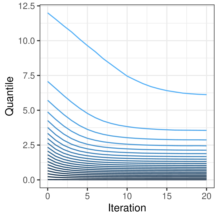
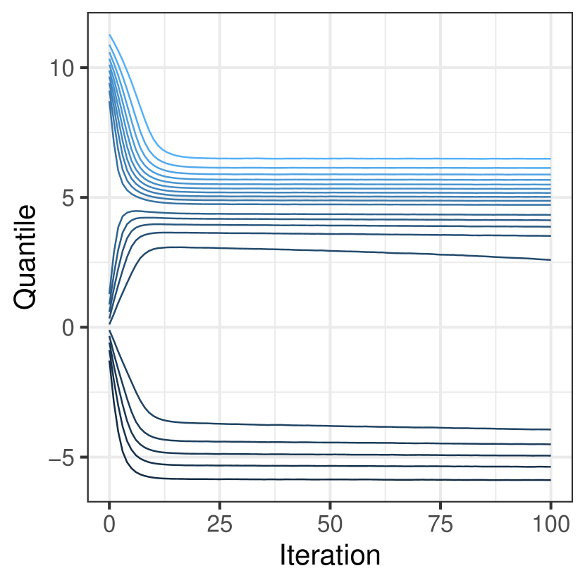
Refer to caption
Refer to caption
Figure 9: Quantiles of (left) the radial component of πtsubscript𝜋𝑡\pi_{t}, and (right) πtsubscript𝜋𝑡\pi_{t}, against iteration t0𝑡0t\geq 0, from probability 0.005 (dark blue) to 0.995 (light blue). The RWM algorithm (left) targeted the logistic target π(x)exp(x)/{1+exp(x)}2proportional-to𝜋𝑥𝑥superscript1𝑥2\pi(x)\propto\exp(x)/\{1+\exp(x)\}^{2} with starting density π0(x)π(x/2)proportional-tosubscript𝜋0𝑥𝜋𝑥2\pi_{0}(x)\propto\pi(x/2), and (left) targeted π=0.5𝒩1(5,1)+0.5𝒩1(5,1)𝜋0.5subscript𝒩1510.5subscript𝒩151\pi=0.5\mathcal{N}_{1}(-5,1)+0.5\mathcal{N}_{1}(5,1) with π0=0.5𝒩1(0,1)+0.5𝒩1(10,1)subscript𝜋00.5subscript𝒩1010.5subscript𝒩1101\pi_{0}=0.5\mathcal{N}_{1}(0,1)+0.5\mathcal{N}_{1}(10,1) and h=22h=2. The condition πtcotπsubscript𝜋𝑡cotsubscript𝜋\pi_{t}\smash{\overset{\vphantom{a}\smash{\textup{cot}}}{\rightsquigarrow}}\pi_{\infty} holds for all t0𝑡0t\geq 0 in the left plot, but fails for t>0𝑡0t>0 in the right plot.

E.3 Gibbs sampler

A thinning factor of 5 was used for both the empirical and the coupling bounds. For the empirical bound, T=5000𝑇5000T=5000 was set, at which point the chain has been stationary for a substantial amount of iterations. The empirical bounds were debiased by averaging in the asymptote for T𝒜={2000,2005,,4000}superscript𝑇𝒜200020054000T^{\prime}\in\mathcal{A}=\{2000,2005,\dots,4000\}. The reflection-maximal coupling (bou-rabee2020coupling; jacob2020unbiased) was used, coordinate-wise, to compute the coupling bound at a lag of L=5000𝐿5000L=5000. With this large value of L𝐿L, all meetings occured before time L𝐿L as measured at the Y𝑌Y-chain, and the coupling bound incurred virtually no loss due to the triangle inequality.

E.3.1 Explanation for the tightness of the bound U𝑈U

The reason why the bound U𝑈U closely follows the true squared Wasserstein distance is due to the essentially low-dimensional nature of the problem, as we now explain. The high correlation in the AR(1) process causes the largest principal components of the target to overshadow the rest (the sum of the five largest eigenvalues is over 90% of the trace), and causes the sampler to explore more easily in the direction of the smallest principal components than in the direction of the larger ones. For all but the earliest few iterations t𝑡t, the marginals πtsubscript𝜋𝑡\pi_{t} of the Gibbs sampler approximately lie in the same low-dimensional subspace, spanned by, say, the five largest principal components of the target π𝜋\pi. When the distributions are approximately supported in a low-dimensional subset of dsuperscript𝑑\mathbb{R}^{d}, the empirical Wasserstein distance has been shown to converge faster than the canonical rate n1/dsuperscript𝑛1𝑑n^{-1/d} for low-to-moderate sample sizes n𝑛n (weed2019sharp, Section 5.3). A faster rate therefore applies to our upper bound U𝑈U as well. This rate, in conjunction with the debiasing term present in U𝑈U, causes the estimator to have a very small bias at the sample size we consider.

E.4 Dimensional scaling of ULA and MALA

The target π=𝒩d(0,Σ)𝜋subscript𝒩𝑑0Σ\pi=\mathcal{N}_{d}(0,\Sigma) with Σij=0.5|ij|subscriptΣ𝑖𝑗superscript0.5𝑖𝑗\Sigma_{ij}=0.5^{|i-j|} corresponds to a d𝑑d-dimensional AR(1)𝐴𝑅1AR(1) process with correlation ρ=0.5𝜌0.5\rho=0.5 and unit noise. Properties of such matrices ΣΣ\Sigma are listed in trench1999asymptotic. The precision matrix Σ1superscriptΣ1\Sigma^{-1} is tridiagonal with a simple closed form, leading to faster gradient computation. The eigenvalues of ΣΣ\Sigma fall between 1/3131/3 and 333, the covariance therefore satisfies Id/3Σ3Idprecedes-or-equalssubscript𝐼𝑑3Σprecedes-or-equals3subscript𝐼𝑑I_{d}/3\preceq\Sigma\preceq 3I_{d} and so is well-conditioned with a condition number of 999. By Proposition 2, it follows that 𝒩d(0,3Id)=π0cotπ=𝒩d(0,Σ)subscript𝒩𝑑03subscript𝐼𝑑subscript𝜋0cot𝜋subscript𝒩𝑑0Σ\mathcal{N}_{d}(0,3I_{d})=\pi_{0}\overset{\vphantom{a}\smash{\textup{cot}}}{\rightsquigarrow}\pi=\mathcal{N}_{d}(0,\Sigma), and so the start π0subscript𝜋0\pi_{0} is appropriately overdispersed with respect to the target π𝜋\pi. The dimension was set to d{50,100,200,300,400,500,600,800,1000}𝑑501002003004005006008001000d\in\{50,100,200,300,400,500,600,800,1000\}.

For MALA, no thinning was used, and the empirical bounds were computed with T=2000𝑇2000T=2000 and debiased by averaging in the asymptote for T𝒜={250,251,,500}superscript𝑇𝒜250251500T^{\prime}\in\mathcal{A}=\{250,251,\dots,500\}. For ULA, the empirical bounds used a thinning factor of 40, and the empirical bounds were computed with T=70000𝑇70000T=70000 and debiased by averaging in the asymptote for T𝒜={8000,8040,,60000}superscript𝑇𝒜8000804060000T^{\prime}\in\mathcal{A}=\{8000,8040,\dots,60000\}. No thinning was used for the coupling bound, and both algorithms used the reflection-maximal coupling (bou-rabee2020coupling; jacob2020unbiased), with a lag of L=2000𝐿2000L=2000 for MALA and a lag of L=70000𝐿70000L=70000 for ULA. With these large values of L𝐿L, all meetings occured before time L𝐿L as measured at the Y𝑌Y-chain. Relative to MALA, the much larger choice of the lag L𝐿L for ULA is due to the much slower mixing of this algorithm. The gap between the debiasing interval 𝒜𝒜\mathcal{A} and the endpoint T𝑇T was chosen significantly larger, in terms of relative size, for MALA than for ULA. This is purely due to the convenience of selecting T=L𝑇𝐿T=L in our simulations, and we emphasize that the bound for MALA exhibits similar performance for smaller values of T𝑇T as well.

Letting TV denote the total variation distance, for parity with the TV(πt,π)0.25TVsubscript𝜋𝑡subscript𝜋0.25\textup{TV}(\pi_{t},\pi_{\infty})\leq 0.25 threshold used in biswas2019estimating mixing times were computed at the threshold 𝒲22(πt,π)6superscriptsubscript𝒲22subscript𝜋𝑡subscript𝜋6\mathcal{W}_{2}^{2}(\pi_{t},\pi_{\infty})\leq 6, because at these thresholds the coupling bounds for both the Wasserstein and the total variation distances indicated similar mixing times.

We remark that for the larger values of d𝑑d we consider, the stationary distribution of ULA does not strictly satisfy π0cotπsubscript𝜋0cotsubscript𝜋\pi_{0}\overset{\vphantom{a}\smash{\textup{cot}}}{\rightsquigarrow}\pi_{\infty}, since we have seen numerically that 3IdΣ3subscript𝐼𝑑subscriptΣ3I_{d}-\Sigma_{\infty} has one negative eigenvalue. However, the absolute value of the negative eigenvalue is invariably negligibly small compared to the others, and so π0cotπsubscript𝜋0cotsubscript𝜋\pi_{0}\overset{\vphantom{a}\smash{\textup{cot}}}{\rightsquigarrow}\pi_{\infty} is approximately satisfied. Our numerical results in Figure 6 confirm that our bounds are robust to this slight discrepancy.

E.4.1 Stationary bias of ULA

By Proposition 5, ULA has a stationary distribution π=𝒩d(0,Σ)subscript𝜋subscript𝒩𝑑0subscriptΣ\pi_{\infty}=\mathcal{N}_{d}(0,\Sigma_{\infty}) with ΣΣsucceeds-or-equalssubscriptΣΣ\Sigma_{\infty}\succeq\Sigma. By Proposition 2 it follows that πcotπsubscript𝜋cot𝜋\pi_{\infty}\smash{\overset{\vphantom{a}\smash{\textup{cot}}}{\rightsquigarrow}}\pi, hence the stationary distribution of ULA is overdispersed with respect to its intended target. Theorem 1 thus enables us to directly quantify the bias of ULA due to its discretization error by an upper bound on 𝒲22(π,π)superscriptsubscript𝒲22𝜋subscript𝜋\mathcal{W}_{2}^{2}(\pi,\pi_{\infty}), which is complemented by the lower bound on 𝒲2(π,π)subscript𝒲2𝜋subscript𝜋\mathcal{W}_{2}(\pi,\pi_{\infty}) from Theorem 2. Bringing these bounds to the same scale, Figure 10 displays the estimators U𝑈U and Lsqsubscript𝐿sqL_{\textup{sq}} for an ULA with step size h=d1/6superscript𝑑16h=d^{-1/6}. The bounds are able to detect the stationary bias of ULA at this step size.
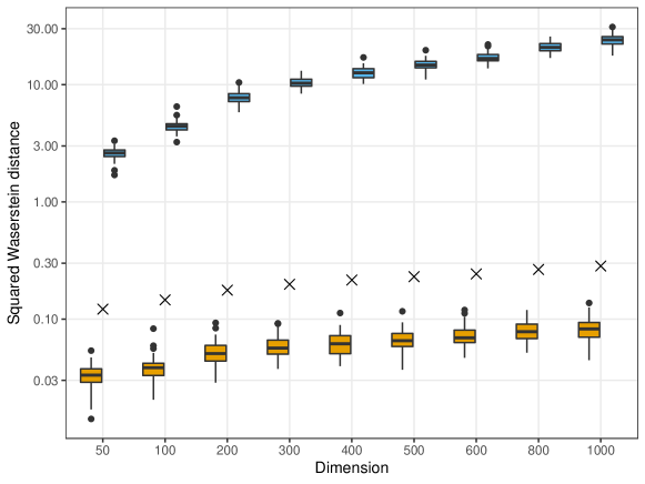
Refer to caption
Figure 10: Estimated bounds on 𝒲22(π,π)superscriptsubscript𝒲22subscript𝜋𝜋\mathcal{W}_{2}^{2}(\pi_{\infty},\pi) for the ULA of Section 4.4.2 with a larger step size h=d1/6superscript𝑑16h=d^{-1/6}. Box plots of 50 estimators U𝑈U ( ) and Lsqsubscript𝐿sqL_{\textup{sq}} ( ) at sample size n=1000𝑛1000n=1000, and exact squared distance ( ). The y𝑦y-axis is on a log10subscript10\log_{10}-scale.

E.4.2 Erratum for biswas2019estimating

We note that our numerical results for the ULA vs MALA scaling are markedly different to those in biswas2019estimating. While our choice of different step sizes and initial distribution are contributing factors, the discrepancy is largely due to an unfortunate error in the code associated to biswas2019estimating, as confirmed by the authors. As opposed to the intended scaling hd1/6similar-tosuperscript𝑑16h\sim d^{-1/6}, both ULA and MALA are instead scaled with a much larger hd1/12similar-tosuperscript𝑑112h\sim d^{-1/12}. This leads to vanishingly small acceptance probabilities for MALA as the dimension is increased. Compared to MALA, ULA does not have an acceptance step. Therefore, in large enough dimension, it converges to its stationary distribution faster than MALA, despite having a step size which was chosen to be a constant factor smaller. At the same time, the larger scaling causes ULA to converge to a stationary distribution which is substantially different from the intended target.

E.5 Stochastic volatility model

The stochastic volatility model we consider echoes (liu2001monte, Section 9.6.2) and (girolami2011riemann, Section 8):

Yt=βεtexp(Xt/2),εt𝒩(0,1),for t=1,,T,formulae-sequencesubscript𝑌𝑡𝛽subscript𝜀𝑡subscript𝑋𝑡2formulae-sequencesimilar-tosubscript𝜀𝑡𝒩01for 𝑡1𝑇\displaystyle Y_{t}=\beta\varepsilon_{t}\exp\left(X_{t}/2\right),\quad\varepsilon_{t}\sim\mathcal{N}(0,1),\quad\textup{for }t=1,\dots,T,
Xt+1=φXt+ηt+1,ηt+1𝒩(0,σ2),for t=1,,T1,formulae-sequencesubscript𝑋𝑡1𝜑subscript𝑋𝑡subscript𝜂𝑡1formulae-sequencesimilar-tosubscript𝜂𝑡1𝒩0superscript𝜎2for 𝑡1𝑇1\displaystyle X_{t+1}=\varphi X_{t}+\eta_{t+1},\quad\eta_{t+1}\sim\mathcal{N}(0,\sigma^{2}),\quad\textup{for }t=1,\dots,T-1,
X1𝒩(0,σ2/(1φ2)).similar-tosubscript𝑋1𝒩0superscript𝜎21superscript𝜑2\displaystyle X_{1}\sim\mathcal{N}\left(0,\sigma^{2}/(1-\varphi^{2})\right).

Here, X1:T=(X1,,XT)subscript𝑋:1𝑇subscript𝑋1subscript𝑋𝑇X_{1:T}=(X_{1},\dots,X_{T}) is a latent AR(1) process, which drives the variance of the logarithm of the data Y1:T=(Y1,,YT)subscript𝑌:1𝑇subscript𝑌1subscript𝑌𝑇Y_{1:T}=(Y_{1},\dots,Y_{T}). We assume that the parameters β𝛽\beta, φ𝜑\varphi and σ𝜎\sigma are fixed. Having observed the data Y1:Tsubscript𝑌:1𝑇Y_{1:T}, the log-posterior density f(X1:TY1:T)𝑓conditionalsubscript𝑋:1𝑇subscript𝑌:1𝑇f(X_{1:T}\mid Y_{1:T}) is, up to a constant offset,

f(X1:TY1:T)=12(t=1TXt+1β2t=1TYt2exp(Xt)+1σ2t=1T1(φXtXt+1)2+1φ2σ2X12).𝑓conditionalsubscript𝑋:1𝑇subscript𝑌:1𝑇12superscriptsubscript𝑡1𝑇subscript𝑋𝑡1superscript𝛽2superscriptsubscript𝑡1𝑇superscriptsubscript𝑌𝑡2subscript𝑋𝑡1superscript𝜎2superscriptsubscript𝑡1𝑇1superscript𝜑subscript𝑋𝑡subscript𝑋𝑡121superscript𝜑2superscript𝜎2superscriptsubscript𝑋12f(X_{1:T}\mid Y_{1:T})=-\frac{1}{2}\left(\sum_{t=1}^{T}X_{t}+\frac{1}{\beta^{2}}\sum_{t=1}^{T}Y_{t}^{2}\exp(-X_{t})+\frac{1}{\sigma^{2}}\sum_{t=1}^{T-1}(\varphi X_{t}-X_{t+1})^{2}+\frac{1-\varphi^{2}}{\sigma^{2}}X_{1}^{2}\right).

The gradient of the log-posterior f𝑓f thus has components

fX1𝑓subscript𝑋1\displaystyle\frac{\partial f}{\partial X_{1}} =12β2Y12exp(X1)φσ2(φX1X2)1φ2σ2X1,absent12superscript𝛽2superscriptsubscript𝑌12subscript𝑋1𝜑superscript𝜎2𝜑subscript𝑋1subscript𝑋21superscript𝜑2superscript𝜎2subscript𝑋1\displaystyle=\frac{1}{2\beta^{2}}Y_{1}^{2}\exp(-X_{1})-\frac{\varphi}{\sigma^{2}}(\varphi X_{1}-X_{2})-\frac{1-\varphi^{2}}{\sigma^{2}}X_{1},
fXt𝑓subscript𝑋𝑡\displaystyle\frac{\partial f}{\partial X_{t}} =12β2Yt2exp(Xt)φσ2(φXtXt+1)1σ2(XtφXt1),for t=2,T1,formulae-sequenceabsent12superscript𝛽2superscriptsubscript𝑌𝑡2subscript𝑋𝑡𝜑superscript𝜎2𝜑subscript𝑋𝑡subscript𝑋𝑡11superscript𝜎2subscript𝑋𝑡𝜑subscript𝑋𝑡1for 𝑡2𝑇1\displaystyle=\frac{1}{2\beta^{2}}Y_{t}^{2}\exp(-X_{t})-\frac{\varphi}{\sigma^{2}}(\varphi X_{t}-X_{t+1})-\frac{1}{\sigma^{2}}(X_{t}-\varphi X_{t-1}),\quad\textup{for }t=2,\dots T-1,
fXT𝑓subscript𝑋𝑇\displaystyle\frac{\partial f}{\partial X_{T}} =12β2YT2exp(XT)1σ2(XTφXT1).absent12superscript𝛽2superscriptsubscript𝑌𝑇2subscript𝑋𝑇1superscript𝜎2subscript𝑋𝑇𝜑subscript𝑋𝑇1\displaystyle=\frac{1}{2\beta^{2}}Y_{T}^{2}\exp(-X_{T})-\frac{1}{\sigma^{2}}(X_{T}-\varphi X_{T-1}).

When using a gradient-based Metropolis-Hastings algorithm, we evaluate the log-posterior and its gradient at proposal X1:Tsubscript𝑋:1𝑇X_{1:T}. We can reduce the total computation time of these steps, perhaps at the expense of additional memory usage. With all operations applied component-wise, we compute the vectors exp(X1:T)subscript𝑋:1𝑇\exp(-X_{1:T}) and φX1:T1X2:T𝜑subscript𝑋:1𝑇1subscript𝑋:2𝑇\varphi X_{1:T-1}-X_{2:T} exactly once, then re-use them for both the posterior and gradient calculation.

The dimension of the problem was T=360𝑇360T=360, equivalent to approximately one year of daily data. Following girolami2011riemann, the parameter values were fixed at β=0.65𝛽0.65\beta=0.65, φ=0.98𝜑0.98\varphi=0.98 and σ=0.15𝜎0.15\sigma=0.15. The data Y1:Tsubscript𝑌:1𝑇Y_{1:T} were simulated from the model.

The MALA was run with a step-size of h=0.13T1/60.13superscript𝑇16h=0.13T^{-1/6}, giving an acceptance rate of around 56%percent5656\%, which is known to be approximately optimal in certain high-dimensional settings (roberts1998optimal). A thinning factor of 505050 was used for both the empirical and coupling bounds. The empirical bounds used T=60000𝑇60000T=60000, and employed debiasing by averaging in the asymptote for T𝒜={20000,20050,,50000}superscript𝑇𝒜200002005050000T^{\prime}\in\mathcal{A}=\{20000,20050,\dots,50000\}. The coupling bound used the reflection-maximal coupling (bou-rabee2020coupling; jacob2020unbiased) with a lag of L=60000𝐿60000L=60000. With this large value of L𝐿L, all meetings occured before time L𝐿L as measured at the Y𝑌Y-chain, and the coupling bound incurred virtually no loss due to the triangle inequality.

The RWM was first run with a step size of h=0.25T1/20.25superscript𝑇12h=0.25T^{-1/2}, for an acceptance rate of around 24%percent2424\%, which is known to be approximately optimal in certain high-dimensional settings (roberts1997weak). A thinning factor of 200020002000 was used for both the empirical and coupling bounds. The empirical bounds used T=3000000𝑇3000000T=3000000 (two orders of magnitude larger than for the MALA), and employed debiasing by averaging in the asymptote for T𝒜={1000000,1002000,,2000000}superscript𝑇𝒜100000010020002000000T^{\prime}\in\mathcal{A}=\{1000000,1002000,\dots,2000000\}. No coupling was used, as all preliminary runs with the reflection-maximal coupling failed to meet within iteration counts two orders of magnitude larger than those considered for the empirical bound. The RWM was then run with a smaller scaling of h=0.1T1/20.1superscript𝑇12h=0.1T^{-1/2}, for an acceptance rate of around 64%percent6464\%. A thinning factor of 200020002000 was used for both the empirical and coupling bounds, and the empirical bound was computed similarly to the larger scaling. The coupling bound was computed with the reflection-maximal coupling and a lag of L=2000000𝐿2000000L=2000000. As measured at the Y𝑌Y-chain, many meetings occur after iteration L𝐿L, causing the coupling bound to lose efficiency due to the triangle inequality. In this example, it was computationally infeasible to increase L𝐿L to where the impact of the triangle inequality was negligible for the coupling bound.

E.5.1 The start from the prior distribution is overdispersed

With the same parameters as outlined above, the MALA was also run started from a twice spread-out version of the target. Samples from the target were obtained from iteration T=60000𝑇60000T=60000 of the previous MALA experiment, then were multiplied by a factor of 2, leading to a starting density π0(x)π(x/2)subscript𝜋0𝑥𝜋𝑥2\pi_{0}(x)\approx\pi(x/2) which satisfies π0cotπsubscript𝜋0cot𝜋\pi_{0}\smash{\overset{\vphantom{a}\smash{\textup{cot}}}{\rightsquigarrow}}\pi (the optimal transport map is T(x)=x/2𝑇𝑥𝑥2T(x)=x/2). Figure 11 compares the empirical bounds obtained from this known overdispersed start to those obtained by starting from the prior. While the bounds indicate that the MALA converges slower when started from the prior, the overall shape of the bounds is similar for both starts, suggesting that the start from the prior is suitably overdispersed with respect to the target.
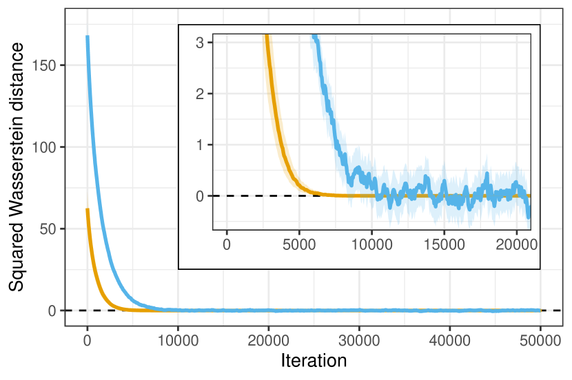
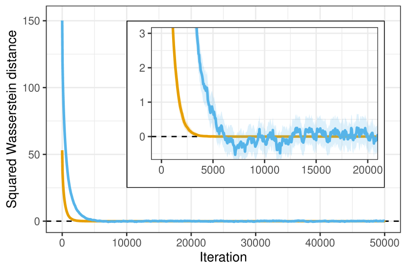
Refer to caption
Refer to caption
Figure 11: Empirical bounds on the squared Wasserstein distance 𝒲22(πt,π)superscriptsubscript𝒲22subscript𝜋𝑡subscript𝜋\mathcal{W}_{2}^{2}(\pi_{t},\pi_{\infty}) ( U𝑈U; Lsqsubscript𝐿sqL_{\textup{sq}}; shaded areas are 95%percent9595\% jackknife confidence intervals) for the MALA targeting the stochastic volatility model. The sampler is started from the prior (left) and a spread-out version of the target (right).

References

  • Biswas et al., (2019) Biswas, N., Jacob, P. E., and Vanetti, P. (2019). Estimating convergence of Markov chains with L-lag couplings. In Advances in Neural Information Processing Systems, volume 32, pages 7391–7401.
  • Boissard and Le Gouic, (2014) Boissard, E. and Le Gouic, T. (2014). On the mean speed of convergence of empirical and occupation measures in Wasserstein distance. Annales de l’Institut Henri Poincaré, Probabilités et Statistiques, 50(2):539–563.
  • Bolley and Villani, (2005) Bolley, F. and Villani, C. (2005). Weighted Csiszár-Kullback-Pinsker inequalities and applications to transportation inequalities. Annales de la Faculté des Sciences de Toulouse, 6, 14(3):331–352.
  • Bonneel et al., (2011) Bonneel, N., van de Panne, M., Paris, S., and Heidrich, W. (2011). Displacement interpolation using Lagrangian mass transport. ACM Transactions on Graphics, 30(6):1–12.
  • Bou-Rabee et al., (2020) Bou-Rabee, N., Eberle, A., and Zimmer, R. (2020). Coupling and convergence for Hamiltonian Monte Carlo. The Annals of Applied Probability, 30(3):1209 – 1250.
  • Brenier, (1991) Brenier, Y. (1991). Polar factorization and monotone rearrangement of vector-valued functions. Communications on Pure and Applied Mathematics, 44(4):375–417.
  • Chizat et al., (2020) Chizat, L., Roussillon, P., Léger, F., Vialard, F.-X., and Peyré, G. (2020). Faster Wasserstein distance estimation with the Sinkhorn divergence. In Advances in Neural Information Processing Systems, volume 33.
  • Crouse, (2016) Crouse, D. F. (2016). On implementing 2d rectangular assignment algorithms. IEEE Transactions on Aerospace and Electronic Systems, 52(4).
  • DasGupta, (2008) DasGupta, A. (2008). Asymptotic theory of statistics and probability. Springer, 1 edition.
  • del Barrio et al., (2021) del Barrio, E., González-Sanz, A., and Loubes, J.-M. (2021). Central limit theorems for general transportation costs. arXiv preprint arXiv:2102.06379.
  • del Barrio and Loubes, (2019) del Barrio, E. and Loubes, J.-M. (2019). Central limit theorems for empirical transportation cost in general dimension. Annals of Probability, 47(2):926–951.
  • Dowson and Landau, (1982) Dowson, D. and Landau, B. (1982). The fréchet distance between multivariate normal distributions. Journal of Multivariate Analysis, 12(3):450–455.
  • Eddelbuettel and Balamuta, (2018) Eddelbuettel, D. and Balamuta, J. J. (2018). Extending R with C++: A brief introduction to Rcpp. The American Statistician, 72(1):28–36.
  • Gelbrich, (1990) Gelbrich, M. (1990). On a formula for the L2 Wasserstein metric between measures on Euclidean and Hilbert spaces. Mathematische Nachrichten, 147(1):185–203.
  • Gilks and Wild, (1992) Gilks, W. R. and Wild, P. (1992). Adaptive Rejection Sampling for Gibbs Sampling. Journal of the Royal Statistical Society: Series C (Applied Statistics), 41(2):337–348.
  • Girolami and Calderhead, (2011) Girolami, M. and Calderhead, B. (2011). Riemann manifold Langevin and Hamiltonian Monte Carlo methods. Journal of the Royal Statistical Society: Series B (Statistical Methodology), 73(2):123–214.
  • Gómez et al., (2003) Gómez, E., A, G.-V. M., and Marín, J. M. (2003). A survey on continuous elliptical vector distributions. Revista Matemática Complutense, 16:345––361.
  • Gozlan and Léonard, (2007) Gozlan, N. and Léonard, C. (2007). A large deviation approach to some transportation cost inequalities. Probability Theory and Related Fields, 139:235–283.
  • Higham, (2008) Higham, N. J. (2008). Functions of Matrices: Theory and Computation. SIAM.
  • Jacob et al., (2020) Jacob, P. E., O’Leary, J., and Atchadé, Y. F. (2020). Unbiased Markov chain Monte Carlo methods with couplings. Journal of the Royal Statistical Society: Series B (Statistical Methodology), 82(3):543–600.
  • Jonker and Volgenant, (1987) Jonker, R. and Volgenant, A. (1987). A shortest augmenting path algorithm for dense and sparse linear assignment problems. Computing, 38(4):325–340.
  • Jonker and Volgenant, (1986) Jonker, R. and Volgenant, T. (1986). Improving the Hungarian assignment algorithm. Operations Research Letters, 5(4):171–175.
  • Kakade et al., (2012) Kakade, S. M., Shalev-Shwartz, S., and Tewari, A. (2012). Regularization techniques for learning with matrices. Journal of Machine Learning Research, 13(59):1865–1890.
  • Kim and Milman, (2012) Kim, Y.-H. and Milman, E. (2012). A generalization of Caffarelli’s contraction theorem via (reverse) heat flow. Mathematische Annalen, 354(3):827–862.
  • Kolesnikov, (2010) Kolesnikov, A. V. (2010). Mass transportation and contractions. Proceedings of the Moscow Institute of Physics and Technology, 2(4):90–99.
  • Liu, (2001) Liu, J. S. (2001). Monte Carlo Strategies in Scientific Computing. Springer.
  • Manole et al., (2021) Manole, T., Balakrishnan, S., Niles-Weed, J., and Wasserman, L. (2021). Plugin estimation of smooth optimal transport maps. arXiv preprint arXiv:2107.12364.
  • McCann, (1995) McCann, R. J. (1995). Existence and uniqueness of monotone measure-preserving maps. Duke Mathematical Journal, 80(2):309–323.
  • McDiarmid, (1989) McDiarmid, C. (1989). On the method of bounded differences. In Siemons, J., editor, Surveys in Combinatorics, 1989: Invited Papers at the Twelfth British Combinatorial Conference, pages 148–188. Cambridge University Press.
  • Nesterov, (2004) Nesterov, Y. (2004). Introductory Lectures on Convex Optimization. Springer.
  • Panaretos and Zemel, (2019) Panaretos, V. M. and Zemel, Y. (2019). Statistical aspects of Wasserstein distances. Annual Review of Statistics and Its Application, 6(1):405–431.
  • Peyré and Cuturi, (2019) Peyré, G. and Cuturi, M. (2019). Computational optimal transport. Foundations and Trends in Machine Learning, 11(5-6):355–607.
  • R Core Team, (2020) R Core Team (2020). R: A Language and Environment for Statistical Computing. R Foundation for Statistical Computing, Vienna, Austria.
  • Roberts et al., (1997) Roberts, G. O., Gelman, A., and Gilks, W. R. (1997). Weak convergence and optimal scaling of random walk Metropolis algorithms. The Annals of Applied Probability, 7(1):110–120.
  • Roberts and Rosenthal, (1998) Roberts, G. O. and Rosenthal, J. S. (1998). Optimal scaling of discrete approximations to Langevin diffusions. Journal of the Royal Statistical Society: Series B (Statistical Methodology), 60(1):255–268.
  • Roberts and Sahu, (1997) Roberts, G. O. and Sahu, S. K. (1997). Updating schemes, correlation structure, blocking and parameterization for the Gibbs sampler. Journal of the Royal Statistical Society: Series B (Statistical Methodology), 59(2):291–317.
  • Sriperumbudur et al., (2012) Sriperumbudur, B. K., Fukumizu, K., Gretton, A., Schölkopf, B., and Lanckriet, G. R. G. (2012). On the empirical estimation of integral probability metrics. Electronic Journal of Statistics, 6:1550–1599.
  • Trench, (1999) Trench, W. F. (1999). Asymptotic distribution of the spectra of a class of generalized Kac–Murdock–Szegö matrices. Linear Algebra and its Applications, 294(1):181–192.
  • Villani, (2009) Villani, C. (2009). Optimal Transport: Old and New. Springer.
  • Weed and Bach, (2019) Weed, J. and Bach, F. (2019). Sharp asymptotic and finite-sample rates of convergence of empirical measures in Wasserstein distance. Bernoulli, 25(4A):2620–2648.
  • Wibisono, (2018) Wibisono, A. (2018). Sampling as optimization in the space of measures: The Langevin dynamics as a composite optimization problem. In Proceedings of the 31st Conference On Learning Theory, volume 75, pages 2093–3027. PMLR.