Rapidly encoding generalizable dynamics in a Euclidean symmetric neural network: a Slinky case study

Abstract

Slinky, a helical elastic rod, is a seemingly simple structure with unusual mechanical behavior; for example, it can walk down a flight of stairs under its own weight. Taking the Slinky as a test-case, we propose a physics-informed deep learning approach for building reduced-order models of physical systems. The approach introduces a Euclidean symmetric neural network (ESNN) architecture that is trained under the neural ordinary differential equation framework to learn the 2D latent dynamics from the motion trajectory of a reduced-order representation of the 3D Slinky. The ESNN implements a physics-guided architecture that simultaneously preserves energy invariance and force equivariance on Euclidean transformations of the input, including translation, rotation, and reflection. The embedded Euclidean symmetry provides physics-guided interpretability and generalizability, while preserving the full expressive power of the neural network. We demonstrate that the ESNN approach is able to accelerate simulation by one to two orders of magnitude compared to traditional numerical methods and achieve a superior generalization performance, i.e., the neural network, trained on a single demonstration case, predicts accurately on unseen cases with different Slinky configurations and boundary conditions.

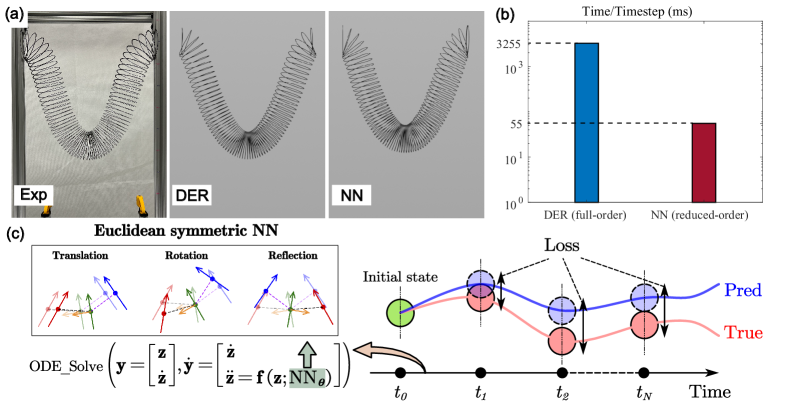
Figure 1: (color online). (a) Static deformation comparison across a real-world Slinky experiment, the discrete elastic rod (DER) simulation, and the reduced-order model based on the Euclidean symmetric neural network. (b) Computation time comparison between DER simulation and the proposed NN method. (c) The core features of the proposed NN method: the NN embeds energy invariance and force equivariance on Euclidean transformations of the input Slinky configuration, including translation, rotation, and reflection. The NN is trained under the neural ordinary differential equation framework.

Many dynamical systems are computationally expensive to simulate with classic numerical methods based on discretized differential equations, due to the fine spatiotemporal resolution required for the discretization to hold. More efficient yet effective dynamics predictions are widely demonstrated by humans. The high efficiency is largely due to their ability to make predictions at coarser resolution levels, sometimes for only perceivable states. Such simplification is similar to reduced-order modeling [1, 2, 3, 4] with a cognitive mapping from actual states to reduced (latent) states. The reduced-order dynamics describing the reduced degrees of freedom (DoFs) will consequently differ from first principles in physics, and need to be learned from observations with data-driven approaches. An important tool that incorporates data-driven methods to augment physics models is deep learning [5] based on deep neural networks (DNNs), universal approximators that show excellent data-fitting power. On one hand, the data-driven models offer possibilities for superior computation efficiency compared to classic methods [6, 7, 8]; e.g., as demonstrated in this Letter, the computation time can be cut down by one to two orders of magnitude. On the other hand, it enables advances towards human-like, automated rule discovery and learning of the dynamics of a system from observations [9, 10, 11, 12, 13, 14].

Unconstrained neural networks (NNs), trained to directly fit time-series data generated by dynamical systems, however, often cannot replicate dynamics under unseen initial and boundary conditions because they fail to learn the underlying physics-constraints, such as Euclidean symmetry of space and conservation of energy. Indeed, recent works have shown that incorporating such constraints into deep learning is vital for generalization ability, learning efficiency, and interpretability [15, 16]. For example, Hamiltonian Neural Network [17] and Lagrangian Neural Network [18] introduced the physical prior of energy conservation to neural networks for learning dynamics. Geometric deep learning [16, 19] and equivariant neural networks [20, 21, 22, 23] leverage geometric symmetry properties of the network input to improve the quality of inherent knowledge learned by neural networks. Successful applications include drug discovery [24, 25], quantum chemistry [26], and particle physics [27, 28].

In this Letter, we introduce a physics-informed deep learning approach to learning a 2D reduced-order dynamics of a Slinky. Instead of a long elastic helix in 3D space, a Slinky is described as a series of connected bars in a 2D plane [29]. The approach is guided by two principles: (i) The system trajectories along time are constructed by integrating the ordinary differential equation (ODE) formulated by Newton’s second law of motion; and (ii) A neural network is trained to predict the 2D surrogate forces on the bars so that the observed trajectories can be generated following the ODEs. We endow the neural force predictor with Euclidean symmetry and energy conservation, which combines expressiveness with physics-guided generalizability. In addition, the neural force predictor is faced with the challenge of compounding error, i.e., the error in force prediction at each time step can accumulate, leading to an erroneous simulated trajectory that seriously deviates from reality. We address this by going beyond learning separated state-force pairs, and use the Neural Ordinary Differential Equation (NODE) framework [30] to match the entire trajectory. Under such framework, the consequence of a force prediction error in later time steps is considered in the loss, encouraging the neural network to be prescient and not to overfit proximate dynamics.

We show that this approach can accurately predict the motion of a real-world Slinky using 2D reduced-order representation of the Slinky. This approach is able to generalize to unseen Slinky configurations and boundary conditions by learning from a single demonstration case. The computational speed is increased by roughly 60 times compared to the traditional 3D modelling technique due to the significantly reduced DoFs, in spite of the relatively more complicated latent dynamics (Fig. 1). Moreover, the approach can generalize by exploiting “physics” – the neural force vector can be scaled with the material stiffness to predict the motion of a softer (previously unseen) Slinky. To the best of the authors’ knowledge, we for the first time demonstrate, with experimental validation, that a deep learning approach is capable of extensively generalizing from one single learning case, and that a complex system in the real world could benefit from this reality-virtual-reality closed-loop pipeline.

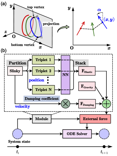
Figure 2: (color online). (a) Construction of the 2D bars by projecting 3D Slinky cycles into the XOY plane. Each 2D bar has 3 DoFs: $x$ and $y$ at its center, and the angle $\alpha$ with respect to the $y$-axis. (b). Time marching under the NODE framework. For the system at time $t_{i}$, the Slinky system is partitioned into triplets (3 adjacent bars) and passed through the same ESNN. The output vectors are stacked as the elastic force vector for the Slinky system. The total external force vector is the summation of elastic, gravity, and damping force vectors. The total external force and the system state at $t_{i}$ are fed into an ODE solver to update the system state at $t_{i+1}$.

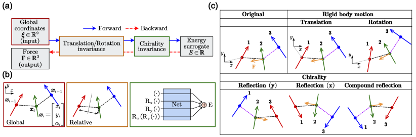
Figure 3: (color online). (a) Workflow of the ESNN. The ESNN takes the global coordinates of a triplet as input, and generates the surrogate elastic force on the middle bar of the triplet as output. The ESNN first removes the rigid body DoFs from the input and then applies a chirality invariance module. An energy surrogate is calculated, which is invariant to rigid body and chiral transformations of the input. The output of the NN is computed by taking the derivative of the energy surrogate with respect to the coordinates of the middle bar in the input. The output is equivariant to rigid body and chiral transformations of the input. (b) Visualization of the input, rigid body motion removal, chiral transformation modules. The Net in the chiral transformation module is a DenseNet-like neural network of 5 hidden layers. For detailed neural network construction, refer to [31]. (c) Summary of the energy invariance and force equivariance properties of the ESNN. The original triplet configuration and its Euclidean transformed copies generate the same energy surrogate (invariance) and equivariant force vectors.

Given 3D Slinky motion data at a series of time steps, we first construct the 2D data as the ground truth for NN training. As shown in Fig. 2(a), the top and bottom vertices of each Slinky cycle are projected onto the XOY plane. The vector pointing from the projected bottom vertex to the projected top vertex of a cycle is the 2D representation of that cycle, referred to as a bar in the following. The coordinates of the $i$th bar are $\mathbf{x}_{i}=[x_{i},y_{i},\alpha_{i}]\in\mathbb{R}^{3}$: $x_{i}$ and $y_{i}$ are the coordinates of the center point, and $\alpha_{i}$ is the angle with respect to the $y$ axis. Three adjacent bars group into a triplet with 9 coordinates. The surrogate elastic force on the middle bar of a triplet will be completely determined by these 9 coordinates. For a Slinky of $N_{c}$ cycles, its 2D representation has $N_{c}$ bars and $N_{c}$ triplets ($N_{c}$ instead of $N_{c}$-2 because of special boundary treatment), and the states of these $N_{c}$ bars at different time steps constitute the 2D system trajectory of the Slinky. Such a 2D reduced-order representation retains the essential geometry of the 3D structure of a Slinky, based on which a 3D helical shape is still reconstructable despite the substantial reduction in the number of DoFs. This property guarantees the reliable estimation of the elastic potential using 2D reduced-order states. See SM [31] for boundary condition treatment and reconstruction of 3D Slinky shapes. After acquiring the 2D system trajectory, the reduced-order dynamics is learned by an ESNN under the NODE framework.

Fig. 3 shows the workflow of the ESNN. The input of the NN is the global coordinates of a triplet $\bm{\mathrm{\xi}}=[\mathbf{x}_{i-1}^{T},\mathbf{x}_{i}^{T},\mathbf{x}_{i+1}^{T}]^{T}\in\mathbb{R}^{9}$, where $\mathbf{x}_{i}\in\mathbb{R}^{3}$ is the coordinates of the $i$th bar and the superscript $T$ represents transpose operation. The first step in the ESNN is to make the representation invariant with respect to rigid body translation and rotation. This is accomplished by transforming the global coordinates $\bm{\mathrm{\xi}}$ into the relative coordinates $\mathbf{z}\in\mathbb{R}^{6}$. Then $\mathbf{z}$ and its 3 reflected copies are passed through a DenseNet-like structure [32] parameterized by $\bm{\theta}$, denoted as $f_{\bm{\theta}}(\cdot)$. The outputs are 4 scalars, and their summation is the energy surrogate $E$:

$$\begin{split}E(\mathbf{z})=f_{\bm{\theta}}&(\mathbf{z})+f_{\bm{\theta}}(R_{x}(\mathbf{z}))+\\ &f_{\bm{\theta}}(R_{y}(\mathbf{z}))+f_{\bm{\theta}}(R_{x}(R_{y}(\mathbf{z}))),\end{split}$$ (1)

where $R_{x}(\cdot)$ and $R_{y}(\cdot)$ stand for the reflection of the triplet coordinates about $x$ and $y$ axes. Note that the reflections are self-inverse and commutative, i.e.,

$$R_{x}(R_{x}(\cdot)) =I(\cdot),\quad R_{y}(R_{y}(\cdot))=I(\cdot),~{}\textrm{and}$$

$$R_{x}(R_{y}(\cdot)) =R_{y}(R_{x}(\cdot)),$$

where $I(\cdot)$ is the identity transformation. Therefore, the energy surrogate $E$ satisfies the following property:

$$E(\mathbf{z})=E(R_{x}(\mathbf{z}))=E(R_{y}(\mathbf{z}))=E(R_{x}(R_{y}(\mathbf{z}))).$$ (2)

That is, $E$ is invariant to reflections on $\mathbf{z}$ and thus on $\bm{\mathrm{\xi}}$; $E$ is also invariant to rigid body transformation on $\bm{\mathrm{\xi}}$ due to such invariance of $\mathbf{z}$. The output surrogate force vector $\mathbf{F}\in\mathbb{R}^{3}$ is generated by taking the derivative of $E$ with respect to $\mathbf{x}_{i}\in\mathbb{R}^{3}$ using the automatic differentiation mechanism in PyTorch [33], i.e., $\mathbf{F}=\mathbf{F}(\bm{\mathrm{\xi}})=\mathrm{\partial}E(\bm{\mathrm{\xi}})/\mathrm{\partial}\mathbf{x}_{i}$. It is straightforward to prove that $\mathbf{F}$ is equivariant to rigid body and chiral transformation on $\bm{\mathrm{\xi}}$, i.e., denoting translation, rotation, and reflection on $\bm{\mathrm{\xi}}$ as $T(\bm{\mathrm{\xi}})$, $Ro(\bm{\mathrm{\xi}})$, and $Rf(\bm{\mathrm{\xi}})$, we have $\mathbf{F}(T(\bm{\mathrm{\xi}}))=\mathbf{F}(\bm{\mathrm{\xi}})$, $\mathbf{F}(Ro(\bm{\mathrm{\xi}}))=Ro(\mathbf{F}(\bm{\mathrm{\xi}}))$, and $\mathbf{F}(Rf(\bm{\mathrm{\xi}}))=Rf(\mathbf{F}(\bm{\mathrm{\xi}}))$.

The entire ESNN can be considered as a general function $\mathbf{F}=\mathrm{ESNN}_{\bm{\theta}}(\bm{\mathrm{\xi}})$, while the aforementioned invariances / equivariances are guaranteed regardless of the parameters $\bm{\theta}$. Conventionally, to obtain a good performance with an unconstrained neural network for all orientation / chirality of the input, the approach is to augment the training dataset with various rotation and reflection. In comparison, the advantages of ESNN are trifold: (1) The Euclidean symmetry is strictly guaranteed (instead of only approximated in the dataset-augmentation approach); (2) Training cost is significantly lower due to the concise training dataset without symmetry augmentation; (3) A compact NN architecture is possible since weights are dedicated to learn the functional form of the surrogate elastic energy instead of the symmetries. This bolsters the succeeding gain in computational speed. The entire workflow and the invariance / equivariance properties are illustrated in Fig. 3.

Fig. 2(b) shows the schematic of the 2D reduced-order dynamics in our framework, specifically, how a 2D state is evolved from time $t_{i}$ to time $t_{i+1}$. At each time step, we first construct $N_{c}$ triplets and pass them through the ESNN. The output will be $N_{c}$ 3-dimensional vectors representing the predicted surrogate elastic forces on the middle bars of the triplets. These vectors are then concatenated to form the elastic force vector for the entire Slinky system. The summation of this elastic force vector, the gravity force vector, and the damping force vector is the total external force vector of the Slinky system. Then the system state can be updated by any ODE solver, 5th order Dormand–Prince method in this Letter. By repeating this update procedure from a known initial state, a predicted trajectory for the reduced-order Slinky system is calculated. The ESNN weights $\bm{\theta}$ will be trained on the loss comparing the ground truth trajectory and the predicted one (Fig. 1(c)). This NODE training scheme enables accuracy and stability: the ESNN should not only predict surrogate forces accurately but also accurately in the way that after passing the predicted forces through an ODE solver, the errors in the calculated trajectories do not compound.

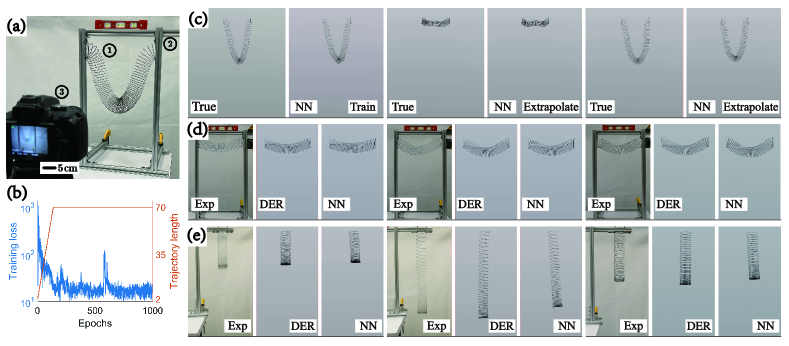
Figure 4: (color online). (a) Experimental apparatus: a 76-cycle Slinky is supported by an experiment frame . A camera records the Slinky motion. (b) The loss history of the NODE training for 1000 epochs. The training trajectory length is gradually increased from 2 to 70. (c) Comparison between 3D DER ground truth and reconstruction from the ESNN reduced-order model in train phase and extrapolation phase. Time shots are at 0.45 s, 2.03 s, and 2.50 s (from left to right). (d) Comparison across real-world Slinky experiment, 3D DER simulation, and reconstruction from the ESNN reduced-order model. Testing is performed on a 40-cycle Slinky, unseen by the ESNN. Time shots are at 0.53 s, 1.43 s, and static (from left to right). (e) Comparison of testing on a 40-cycle Slinky with a different boundary condition and orientation from the training case. Time shots are at 0.2 s, 0.53 s, and static (from left to right).

We test the ESNN on a commercially-available 76-cycle Slinky (Poof-Slinky, Inc.). The experiment setup is shown in Fig. 4(a). We record a single Slinky motion case using a camera, then calibrate a 3D discrete elastic rod (DER) model [34, 35, 36, 37, 38] for comparison and generation of 2D training data, and then train the ESNN on the 2D data of this single case. After training, we freeze the NN model and test its generalization ability across several unseen cases.

First we measure the geometry and mass of the 76-cycle Slinky. Then a motion video is captured with its both ends clamped to the frame. The Slinky is initially held horizontal and dropped freely under gravity. A 3D DER model of the Slinky is built with the same geometry and mass. The Young’s modulus and the damping parameter are calibrated to match the DER-generated Slinky motion with the video-recorded one. A 3D simulation is generated based on the calibrated model with the same initial and boundary conditions as the experiment and with the damping removed. The 2D system trajectory will be constructed based on projection of the generated 3D data and used to train an ESNN. The ESNN will be frozen after training. A damping and a contact model [39] will be added in the NN deployment to match the real-world energy dissipation and non-penetration. The ESNN is trained on this one case, and tested for other cases with different boundary conditions, Slinky orientation, and number of cycles. For parameter calibration details, please refer to [31].

When the ESNN is randomly initialized, a long trajectory prediction will consume too much ODE solution time. A better strategy is to make short trajectory predictions initially, update the ESNN weights, and then gradually increase the learning trajectory length. We start with trajectory length of 2 and increase the length by 1 every 2 epochs until it reaches 70. After that the trajectory length stays the same. The simulation time step is 0.01 s. So eventually the ESNN is trained on a ground truth trajectory of 0.7 s. In each epoch, the states of 20 randomly selected bars are used in the loss function:

$$loss=\sum_{t_{k}}\sum_{i=1}^{20}\|\mathbf{W}(\mathbf{x}_{s_{i}}^{(k)}-\hat{\mathbf{x}}_{s_{i}}^{(k)})\|_{2}^{2}+\|\mathbf{W}(\mathbf{v}_{s_{i}}^{(k)}-\hat{\mathbf{v}}_{s_{i}}^{(k)})\|_{2}^{2}$$ (3)

where $\mathbf{W}\in\mathbb{R}^{3\times 3}$ is a weight matrix, $s_{i}$ is the index of the $i$th randomly selected bar, $\mathbf{x}_{s_{i}}^{(k)}$ and $\mathbf{v}_{s_{i}}^{(k)}$ are the ground truth position and velocity of the $i$th randomly selected bar at time $t_{k}$, $\hat{\mathbf{x}}_{s_{i}}^{(k)}$ and $\hat{\mathbf{v}}_{s_{i}}^{(k)}$ are the corresponding predications. The training loss history and trajectory length are shown in Fig 4(b).

After 1000 training epochs, a simulation is run with the trained ESNN for 2.5 s. The predicted trajectory, of which the first 0.7 s span is called train phase and the 0.7 - 2.5 s span extrapolation phase, is compared with 3D DER simulation in Fig. 4(c). The ESNN results not only match the ground truth well within the train phase, but also perform well in the extrapolation phase up to 2.5 s, i.e., more than 2 times the training time span. The final static deformations for experiment, DER, and ESNN are in good agreement, as shown in Fig. 1(a). The computation times of one-second-long simulations for DER and ESNN are compared in Fig. 1(b). ESNN outperforms the traditional DER method by roughly 60 times due to the significant reduction in the number of DoFs. With the ESNN weights and all physical parameters for both DER and NN fixed, we test the generalization of the ESNN on previously unseen cases: on a Slinky (1) of a different number of cycles; (2) under a different boundary condition; (3) of a different density; (4) of a different Young’s modulus (refer to [31] for (3) and (4)). In the first test case, the Slinky cycle number is changed to 40 with both ends clamped to the frame, as shown in Fig. 4(d). The 40 cycle Slinky is initially held horizontal and then dropped freely under gravity. The dynamic motion at 0.53 s, 1.43 s, and the static deformation of the Slinky from experiment, DER simulation, and ESNN simulation are compared in the Fig. 4(d) and showed an excellent agreement. In the second test case, the 40-cycle Slinky is held vertically, clamped at the upper end, and then dropped freely from its undeformed configuration. The dynamic motion at 0.2 s, 0.53 s, and the static deformation of the Slinky from experiment, DER simulation, and ESNN simulation are compared in the Fig. 4(e) and again we observe a good agreement. In these two test cases, a satisfactory agreement is achieved without making any changes to the ESNN. The agreement originates from the embedded Euclidean symmetry of the NN and the fact that the NN is learning generalizable physics with a local construction. As a contrast, NN methods from [12, 40] construct surrogate models for full-field solutions under a certain boundary condition. The benefit is that the NN prediction is extremely fast since only one forward-pass through the trained NN is required for each prediction. The price paid is in the generalization ability. For a different type of boundary condition, the NNs need to learn from scratch, and a new training dataset dedicated to the new boundary condition is required. However, in our ESNN approach, different boundary conditions can be readily incorporated after trained on a single case since the ESNN focuses on learning local physics which is boundary condition agnostic. In our second test case, the orientation of the Slinky is shifted by 90 degrees. The ESNN is still capable of generating the correct elastic forces and system trajectory prediction since it preserves rotation equivariance.

We have proposed an ESNN-based approach for building data-driven reduced-order models of physical systems under the NODE framework. We have validated its accuracy and extensive generalization ability, a critical differentiation from existing data-driven methods, on real-world Slinky experiments. A roughly 60 times computational acceleration is achieved compared with classic simulation methods. The generalization ability originates from the physics-guided design of the NN architecture, which embeds Euclidean symmetry, including translation, rotation, and chirality invariance for surrogate energy and equivariance for surrogate force. With these features, the ESNN is able to learn the reduced-order physics from a single demonstration case, and perform accurate and accelerated predictions on a variety of unseen cases. By incorporating only a widely applicable geometric symmetry instead of any domain specific knowledge or physical constraints, the ESNN possesses the promise to be universal to a wide variety of physical systems.

We thank Mingjian Lu for his assistance on simulation implementation, and Zhuonan Hao and Dezhong Tong for their assistance on experiments. We are grateful for financial support from the National Science Foundation (NSF) under award number CMMI-2053971. Q.L. and M.K.J are grateful for support from NSF (IIS-1925360). M.K.J is grateful for support from NSF (CAREER-2047663, CMMI-2101751).

See pages ,- of supp_info.pdf

References

- Benner et al. [2017] P. Benner, M. Ohlberger, A. Cohen, and K. Willcox, Model Reduction and Approximation, Computational Science & Engineering (Society for Industrial and Applied Mathematics, 2017).
- Hartman and Mestha [2017] D. Hartman and L. K. Mestha, in 2017 IEEE Conference on Control Technology and Applications (CCTA) (2017) pp. 1917–1922.
- Fulton et al. [2019] L. Fulton, V. Modi, D. Duvenaud, D. I. W. Levin, and A. Jacobson, Computer Graphics Forum 38, 379 (2019).
- Maulik et al. [2020] R. Maulik, A. Mohan, B. Lusch, S. Madireddy, P. Balaprakash, and D. Livescu, Physica D: Nonlinear Phenomena 405, 132368 (2020).
- Karniadakis et al. [2021] G. E. Karniadakis, I. G. Kevrekidis, L. Lu, P. Perdikaris, S. Wang, and L. Yang, Nature Reviews Physics , 1–19 (2021).
- Hezaveh et al. [2017] Y. D. Hezaveh, L. P. Levasseur, and P. J. Marshall, Nature 548, 555 (2017).
- Fournier et al. [2020] R. Fournier, L. Wang, O. V. Yazyev, and Q. Wu, Physical Review Letters 124, 056401 (2020).
- Heiden et al. [2021] E. Heiden, D. Millard, E. Coumans, Y. Sheng, and G. S. Sukhatme, in 2021 IEEE International Conference on Robotics and Automation (ICRA) (2021) pp. 9474–9481.
- Chua et al. [2019] A. J. K. Chua, C. R. Galley, and M. Vallisneri, Physical Review Letters 122, 211101 (2019).
- Rubanova et al. [2019] Y. Rubanova, R. T. Q. Chen, and D. K. Duvenaud, in Advances in Neural Information Processing Systems, Vol. 32 (2019).
- Champion et al. [2019] K. Champion, B. Lusch, J. N. Kutz, and S. L. Brunton, Proceedings of the National Academy of Sciences 116, 22445 (2019).
- Li et al. [2020a] Z. Li, N. B. Kovachki, K. Azizzadenesheli, B. Liu, K. Bhattacharya, A. Stuart, and A. Anandkumar (2020).
- Iten et al. [2020] R. Iten, T. Metger, H. Wilming, L. d. Rio, and R. Renner, Physical Review Letters 124, 010508 (2020).
- Liu and Tegmark [2021] Z. Liu and M. Tegmark, Physical Review Letters 126, 180604 (2021).
- Zhang et al. [2018] P. Zhang, H. Shen, and H. Zhai, Physical Review Letters 120, 066401 (2018).
- Atz et al. [2021] K. Atz, F. Grisoni, and G. Schneider, Nature Machine Intelligence , 1 (2021).
- Greydanus et al. [2019] S. Greydanus, M. Dzamba, and J. Yosinski, in Advances in Neural Information Processing Systems, Vol. 32 (2019).
- Cranmer et al. [2020] M. Cranmer, S. Greydanus, S. Hoyer, P. Battaglia, D. Spergel, and S. Ho, in ICLR 2020 Workshop on Integration of Deep Neural Models and Differential Equations (2020).
- Bronstein et al. [2021] M. M. Bronstein, J. Bruna, T. Cohen, and P. Veličković, arXiv:2104.13478 [cs, stat] (2021).
- Weiler et al. [2018] M. Weiler, M. Geiger, M. Welling, W. Boomsma, and T. Cohen, in Proceedings of the 32nd International Conference on Neural Information Processing Systems (2018) pp. 10402–10413.
- Thomas et al. [2018] N. Thomas, T. Smidt, S. Kearnes, L. Yang, L. Li, K. Kohlhoff, and P. Riley, arXiv:1802.08219 [cs.LG] (2018).
- Finzi et al. [2021] M. Finzi, M. Welling, and A. G. Wilson, arXiv:2104.09459 [cs, math, stat] (2021).
- Satorras et al. [2021] V. G. Satorras, E. Hoogeboom, and M. Welling, arXiv:2102.09844 [cs, stat] (2021).
- Gawehn et al. [2016] E. Gawehn, J. A. Hiss, and G. Schneider, Molecular Informatics 35, 3–14 (2016).
- Jiménez-Luna et al. [2021] J. Jiménez-Luna, F. Grisoni, N. Weskamp, and G. Schneider, Expert Opinion on Drug Discovery 16, 1–11 (2021).
- Gilmer et al. [2017] J. Gilmer, S. S. Schoenholz, P. F. Riley, O. Vinyals, and G. E. Dahl, arXiv (2017).
- Komiske et al. [2019] P. T. Komiske, E. M. Metodiev, and J. Thaler, Journal of High Energy Physics 2019 (2019).
- Qu and Gouskos [2020] H. Qu and L. Gouskos, Physical Review D 101, 056019 (2020).
- Holmes et al. [2014] D. P. Holmes, A. D. Borum, B. F. Moore, R. H. Plaut, and D. A. Dillard, International Journal of Non-Linear Mechanics 65, 236 (2014).
- Chen et al. [2018] R. T. Q. Chen, Y. Rubanova, J. Bettencourt, and D. K. Duvenaud, in Advances in Neural Information Processing Systems, Vol. 31 (2018).
- [31] See supplement material for details on discrete elastic rod simulation, incremental potential contact model, the neural network architecture, special boundary condition treatment of triplets, 3D slinky shape reconstruction, experimental calibration procedure, generalization to different density and elasticity, simulation environment setup, and supplemental movies.
- Huang et al. [2017] G. Huang, Z. Liu, L. Van Der Maaten, and K. Q. Weinberger, in Proceedings of the IEEE Conference on Computer Vision and Pattern Recognition (2017) pp. 4700–4708.
- Paszke et al. [2019] A. Paszke, S. Gross, F. Massa, A. Lerer, J. Bradbury, G. Chanan, T. Killeen, Z. Lin, N. Gimelshein, L. Antiga, A. Desmaison, A. Kopf, E. Yang, Z. DeVito, M. Raison, A. Tejani, S. Chilamkurthy, B. Steiner, L. Fang, J. Bai, and S. Chintala, in Advances in Neural Information Processing Systems 32 (2019) pp. 8024–8035.
- Bergou et al. [2008] M. Bergou, M. Wardetzky, S. Robinson, B. Audoly, and E. Grinspun, ACM Transactions on Graphics (SIGGRAPH) 27, 63:1 (2008).
- Jawed et al. [2014] M. K. Jawed, F. Da, J. Joo, E. Grinspun, and P. M. Reis, Proceedings of the National Academy of Sciences 111, 14663–14668 (2014).
- Jawed et al. [2015] M. K. Jawed, N. K. Khouri, F. Da, E. Grinspun, and P. M. Reis, Physical Review Letters 115, 168101 (2015).
- Huang et al. [2020a] W. Huang, X. Huang, C. Majidi, and M. K. Jawed, Nature Communications 11, 2233 (2020a).
- Huang et al. [2020b] W. Huang, Y. Wang, X. Li, and M. K. Jawed, Journal of the Mechanics and Physics of Solids 145, 104168 (2020b).
- Li et al. [2020b] M. Li, Z. Ferguson, T. Schneider, T. Langlois, D. Zorin, D. Panozzo, C. Jiang, and D. M. Kaufman, ACM Trans. Graph. (SIGGRAPH) 39 (2020b).
- Haghighat et al. [2021] E. Haghighat, M. Raissi, A. Moure, H. Gomez, and R. Juanes, Computer Methods in Applied Mechanics and Engineering 379, 113741 (2021).