Port-Hamiltonian inspired gradient diffusion model for magnetohydrodynamic turbulence

Abstract

As a reduced representation of the nonlinear spectral fluxes of ideal invariants in incompressible magnetohydrodynamics, we construct a gradient-diffusion network model that combines phenomenological considerations and geometrical analysis of the exact nonlinear energy transfer function. The reduced-order representation of the conservative spectral transport of energy and cross-helicity is of port-Hamiltonian form, which highlights the flexibility and modularity of this approach. Numerical experiments with Reynolds numbers up to $\leavevmode\nobreak\ 10^{6}$ yield clear power-law signatures of inertial-range energy spectra. Depending on the dominant timescale of energy transfer, Kolmogorov (-5/3), weak-turbulence (-2), or Iroshnikov-Kraichnan-like (-3/2) scaling exponents are observed. Anisotropic turbulence in a mean magnetic field is successfully modelled as well. The characteristic exponents of turbulence decay and the observed influence of cross-helicity on the energy transfer are consistent with the literature and in agreement with theoretical results.

I Introduction

In classical physics, an important open problem is the comprehensive theoretical understanding of turbulent fluid flows. The highly nonlinear character of the partial differential equations governing the fluid velocity field renders the solution deterministically chaotic. The statistical properties of the resulting quasi-stochastic fluid motion, however, displays specific characteristics of order such as approximate self-similarity, spatio-temporal multi-fractality, spontaneous stochasticity and dynamic self-organization, see e.g. frisch:book ; eyink_etal:fluxfreezebreakdown . As a consequence, turbulent flows can exhibit super-diffusive transport salazar_collins:dispersionrev , the emergence of structural coherence samelson:LCSrev , and efficient dissipation bruno_carbone:solwindlab , which are processes of fundamental importance for a large variety of natural phenomena and technical applications ranging from the formation of stars scalo_elmegreen:ismturbrev1 over the dispersion of nutrients in coastal waters peters_marrase:planktonturb to the performance of turbo-machinery ashpis_gatski_hirsh:book . Fully-developed realistic turbulence in nature typically exhibits fluctuations of velocity and other advected quantities with very broad spectral bandwidth spatially parameterized by the dimensionless Reynolds number $\mathsf{Re}=L_{0}V_{0}/c_{d}\sim(L_{0}/\eta)^{4/3}$, see e.g. ishihara_gotoh_kaneda:4096sim . Here, $L_{0}$ and $V_{0}$ are characteristic length and velocity scales and $c_{d}$ stands for a scalar small-scale dissipation coefficient such as kinematic viscosity, $\mu$, or electrical resistivity, $\lambda$, which quantify small-scale dissipation and yield the classical Reynolds number, $\mathsf{Re}$, and for plasma systems carrying electrical currents the magnetic Reynold number, $\mathsf{Rm}$, respectively. The quantity $\eta=(\mu^{3}/\varepsilon)^{1/4}$ is the Kolmogorov dissipation length scale pope:book that estimates where nonlinear turbulence dynamics starts to be dominated by diffusive small-scale dissipation with $\varepsilon$ denoting the energy dissipation rate.

The strong nonlinearity of turbulence has severely been limiting progress in the analytical theory of its intricate and complex statistical properties. Thus, direct numerical simulations (DNS), which evolve a numerical approximation of the turbulent fields in discretized space and time, have been a promising way forward during the last five decades. Reaching realistic Re, thus, boils down to obtaining a high enough spatial and temporal resolution of the numerial model.

However, the Reynold number of atmospheric and oceanic flows can reach $10^{8}$ while astrophysical settings allow for even higher values of Re. Therefore, in light of the obvious limitations of computational resources, the DNS approach is not expected to yield turbulence representations that are even moderately realistic. Heroic efforts of very high resolution DNS federrath_etal:10000 , albeit not solving the Re-problem face another challenge: complexity. The numerical model of reality becomes unwieldy, due to the sheer amount of generated data. Thus, increased realism might thwart the original goal of obtaining better insight into the problem.

In this paper, we present an approach of model reduction that regards the first-principles of nature as authoritative constraints to our model of turbulence without the aim of reproducing most aspects of realistic turbulence with optimal quality. Instead and closer to the ansatz followed by scalar shell models biferale:shellrev ; plunian_stepanov_frick:shellrev ; ditlevsen:book of turbulence, we focus on specific properties of turbulence dynamics deemed by us to be fundamentally important while neglecting other aspects. The aim of this approach is to isolate specific processes in an accessible and manageable reduced network model of spectral transport that allows for straightforward and intuitive manipulation while respecting fundamental properties determined by the underlying differential equations of fluid dynamics.

Counter-intuitively, a good starting point for our spectral network model of turbulence is not two-dimensional incompressible hydrodynamics but rather three-dimensional incompressible magnetohydrodynamics (MHD), a fluid approximation of electrically conductive media such as plasma, e.g. ionized gases, for deeply subsonic flow velocities that in addition to the velocity, $\mathbf{v}$, also features the magnetic field, $\mathbf{b}$ biskamp:book . In spite of this complication, the MHD approximation as opposed to the hydrodynamic Navier-Stokes model exhibits an additional symmetry that straightforwardly justifies the network approach, as shown below in more detail. Our approach is aimed at modelling turbulent spectral fluxes of ideal invariants, i.e. the nonlinear exchange in Fourier space of quantities such as total energy per unit mass, $E=1/(2V)\int_{V}\text{d}V(v^{2}+b^{2})$ and cross-helicity, $H^{\text{C}}=1/(2V)\int_{V}\text{d}V\mathbf{v}\cdot\mathbf{b}$, of a finite-size, triply periodic system of volume V biskamp:book3 . For conceptual and technical simplicity, the present work neglects a third invariant, magnetic helicity, $H^{\text{M}}=1/(2V)\int_{V}\text{d}V\mathbf{a}\cdot\mathbf{b}$ with the magnetic vector potential $\mathbf{a}$, $\mathbf{b}=\nabla\times\mathbf{a}$, which is an entirely magnetic quantity quantifying topological properties of $\mathbf{b}$ moffat:maghel .

In fully-developed turbulence, idealized by the limit $\textsf{Re}\rightarrow\infty$, neither small-scale dissipation, nor large-scale effects such as boundary conditions, finite size, or the energy supply required for the stationarity of this disspative system, are of importance in the inertial range of scales $2\pi/L_{0}\ll\ell\ll 2\pi/\eta$, cf., e.g., frisch:book . For the respective Fourier-space wave numbers $k\sim\ell^{-1}$ nonlinear interactions between Fourier modes give rise to directed mean spectral transport, e.g. in the case of three-dimensional MHD the direct cascades of total energy or cross helicity from large to small scales. This transport is the statistical consequence of a superposition of many unit interactions which exchange the quantities in either direction in wave number following complex principles engrained in the respective complex nonlinear transfer functions that follow directly from the primitive MHD eqations rose_sulem:turbrev . An essential hypothesis of the present work is that, on the level of the mean fluxes of ideal invariants, the intricate detailed interaction dynamics are not decisive. Instead, we will adopt a much simpler gradient diffusion ansatz (see below).

The primary goal of our model is a correct representation of the spectral mean fluxes and the related statistical observables, e.g. spectral distribution, of total energy and cross helicity. The motivation for this approach is the construction of an economic surrogate model of MHD turbulence that can be used in physically more comprehensive numerical models of such phenomena. In those simulations, often the complex details of turbulent flows, such as intermittency and multi-fractality, are not deemed to be of principal importance as compared to the transport characteristics of the ideal invariants of the system at hand.

The present paper is structured as follows: In Section II the basic fluid dynamical equations and their relevant characteristics with regard to turbulent spectral transport are introduced, followed by the construction and discussion of the reduced network model and its natural links to the class of port-Hamiltonian transfer models. In Section IV basic tests are presented that show the ability of the model to successfully reproduce various different characteristics of MHD turbulence and, in particular, its robustness, cost-efficiency, correctness within the anticipated frame of application.

II Fundamental Equations

In Elsässer formulation with $\mathbf{z}^{\pm}=\mathbf{v}\pm\mathbf{b}$ elsaesser:mhd , the equations of incompressible, three-dimensional ideal MHD in Fourier space, read:

$$\partial_{t}\mathbf{z}^{\pm}(\mathbf{k})=\mp i\mathbf{k}\cdot\mathbf{b_{0}}\mathbf{z}^{\pm}(\mathbf{k})-i\sum_{\mathbf{k}+\mathbf{p}+\mathbf{q}=0}\mathbf{k}\cdot\mathbf{z}^{\mp}(\mathbf{p})\mathcal{P}_{\mathbf{k_{\perp}}}(\mathbf{z}^{\pm}(\mathbf{q}))\,.$$ (1)

Here, the convolution sum on the right-hand-side (RHS) represents the basic nonlinearity of the system. Generally, as is well-known (see, e.g., pope:book ), this quadratic nonlinearity results in finite coupling between groups of three involved Fourier modes whose wave vectors form a triangle, $\mathbf{k}+\mathbf{p}+\mathbf{q}=0$. The operator $\mathcal{P}_{\mathbf{k_{\perp}}}(\mathbf{x})=\mathbf{x}-\frac{\mathbf{x}\cdot\mathbf{k}}{|\mathbf{k}|^{2}}\mathbf{k}$ ensures incompressibility of the evolving Elsässer fields, i.e. $\mathbf{k}\cdot\mathbf{z}^{\pm}=0$, via a projection of the fields to a plane perpendicular to $\mathbf{k}$. As the pressure is generally a nonlinear function of the velocity field, the assumption of incompressbility, although only justified for subsonic plasma flows, yields a strong simplification of the problem, turning $p$ into a passive quantity. From Eq. (1) we obtain the relation governing the Elsässer energies, $E^{\pm}=|\mathbf{z}^{\pm}|^{2}/4$ of the mode with wave vector $\mathbf{k}$:

$$\partial_{t}{E}^{\pm}(\mathbf{k})=-\mathcal{I}\bigg{(}\sum_{\mathbf{k}+\mathbf{p}+\mathbf{q}=0}(\mathbf{k}\cdot\mathbf{z}^{\mp}(\mathbf{p}))(\mathbf{z}^{\pm}(\mathbf{q})\cdot\mathbf{z}^{\pm}(\mathbf{k}))\bigg{)}\,.$$ (2)

From (2) it is straightforward to prove that the $E^{\pm}$ are conserved individually, such that the nonlinearity in (2) can only result in a transfer of $E^{\pm}$ between like-signed Elsässer fields. This transfer is algebraically determined by the RHS of Eq. (2) - the conservative transfer function. The constraint imposed by the conserved Elsässer energies does not exist on the same level for Navier-Stokes hydrodynamics and justifies the representation of nonlinear turbulent transfer as the result of many pair exchanges. The third mode, present in the divergence term in (2) does not participate in the transfer. Instead, as suggested by its physical dimension ([time]^-1), it determines the timescale of the transfer.

On a geometric level, nonlinear energy transfer in a triad is, thus, characterized by two structurally discernible contributions to the transfer function: one determined by the relative orientation of the corresponding wave vectors and Fourier mode components, the other setting the timescale of interaction via the mediator mode and its orientation with regard to the wave-vector triad. The incompressibility constraint restricts the three-dimensional Elsässer modes to the planes orthogonal to their respective wave vectors. Therefore, the timescale of nonlinear interaction is strongly influenced by the shape and respective roles of the edges of the wave-vector triangle, as well. In addition, a mutual exchange of the interacting partners within a given triad changes the sign and not the magnitude of the energy transfer, consistent with energy conservation. The interpretation of each Fourier mode as a node in a network, where mutual links emerge dynamically by conservative Elsässer energy transfer, yields an abstract representation of the convolution sum in Eq. (2) and, thereby, facilitates model order reduction as described below.

However, the complex detailed temporal evolution within one triad, the collective dynamics of larger triad ensembles, and the relation of these truncated finite-size structures in Fourier space with regard to turbulent fluid dynamics in configuration space is hard to establish Moffatt2013 . Other triad focused abstractions of nonlinear turbulence dynamics based on the mechanical analogon of rigid body rotation Waleffe1991 and its relation to Jacobi-elliptic functions BerionniGurcan2011 have not yet resulted in substantial complexity reduction.

Triad interactions have also been studied and analyzed regarding to their stability Waleffe1992 ; Linkmann2016 . These investigations show an average loss of energy for particular ‘unstable’ triad modes. Pseudo-invariants conserved in certain triad geometries Rathmann2017 have been identified as well. Although those works can ascribe different energy cascade mechanisms to specific triad geometries, it appears to be very challenging to exploit such detailed information for an improved understanding of physical phenomena involving turbulence and to incorporate these insights in reduced-order models of turbulent transport, mixing or dissipation.

As mentioned in the introduction, the main hypothesis underlying the present work states that the involved mathematical and dynamical details of Fourier triads are not decisive for an approximation that delivers a physically consistent reduced representation of the spectral energy dynamics of turbulence. Such a reduced-order model of turbulent energy transfer should be an attractive surrogate model for the application in complex numerical models in which turbulence is of importance as a physical ingredient, e.g., regulating energy transport and dissipation.

In the present work, we consider the average flux of energy within the model network which is determined by the state of its nodes and their associated wave vectors. The nodes act as reservoirs of quantities which are conservatively exchanged over the network. This transfer model is based on additional assumptions which, for example, express the dynamical tendency towards an asymptotic spectral energy distribution and the trend to evolve towards minimal-energy states of maximum cross-helicity ($\mathbf{v}\parallel\mathbf{b}$) or maximum absolute magnetic helicity ($\nabla\times\mathbf{b}\parallel\mathbf{b}$) while accounting for first-principles expressed by the structure of the MHD equations.

For clarity, let us restate the two key assumptions imposed on the reduced-model ansatz: i) The focus of our model is on the mean spectral energy dynamics - the detailed complex, non-linear interactions of Fourier modes expressed as fluctuations on short timescales are assumed to be of minor importance for the statistical energy characteristics. Instead, the trend towards asymptotic minimal-energy states is supposed to govern the overall evolution. ii) Complementary to the fluctuation amplitudes, the geometric structure of the individual nonlinear triad interactions determines the effectiveness of transport jointly with the dominating nonlinear timescale, neglecting quasi-stochastic phase information.

III Port-Hamiltonian network

The detailed conservation of energy of the Elsässer-Fourier system is expected for $\textsf{Re},\textsf{Rm}\rightarrow\infty$ and motivates a Hamiltonian formulation of the dynamics in the reduced-order model. Dissipative small-scale effects, such as viscosity or resistivity and external influences sustaining the dynamics of the dissipative system via continuous large-scale energy input are negligible on the intermediate scales of the inertial range, but they establish spectral boundary conditions that drive the mean flow of energy from large to small scales as realized by the above-mentioned conservative transfer dynamics. Therefore, the inclusion of those non-ideal effects is essential for a consistent description of turbulence and also for the application of the proposed model. For this purpose, we apply a port-Hamiltonian (pH) vanderSchaft framework offering these extensions in a stringent mathematical form and with the potential of further model reduction. A matrix formulation, sufficient to describe the Elsässer MHD system is an input-state-output pH system of the following form (vanderSchaft, , p. 101):

$$\partial_{t}\mathbf{z} =[J(\mathbf{z})-R(\mathbf{z})]\cdot\frac{\partial H}{\partial\mathbf{z}}(\mathbf{z})+\mathbf{u}\,,$$ (3)

$${\mathbf{z}}_{out} =\frac{\partial H}{\partial\mathbf{z}}(\mathbf{z})\,,$$ (4)

with the complex Elsässer state vector $\mathbf{z}=(\mathbf{z}_{Re}^{+}(\mathbf{k}),\mathbf{z}_{Im}^{+}(\mathbf{k}),\mathbf{z}_{Re}^{+}(\mathbf{q}),\mathbf{z}_{Im}^{+}(\mathbf{q}),\mathbf{z}_{Re}^{-}(\mathbf{p}),\mathbf{z}_{Im}^{-}(\mathbf{p}))\in\mathbb{R}^{6\cdot 3}$ defining a minimal self-consistent, conservative set of variables, with the index labels $Re$ and $Im$ indicating real and complex parts, respectively. The adjoint $J^{*}$ of the transfer operator $J$ representing the transfer function for this node fulfills $J^{*}=-J$ and the linear dissipation operator $R$ is self-adjoint with non-negative spectrum. For the standard scalar product, these are given by matrix functions with $J(\mathbf{z})=-J(\mathbf{z})^{T}$ and a positive, semi-definite $R(\mathbf{z})=R^{T}(\mathbf{z})\geq 0$. The large-scale driving of the turbulence is represented by the external port $\mathbf{u}$. The operator $H$ is a Hamiltonian function describing the ideal invariants, which are, for the present MHD system, the Elsässer energies $E^{\pm}$ defined with the complex Elsässer fields. The Hamiltonian fulfills the passivity property Mehrmann2019 , i.e. it conservatively re-distributes energy among the six available energy reservoirs, and thus

$$H(t_{2},\mathbf{z}(t_{2}))-H(t_{1},\mathbf{z}(t_{1}))\leq\int_{t_{1}}^{t_{2}}(\mathbf{u}(t),{\mathbf{z}}_{out}(t))\text{dt }$$ (5)

with input $\mathbf{u}$ and the collocated output ${\mathbf{z}}_{out}$ with the corresponding energy defined by the scalar product $(\mathbf{u},\mathbf{z}_{out})$, and the points in time $t_{2}\geq t_{1}$. From a modelling point of view, we benefit from this pH-formulation in two ways: First and due to the structure preserving nature of this ansatz, a connection of pH-systems through their input and output variables forms a larger pH-system. Second, the formulation is closely related to the abstract network interpretation of detailed conservative energy transfer of the original physical system.

As a result, a single triad interaction, the smallest ideal pH-subsystem , consists of one summand of the Elsässer convolution sum with the Hamiltonian

$$H(\mathbf{z})= \frac{1}{2}(|\mathbf{z}_{Re}^{+}(\mathbf{k})|^{2}+|\mathbf{z}_{Im}^{+}(\mathbf{k})|^{2}+|\mathbf{z}_{Re}^{+}(\mathbf{q})|^{2}$$

$$+|\mathbf{z}_{Im}^{+}(\mathbf{q})|^{2}+|\mathbf{z}_{Re}^{-}(\mathbf{p})|^{2}+|\mathbf{z}_{Im}^{-}(\mathbf{p})|^{2})\,,$$

and the transfer operator

$$J(\mathbf{z})=\begin{bmatrix}0&0&-\frac{1}{2}(\mathbf{k}-\mathbf{q})\cdot\mathbf{z}_{Im}^{-}(\mathbf{p})&-\frac{1}{2}(\mathbf{k}-\mathbf{q})\cdot\mathbf{z}_{Re}^{-}(\mathbf{p})&0&0\\ 0&0&-\frac{1}{2}(\mathbf{k}-\mathbf{q})\cdot\mathbf{z}_{Re}^{-}(\mathbf{p})&\frac{1}{2}(\mathbf{k}-\mathbf{q})\cdot\mathbf{z}_{Im}^{-}(\mathbf{p})&0&0\\ -\frac{1}{2}(\mathbf{q}-\mathbf{k})\cdot\mathbf{z}_{Im}^{-}(\mathbf{p})&-\frac{1}{2}(\mathbf{q}-\mathbf{k})\cdot\mathbf{z}_{Re}^{-}(\mathbf{p})&0&0&0&0\\ -\frac{1}{2}(\mathbf{q}-\mathbf{k})\cdot\mathbf{z}_{Re}^{-}(\mathbf{p})&\frac{1}{2}(\mathbf{q}-\mathbf{k})\cdot\mathbf{z}_{Im}^{-}(\mathbf{p})&0&0&0&0\\ 0&0&0&0&0&0\\ 0&0&0&0&0&0\end{bmatrix},A= \begin{bmatrix}\mathbf{k}&0&0&0&0&0\\ 0&\mathbf{k}&0&0&0&0\\ 0&0&\mathbf{q}&0&0&0\\ 0&0&0&\mathbf{q}&0&0\\ 0&0&0&0&\mathbf{p}&0\\ 0&0&0&0&0&\mathbf{p}\end{bmatrix}.$$ (6)

The skew-symmetry of $J$ becomes obvious in this formulation by replacing $\mathbf{p}$ with $(\mathbf{k}-\mathbf{q})$, by using the solenoidality condition $\mathbf{k}\cdot\mathbf{z}^{\pm}(\mathbf{k})=0$ and the triad relation $\mathbf{k}+\mathbf{q}+\mathbf{p}=0$. Thus, a triad (port-)Hamiltonian system

$$\partial_{t}\mathbf{z} =J(\mathbf{z})\cdot\frac{\partial H}{\partial\mathbf{z}}\cdot(\mathbf{z})+A^{T}\mathbf{\lambda}\,,$$ (7)

$$A\cdot\mathbf{z} =0\,,$$ (8)

is introduced, where $\frac{\partial H}{\partial\mathbf{z}}(\mathbf{z})=\mathbf{z}$ and $\lambda$ is a Lagrange multiplier ensuring the incompressibility constraint enforced by the projection operator in (1). The multiplier can be eliminated by a restriction on the non-compressible submanifold, e.g. by helical (or Beltrami) decomposition Constantin1988 of the Elsässer fields. The entries of $J$ are the individual summands of the triad interaction and define a network of interchanging agents when the single triad formulation of (6) is extended by a chosen set of Fourier modes and their corresponding dynamics. Additionally, the triad relation could be dropped from an energetic point of view due to the skew-symmetric structure, however, conservation of magnetic helicity, although not considered here, would then be violated.

Dissipative effects are added to the system by $R$. For magnetic Prandtl number $Pr_{m}=\frac{Rm}{Re}=1$, dissipation is straightforwardly deduced to be a diagonal matrix with entries $R_{kk}(\mathbf{z})=\frac{\hat{\mu}+\hat{\nu}}{2}|\mathbf{k}|^{2}$. In the case of unequal viscosity and resistivity constants, however, it is necessary that both Elsässer signs for each wavevector are represented in the system, since their dissipation effects influence each other due to their kinetic and magnetic nature. Defining a miniature system of only one wave number $\mathbf{k}$ with nodes $\mathbf{z}^{+}(\mathbf{k})$ and $\mathbf{z}^{-}(\mathbf{k})$ (real or imaginary part) the dissipation matrix is given by

$$R=|\mathbf{k}|^{2}\begin{bmatrix}\frac{\hat{\mu}+\hat{\nu}}{2}&\frac{\hat{\mu}-\hat{\nu}}{2}\\ \frac{\hat{\mu}-\hat{\nu}}{2}&\frac{\hat{\mu}+\hat{\nu}}{2}\end{bmatrix}$$ (9)

with eigenvalues $\lambda_{1}=|\mathbf{k}|^{2}\hat{\mu}$ and $\lambda_{2}=|\mathbf{k}|^{2}\hat{\nu}$, which are both non-negative. Consequently, this holds for the entire system with both Elsässer variables present, and hence, ensures positive definiteness while the symmetry $R=R^{T}$ is obviously fulfilled.

Since the influence of the mean magnetic field does not change the Elsässer energy reservoirs, its dynamics can be added to the skew symmetric transfer matrix function $J$. Its action on mode $\mathbf{z}^{\pm}(\mathbf{k})$ is given by $\mp i\mathbf{k}\cdot\mathbf{b_{0}}\mathbf{z}^{\pm}(\mathbf{k})$, see (1). This cross-connects real and complex field components of opposite Elaesser signs consistent with the individual conservation of the two Elsässer energies. Physically, magnetic perturbation about the mean magnetic field generate oscillations which continuously exchange energy between the kinetic and magnetic reservoirs of the Elsässer variables corresponding to the propagation of shear Alfvén waves along the magnetic field lines (see e.g., biskamp:book ). The matrix formulation of the evolution of $\mathbf{z}=(\mathbf{z}^{+}_{Re}(\mathbf{k}),\mathbf{z}^{+}_{Im}(\mathbf{k}))$ due to $\mathbf{b_{0}}$ is, then, given by the matrix $B$

$$\partial_{t}\mathbf{z}=B\cdot\mathbf{z}=\begin{bmatrix}0&\mathbf{k}\cdot\mathbf{b_{0}}\\ -\mathbf{k}\cdot\mathbf{b_{0}}&0\end{bmatrix}\mathbf{z}.$$ (10)

Conservation of the ideal invariants is ensured by the skew-symmetry of $B$ and, when added to $J$, fills the zero entries one-off the diagonal that represent the interaction of real and complex parts within a Fourier mode or a network node. The sum of two skew-symmetric matrices is still skew-symmetric and therefore, we have formulated a dissipative network pH system with anisotropy induced by a mean magnetic field.

More complex networks are obtained by addition of further wave vectors and corresponding interactions up to the full dynamics represented by all summands of the convolution sum. Concerning the numerical implementation, however, the number of interactions scales quadratically per spatial dimension with the number of nodes. Consequently, the numerical simulation of a spectrally fully-resolved system that is not severely truncated becomes unfeasible for even moderate Reynolds numbers. Thus, such models require an extreme sparse resolution of wave number space similar to the geometric scaling of shell models plunian_stepanov_frick:shellrev , which partition wave number space in exponentially growing segments covering many orders of magnitude with a linearly increasing set of variables. We exploit the abstraction level of our model by the use of spherical and cylindrical coordinate systems with exponentially increasing radii easily obtaining Reynolds numbers above $10^{6}$ – the chosen modelling ansatz allows to combine the benefits of the geometrically discretized world of low-dimensional shell models with a full three-dimensional representation that allows anisotropic conservative dynamics.

IV Gradient Diffusion Network

A triad interaction is characterized by an inherent periodicity of its evolution encoded in the dot-product of complex amplitude-vectors and the corresponding wave vectors present in the transfer functions. As mentioned above, the Elsässer energies exhibit detailed conservation and the activity of a triad is strongly influenced by its geometrical characteristics. In turbulence, a vast number of triads interact nonlinearly, resulting, on average, in a direct cascade of energy from the large, energy-containing scales, towards the small scales, where dissipative effects become dominant, transforming kinetic and magnetic energy into heat. For the sake of simplicity, the influence of this heating is not taken into account here, and dissipation acts solely as an energy sink. By nonlinear transfer, energy-containing modes generate a mean spectral flux of energy along its gradient in wave number space while striving for energetic equipartition. This is observed in an ideal system decoupled from external influence and dissipation, see e.g. Lee1952 . Hence, the averaged interaction of two wave numbers $\mathbf{k}$ and $\mathbf{q}$ tends to decrease existing gradients. This defines a flux direction encoded by

$$s_{kq}=\text{sgn}(|\mathbf{z}^{\pm}(\mathbf{q})|-|\mathbf{z}^{\pm}(\mathbf{k})|)$$ (11)

defining the increase of energy in $\mathbf{k}$ for $s_{kq}=1$ and corresponding decrease in $\mathbf{q}$ or vice versa for $s_{kq}=-1$. The actual information of the energy transfer direction is encoded in the phase of the modes in the triad, and thus, remains unknown if only the corresponding amplitude or energy is given, which is the set of variables we choose based on our initial hypothesis. For an analysis of the mean geometric characteristics of the transfer function in Eq. (2) with regard to the involved wave vectors, we assume that all states $\mathbf{z}$ are equally likely. By averaging over all possible orientations of the fields entering the transfer function the two contributions that have been identified above yield on average:

$$|\mathbf{k}\cdot\mathbf{z}^{\mp}(\mathbf{p})| \sim\frac{\|\mathbf{p}\|^{2}\|\mathbf{k}\|^{2}-(\mathbf{k}\cdot\mathbf{p})^{2}}{\|\mathbf{p}\|\|\mathbf{k}\times\mathbf{p}\|}=:c_{kp}\,,$$ (12)

$$|\mathbf{z}^{\pm}(\mathbf{q})\cdot\overline{\mathbf{z}^{\pm}(\mathbf{k})}|^{2} \sim\frac{1}{4}+(\frac{\|\mathbf{k}\|^{2}\|\mathbf{q}\|^{2}(\mathbf{q}\cdot\mathbf{k})-(\mathbf{k}\cdot\mathbf{q})^{3}}{2\|\mathbf{q}\|\|\mathbf{k}\|\|\mathbf{q}\times\mathbf{k}\|^{2}})^{2}=:e_{kq}^{2}\,.$$ (13)

These geometric interaction factors for the two terms are closely related to the triad interaction coefficients calculated in Waleffe1992 using a helical decomposition.

The averages are attained by integration over all possible configurations of normalized vectors $\mathbf{z}$. Taking two vectors of length one (representing real and imaginary part of $\mathbf{z}$) and rotating them by all angles $\alpha$ by the rotation operator $\mathbf{R}_{\mathbf{p}}$ around their respective wavevector $\mathbf{p}$ while considering all attainable length ratios $r$ of their real and complex components, we derive, e.g. for the averaged absolute timescale $\mathbf{k}\cdot\mathbf{z}(\mathbf{p})$:

$$|\mathbf{k}\cdot\mathbf{z}(\mathbf{p})|\sim\frac{1}{4\pi^{2}}\int_{0}^{1}\int_{0}^{2\pi}\int_{0}^{2\pi}\sqrt{(\mathbf{k}\cdot r(\mathbf{R}_{p}(\alpha)(\frac{\mathbf{k}\times\mathbf{p}}{\|\mathbf{k}\times\mathbf{p}\|}))^{2}+(\mathbf{k}\cdot\sqrt{1-r^{2}}(\mathbf{R}_{p}(\alpha^{\prime})(\frac{\mathbf{k}\times\mathbf{p}}{\|\mathbf{k}\times\mathbf{p}\|}))^{2}}\text{ d$\alpha$ d$\alpha^{\prime}$ dr},$$ (14)

where $\frac{\mathbf{k}\times\mathbf{p}}{\|\mathbf{k}\times\mathbf{p}\|}$ defines a normalized vector eligible to be rotated around its orthogonal vector $\mathbf{p}$ as $\mathbf{k}$ and $\mathbf{p}$ are not co-linear due to the triad constraint. The integral for the second interaction factor is derived similarly and both are straightforwardly evaluated by standard algebra.

Combining the considerations of the triad geometry, the gradient-diffusion approximation (GDA), and the proportionality of the energy transfer function with the velocities of two active modes ($\mathbf{k}$ and $\mathbf{q}$) and one passive mode ($\mathbf{p}$) defines the gradient diffusion transfer function defined as the conservative change of energy of mode $\mathbf{k}$ with $\mathbf{q}$:

$$T_{GDA}^{\pm}(\mathbf{k},\mathbf{q}|\mathbf{p})=s_{kq}c_{kp}e_{kq}|\mathbf{z}^{\mp}(\mathbf{p})||\mathbf{z}^{\pm}(\mathbf{q})||\mathbf{z}^{\pm}(\mathbf{k})|,$$ (15)

where the timescale of the transfer is given by $(c_{kp}|\mathbf{z}^{\mp}(\mathbf{p})|)^{-1}$. Switching the roles of $\mathbf{k}$ and $\mathbf{q}$ switches sign of the flux direction while the geometric interactions coefficients are unchanged, implying detailed conservation of energy. As a result, this energy-reduced triad interaction is reformulated in port-Hamiltonian form:

$$\partial_{t}|\mathbf{z}^{\pm}(\mathbf{k})|^{2} =T_{GDA}^{\pm}(\mathbf{k},\mathbf{q}|\mathbf{p})$$ (16)

$$\partial_{t}|\mathbf{z}^{\pm}(\mathbf{q})|^{2} =T_{GDA}^{\pm}(\mathbf{q},\mathbf{k}|\mathbf{p})$$ (17)

$$\partial_{t}|\mathbf{z}^{\mp}(\mathbf{p})|^{2} =0$$ (18)

with Hamiltonian function

$$H(\mathbf{z})=|\mathbf{z}^{\pm}(\mathbf{k})|^{2}+|\mathbf{z}^{\pm}(\mathbf{q})|^{2}+|\mathbf{z}^{\mp}(\mathbf{p})|^{2},$$ (19)

where $\mathbf{z}=(|\mathbf{z}^{\pm}(\mathbf{k})|^{2},|\mathbf{z}^{\pm}(\mathbf{q})|^{2},|\mathbf{z}^{\mp}(\mathbf{p})|^{2})$ and

$$J(\mathbf{z})=\begin{bmatrix}0&T_{GDA}^{\pm}(\mathbf{k},\mathbf{q}|\mathbf{p})&0\\ -T_{GDA}^{\pm}(\mathbf{k},\mathbf{q}|\mathbf{p})&0&0\\ 0&0&0\end{bmatrix}.$$ (20)

Dissipative effects are introduced similarly to (9) while the effect of a mean magnetic field requires additional modelling and physical insights as its influence is indirect with regard to energy transfer and more complex.

The derivation has considered only the Elsässer energies and, for simplicity, has neglected the effects of finite magnetic helicity moffat:maghel . However, the influence of cross-helicity, i.e. the difference of the two Elsässer energies, is automatically and consistently accounted for by the model. This is seen analytically by

$$E^{\pm} =\frac{1}{2}\int\frac{1}{2}(v^{2}+b^{2})\pm\mathbf{v}\cdot\mathbf{b}\text{ dV}$$ (21)

$$=\frac{1}{2}\int\frac{1}{2}(v^{2}+b^{2})(1\pm\sigma_{r})\text{ dV}$$ (22)

$$=\frac{1}{2}E^{T}(1\pm\sigma_{r}),$$ (23)

where $\sigma_{r}=\frac{H^{C}}{E^{T}}$ is the alignment, yielding

$$z^{\pm}=\sqrt{\frac{1}{2}E^{T}(1\pm\sigma_{r})}.$$ (24)

Hence, with stronger alignment $\sigma_{r}$, one of the Elsässer energies dominates and diminishes the nonlinear cascade favouring further alignment due to the two-to-one correspondence of the Elsässer velocities in the transfer function, see (15).

In theoretical considerations of MHD turbulence, different physical processes are underlying the nonlinear interaction of the turbulent fluctuations. These are characterized by specific timescales, such as advective shearing on the nonlinear turnover time, $\tau_{\text{NL}}\sim\ell/v_{\ell}$, with $v_{\ell}$ a characteristic velocity on scale $\ell$. Depending on the considered regime of turbulence, e.g., strong anisotropy due to a mean magnetic field or weak wave turbulence involving Alfvén wave collision as prevailing interaction mechanism Kraichnan65 , different nonlinear transfer rates of ideal invariants are predicted, e.g. involving the Alfén time, $\tau_{\text{A}}=\ell_{\parallel}/b_{0}$ where $\ell_{\parallel}$ denotes the characteristic extent of the wave pulses along the magnetic field and $b_{0}$ is identical to the Alfvén speed in properly chosen Alfvénic units. Assuming a constant flux of energy, those predictions result in characteristic self-similar inertial-range scaling laws for, e.g. the energy spectra. As the modelling of the influence of the mean magnetic field requires such additional complications, we adapt the change of timescale to our energy transfer function accordingly. We differentiate between the parallel and orthogonal components of the triad wavevectors with respect to the mean field direction, indicated by the subscripts $\perp$ and $\parallel$, respectively. The Elsässer variables characterize Alfvén wave pulses traveling along the magnetic field lines with Alfvén speed that mutually collide and interact nonlinearly on the timescale defined by their extent along the magnetic-field direction and their speed, where the extent is estimated as $\ell_{\parallel}\sim k^{-1}_{\parallel}$. As the mediator defines the timescale in our model, it also serves for the purpose of phenomenological adaptation defined by

$$\tilde{c}_{kp}=c_{kp}\frac{|\mathbf{p}_{\perp}|}{|\mathbf{p}_{\parallel}|}\frac{|\mathbf{z}^{\mp}(\mathbf{p})|}{|\mathbf{b_{0}}|}\,.$$ (25)

We choose to customize the geometrical interaction factor which is part of the timescale definition. The physical dimension remains unchanged while the interaction strength is adapted according to the considered mechanism. We discern two scenarios: in the weak turbulence regime, mutual Alfvén wave scattering is considered as dominant energy transfer mechanism, which either occurs in a system without a mean magnetic field where Alfvén waves travel along the root-mean-square field of the largest and slowliest evolving magnetic fluctuations, or in a system, where a strong, external mean field acts on the dynamics. In the first case, parallel and orthogonal extent of the smallest excited wave numbers are assumed to be equal, changing the timescale by the quotient of Elsässer velocity and Alfvén speed. For the second, a more prounounced dynamical anisotropy is present: The orthogonal dynamics are unaffected by the mean field while the parallel dynamics exhibit an increase of the flux timescale. To introduce the directional dependence of the interaction rate accordingly, the modification of the geometrical interaction factor is given by

$$\tilde{c}_{kp}=c_{kp}\min(1,\frac{\|\mathbf{p}_{\perp}\|}{\|\mathbf{p}_{\parallel}\|}\frac{\|\mathbf{z}^{\mp}(\mathbf{p})\|}{\|\mathbf{b_{0}}\|})$$ (26)

which includes the effect of the mean field while respecting that the cascade time cannot be shorter than the wave period, i.e., the modification factor cannot surpass one.

V Numerical Experiments

The gradient diffusion network is initialized by the definition of wave number nodes, their connections, and initial Elsässer energies. According to the discrete radii $r_{n}=r_{0}^{n}$ and cylindrical/spherical angles $\alpha_{n}=\frac{2\pi n}{N}$ of a spherical or cylindrical Fourier discretization, wave number space is sparsely filled. The geometric interaction factor favors local energy fluxes, i.e., between wave numbers of similar size, which is observed in direct numerical simulations and theoretically expected by analytical considerations Kraichnan1971 . As a consequence, only modes up to a limiting ‘local neighbourhood distance’ are connected to further reduce model complexity as no significant changes of the results are observed when adding non-local, i.e. distant, connections. We define the distance between nodes by

$$d_{loc}=|\log_{s}(|\mathbf{k}|)-\log_{s}(|\mathbf{q}|)|.$$ (27)

The process of connecting two nodes requires a mediator node, which is derived by minimizing the error of the triad constraint, $\mathbf{k}+\mathbf{p}+\mathbf{q}=0$. Due to the intrinsic detailed conservation, the triad relation does not need to be fulfilled exactly although its influence on the involved wave numbers and timescales needs to be accounted for. For the numerical experiments conducted in the following, node networks in spherical or cylindrical geometry are generated with geometrically increasing factor $r_{0}=1.4$, connections are selected with $d_{loc}\leq 4$ with $s=2$, and the number of discrete angles is set to $N=6$. Variations of the number of angles and factor $r_{0}$ do not alter the general behavior of the model and are, therefore, not discussed specifically in the following.

A considerable range of wave numbers is covered as compared to direct numerical simulations by a number of radial shells set to $N_{r}=40$, yielding a maximum wave number of $k_{\text{max}}\sim 10^{6}$ that allows to set the values of viscosity and resistivity to $\mu=\nu=10^{-7}$. Due to the energy based modelling approach, all nodes are required to contain energy to actively participate in the system’s dynamics. Hence, the network is initialized with Elsässer energies according to a $k^{-5/2}$-spectrum which is significantly steeper than any observed turbulent spectrum to easily discern any effect of the initial conditions. A statistically stationary state is obtained by replenishing dissipated energy via a forcing method that enforces constancy of the energies carried by the network nodes in the first wave number shell of smallest radius.

In the following, we show the general functionality of the model and its timescale parameters while exploring some of its limits that hint to further extensions and developments.

V.1 Basic Gradient Diffusion Network

The network model with an interaction time not modified by the presence of magnetic fields corresponds to strong turbulence, i.e. the timescale of unit nonlinear interaction, $\tau_{NL}$, is comparable of the timescale governing the cross-scale energy flux. Due to conservation of the respective Elsaesser energies in the case of statistical stationarity of the system, the temporal averages of the ideal nonlinear flow rate and the energy dissipation rate, $\varepsilon^{\pm}$, are identical.

The visible quasi-stationary temporal oscillation of the dissipation/flux rates and Elsaesser energies shown in Fig. 1 are remnants of the initial conditions. Uniformly-distributed random factors from the interval $[-1,1]$ are multiplied with each mode outside the forcing range in the initialization step, which causes significant fluctuations of energy fluxes between modes embodied in energetic fluctuations on all scales. Thus, the total energy dynamics, dominated by the small wave number modes, also fluctuate visibly. Dropping the random perturbations in the initial conditions eliminates this effect. The quasi-stationarity these perturbations demonstrates the model’s robustness and stability.

After reaching a quasi-steady state the shell-integrated energy spectrum averaged over the quasi-stationary period (see Fig. 2) displays perfect Kolmogorov scaling, $\sim k^{-5/3}$ with little variations for specific instances in time. The curves in light gray show how starting from the initial dissipation dominated spectrum, the direct energy cascade subsequently fills the energy reservoirs at higher wavenumbers in a self-similar fashion.

The time averaged cross-scale fluxes of the Elsaesser energies $\Pi^{\pm}(k)=\sum_{|\mathbf{r}|>k,|\mathbf{q}|<k}T^{\pm}_{GDA}(\mathbf{r},\mathbf{q}|\mathbf{p})$ across wave number $k$ with respect to time and normalized by the respective dissipation rates are depicted in Fig. 3. In the scaling range, they are close to the respective dissipation rates which results in quasi-stationary spectra of the Elsässer energies $E^{\pm}$. The slight deviation from unity is a consequence of our simple definition of $\Pi^{\pm}(k)$ which does not yield a energy flow strictly along the radial direction in network space, but also includes oblique contributions. Due to Elsaesser equipartition, cross-helicity, $H^{C}=(E^{+}-E^{-})/4$ is absent in this system.

Figure 1: Elsässer energies $E^{\pm}$ (bottom) and dissipation rates $\varepsilon^{\pm}$ (top) with respect to simulation time for spherical shell coordinates of the gradient diffusion network.

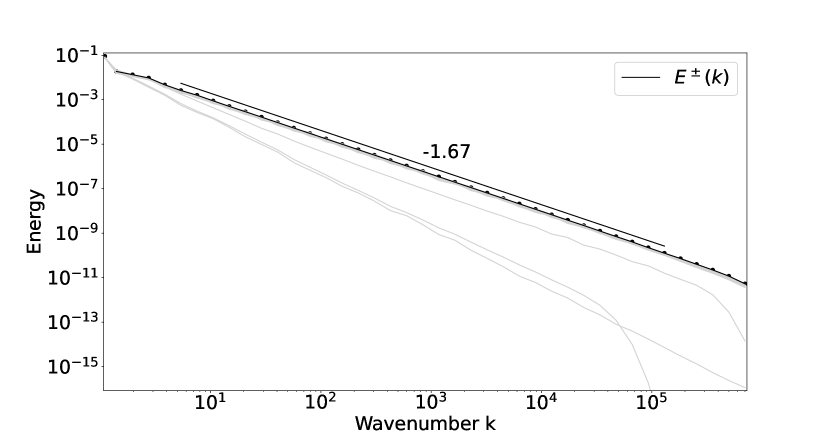
Figure 2: Averaged energy spectrum $E^{\pm}(k)$ (black) of the gradient diffusion network in spherical shell coordinates with single time-instances in gray showing the evolution from initial conditions towards a statistically steady state.

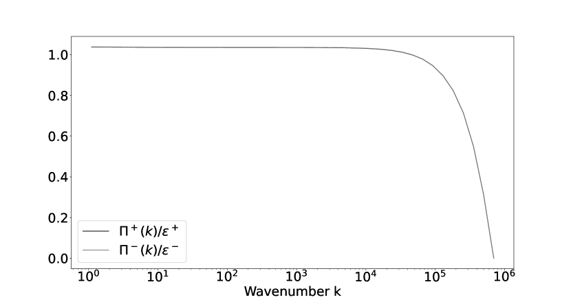
Figure 3: Averaged cross-scale energy flux $\Pi^{\pm}(k)$ of the gradient diffusion network in spherical shell coordinates normalized by the respective time-averaged dissipation rate $\varepsilon^{\pm}$.

V.2 Mean magnetic field influence

The inclusion of the anisotropic influence induced by a homogeneous mean magnetic on the nonlinear dynamics is carried out by the physically motivated modification of the transfer timescale (see Eq. (25)). This yields quasi-stationary power-law spectra with a different scaling behaviour compared to first numerical experiment described above. Initializing large-scale spectral energetic isotropy results in spectral scaling very close to an Iroshnikov-Kraichnan-like spectrum Kraichnan65 ; Irsoshnikov63 , $\leavevmode\nobreak\ k^{-3/2}$, shown in Fig. 5. The system exhibits constant averaged cross-scale flux, with an earlier dissipative fall-off as compared to the previous strong turbulence case, due to the weaker interaction and, consequently, a reduced nonlinear flux. Interestingly, Fig. 4 displays some spontaneous self-organization of the system with an emerging finite difference of the Elsaesser spectra, i.e. finite cross helicity due to alignment of $\mathbf{v}$ and $\mathbf{b}$. In the spectrally anisotropic large-scale setup, on the other hand, more complex dynamics evolve. To enhance the spectral resolution in the direction of the mean magnetic field, a cylindrical coordinate system is considered, with an increased number of field-parallel nodes in the direction of the external mean field is chosen. Theoretically and neglecting the difference between globally and locally orthogonal directions with respect to $\mathbf{b}$, a Kolmogorov spectrum is expected along the field-orthogonal direction and a weak turbulence spectrum, $\sim k_{\parallel}^{-2}$, along the field-parallel direction. Although the spectra display slight variations, see Fig. 7, the general behavior is captured and deviations can be explained by the model geometry. Due to the very sparse grid, the parallel and orthogonal interactions partially decouple in the low wave number region. However, the cylindrical shells that represent the spectral energy for a specific $k_{\bot}$ extend along the field-parallel direction over all wave numbers. As the parallel energy spectrum falls off at much lower parallel wave numbers than the orthogonal spectrum, this spectral anisotropy creates a non-homogenous set of active energy-containing nodes in the cylindrical shells determining the orthogonal energy spectrum. Consequently, the resulting spectral transfer function of our reduced model exhibits spectral variations, responsible for the irregularity in the orthogonal spectrum at the end of the approximate parallel scaling range. The pronounced anisotropy of the spectral energy flux is clearly shown in Fig. 8.

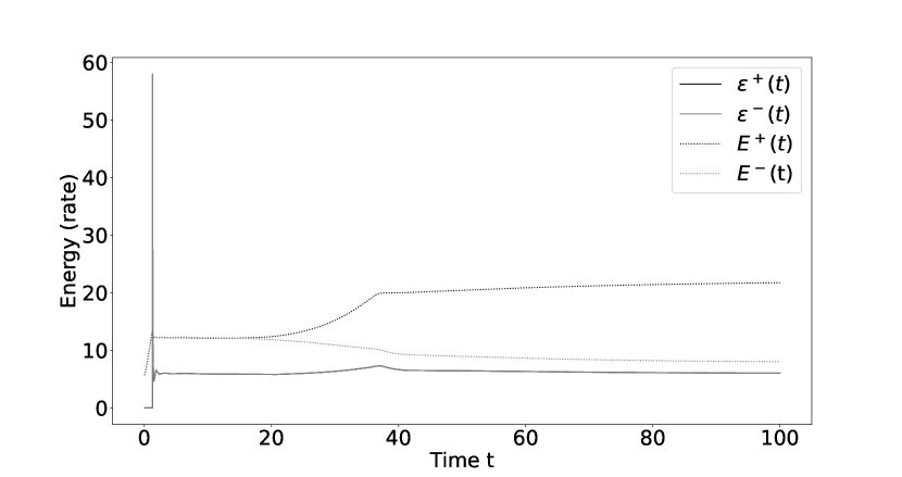
Figure 4: Elsässer energies $E^{\pm}$ (bottom) and dissipation rates $\varepsilon^{\pm}$ (top) with respect to their temporal evolution for spherical shell coordinates according to an energy flux timescale expressing mutual Alfvén-wave scattering (see Eq. (25)).

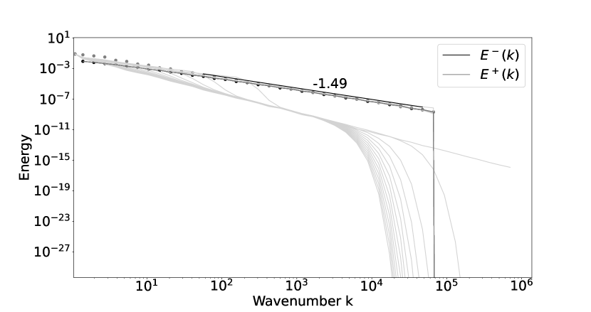
Figure 5: Averaged energy spectrum $E^{\pm}(k)$ (black) of the gradient diffusion network in spherical shell coordinates according to an energy flux timescale expressing mutual Alfvén-wave scattering (see Eq. (25)) with single instances in gray showing the evolution from initial conditions towards a statistically steady state.

Figure 6: Averaged cross-scale energy flux $\Pi^{\pm}(k)$ of the gradient diffusion network in spherical shell coordinates according to an the energy flux timescale expressing mutual Alfvén-wave scattering (see Eq. (25)) normalized by the average dissipation rate $\varepsilon^{\pm}$.

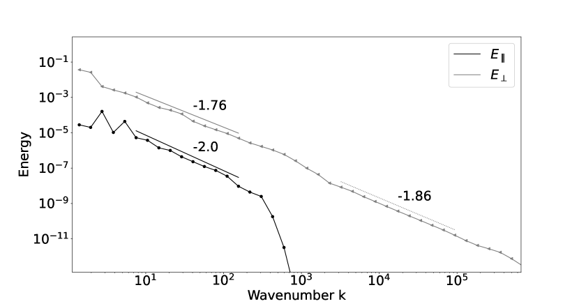
Figure 7: Averaged anisotropic energy spectrum $E_{\parallel,\perp}(k)$ of the gradient diffusion network in cylindrical shell coordinates according to a flux timescale incorporating the anisotropic influence of an externally imposed mean magnetic field.

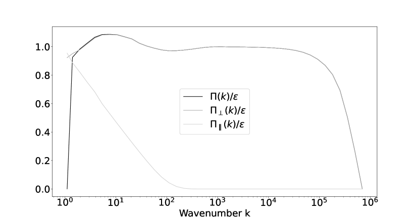
Figure 8: Averaged cross-scale energy fluxes $\Pi_{\parallel,\perp}(k)$ of the gradient diffusion network in cylindrical shell coordinates according to a flux timescale incorporating the anisotropic influence of an externally imposed mean magnetic field normalized by the average dissipation rate $\varepsilon$.

V.3 Decaying turbulence

An unforced gradient diffusion network establishes a Kolmogorov spectrum similar to the forced case while its total energy diminishes according to a power-law $E(t)\sim t^{-\beta}$ Kolmogorov1941 ; Saffman1967 ; biskamp:book ; BiskampMuller1999 . In contrast to hydrodynamic Navier-Stokes decay, the MHD case is reported to be significantly shallower due to the different structuring of the flow imposed by the additional magnetic field, i.e., $\beta\in[\frac{1}{2},1]$ biskamp:book ; BiskampMuller1999 ; Biskamp2000 (MHD) rather than $\beta\in[1,2]$Hinze ; Mohamed1990 ; Smith1993 (Navier-Stokes). Figure 9 reflects the behavior expected by hydrodynamic turbulence ($t^{-1.8}$), although the interaction of Elsässer variables is considered. Therefore, it is apparent that the model lacks dynamics likely related to magnetic helicity and its property to generate and preserve large-scale flow structures. The two Elsässer fields solely advect each other capturing nonlinear alignment effects and linear Alfvénic dynamics; the process of magnetic structure formation is not present in the current version of our reduced network model. This is an evident explanation of the different decay characteristics of the model as compared to direct numerical simulations (cf., e.g., BiskampMuller1999 ). Additionally, the universality of energy decay is in question as the decay exponent might be dependent on the configuration of the large-scale characteristics of the flow, which are hardly captured by the reduced model. The model, however, is not expected to be able to capture such complex dynamics yet, it rather offers a starting point to incorporate more sophisticated dynamics in its modular structure.

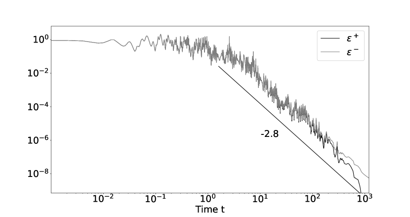
Figure 9: Decay of the dissipation rates $\varepsilon^{\pm}=\partial_{t}E^{\pm}(t)$ of the gradient diffusion network approximately indicating a $E^{\pm}(t)\sim t^{-1.8}$ power-law.

VI Conclusion

The present gradient-diffusion network model of magnetohydrodynamic turbulence combines phenomenological considerations and geometrical analysis of the nonlinear energy transfer function into a reduced-order representation of conservative spectral transport of energy and cross-helicity, which is formulated in port-Hamiltonian form.

Motivated by the fundamental Elsässer symmetry of the MHD equations, the dynamic network representation is based on an abstraction of the nonlinear triad interactions of MHD as a sum of conservative pair-exchanges of like-signed Elsässer energies. The third member of any interacting triad while not actively participating in the exchange of Elsässer energies takes the role of a mediator by setting the timescale of the transfer. An analysis of the mathematical structure of the exact Fourier transfer function allows to identify, next to the influence of the mediator, the important role played by the wave vector geometry of each triad for the amount of transferred energy. With these insights, the energy dynamics of incompressible turbulent flow can be modeled via a network made up of nodes corresponding to Fourier modes carrying two Elsässer energies. This reduced representation of turbulence has the general characteristics of a port-Hamiltonian model. Its modular structure allows straightforward and flexible changes to the size and shaping of the network which is a significant advantage compared to classical shell-models. Furthermore, the network ansatz has no limitations with regard to spatial dimensions. It is therefore not difficult to model anisotropic configurations that occur due to turbulent magnetic fields. The principal control parameters of the model are the dominant timescales of nonlinear interaction. Due to the sparse discretization of Fourier space that is possible in the network architecture, the model can attain a spectral bandwidth and associated Reynold numbers which are comparable to classic shell-models, however, without sharing their structural restrictions.

Numerical experiments testing the basic properties such as consistency, and stability, of the model system show stationary self-similar inertial-range solutions of MHD energy spectra and spectral fluxes in agreement with theoretical expectations and results from direct numerical simulations. By simple extension of the set of underlying timescales, the model also allows to correctly reproduce anisotropic behaviour expected in systems permeated by a constant mean magnetic field. Simple tests with regard to turbulence decay also gave results consistent with present knowledge.

Although these encouraging results demonstrate the basic functionality and consistency of the model, some fundamental dynamic properties of incompressible turbulent MHD still need to be included in the reduced representation. An important next step towards a more comprehensive physical representation is the inclusion of the third ideal invariant of incompressible MHD, magnetic helicity, $H^{M}=1/(2V)\int\mathrm{d}V\mathbf{a}\cdot\mathbf{b}$, with the magnetic vector potential $\mathbf{a}$, $\mathbf{b}=\nabla\times\mathbf{a}$. This quantity is responsible for the formation of large-scale magnetic structures from small-scale MHD turbulence. As such large-scale structures have a profound effect on turbulent dynamics and energetic modelling of magnetic helicity will be the next step of development and is currently under way.

- [1] D. E. Ashpis, T. B. Gatski, and R. Hirsh, editors. Instabilities and Turbulence in Engineering Flows. Kluwer, Dordrecht, 1993.
- [2] V. Berionni and Ö.D. Gürcan. Predator prey oscillations in a simple cascade model of drift wave turbulence. Physics of Plasmas, 18, 2011.
- [3] L. Biferale. Shell models of energy cascade in turbulence. Annual Review of Fluid Mechanics, 35:441–468, 2003.
- [4] D. Biskamp. Nonlinear Magnetohydrodynamics. Cambridge University Press, Cambridge, 1993.
- [5] D. Biskamp. Magnetohydrodynamic Turbulence. Cambridge University Press, Cambridge, 2003.
- [6] D. Biskamp and W.-C. Müller. Decay laws for three-dimensional magnetohydrodynamic turbulence. Physical Review Letters, 83, 1999.
- [7] D. Biskamp and W.-C. Müller. Scaling properties of three-dimensional isotropic magnetohydrodynamic turbulence. Physics of Plasmas, 7(12), 2000.
- [8] R. Bruno and V. Carbone. The solar wind as a turbulence laboratory. Living Review in Solar Physics, 2(4), 2005. http://www.livingreviews.org/lrsp-2005-4.
- [9] P. Constantin and A. Majda. The beltrami spectrum for incompressible flows. Common. Math. Phys., (115):435–456, 1988.
- [10] P. D. Ditlevsen. Turbulence and Shell Models. Cambridge University Press, 2011.
- [11] B. G. Elmegreen and J. Scalo. Interstellar turbulence I: Observations and processes. Annual Review of Astronomy and Astrophysics, 42:211–273, 2004.
- [12] W. M. Elsasser. The hydromagnetic equations. Physical Review, 79:183, 1950.
- [13] G. Eyink, E. Vishniac, C. Lalescu, H. Aluie, K. Kanov, K. Bürger, R. Burns, C. Meneveau, and A. Szalay. Flux-freezing breakdown in high-conductivity magnetohydrodynamic turbulence. Nature Letter, 497:466–469, 2013.
- [14] C. Federrath, R. S. Klessen, L. Iapichino, and J. R. Beattie. The sonic scale of interstellar turbulence. Nature Astronomy, 5:365–371, 2021.
- [15] U. Frisch. Turbulence. Cambridge University Press, Cambridge, 1996.
- [16] J. O. Hinze. Turbulence. McGraw-Hill, New York, 1987.
- [17] P.S. Iroshnikov. Turbulence of a conducting fluid in a strong magnetic field. Astronomicheskii Zhurnal, 40:742, 1963.
- [18] T. Ishihara, T. Gotoh, and Y. Kaneda. Study of high-reynolds-number isotropic turbulence by direct numerical simulation. Annual Review of Fluid Mechanics, 41:165–180, 2009.
- [19] A. N. Kolmogorov. On the degeneration of isotropic turbulence in an incompressible viscous liquid. Doklady Akademiia Nauk SSSR, 31, 1941.
- [20] R. H. Kraichnan. Inertial-range transfer in two- and three-dimensional turbulence. J. Fluid Mech., 47:525–535, 1971.
- [21] R.H. Kraichnan. Inertial-range spectrum of hydromagnetic turbulence. The physics of fluids, 8, 1965.
- [22] T. D. Lee. On some statistical properties of hydrodynamical and magneto-hydrodynamical fields. Quarterly of Applied Mathematics, 10(1):69–74, 1952.
- [23] M. Linkmann, A. Berera, M. McKay, and J. Jäger. Helical mode interactions and spectral transfer process in magnetohydrodynaic turbulence. J. Fluid Mech., 791:61–96, 2016.
- [24] V. Mehrmann and R. Morandin. Structure-preserving discretization for port-hamiltonian descriptor systems. arXiv:1903.10451, 2019.
- [25] H. K. Moffatt. The degree of knottedness of tangled vortex lines. Journal of Fluid Mechanics, 35(1):117–129, 1969.
- [26] H.K. Moffatt. Note on the triad interactions of homogeneous turbulence. J. Fluid Mech., 741, 2014.
- [27] M. S. Mohamed and J. C. LaRue. The decay power law in grid-generated turbulence. Journal of Fluid Mechanics, 219, 1990.
- [28] A further reduction to three real and complex components to reduce the system’s complexity is possible, but not employed in this work.
- [29] F. Peters and C. Marrasé. Effects of turbulence on plankton: an overview of experimental evidence and some theoretical considerations. Marine Ecology Progress Series, 205:291–306, 2000.
- [30] F. Plunian, R. Stepanov, and P. Frick. Shell models of magneto turbulence. Physics Reports, 2013.
- [31] S. B. Pope. Turbulent Flows. Cambridge University Press, Cambridge, 2000.
- [32] N.M. Rathmann and P.D. Ditlevsen. Pseudo-invariants contributing to inverse energy cascades in three-dimensional turbulence. Physical Review Fluids, (2), 2017.
- [33] H. A. Rose and P. L. Sulem. Fully developed turbulence and statistical mechanics. Journal de Physique, 39(5):441–483, 1978.
- [34] P. G. Saffman. Note on decay of homogeneous turbulence. Physics of Fluids, 10, 1967.
- [35] J. P. L. C. Salazar and L. R. Collins. Two-particle dispersion in isotropic turbulent flows. Annual Review of Fluid Mechanics, 41:405–432, 2009.
- [36] R. M. Samelson. Lagrangian motion, coherent structures, and lines of persistent material strain. Annual Review of Marine Science, 5:137–163, 2013.
- [37] M. R. Smith, R. J. Donnelly, N. Goldenfeld, and Vinen W. F. Decay of vorticity in homogeneous turbulence. Physical Review Letters, 71, 1993.
- [38] A. van der Schaft and D. Jeltsema. Port-hamiltonian systems theory: An introductory overview. foundations and trends. Systems and Control, 1(2-3):173–378, 2014.
- [39] F. Waleffe. Inertial transfers in the helical decomposition. Physics of Fluids A: Fluid Dynamics, (5), 1992.
- [40] F. Waleffe. The nature of triad interactions in homogeneous turbulence. Physics of Fluids A: Fluid Dynamics, 4, 1992.