NOSNOC: A Software Package for Numerical Optimal Control of Nonsmooth Systems

Abstract

This letter introduces the NOnSmooth Numerical Optimal Control (NOSNOC) open-source software package. It is a modular MATLAB tool based on CasADi and IPOPT for numerically solving Optimal Control Problems (OCP) with piecewise smooth systems (PSS). The tool supports: 1) automatic reformulation of systems with state jumps into PSS (via the time-freezing reformulation [1]) and of PSS into computationally more convenient forms, 2) automatic discretization of the OCP via, e.g., the recently introduced Finite Elements with Switch Detection [2] which enables high accuracy optimal control and simulation of PSS, 3) solution methods for the resulting discrete-time OCP. The nonsmooth discrete-time OCP are solved with techniques of continuous optimization in a homotopy procedure, without the use of integer variables. This enables the treatment of a broad class of nonsmooth systems in a unified way. Two tutorial examples are given. A benchmark shows that NOSNOC provides both faster and more accurate solutions than conventional approaches, including mixed-integer formulations.

software, hybrid systems, optimal control, numerical algorithms

1 Introduction

Nonsmooth and hybrid dynamical systems are a powerful tool to model complex physical and cyber-physical phenomena. Their theory is well established and many good numerical simulation algorithms exist [3]. However, optimal control of nonsmooth systems is yet not wide spread, mainly due to the computational difficulty and lack of software. A notable exception are mixed integer optimization approaches [4]. However, they become intractable as soon as nonconvexities appear or exact junction times need to be computed. The open-source software package NOSNOC is designed to reduce this gap [5]. We regard a nonsmooth OCP of the following form:

$$\min_{x(\cdot),u(\cdot)}\quad \int_{0}^{T}f_{\mathrm{q}}(x(t),u(t)){\mathrm{d}}t+f_{\mathrm{T}}(x(T))$$ (1a)

$$\textrm{s.t.}\quad x_{0} =s_{0},$$ (1b)

$$\dot{x}(t) \!=\!f_{i}(x(t),u(t)),\ \!\mathrm{if}\ \!x\!\in\!R_{i},\ \!i\!\in\!\mathcal{I},t\in[0,\!T],$$ (1c)

$$0 \geq G_{\mathrm{ineq}}(x(t),u(t)),\ t\in[0,T],$$ (1d)

$$0 \geq G_{\mathrm{T}}(x(T)),$$ (1e)

where $f_{\mathrm{q}}:{\mathbb{R}}^{n_{x}}\times{\mathbb{R}}^{n_{u}}\to{\mathbb{R}}$ is the stage cost and $f_{\mathrm{T}}:{\mathbb{R}}^{n_{x}}\to{\mathbb{R}}$ is the terminal cost, $s_{0}\in{\mathbb{R}}^{n_{x}}$ is a given parameter. The path and terminal constraints are collected in the functions $G_{\mathrm{ineq}}:{\mathbb{R}}^{n_{x}}\times{\mathbb{R}}^{n_{u}}\to{\mathbb{R}}^{n_{g1}}$ and $G_{\mathrm{T}}:{\mathbb{R}}^{n_{x}}\to{\mathbb{R}}^{n_{g2}}$, respectively. The ODE (1c) is a piecewise smooth system (PSS), where $\mathcal{I}\coloneqq\{1,\ldots,{n_{f}}\}$. The regions $R_{i}$ are disjoint, nonempty, connected and open. The functions $f_{i}(\cdot)$ are smooth on an open neighborhood of $\overline{R_{i}}$, which denotes the closure of ${R}_{i}$.

The event of $x$ reaching some boundary $\partial R_{i}$ is called a switch. The right-hand side (r.h.s.) of (1c) is in general discontinuous in $x$. Several classes of systems with state jumps can be brought into the form of (1c) via the time-freezing reformulation [1, 6, 7]. Thus, the focus on PSS enables a unified treatment of many different kinds of nonsmooth systems.

One might wonder why not just to apply standard direct methods and existing software to problem with a smoothed version of the r.h.s. of (1c)? The necessity for tailored methods and software follows from two important results from the seminal paper of Stewart and Anitescu [8]. First, in standard direct approaches for (1c), the numerical sensitivities are wrong no matter how small the integrator step-size is. This often yields artificial local minima and impairs the optimization progress [9]. Second, smoothing delivers correct sensitivities only if the step-size shrinks faster than the smoothing parameter. Consequently, even for moderate accuracy, many optimization variables are needed.

These two difficulties are overcome by the recently introduced Finite Elements with Switch Detection (FESD) method [2]. In this method, the ODE (1c) is transformed into a Dynamic Complementarity System (DCS). FESD relies on Runge-Kutta (RK) discretizations of the DCS, but the integrator step-sizes are left as degrees of freedom as first proposed by [10]. Additional constraints ensure implicit and exact switch detection and eliminate spurious degrees of freedom. The discretization yields Mathematical Programs with Complementarity Constraints (MPCC). They are highly degenerate and nonsmooth Nonlinear Programs (NLP) [11, 12], but with suitable reformulations and homotopy procedures they can be solved efficiently using techniques for smooth NLP, without any integer variables.

The MATLAB tool NOSNOC [5] aims to automate the whole tool-chain and to make nonsmooth optimal control problems solvable for non-experts. In particular, it supports:

• automatic model reformulation of the PSS (1c) into the computationally more suitable DCS.

• time-freezing reformulation for systems with state jumps, reformulations to solve time-optimal control problems both for PSS and systems with state jumps,

• automatic discretization of the OCP (1) via FESD or RK,

• several algorithms for solving the MPCC with a homotopy approach,

• rapid prototyping with different formulations and algorithms for nonsmooth OCP.

It builds on the open-source software packages: CasADi [13] which is a symbolic framework for nonlinear optimization and the NLP solver IPOPT[14]. Having these packages as a back-end enables good computational performance, despite the fact that all user inputs are provided in MATLAB. All steps above can be performed in a couple of lines of code without needing a deep understanding of the numerical methods and implementation details. In NOSNOC, the user has only to specify the functions in (1) and the sets $R_{i}$ via constraint functions $c(x)$, cf. Section 2. The reformulation, discretization and solution of the nonsmooth OCP is completely automated.

Notation

The complementarity conditions for two vectors $a,b\in{\mathbb{R}}^{n}$ read as ${0\leq a\perp b\geq 0}$, where $a\perp b$ means $a^{\top}b=0$. The so-called C-functions $\Phi:{\mathbb{R}}^{n}\times{\mathbb{R}}^{n}\to{\mathbb{R}}^{n}$ have the property $\Phi(a,b)=0\!\!\iff\!\!{0\leq a\perp b\geq 0}$, e.g., $\Phi(a,b)=\min(a,b)$. The concatenation of two column vectors $a\in{\mathbb{R}}^{n_{a}}$, $b\in{\mathbb{R}}^{n_{b}}$ is denoted by $(a,b)\coloneqq[a^{\top},b^{\top}]^{\top}$, the concatenation of several column vectors is defined in an analogous way. A column vector with all ones is denoted by $e=(1,1,\dots,1)\in{\mathbb{R}}^{n}$, its dimensions is clear from the context. The closure of a set $C$ is denoted by $\overline{C}$, its boundary as $\partial C$. Given a matrix $M\in{\mathbb{R}}^{n\times m}$, its $i$-th row is denoted by $M_{i,\bullet}$ and its $j$-th column is denoted by $M_{\bullet,j}$.

Outline

Section 2 describes the reformulation of PSS into DCS. Section 3 describes the discretization methods in NOSNOC  with a focus on FESD. In Section 4, solution strategies for the discrete-time OCP are discussed. Section 5 provides two tutorials for the use of NOSNOC and a numerical benchmark. Section 6 outlines some future developments.

2 Problem Reformulation

System with state jumps do not fit in the form of (1c). However, we use the time-freezing reformulation [1, 7, 6] to automatically reformulate them into the from of (1c). An example is given in Section 5.3.

In this section, we detail how to compactly represent the systems (1c) and a how to transform them into a Dynamic Complementarity System (DCS) via Stewart’s approach [15].

It is assumed that $\overline{\bigcup\limits_{i\in\mathcal{I}}R_{i}}={\mathbb{R}}^{n}$ and that ${\mathbb{R}}^{n}\setminus\bigcup\limits_{i\in\mathcal{I}}R_{i}$ is a set of measure zero. Moreover, we assume that $R_{i}$ are defined via the zero level sets of the components of the smooth function $c:{\mathbb{R}}^{n_{x}}\to{\mathbb{R}}^{n_{c}}$. We use a sign matrix $S\in{\mathbb{R}}^{{n_{f}}\times n_{c}}$ with non repeating rows for a compact representations as follows:

$$S =\begin{bmatrix}1&1&\dots&1&1\\ \vspace{-0.05cm}1&1&\dots&1&-1\\ \vspace{-0.08cm}\vdots&\vdots&\dots&\vdots\\ \vspace{-0.08cm}-1&-1&\dots&-1&-1\\ \end{bmatrix},$$ (2a)

$$R_{i} =\{x\in{\mathbb{R}}^{n_{x}}\mid\mathrm{diag}(S_{i,\bullet})c(x)>0\}.$$ (2b)

For example, for the sets $R_{1}=\{x\in{\mathbb{R}}\mid x>0\}$ and $R_{2}=\{x\in{\mathbb{R}}\mid x<0\}$, we have $c(x)=x$ and $S=\begin{bmatrix}1&-1\end{bmatrix}^{\top}$.

The dynamics are not defined on $\partial R_{i}$ and to have a meaningful notion of solution for the PSS (1c) we use the Filippov convexification and define the following differential inclusion [16]:

$$\begin{split}\dot{x}\in F_{\mathrm{F}}(x,u)=&\Big{\{}F(x)\theta\mid\sum_{i\in{\mathcal{I}}}\theta_{i}=1,\ \theta_{i}\geq 0,\ \theta_{i}=0\ \\ &\mathrm{if}\;x\notin\overline{R_{i}},\forall i\in{\mathcal{I}}\Big{\}},\end{split}$$ (3)

where $\theta=(\theta_{1},\ldots,\theta_{{n_{f}}})\in{\mathbb{R}}^{{n_{f}}}$ and $F(x)\coloneqq[f_{1}(x),\ldots,f_{{n_{f}}}(x)]\in{\mathbb{R}}^{n_{x}\times{n_{f}}}$. Note that in the interior of a set $R_{i}$ we have $F_{\mathrm{F}}(x)=\{f_{i}(x)\}$ and on the boundary between some regions the resulting vector field is a convex combination of the neighboring vector fields. To have a computationally useful representation of the Filippov system (3), we transform it into a DCS via Stewart’s reformulation [15]. In this reformulation, it is assumed that the sets $R_{i}$ are represented via the discriminant functions $g_{i}(\cdot)$:

$$R_{i}=\{x\in{\mathbb{R}}^{n_{x}}\mid g_{i}(x)<\min_{j\in{\mathcal{I}}\!,\,j\neq i}g_{j}(x)\}.$$ (4)

Given the more intuitive representation via the sign matrix $S$ in Eq. (2), it can be shown that the function $g:{\mathbb{R}}^{n_{x}}\to{\mathbb{R}}^{{n_{f}}}$ whose components are $g_{i}(x)$ can be found as [2]:

$$g(x)=-Sc(x).$$ (5)

With this representation, the convex multipliers in the r.h.s. of (3) can be found as a solution of a suitable Linear Program (LP) [15], and (3) is equivalent to

$$\dot{x}=F(x,u)\theta(x),$$ (6a)

$$\theta(x)\in\arg\min_{\tilde{\theta}\in{\mathbb{R}}^{{n_{f}}}}\quad g(x)^{\top}\,\tilde{\theta}\quad\textrm{s.t.}\quad e^{\top}\tilde{\theta}=1,\ \tilde{\theta}\geq 0.$$ (6b)

We use a C-function $\Phi(\cdot,\cdot)$ for the complementarity conditions and write the KKT conditions of the LP (6b) as a nonsmooth equation

$$G_{{\mathrm{LP}}}(x,\theta,\lambda,\mu) \coloneqq\begin{bmatrix}g(x)-\lambda-\mu e\\ 1-e^{\top}\theta\\ \Phi(\theta,\lambda)\end{bmatrix}=0,$$ (7)

where $\lambda\in{\mathbb{R}}^{n_{f}}_{\geq 0}$ and $\mu\in{\mathbb{R}}$ are the Lagrange multipliers associated with the constraints of the LP (6b). Note that $\mu=\min_{j\in{\mathcal{I}}}g_{j}(x)$. Finally, the Filippov system is equivalent to the following DCS, which can be interpreted as a nonsmooth differential algebraic equation:

$$\dot{x} =F(x,u)\theta,\quad 0=G_{{\mathrm{LP}}}(x,\theta,\lambda,\mu).$$ (8)

A fundamental property of the multipliers $\lambda(\cdot)$ and $\mu(\cdot)$ is their continuity in time [2, Lemma 5], whereas $\theta(\cdot)$ is in general a discontinuous function in time.

3 The Standard and FESD Discretizations for a Single Control Interval

This section describes the discretization of a single control interval in NOSNOC via standard RK methods and FESD. We start with a standard RK method for the DCS (8). We subsequently introduce step-by-step the additional constraints which lead to FESD.

3.1 Standard Runge-Kutta Discretization

We consider a single control interval $[0,T]$ with a given constant control input $q$ and a given initial value $x_{0}=s_{0}$. We divide the control interval into ${N_{\mathrm{FE}}}$ finite elements (i.e., integration intervals) $[t_{n},t_{n+1}]$ via the grid points $0=t_{0}<t_{1}<\ldots<t_{{N_{\mathrm{FE}}}}=T$. On each of these intervals, we apply an ${n_{\mathrm{s}}}$-stage RK scheme, which is defined by its Butcher tableau entries $a_{i,j},\;b_{i},\;c_{i},\;i,j\in\{1,\ldots,{n_{\mathrm{s}}}\}$ [17]. We denote the step-size as $h_{n}=t_{n+1}-t_{n},\;n=0,\ldots,{N_{\mathrm{FE}}}-1$. The approximation of the state at the grid points $t_{n}$ is denoted by $x_{n}\approx x(t_{n})$. The time derivative of the state at the stage points $t_{n}+c_{i}h_{n},\;i=1,\ldots,{n_{\mathrm{s}}}$, for a single finite element are collected in the vector $V_{n}\coloneqq(v_{n,1},\ldots,v_{n,{n_{\mathrm{s}}}})\in{\mathbb{R}}^{{n_{\mathrm{s}}}\cdot n_{x}}$. The stage values for the algebraic variable $\theta(\cdot)$ are collected in $\Theta_{n}\coloneqq(\theta_{n,1},\ldots,\theta_{n,{n_{\mathrm{s}}}})\in{\mathbb{R}}^{{n_{\mathrm{s}}}\cdot{n_{f}}}$. The vectors $\Lambda_{n}\in{\mathbb{R}}^{{n_{\mathrm{s}}}\cdot{n_{f}}}$ and $M_{n}\in{\mathbb{R}}^{{n_{\mathrm{s}}}}$ are defined accordingly. Let $x_{n}^{\mathrm{next}}$ denote the value at the next time step $t_{n+1}$, which is obtained after a single RK step.

Now we can write the RK equations for the DCS (8) in a compact differential form. We summarize all RK equations of a finite element in $G_{{\mathrm{rk}}}(x_{n}^{\mathrm{next}},Z_{n},h_{n},q)=0$, where $Z_{n}=(x_{n},\Theta_{n},\Lambda_{n},M_{n},V_{n})$ collects all internal variables, and define

$$\begin{split}&G_{{\mathrm{rk}}}(x_{n}^{\mathrm{next}},Z_{n},h_{n},q)\!\coloneqq\!\!\!\\ &\begin{bmatrix}\!v_{n,1}\!-\!F(x_{n}+h_{n}\sum_{j=1}^{{n_{\mathrm{s}}}}a_{1,j}v_{n,j},q)\theta_{n,1}\\ \vdots\\ v_{n,{n_{\mathrm{s}}}}\!-\!F(x_{n}+h_{n}\sum_{j=1}^{{n_{\mathrm{s}}}}a_{{n_{\mathrm{s}}},j}v_{n,j},q)\theta_{n,{n_{\mathrm{s}}}}\\ G_{{\mathrm{LP}}}(x_{n}+h_{n}\sum_{j=1}^{{n_{\mathrm{s}}}}a_{1,j}v_{n,j},\theta_{n,1},\lambda_{n,1},\mu_{n,1})\\ \vdots\\ G_{{\mathrm{LP}}}(x_{n}+h_{n}\sum_{j=1}^{{n_{\mathrm{s}}}}a_{{n_{\mathrm{s}}},j}v_{n,j},\theta_{n,{n_{\mathrm{s}}}},\lambda_{n,{n_{\mathrm{s}}}},\mu_{n,{n_{\mathrm{s}}}})\\ x_{n}^{\mathrm{next}}-x_{n}-h_{n}\sum_{i=1}^{{n_{\mathrm{s}}}}b_{i}v_{n,i}\end{bmatrix}.\end{split}$$

To summarize all conditions for a single control interval in a compact way, we introduce some new notation. The variables for all finite elements of a single control interval are collected in the following vectors $\mathbf{x}=(x_{0},x_{0}^{\mathrm{next}},\ldots,x_{{N_{\mathrm{FE}}}})\in{\mathbb{R}}^{(2{N_{\mathrm{FE}}}+1)n_{x}}$, $\mathbf{V}=(V_{0},\ldots,V_{{N_{\mathrm{FE}}}-1})\in{\mathbb{R}}^{{N_{\mathrm{FE}}}{n_{\mathrm{s}}}n_{x}}$ and $\mathbf{h}\coloneqq(h_{0},\ldots,h_{{N_{\mathrm{FE}}}-1})\in{\mathbb{R}}^{{N_{\mathrm{FE}}}}$. The vectors $\mathbf{\Theta}\in{\mathbb{R}}^{{N_{\mathrm{FE}}}{n_{\mathrm{s}}}{n_{f}}}$, $\mathbf{\Lambda}\in{\mathbb{R}}^{{N_{\mathrm{FE}}}{n_{\mathrm{s}}}{n_{f}}}$ and $\mathbf{M}\in{\mathbb{R}}^{{N_{\mathrm{FE}}}{n_{\mathrm{s}}}}$ are defined analogously. The vector $\mathbf{Z}=(\textbf{x},\mathbf{\Theta},\mathbf{\Lambda},\mathbf{M},\mathbf{V})$ collects all internal variables.

Finally, we can summarize all computations over a single control interval and interpret it as a discrete-time nonsmooth system:

$${s}_{1}\!=\!F_{\mathrm{std}}(\mathbf{Z}),\,0\!=\!G_{\mathrm{std}}(\mathbf{Z},\mathbf{h},s_{0},q)$$ (9)

with $F_{\mathrm{std}}(\mathbf{Z})=x_{{N_{\mathrm{FE}}}}$ and

$$G_{\mathrm{std}}(\mathbf{Z},\mathbf{h},s_{0},q)\coloneqq \begin{bmatrix}x_{0}-s_{0}\\ G_{{\mathrm{rk}}}(x_{0}^{\mathrm{next}},Z_{0},h_{0},q)\\ x_{1}-x_{0}^{\mathrm{next}}\\ \vdots\\ G_{{\mathrm{rk}}}(x_{{N_{\mathrm{FE}}}-1}^{\mathrm{next}},Z_{{N_{\mathrm{FE}}}-1},h_{{N_{\mathrm{FE}}}-1},q)\\ x_{{N_{\mathrm{FE}}}}-x_{{N_{\mathrm{FE}}}-1}^{\mathrm{next}}\end{bmatrix}.$$

Note that we keep a dependency on ${h}_{n}$ in (9), but ${h}_{n}$ is implicitly given by the chosen discretization grid. This also means that for a standard RK scheme for DCS, higher order accuracy can be achieved only if the grid points $t_{n}$ coincide with all switching points, which is in practice impossible to achieve.

3.2 Cross-Complementarity

In FESD, the step-sizes $h_{n}$ are left as degrees of freedom such that the grid points $t_{n}$ can coincide with the switching times. Consequently, the switches should not happen on the stages inside a finite element. To exploit the additional degrees of freedom and to achieve these two effects we introduce additional conditions to the RK equations (9) called cross complementaries. A key assumption, of course, is that there are more grid points in the interior of the grid than switching points.

For ease of exposition, we focus on the case where the right-boundary point of a finite element is also an RK-stage point, i.e., $c_{{n_{\mathrm{s}}}}=1$ and $t_{n+1}=t_{n}+c_{{n_{\mathrm{s}}}}h_{n}$. Extensions can be found in [2]. To achieve implicit and exact switch detection at the boundaries of $[t_{n},t_{n+1}]$ and to avoid switching inside an element we exploit the fact that $\lambda(\cdot)$ and $\mu(\cdot)$ are continuous functions. We need their values at $t_{n}$ and $t_{n+1}$ which are denoted by $\lambda_{n,0},\;\mu_{n,0}$ and $\lambda_{n,{n_{\mathrm{s}}}},\;\mu_{n,{n_{\mathrm{s}}}}$, respectively. Due to continuity, we impose that $\lambda_{n,{n_{\mathrm{s}}}}=\lambda_{n+1,0}$ and $\mu_{n,{n_{\mathrm{s}}}}=\mu_{n+1,0}$ and use only the right boundary points of the finite elements ($\lambda_{n,{n_{\mathrm{s}}}}$ and $\mu_{n,{n_{\mathrm{s}}}}$) in the sequel. To achieve the effects described above, we introduce the cross complementarity conditions which read as [2]:

$$0\!=\!G_{\mathrm{cross}}(\mathbf{\Theta},\mathbf{\Lambda})\!\!\coloneqq\!\!\begin{bmatrix}\sum_{i=1}^{{n_{\mathrm{s}}}}\!\sum_{j=1,j\neq i}^{{n_{\mathrm{s}}}}\theta_{1,i}^{\top}\lambda_{1,j}\\ \vdots\\ \sum_{i=1}^{{n_{\mathrm{s}}}}\!\sum_{\begin{subarray}{c}j=0,\\ j\neq i\end{subarray}}^{{n_{\mathrm{s}}}}\theta_{{N_{\mathrm{FE}}}\!-\!1,i}^{\top}\lambda_{{N_{\mathrm{FE}}}\!-\!1,j}\end{bmatrix}.$$ (10)

This additional constraint ensures two very important properties: (i) we have the same active-set in (9) in $\Phi(\theta_{n,m},\lambda_{n,m})$ for all $m$ and changes can happen only for different $n$, i.e., at grid points $t_{n}$, (ii) whenever the active-sets for two neighboring finite elements differ in the $i$-th and $j$-th components of $\Phi(\theta_{n,m},\lambda_{n,m})$, then these two components of $\lambda_{n,{n_{\mathrm{s}}}}$ must be zero [2]. This will implicitly result in the constraint $0=g_{i}(x_{n+1})-g_{j}(x_{n+1})$ (which comes from (7) and the fact that $\mu_{n,{n_{\mathrm{s}}}}=\min_{j}g_{j}(x_{n+1})$). This defines the boundary between regions and $R_{i}$ and $R_{j}$, cf. (4). Thus, it implicitly forces $h_{n}$ to adapt for exact switch detection.

3.3 Step-Equilibration

If no switches occur then also no active-set changes happen, hence the constraints (10) are trivially satisfied. Consequently, the step-size $h_{n}$ can vary in a possibly undesired way and the optimizer can play with the discretization accuracy. To remove the spurious degrees of freedom we introduce an indicator function $\eta(\cdot)$ evaluated at the inner grid points $t_{n},\;n=1,\dots,{N_{\mathrm{FE}}}-1$ and its value at $t_{n}$ is denoted by $\eta_{n}$. It has the following property: if a switch happens at $t_{n}$ its value is zero, otherwise it is strictly positive. We omit the details on how a function $\eta(\cdot)$ is derived and refer to [2]. The discrete-time function $\eta(\cdot)$ depends on the values of $\Theta_{n}$ and $\Lambda_{n}$ of neighboring finite elements and we define

$$\eta_{n}(\mathbf{\Theta},\mathbf{\Lambda})\coloneqq\eta(\Theta_{n-1},\Lambda_{n-1},\Theta_{n},\Lambda_{n}).$$

Thus, the constraint $0=G_{\mathrm{eq}}(\mathbf{h},\mathbf{\Theta},\mathbf{\Lambda})$ removes the possible spurious degrees of freedom in $h_{n}$, where:

$$G_{\mathrm{eq}}(\mathbf{h},\mathbf{\Theta},\mathbf{\Lambda})\!\!\coloneqq\!\!\!\begin{bmatrix}(h_{1}-h_{0})\eta_{1}(\mathbf{\Theta},\!\mathbf{\Lambda})\\ \vdots\\ (h_{{N_{\mathrm{FE}}}\!-\!1}-h_{{N_{\mathrm{FE}}}\!-\!2})\eta_{{N_{\mathrm{FE}}}\!-\!1}(\mathbf{\Theta},\!\mathbf{\Lambda})\\ \end{bmatrix}\!\!.$$ (11)

We call the condition (11) step-equilibration. A consequence of (11) are locally equidistant state discretization grids between switching point, within a single control interval. Since this constraint can be quite nonlinear, NOSNOC offers several reformulations and heuristics that help numerical convergence.

3.4 Finite Elements with Switch Detection

We now use the ingredients explained above to state the FESD method. Similar to the standard RK scheme (9), we summarize all computations over a single control interval and interpret it as a discrete-time nonsmooth system where internally exact switch detection is happening. The next step is computed by

$$s_{1}\!=\!F_{{\mathrm{fesd}}}(\mathbf{Z}),\ \!0\!=\!G_{{\mathrm{fesd}}}(\mathbf{Z},\mathbf{h},s_{0},q,T),$$ (12)

and $F_{{\mathrm{fesd}}}(\mathbf{Z})\!=x_{{N_{\mathrm{FE}}}}$ renders the state transition map and the equation $0=G_{{\mathrm{fesd}}}(\mathbf{x},\mathbf{Z},q)$ collects all other internal computations including all RK steps within the regarded control interval:

$$G_{{\mathrm{fesd}}}(\mathbf{Z},\mathbf{h},s_{0},q,T)\!\coloneqq\!\!\begin{bmatrix}G_{\mathrm{std}}(\mathbf{Z},\mathbf{h},s_{0},q)\\ G_{\mathrm{cross}}(\mathbf{\Theta},\mathbf{\Lambda})\\ G_{\mathrm{eq}}(\mathbf{h},\mathbf{\Theta},\mathbf{\Lambda})\\ \sum_{n=0}^{{N_{\mathrm{FE}}}-1}h_{n}-T\end{bmatrix}.$$

The last condition ensures that the length of the considered time-interval is unaltered. In contrast to (9), $h_{n}$ are now degrees of freedom, $s_{0},q$ and $T$ are given parameters. The formulation (12) can be used as an integrator with exact switch detection for PSS (1c). This feature is implemented in NOSNOC via the function integrator_fesd(). It can automatically handle all kinds of switching cases such as: crossing a discontinuity, sliding mode, leaving a sliding mode or spontaneous switches [16].

4 Discretizing and Solving a Nonsmooth Optimal Control Problem

This section outlines how a nonsmooth OCP is discretized in NOSNOC and how the resulting MPCC is solved.

4.1 Multiple Shooting-Type Discretization with FESD

One of the main goals of NOSNOC is to numerically solve a discretized version of the OCP (1). We consider ${N}_{\mathrm{stg}}\geq 1$ control intervals of equal length, indexed by $k$, with piecewise constant controls collected in $\mathbf{q}=(q_{0},\ldots,q_{{N}_{\mathrm{stg}}-1})\in{\mathbb{R}}^{{N}_{\mathrm{stg}}n_{u}}$. All internal variables are additionally equipped with an index $k$. On every control interval $k$, we apply an FESD discretization (12) with $N_{\mathrm{FE}}$ internal finite elements. The state values at the control interval boundaries are collected in $\mathbf{s}=(s_{0},\ldots,s_{{N}_{\mathrm{stg}}})\in{\mathbb{R}}^{({N}_{\mathrm{stg}}+1)n_{x}}$. The vector ${\mathcal{Z}}=(\mathbf{{Z}}_{0},\ldots,\mathbf{{Z}}_{{N}_{\mathrm{stg}}-1})$ collects all internal variables and $\mathcal{H}=(\mathbf{h}_{0},\ldots,\mathbf{h}_{{N}_{\mathrm{stg}}-1})$ all step-sizes. Finally the discretized OCP reads as:

$$\min_{\mathbf{s},\mathbf{q},\mathcal{Z},\mathcal{H}}\quad \sum_{k=0}^{{N}_{\mathrm{stg}}-1}\hat{f}_{q}(s_{k},\mathbf{x}_{k},q_{k})+\hat{f}_{\mathrm{T}}(s_{{N}_{\mathrm{stg}}})$$ (13a)

s.t. $$s_{0}=\bar{x}_{0},$$ (13b)

$${s}_{k+1}=F_{{\mathrm{fesd}}}(\mathbf{x}_{k}),\;k=0,\ldots,{N}_{\mathrm{stg}}\!-\!1,$$ (13c)

$$0=G_{{\mathrm{fesd}}}(\mathbf{x}_{k},\mathbf{Z}_{k},q_{k}),\;\!k=0,\ldots,{N}_{\mathrm{stg}}\!\!-\!\!1,$$ (13d)

$$0\geq G_{\mathrm{ineq}}(s_{k},q_{k}),\;k=0,\ldots,{N}_{\mathrm{stg}}-1,$$ (13e)

$$0\geq G_{\mathrm{T}}(s_{{N}_{\mathrm{stg}}}),$$ (13f)

where $\hat{f}_{q}:{\mathbb{R}}^{n_{x}}\times{\mathbb{R}}^{({N_{\mathrm{FE}}}+1){n_{\mathrm{s}}}n_{x}}\times{\mathbb{R}}^{n_{u}}\to{\mathbb{R}}$ and $\hat{f}_{\mathrm{T}}:{\mathbb{R}}^{n_{x}}\to{\mathbb{R}}$ are the discrteized stage and terminal costs, respectively.

4.2 Reformulating and Solving MPCC

The discrete-time OCP (13) is an MPCC. It can be written more compactly as

$$\min_{w}\quad f(w)$$ (14a)

$$\textrm{s.t.}\quad 0 \leq h(w),$$ (14b)

$$0 \leq w_{1}\perp w_{2}\geq 0,$$ (14c)

where $w=(w_{0},w_{1},w_{2})\in\mathbb{R}^{n_{w}}$ is a given decomposition of the problem variables. MPCC are difficult nonsmooth NLP which violate e.g., the MFCQ at all feasible points [12]. Fortunately, they can often be solved efficiently via reformulations and homotopy approaches [12, 11]. We briefly discuss the different ways of solving MPCC that are implemented in NOSNOC. They differ in how Eq. (14c) is handled. In all cases, $w_{1},w_{2}\geq 0$ is kept unaltered and the bilinear constraint $w_{1}^{\top}w_{2}=0$ is treated differently.

In a homotopy procedure, we solve a sequence of more regular, relaxed NLP related to (14) and parameterized by a homotopy parameter $\sigma_{i}\in{\mathbb{R}}_{\geq 0}$. Every new NLP is initialized with the solution of the previous one. In all approaches the homotopy parameter is updated via the rule: $\sigma_{i+1}=\kappa\sigma_{i},\,\kappa\in(0,1),\,\sigma_{0}>0$, where $i$ is the index of the NLP in the homotopy. In the limit as $\sigma_{i}\to 0$ (or often even for a finite $i$ and $\sigma_{i}$) the solution of the relaxed NLP matches a solution of (14). NOSNOC supports the following approaches:

Smoothing and Relaxation

In smoothing the bilinear term is replaced by the simpler constraint $w_{1}^{\top}w_{2}=\sigma_{i}$ and in relaxation by $w_{1}^{\top}w_{2}\leq\sigma_{i}$. Under certain assumptions for $\sigma_{i}\rightarrow 0$ a solution of the initial MPCC (14) is obtained [11].

$\ell_{1}$-Penalty

In this approach, the bilinear constraint is discarded and the term $\frac{1}{\sigma_{i}}w_{1}^{\top}w_{2}$ is added to the objective, which is a penalized $\ell_{1}$ norm of the complementarity residual. When the penalty $\frac{1}{\sigma_{i}}$ exceeds a certain (often finite) threshold we have $w_{1}^{\top}w_{2}=0$ and the solution of such an NLP is a solution to (14) [12].

Elastic Mode

In elastic mode (sometimes called $\ell_{\infty}$-approach) [12], a bounded scalar slack variable $\gamma\in[0,\bar{\gamma}]$ is introduced. The relaxed bilinear constraint reads as $w_{1}^{\top}w_{2}\leq\gamma$ and we add to the objective $\frac{1}{\sigma_{i}}\gamma$. Variants with $w_{1}^{\top}w_{2}=\gamma$ and $-\gamma\leq w_{1}^{\top}w_{2}\leq\gamma$ are supported as well. Once the penalty $\frac{1}{\sigma_{i}}$ exceeds a certain (often finite) threshold, we have $\gamma=0$ and we recover a solution of (14) [12].

5 NOSNOC Tutorials and a Benchmark

In this section, we provide two short tutorials on the use of NOSNOC. A numerical benchmark where we compare our software to conventional approaches is presented as well.

5.1 Solving a Time-Optimal Control Problem

We regard a time-optimal control problem of a double-integrator car model with a normal and turbo mode. The state vector $x=(q,v)\in{\mathbb{R}}^{2}$ consists of the car’s position $q$ and velocity $v$. The PSS reads as

$$\dot{x} =\begin{cases}(v,u),&\;\mathrm{if}\;v<\bar{v}\\ (v,3u),&\;\mathrm{if}\;v>\bar{v}\end{cases}.$$ (15)

Following Section 2, we have $f_{1}(x,u)=(q,u)$ (nominal), $f_{2}(x,u)=(q,3u)$ (turbo). The two regions $R_{1}$ and $R_{2}$ described by $c(x)=v-\bar{v}$ and $S=\begin{bmatrix}-1&1\end{bmatrix}^{\top}$. The car should reach the state $x_{\mathrm{goal}}=(200,0)$ in optimal time $T$. Additionally, we have constraints on the velocity $|v|\leq v_{\mathrm{max}}$ and control $|u|\leq u_{\mathrm{max}}$. The parameters are $v_{\mathrm{max}}=25$, $u_{\mathrm{max}}=5$ and $\bar{v}=10$. This OCP is formulated and solved with NOSNOC using the code:

⬇

1[settings] = default_settings_nosnoc();

2settings.time_optimal_problem = 1;

3settings.n_s = 2;

4model.N_stg = 10; model.N_FE = 3; model.T = 1;

5q = MX.sym(’q’); v = MX.sym(’v’);

6model.x = [q;v]; model.x0 = [0;0];

7model.lbx = [-inf;-25]; model.ubx = [inf;25];

8u = SX.sym(’u’); model.u = u;

9model.lbu = -5; model.ubu = 5;

10f_1 = [v;u]; f_2 = [v;3*u];

11model.F = [f_1 f_2];

12model.c = v-10; model.S = [-1;1];

13model.g_terminal = [q-200;v-0];

14[results,stats,model,settings] = nosnoc_solver(model,settings);

The function default_settings_nosnoc() returns a MATLAB struct with default values for all possible tuning parameters. The needed time-transformations are automated by the flag settings.time_optimal_problem = 1. For the FESD-RK method we keep the default choice of a Radau II-A, hence we have with ${n_{\mathrm{s}}}=2$ an accuracy order of 3 [17]. The MATLAB struct named model stores user input data, given in lines 4 to 13, which defines the OCP (1). NOSNOC automates all definitions, reformulations and updates the model with all CasADi expressions for the DCS (8). Moreover, possible inconsistencies in the provided settings are refined. Finally, in line 14 we solve the discretized OCP with a homotopy as described in Section 4.2. The solution trajectory is given in Fig. 1. The user has access to all tuning parameters, intermediate results for all homotopy iterations and to all CasADi symbolic expressions and Function objects. This facilitates rapid prototyping and detailed analysis of solutions.

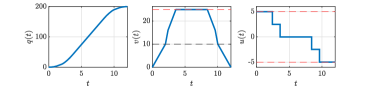
Figure 1: The position of the car $q(t)$ is shown in the left plot, the velocity $v(t)$ in the middle plot. Note the increase in acceleration in the turbo mode for $v>\bar{v}$. The right plots shows the optimal control $u(t)$.

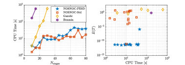
Figure 2: Comparison of NOSNOC to mixed integer formulations. The left plot show CPU time as function of number of control intervals ${N}_{\mathrm{stg}}$. The right plot show the solution accuracy as function of CPU time in a Pareto plot.

5.2 Numerical Benchmark

We solve the OCP from the last section with four different approaches. We use NOSNOC with the FESD discretization (12) and NOSNOC with the standard discretization (9). The latter approach is closely related to the smoothing approach in [8] and [9]. For the MPCC, we use in both cases the relaxation approach as it is usually the most robust one. Additionally, we make a big M reformulation of the PSS (15) and solve a mixed integer nonlinear program (MINLP). Switches are allowed only at the control interval boundaries, hence we have two binary variables per control interval. We solve the MINLP with the dedicated solver Bonmin [18]. Moreover, since the only non-linearity is in time $T$, we fix it and make a bisection-type search in $T$. For every fixed $T$ we solve a MILP with Gurobi. The MILP with the smallest $T$ that is still feasible delivers the optimal solution. We vary ${N}_{\mathrm{stg}}$ from 10 to 80 with steps of 5. The computations are aborted if the time-limit of 10 minutes is exceeded.

The results of the benchmark are depicted in Fig. 2. NOSNOC-FESD is slightly slower than NOSNOC-Std, since it has ${N}_{\mathrm{stg}}{N_{\mathrm{FE}}}$ more variables, as $h_{n}$ are degrees of freedom. We compare also the solution quality by making a high-accuracy simulation $x_{\mathrm{sim}}(t)$ of (15) with the obtained optimal controls $\mathbf{q}$. We compare the terminal constraint satisfaction $E(T)=\|x_{\mathrm{sim}}(T)-x_{\mathrm{goal}}\|$. Due to the exact switch detection property, NOSNOC-FESD has by far the most accurate solutions. The outlier where NOSNOC-Std achieves high accuracy corresponds to a local minima without switches. We see that even a simple nonsmooth OCP is difficult to solve with conventional approaches, whereas NOSNOC-FESD provides faster and several orders of magnitude more accurate solutions. Further detailed comparisons of FESD to the standard approach can be found in [2].

5.3 An Example with State Jumps and Time-Freezing

In this subsection we illustrate how to use NOSNOC with systems with state jumps. We consider a planar bouncing ball with elastic impacts. The state vector is defined as $x=(q,v)\in{\mathbb{R}}^{4}$ with $q=(q_{1},q_{2})\in{\mathbb{R}}^{2}$ and $v=(v_{1},v_{2})\in{\mathbb{R}}^{2}$ being the ball’s position and velocity, respectively. The initial state is $x(0)=(0,0.5,0,0)$ and the ball is controlled with some force $u\in{\mathbb{R}}^{2}$. The ODE with state jumps reads as:

$$\dot{q} =v,\;\dot{v}=u-(0,g),$$ (16a)

$$v_{2}(t^{+}) =-ev_{2}(t^{-}),\;\text{if}\;q_{2}(t)=0\ \text{and}\ v_{2}(t)<0.$$ (16b)

where $e\in\left(0,1\right]$ is the coefficient of restitution and determines the post impact velocity. The goal is to reach $q_{\mathrm{f}}=(4,0.5)$ with a minimal quadratic control effort modeled with the stage cost $f_{q}(x,u)=u^{\top}u$ and a minimal terminal velocity expressed via $f_{\mathrm{T}}(x)=100v^{\top}v$, with $T=4$. The control force is bounded such that it is weaker than the gravitational force, i.e., $u^{\top}u\leq u_{\mathrm{max}}^{2}$. The chosen parameters are $e=0.9$, $g=9.81$, $u_{\mathrm{max}}=9$. The following NOSNOC code solves the described nonsmooth OCP with state jump:

⬇

1[settings] = default_settings_fesd();

2settings.time_freezing = 1; settings.n_s = 3;

3model.T = 4; model.N_stg = 20; model.N_FE = 3;

4q = MX.sym(’q’,2); v = MX.sym(’v’,2);

5model.x = [q;v]; model.x0 = [0;0.5;0;0];

6u = MX.sym(’u’,2); model.u = u;

7model.c = q(2); model.e = 0.9;

8model.f = [v;u-[0;9.81]];

9model.f_q = u’*u; model.f_q_T = 100*v’*v;

10model.g_ineq = u’*u-9^2;

11model.g_terminal = q-[4;0.5];

12[results,stats,model,settings] = nosnoc_solver(model,settings);

The flag settings.time_freezing = 1 ensures that system with state jumps (16) is transformed into a PSS of the form of (1c) via the time-freezing reformulation [1]. A solution trajectory is given in Figure 3, note the state jumps in $v_{2}(t)$ in the middle plot.

Many more settings can be changed by the user, for example, one can choose between different MPCC reformulations via mpcc_mode, control the sparsity of the cross complementarities cross_complementarity_mode and so on. A few more examples and a detailed user manual are available NOSNOC’s repository [5].

6 Conclusion and Outlook

In this letter we presented NOSNOC, an open-source software package for nonsmooth numerical optimal control. With the help of the Finite Elements with Switch Detection (FESD) method and the time-freezing reformulation, it enables practical and high accuracy optimal control of several different classes of nonsmooth system in a unified way. The discretized OCP are solved with techniques solely from continuous optimization, without the need for any integer variables. All reformulations and details are hidden but accessible such that a convenient use for users with different knowledge levels of the field is ensured.

In future work, we aim to implement a python version of NOSNOC. Moreover, further algorithmic developments in FESD, e.g., different reformulations of PSS into DCS, support for time-freezing for other classes of hybrid systems will be implemented.

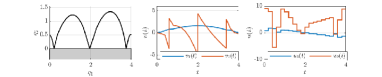
Figure 3: The illustration of the optimal solution $q(t)$ is shown in the left plot. The middle plot shows the optimal velocities $v(t)$ as a function of the physical time $t$, where the state jumps are recovered. The right plot shows the optimal controls $u(t)$.

References

- [1] A. Nurkanović, T. Sartor, S. Albrecht, and M. Diehl, “A Time-Freezing Approach for Numerical Optimal Control of Nonsmooth Differential Equations with State Jumps,” IEEE Control Systems Letters, vol. 5, no. 2, pp. 439–444, 2021.
- [2] A. Nurkanović, M. Sperl, S. Albrecht, and M. Diehl, “Finite Elements with Switch Detection for Direct Optimal Control of Nonsmooth Systems,” 2022. [Online]. Available: https://arxiv.org/abs/2205.05337
- [3] B. Brogliato and A. Tanwani, “Dynamical systems coupled with monotone set-valued operators: Formalisms, applications, well-posedness, and stability,” SIAM Review, vol. 62, no. 1, pp. 3–129, 2020.
- [4] A. Bemporad and M. Morari, “Control of systems integrating logic, dynamics, and constraints,” Automatica, vol. 35, no. 3, pp. 407–427, 1999.
- [5] “NOSNOC,” https://github.com/nurkanovic/nosnoc, 2022.
- [6] A. Nurkanović, S. Albrecht, B. Brogliato, and M. Diehl, “The Time-Freezing Reformulation for Numerical Optimal Control of Complementarity Lagrangian Systems with State Jumps,” arXiv preprint, 2021.
- [7] A. Nurkanović and M. Diehl, “Continuous optimization for control of hybrid systems with hysteresis via time-freezing,” Submitted to The IEEE Control Systems Letters (L-CSS), 2022.
- [8] D. E. Stewart and M. Anitescu, “Optimal control of systems with discontinuous differential equations,” Numerische Mathematik, vol. 114, no. 4, pp. 653–695, 2010.
- [9] A. Nurkanović, S. Albrecht, and M. Diehl, “Limits of MPCC Formulations in Direct Optimal Control with Nonsmooth Differential Equations,” in 2020 European Control Conference (ECC), 2020, pp. 2015–2020.
- [10] B. T. Baumrucker and L. T. Biegler, “MPEC strategies for optimization of a class of hybrid dynamic systems,” Journal of Process Control, vol. 19, no. 8, pp. 1248–1256, 2009.
- [11] S. Scholtes, “Convergence properties of a regularization scheme for mathematical programs with complementarity constraints,” SIAM Journal on Optimization, vol. 11, no. 4, pp. 918–936, 2001.
- [12] M. Anitescu, P. Tseng, and S. J. Wright, “Elastic-mode algorithms for mathematical programs with equilibrium constraints: global convergence and stationarity properties,” Mathematical Programming, vol. 110, no. 2, pp. 337–371, 2007.
- [13] J. A. E. Andersson, J. Gillis, G. Horn, J. B. Rawlings, and M. Diehl, “CasADi – a software framework for nonlinear optimization and optimal control,” Mathematical Programming Computation, vol. 11, no. 1, pp. 1–36, 2019.
- [14] A. Wächter and L. T. Biegler, “On the implementation of an interior-point filter line-search algorithm for large-scale nonlinear programming,” Mathematical Programming, vol. 106, no. 1, pp. 25–57, 2006.
- [15] D. E. Stewart, “A high accuracy method for solving ODEs with discontinuous right-hand side,” Numerische Mathematik, vol. 58, no. 1, pp. 299–328, 1990.
- [16] A. F. Filippov, Differential Equations with Discontinuous Righthand Sides. Springer Science & Business Media, Series: Mathematics and its Applications (MASS), 2013, vol. 18.
- [17] E. Hairer and G. Wanner, Solving Ordinary Differential Equations II – Stiff and Differential-Algebraic Problems, 2nd ed. Berlin Heidelberg: Springer, 1991.
- [18] P. Bonami, L. Biegler, A. Conn, G. Cornuéjols, I. Grossmann, C. Laird, J. Lee, A. Lodi, F. Margot, N. Sawaya, and A. Wächter, “An Algorithmic Framework For Convex Mixed Integer Nonlinear Programs,” IBM T. J. Watson Research Center, Tech. Rep., 2005.