New penalized criteria for smooth non-negative tensor factorization with missing entries

Abstract

Tensor factorization models are widely used in many applied fields such as chemometrics, psychometrics, computer vision or communication networks. Real life data collection is often subject to errors, resulting in missing data. Here we focus in understanding how this issue should be dealt with for non-negative tensor factorization. We investigate several criteria used for non-negative tensor factorization in the case where some entries are missing. In particular we show how smoothness penalties can compensate the presence of missing values in order to ensure the existence of an optimum. This lead us to propose new criteria with efficient numerical optimization algorithms. Numerical experiments are conducted to support our claims.

I Introduction

The ever growing literature on multi-way data has shown the effectiveness of tensor factorization models in many domains ranging from psychometrics and chemometrics to signal processing and machine learning (see [1, 2, 3] and the references therein). Key strengths of these models include 1) their flexibility in taking into account prior knowledge on the data such as non-negativity, sparsity or smoothness and 2) their ability to cope with missing data. As a result, they have proven very useful in real world applications, where factors are related to practical features. On the other hand, the theoretical study of tensor factorization is still a challenging research topic. In particular, finding the true factorization of a tensor is generally NP-Hard [4] and finding an approximated factorization requires solving a non-convex optimization problem often dealt with using an iterative algorithm based on alternating minimization or on gradient descent. Since the problem is non-convex, few guarantees exist on the convergence of the optimization method used except that the objective function decreases at each iteration and that the algorithm converges to a local minimum. A question which naturally arises in this context is the existence of a global minimum. Unfortunately, this existence is not always guaranteed and discrepancies have been explored in both theoretical and experimental works especially for the popular CANDECOMP/PARAFAC (CP) decomposition (see e.g. [5, 6] and the references therein). However, it is common knowledge in the inverse problem and statistical learning communities, that ill-posed problems can be handled by controlling the complexity of the solution space. This can be done, for example, using regularization [7, 8]. In the context of tensor factorization, is has been shown in [9, 6] that adding non-negativity constraints ensures existence of a global solution for the CP decomposition. This decomposition is known as non-negative tensor factorization (NTF). In this paper, we provide similar guarantees for the NTF problem in the case where some, possibly many, entries are missing. This case is of particular interest because missing data are very common in practical settings where the data collection can be subject to errors. Another interest of dealing with missing entries is that it allows to use cross validation methods to select hyperparameters such as penalty parameters or the tensor rank.

I-A Related work

The literature on tensor factorization from the past decades has given rise to a wide range of algorithms among which some are adapted to missing values and/or additional constraints. Methods handling missing values usually fall into one of the three following categories : imputation, weighted least squares and probabilistic models. In the first case, missing entries are estimated at each iteration resulting in an EM-like algorithm [10, 11]. In the second case the squared error is weighted with binary weights representing missing and observed entries (see e.g. [12, 13]). In the last case, prior distributions are proposed for the factors and their parameters are estimated from the observed data [14, 15, 16]. The problem of missing entries is also closely related to tensor completion where, in addition to the factors, one usually also tries to estimate a full tensor which coincides with the data tensor on observed entries (see e.g [17] for a recent survey). Because of the need for efficient algorithms to deal with large amount of data, the literature on tensor factorization is dominated by algorithmic considerations, especially when missing values are taken into account.

The effect of using smoothness constraints or penalties has also been thoroughly explored both for tensor factorization and tensor completion [18, 19, 20, 21, 22, 23, 24, 25]. Such approaches are generally used for numerical purposes to regularize ill-posed optimization problems and for statistical purposes to compensate overfitting by incorporating prior knowledge or assumption on the model. This can be beneficial for the interpretation of the factors [18, 19, 26, 25] but also for the accuracy of the factorization or completion. For example, total variation constraints are widely used to deal with natural images as they are able to capture their smoothness structure [27, 28, 22]. There are two main strategies to impose smoothness on the factors. The first strategy, which is studied in this paper, consists in adding a penalty term in the loss. Usual penalties for smoothness involve the total variation norm or the $L^{2}$ norm of the second derivative for spline smoothing, [19, 28, 22, 26, 25]. The second strategy consists in representing the factors within specific lower dimensional spaces, using splines, polynomials or kernels [18, 19, 29, 20, 21, 30, 23, 24, 31].

I-B Notation

The interval of integers between $i$ and $j$ is denoted by ${\left\llbracket i,j\right\rrbracket}:=\{i,\cdots,j\}$. We use bold capital letters to denote tensors and matrices and bold lowercase letters for vectors. Standard font is used for the entries of the tensors, matrices and vectors. For example, ${\bf A}=[{\bf a}_{1},\cdots,{\bf a}_{R}]\in\mathbb{R}^{I\times R}$ means that ${\bf a}_{r}\in\mathbb{R}^{I}$ is the $r$-th column of ${\bf A}$ and the $(i,r)$-th entry of ${\bf A}$ is denoted by $A_{i,r}$ or $a_{i,r}$. A tensor ${\bf X}\in\mathbb{R}^{I_{1}\times\cdots\times I_{N}}$ is indexed by a vector of integers $\mathbf{i}=i_{1:n}:=(i_{1},\cdots,i_{N})\in\prod_{n=1}^{N}{\left\llbracket 1,I_{n}\right\rrbracket}$ and we write $X_{\mathbf{i}}=X_{i_{1},\cdots,i_{n}}$. We denote the outer product between vectors by $\circ$ and the Hadamard product between tensors by $\oast$. We refer to [1] for the definitions of these usual tensor operations. We recall that the Frobenius scalar product of two tensors ${\bf X},{\bf Y}\in\mathbb{R}^{I_{1}\times\cdots\times I_{N}}$ is defined as $\left\langle{\bf X},{\bf Y}\right\rangle_{F}=\sum_{\mathbf{i}}X_{\mathbf{i}}Y_{\mathbf{i}}$ and we denote by ${\left\|\cdot\right\|}_{F}$ its induced norm. The total variation $p$-norm of a vector ${\bf a}\in\mathbb{R}^{I}$ is ${\left\|{\bf a}\right\|}_{{\rm TV},p}=\left(\sum_{i=1}^{I-1}\left|a_{i}-a_{i+1}\right|^{p}\right)^{1/p}$ for $p\in[1,\infty)$ and ${\left\|{\bf a}\right\|}_{{\rm TV},\infty}=\max_{1\leq i\leq I-1}\left|a_{i}-a_{i+1}\right|$. For a given norm or semi-norm $\nu$ on $\mathbb{R}^{I}$ we respectively denote $\mathbb{S}_{\nu}^{+}:=\left\{{\bf a}\in\mathbb{R}_{+}^{I}\,:\;\nu({\bf a})=1\right\}$ and $\mathbb{B}^{+}_{\nu}:=\left\{{\bf a}\in\mathbb{R}_{+}^{I}\,:\;\nu({\bf a})\leq 1\right\}$ the unit positive sphere and the unit positive ball. We also write for any spaces $\mathcal{X}_{1},\cdots,\mathcal{X}_{N}$, $x^{(1:N)}:=(x^{(1)},\cdots,x^{(N)})\in\prod_{n=1}^{N}\mathcal{X}_{n}$. Finally, throughout this paper we will denote the $N$ dimensional grid of indices by $\mathcal{I}=\prod_{n=1}^{N}{\left\llbracket 1,I_{n}\right\rrbracket}$ and, for any tensor ${\bf X}\in\mathbb{R}^{I_{1},\cdots,I_{N}}$ and any set $A\subset\mathbb{R}$, we denote the set of indices at which ${\bf X}$’s entries fall into $A$ by $\{{\bf X}\in A\}$. Specifically, we denote $\{{\bf X}=x\}=\{{\bf X}\in\{x\}\}$ the set of indices with entries equal to $x$ or $\{{\bf X}>x\}=\{{\bf X}\in{\left(x,+\infty\right)}\}$.

The remaining of this paper is organized as follows. In Section II, we describe the tensor factorization problem and introduce two losses and their related optimization algorithms. The main theoretical contributions are gathered in Section III. Numerical experiments are conducted in Section IV for comparing the optimization algorithms of Section II. Proofs are postponed to Section VI.

II Losses and optimization algorithms

A tensor ${\bf Y}\in\mathbb{R}^{I_{1}\times\cdots\times I_{N}}$ is said to admit a non-negative tensor factorization with rank $R$ if there exists a sequence of $N$ factor matrices ${\bf A}^{(1:N)}\in\prod_{n=1}^{N}\mathbb{R}_{+}^{I_{1}\times R}$ such that

$${\bf Y}=\sum_{r=1}^{R}{\bf a}_{r}^{(1)}\circ\cdots\circ{\bf a}_{r}^{(N)}\;,$$ (1)

where we recall that ${\bf a}_{r}^{(n)}$ is the $r$-th column of ${\bf A}^{(n)}$. In order to avoid scaling indeterminacy in the tensor factorization, it is common to use an equivalent formulation of (1) using normalized factors based on $N$ norms $\nu_{1},\cdots,\nu_{N}$ on $\mathbb{R}^{I_{1}},\cdots,\mathbb{R}^{I_{N}}$. Let us set, for all $n\in{\left\llbracket 1,N\right\rrbracket}$ and $r\in{\left\llbracket 1,R\right\rrbracket}$, $\lambda_{r}=\prod_{n=1}^{n}\nu_{n}({\bf a}_{r}^{(n)})$ and $\tilde{{\bf a}}_{r}^{(n)}=\frac{{\bf a}_{r}^{(n)}}{\nu_{n}({\bf a}_{r}^{(n)})}$ if $\nu_{n}({\bf a}_{r}^{(n)})>0$ and any arbitrary element of $\mathbb{S}_{\nu_{n}}^{+}$ otherwise. Then, the factorization (1) can be written as

$${\bf Y}=\sum_{r=1}^{R}\lambda_{r}\tilde{{\bf a}}_{r}^{(1)}\circ\cdots\circ\tilde{{\bf a}}_{r}^{(N)}\;.$$ (2)

We study the problem of approximating a tensor ${\bf X}\in\mathbb{R}^{I_{1}\times\cdots\times I_{N}}$ by a finite rank tensor using parameterization (1) or (2) in the case where some entries of the tensor are missing. Let ${\bf W}\in\mathbb{R}_{+}^{I_{1},\cdots,I_{N}}$ be a tensor of weights and define

$$L_{\bf W}({\bf A}):={\left\|{\bf W}\oast\left({\bf X}-\sum_{r=1}^{R}{\bf a}_{r}^{(1)}\circ\cdots\circ{\bf a}_{r}^{(N)}\right)\right\|}_{F}^{2}\;,$$

for all ${\bf A}={\bf A}^{(1:N)}\in\prod_{n=1}^{N}\mathbb{R}_{+}^{I_{n}\times R}$. We also define the normalized equivalent,

$$\tilde{L}_{{\bf W}}(\boldsymbol{\lambda},\tilde{{\bf A}}):={\left\|{\bf W}\oast\left({\bf X}-\sum_{r=1}^{R}\lambda_{r}\tilde{{\bf a}}_{r}^{(1)}\circ\cdots\circ\tilde{{\bf a}}_{r}^{(N)}\right)\right\|}_{F}^{2}\;,$$

for all $\boldsymbol{\lambda}\in\mathbb{R}_{+}^{R}$ and $\tilde{{\bf A}}=\tilde{{\bf A}}^{(1:N)}\in\prod_{n=1}^{N}\left(\mathbb{S}_{\nu_{n}}^{+}\right)^{R}$, where we view $\left(\mathbb{S}_{\nu_{n}}^{+}\right)^{R}$ as the set of matrices in $\mathbb{R}_{+}^{I_{n}\times R}$ whose columns are valued in $\mathbb{S}_{\nu_{n}}^{+}$. In this framework, it is implicitly assumed that the zero entries of ${\bf W}$ indicate missing entries and ${\bf W}$ is usually taken as a binary tensor.

We also introduce two penalties based on $N$ semi-norms $\mu_{1},\cdots,\mu_{N}$ defined on $\mathbb{R}^{I_{1}},\cdots,\mathbb{R}^{I_{N}}$ respectively. Namely, given two integers $d,p$ with $d\geq p\geq 1$ and $\boldsymbol{\alpha}\in\mathbb{R}_{+}^{N}$, we define, for all $\boldsymbol{\lambda}\in\mathbb{R}_{+}^{R}$ and $\tilde{{\bf A}}=\tilde{{\bf A}}^{(1:N)}\in\prod_{n=1}^{N}\left(\mathbb{S}_{\nu_{n}}^{+}\right)^{R}$,

$$\tilde{\mathcal{P}}_{\boldsymbol{\alpha}}(\boldsymbol{\lambda},\tilde{\bf A}):=\sum_{n=1}^{N}\alpha_{n}\sum_{r=1}^{R}\lambda_{r}^{d}\,\mu_{n}^{p}(\tilde{\bf a}_{r}^{(n)})\;,$$ (3)

where we use the notation $\mu_{n}^{p}({\bf a})=\left(\mu_{n}({\bf a})\right)^{p}$. This includes the penalty of [28] by taking $d=2$ and $\mu_{n}={\left\|\cdot\right\|}_{{\rm TV},p}$ for $p=1,2$. We propose a new penalty, defined as the unnormalized equivalent of (3), which reads as

$$\mathcal{P}_{\boldsymbol{\alpha}}({\bf A}):=\sum_{n=1}^{N}\alpha_{n}\sum_{r=1}^{R}\nu_{n}^{d-p}({\bf a}_{r}^{(n)})\,\mu_{n}^{p}({\bf a}_{r}^{(n)})\,\prod_{m\neq n}\nu_{m}^{d}({\bf a}_{r}^{(m)})\;,$$ (4)

for all ${\bf A}={\bf A}^{(1:N)}\in\prod_{n=1}^{N}\mathbb{R}_{+}^{I_{n}\times R}$.

Then, let $f_{{\bf W},\boldsymbol{\alpha}}:=L_{\bf W}+\mathcal{P}_{\boldsymbol{\alpha}}$ and $\tilde{f}_{{\bf W},\boldsymbol{\alpha}}:=\tilde{L}_{\bf W}+\tilde{\mathcal{P}}_{\boldsymbol{\alpha}}$ and consider the two following equivalent optimization problems

$$\begin{split}&\min_{{\bf A}^{(1:N)}}f_{{\bf W},\boldsymbol{\alpha}}({\bf A}^{(1:N)})\\ &\text{s.t. }\forall n\in{\left\llbracket 1,N\right\rrbracket},\,{\bf A}^{(n)}\in\mathbb{R}_{+}^{I_{n}\times R}\;,\end{split}$$ (5)

and

$$\begin{split}&\min_{\boldsymbol{\lambda},\tilde{\bf A}^{(1:N)}}\tilde{f}_{{\bf W},\boldsymbol{\alpha}}(\boldsymbol{\lambda},\tilde{{\bf A}}^{(1:N)})\\ &\text{s.t. }\forall r\in{\left\llbracket 1,R\right\rrbracket},\lambda_{r}\geq 0\text{ and }\forall n\in{\left\llbracket 1,N\right\rrbracket},\tilde{\bf a}_{r}^{(n)}\in\mathbb{S}_{\nu_{n}}^{+}\;.\end{split}$$ (6)

The fact that the $\tilde{{\bf a}}_{r}^{(n)}$’s are constrained individually in Problem (6) naturally leads to the Hierarchical Alternating Least Squares (HALS) optimization method (see e.g. [2, 28]). This method consists in minimizing $\tilde{f}_{{\bf W},\boldsymbol{\alpha}}$ alternatively in the $\tilde{{\bf a}}_{r}^{(n)}$’s and its updates are recalled in Algorithm 1 where we have defined ${\bf X}^{(r)}:={\bf X}-\sum_{s\neq r}\lambda_{s}\tilde{{\bf a}}_{s}^{(1)}\circ\cdots\circ\tilde{{\bf a}}_{s}^{(N)}$ and $\tilde{f}_{{\bf W},\boldsymbol{\alpha}}^{(r,n)}(\tilde{{\bf a}}):={\left\|{\bf W}\oast({\bf X}^{(r)}-\lambda_{r}\tilde{{\bf a}}_{r}^{(1)}\circ\cdots\tilde{{\bf a}}_{r}^{(n-1)}\circ\tilde{{\bf a}}\circ\tilde{{\bf a}}_{r}^{(n+1)}\circ\cdots\circ\tilde{{\bf a}}_{r}^{(N)})\right\|}_{F}^{2}$ $+\alpha_{n}\lambda_{r}^{d}\mu_{n}^{p}(\tilde{{\bf a}})$.

Data: ${\bf X}$, ${\bf W}$ and initial values for $\boldsymbol{\lambda},\tilde{{\bf A}}^{(1)},\cdots,\tilde{{\bf A}}^{(N)}$

${\bf E}={\bf X}-\sum_{r=1}^{R}\lambda_{r}\tilde{{\bf a}}_{r}^{(1)}\circ\cdots\circ\tilde{{\bf a}}_{r}^{(N)}$

repeat

       for $r=1,\cdots,R$ do

             ${\bf X}^{(r)}={\bf E}+\lambda_{r}\tilde{{\bf a}}_{r}^{(1)}\circ\cdots\circ\tilde{{\bf a}}_{r}^{(N)}$

             for $n=1,\cdots,N$ do

                   $\displaystyle\tilde{{\bf a}}_{r}^{(n)}=\mathop{\mathrm{argmin}}_{\tilde{{\bf a}}\in\mathbb{S}_{\nu_{n}}^{+}}\tilde{f}_{{\bf W},\boldsymbol{\alpha}}^{(r,n)}(\tilde{{\bf a}})$

             end for

            $\displaystyle\lambda_{r}=\mathop{\mathrm{argmin}}_{\lambda\geq 0}{\left\|{\bf W}\oast({\bf X}^{(r)}-\lambda\tilde{{\bf a}}_{r}^{(1)}\circ\cdots\circ\tilde{{\bf a}}_{r}^{(N)})\right\|}_{F}^{2}$

             ${\bf E}={\bf X}^{(r)}-\lambda_{r}\tilde{{\bf a}}_{r}^{(1)}\circ\cdots\circ\tilde{{\bf a}}_{r}^{(N)}$

       end for

      

until Change of value of $\tilde{f}_{{\bf W},\alpha}$ is sufficiently small;

return $\boldsymbol{\lambda},\tilde{{\bf A}}^{(1)},\cdots,\tilde{{\bf A}}^{(N)}$

Algorithm 1 HALS algorithm

The update for $\tilde{{\bf a}}_{r}^{(n)}$ in Algorithm 1 requires minimizing the function $\tilde{f}_{{\bf W},\boldsymbol{\alpha}}^{(r,n)}$ on the non-negative sphere $\mathbb{S}_{\nu_{n}}^{+}$. In the case where there is no non-negativity constraint, [28] proposes to use a projected gradient method. In our case, we propose to first solve $\min_{\tilde{{\bf a}}\in\mathbb{R}_{+}^{I_{n}}}\tilde{f}_{{\bf W},\boldsymbol{\alpha}}^{(r,n)}(\tilde{{\bf a}})$ using a gradient-based method with bound constraints such as L-BFGS-B and then normalize the result by its $\nu_{n}$-norm. The update in $\lambda_{r}$ writes as $\lambda_{r}=\left[\frac{\left\langle{\bf W}\oast{\bf X}^{(r)},{\bf W}\oast(\tilde{\bf a}_{r}^{(1)}\circ\cdots\circ\tilde{\bf a}_{r}^{(N)})\right\rangle_{F}}{{\left\|{\bf W}\oast(\tilde{\bf a}_{r}^{(1)}\circ\cdots\circ\tilde{\bf a}_{r}^{(N)})\right\|}_{F}^{2}}\right]_{+}$.

On the other hand, the constraints in Problem (5) reduce to a bound constraint on a vectorization of ${\bf A}$. Hence, in the case where the gradients of $\mu_{n}$ and $\nu_{n}$ are available, we can follow the approach of [13] and use a gradient-based method with bound constraints such as L-BFGS-B.

In the next section, we study the existence of a global optimum for Problem (6). The existence of a global optimum for Problem (5) follows immediately as they are two different parameterizations of the same criterion. However, using the normalized version allows for stronger results, such as coercivity, which are not possible in the unnormalized version as already noted in [6].

III Existence of a global optimum for the weighted NTF

In this section, we consider the normalized version of the weighed NTF problem, i.e. Problem (6), where, for all $n\in{\left\llbracket 1,N\right\rrbracket}$, $\nu_{n}$ is a norm on $\mathbb{R}^{I_{n}}$ and $\mu_{n}$ is a semi-norm on $\mathbb{R}^{I_{n}}$. To simplify the presentation, we set $\Theta:=\mathbb{R}_{+}^{R}\times\prod_{n=1}^{N}\left(\mathbb{S}_{\nu_{n}}^{+}\right)^{R}$ and $\boldsymbol{\theta}=(\boldsymbol{\lambda},{\bf A}^{(1:N)})\in\Theta$. We investigate the existence of a minimum with minimal assumptions on the semi-norms used in the penalty term. Namely, for $n=1,\dots,N$, we define

$$\psi_{n}:=\sup\left\{\nu_{n}({\bf a})\,:\;{\bf a}\in\mathbb{B}^{+}_{\mu_{n}}\right\}\;,$$ (7)

$$\psi_{n}^{\prime}:=\sup\left\{\nu_{n}({\bf a})\,:\;{\bf a}\in\mathbb{B}^{+}_{\mu_{n}},\exists i\in{\left\llbracket 1,I_{n}\right\rrbracket}\,,a_{i}=0\right\}\;,$$ (8)

and consider the following admissibility condition for the semi-norm $\mu_{n}$.

1. We have $\psi_{n}^{\prime}<\psi_{n}=\infty$,

Condition $\psi_{n}=\infty$ simply says that $\mu_{n}$ is not a norm on the positive cone (otherwise it would be equivalent to the norm $\nu_{n}$). The condition $\psi_{n}^{\prime}<\infty$ says that $\mu_{n}$ behaves as a norm on the positive sub-cone that have at least one zero entry. Condition (AC) holds for semi-norms typically used in smoothness penalties, as shown by the following lemma.

Lemma III.1.

Condition (AC) holds for $\mu_{n}$ defined as one of the following semi-norms.

1. For all ${\bf a}\in\mathbb{R}^{I_{n}}$, $\mu_{n}({\bf a})={\left\|{\bf a}\right\|}_{{\rm TV},p}$ for some $p\in[1,+\infty]$.

2. For all ${\bf a}\in\mathbb{R}^{I_{n}}$, $\mu_{n}({\bf a})=\left(\int_{0}^{1}(a^{\prime\prime}(u))^{2}\,\mathrm{d}u\right)^{1/2}$, where $a:[0,1]\to\mathbb{R}$ is the natural cubic spline such that, for all $i\in{\left\llbracket 1,I_{n}\right\rrbracket}$, $a(u_{i})=a_{i}$ for some $0<u_{1}\leq\cdots\leq u_{I_{n}}<1$.

In the next theorem, we provide a necessary and sufficient condition for $\tilde{f}_{{\bf W},\boldsymbol{\alpha}}$ to be coercive on $\Theta$, which means that $\tilde{f}_{{\bf W},\boldsymbol{\alpha}}(\theta)$ tends to $+\infty$ as the norm of $\theta$ goes to $+\infty$.

The necessary and sufficient condition relies on the following definition of cylinders.

Definition III.1.

For any non-empty subset $\mathcal{N}\subset{\left\llbracket 1,N\right\rrbracket}$, a $\mathcal{N}$-cylinder is a set defined as

$$\mathcal{C}((j_{n})_{n\in\mathcal{N}}):=\left\{\mathbf{i}\in\mathcal{I}\,:\;i_{n}=j_{n},\;\forall n\in\mathcal{N}\right\}\;,$$ (9)

for some $(j_{n})_{n\in\mathcal{N}}\in\prod_{n\in\mathcal{N}}{\left\llbracket 1,I_{n}\right\rrbracket}$. In particular, the whole set $\mathcal{I}$ the unique $\emptyset$-cylinder.

Then the following result holds.

Theorem III.2.

Let $\boldsymbol{\alpha}\in\mathbb{R}_{+}^{N}$ and suppose that, for all $n\in\{\boldsymbol{\alpha}>0\}$, $\mu_{n}$ satisfies (AC). Then the two following assertions are equivalent.

1. The set $\{{\bf W}=0\}$ contains no $\{\boldsymbol{\alpha}=0\}$-cylinder.

2. The function $\tilde{f}_{{\bf W},\boldsymbol{\alpha}}$ is coercive on $\Theta$.

In this case, both $\tilde{f}_{{\bf W},\boldsymbol{\alpha}}$ and $f_{{\bf W},\boldsymbol{\alpha}}$ admit global minima on $\Theta$ and on $\prod_{n=1}^{N}\mathbb{R}_{+}^{I_{n}\times R}$, respectively.

We assume that $\mu_{n}$ satisfy (AC) only for $n\in\{\boldsymbol{\alpha}>0\}$ because, for $n\in\{\boldsymbol{\alpha}=0\}$, $\mu_{n}$ vanishes in the penalty (3). Also note that Assertion (i) means that no $\{\boldsymbol{\alpha}=0\}$-cylinder is missing and is not very restrictive. For example, if all modes are penalized, i.e. $\{\boldsymbol{\alpha}=0\}=\emptyset$, then Assertion (i) does not hold if and only if all entries are missing. In the experiments, we study the case of color image completion where $N=3$ and the first two modes correspond to pixels and the third corresponds to the color channel. In this case, we penalize only the first two modes, i.e. $\{\boldsymbol{\alpha}=0\}=\{3\}$. This means that Assertion (i) does not hold if and only if an entire color channel is missing.

IV Experimental results

In this section, we compare the two optimization problems (5) and (6) with the penalties defined in (3) and (4) respectively where we take $p=d=2$. The first optimization problem is solved using the scipy implementation of L-BFSG-B. The second optimization problem is solved using Algorithm 1. We propose two experiments. In the first one, we try to recover factors from an incomplete and noisy observation of a tensor of the type (2) with $N=3$. In the second one, we apply the algorithms for color image completion. In both experiments and each of the algorithm, we take $\boldsymbol{\alpha}=[\alpha,\alpha,0]^{\top}$ where $\alpha>0$, and $\nu_{n}={\left\|\cdot\right\|}_{2}$ for all $n$. The maximum number of iterations is set to $10^{4}$ and the iterations are stopped if the relative improvement of the loss is lower than $10^{-6}$. One iteration of the HALS algorithm consists of the steps in the repeat–until box of Algorithm 1 and one iteration of the L-BFSG-B method consists in one update of the gradient descent. In this case, during one iteration, all the factors are updated. The computational performances algorithms are compared using the average computing time per iteration denoted by TPI. All the experiments are run on a Linux Workstation with 40 Intel Xeon E5-2630 v4 2.20 GHz processors.

IV-A Factor estimation on toy data

In this experiment, we construct a tensor ${\bf X}={\bf Y}+\sigma{\bf E}\in\mathbb{R}^{I\times I\times I}$ where ${\bf Y}$ is as in (2) with $I=50$, $N=3$ and $R=5$ and ${\bf E}$ has a standard normal entries. The factors ${\bf a}_{r}^{(3)}$ are sampled uniformly on $[0,1]$ and the factors ${\bf a}_{r}^{(1)}$ and ${\bf a}_{r}^{(2)}$ are constructed by taking non-negative random linear combination of $7$ B-Spline functions of order $4$. With this construction, the factors are non-negative and smooth for $n=1,2$ and we allow the ${\bf a}_{r}^{(2)}$’s to vanish on some intervals (see the first column of Figure 3). The standard deviation $\sigma>0$ is computed as in [12, 13], i.e. $\sigma=(100/\nu-1)^{-1/2}\frac{{\left\|{\bf Y}\right\|}_{F}}{{\left\|{\bf E}\right\|}_{F}}$, and we take $\nu=10$. Since the true factors are generated from B-splines, we take $\mu_{n}$ as in (ii) of Lemma III.1. We generated $25\%,50\%$ and $70\%$ percent of missing data which are drawn randomly and uniformly on the grid ${\left\llbracket 1,I\right\rrbracket}^{3}$. For the unnormalized problem, we use an SVD-based initialization and use its normalized equivalent for the normalized problem. To evaluate the output $\hat{{\bf Y}}=\sum_{r=1}^{R}\hat{\lambda}_{r}\hat{\bf a}_{r}^{(1)}\circ\hat{\bf a}_{r}^{(2)}\circ\hat{\bf a}_{r}^{(3)}$, we use the normalized mean square error, NMSE $=\frac{{\left\|{\bf Y}-\hat{{\bf Y}}\right\|}_{F}^{2}}{{\left\|{\bf Y}\right\|}_{F}^{2}}$ and the similarity score, SIM $=\max_{\sigma\in\mathscr{S}_{R}}\frac{1}{R}\sum_{r=1}^{R}\prod_{n=1}^{N}\left\langle\tilde{{\bf a}}_{r}^{(n)},\hat{\bf a}_{\sigma(r)}^{(n)}\right\rangle$, where $\mathscr{S}_{R}$ denotes the set of permutations of ${\left\llbracket 1,R\right\rrbracket}$. Note that, since the $\tilde{{\bf a}}_{r}^{(n)}$’s and $\hat{{\bf a}}_{r}^{(n)}$’s have unit $2$-norm, we have SIM $\in[0,1]$. A lower NSME is interpreted as a better prediction of $Y$’s entries while a higher SIM is interpreted as a better estimation of its factors. An example of reconstruction is shown in Figure 3 where we observe that the gradient method is able to reconstruct the factors even when the proportion of missing data is high. In the remaining of this section, we discuss the choice of $\alpha$ and compare the methods with various values of $I$.

IV-A1 Data-driven selection of $\alpha$

We propose to evaluate the selection of $\alpha$ using a $5$-fold cross validation criterion (CV), which amounts to arbitrarily introduce additional missing values in the objective function and evaluate their prediction errors. More precisely, we generate randomly $5$ binary masks $({\bf W}_{k})_{k\in{\left\llbracket 1,5\right\rrbracket}}$ such that the sets $\left(\{{\bf W}_{k}>0\}\right)_{k\in{\left\llbracket 1,5\right\rrbracket}}$ create a partition of $\mathcal{I}$. For each fold $k\in{\left\llbracket 1,5\right\rrbracket}$ and each value of $\alpha\in\{0,10^{-4},10^{-3},10^{-2},10^{-1},1,10\}$, we minimize $f_{{\bf W}\oast{\bf W}_{k},\boldsymbol{\alpha}}$ (or $\tilde{f}_{{\bf W}\oast{\bf W}_{k},\boldsymbol{\alpha}}$) and the cross validation score is computed using $f_{{\bf W}\oast({\bf 1}-{\bf W}_{k}),\boldsymbol{\alpha}}$ (or $\tilde{f}_{{\bf W}\oast({\bf 1}-{\bf W}_{k}),\boldsymbol{\alpha}}$), where ${\bf 1}$ is the tensor with all entries equal to $1$. We compare the cross validation scores with an oracle selection of $\alpha$ given by the NMSE and SIM scores which use the ground truth. The results are gathered in Figure 1 where we observe that the selection with the cross validation score seems consistent with the oracle based on NMSE, which indicates that CV is a suitable parameter selection method in our context. Note that the oracle selection using the SIM score can give different optimal values for $\alpha$. This can be explained by the fact that the SIM score is more sensitive to small differences between the estimated factors and the true factors.

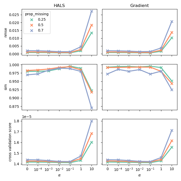
Figure 1: CV selection of $\alpha$ (bottom), compared to the SIM (middle) and NMSE (top) critera.

IV-A2 Comparison with various dimensions

We now compare the proposed methods for various values of $I$. We use the same ground truth represented by the first column of Figure 3 where we interpolated the factors to achieve higher values of $I$. The comparison is made in a best case scenario where, for each value of $I$, each proportion of missing data and each model, we use the oracle selection of $\alpha\in\{0,10^{-4},10^{-3},10^{-2},10^{-1},1,10\}$ based on the NMSE score. The NMSE and SIM scores and the TPI are gathered in Figure 2. The two methods give very similar results for the NMSE and SIM whose values indicate almost perfect reconstruction in all cases. We observe that the reconstruction tends to be better for large values of $I$ which is expected since the difficulty of the problem decreases as $I$ increases (see [13]). The advantage of the gradient-based method is, however, highlighted by the TPI, especially when the dimension increases. Note that we observed that the value of $\alpha$ does not affect much the TPI and therefore the comparison displayed in Figure 2 is representative of any value of $\alpha$.

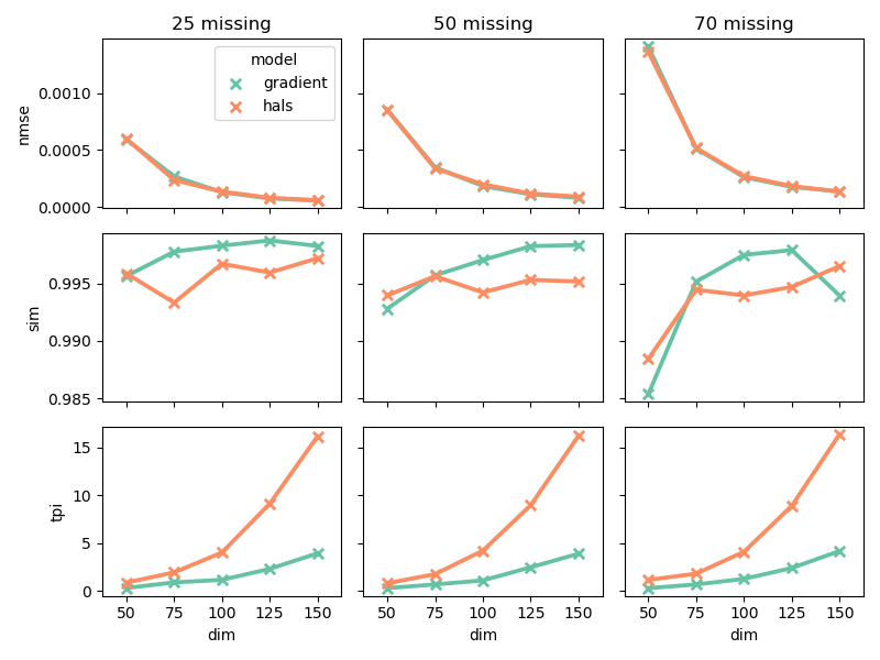
Figure 2: Best case scenario for different dimensions.

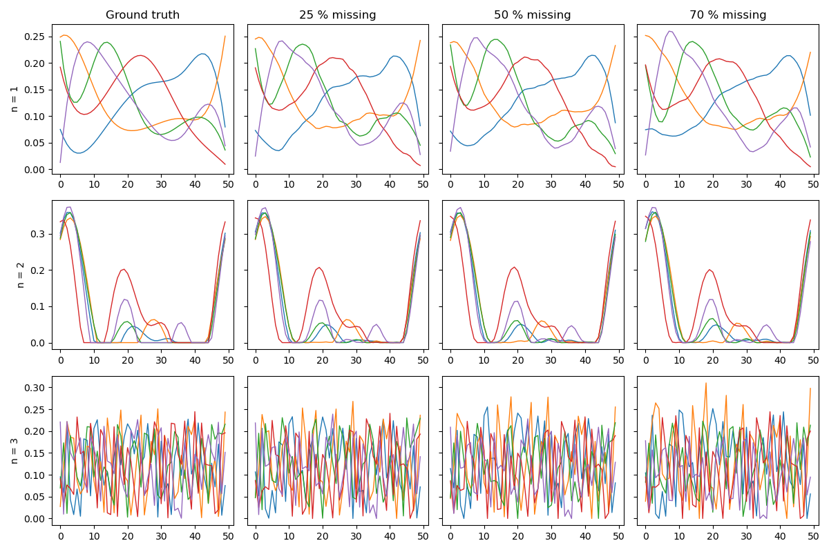
Figure 3: Estimated factors with gradient-based method and $\alpha=0.1$. Rows represent the modes (i.e. $n$) and colors represent the components (i.e. $r$).

IV-B Color image completion

In this experiment, we apply both methods to $3$ color images (barbara, baboon and giant) of size $256\times 256\times 3$. Missing data are generated in two ways. In the first case, we remove all the color channels for $80\%$ of the pixels selected randomly and uniformly. In the last case, we remove all the color channels for a mask obtained by scribbling the image. Note that, in all of these cases, Assertion (i) of Theorem III.2 holds. We use the quadratic variation penalty as in [28], i.e. $\mu_{n}={\left\|\cdot\right\|}_{{\rm TV},2}$. The quality of completion, is evaluated by the peak signal-to-noise ratio (PSNR) and structural similarity index (SSIM) as in [28]. High PSNR and SSIM indicate a good completion. For both methods, we take a fix rank $R=50$ and use a random initialization. For each image, each mask and each model, we use the oracle selection of $\alpha$ based on the SSIM. As observed in Figure 4, there is an optimal value of $\alpha$ which should neither be too small nor too large. This value is not necessarily the same for both algorithms. We also observe that, near the optimal value of $\alpha$, the gradient-based method gives a better SSIM score than the HALS method. This is also highlighted by the completed images displayed in Figure 5. Note also that the gradient-based method has much lower TPI than the HALS one.

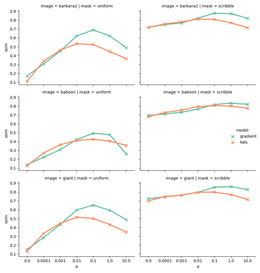
Figure 4: Evolution of the SSIM with $\alpha$. Rows represent the three images and columns represent the types of mask.

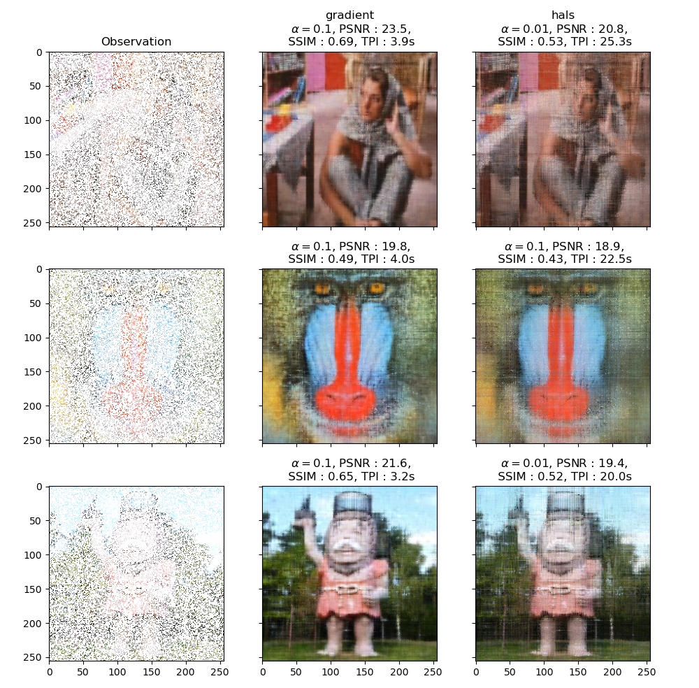
(a) Uniformly missing pixels.

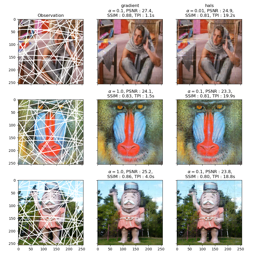
(b) Masked pixels.

Figure 5: Image completion comparison with $\alpha$ giving the best SSIM.

V Conclusion

In this contribution, we extended previous results on the existence of a global minimum for the non-negative tensor factorization problem to the case where some entries are missing. We showed that, under non-restrictive assumptions on the observed entries, adding a penalty to the quadratic loss ensures the existence of a global minimum. We proposed two formulations of the problem: a normalized one, which is solved using a HALS algorithm, and an unnormalized one, which is solved using a gradient-based method. The experimental study illustrates the advantages of the gradient-based method in computing time and in reconstruction error.

VI Proofs

VI-A Preliminary results

In this section, we provide preliminary results which are necessary to prove Theorem III.2. To simplify the notation, let us define, for all $\boldsymbol{\theta}=(\boldsymbol{\lambda},{\bf A}^{(1:N)})\in\Theta:=\mathbb{R}_{+}^{R}\times\prod_{n=1}^{N}\left(\mathbb{S}_{\nu_{n}}^{+}\right)^{R}$,

$$g_{\bf W}(\boldsymbol{\theta}):={\left\|{\bf W}\oast\left(\sum_{r=1}^{R}\lambda_{r}{\bf a}_{r}^{(1)}\circ\cdots\circ{\bf a}_{r}^{(N)}\right)\right\|}_{F}\;,$$ (10)

and, for all ${\bf a}^{(1:N)}\in\prod_{n=1}^{N}\mathbb{S}_{\nu_{n}}^{+}$,

$$h_{{\bf W}}({\bf a}^{(1:N)}):={\left\|{\bf W}\oast\left({\bf a}^{(1)}\circ\cdots\circ{\bf a}^{(N)}\right)\right\|}_{F}^{2}\;.$$ (11)

Then the following proposition holds.

Proposition VI.1.

Let $\mathcal{A}=\prod_{n=1}^{N}\mathcal{A}_{n}^{R}$ be such that for all $n\in{\left\llbracket 1,N\right\rrbracket}$, $\mathcal{A}_{n}\subset\mathbb{S}_{\nu_{n}}^{+}$. Denote by $\overline{\mathcal{A}_{n}}$ the closure of $\mathcal{A}_{n}$ in $\mathbb{S}_{\nu_{n}}^{+}$. Then the three following assertions are equivalent.

1. The function $\tilde{L}_{\bf W}$ is coercive on $\mathbb{R}_{+}^{R}\times\mathcal{A}$.

2. The function $g_{\bf W}$ is coercive on $\mathbb{R}_{+}^{R}\times\mathcal{A}$.

3. For all ${\bf a}^{(1:N)}\in\prod_{n=1}^{N}\overline{\mathcal{A}_{n}}$, there exists $\mathbf{i}\in\{{\bf W}>0\}$ such that $\prod_{n=1}^{N}{\bf a}_{i_{n}}^{(n)}>0$.

Proof.

The equivalence between (i) and (ii) is a direct consequence of the two triangular inequalities. Now, note that, by continuity of $h_{\bf W}$, Assertion (iii) is equivalent to

$$\inf\left\{h_{\bf W}({\bf a}^{(1:N)})\,:\;{\bf a}^{(1:N)}\in\prod_{n=1}^{N}\mathcal{A}_{n}\right\}>0\;.$$ (12)

Hence, it remains to prove that (ii) and (12) are equivalent.

Proof of (12) $\Rightarrow$ (ii). Assume that Condition (12) holds and let $(\boldsymbol{\theta}(m))_{m\in\mathbb{N}}\in\left(\mathbb{R}_{+}^{R}\times\mathcal{A}\right){N}$ with ${\left\|\boldsymbol{\theta}(m)\right\|}_{2}\xrightarrow[m\to+\infty]{}+\infty$ and, for all $m\in\mathbb{N}$, $\boldsymbol{\theta}(m)=(\boldsymbol{\lambda}(m),{\bf A}^{(1:N)}(m))$. Then, since $\mathcal{A}$ is bounded, we must have ${\left\|\boldsymbol{\lambda}(m)\right\|}_{2}\xrightarrow[m\to+\infty]{}+\infty$ and, using the fact that the entries of $\boldsymbol{\theta}(m)$ are all non-negative, we get

$$\left(g_{{\bf W}}(\boldsymbol{\theta}(m))\right)^{2} \geq\sum_{r=1}^{R}\left(\lambda_{r}(m)\right)^{2}h_{{\bf W}}({\bf a}_{r}^{(1:N)}(m))$$

$$\geq c_{\inf}{\left\|\boldsymbol{\lambda}(m)\right\|}_{2}^{2}\;,$$

where $c_{\inf}$ is the inf in (12). Hence, under Condition (12), $g_{{\bf W}}(\boldsymbol{\theta}(m))$ diverges to $+\infty$ as $m\to+\infty$ and Assertion (ii) follows.

Proof of (ii) $\Rightarrow$ (12). Assume that Condition (12) does not hold and let us show that $\tilde{g}_{{\bf W}}$ is not coercive on $\mathbb{R}_{+}^{R}\times\mathcal{A}$ by constructing a sequence $(\boldsymbol{\theta}(m))_{m\in\mathbb{N}}\in\left(\mathbb{R}_{+}^{R}\times\mathcal{A}\right){N}$ such that ${\left\|\boldsymbol{\theta}(m)\right\|}\xrightarrow[m\to+\infty]{}+\infty$ and $g_{\bf W}(\boldsymbol{\theta}(m))\xrightarrow[m\to+\infty]{}0$. Let us set, for all $m\in\mathbb{N}$, $\boldsymbol{\theta}(m):=(\boldsymbol{\lambda}(m),{\bf A}^{(1:N)}(m))$ with $\boldsymbol{\lambda}(m)=[m,0,\cdots,0]$ and, for all $n\in\mathbb{N}$, ${\bf A}^{(n)}(m)=[{\bf a}^{(n)}(m),{\bf a}_{2}^{(n)},\cdots,{\bf a}_{R}^{(n)}]$, where ${\bf a}_{2}^{(n)},\cdots,{\bf a}_{R}^{(n)}$ are any elements of $\mathcal{A}_{n}$ and ${\bf a}^{(1:N)}(m)\in\prod_{n=1}^{N}\mathcal{A}_{n}$ is such that $h_{\bf W}({\bf a}^{(1:N)}(m))\leq 2^{-m}$. Note that such ${\bf a}^{(1:N)}(m)$ exists because Condition (12) does not hold. With this construction, we get ${\left\|\boldsymbol{\theta}(m)\right\|}\xrightarrow[m\to+\infty]{}+\infty$ and $\left(g_{\bf W}(\boldsymbol{\theta}(m))\right)^{2}=m^{2}h_{\bf W}({\bf a}^{(1:N)}(m))\leq m^{2}2^{-m}\xrightarrow[m\to+\infty]{}0$, which concludes the proof. ∎

For the second result, we consider specific subsets

$$\mathcal{A}_{n}({\boldsymbol{\rho}},C):=\left\{{\bf a}\in\mathbb{S}_{\nu_{n}}^{+}\,:\;\mu_{n}({\bf a})\leq\rho_{n}C\right\}\;,$$ (13)

$$\Theta({\boldsymbol{\rho}},C):=\mathbb{R}_{+}^{R}\times\prod_{n=1}^{N}\left(\mathcal{A}_{n}({\boldsymbol{\rho}},C)\right)^{R}\;,$$ (14)

where $C\geq 0$ and ${\boldsymbol{\rho}}\in{\left(0,+\infty\right]}^{N}$. Note that, for all $n$ such that $\rho_{n}=+\infty$, we have $\mathcal{A}_{n}({\boldsymbol{\rho}},C)=\mathbb{S}_{\nu_{n}}^{+}$. Let us define

$$C_{\bf W}({\boldsymbol{\rho}}):=\inf\left\{C\geq 0\,:\;\begin{tabular}[]{l}$\tilde{L}_{{\bf W}}$ is not coercive\\ on $\Theta({\boldsymbol{\rho}},C)$\end{tabular}\right\}\;.$$ (15)

The goal of the remaining of this section it to derive an explicit formulation of $C_{\bf W}({\boldsymbol{\rho}})$. To this end, we need to introduce the following sets and constants. For any $n\in{\left\llbracket 1,N\right\rrbracket}$ and $\mathcal{J}\subset{\left\llbracket 1,I_{n}\right\rrbracket}$, define

$$\mathcal{A}_{n}(\mathcal{J}):=\left\{{\bf a}\in\mathbb{S}_{\nu_{n}}^{+}\,:\;\forall j\in\mathcal{J},a_{j}=0\right\}\;,$$

$$m_{n}(\mathcal{J}):=\inf\left\{\mu_{n}({\bf a})\,:\;{\bf a}\in\mathcal{A}_{n}(\mathcal{J})\right\}\;,$$

with the convention $\inf(\emptyset)=+\infty$. Moreover, for any $\mathcal{I}^{\prime}\subset\mathcal{I}$ and $n\in{\left\llbracket 1,N\right\rrbracket}$, we define the projection of $\mathcal{I}^{\prime}$ onto the $n$-th coordinate as $\pi_{n}(\mathcal{I}^{\prime}):=\left\{i_{n}\,:\;\mathbf{i}\in\mathcal{I}^{\prime}\right\}$ and denote by

$$\mathscr{J}(\mathcal{I}^{\prime}):=\left\{\mathcal{J}_{1:N}\,:\;\begin{split}&\forall n\in{\left\llbracket 1,N\right\rrbracket}\,,\,\mathcal{J}_{n}\subseteq\pi_{n}(\mathcal{I}^{\prime})\,,\\ &\forall\mathbf{i}\in\mathcal{I}^{\prime}\,,\,\exists n\in{\left\llbracket 1,N\right\rrbracket},i_{n}\in\mathcal{J}_{n}\end{split}\right\}$$

the class of sequences of sets $\mathcal{J}_{1:N}=(\mathcal{J}_{1},\cdots,\mathcal{J}_{N})$, where each $\mathcal{J}_{n}$ is a subset of all the $n$-th entries of the vector indices in $\mathcal{I}^{\prime}$ and such that each vector index $\mathbf{i}$ in $\mathcal{I}^{\prime}$ has at least one entry, say the $n$-th, present in the corresponding $\mathcal{J}_{n}$.

Finally, we define, for all ${\boldsymbol{\rho}}\in{\left(0,+\infty\right]}^{N}$ and $\mathcal{I}^{\prime}\subset\mathcal{I}$,

$$C({\boldsymbol{\rho}},\mathcal{I}^{\prime}):=\min\left\{c({\boldsymbol{\rho}},\mathcal{J}_{1:N})\,:\;\mathcal{J}_{1:N}\in\mathscr{J}(\mathcal{I}^{\prime})\right\}\;,$$ (16)

where

$$c({\boldsymbol{\rho}},\mathcal{J}_{1:N}):=\begin{cases}\infty&\text{if $\exists n\,,\,\mathcal{A}_{n}(\mathcal{J}_{n})=\emptyset$,}\\ \displaystyle\max_{n\in{\left\llbracket 1,N\right\rrbracket}}\frac{m_{n}(\mathcal{J}_{n})}{\rho_{n}}&\text{otherwise.}\end{cases}$$

The first case in the definition of $c({\boldsymbol{\rho}},\mathcal{J}_{1:N})$ amounts to use the convention $\inf(\emptyset)/\rho=+\infty$ for any $\rho\in(0,\infty]$. We have the following results.

Lemma VI.2.

Let $n\in{\left\llbracket 1,N\right\rrbracket}$, and $\mathcal{J}\subset{\left\llbracket 1,I_{n}\right\rrbracket}$, the following assertions hold.

1. We have $m_{n}(\mathcal{J})=+\infty$ if and only if $\mathcal{J}={\left\llbracket 1,I_{n}\right\rrbracket}$.

2. If $\mu_{n}$ satisfies (AC), we have $m_{n}(\mathcal{J})=0$ if and only if $\mathcal{J}=\emptyset$.

Proof.

Assertion (i) follows from the equivalence between $m_{n}(\mathcal{J})=+\infty$ and $\mathcal{A}_{n}(\mathcal{J})=\emptyset$, which is itself equivalent to $\mathcal{J}={\left\llbracket 1,I_{n}\right\rrbracket}$. For Assertion (ii), recall that $\psi_{n}=\infty$ means that $\mu_{n}$ is a semi-norm which is not a norm on the positive cone, which implies $m_{n}(\emptyset)=0$ thus showing the “if” implication. For the “only if” implication, note that $m_{n}(\mathcal{J})>0$ if and only if

$$\sup\left\{\nu_{n}({\bf a})\,:\;{\bf a}\in\mathbb{B}^{+}_{\mu_{n}}({\bf a})_{,},\,\forall j\in\mathcal{J}\,,\,{\bf a}_{j}=0\right\}<\infty\;.$$

Hence, if $\psi^{\prime}_{n}<\infty$, this happens whenever $\mathcal{J}\neq\emptyset$. ∎

Lemma VI.3.

Let $\mathcal{I}^{\prime}\subset\mathcal{I}$ and ${\boldsymbol{\rho}}\in(0,+\infty]^{N}$. Then the following assertions hold.

1. We have $C({\boldsymbol{\rho}},\mathcal{I}^{\prime})=+\infty$ if and only if $\mathcal{I}^{\prime}=\mathcal{I}$.

2. If $\mu_{n}$ satisfies (AC) for all $n\in\{{\boldsymbol{\rho}}<+\infty\}$, then $C({\boldsymbol{\rho}},\mathcal{I}^{\prime})>0$ if and only if $\mathcal{I}\setminus\mathcal{I}^{\prime}$ contains no $\{{\boldsymbol{\rho}}=+\infty\}$-cylinder.

Proof.

Using Assertion (i) of Lemma VI.2, we get that

$$C ({\boldsymbol{\rho}},\mathcal{I}^{\prime})<+\infty$$

$$\Leftrightarrow\exists\,\mathcal{J}_{1:N}\in\mathscr{J}(\mathcal{I}^{\prime}),\forall n\in{\left\llbracket 1,N\right\rrbracket},m_{n}(\mathcal{J}_{n})<+\infty$$

$$\Leftrightarrow\exists\,\mathcal{J}_{1:N}\in\mathscr{J}(\mathcal{I}^{\prime}),\forall n\in{\left\llbracket 1,N\right\rrbracket},\mathcal{J}_{n}\neq{\left\llbracket 1,I_{n}\right\rrbracket}$$

$$\Leftrightarrow\exists\,\mathcal{J}_{1:N}\in\mathscr{J}(\mathcal{I}^{\prime}),\exists\mathbf{i}\in\mathcal{I},\forall n\in{\left\llbracket 1,N\right\rrbracket},i_{n}\notin\mathcal{J}_{n}$$

$$\Leftrightarrow\mathscr{J}(\mathcal{I}^{\prime})\cap(\mathscr{J}(\mathcal{I}))^{c}\neq\emptyset\;.$$

Hence, to conclude the proof of Assertion (i), we need to show that $\mathscr{J}(\mathcal{I}^{\prime})\cap(\mathscr{J}(\mathcal{I}))^{c}\neq\emptyset$ if and only if $\mathcal{I}^{\prime}\neq\mathcal{I}$. The “only if” implication is straightforward by contraposition. For the “if” implication, assume that $\mathcal{I}^{\prime}\neq\mathcal{I}$ and take $\mathbf{i}\in\mathcal{I}\setminus\mathcal{I}^{\prime}$. Then it is easily seen that, taking $\mathcal{J}_{n}=\pi_{n}(\mathcal{I}^{\prime})\setminus\{i_{n}\}$ for all $n\in{\left\llbracket 1,N\right\rrbracket}$, we get $\mathcal{J}_{1:N}\in\mathscr{J}(\mathcal{I}^{\prime})\cap(\mathscr{J}(\mathcal{I}))^{c}$ which is therefore non-empty. This concludes the proof of Assertion (i).

For Assertion (ii), note that $C({\boldsymbol{\rho}},\mathcal{I}^{\prime})=0$ is equivalent to

$$\exists\,\mathcal{J}_{1:N}\in\mathscr{J}(\mathcal{I}^{\prime}),\,\forall n\in{\left\llbracket 1,N\right\rrbracket},\,{\boldsymbol{\rho}}_{n}^{-1}m_{n}(\mathcal{J}_{n})=0\;,$$

which, by Lemma VI.2 and (AC), is in turn equivalent to

$$\exists\,\mathcal{J}_{1:N}\in\mathscr{J}(\mathcal{I}^{\prime}),\,\begin{cases}\forall n\in\{{\boldsymbol{\rho}}=+\infty\},\,\mathcal{J}_{n}\neq{\left\llbracket 1,I_{n}\right\rrbracket}\;,\\ \forall n\in\{{\boldsymbol{\rho}}<+\infty\},\,\mathcal{J}_{n}=\emptyset\;.\\ \end{cases}$$ (17)

We now prove that (17) holds if and only if there exists $(j_{n})_{n\in\{{\boldsymbol{\rho}}=+\infty\}}\in\prod_{n\in\{{\boldsymbol{\rho}}=+\infty\}}{\left\llbracket 1,I_{n}\right\rrbracket}$ such that $\mathcal{C}((j_{n})_{n\in\{{\boldsymbol{\rho}}=+\infty\}})\subset\mathcal{I}\setminus\mathcal{I}^{\prime}$. First, assume that (17) holds and take $j_{n}\in{\left\llbracket 1,I_{n}\right\rrbracket}\setminus\{\mathcal{J}_{n}\}$ for all $n\in\{{\boldsymbol{\rho}}=+\infty\}$. Assume that $\mathcal{C}((j_{n})_{n\in\{{\boldsymbol{\rho}}=+\infty\}})\not\subset\mathcal{I}\setminus\mathcal{I}^{\prime}$. This means that there exists $\mathbf{i}\in\mathcal{C}((j_{n})_{n\in\{{\boldsymbol{\rho}}=+\infty\}})\cap\mathcal{I}^{\prime}$. Then, by definition of $\mathscr{J}(\mathcal{I}^{\prime})$, there exists $n\in\{{\boldsymbol{\rho}}=+\infty\}$ such that $j_{n}=i_{n}\in\mathcal{J}_{n}$ which contradicts the fact that $j_{n}\in{\left\llbracket 1,I_{n}\right\rrbracket}\setminus\{\mathcal{J}_{n}\}$. Hence $\mathcal{C}((j_{n})_{n\in\{{\boldsymbol{\rho}}=+\infty\}})\subset\mathcal{I}\setminus\mathcal{I}^{\prime}$ thus proving the “only if” implication. For the “if” implication, assume that there exists $(j_{n})_{n\in\{{\boldsymbol{\rho}}=+\infty\}}\in\prod_{n\in\{{\boldsymbol{\rho}}=+\infty\}}{\left\llbracket 1,I_{n}\right\rrbracket}$ such that $\mathcal{C}((j_{n})_{n\in\{{\boldsymbol{\rho}}=+\infty\}})\subset\mathcal{I}\setminus\mathcal{I}^{\prime}$. Then, we get (17) by taking $\mathcal{J}_{n}=\emptyset$ for $n\in\{{\boldsymbol{\rho}}<+\infty\}$ and $\mathcal{J}_{n}={\left\llbracket 1,I_{n}\right\rrbracket}\setminus\{j_{n}\}$ for $n\in\{{\boldsymbol{\rho}}=+\infty\}$. ∎

Lemma VI.4.

For all ${\boldsymbol{\rho}}\in{\left(0,+\infty\right]}^{N}$, we have

$$C_{\bf W}({\boldsymbol{\rho}})=C({\boldsymbol{\rho}},\{{\bf W}>0\})\;,$$ (18)

Proof.

The proof relies on the identity

$$c({\boldsymbol{\rho}},\mathcal{J}_{1:N})=\\ \inf\left\{\max_{n\in{\left\llbracket 1,N\right\rrbracket}}\rho_{n}^{-1}\mu_{n}({\bf a}^{(n)})\,:\;\forall n,{\bf a}^{(n)}\in\mathcal{A}_{n}(\mathcal{J}_{n})\right\}\;.$$ (19)

To prove (19), first note that, if there exists $n\in{\left\llbracket 1,I_{n}\right\rrbracket}$, such that $\mathcal{J}_{n}={\left\llbracket 1,I_{n}\right\rrbracket}$, then the two terms of (19) are equal to $+\infty$. We now assume that, for all $n\in{\left\llbracket 1,I_{n}\right\rrbracket}$, $\mathcal{J}_{n}\neq{\left\llbracket 1,I_{n}\right\rrbracket}$. Then the inequality $\leq$ of (19) is a straightforward consequence of the definition of $c({\boldsymbol{\rho}},\mathcal{J}_{1:N})$. Let us now show that there exists ${\bf a}^{(1:N)}\in\prod_{n=1}^{N}\mathcal{A}_{n}(\mathcal{J}_{n})$ such that $c({\boldsymbol{\rho}},\mathcal{J}_{1:N})=\max_{n\in{\left\llbracket 1,N\right\rrbracket}}\rho_{n}^{-1}\mu_{n}({\bf a}^{(n)})$. It suffices to take, for $n\in{\left\llbracket 1,N\right\rrbracket}$, ${\bf a}^{(n)}\in\mathcal{A}_{n}(\mathcal{J}_{n})$ such that $\mu_{n}({\bf a}^{(n)})=m_{n}(\mathcal{J}_{n})$. Such ${\bf a}^{(n)}$ exists because $\mathcal{A}_{n}(\mathcal{J}_{n})$ is compact and $\mu_{n}$ is continuous. This concludes the proof of (19).

Now, to prove (18), we show that, for all $C\geq 0$, $\tilde{L}_{\bf W}$ is not coercive on $\Theta({\boldsymbol{\rho}},C)$ if and only if $C\geq C({\boldsymbol{\rho}},\{{\bf W}>0\})$. For the “only if” implication, assume that $C$ is such that $\tilde{L}_{\bf W}$ is not coercive on $\Theta({\boldsymbol{\rho}},C)$. Then, from Proposition VI.1 and closeness of the $\mathcal{A}_{n}({\boldsymbol{\rho}},C)$’s defined in (13), we get that there exists ${\bf a}^{(1:N)}\in\prod_{n=1}^{N}\mathcal{A}_{n}({\boldsymbol{\rho}},C)$ such that, for all $\mathbf{i}\in\{{\bf W}>0\}$, there exists $n\in{\left\llbracket 1,N\right\rrbracket}$ such that $a_{i_{n}}^{(n)}=0$. Using this observation, we construct $\mathcal{J}_{1:N}\in\mathscr{J}(\{{\bf W}>0\})$ by the following procedure. Start with $\mathcal{J}_{n}=\emptyset$ for all $n\in{\left\llbracket 1,N\right\rrbracket}$ and then, for each $\mathbf{i}\in\{{\bf W}>0\}$, select one of the $n$’s such that $a_{i_{n}}^{(n)}=0$ and put $i_{n}$ in $\mathcal{J}_{n}$. With this construction, we have ${\bf a}^{(1:N)}\in\prod_{n=1}^{N}\mathcal{A}_{n}(\mathcal{J}_{n})\cap\mathcal{A}_{n}({\boldsymbol{\rho}},C)$ and therefore

$$C\geq\max_{n\in{\left\llbracket 1,N\right\rrbracket}}\rho_{n}^{-1}\mu_{n}({\bf a}^{(n)})\geq c({\boldsymbol{\rho}},\mathcal{J}_{1:N})\geq C({\boldsymbol{\rho}},\{{\bf W}>0\})\;,$$

where the first inequality comes from (13), the second from (19) and the last from (16).

For the “if” implication, let us take $C\geq C({\boldsymbol{\rho}},\{{\bf W}>0\})$ and show that Assertion (iii) of Proposition VI.1 does not hold. Note that we can take ${\bf W}$ such that $\{{\bf W}>0\}\neq\mathcal{I}$ because the other case is straightforward. Then, by definition of $C({\boldsymbol{\rho}},\{{\bf W}>0\})$, we know that there exists $\mathcal{J}_{1:N}\in\mathscr{J}(\{{\bf W}>0\})$ such that $C({\boldsymbol{\rho}},\{{\bf W}>0\})=c({\boldsymbol{\rho}},\mathcal{J}_{1:N})$. Moreover, since $\{{\bf W}>0\}\neq\mathcal{I}$, Assertion (i) of Lemma VI.2 gives that $c({\boldsymbol{\rho}},\mathcal{J}_{1:N})<+\infty$ and therefore we are in the case where the infimum in (19) is reached. Hence there exists ${\bf a}^{(1:N)}\in\prod_{n=1}^{N}\mathcal{A}_{n}(\mathcal{J}_{n})$ such that $\max_{n\in{\left\llbracket 1,N\right\rrbracket}}\rho_{n}^{-1}\mu_{n}({\bf a}^{(n)})=C({\boldsymbol{\rho}},\{{\bf W}>0\})$. This gives that, for all $n\in{\left\llbracket 1,N\right\rrbracket}$, $\mu_{n}({\bf a}^{(n)})\leq\rho_{n}C({\boldsymbol{\rho}},\{{\bf W}>0\})\leq\rho_{n}C$ and therefore ${\bf a}^{(n)}\in\mathcal{A}_{n}({\boldsymbol{\rho}},C)$, as defined in (13). On the other hand, $\mathcal{J}_{1:N}\in\mathscr{J}(\{{\bf W}>0\})$ means that, for all $\mathbf{i}\in\{{\bf W}>0\}$, there exists $n\in{\left\llbracket 1,N\right\rrbracket}$ such that $i_{n}\in\mathcal{J}_{n}$ and we get that ${\bf a}_{i_{n}}^{(n)}=0$ because ${\bf a}^{(n)}\in\mathcal{A}_{n}(\mathcal{J}_{n})$. Hence Assertion (iii) of Proposition VI.1 does not hold and the proof is concluded. ∎

VI-B Proofs of Theorem III.2 and Lemma III.1

Proof of Theorem III.2.

In the proof, we use the functions $g_{\bf W}$ and $h_{\bf W}$ defined respectively in (10) and (11). Note that, as in Proposition VI.1, we have that $\tilde{f}_{{\bf W},\boldsymbol{\alpha}}$ is coercive on $\Theta$ if and only if $g_{\bf W}^{2}+\tilde{\mathcal{P}}_{\boldsymbol{\alpha}}$ is coercive on $\Theta$.

Proof of (i) $\Rightarrow$ (ii). Assume that (i) holds and let us show that $g_{\bf W}^{2}+\tilde{\mathcal{P}}_{\boldsymbol{\alpha}}$ is coercive on $\Theta$. Take $\boldsymbol{\theta}=(\boldsymbol{\lambda},{\bf A}^{(1:N)})\in\Theta$ and let $s\in{\left\llbracket 1,R\right\rrbracket}$ be such that $\lambda_{s}=\max_{r\in{\left\llbracket 1,R\right\rrbracket}}\lambda_{r}={\left\|\boldsymbol{\lambda}\right\|}_{\infty}$. Then, since all the entries of $\boldsymbol{\theta}$ are non-negative, we have

$$(g_{\bf W} (\boldsymbol{\theta}))^{2}+\tilde{\mathcal{P}}_{\boldsymbol{\alpha}}(\boldsymbol{\theta})$$

$$\geq(\lambda_{s}^{2}\wedge\lambda_{s}^{d})\left(h_{{\bf W}}({\bf a}_{s}^{(1:N)})+\sum_{n=1}^{N}\alpha_{n}\mu_{n}^{p}({\bf a}_{s}^{(n)}))\right)$$

$$\geq\left[{\left\|\boldsymbol{\lambda}\right\|}_{\infty}^{d\wedge 2}-1\right]_{+}\eta\;,$$

where

$$\eta:=\inf_{{\bf a}^{(1:N)}\in\prod_{n=1}^{N}\mathbb{S}_{\nu_{n}}^{+}}\left(h_{\bf W}({\bf a}^{(1:N)})+\sum_{n=1}^{N}\alpha_{n}\mu_{n}^{p}({\bf a}^{(n)})\right)\;.$$

Hence, to prove that $g_{\bf W}^{2}+\tilde{\mathcal{P}}_{\boldsymbol{\alpha}}$ is coercive on $\Theta$, it suffices to prove that $\eta>0$. Now let us set, for all $n\in{\left\llbracket 1,N\right\rrbracket}$, $\rho_{n}=\alpha_{n}^{-p}$ with the convention that $0^{-p}=+\infty$. Then, Lemma VI.4 and Assertion (ii) of Lemma VI.3 give that $C_{\bf W}({\boldsymbol{\rho}})>0$. Take $0<C<C_{{\bf W}}({\boldsymbol{\rho}})$ and set $\mathcal{A}:=\prod_{n=1}^{N}\mathcal{A}_{n}({\boldsymbol{\rho}},C)$ with $\mathcal{A}_{n}({\boldsymbol{\rho}},C)$ defined as in (13). Then, by definition of $C_{\bf W}({\boldsymbol{\rho}})$ in (15) and Relation (12), we have $\inf_{\mathcal{A}}h_{\bf W}>0$. Moreover, for all ${\bf a}^{(1:N)}\in\mathcal{A}^{c}$, there exists $k\in{\left\llbracket 1,N\right\rrbracket}$ such that ${\bf a}^{(k)}\notin\mathcal{A}_{k}({\boldsymbol{\rho}},C)$, i.e. $\alpha_{k}\mu^{p}({\bf a}_{r}^{(k)})>C^{p}$ and $\sum_{n=1}^{N}\alpha_{n}\mu_{n}^{p}({\bf a}^{(n)})\geq\alpha_{k}\mu_{n}^{p}({\bf a}_{r}^{(k)})>C^{p}$. Hence, we get $h_{\bf W}+\sum_{n=1}^{N}\alpha_{n}\mu_{n}^{p}\geq\left(\inf_{\mathcal{A}}h_{\bf W}\right)\mathbbm{1}_{\mathcal{A}}+C^{p}\mathbbm{1}_{\mathcal{A}^{c}}$ so that $\eta\geq\left(\inf_{\mathcal{A}}h_{\bf W}\right)\wedge C^{p}>0$, thus concluding the proof.

Proof of (ii) $\Rightarrow$ (i). Let us assume that (i) does not hold and show that $g_{\bf w}^{2}+\tilde{\mathcal{P}}_{\boldsymbol{\alpha}}$ is not coercive on $\Theta$ by constructing a sequence $(\boldsymbol{\theta}(m))_{m\in\mathbb{N}}\in\Theta{N}$ such that $\boldsymbol{\theta}(m)\xrightarrow[m\to+\infty]{}+\infty$ and $g_{\bf W}^{2}(\boldsymbol{\theta}(m))+\tilde{\mathcal{P}}_{\boldsymbol{\alpha}}(\boldsymbol{\theta}(m))\xrightarrow[m\to+\infty]{}0$. We set, for all $n\in{\left\llbracket 1,N\right\rrbracket}$, $\rho_{n}=\alpha_{n}^{-p}$ with the convention that $0^{-p}=+\infty$. Then, from Assertion (ii) of Lemma VI.3, we get that $C_{\bf W}({\boldsymbol{\rho}})=0$. By definition of $C_{\bf W}({\boldsymbol{\rho}})$ and Relation (12), this gives that for all $m\in\mathbb{N}$, $\inf_{\mathcal{A}^{(m)}}h_{\bf W}=0$ with $\mathcal{A}^{(m)}=\prod_{n=1}^{N}\mathcal{A}_{n}({\boldsymbol{\rho}},2^{-m/p})$. In particular, we can find ${\bf a}^{(1:N)}(m)\in\mathcal{A}^{(m)}$ such that $h_{\bf W}({\bf a}^{(1:N)}(m))\leq 2^{-m}$. Now, take, for all $m\in\mathbb{N}$, $\boldsymbol{\theta}(m)=(\boldsymbol{\lambda}(m),{\bf A}^{(1:N)})$ with $\boldsymbol{\lambda}(m)=[m,0,\cdots,0]$ and, for all $n\in{\left\llbracket 1,N\right\rrbracket}$, ${\bf A}^{(n)}(m)=[{\bf a}^{(n)}(m),{\bf a}_{2}^{(n)},\cdots,{\bf a}_{R}^{(n)}]$, where ${\bf a}_{2}^{(n)},\cdots,{\bf a}_{R}^{(n)}$ are arbitrary elements of $\mathbb{S}_{\nu_{n}}^{+}$. In this case, we have ${\left\|\boldsymbol{\theta}(m)\right\|}_{2}\xrightarrow[m\to+\infty]{}+\infty$, but $\left(g_{\bf W}(\boldsymbol{\theta}(m))\right)^{2}+\tilde{\mathcal{P}}_{\boldsymbol{\alpha}}(\boldsymbol{\theta}(m))\leq(m^{2}+Nm^{d})2^{-m}\xrightarrow[m\to+\infty]{}0$, which concludes the proof. ∎

Proof of Lemma III.1.

The fact that none of the $\mu_{n}$’s in Points (i) and (ii) is a norm on the positive cone proves that $\psi_{n}=\infty$ in both cases. We now show that $\psi^{\prime}_{n}<\infty$ holds in both cases. By equivalence of the norms, we can assume without loss of generality that $\nu_{n}={\left\|\cdot\right\|}_{\infty}$. For $\mu_{n}$ as in Case (i), we can take $p=1$ without loss of generality. Then, for all $i,j\in{\left\llbracket 1,I_{n}\right\rrbracket}$, we have $\left|a_{j}-a_{i}\right|\leq\sum_{k=j\wedge i}^{j\vee i-1}\left|a_{k+1}-a_{k}\right|\leq{\left\|{\bf a}\right\|}_{{\rm TV},1}$. This implies $\psi^{\prime}_{n}<\infty$. Next, we take $\mu_{n}$ as in Case (ii). Let ${\bf a}\in\mathbb{B}^{+}_{n}$ such that $a_{j}=0$ for some $j\in{\left\llbracket 1,I_{n}\right\rrbracket}$. Let $(\hat{a}_{k})_{k\in\mathbb{Z}}$ be the Fourier coefficients of the corresponding Spline function $a$, $\hat{a}_{k}=\int_{0}^{1}a(u)\,\mathrm{e}^{-2\mathrm{i}\pi ku}\;\mathrm{d}u$. Then, we have $\mu_{n}({\bf a})=\left(\sum_{k\in\mathbb{Z}}\left|\hat{a}_{k}\right|^{2}(2\pi k)^{2}\right)^{1/2}\leq 1$. Now, using the Cauchy-Schwarz inequality and the fact that $1/12=\sum_{k\in\mathbb{Z}^{*}}(2\pi k)^{-2}$, where $\mathbb{Z}^{*}$ is the set of non-zero relative integers, we get that

$$\sum_{k\in\mathbb{Z}^{*}}\left|\hat{a}_{k}\right|\leq\left(\sum_{k\in\mathbb{Z}^{*}}(2\pi k)^{-2}\right)^{1/2}\mu_{n}({\bf a})\leq\frac{1}{2\sqrt{3}}\;.$$

In particular, we get $\sum_{k\in\mathbb{Z}}\left|\hat{a}_{k}\right|<+\infty$ and therefore, for all $u\in[0,1]$, we have $a(u)=\sum_{k\in\mathbb{Z}}\hat{a}_{k}\mathrm{e}^{2\mathrm{i}\pi ku}$. This implies that

$${\left\|{\bf a}\right\|}_{\infty} ={\left\|{\bf a}-a_{j}\right\|}_{\infty}$$

$$\leq\sup_{u\in[0,1]}\left|a(u)-a(u_{j})\right|$$

$$\leq\sum_{k\in\mathbb{Z}^{*}}\left|\hat{a}_{k}\right|\sup_{u\in[0,1]}\left|\mathrm{e}^{2\mathrm{i}\pi ku}-\mathrm{e}^{2\mathrm{i}\pi ku_{j}}\right|$$

$$\leq 2\sum_{k\in\mathbb{Z}^{*}}\left|\hat{a}_{k}\right|\;.$$

Hence, with the previous inequality, $\psi^{\prime}_{n}\leq\frac{1}{\sqrt{3}}$ in this case, which concludes the proof. ∎

References

• [1] T. G. Kolda and B. W. Bader, “Tensor decompositions and applications,” SIAM Review, vol. 51, no. 3, pp. 455–500, September 2009.
• [2] A. Cichocki, R. Zdunek, A. H. Phan, and S. Amari, Nonnegative Matrix and Tensor Factorizations: Applications to Exploratory Multi-Way Data Analysis and Blind Source Separation.   Wiley Publishing, 2009.
• [3] N. D. Sidiropoulos, L. De Lathauwer, X. Fu, K. Huang, E. E. Papalexakis, and C. Faloutsos, “Tensor decomposition for signal processing and machine learning,” IEEE Transactions on Signal Processing, vol. 65, no. 13, pp. 3551–3582, 2017.
• [4] C. J. Hillar and L.-H. Lim, “Most tensor problems are np-hard,” J. Acm, vol. 60, no. 6, Nov. 2013. [Online]. Available: https://doi.org/10.1145/2512329
• [5] V. de Silva and L.-H. Lim, “Tensor rank and the ill-posedness of the best low-rank approximation problem,” SIAM J. Matrix Anal. Appl., vol. 30, no. 3, pp. 1084–1127, 2008. [Online]. Available: https://doi.org/10.1137/06066518X
• [6] L.-H. Lim and P. Comon, “Nonnegative approximations of nonnegative tensors,” Journal of Chemometrics, vol. 23, no. 7‐8, pp. 432–441, 2009. [Online]. Available: https://onlinelibrary.wiley.com/doi/abs/10.1002/cem.1244
• [7] A. N. Tikhonov and V. Y. Arsenin, Solutions of ill-posed problems, ser. Scripta Series in Mathematics.   V. H. Winston & Sons, Washington, D.C.: John Wiley & Sons, New York-Toronto, Ont.-London, 1977, translated from the Russian, Preface by translation editor Fritz John.
• [8] V. N. Vapnik, Statistical learning theory, ser. Adaptive and Learning Systems for Signal Processing, Communications, and Control.   John Wiley & Sons, Inc., New York, 1998, a Wiley-Interscience Publication.
• [9] L.-H. Lim, “Optimal solutions to non-negative parafac/multilinear nmf always exist,” in Workshop on Tensor Decompositions and Applications, Centre International de rencontres Mathématiques, Luminy, France, 2005.
• [10] R. Bro, “Parafac. tutorial and applications,” Chemometrics and Intelligent Laboratory Systems, vol. 38, no. 2, pp. 149–171, 1997. [Online]. Available: https://www.sciencedirect.com/science/article/pii/S0169743997000324
• [11] C. A. Andersson and R. Bro, “The n-way toolbox for matlab,” Chemometrics and Intelligent Laboratory Systems, vol. 52, no. 1, pp. 1–4, 2000. [Online]. Available: https://www.sciencedirect.com/science/article/pii/S016974390000071X
• [12] G. Tomasi and R. Bro, “Parafac and missing values,” Chemometrics and Intelligent Laboratory Systems, vol. 75, no. 2, pp. 163–180, 2005. [Online]. Available: https://www.sciencedirect.com/science/article/pii/S0169743904001741
• [13] E. Acar, D. M. Dunlavy, T. G. Kolda, and M. Mørup, “Scalable tensor factorizations for incomplete data,” Chemometrics and Intelligent Laboratory Systems, vol. 106, no. 1, pp. 41–56, 2011, multiway and Multiset Data Analysis. [Online]. Available: https://www.sciencedirect.com/science/article/pii/S0169743910001437
• [14] L. Xiong, X. Chen, T.-K. Huang, J. Schneider, and J. G. Carbonell, Temporal Collaborative Filtering with Bayesian Probabilistic Tensor Factorization, 2010, pp. 211–222. [Online]. Available: https://epubs.siam.org/doi/abs/10.1137/1.9781611972801.19
• [15] P. Rai, Y. Wang, S. Guo, G. Chen, D. Dunson, and L. Carin, “Scalable bayesian low-rank decomposition of incomplete multiway tensors,” in Proceedings of the 31st International Conference on Machine Learning, ser. Proceedings of Machine Learning Research, E. P. Xing and T. Jebara, Eds., vol. 32, no. 2.   Bejing, China: Pmlr, 22–24 Jun 2014, pp. 1800–1808. [Online]. Available: https://proceedings.mlr.press/v32/rai14.html
• [16] Q. Zhao, G. Zhou, L. Zhang, A. Cichocki, and S.-I. Amari, “Bayesian robust tensor factorization for incomplete multiway data,” IEEE Trans. Neural Netw. Learn. Syst., vol. 27, no. 4, pp. 736–748, 2016. [Online]. Available: https://doi.org/10.1109/TNNLS.2015.2423694
• [17] Q. Song, H. Ge, J. Caverlee, and X. Hu, “Tensor completion algorithms in big data analytics,” ACM Trans. Knowl. Discov. Data, vol. 13, no. 1, Jan. 2019. [Online]. Available: https://doi.org/10.1145/3278607
• [18] M. E. Timmerman and H. A. Kiers, “Three-way component analysis with smoothness constraints,” Computational Statistics & Data Analysis, vol. 40, no. 3, pp. 447–470, 2002. [Online]. Available: https://www.sciencedirect.com/science/article/pii/S0167947302000592
• [19] M. M. Reis and M. M. C. Ferreira, “Parafac with splines: a case study,” Journal of Chemometrics, vol. 16, no. 8‐10, pp. 444–450, 2002. [Online]. Available: https://onlinelibrary.wiley.com/doi/abs/10.1002/cem.749
• [20] T. Yokota, R. Zdunek, A. Cichocki, and Y. Yamashita, “Smooth nonnegative matrix and tensor factorizations for robust multi-way data analysis,” Signal Processing, vol. 113, pp. 234–249, 2015. [Online]. Available: https://www.sciencedirect.com/science/article/pii/S0165168415000614
• [21] T. Yokota and A. Cichocki, “Tensor completion via functional smooth component deflation,” in 2016 IEEE International Conference on Acoustics, Speech and Signal Processing (ICASSP), 2016, pp. 2514–2518.
• [22] X. Li, Y. Ye, and X. Xu, “Low-rank tensor completion with total variation for visual data inpainting,” in Proceedings of the Thirty-First AAAI Conference on Artificial Intelligence, ser. Aaai’17.   AAAI Press, 2017, p. 2210–2216.
• [23] M. Imaizumi and K. Hayashi, “Tensor decomposition with smoothness,” in Proceedings of the 34th International Conference on Machine Learning, ser. Proceedings of Machine Learning Research, D. Precup and Y. W. Teh, Eds., vol. 70.   International Convention Centre, Sydney, Australia: Pmlr, 06–11 Aug 2017, pp. 1597–1606. [Online]. Available: http://proceedings.mlr.press/v70/imaizumi17a.html
• [24] T. Sadowski and R. Zdunek, “Image completion with smooth nonnegative matrix factorization,” in Artificial Intelligence and Soft Computing, L. Rutkowski, R. Scherer, M. Korytkowski, W. Pedrycz, R. Tadeusiewicz, and J. M. Zurada, Eds.   Cham: Springer International Publishing, 2018, pp. 62–72.
• [25] A. Durand, F. Roueff, J.-M. Jicquel, and N. Paul, “Smooth nonnegative tensor factorization for multi-sites electrical load monitoring,” in Eusipco, Dublin, Ireland, Aug. 2021. [Online]. Available: https://hal.telecom-paris.fr/hal-03167498
• [26] U. Henriet, S.and Şimşekli, S. Dos Santos, B. Fuentes, and G. Richard, “Independent-variation matrix factorization with application to energy disaggregation,” IEEE Signal Processing Letters, vol. 26, no. 11, pp. 1643–1647, 2019.
• [27] Y. Gousseau and J.-M. Morel, “Are natural images of bounded variation?” SIAM Journal on Mathematical Analysis, vol. 33, no. 3, pp. 634–648, 2001. [Online]. Available: https://doi.org/10.1137/S0036141000371150
• [28] T. Yokota, Q. Zhao, and A. Cichocki, “Smooth parafac decomposition for tensor completion,” IEEE Transactions on Signal Processing, vol. 64, no. 20, pp. 5423–5436, 2016.
• [29] R. Zdunek, A. Cichocki, and T. Yokota, “B-spline smoothing of feature vectors in nonnegative matrix factorization,” in Artificial Intelligence and Soft Computing, L. Rutkowski, M. Korytkowski, R. Scherer, R. Tadeusiewicz, L. A. Zadeh, and J. M. Zurada, Eds.   Cham: Springer International Publishing, 2014, pp. 72–81.
• [30] A. A. Amini, E. Levina, and K. A. Shedden, “Structured regression models for high-dimensional spatial spectroscopy data,” Electronic Journal of Statistics, vol. 11, no. 2, pp. 4151 – 4178, 2017. [Online]. Available: https://doi.org/10.1214/17-EJS1301
• [31] C. Hautecoeur and F. Glineur, “Nonnegative matrix factorization over continuous signals using parametrizable functions,” Neurocomputing, vol. 416, pp. 256–265, 2020.