Four-hundred Very Metal-poor Stars studied with LAMOST and Subaru. I. Survey Design, Follow-up Program, and Binary Frequency

Abstract

The chemical abundances of very metal-poor stars provide important constraints on the nucleosynthesis of the first generation of stars and early chemical evolution of the Galaxy. We have obtained high-resolution spectra with the Subaru Telescope for candidates of very metal-poor stars selected with a large survey of Galactic stars carried out with LAMOST. In this series of papers, we report on the elemental abundances of about 400 very metal-poor stars and discuss the kinematics of the sample obtained by combining the radial velocities measured in this study and recent astrometry obtained with Gaia. This paper provides an overview of our survey and follow-up program, and reports radial velocities for the whole sample. We identify seven double-lined spectroscopic binaries from our high-resolution spectra, for which radial velocities of the components are reported. We discuss the frequency of such relatively short-period binaries at very low metallicity.

1 Introduction

Very metal-poor stars found in solar-neighborhood are low-mass old stars that provide a record of the chemical composition and dynamics of the early Galaxy. For instance, nucleosynthesis yields of the first generation of massive stars are believed to be preserved in the most metal-poor stars, which enable us to estimate the masses of these stars (e.g., Heger & Woosley, 2010; Nomoto et al., 2013). The trend and scatter of abundance ratios of the elements (e.g. $\alpha$/Fe ratios), as well as the metallicity distribution, are strong constraints on the formation history of the Galaxy (Freeman & Bland-Hawthorn, 2002). Low-mass star formation in the early Galaxy and their evolution are studied based on chemical abundances of a large sample of very metal-poor stars, which were born as low-mass stars from low-metallicity gas clouds (Frebel & Norris, 2015).

Searches for stars that record the products of early generations of stars require a large survey of candidates of metal-poor stars, because such objects are quite rare. In the past two decades, continuous efforts of spectroscopic studies have provided chemical abundance data based on high-resolution spectra for several hundreds of very metal-poor stars (e.g., Cayrel et al., 2004; Cohen et al., 2004; Honda et al., 2004; Lai et al., 2008; Cohen et al., 2013). Among them, Barklem et al. (2005) determined metallicity and elemental abundance ratios based on high-resolution, moderate signal-to-noise ratio (SNR) spectra for 253 very metal-poor stars selected from the Hamburg/ESO survey (Christlieb et al., 2008). Barklem et al. (2005) demonstrate that such approach based on high-resolution, short exposure spectra, called “snap-shot” spectroscopy, is very efficient to investigate the overall abundance distributions of metal-poor stars in which absorption lines are very weak in general.

Following the achievements in the early 2000s, recent spectroscopic studies for very metal-poor stars have been showing rapid progress by efficient follow-up observations for targets found by new surveys. For instance, Aoki et al. (2013) applied this approach to very metal-poor stars selected from SDSS (Yanny et al., 2009), providing a homogeneous set of chemical abundance data for 137 objects, most of which are main-sequence turn-off stars. The data volume and their homogeneity are useful to study the statistics not only of chemical abundance ratios, but also of other stellar properties like binary frequency, and also to select extreme objects for further observations like the $\alpha$-poor object SDSS J0018–0939 (Aoki et al., 2014). Ultra metal-poor stars ([Fe/H]$<-4$) have been found in the SDSS sample by further studies, including Bonifacio et al. (2015). Spectroscopic follow-up of metal-poor star candidates found in the photometric Skymapper survey reported the most metal-poor stars with and without detection of Fe (Nordlander et al., 2019; Keller et al., 2014) as well as abundance distributions of many metal-poor stars (Jacobson et al., 2015; Yong et al., 2021). Very metal-poor stars have also been discovered by the Pristine photometric survey and follow-up spectroscopic studies (Venn et al., 2020).

In addition to these new surveys, Yong et al. (2013) studied chemical abundances of 190 very metal-poor stars, most of which are obtained by reanalyses of spectra obtained by previous studies, providing abundance results based on a homogeneous analysis.

Very large surveys with high-resolution ($R\sim 20,000-30,000$) multi-object spectroscopy have been conducted in the last decade, providing huge data sets of chemical abundances for Galactic stars (e.g., Gaia/ESO survey: Gilmore et al. (2012); GALAH survey: De Silva et al. (2015); APOGEE: Majewski et al. (2017)). The sample size is several tens or a hundred thousands of field and cluster stars. The majority of these samples, however, are Galactic thin and thick disk stars reflecting the populations of stars in the solar neighbourhood. Moreover, elemental abundance ratios are not well determined for metal-poor stars due to the small number of detectable spectral lines for metal-poor stars in the limited wavelength ranges of the multi-object spectroscopy optimized for disk stars.

A large sample of candidates of very metal-poor stars has been obtained with LAMOST (Large sky Area Multi-Object fiber Spectroscopic Telescope) . With an effective aperture of 4m, LAMOST is capable of obtaining up to 4000 spectra simultaneously in a 5 degree diameter field of view. The spectra cover the wavelength region 3700–9100 Å with $R\sim 1800$ (Zhao et al., 2012).

The first regular, five-year survey, completed in 2017 (LAMOST-I), has obtained about 9 million spectra of Galactic stars (Yan et al., 2022).

An advantage of the target selection in the LAMOST survey is that there is no selection bias on spectral type (or color). This is quite different from the survey of Galactic stars in SDSS (SEGUE), in which targets for the medium resolution spectroscopy were pre-selected (Yanny et al., 2009). Another advantage of the LAMOST survey is that it covers relatively bright stars ($g\lesssim 15$) in a very wide area of the sky ($\sim 11,000$ deg²) accessible from the northern hemisphere. This provides a large sample of bright candidates for very metal-poor stars to which follow-up high resolution spectroscopy can be applied with a reasonable amount of telescope time.

Follow-up observations for the selected candidates have been conducted with the Subaru Telescope High Dispersion Spectrograph (HDS: Noguchi et al., 2002) to determine elemental abundances and obtain other stellar properties such as radial velocities, stellar parameters. The first attempt of follow-up observation in 2013 for candidates selected from the early LAMOST survey in 2012 was not very successful due to the uncertainty of metallicity estimates from the LAMOST spectra with limited SNR. With a significant improvement of the data quality of the LAMOST spectra and the pipeline to derive stellar parameters, the Normal Program of the Subaru Telescope conducted in 2014 successfully obtained useful high-resolution spectra for more than 50 metal-poor stars, confirming the high efficiency of candidate selection. Early results of our studies obtained from this first run were published by Li et al. (2015a, b). Following two other observing runs in Normal Programs, we were awarded an Intensive Program using 20 nights of the Subaru Telescope in 2016–2018. In the course of these observing programs, we have obtained ”snap-shot” spectra for more than 400 very metal-poor stars with sufficient quality to determine chemical abundance ratios. A small portion of the observing time has been used to obtain high SNR spectra in the blue wavelength region to study detailed chemical abundances of extremely metal-poor stars found from the snap-shot spectra. Using these spectra, the detailed abundances of carbon-enhanced, extremely/ultra metal-poor stars were studied by Aoki et al. (2018) and Zhang et al. (2019).

The observing time of the Intensive Program has been partially applied to small samples of metal-poor stars selected by different criteria. One is a sample of candidates of moving group stars having similar kinematics properties found based on the LAMOST survey, which could be remnants of dissolved clusters or dwarf galaxies. The result obtained for this sample was reported by Zhao et al. (2018) and Liang et al. (2018). Another small sample is selected based on the $\alpha$/Fe ratios estimated from LAMOST spectra to study metal-poor stars with significantly low abundances of $\alpha$-elements, which might be related to the chemical evolution of small stellar systems like dwarf galaxies and/or specific nucleosynthesis of first-generation very massive objects. The first result obtained for a unique low-$\alpha$ star with very large r-process-excess was reported by Xing et al. (2019). Through the observing runs, bright candidates of Li-enhanced red giants, regardless metallicity, have been observed using the time with insufficient weather condition for observations of fainter targets and twilight. The data of these observations are partially used in the study by Yan et al. (2021).

This series of papers reports on the chemical abundances and other stellar properties including stellar parameters and radial velocities of the main sample of these programs. The sample consists of more than 400 very metal-poor stars. This is the first paper of the series, describing the sample selection (§ 2), high-resolution spectroscopy and data reduction (§ 3), radial velocity measurements (§ 4), and estimates of interstellar absorption from Na I D lines. Through this study, seven objects are identified to be double-lined spectroscopic binaries having pairs of absorption lines in the high-resolution spectra. The binary property and metallicity estimated for these objects are reported in § 6.

Detailed chemical abundances and stellar parameters obtained from the high-resolution spectra for the main sample are reported in Li et al. (in preparation; Paper II). The sample of this paper and Paper II includes Li-enhanced very metal-poor stars reported by Li et al. (2018). On the other hand, the metal-poor post-AGB star CC Lyr, identified as LAMOST J 1833+3138 (Aoki et al., 2017) is excluded from the sample.

2 Sample Selection from LAMOST Survey

2.1 Selection of candidates of very metal-poor stars

Candidates of very metal-poor stars were selected from LAMOST DR1 through DR5 for the follow-up program conducted with the Subaru Telescope in 2014-2017. LAMOST provides low-resolution spectra ($R\sim 1800$) for the full optical wavelength range (3700–9100 Å). We adopted a template matching method to derive the metallicity of the program stars from LAMOST low-resolution spectra. Objects with sufficient data quality, e.g., SNR higher than 10 and 15 in the $g-$ and $r-$bands, respectively, are selected for this purpose.

Two methods are used to determine the metallicity of each star, both based on comparisons with a grid of synthetic spectra adopting the ATLAS9 grid of stellar model atmospheres of Castelli & Kurucz (2003). The grid of synthetic spectra covers $4000\,\mathrm{K}\leq T_{\mbox{\scriptsize eff}}\leq 9000\,\mathrm{K}$, $0.0\leq\log g\leq 5.0$, and $-4.5\leq\mathrm{[Fe/H]}\leq-0.5$. The first method is based on a direct comparison of normalized observed flux and synthetic spectra in the wavelength range from 4360 Å to 5500 Å that includes sufficient numbers of absorption-line features that are sensitive to stellar parameters, especially for low-metallicity stars, avoiding possible contamination from the CH $G-$band around 4300 Å. The second method makes use of 27 line indices including, e.g., the Ca II K line index, which match the observed sets of line indices for the program stars with the synthetic sets to find the best-fit stellar parameters. When both methods have derived metallicities of $\mbox{[Fe/H]}\leq{-2.0}$, and effective temperatures in the range of 4000 K $<$ $T_{\mathrm{eff}}$ $<$ 7000 K, the object was then considered as a preliminary candidate. Spectra of candidates selected with these criteria are visually inspected to remove false positives such as cool white dwarfs, or stars that were selected because their spectra are disturbed by reduction artifacts or too low SNR. The whole procedure has resulted in over 15,000 candidate VMP stars, which has been used for further selection of follow-up observations. For more details about the properties of LAMOST data, as well as the methodology of VMP star candidate selection from LAMOST spectra, readers may refer to Li et al. (2018), which has adopted the same procedure on the low-resolution spectra from LAMOST DR3, and resulted in about 10,000 VMP candidates that are also included in the above mentioned preliminary candidate list.

2.2 Selection of targets for Subaru follow-up

Our programs of high-resolution spectroscopy for selected metal-poor star candidates were conducted in 2014-2017 (see next section). We started the target selection for Subaru follow-up observations from a list of over 1500 very/extremely metal-poor star candidates which have been selected from LAMOST DR1 through DR5 as described in § 2.1, and suitable for observations during our Subaru runs. The primary targets of the programs in the first two years were extremely metal-poor stars, and, hence, higher priority was given to candidates for which extremely low-metallicity is indicated by the above estimates. The observing program in the remaining two years, i.e. the intensive program (§ 1), extends the study to metallicity up to [Fe/H]$=-2.0$ for more comprehensive investigation of early chemical enrichment in the Galaxy. For this purpose, we made a list of bright metal-poor star candidates including over 300 objects with $g\lesssim 13.5$, and have randomly conducted high-resolution spectroscopy regardless of the estimated metallicity. In addition to this sample, about 150 candidates of extremely metal-poor stars with $13.5<g<15$ were also selected as targets for the program.

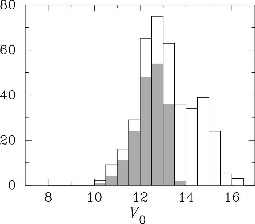
Figure 1: Distribution of the $V_{0}$ magnitude of our whole sample. The gray histogram presents the distribution of bright metal-poor star sample (see text)

In Table 1, we provide photometry and reddening data for our sample. The photometry data are taken from APASS for optical bands, and 2MASS (Skrutskie et al., 2006) for J and K. The reddening data are adopted from Green et al. (2018). The distribution of the $V_{0}$ magnitudes is shown in Figure 1. The gray histogram presents the $V_{0}$ distribution of the bright metal-poor star sample mentioned above (180 stars). The second peak of the distribution at $V_{0}\sim 15$ appears reflecting the sample selected to cover extremely metal-poor ranges.

3 High-resolution spectroscopy

3.1 Observations

High-resolution spectroscopy for selected candidates of very metal-poor stars has been obtained with the High Dispersion Spectrograph (HDS: Noguchi et al., 2002) of the Subaru Telescope. The spectra cover the wavelength region 4030–6800 Å with $R=36,000$ using the $2\times 2$ CCD binning.

The list of observing runs is given in Table 2. The observing runs were scheduled in units of half a night. The third column of the table gives the total number of nights for each run. The number of objects observed in each run is provided in the fourth column. There is duplication of objects that were observed in more than one observing runs.

We note that a portion of observing time of the intensive program was used for samples of other programs (e.g., stars in moving groups, Li-rich stars). One night of the August 2017 run was applied to observing candidates of extremely metal-poor stars with the HDS setup for the blue range.

3.2 Data reduction and data quality

Data reduction was carried out using the standard reduction procedure of the IRAF echelle package for HDS. It includes CCD bias level subtraction and linearity correction (Tajitsu et al., 2010), cosmic-ray removal following the procedure of Aoki et al. (2005), scattered-light subtraction and flat-fielding for 2D images. The spectra were extracted from the images and wavelengths were assigned using Th-Ar calibration spectra. The uncertainty of the wavelength calibration is less than 0.01 Å for our $R=36,000$ spectra. Sky background light was subtracted in the process of extraction when it is not negligible, i.e., more than a few percent of the peak count of the object. The observations have been conducted avoiding the targets close to the moon; however, the contamination of background light is significant in bright nights when the sky is covered by thin clouds. The process of sky subtraction in the data reduction was examined by visual inspection of the spectra for wide absorption features in the solar spectrum, e.g., the Mg I b lines at around 5180 Å, and the Fe I line at 4380 Å. A few spectra that are particularly affected by background light show unrealistically deep absorption lines in the blue regions, such as H$\gamma$ and H$\delta$ most likely due to over-subtraction of the sky spectrum. Such spectra are excluded from the sample for the abundance analysis in this work. The effect of sky is relatively severe in the data obtained in a night in 2016 May.

When there were multiple exposures for a star, the spectra obtained for individual exposures were combined for each object by summing up the individual exposures. The spectra extracted for individual echelle orders are combined by summing counts for overlapping wavelength ranges between adjacent orders. To obtain a normalized spectrum, a fit of the continuum level of spectra for individual echelle orders is made, and the derived profiles of the continuum are combined by summing counts as done for the original spectra. This provides a combined continuum spectrum. A normalized spectrum for the whole wavelength range is obtained by dividing the combined spectrum by the combined continuum spectrum. Examples of two portions of spectra are presented in Figures 2 and 3.

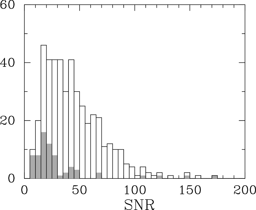
Figure 4: Distribution of the SNR (per pixel) of the whole sample in the program. The data not used for abundance analysis due to insufficient SNR or duplication of exposures are shown by the gray histogram. The object with the highest SNR is a double-lined spectroscopic binary (J 0241+0946), which is not included in the abundance study in Paper II.

The quality of the spectra varies considerably, because we set the minimum exposure time to 10 minutes, by which quite high SNR is achieved for the brightest targets, whereas only low SNR ($\sim 15$) is achieved by much longer exposures ($\sim$ 30 minute) for the faintest ones. The SNR is also dependent on the observing condition. Figure 4 shows the distribution of the SNR of data studied in this paper for radial velocity measurements. The SNR is estimated from the standard deviation of the data count in the wavelength range almost free from stellar spectral lines around 4500 Å. The value given in Table 3, and presented in the figure, is the SNR per pixel (1.8 km s^-1). The SNR per resolution element is approximately 2.2 times larger than that in the table and the figure. The SNR is also well approximated by the square root of the photon counts (Table 3), however, it is significantly lower in some objects that are affected by sky background.

The sample consists of 445 spectra of 420 stars including duplicated exposures. The radial velocities are investigated for the whole sample. The final sample of the chemical abundance measurements (385 stars) was determined through the abundance analysis process as the data quality is sufficiently high for the purpose taking account of the SNR and the number of Fe lines that can be used for abundance measurements, which depends on the effective temperature and metallicity (see Paper II for the details). The distribution of the SNR for the data not used for the abundance analysis is overplotted as a gray histogram in the figure.

4 Radial velocity measurements

Radial velocities of the program stars are determined through cross-correlation with the Subaru high-resolution spectrum for a VMP standard star, using the IRAF/fxcor. Fifteen orders in the wavelength range from 4230 through 5210 Å are used for each spectrum for the cross-correlation. The average value and the standard deviation of the 15 measured radial velocities are regarded as the adopted radial velocity and measurement uncertainty, respectively, for the corresponding spectrum. The typical uncertainty of the adopted radial velocity is about 0.14 km s^-1. Including the systematic errors due to instability of the instrument mostly due to temperature changes, the errors of radial velocity measurements from the Subaru spectra is $\lesssim 1$ km s^-1. The radial velocities measured from high-resolution spectra are given in Table 3.

Comparisons with radial velocities obtained from the LAMOST data release (DR5) are shown in Figure 5. No useful radial velocities are available from DR5 for several stars, some of which are most metal-poor objects. The sample is separated into two subsamples. One is a group of stars that show variations of radial velocities by more than 20 km s^-1 in the multi-epoch measurements with LAMOST. The criterion (20 km s^-1) is adopted taking account of the errors of the radial velocity measurements from LAMOST low-resolution spectra for our metal-poor stars (5-20 km s^-1) in DR5. The subsample consists of 56 stars. Variations of radial velocities suggest that the objects belong to binary systems with companions of faint main-sequence stars or white dwarfs, in the case of metal-poor stars around the main-sequence turn-off or the red giant branch. These stars are shown in the lower panel of Figure 5 with all the radial velocity data taken from LAMOST DR5. Significant variations of the radial velocities from LAMOST are found due to the above selection. Nevertheless, there is still a clear correlation between the values from LAMOST and Subaru. The mean and root-mean-square (r.m.s.) of the difference between radial velocities determined with Subaru and LAMOST ($V_{\rm Helio}$(Subaru) $-V_{\rm Helio}$(LAMOST)) are +3.6 and 14.0 km s^-1, respectively, excluding the data with differences larger than 40 km s^-1, i.e. twice the above criterion, which should be clearly affected by binary motions.

The other subsample includes stars with single-epoch LAMOST mearurements (201 stars), and those showing no significant variation of radial velocities ($<20$ km s^-1) in the LAMOST measurements (154 stars). The overall agreement between the radial velocities from LAMOST and Subaru is fairly good. The mean and r.m.s. of the difference between radial velocities determined with Subaru and LAMOST ($V_{\rm Helio}$(Subaru) $-V_{\rm Helio}$(LAMOST)) are +2.4 and 13.9 km s^-1, respectively, excluding the data with difference larger than 40 km s^-1. The difference of the radial velocities obtained by high-resolution spectroscopy from the LAMOST measurements is less than 20 km s^-1 for 158 objects among the 201 stars with single-epoch LAMOST observations. For 112 stars with multi-epoch LAMOST observations, the difference between the measurements of high-resolution spectroscopy and the average of the radial velocity of LAMOST measurements is less than 20 km s^-1. Hence, there is no signature of binarity for these 270 stars at this moment.

The radial velocities measured from high-resolution spectra of 85 stars differ from the measurements based on LAMOST spectra by more than 20 km s^-1. This set of stars consists of 43 stars with single-epoch and 42 with multiple-epoch LAMOST observations. These stars, as well as the 56 stars with large scatter of the radial velocities from the LAMOST measurements, are candidates of binary stars. Follow-up observations of these objects are desired to confirm their binarity and determine their orbital parameters. We note that five of the seven double-lined spectroscopic binaries discussed in § 6 are included in the sample of objects that show radial velocity variations.

In addition to the spectroscopic information, the astrometry from the Gaia mission can also be used to constrain the binarity of the objects. Gaia’s renormalized unit weight error (RUWE) is known to be sensitive to the presence of unresolved companions (Belokurov et al., 2020; Stassun & Torres, 2021). In our sample, there are 21 objects having RUWE$>1.4$. These objects are likely to have companions. Among them, seven stars show radial velocity variations, including J 0119-0121 and J 1435+1213, that show large variations among LAMOST measurements. For the remaining objects, no variation of radial velocity (larger than 20 km s^-1) is found. The frequency of stars that show radial velocity variations is 7/21 (33%), which is similar to the frequency in the whole sample (34%). The no excess of the frequency among the objects with large RUWE would at least be partially because the number of radial velocity measurements with LAMOST and Subaru is still quite limited. Another possible reason is that large RUWE could be found for objects with near face-on view, for which radial velocity variation is not detectable.

Figure 6 shows the distribution of heliocentric radial velocities of our sample. The distribution is well fit by a Gaussian with a central value of $V_{\rm Helio}=-29$ km s^-1. The offset of the central value is likely due to the selection bias of our sample that includes larger number of objects in the northern sky.

5 Interstellar absorption

We measured the equivalent widths of interstellar Na I D absorption lines when the interstellar component is separated from the stellar absorption. The measurements are made by direct integration of the interstellar absorption of D₁ and D₂ lines separately by IRAF/splot. The equivalent widths of both lines are measured for 324 objects.

We estimate the interstellar reddening, $E(B-V)$, adopting the relation between the reddening and the Na D line absorption given by Poznanski et al. (2012). We adopt the relation given by their equation (9) for the equivalent width $W$ combined for D₁ and D₂ lines. Their formula has a lower limit of $\log E(B-V)=-1.85$ ($E(B-V)=0.014$). For the weakest lines ($W<0.15$ Å) we assume a linear relation between $W$ and $E(B-V)$ as it connects to the above relation for larger $W$. Figure 7 shows a comparison of the $E(B-V)$ values obtained from the Na D line measurement with those derived from a dust map (Green et al., 2018). A fairly good correlation is found for most of the stars, whereas larger reddening is derived from the dust map for a dozen of stars. Some of the stars having larger $E(B-V)$ from the dust map than that from the interstellar absorption are nearby objects: This is found in the figure, where objects with a distance smaller than 0.5 kpc are presented by filled circles. For these objects the reddening might be overestimated from the dust map. On the other hand, there are several stars that have larger $E(B-V)$ from Na D lines than that from the dust map. We confirm by visual inspection of the spectra that the five objects with $E(B-V)$[Na D]$>0.1$ and $E(B-V)$[dust map]$<0.1$ exhibit strong interstellar absorption of Na D lines. The discrepancy of the $E(B-V)$ values for these stars might indicate scatter in the relation between the Na interstellar absorption and the dust extinction.

6 Double-lined spectroscopic binaries

Among the 420 stars for which high-resolution spectra are obtained, seven stars are identified as double-lined spectroscopic binaries that clearly exhibit pairs of absorption lines. Examples of spectral features are shown in Figure 8.

The radial velocity of each component is measured for Fe I lines that are isolated from other spectral features. Measurements are carried out by fitting Voigt profiles to two components separately using IRAF splot. The results are given in Table 4. The number of lines used in the analysis depends on the strengths of the absorption features and the data quality.

We also applied cross-correlation between the spectra of these stars and a template spectrum of a single star. Double peaks of the cross-correlation are found for stars with double lines that are clearly separated (e.g., J1220+1637, J1859+4506; see Figure 8), confirming the radial velocities determined from Fe I lines. We find that the second peak is not clear for stars that have only weak component of the secondary as expected. The radial velocities from Fe I lines are adopted as the final result.

Absorption features of the stronger component in the J 1216+0231 spectrum are slightly broader than those of the other component, as well as broader than the absorption features of the other stars. This might indicate that it is a triplet system, as SDSS J1108+1747 reported by Aoki et al. (2015). Further observations of this object at different phases will be needed to understand this system.

The velocity differences between the two components are 15 – 54 km s^-1. This range overlaps with that of the three double-lined spectroscopic binaries studied for the metal-poor stars found with SDSS and follow-up high-resolution spectroscopy (Aoki et al., 2015). The period and the binary separation of these systems would be smaller than 1000 days and several AU, respectively.

The $(V-K)_{0}$ color and absolute $V$ magnitude ($M_{V}$) of the objects are shown in Figure 9. The absolute magnitude is derived from the $V_{0}$ magnitude and the distance estimated by the parallax of Gaia DR2 (Gaia Collaboration et al., 2016, 2018). Isochrones of the Yonsei-Yale stellar evolution models (Kim et al., 2002) are shown for the metallicity range $-3.5\leq$[Fe/H]$\leq-1.5$. The double-lined spectroscopic binaries found by our study are located in the main-sequence turn-off range. This is expected because the luminosity is very sensitive to mass in red giants and, hence, the primary is dominant in the system if it has already evolved to a red giant.

We here estimate the contribution of each component of the binary system to the overall flux from the strengths of the absorption lines. The depth of the absorption lines of Mg I b lines around 5180 Å is not very sensitive to the effective temperature in the range of the main-sequence turn-off ($5500$ K$<$$T_{\mbox{\scriptsize eff}}$$<6500$  K). Hence, we assume that the apparent depths of the Mg lines are approximately proportional to the contributions of the two components to the flux in the $V$ band. The open circles in Figure 9 indicate the absolute magnitudes of the primaries. Here the color of the primary is assumed to be the same as that of the system. This is a good approximation for systems in which the primary is dominant, or when the two components have similar luminosity and $T_{\mbox{\scriptsize eff}}$. The most uncertain case is a system that includes a subgiant, since the luminosity (absolute magnitude) is similar in a relatively wide ranges of $T_{\mbox{\scriptsize eff}}$ and $V-K$ color. The 10% uncertainty in the estimate of the contribution of a component to the luminosity results in about $\pm 250$ K uncertainty of $T_{\mbox{\scriptsize eff}}$ according to the isochrone.

Figure 9 clearly indicates that the primary stars are on the main-sequence in most cases. The secondary should also be on the main-sequence, having larger $(V-K)_{0}$ color, with similar or larger (fainter) absolute magnitude, than the primary. An exception is J 1216+0231 ($M_{V}=2.7$) whose primary star would be on the subgiant branch. This system could be triplet as mentioned above. To understand the system, further monitoring of the variations of spectral features is desirable.

We estimate the metallicity of the primary stars adopting the equivalent widths of the Fe lines used to measure the radial velocities. The equivalent widths are corrected by the contribution of the primary star to the flux estimated above (Table 5). The effective temperature is estimated from colors as done for our whole sample that will be reported in Paper II. The surface gravity and microturbulent velocity are fixed to $\log g=4.0$ and $v_{\rm t}=1.5$ km s^-1, respectively, which are sufficient for the present purpose. The metallicity ([Fe/H]) of our sample ranges from $-1.8$ to $-3.2$, confirming that they are very metal-poor, although the uncertainty of the [Fe/H] values is as large as 0.5 dex, primarily due to the uncertainties in the estimate of the contribution of the primary star to the flux.

The above analysis indicates that the seven objects are all binary systems of very metal-poor stars with short periods ($<1000$ days), as the three objects studied by Aoki et al. (2015) from the SDSS sample. The number of main-sequence turn-off stars ($T_{\rm eff}>$ 5500 K) in our whole sample is 242. The fraction of double-lined spectroscopic binaries detected by single-epoch observations, 7/242= 2.9%, is similar to that obtained by Aoki et al. (2015): 3/109=2.8%. We note that the distribution of effective temperature in $T_{\rm eff}>$ 5500 K of the whole sample is also similar to that of Aoki et al. (2015). Aoki et al. (2015) discussed the frequency of binary systems with short periods at very low metallicity is at least 10 %, taking the detection probability of the systems by a single epoch observation into account. The result of the present study supports this argument by increasing the sample size.

The frequency of binaries has been studied by a variety of spectroscopic survey projects. Moe et al. (2019) recently investigated the metallicity dependence of binary frequency by compiling previous studies including the Carney-Lathum sample (e.g., Carney et al., 2005; Latham et al., 2002), Rastegaev (2010), SDSS and LAMOST (Hettinger et al., 2015; Gao et al., 2017), SDSS/APOGEE (Badenes et al., 2018), and very metal-poor stars (Hansen et al., 2015). Applying corrections for completeness of the survey depending on metallicity, i.e. lower completeness for metal-poor stars due to weakness of absorption lines, they conclude that the fraction of close binaries ($P<10,000$ days) is higher at lower metallicity, reaching about 50% at [Fe/H]$=-3$. It should be noted that the original sample of very metal-poor stars referred to in their work is still small: 91 stars with [Fe/H]$<-0.9$ were studied by Carney et al. (2005) and 41 r-process-enhanced stars with [Fe/H]$<-1.6$ were studied by Hansen et al. (2015). Although the frequency of binaries directly estimated for these samples is 15-20%, the correction estimated by Moe et al. (2019) is as large as a factor of three at the lowest metallicity. The frequency of double-lined spectroscopic binaries with $P<1000$ days estimated by our study is well below the frequency of all binary systems that include pairs of stars having significantly different luminosity.

At higher metallicity ([Fe/H]$>-1$), a much larger number of double-lined spectroscopic binaries has been identified by high-resolution spectroscopic surveys. El-Badry et al. (2018) reported the detection of about 2500 binaries from 20,000 main-sequence stars of the APOGEE sample. More recently, Traven et al. (2020) studied more than 580,000 stars of the GALAH survey sample (including red giants), identifying 12,760 double-lined spectroscopic binaries. Most of them are main-sequence stars as expected. The fraction of double-lined spectroscopic binaries in their sample, about 2%, should be significantly higher if the sample is limited to main-sequence. However, the frequency estimated by the present work for VMP/EMP stars, about 10%, seems to be higher than that found for metal-rich stars, supporting theoretical studies of binary formation at very low metallicity (e.g., Machida, 2008).

7 Summary

We acquired high-resolution spectroscopy using the Subaru Telescope High Dispersion Spectrograph for about 400 very metal-poor stars selected by means of LAMOST low-resolution spectroscopy. This paper reports on the observing program, including sample selection, observations and data reduction, estimates of extinction from interstellar Na I D lines, and radial velocities. Based on the detection of seven double-lined spectroscopic binaries, the frequency of binary systems with short periods is discussed. The data are used for detailed abundance analyses that are reported separately in paper II of this series.

.

Figure 2: Examples of spectra of a metal-poor giant, an extremely metal-poor giant, a metal-poor turn-off star, and an extremely metal-poor turn-off star from top to bottom. The name of object is presented in each panel.

Figure 3: The same as Figure 2, but for a different wavelength range.

Figure 5: Comparison of the heliocentric radial velocities obtained from the Subaru high-resolution spectra with LAMOST measurements. Upper panel: Objects for which no variation of radial velocity is detected by LAMOST measurements, including those with single-epoch LAMOST observation. Lower panel: Objects for which radial velocity variation ($>20$ km s^-1) is detected in the LAMOST measurements. The solid lines indicate one-to-one relationship, and the dotted lines are those shifted by 20 km s^-1.

Figure 6: Distribution of the heliocentric radial velocities of our sample.

Figure 7: Reddening obtained from the Na D₁ and D₂ line absorption compared with that from the dust map. Filled circles are objects with distances smaller than 0.5 kpc.

Figure 8: Spectra of double-lined spectroscopic binaries. The names of the objects are presented in the panel.

Figure 9: Color-Magnitude diagam for the double-lined spectroscopic binaries. The $(V-K)_{0}$ and $M_{V}$ for the objects are shown by filled circles. The open circles indicate the $M_{V}$ values estimated for the primary stars in the systems (see text). The lines show the isochrones of Yonsei-Yale models (Kim et al., 2002) with enhancement of $\alpha$ elements for 12 Gyr for [Fe/H]$=-1.5$ (solid), $-2.0$ (dashed), $-2.5$ (dot-dashed), $-3.5$ (dotted).

Table 1: Objects studied with high-resolution spectra

Short ID	Object name	$V$	$E(B-V)$		$B_{0}$	$V_{0}$	$g_{0}$	$r_{0}$	$J_{0}$	$K_{0}$
			dust map	Na D
J0002+0343	LAMOST J000235.04+034337.5	15.094	0.028	0.024	15.446	15.019	15.068	14.894	14.062	13.738
J0003+1556	LAMOST J000310.89+155601.8	12.321	0.058	0.035	12.747	12.166	12.368	11.912	10.779	10.312
J0006+0123	LAMOST J000637.82+012343.3	13.123	0.036	0.041	13.793	13.028	13.487	13.008	11.856	11.470
J0006+1057	LAMOST J000617.20+105741.8	12.912	0.070	0.043	13.555	12.725	13.076	12.590	10.954	10.330
J0013+2350	LAMOST J001351.30+235049.1	12.328	0.053	0.041	12.608	12.187	12.305	12.053	11.173	10.876

Table 2: Observing Runs

Proposal ID	Obs. dates	number of nights	number of objects
S14A-112	May 9-10, 2014	2	51
S15A-093	March 5, 2015	1	10
S15B-087	November 28-29, 2015	2	42
S16A-119I	April 26-27, 2016	1	18
S16A-119I	May 20, 22, 23, 27, 28, 2016	5	123
S16A-119I	November 16-19, 2016	4a	49
S16A-119I	February 15-19, 2017	5	84
S16A-119I	August 1-5, 2017	2.5a,b	27
S16A-119I	January 24-27, 2018	2.5c	0

Table 3: Observation and kinematics information

Short ID	date of observation	SNR	$V_{\rm Helio}$	$\sigma(V_{\rm Helio})$	Parallax	error	Distance	error
			(km s-1)	(km s-1)	(mas)	(mas)	(pc)	(pc)
J0002+0343	20151129	23.7	$-91.4$	0.8	0.647	0.050	1465	109
J0003+1556	20161116	32.2	$-185.5$	0.1	0.3623	0.0542	2380	298
J0006+0123	20161119	44.1	$-65.9$	0.2	0.6591	0.0368	1446	78
J0006+1057	20161116	21.9	$-312.4$	0.3	0.1103	0.0425	4549	686
J0013+2350	2017 8 4	41.4	$-259.2$	0.1	2.0484	0.0384	482	9

Table 4: Double-lined spectroscopic binaries

Object	$V_{\rm Helio,A}$	error	$V_{\rm Helio,B}$	error	$N$	[Fe/H]
	(km s-1)	(km s-1)	(km s-1)	(km s-1)
J0241$+$0946	$-72.32$	0.04	$-57.25$	0.05	45	$-2.1$
J1144$+$4032	$-15.22$	0.04	$13.81$	0.23	26	$-2.2$
J1216$+$0231	$52.473$	1.25	$106.41$	0.69	7	$-2.9:$
J1220$+$1637	$-83.192$	0.28	$-38.73$	0.33	7	$-3.2$
J1231$+$1232	$32.17$	0.09	$14.67$	0.16	38	$-2.3$
J1859$+$4506	$-292.42$	0.19	$-251.61$	0.19	14	$-2.9$
J2121$-$0138	$13.55$	0.07	$32.72$	0.08	41	$-1.8$

Table 5: Equivalent widths of Fe I lines in the primary stars of double-lined spectroscopic binaries

Wavelength	$\log gf$	L.E.P.	J0241$+$0946	1144$+$4032	J1216$+$0231	J1220$+$1637	J1231$+$1232	J1859$+$4506	J2121$-$0138
(Å)		(eV)	(mÅ)	(mÅ)	(mÅ)	(mÅ)	(mÅ)	(mÅ)	(mÅ)
4063.594	0.062	1.558	157.6	$\cdots$	81.2	$\cdots$	107.8	111.6	170.6
4071.738	$-$0.008	1.608	119.6	$\cdots$	83.8	71.2	110.5	80.1	139.9
4132.058	$-$0.675	1.608	99.8	110.0	40.8	$\cdots$	71.6	$\cdots$	106.1
4181.755	$-$0.370	2.832	54.4	$\cdots$	$\cdots$	$\cdots$	$\cdots$	21.6	60.9
4187.795	$-$0.554	2.425	63.6	$\cdots$	$\cdots$	$\cdots$	$\cdots$	$\cdots$	67.5
4191.430	$-$0.670	2.469	46.0	$\cdots$	$\cdots$	$\cdots$	65.7	$\cdots$	64.8

References

- Aoki et al. (2018) Aoki, W., Matsuno, T., Honda, S., et al. 2018, PASJ, 70, 94, doi: 10.1093/pasj/psy092
- Aoki et al. (2017) —. 2017, PASJ, 69, 21, doi: 10.1093/pasj/psw125
- Aoki et al. (2015) Aoki, W., Suda, T., Beers, T. C., & Honda, S. 2015, AJ, 149, 39, doi: 10.1088/0004-6256/149/2/39
- Aoki et al. (2014) Aoki, W., Tominaga, N., Beers, T. C., Honda, S., & Lee, Y. S. 2014, Science, 345, 912, doi: 10.1126/science.1252633
- Aoki et al. (2005) Aoki, W., Honda, S., Beers, T. C., et al. 2005, ApJ, 632, 611, doi: 10.1086/432862
- Aoki et al. (2013) Aoki, W., Beers, T. C., Lee, Y. S., et al. 2013, AJ, 145, 13, doi: 10.1088/0004-6256/145/1/13
- Badenes et al. (2018) Badenes, C., Mazzola, C., Thompson, T. A., et al. 2018, ApJ, 854, 147, doi: 10.3847/1538-4357/aaa765
- Barklem et al. (2005) Barklem, P. S., Christlieb, N., Beers, T. C., et al. 2005, A&A, 439, 129, doi: 10.1051/0004-6361:20052967
- Belokurov et al. (2020) Belokurov, V., Penoyre, Z., Oh, S., et al. 2020, MNRAS, 496, 1922, doi: 10.1093/mnras/staa1522
- Bonifacio et al. (2015) Bonifacio, P., Caffau, E., Spite, M., et al. 2015, A&A, 579, A28, doi: 10.1051/0004-6361/201425266
- Carney et al. (2005) Carney, B. W., Aguilar, L. A., Latham, D. W., & Laird, J. B. 2005, AJ, 129, 1886, doi: 10.1086/427542
- Castelli & Kurucz (2003) Castelli, F., & Kurucz, R. L. 2003, in IAU Symposium, Vol. 210, Modelling of Stellar Atmospheres, ed. N. Piskunov, W. W. Weiss, & D. F. Gray, 20P–+
- Cayrel et al. (2004) Cayrel, R., Depagne, E., Spite, M., et al. 2004, A&A, 416, 1117, doi: 10.1051/0004-6361:20034074
- Christlieb et al. (2008) Christlieb, N., Schörck, T., Frebel, A., et al. 2008, A&A, 484, 721, doi: 10.1051/0004-6361:20078748
- Cohen et al. (2013) Cohen, J. G., Christlieb, N., Thompson, I., et al. 2013, ApJ, 778, 56, doi: 10.1088/0004-637X/778/1/56
- Cohen et al. (2004) Cohen, J. G., Christlieb, N., McWilliam, A., et al. 2004, ApJ, 612, 1107, doi: 10.1086/422576
- De Silva et al. (2015) De Silva, G. M., Freeman, K. C., Bland-Hawthorn, J., et al. 2015, MNRAS, 449, 2604, doi: 10.1093/mnras/stv327
- El-Badry et al. (2018) El-Badry, K., Ting, Y.-S., Rix, H.-W., et al. 2018, MNRAS, 476, 528, doi: 10.1093/mnras/sty240
- Frebel & Norris (2015) Frebel, A., & Norris, J. E. 2015, ARA&A, 53, 631, doi: 10.1146/annurev-astro-082214-122423
- Freeman & Bland-Hawthorn (2002) Freeman, K., & Bland-Hawthorn, J. 2002, ARA&A, 40, 487, doi: 10.1146/annurev.astro.40.060401.093840
- Gaia Collaboration et al. (2016) Gaia Collaboration, Prusti, T., de Bruijne, J. H. J., et al. 2016, A&A, 595, A1, doi: 10.1051/0004-6361/201629272
- Gaia Collaboration et al. (2018) Gaia Collaboration, Brown, A. G. A., Vallenari, A., et al. 2018, A&A, 616, A1, doi: 10.1051/0004-6361/201833051
- Gao et al. (2017) Gao, S., Zhao, H., Yang, H., & Gao, R. 2017, MNRAS, 469, L68, doi: 10.1093/mnrasl/slx048
- Gilmore et al. (2012) Gilmore, G., Randich, S., Asplund, M., et al. 2012, The Messenger, 147, 25
- Green et al. (2018) Green, G. M., Schlafly, E. F., Finkbeiner, D., et al. 2018, MNRAS, 478, 651, doi: 10.1093/mnras/sty1008
- Hansen et al. (2015) Hansen, T. T., Andersen, J., Nordström, B., et al. 2015, A&A, 583, A49, doi: 10.1051/0004-6361/201526812
- Heger & Woosley (2010) Heger, A., & Woosley, S. E. 2010, ApJ, 724, 341, doi: 10.1088/0004-637X/724/1/341
- Hettinger et al. (2015) Hettinger, T., Badenes, C., Strader, J., Bickerton, S. J., & Beers, T. C. 2015, ApJ, 806, L2, doi: 10.1088/2041-8205/806/1/L2
- Honda et al. (2004) Honda, S., Aoki, W., Kajino, T., et al. 2004, ApJ, 607, 474, doi: 10.1086/383406
- Jacobson et al. (2015) Jacobson, H. R., Keller, S., Frebel, A., et al. 2015, ApJ, 807, 171, doi: 10.1088/0004-637X/807/2/171
- Keller et al. (2014) Keller, S. C., Bessell, M. S., Frebel, A., et al. 2014, Nature, 506, 463, doi: 10.1038/nature12990
- Kim et al. (2002) Kim, Y.-C., Demarque, P., Yi, S. K., & Alexander, D. R. 2002, ApJS, 143, 499, doi: 10.1086/343041
- Lai et al. (2008) Lai, D. K., Bolte, M., Johnson, J. A., et al. 2008, ApJ, 681, 1524, doi: 10.1086/588811
- Latham et al. (2002) Latham, D. W., Stefanik, R. P., Torres, G., et al. 2002, AJ, 124, 1144, doi: 10.1086/341384
- Li et al. (2015a) Li, H., Aoki, W., Zhao, G., et al. 2015a, PASJ, 67, 84, doi: 10.1093/pasj/psv053
- Li et al. (2018) Li, H., Tan, K., & Zhao, G. 2018, ApJS, 238, 16, doi: 10.3847/1538-4365/aada4a
- Li et al. (2015b) Li, H.-N., Aoki, W., Honda, S., et al. 2015b, Research in Astronomy and Astrophysics, 15, 1264, doi: 10.1088/1674-4527/15/8/011
- Liang et al. (2018) Liang, X. L., Zhao, J. K., Zhao, G., et al. 2018, ApJ, 863, 4, doi: 10.3847/1538-4357/aacf8a
- Machida (2008) Machida, M. N. 2008, ApJ, 682, L1, doi: 10.1086/590109
- Majewski et al. (2017) Majewski, S. R., Schiavon, R. P., Frinchaboy, P. M., et al. 2017, AJ, 154, 94, doi: 10.3847/1538-3881/aa784d
- Moe et al. (2019) Moe, M., Kratter, K. M., & Badenes, C. 2019, ApJ, 875, 61, doi: 10.3847/1538-4357/ab0d88
- Noguchi et al. (2002) Noguchi, K., Aoki, W., Kawanomoto, S., et al. 2002, PASJ, 54, 855, doi: 10.1093/pasj/54.6.855
- Nomoto et al. (2013) Nomoto, K., Kobayashi, C., & Tominaga, N. 2013, ARA&A, 51, 457, doi: 10.1146/annurev-astro-082812-140956
- Nordlander et al. (2019) Nordlander, T., Bessell, M. S., Da Costa, G. S., et al. 2019, MNRAS, 488, L109, doi: 10.1093/mnrasl/slz109
- Poznanski et al. (2012) Poznanski, D., Prochaska, J. X., & Bloom, J. S. 2012, MNRAS, 426, 1465, doi: 10.1111/j.1365-2966.2012.21796.x
- Rastegaev (2010) Rastegaev, D. A. 2010, AJ, 140, 2013, doi: 10.1088/0004-6256/140/6/2013
- Skrutskie et al. (2006) Skrutskie, M. F., Cutri, R. M., Stiening, R., et al. 2006, AJ, 131, 1163, doi: 10.1086/498708
- Stassun & Torres (2021) Stassun, K. G., & Torres, G. 2021, ApJ, 907, L33, doi: 10.3847/2041-8213/abdaad
- Tajitsu et al. (2010) Tajitsu, A., Aoki, W., Kawanomoto, S., & Narita, N. 2010, Publications of the National Astronomical Observatory of Japan, 13, 1
- Traven et al. (2020) Traven, G., Feltzing, S., Merle, T., et al. 2020, A&A, 638, A145, doi: 10.1051/0004-6361/202037484
- Venn et al. (2020) Venn, K. A., Kielty, C. L., Sestito, F., et al. 2020, MNRAS, 492, 3241, doi: 10.1093/mnras/stz3546
- Xing et al. (2019) Xing, Q.-F., Zhao, G., Aoki, W., et al. 2019, Nature Astronomy, 3, 631, doi: 10.1038/s41550-019-0764-5
- Yan et al. (2022) Yan, H.-L., Li, H., Wang, S., et al. 2022, The Innovation, in press, doi: 10.1016/j.xinn.2022.100224
- Yan et al. (2021) Yan, H.-L., Zhou, Y.-T., Zhang, X., et al. 2021, Nature Astronomy, 5, 86, doi: 10.1038/s41550-020-01217-8
- Yanny et al. (2009) Yanny, B., Rockosi, C., Newberg, H. J., et al. 2009, AJ, 137, 4377, doi: 10.1088/0004-6256/137/5/4377
- Yong et al. (2013) Yong, D., Norris, J. E., Bessell, M. S., et al. 2013, ApJ, 762, 26, doi: 10.1088/0004-637X/762/1/26
- Yong et al. (2021) Yong, D., Da Costa, G. S., Bessell, M. S., et al. 2021, arXiv e-prints, arXiv:2107.06430. https://arxiv.org/abs/2107.06430
- Zhang et al. (2019) Zhang, S., Li, H., Zhao, G., Aoki, W., & Matsuno, T. 2019, PASJ, 71, 89, doi: 10.1093/pasj/psz071
- Zhao et al. (2012) Zhao, G., Zhao, Y.-H., Chu, Y.-Q., Jing, Y.-P., & Deng, L.-C. 2012, Research in Astronomy and Astrophysics, 12, 723, doi: 10.1088/1674-4527/12/7/002
- Zhao et al. (2018) Zhao, J. K., Zhao, G., Aoki, W., et al. 2018, ApJ, 868, 105, doi: 10.3847/1538-4357/aae712