Repulsive gravity effects in horizon formation

Abstract

Repulsive gravity is a well known characteristic of naked singularities. In this work, we explore light surfaces and find new effects of repulsive gravity. We compare Kerr naked singularities with the corresponding black hole counterparts and find certain structures that are identified as horizon remnants. We argue that these features might be significant for the comprehension of processes that lead to the formation or eventually destruction of black hole Killing horizons. These features can be detected by observing photon orbits, particularly close to the rotation axis, which can be used to distinguish naked singularities from black holes.

1 Introduction

We explore possible effects of repulsive gravity in the formation of horizons by studying structures appearing in the light surfaces of a class of very slowing spinning Kerr naked singularities (NSs), variously studied in literature in connection with the Killing horizon properties of the Kerr black holes (BHs) bundle-EPJC-complete ; observers ; remnants ; Pugliese:2019efv ; Pugliese:2019rfz ; LQG-bundles ; PS . Negative gravity effects appear related with a peculiar feature of light surfaces that can be detected by observing photon orbits. We investigate photon circular orbits with orbital frequencies (relativistic velocities) equal in magnitude to the BH horizon frequencies.

The frequency of photon orbits relate NSs to BHs. We shall see that there is a correspondence with singularities having spin mass ratio $M/a$ and $a/M$, known as BH-NS dualism–see alsoMankoaERuizb ). From the observational view point the detection of these photons, especially close to the poles ($\theta\approx 0$) can provide information on the property of the horizons or eventually can detect a non horizon existence distinguishing NSs from BHs, constituting an observational target for example for the Event Horizon Telescope ETH1 . Light surfaces delimiting stationary observer frequencies in NS spacetimes bound a region, Killing throat, appearing as the “opening” and disappearance of the Killing horizons of the corresponding BH geometries. A Killing bottleneck is a particular structure of Killing throat appearing as throat “restrictions" only in slowly spinning NSs. Killing bottlenecks appear in association with the concept of pre-horizon regime introduced in de-Felice1-frirdtforstati ; de-Felice-first-Kerr . For this reason, Killing bottleneck are also called horizon remnants. There is a pre-horizon regime in the spacetime when there are mechanical effects allowing circular orbit observers to recognize the close presence of an event horizon. For instance, a gyroscope would observe a “memory” of the static or stationary initial state in the Kerr metric. The relevance of this feature during the gravitational collapse is discussed in de-Felice3 ; de-Felice-mass ; de-Felice4-overspinning ; Chakraborty:2016mhx . Similar structures were also studied in Tanatarov:2016mcs and Mukherjee:2018cbu ; Zaslavskii:2018kix ; Zaslavskii:2019pdc . It has been argued that these structures could play an important role in the description of BH formation and for testing the possible existence of NSs de-Felice3 ; de-Felice-mass ; de-Felice4-overspinning ; Chakraborty:2016mhx .

Here we study Killing bottlenecks, providing their characteristic frequencies and orbital regions where they can be observed. We frame them in relation to the effects of repulsive gravity and provide a description of the corresponding photon orbits. Bottleneck structures find an explanation in the context of metric bundles (MBs), which are particular curves grouping different Kerr geometries that allow us to reinterpret the concept of horizon and to connect BHs and NSs through the photon frequency $\omega$. The bottleneck is also a characteristic of the ergoregion.

The effects of repulsive gravity in the case of the Kerr geometry were considered in 1975A&A….45…65D ; MankoaERuizb ; QM ; LQ ; Patil:2011aw ; Maluf:2014nsa . Typical effects of repulsive gravity were observed in the naked singularity ergoregion, with zero and negative energy states in circular orbits Stu80 ; Gariel:2014ara ; Pelavas:2000za ; Herdeiro:2014jaa ; Stuchlik:2014jua . On the other hand, the presence of negative energy particles is a distinctive feature of the ergoregion of any spinning source. Eventually this special matter, constituting an “antigravity” sphere, can possibly be filled with negative energy formed according to the Penrose process, and bounded by orbits with zero angular momentum (ZAMOS). It has been argued that the ergoregion cannot disappear as a consequence of a change in spin, because it may be filled by negative energy matter– Chakraborty:2016mhx ; Frolov:2014dta see also Negative . Quantum evaporation of NSs was analyzed in Goswami:2005fu , radiation in Vaz:1998gd , and gravitational radiation in Iguchi:1999ud ; Iguchi:1998qn ; Iguchi:1999jn Concerning the ergoregion stability, see for example, Cardoso:2007az ; CoSch .)

Finally, we note that under general initial data on the progenitors, the gravitational collapse analysis does not rule out the possibility that NSs can be produced as the result of a gravitational collapse miller ; Penrose ; Shapiro ; Santos ; Avi2020 ; Joshi ; Harada ; 1999JApA…20..233P ; Joshi:2001xi ; Shapiro-Shapiro ; Berger ; Bousso . The process of gravitational collapse is constrained by the Penrose cosmic censorship to “good" initial conditions to end up with horizons formation; on the other hand, the problem of gravitational collapse involves many factors including symmetries during the collapse. Consequently, the issue of NS consistency (BH formation) is still openSantos ; Avi2020 ; Joshi ; Harada . Remaining a conjecture, the results depend on the physical initial conditions. (For stars or galaxy BH progenitors, with spin $a=J/(Mc)$, usually larger than the mass $m=GM/c^{2}$, it is supposed to lose mass and angular momentum during the gravitational collapse towards the singularity.) The issue of NS (BH) creation is parallelized with the issue of NS stability–see for example Sha-teu91 ; ApTho ; J-S09 ; Jacobson:2010iu ; Esitenza ; Giacomazzo:2011cv .

This work is organized as follows. Sec. (2) introduces the Kerr geometry and Kerr horizons. Bottlenecks are represented by curves in the metric bundles and recognized by observing particular photon circular orbits, horizon replicas, which are defined in Sec. (2.1). Sec. (3) contains a formal definition of bottlenecks, expressed in terms of the metric bundles and horizon angular momentum (or photon impact parameter). Then, bottlenecks are studied on the equatorial plane. A description of the peculiar effects of repulsive gravity on circular motion in the region of the bottleneck is also provided. As evidenced by the metric bundles analysis, the bottlenecks are characterized by the closeness of the photon orbital frequency values delimiting also the orbits accessible to the stationary observers (this range is null on the BHs horizons). Each frequency is demonstrated to correspond to a BH horizon frequency. Bottlenecks can be observed on horizons replicas, which we discuss in Sec. (3.1), considering also the counter-rotating orbits, replicating the frequencies of the inner and outer BH horizons.

2 Kerr geometry and Killing horizons

The line element of the Kerr geometry can be written as

$$\differential s^{2}=-\alpha^{2}\differential t^{2}+\frac{A\sigma}{\rho^{2}}(\differential\phi-\omega_{z}\differential t)^{2}+\frac{\rho^{2}}{\Delta}\differential r^{2}+\rho^{2}\differential\theta^{2},$$ (1)

$$\sigma\equiv\sin^{2}\theta,\quad A\equiv(r^{2}+a^{2})^{2}-a^{2}\Delta\sigma$$ (2)

$$\Delta\equiv r^{2}-2Mr+a^{2},\quad\mbox{and}\quad\rho^{2}\equiv r^{2}+a^{2}(1-\sigma),$$ (3)

in Boyer-Lindquist coordinates. $M\geq 0$ is interpreted as the mass of the gravitational source and $a\equiv J/M$ is the specific angular momentum (spin), while $J$ is the total angular momentum. A naked singularity occurs for $a>M$. In Eq. (1), $\alpha=\sqrt{\Delta\rho^{2}/A}$ and $\omega_{z}=2aMr/A$ are, respectively, the lapse function and the frequency of the zero angular momentum fiducial observer (ZAMO), whose four-velocity is $u^{a}=(1/\alpha,0,0,\omega_{z}/\alpha)$ orthogonal to the surface of constant $t$ observers . In the following, to simplify the discussion, when not otherwise specified, we use geometrical units with $r\rightarrow r/M$ and $a\rightarrow a/M$.

Killing horizons

The inner and outer Killing horizons and the inner and outer ergosurfaces for the Kerr geometry are located at

$$r_{\mp}=M\mp\sqrt{M^{2}-a^{2}},\quad r_{\epsilon}^{\mp}=M\mp\sqrt{M^{2}-a^{2}\cos^{2}\theta},$$ (4)

respectively. The outer ergosurface, $r_{\epsilon}^{+}$ is a time-like surface defined by the vanishing of the norm of the Killing vector representing time translations at infinity, $\partial_{t}$. Killing horizons are the light-like hypersurface, generated by the flow of a Killing vector, on which the norm of the Killing vector vanishes, that is, the null generators coincide with the orbits of an one-parameter group of isometries: there exists a Killing field $\mathcal{L}$, which is normal to $\mathcal{S}_{0}$. The event horizons of the Kerr BH are Killing horizons with respect to the Killing field $\mathcal{L}_{H}=\partial_{t}+\omega_{H}^{\pm}\partial_{\phi}$, where $\omega_{H}^{\pm}$ is the angular velocity (frequency) of the horizons, respectively. (The vectors $\xi_{t}=\partial_{t}$ and $\xi_{\phi}=\partial_{\phi}$ are, respectively, the stationary and axisymmetric Killing fields. In the limiting case of spherically symmetric, static spacetimes, the event horizons are Killing horizons with respect to the Killing vector $\partial_{t}$ and the event, apparent, and Killing horizons with respect to the Killing field $\xi_{t}$ coincide.) The results we discuss in this work follow from the investigation of the properties of the Killing vector $\mathcal{L}=\partial_{t}+\omega\partial_{\phi}$, for photon-like particles with rotational frequencies $\omega=\omega_{\pm}:\mathcal{L}\cdot\mathcal{L}=0$. This vector $\mathcal{L}$ is related also to the definition of stationary observes with four-velocity bounded by the limiting relativistic photon velocities $\omega_{\pm}$. On the BH horizons, $r_{\pm}$, there is $\omega_{\pm}(r_{\pm})=\omega_{H}^{\pm}$. The relation $\mathbf{\mathcal{L_{N}}}\equiv\mathcal{L}\cdot\mathcal{L}=0$ defines the light-surfaces we consider here. The “rotation term” $\omega_{H}^{+}$ plays an important role in BH thermodynamics. Indeed, in the first first law of BH thermodynamics, for a variation of the total mass $\delta M$, the term $\omega^{+}_{H}(0)\delta J$ can be interpreted as the “work term”, where $(0)$ refers to the state prior to the transition)–e.g. Wald:1999xu ; WWW ; inprogress . The Kerr BH surface gravity can be written as the combination $\kappa=\kappa_{s}-\gamma_{a}$, where $\kappa_{s}\equiv{{1}/{4M}}$ is the Schwarzschild surface gravity, while $\gamma_{a}=M(\omega_{H}^{+})^{2}$ is the contribution due to the additional component of the BH intrinsic spin. Therefore, $\omega_{H}^{+}$ is the angular velocity, in units of $1/M$, on the event horizon. In the extreme BH case, the surface gravity is zero and the temperature $T_{H}=0$, with consequences also with respect to the stability against Hawking radiation. However, the entropy (or BH area) of an extremal BH is not null. An implication of the third law of BH thermodynamics is that there is no physical process reaching from a non-extremal BH an extremal BH in a finite number of steps Chrusciel:2012jk ; Wald:1999xu ; Li:2013sea ; Jacobson:2010iu ; Sha-teu91 ; Goswami:2005fu . The surface area of the BH event horizon is non-decreasing in time, which is the content of the second law. The thermodynamic laws state also the impossibility to reach by a physical process a BH state with surface gravity $\kappa=0$.

2.1 Metric bundles and horizons replicas

In NSs, the frequencies $\omega_{\pm}$ are also BH horizon frequencies establishing a BH-NS connection. The proximity of the frequencies $\omega$ in NSs, with the values of the BH horizons frequencies can be described by metric bundles (MBs), introduced in observers ; remnants ; Pugliese:2019efv ; Pugliese:2019rfz ; LQG-bundles ; PS ; bundle-EPJC-complete .

Kerr metric bundles: A Kerr metric bundle is defined as the solution of $a:\mathcal{L}_{\mathcal{N}}(\bar{\omega})=0$, for a fixed constant $\bar{\omega}$, (bundle characteristic frequency). It collects all and only Kerr geometries with a (circular) photon orbit (replica) having the same orbital frequency $\bar{\omega}$, which is the value of the limiting frequencies $\omega_{\pm}$. A bundle can be represented by a curve in the plane $r/M-\mathcal{A}/M$ (extended plane), where $\mathcal{A}\equiv a\sqrt{\sigma}$; on the equator the plane is $r-a$. In this plane, the curve, $a_{\pm}\equiv\sqrt{r(2M-r)}$, represents the horizons of all the Kerr BHs. Each point of the curve is an inner, for $r\in]0,M]$ (with $\omega>1/2$), or outer, for $r\in[M,2M]$ (with $\omega\in]0,1/2[$), Killing horizon of a Kerr BH–Figs (1). The bundle origin, for $r=0$, is the spin $a_{0}\equiv 1/\omega\sqrt{\sigma}$ (alternatively $\mathcal{A}_{0}\equiv 1/\omega$). All the bundle curves are tangent to the horizon curve $a_{\pm}$ and the horizon curve is the envelope surface of all the MB curves. Therefore, the bundle characteristic frequency $\omega$ is also the BH horizon frequency ($\omega_{H}^{+}$ or $\omega_{H}^{-}$), defined by the tangent point of the bundle curve to the horizon curve. MBs are represented in Figs (1). MBs can contain either only BH geometries or NS and BH geometries.

Horizon replicas and horizon confinement: Replicas connect structures in different spacetimes characterized by equal value of the property $\mathcal{Q}$. Let $\mathcal{Q}({r_{p}})$ be a quantity characteristic of the horizon $r_{p}$ (for the BH spacetime with spin $a_{p}$) in the extended plane. There is a horizon replica in a spacetime $a_{q}$, if there exists a radius (orbit) $r_{q}$ such that $\mathcal{Q}(r_{q},a_{q})=\mathcal{Q}(r_{p},a_{p})$, that is, the value $\mathcal{Q}({r_{p}})$ is replicated on a point $r_{q}$. In this work, $\mathcal{Q}=\omega$. All the (MB) frequencies $\omega$ are BH horizon frequencies; therefore, here we study horizon replicas in NS spacetimes–Sec. (3.1). These structures reveal a particular significance in the region proximal to $(\theta\approx 0,\sigma\approx 0)$ and frame the bottleneck in the MBs by the proximity of the bundle curves to the horizon curve in the extended plane, which thickens the curves in the region upper bounded by the inner horizon–Figs (1). There is a horizon confinement, when is not possible to find a replica of a value $\mathcal{Q}$. In the Kerr spacetime, part of the inner horizon frequencies are “confined”, which means that the horizon frequencies defined for these points of the inner horizons cannot be measured (locally) outside this region. A part of these frequencies may be detected through measurements close to the BH poles.

3 Bottlenecks

A bottleneck is a restriction of area in the plane $r-\omega$, which is present in some naked singularities and is delimited by light surfaces defined through the condition $r(\omega):\mathcal{L}_{\mathcal{N}}(\omega)=0$, i.e., solutions of the form $r(\omega;a,\theta)$ in terms of the orbital angular velocity $\omega$.

A bottleneck could be interpreted as due to the existence of two null orbits $r_{p}\leq r_{m}$, where $\Delta\omega_{\pm}(r_{p},r_{m})\equiv\omega^{*}_{+}(r_{p})-\omega^{*}_{-}(r_{m})$ is a minimum (or, similarly, the distance $\Delta r_{s}^{\pm}(\omega_{p},\omega_{m})\equiv r_{s}^{+}(\omega_{p})-r_{s}^{-}(\omega_{m})$, where $r_{s}^{\pm}$ are light surfaces), where $\omega^{*}$ is the magnitude of the frequency $\omega$. That is, there exists a pair of points $(r_{p},r_{m})$ on the light surfaces of a selected spacetime, where the interval of photon orbital frequencies (bounding the range of possible timelike circular orbital frequencies) is minimized. Clearly, the limiting case occurs for $r_{p}=r_{m}=r_{\pm}:\Delta\omega_{\pm}(r_{\pm})=0$, i.e., on the BH horizons. In this sense, the horizons and singularities can be interpreted as the limiting cases of the Killing bottlenecks (“horizons remnants"). These structures are shown for different NS spins $a/M$ and planes $\sigma$ in Figs (1)

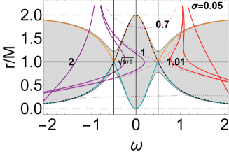
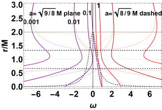
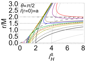
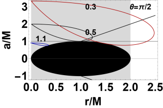
Figure 1: In all the panels, gray regions represent the ergoregion $]r_{\epsilon}^{-},r_{\epsilon}^{+}[$, a black disk corresponds to the central BH in the extended plane $r/M-a/M$, with boundary $\pm a_{\pm}$. Bottom line. Left panel: Light surfaces $r/M$, solutions of $\mathcal{L}\cdot\mathcal{L}=0$ as functions of the specific angular momentum (photon impact parameter) $\ell$. The functions $\ell_{H}^{\pm}$ are the outer and inner horizons angular momentum and the bundle origins. The curves correspond to different spins $a=\ell(r=0)$ on the equatorial plane, including BHs and NSs. The center and right panels show the metric bundles in the extended plane for selected values of the characteristic frequencies, which are marked on the curves, and for the planes $\theta=\pi/5$ (center) and $\theta=\pi/2$ (right panel). Upper line. Purple and red curves refers to the bundle frequencies $\omega_{-}$ and $\omega_{+}$, respectively. Orange and green curves represent the function $r(\omega)$ horizon curve on the extended plane.. The black dashed curve corresponds to the BH horizons as envelope surface of the bundles. Left panel: Light surfaces $r/M$ on the equatorial plane, i.e., solutions of $\mathcal{L}\cdot\mathcal{L}=0$ as functions of the bundle characteristic (photon) frequencies $\omega$ for different spins, as marked on each curve (see also bottom left panel). The center panel shows the situation on the plane $\sigma=0.6$, where $\sigma\equiv\sin^{2}\theta$. Counter-rotating orbits are also shown ($\omega<0$). Right panel: Light surfaces for different planes $\sigma$ in a NS spacetime with $a/M=\sqrt{9/8}$ (plain curves) and a BH spacetime with $a/M=\sqrt{8/9}$ (dotted curves). The BH horizons are represented as dashed horizontal lines.

The bottleneck is a region approximately around the point $r=M$ and $\omega=1/2$, that is, the extreme Kerr BH in the NS region $a\in[M,2M]$ with a further restriction in the range $a\in[M,\sqrt{9/8}M]$, which we explain in Sec. (3.1) through the analysis of replicas.

Bottleneck and angular momentum Equivalently, the bottleneck appears as a region around the point $r=M$ and $\ell=2$, where the angular momentum (and photon impact parameter) $\ell$ is related to the frequency $\omega$ through

$$\omega\equiv\frac{u^{\phi}}{u^{t}},\quad\ell\equiv\frac{L}{{E}}=-\frac{u_{\phi}}{u_{t}},\quad\ell(\omega^{\pm})=\frac{g_{\phi\phi}\omega^{\mp}}{g_{tt}},\quad\mbox{where}$$

$$\omega_{H}^{\mp}=\frac{\sqrt{2-r}}{2\sqrt{r}},\quad\mbox{and}\quad\ell_{H}^{\mp}=\frac{2r}{\sqrt{(2-r)r}}=\mathcal{A}_{0}=\frac{1}{\omega_{H}^{\mp}}.$$ (5)

In the Kerr geometry, the quantities ${E}\equiv-g_{\alpha\beta}\xi_{t}^{\alpha}u^{\beta}=-u_{t}$ and $L\equiv g_{\alpha\beta}\xi_{\phi}^{\alpha}u^{\beta}=u_{\phi}$ are constants of motion. The constant $L$ may be interpreted as the axial component of the angular momentum of a test particle following timelike geodesics and $E$ represents the total energy of the test particle coming from radial infinity, as measured by a static observer at infinity. The “horizons angular momentum” $\ell_{H}^{\pm}$ are defined as $\ell(\omega_{H}^{\pm})$, respectively. (Note the limiting condition on the energy process and $\ell=L/E=\/\omega_{H}^{\pm}$.). Evaluating these quantities on the extended plane, where the horizons are $a_{\pm}=\sqrt{r(2-r)}$ and $r=r_{g}$ is a point of the horizon curve ($r\in[0,M]$ for the inner horizons and $r\in[0,2M]$ for the outer horizons, there is $\omega^{\pm}_{H}\ell_{H}^{\pm}=1$. Bundles can also be determined by the condition $\ell=$constant. The relevant aspect is that the angular momentum of the horizon for a fixed frequency is the bundle origin $\mathcal{A}_{0}$, giving therefore a direct physical interpretation of the bundle origin.

Evaluation of the bottleneck

To analyze the bottleneck region, we could consider the distance $\Delta\omega_{\pm}=\mathbf{c}$ with $\mathbf{c}=0$ on the horizon curves $a_{\pm}$. We evaluate the minimum $\mathbf{c}$ for NSs by obtaining the solutions of $(\partial_{r}\Delta\omega_{\pm}=0)$ (or by minimizing the two points function $\omega_{+}(r_{p})-\omega_{-}(r_{m})$). On the equatorial plane, we obtain the solution

$$a_{\delta}^{\pm}\equiv\frac{1}{2}\sqrt{r\left[6+(r-3)r\pm\sqrt{(r-1)\left[r^{2}(r+3)-36\right]}\right]},$$

$$\mbox{and there is }\quad\partial_{a}\Delta\omega_{\pm}=0\quad\mbox{for}\quad a_{\delta}^{a}=\sqrt{\frac{r\left(8-r^{2}\right)}{r+2}}.$$ (6)

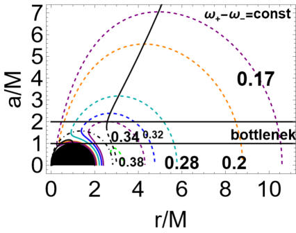
Figure 2: Upper panel: Black region represents black holes in the extended plane. Curves solutions of frequencies difference $\Delta\omega_{\pm}\equiv\omega_{+}-\omega_{-}=\mathbf{c}=$constant on the equatorial plane (curves $a=a_{z}^{\pm}$) are shown for selected values of $\mathbf{c}$ marked on the curves.The bottleneck region is highlighted. Black, black dashed, and black dotted-dashed curves are the extreme $a_{\delta}^{\pm}:\partial_{r}\Delta\omega_{\pm}=0$ (plain and dashed respectively) and $a_{\delta}^{a}:\partial_{a}\Delta\omega_{\pm}=0$ (dotted-dashed curve) of Eqs (6) (also radii $r_{\blacksquare}^{\pm}:\partial_{a}\Delta{\omega_{\pm}}=0$ and $r_{\Delta}^{\pm}(a):\partial_{r}\Delta{\omega_{\pm}}=0$ of Sec. (3)). Bottom panel: Extremes of the photon frequencies (bundles characteristic frequencies) $\omega_{\pm}$ as functions of the radius $r$, on the plane $r/M-\theta$, in the NS geometries with spin $a/M$ (dashed), marked on the curves, and BHs with spins $M/a$ (plain curves).

The analysis of the differences $\Delta\omega_{\pm}$ is indicative of the presence of bottlenecks. The extreme points of the functions $\omega(r)$ are showed also in Figs (2) and (3). Figures show the relation between BHs with spin $a/M$ and NSs with spin $M/a$. The frequencies extremes in the bottlenecks are shown in correspondence with the BH horizons.

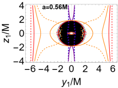
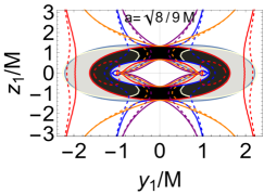
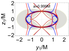
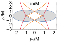
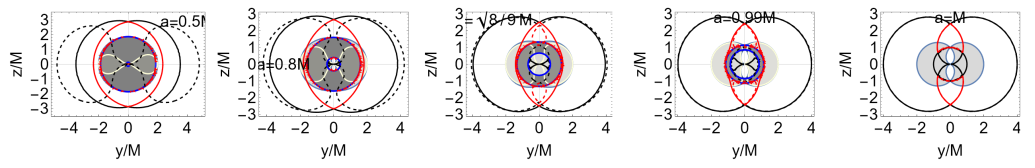
Figure 3: Upper line: Corotating and counter-rotating replicas of the Killing horizons in selected spacetimes: each panel shows the analysis for BHs with dimensionless spin, denoted on the panel, and NSs with spin $M/a$. Black region is the BH $[r_{-},r_{+}]$, where $r_{\pm}$ are the outer and inner horizons, respectively. Gray region is the ergoregion $]r_{\epsilon}^{-},r_{\epsilon}^{+}[$ in the BH spacetime, where $r_{\epsilon}^{\pm}$ are the outer and inner ergosurface, respectively. Yellow curve represent the radii $r_{\epsilon}^{\pm}$ in NSs. Plane red and blue curves are corotating replicas of the inner and outer horizons in the BH spacetime $(\omega_{H}^{\mp})$ respectively. Plane purple and orange curves are the counter-rotating replicas in the BH spacetime $(-\omega_{H}^{\mp})$. The corresponding replicas in the NS geometry are represented by dashed curves. Standard oblate spheroidal coordinates, $\left\{x_{1}\equiv\sqrt{a^{2}+r^{2}}\sin\theta\cos\phi,y_{1}\equiv\sqrt{a^{2}+r^{2}}\sin\theta\sin\phi,z_{1}\equiv r\cos\theta\right\}$, have been used. Bottom line: Extremes of the frequencies $\omega_{\pm}$ (red and black curves, respectively) as functions of the radius $r/M$ in selected BH (plain curves) with dimensionless spin $a/M$, denoted on the panel, and NS (dashed curves) with spin $M/a$. The gray region is the range $[r_{-},r_{+}]$. The radii $r_{\pm}$ are blue curves. The light-gray region is the ergoregion $]r_{\epsilon}^{-},r_{\epsilon}^{+}[$ in the BH spacetime. Yellow curves are the radii $r_{\epsilon}^{\pm}$ in the NS spacetime. There is $\{x\equiv r\sin\theta\cos\phi,y\equiv r\sin\theta\sin\phi,z\equiv r\cos\theta\}$.

We note the emergence in Figs (3) of the bottleneck region.

Effects of repulsive gravity on particles motion

The bottleneck region is characterized by repulsive gravity effects. Indeed, on the equatorial plane $(\sigma=1)$, we notice the particular radii $r_{\blacksquare}^{\pm}:\partial_{a}\Delta{\omega_{\pm}}=0$ (see corresponding solution $a_{\delta}^{a}$ of Eq. (6)), $r_{\Delta}^{\pm}(a):\partial_{r}\Delta{\omega_{\pm}}=0$ (see corresponding solution $a_{\delta}^{\pm}$ of Eq. (6)), the critical points of the separation $\Delta{\omega_{\pm}}\equiv(\omega_{+}-\omega_{-})$, and the radius $r_{\upsilon}^{\pm}$ with particle orbital energy ${E}=0$, bounding a region filled with negative energy orbits. The orbits $\hat{r}_{\pm}$, for which ${L}=0$ (ZAMOs), are also in this region. The range $]\hat{r}_{-},\hat{r}_{+}[$, is characterized by the presence of counter-rotating circular orbits–see observers ; remnants ; ergon ; Pugliese:2019efv .

From Figs (1), the spin $a_{\infty}=\sqrt{9/8}M$ emerges as a limiting spin for different planes. Near the poles ($\sigma\approx 0$) notice the closeness of the corotating and counter-rotating frequencies. The bottleneck exists in a orbital range centred around $r=M$, corresponding to critical points of the frequencies as functions of $r/M$ (for smaller spins, bottleneck can be studied by analyzing the saddle points), see also Figs (2). The NS geometries with spin $a/M>1$, where a bottleneck appears are analysed in correspondence with BHs of spin $M/a$–Figs (2). The closeness of the frequencies in the bottleneck area is also shown in Figs (2).

3.1 Horizon replicas in naked singularities

Let us introduce the following spins and limiting planes $\sigma$:

$$a_{l}\equiv 2,\quad a_{s}\equiv 1.54075,\quad a_{t}\equiv\sqrt{2},$$ (7)

$$a_{p}\equiv\sqrt{6\sqrt{3}-9}\equiv 1.17996,\quad a_{\infty}\equiv\sqrt{\frac{9}{8}},\quad\sigma_{0}\equiv\frac{1}{a^{2}\omega^{2}}$$

(the limiting plane $\sigma_{0}$ is related to the bundle origin $a_{0}\equiv 1/\omega\sqrt{\sigma}$). There can be one replica, $r_{\mathcal{Q}}^{\mathbf{I}}$, or three replicas $r_{\mathcal{Q}}^{\mathbf{III}}$, which are solutions of the equation

$$r^{4}-r^{2}\frac{a^{2}(\sigma-2)\sigma\omega^{2}+1}{\sigma\omega^{2}}+2r\frac{(a\sigma\omega-1)^{2}}{\sigma\omega^{2}}+\frac{a^{2}(\sigma-1)\left(1-a^{2}\sigma\omega^{2}\right)}{\sigma\omega^{2}}=0;$$

in the following ranges of $\sigma$

$$\mathbf{R_{m}}\equiv(]0,\sigma_{1}[\cup]\sigma_{2},1[,r_{\mathcal{Q}}^{\mathbf{I}}),(]\sigma_{1},\sigma_{2}[,r_{\mathcal{Q}}^{\mathbf{III}})$$ (8)

$$\mathbf{R_{p}}\equiv(]0,\sigma_{1}[\cup]\sigma_{2},\sigma_{0}],r_{\mathcal{Q}}^{\mathbf{I}}),(]\sigma_{1},\sigma_{2}[,r_{\mathcal{Q}}^{\mathbf{III}})$$ (9)

$$\mathbf{R_{x}}\equiv(]0,\sigma_{1}[,r_{\mathcal{Q}}^{\mathbf{I}}),(]\sigma_{1},1[,r_{\mathcal{Q}}^{\mathbf{III}})$$ (10)

$$\mathbf{R_{l}}\equiv(]0,\sigma_{1}[\cup]\sigma_{2},\sigma_{3}[,r_{\mathcal{Q}}^{\mathbf{I}}),(]\sigma_{1},\sigma_{2}[\cup]\sigma_{3},1[,r_{\mathcal{Q}}^{\mathbf{III}})$$ (11)

$$\mathbf{R_{d}}\equiv(]\sigma_{2},\sigma_{0}]],r_{\mathcal{Q}}^{\mathbf{I}})$$ (12)

$$\mathbf{R_{q}}\equiv(\sigma\in]0,1[,r_{\mathcal{Q}}^{\mathbf{I}}).$$ (13)

The limiting planes $\sigma_{1}<\sigma_{2}<\sigma_{3}$ are solutions of the equation

$$\sum_{i=0}^{6}o_{i}\sigma^{i}=0,\quad\mbox{where}$$ (14)

$$o_{6}\equiv a^{6}\omega^{6}\left(a^{2}-1\right)$$

$$o_{5}\equiv a^{4}\omega^{4}\left[4a^{3}\omega-a^{2}-\left(a^{4}+30a^{2}-27\right)\omega^{2}\right]$$

$$o_{4}\equiv a^{3}\omega^{3}\left[96a^{3}\omega^{3}-4\left(a^{4}+27\right)\omega^{2}+a\left(7a^{2}+33\right)\omega-4a^{2}\right]$$

$$o_{3}\equiv\left[8a^{5}\omega^{3}-64a^{6}\omega^{6}-6a^{2}\left(a^{4}+22a^{2}-27\right)\omega^{4}-6a^{4}\omega^{2}\right]$$

$$o_{2}\equiv a\omega\left[96a^{3}\omega^{3}-4\left(a^{4}+27\right)\omega^{2}+a\left(7a^{2}+33\right)\omega-4a^{2}\right]$$

$$o_{1}\equiv\left[4a^{3}\omega-\left(a^{4}+30a^{2}-27\right)\omega^{2}-a^{2}\right]$$

$$o_{0}\equiv a^{2}-1.$$

The limiting frequencies, $\omega_{b}$ and $\omega_{c}$, are solutions of the equations

$$a\left(a^{4}+18a^{2}-27\right)\omega^{3}+3\left(a^{2}-3\right)^{2}\omega^{2}+3a\left(a^{2}-3\right)\omega+a^{2}=0;$$

$$a\left(a^{2}+27\right)\omega^{3}+\left(3a^{2}-27\right)\omega^{2}+3a\omega+1=0;$$ (15)

respectively. Note that the equatorial plane, $\sigma=1$, the geometry $a=a_{\infty}$, and the extreme BH frequency $\omega=1/2$, are special cases. Below we provide the complete prospectus of the corotating $\omega>0$ and counter-rotating $\omega<0$ replicas of the inner and outer horizons in the extended plane, detectable in the NS geometries.

Corotating inner horizon replicas

$$a\in]1,a_{\infty}[:\left(\omega\in\left]\frac{1}{2},\omega_{b}\right[,\mathbf{R_{x}}\right),\left(\omega\in\left]\omega_{b},\frac{1}{a}\right[,\mathbf{R_{l}}\right),\left(\omega>\frac{1}{a},\mathbf{R_{p}}\right)$$

$$a\in]a_{\infty},a_{p}[:\left(\omega\in\left]\frac{1}{2},\frac{1}{a}\right[,\mathbf{R_{x}}\right),\left(\omega\in\left]\frac{1}{a},\omega_{b}\right],\mathbf{R_{d}}\right),(\omega>\omega_{b},\mathbf{R_{p}});$$

$$a\in[a_{p},a_{l}[:\left(\omega\in\left]\frac{1}{2},\frac{1}{a}\right[,\mathbf{R_{x}}\right),\left(\omega>\frac{1}{a},\mathbf{R_{d}}\right);$$

$$a\geq a_{l}:\left(\omega>\frac{1}{2},\mathbf{R_{d}}\right).$$ (16)

Corotating outer horizon replicas

$$a\in]1,a_{l}]:\left(\omega\in\left]0,\frac{1}{2}\right[,\mathbf{R_{x}}\right);$$

$$a>a_{l}:\left(\omega\in\left]0,\frac{1}{a}\right[,\mathbf{R_{x}}\right),\left(\omega\in\left]\frac{1}{a},\frac{1}{2}\right[,\mathbf{R_{d}}\right).$$ (17)

Counter-rotating outer horizon replicas

$$a\in]1,a_{s}]:\left(\omega\in\left]-\frac{1}{2},\omega_{c}\right[,\mathbf{R_{m}}\right),(\omega\in]\omega_{c},0[,\mathbf{R_{x}});$$ (18)

$$a\in]a_{s},a_{l}]:\left(\omega\in\left]-\frac{1}{2},\omega_{b}\right],\mathbf{R_{q}}\right),(\omega\in]\omega_{b},\omega_{c}[,\mathbf{R_{m}}),$$

$$\qquad\qquad\quad(\omega\in]\omega_{c},0[,\mathbf{R_{x}});$$

$$a>a_{l}:\left(\omega\in\left]-\frac{1}{2},-\frac{1}{a}\right[,\mathbf{R_{d}}\right),\left(\omega\in\left[-\frac{1}{a},\omega_{b}\right],\mathbf{R_{q}}\right),$$

$$\qquad\quad(\omega\in]\omega_{b},\omega_{c}[,\mathbf{R_{m}}),(\omega\in]\omega_{c},0[,\mathbf{R_{x}});$$

Counter-rotating inner horizon replicas

$$a\in]1,a_{p}]:\left(\omega<-\frac{1}{a},\mathbf{R_{p}}\right),\left(\omega\in\left]-\frac{1}{a},-\frac{1}{2}\right[,\mathbf{R_{m}}\right);$$

$$a\in]a_{p},a_{t}[:(\omega\leq\omega_{b},\mathbf{R_{d}}),\left(\omega\in\left]\omega_{b},-\frac{1}{a}\right[,\mathbf{R_{p}}\right),\left(\omega\in\left[-\frac{1}{a},-\frac{1}{2}\right[,\mathbf{R_{m}}\right);$$

$$a\in]a_{t},a_{s}[:\left(\omega<-\frac{1}{a},\mathbf{R_{d}}\right),\left(\omega\in\left[-\frac{1}{a},\omega_{b}\right],\mathbf{R_{q}}\right),\left(\omega\in\left]\omega_{b},-\frac{1}{2}\right[,\mathbf{R_{m}}\right);$$

$$a\in[a_{s},a_{l}]:\left(\omega<-\frac{1}{a},\mathbf{R_{d}}\right),\left(\omega\in\left[-\frac{1}{a},-\frac{1}{2}\right[,\mathbf{R_{q}}\right);$$

$$a>a_{l}:\left(\omega<-\frac{1}{2},\mathbf{R_{d}}\right).$$ (19)

Examples of replicas are shown in Figs (3). Replicas ranges are more articulated, as expected, in the counter-rotating case and for the inner horizon replicas. There is a limiting frequency $1/a$, which is related to the bundle origin and the horizon angular momentum $\ell$. Furthermore, it frames the correspondence between NSs with spins $a/M$ and NSs with spin $M/a$.

4 Conclusion

In this work, we presented evidences of repulsive gravity effects in Kerr naked singularities by analyzing photon orbits, replicas and bottlenecks–Sec. (3.1). Replicas, photon orbits with frequency $\omega$ (bundles characteristic frequency) equal in magnitude with the BHs inner and outer horizons, can extract “information" on the inner horizon frequencies near the poles ($\sigma\approx 0$): close to the rotational axis $\sigma\ll 1$, for a spacetime $a$ it is possible to find an inner horizon replica in the outer region $r>r_{+}$. We completed the analysis of the corotating and counter-rotating (inner and outer) horizons replicas. We showed the correspondence between BH and NS through the frequencies $\omega$, framed in the metric bundles approach of Sec. (3)–Figs (1). Bottlenecks appear as a restriction of the area of the plane $r-\omega$ or $r-\ell$ (angular momentum of the horizon and photon impact parameter) defined by light surfaces, as a characteristic of slowly spinning NSs, which in the BH case coincide with the Killing horizons; therefore, bottlenecks are also defined as horizon remnants.

The bottleneck analysis shows also the correspondence between NSs with dimensionless spin $a/M$ and BHs with spin $M/a$, a BH-NS dualism. The ratio is related to the bundle frequency and angular momentum–Figs (3).

References

- (1) D. Pugliese&H. Quevedo, Eur. Phys. J. C 81 3 (2021) 258.
- (2) D. Pugliese&H. Quevedo, Eur. Phys. J. C 78 1 (2018) 69.
- (3) D. Pugliese&H. Quevedo, Eur. Phys. J. C 79 3 (2019) 209.
- (4) D. Pugliese&H. Quevedo, arXiv:1910.02808 [gr-qc] (2019).
- (5) D. Pugliese&H. Quevedo, arXiv:1910.04996 [gr-qc] (2019).
- (6) D. Pugliese& G. Montani, Entropy 22 (2020) 402.
- (7) D. Pugliese & Z. Stuchlik, Class.Quant.Grav. https://doi.org/10.1088/1361-6382/abff97 (2021).
- (8) V. S. Manko&E. Ruiz, Phys. Lett. B. 791 (2019) 26–29.
- (9) The Event Horizon Telescope Collaboration et al., ApJL 875 (2019) L1.
- (10) F. de Felice, Mont. Notice R. astr. Soc 252 (1991) 197–202.
- (11) F. de Felice and S. Usseglio-Tomasset, Class.Quant.Grav. 8 (1991) 1871–1880.
- (12) F. de Felice&S. Usseglio-Tomasset, Gen.Rel.Grav. 24 (1992) 10.
- (13) F. de Felice and Y. Yunqiang, Class.Quant.Grav. 10 (1993) 353–364.
- (14) F. de Felice and L. Di G. Sigalotti, Ap.J. 389 (1992) 386–391.
- (15) C. Chakraborty, M. Patil, et al., Phys.Rev.D 95 8 (2017) 084024.
- (16) I. V. Tanatarov and O. B. Zaslavskii, Gen.Rel.Grav. 49 9 (2017) 119.
- (17) S. Mukherjee and R. K. Nayak, Astrophys. Space Sci. 363 8 (2018) 163.
- (18) O. B Zaslavskii., Phys.Rev.D 98 10 (2018) 104030.
- (19) O. B. Zaslavskii, Phys.Rev.D 100 2 (2019) 024050.
- (20) F. de Felice, A&A45 (1975) 65.
- (21) D. Batic, D. Chin, M. Nowakowski, Eur.Phys.J.C 71 (2011) 1624.
- (22) O. Luongo&H. Quevedo, Phys.Rev.D 90 (2014) 084032.
- (23) M. Patil, P. S. Joshi and D. Malafarina, Phys.Rev.D 83 (2011) 064007.
- (24) J. W. Maluf, Gen. Rel. Grav. 46 (2014) 1734.
- (25) Z. Stuchlik, Bull. Astron. Inst. Czech 31 (1980) 129.
- (26) J. Gariel, N. O. Santos and J. Silk, Phys.Rev.D 90 (2014) 063505.
- (27) N. Pelavas, N. Neary and K. Lake, Class.Quant.Grav. 18 (2001) 1319.
- (28) C. Herdeiro and E. Radu, Phys.Rev.D 89 (2014) 1240 18.
- (29) Z. Stuchlik, D. Pugliese, J. Schee & H. Kucáková, Eur. Phys. J. C 75 9 (2015) 451.
- (30) A. V. Frolov and V. P. Frolov, Phys.Rev.D 90 12 (2014) 124010.
- (31) M. B. Paranjape, Physics Today, in Commentary&Reviews 24 May 2017.
- (32) R. Goswami, P. S. Joshi and P. Singh, Phys.Rev.Lett. 96 (2006) 031302.
- (33) C. Vaz&L. Witten, Phys.Lett.B 442 (1998) 90.
- (34) H. Iguchi, T. Harada and K. i. Nakao, Prog. Theor. Phys. 101 (1999) 1235.
- (35) H. Iguchi, K. i. Nakao and T. Harada, Phys.Rev.D 57 (1998) 7262.
- (36) H. Iguchi, T. Harada and K. I. Nakao, Prog. Theor. Phys. 103 (2000) 53.
- (37) M. J. Lake&B. Carr, JHEP 1511 (2015) 105.
- (38) B. J. Carr, arXiv:1703.08655 [gr-qc].
- (39) B. J. Carr, J. Mureika and P. Nicolini, JHEP 1507 (2015) 052.
- (40) B. J. Carr, Springer Proc. Phys. 170 (2016) 159.
- (41) Y. Prok et al. [CLAS Collaboration], Phys.Lett.B 672 (2009) 12.
- (42) D. Pugliese, H. Quevedo, J. A. Rueda H. and R. Ruffini, Phys.Rev.D 88 (2013) 024053.
- (43) R. Ruffini and S. Bonazzola, Phys. Rev. 187 (1969) 1767.
- (44) D. Pugliese, H. Quevedo and R. Ruffini, Phys.Rev.D 83 (2011) 104052.
- (45) D. Pugliese, H. Quevedo and R. Ruffini, Eur. Phys. J. C 77 4 (2017) 206.
- (46) D. Pugliese, H. Quevedo and R. Ruffini, Phys.Rev.D 88 (2013) 024042.
- (47) D. Pugliese, H. Quevedo and R. Ruffini, Phys.Rev.D84 (2011) 044030.
- (48) D. Pugliese, H. Quevedo and R. Ruffini, Phys. Rev. D 83 (2011) 024021.
- (49) B. Carr, H. Mentzer, J. Mureika, P. Nicolini, Eur.Phys.J. C 80 (2020) 1166.
- (50) C. Sivaram and K. P. Sinha, Phys. Rev. D 16 (1977) 1975.
- (51) A. Salam and J.A. Strathdee, Phys. Rev. D 18 (1978) 4596.
- (52) C. F. E. Holzhey and F. Wilczek, Nucl. Phys. B 380 (1992) 447.
- (53) R.L. Oldershaw and J. Cosmol. 6 (2010) 1361.
- (54) B.J. Carr, Mod. Phys. Lett. A 28 (2013) 1340011.
- (55) V. Cardoso, P. Pani, M. Cadoni and M. Cavaglia, Phys.Rev.D 77 (2008) 124 044.
- (56) N. Comins& B. F. Schutz, Proc. R. Soc. A 364 1717 (1978) 211–226.
- (57) A. Helou, I. Musco, J. C. Miller, Class.Quant.Grav. 34 13 (2017) 135012.
- (58) R. Penrose, Nuovo Cimento Rivista Serie (1969) 1.
- (59) S. L. Shapiro& S. A. Teukolsky, American Scientist 79 4 (1991) 330–343.
- (60) T. Crisford and J. E. Santos, Phys. Rev. Lett. 118 (2017) 181101.
- (61) A. Loeb, In Search of Naked Singularities Scientific American Observations-Opinion May 3 (2020).
- (62) P. S. Joshi, Scientific American 300 2 (2009) 36–43.
- (63) T. Harada, Pramana 63 4 (2004) 741–753.
- (64) R. Penrose, JJApA 20 (1999) 233.
- (65) P. S. Joshi, N. Dadhich& R. Maartens, Phys.Rev.D 65 (2002) 101501.
- (66) S. L. Shapiro and S. A. Teukolsky, Philosophical Transactions: Physical Sciences and Engineering 340 1658 (1992) 365–390.
- (67) B. K. Berger, Living Reviews in Relativity 5 1 (2002) 1.
- (68) R. Bousso, A. Shahbazi–Moghaddam, M. Tomasevic, Phys.Rev.D 100 (2019) 126010.
- (69) A. H. Ziaie, A. Ranjbar& H. R. Sepangi, Class. Quant. Grav. 32 (2015) 025010.
- (70) P. S. Joshi, Gravitational Collapse and Spacetime Singularities, Cambridge Monographs on Mathematical Physics, New York (2007).
- (71) R. M. Wald and V. Iyer, Phys.Rev.D 44 (1991) 3719.
- (72) S. L. Shapiro& S. A. Teukolsky, Phys. Rev. Lett. 66 (1991) 994.
- (73) T. A. Apostolatos& K. S. Thorne,Phys. Rev. D 46 (1992) 2435.
- (74) T. Jacobson& T. P. Sotiriou, Phys. Rev. Lett. 103 (2009) 141101.
- (75) T. Jacobson& T. P. Sotiriou, J. Phys. Conf. Ser. 222 (2010) 012041.
- (76) E. Barausse, V. Cardoso, G. Khanna, Phys.Rev.Lett.105 (2010) 261102.
- (77) B. Giacomazzo, L. Rezzolla, N. Stergioulas, Phys.Rev.D 84 (2011) 024022.
- (78) R. M. Wald, Class.Quant.Grav. 16 (1999) A177.
- (79) R. M. Wald, Living Rev. Relativ. 4(1) (2001) 6.
- (80) D. Pugliese and H. Quevedo, 2021, to be submitted
- (81) P. T. Chrusciel, J.Lopes Costa& M. Heusler, Living Rev. Rel. 15 (2012) 7.
- (82) Z. Li and C. Bambi, Phys.Rev.D 87, 124022 (2013).
- (83) D. Pugliese and H. Quevedo, Eur. Phys. J. C 75 5 (2015) 234.