Locally Adaptive Algorithms for Multiple Testing with Network Structure, with Application to Genome-Wide Association Studies

Abstract

Linkage analysis has provided valuable insights to the GWAS studies, particularly in revealing that SNPs in linkage disequilibrium (LD) can jointly influence disease phenotypes. However, the potential of LD network data has often been overlooked or underutilized in the literature. In this paper, we propose a locally adaptive structure learning algorithm (LASLA) that provides a principled and generic framework for incorporating network data or multiple samples of auxiliary data from related source domains; possibly in different dimensions/structures and from diverse populations. LASLA employs a $p$-value weighting approach, utilizing structural insights to assign data-driven weights to individual test points. Theoretical analysis shows that LASLA can asymptotically control FDR with independent or weakly dependent primary statistics, and achieve higher power when the network data is informative. Efficiency again of LASLA is illustrated through various synthetic experiments and an application to T2D-associated SNP identification.

1 Introduction

1.1 Multiple testing for network data

Statistical analysis of network-structured data is an important topic with a wide range of applications. Our study is motivated by genome-wide association studies (GWAS), where a primary objective is to identify disease-associated single-nucleotide polymorphisms (SNPs) across diverse populations. Recent studies have indicated that linkage analysis can provide insights into the genetic basis of complex diseases, particularly SNPs in linkage disequilibrium (LD) can jointly contribute to the representation of the disease phenotype [1]. However, existing research in GWAS has often neglected the LD network information, representing a significant limitation. This article aims to address this gap by developing integrative analytical tools that combine GWAS association data with LD network information for more efficient identification of disease-associated SNPs.

Let $m$ denote the number of SNPs and $[m]=\{1,\ldots,m\}$. The primary data, as provided by GWAS, consists of a list of test statistics $\boldsymbol{T}=\{T_{i}:i\in[m]\}$, which assess the association strength of individual SNPs with a phenotype of interest. Let $\boldsymbol{P}=\{P_{i}:i\in[m]\}$ denote the corresponding $p$-values. The auxiliary data, as provided by linkage analysis, is a matrix $\boldsymbol{S}=(r_{ij}:i,j\in[m])$ comprising pairwise correlations, where $r_{ij}$ measures the LD correlation between SNP $i$ and SNP $j$. To illustrate, we construct an undirected LD graph based on pairwise LD correlation in Figure 1.1, where each node represents a SNP and an edge is drawn to connect two SNPs if their correlation exceeds a pre-determined cutoff.

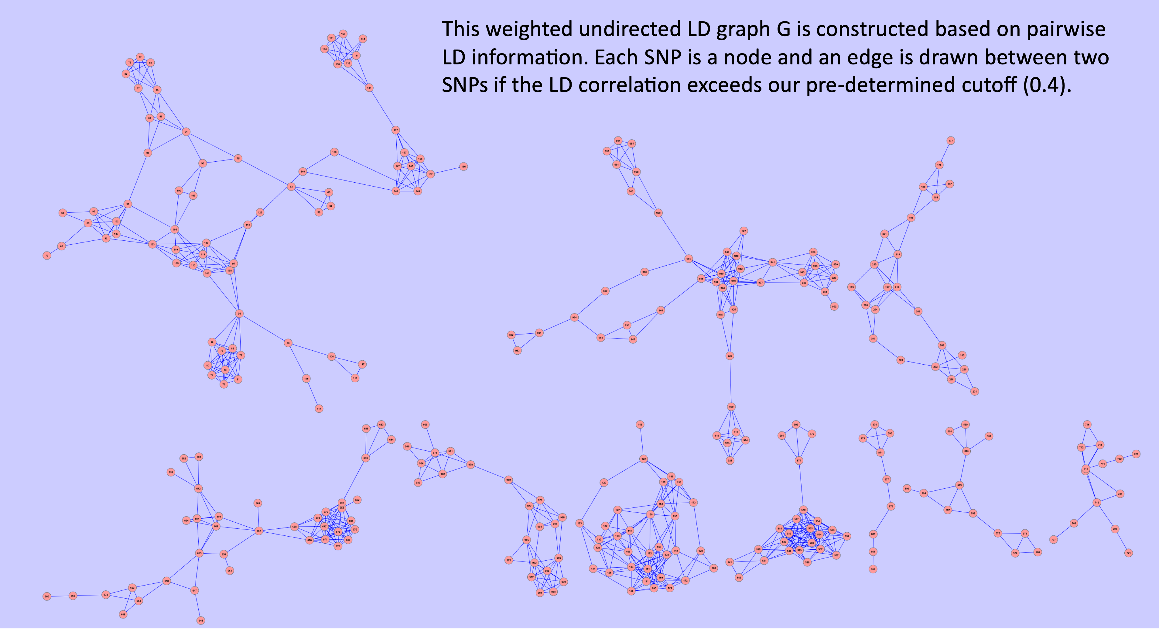
Figure 1.1: Auxiliary linkage data provide structural information that can be utilized to identify significant SNPs.

Incorporating LD patterns into inference is desirable in GWAS as it can improve the power and interpretability of analysis. However, developing a principled approach that cross-utilizes data from different sources is a challenging task. Firstly, the primary data $\boldsymbol{T}$ and the auxiliary data $\boldsymbol{S}$ are usually collected from different populations. For instance, in our analysis detailed in Section 5, the target population in GWAS consists of 77,418 individuals with Type 2 diabetes, while the auxiliary data for linkage analysis are collected from the general population [1000 Genomes (1000G) Phase 3 Database]. Secondly, the dimensions of $\boldsymbol{T}$ and $\boldsymbol{S}$ do not match coordinate by coordinate as in the conventional settings. Specifically, $\boldsymbol{T}$ is a vector of statistics while $\boldsymbol{S}$ is an LD matrix.

Motivated by the observation that SNPs in the same sub-network can exhibit similar distributional characteristics and tend to work together in GWAS [1], this article develops a class of locally adaptive structure learning algorithms (LASLA) that is capable of incorporating side information in different dimensions and from diverse populations. LASLA reflects this structural knowledge by computing a set of locally adaptive weights $\{w_{i}:i\in[m]\}$ to adjust the $p$-values $\{P_{i}:i\in[m]\}$. In summary, LASLA follows a two-step strategy:

Step 1: Learn the relational or structural knowledge of the high-dimensional parameter through auxiliary data.

Step 2: Apply the structural knowledge by adaptively placing differential weights $w_{i}$ on $p$-values $P_{i}$, for $i\in[m]$.

1.2 Related work and our contribution

Structured multiple testing has gained increasing attention in recent years [2, 3, 4, 5, 6]. The fundamental idea is to supplement the sequence of primary statistics $\boldsymbol{T}=\{T_{i}:i=1,2,\ldots\}$, such as $z$-values, with an auxiliary sequence $\boldsymbol{U}=\{U_{i}:i=1,2,\ldots\}$ to enhance the power of inference. The auxiliary data can be collected in various ways, including (a) externally from prior studies and secondary data sources ([7, 8]); (b) internally within the same data using carefully constructed independent sequences ([3, 9]); and (c) intrinsically through patterns associated with the data, such as the natural order of data streams ([10, 2]) or spatial locations ([11, 12]).

Aforementioned studies primarily focus on an auxiliary sequence $\boldsymbol{U}$ that has the same dimension as $\boldsymbol{T}$, while the exploration of more generalized side information such as LD matrices or multiple auxiliary sequences remains limited. Moreover, existing structure-adaptive methods ([3, 4, 9]) have dominantly relied on leveraging the sparsity structure encoded in auxiliary data, while recent research has revealed that other forms of structural information, including signal amplitudes, heteroscedasticity, and hierarchical structures, can also provide valuable insights ([13, 14, 15]). In the context of GWAS, where SNPs from different subnetworks may exhibit distinct distributional characteristics, this broader range of structural information becomes particularly relevant.

Our contributions are three-fold. First, we introduce a systematic approach for learning network side information through a distance matrix to be discussed in Section 2.1. In addition to network data, our framework can incorporate various types of side information, regardless of the data dimension (see Section S1 in the Supplementary Material). Second, LASLA leverages both the sparsity and distributional information by computing weights motivated by a hypothetical oracle ([16, 17]); thereby offers greater power improvement when compared to existing techniques [18, 19, 12]. Lastly, our theoretical analysis shows that LASLA asymptotically controls False Discovery Rate (FDR) and False Discovery Proportion (FDP) for both independent and weakly dependent primary statistics, along with proven power gain under mild conditions.

2 Locally Adaptive Structure Learning Algorithms

2.1 Problem Formulation and Basic Framework

Suppose we are interested in testing $m$ hypotheses:

$${H_{0,i}}:\theta_{i}=0\quad\text{vs.}\quad H_{1,i}:\theta_{i}=1,\quad i\in[m],$$ (2.1)

where $\boldsymbol{\theta}=(\theta_{i}:i\in[m])$ is a vector of binary random variables indicating the existence or absence of signals at the testing locations. A multiple testing rule can be represented by a binary vector $\boldsymbol{\delta}=(\delta_{i}:i\in[m])\in\{0,1\}^{m}$, where $\delta_{i}=1$ indicates that we reject $H_{0,i}$ and $\delta_{i}=0$ otherwise. This article focuses on problem (2.1) with the goal of controlling the FDP and FDR [20] defined respectively by:

$$\text{FDP}(\boldsymbol{\delta})=\frac{\sum_{i=1}^{m}(1-\theta_{i})\delta_{i}}{\max(\sum_{i=1}^{m}\delta_{i},1)},\quad\text{and FDR}=\mathbb{E}\left\{\text{FDP}(\boldsymbol{\delta})\right\}.$$

An ideal procedure should maximize power, which is interpreted as the expected number of true positives:

$$\text{ETP}=\Psi(\boldsymbol{\delta})=\mathbb{E}\left\{\sum_{i=1}^{m}\theta_{i}\delta_{i}\right\}.$$

Our approach involves the calculation of a distance matrix $\boldsymbol{D}=(1-r^{2}_{ij}:i,j\in[m])$ based on the LD matrix $\boldsymbol{S}=(r^{2}_{ij}:i,j\in[m])$, where $r_{ij}\in[0,1]$ represents the Pearson’s correlation coefficient that measures the linkage disequilibrium between SNPs $i$ and $j$. Note that the distance matrix $\boldsymbol{D}$ contains identical information as $\boldsymbol{S}$ but it facilitates our definition of the local neighborhood and subsequent data-driven algorithms. Specifically, SNPs with higher correlation $r_{ij}$ are considered “closer” in distance. Clusters of SNPs with small pairwise distance form a local neighborhood which may exhibit distinct distributional patterns compared to the far-away neighborhoods. The derivation of a distance matrix $\boldsymbol{D}$ from the network auxiliary data $\boldsymbol{S}$ is straightforward. However, it becomes more challenging when dealing with generalized side information. An extension on how to define a proper distance matrix for general side information is discussed in Section S2 of the Supplementary Material. Intuitively, leveraging the local heterogeneity can enhance the interpretability and power of multiple testing procedures. This motivates us to propose LASLA discussed in the next a few sections.

2.2 Oracle FDR procedure

The weighting strategy provides an effective approach to incorporating relevant domain knowledge in multiple testing and has been widely used in the literature ([21, 22, 8]; among others). The proposed LASLA builds upon this strategy. We first introduce an oracle procedure in this section under an ideal setting. Then in Sections 2.3–2.4, we develop a data-driven algorithm that emulates the oracle and leverages the distance matrix to construct informative weights.

Assume the primary test statistics $\{T_{i}:i\in[m]\}$ follow a hierarchical model:

$$\theta_{i}\overset{\text{ind}}{\sim}\text{Bernoulli}(\pi_{i}^{*}),\quad{\mathbb{P}}(T_{i}\leq t|\theta_{i})=(1-\theta_{i})F_{0}(t)+\theta_{i}F_{1i}^{*}(t).$$ (2.2)

We would like to make two remarks to clarify our notations. Firstly, (2.2) is not intended to exactly correspond to the true data-generating process. Instead, it serves as a hypothetical model to motivate the use of our data-driven weights. Secondly, we use $\pi_{i}^{*}$ and $F_{1i}^{*}(t)$ to account for the potential heterogeneity in the distribution across various testing units in light of full auxiliary information $\mathcal{D}_{i}$ that will be specified in Section 2.3. By contrast, the null distribution $F_{0}(t)$ is known and identical for all testing units. Denote by

$$F_{i}^{*}(t)=(1-\pi_{i}^{*})F_{0}(t)+\pi_{i}^{*}F_{1i}^{*}(t)$$ (2.3)

the mixture distribution and $f_{i}^{*}(t)$ the corresponding density. The optimal testing rule, which has the largest ETP among all valid marginal FDR/FDR procedures ([16, 3, 17]), is a thresholding rule based on the local false discovery rate (lfdr):

$$L_{i}^{*}={\mathbb{P}}(\theta_{i}=0|T_{i})={(1-\pi_{i}^{*})f_{0}(T_{i})}/{f_{i}^{*}(T_{i})}.$$

A step-wise algorithm (e.g. [16]) can be used to determine a data-driven threshold along the $L_{i}^{*}$ ranking. Specifically, denote by $L_{(1)}^{*}\leq\ldots\leq\ L_{(m)}^{*}$ the sorted $L_{i}^{*}$ values, and $H_{(1)},\ldots,H_{(m)}$ the corresponding hypotheses. Let $k_{*}=\max\left\{j:j^{-1}\sum^{j}_{i=1}{L_{(i)}^{*}\leq\alpha}\right\}.$ Then the stepwise algorithm rejects $H_{(1)},\ldots,H_{(k_{*})}$.

2.3 A data-driven procedure

Note that, $\pi_{i}^{*}$ and $f_{i}^{*}(t)$ are hypothetical and non-accessible oracle quantities that cannot be directly utilized in the data-driven algorithms. Therefore, we use kernel estimation to approximate the oracle quantities. By convention, throughout we assume that $\theta_{j}$ does not affect the null distribution of $T_{i}$ for $i\neq j$. Let $\boldsymbol{D}_{i}$ be the $i$th column of $\boldsymbol{D}$. Adapting the fixed-domain asymptotics in [23], we define $\mathcal{D}_{i}$ as a continuous finite domain (w.r.t. coordinate $i$) in $\mathbb{R}$ with positive measure, where each $d\in\mathcal{D}_{i}$ is a distance and $0\in\mathcal{D}_{i}$. The two sets $\boldsymbol{D}_{i}$ and $\mathcal{D}_{i}$ can be viewed as distances measured from a partial/full network, respectively, and $\boldsymbol{D}_{i}\subset\mathcal{D}_{i}$. The details on the fixed-domain asymptotics, i.e., $\boldsymbol{D}_{i}\rightarrow\mathcal{D}_{i}$ as $m\rightarrow\infty$, are relegated to Section S7 in the Supplementary Material.

The approximation of $\pi_{i}^{*}$ is inspired by the screening process in [12]. We reiterate the essence here for completeness. Let $\mathcal{D}_{ij}$ be the distance between entries $i$ and $j$ from the full network. A key assumption is that $\pi_{i}^{*}$ is close to $\pi_{j}^{*}$ if $\mathcal{D}_{ij}$ is small, which enables us to resemble $\pi_{i}^{*}$ using neighboring points. Since a direct evaluation of $\pi_{i}^{*}$ is challenging, we consider an intermediate quantity:

$$\pi_{i}^{\tau}=1-\frac{\mathbb{P}(P_{i}>\tau\mid\mathcal{D}_{i})}{1-\tau},\quad 0<\tau<1,$$

which offers a good approximation of $\pi_{i}^{*}$ with a suitably chosen $\tau$. Intuitively, when $\tau$ is large, null $p$-values are dominant in the tail area $[\tau,1]$. Hence $\mathbb{P}(P_{i}>\tau\mid\mathcal{D}_{i})/(1-\tau)$ approximates the overall null proportion. See [12] for more discussion. Let $K$: $\mathbb{R}\rightarrow\mathbb{R}$ be a positive, bounded, and symmetric kernel function that satisfies the following conditions:

$$\int_{\mathbb{R}}K(x)dx=1,\quad\int_{\mathbb{R}}xK(x)dx=0,\quad\int_{\mathbb{R}}x^{2}K(x)dx=\sigma_{K}^{2}<\infty.$$ (2.4)

Define $K_{h}(x)=h^{-1}K(x/h)$, where $h$ is the bandwidth, and $V_{h}(i,j)=K_{h}(D_{ij})/K_{h}(0)$. We can view $m_{i}=\sum_{j\neq i}V_{h}(i,j)$ as the total “mass” in the vicinity of $i$. Suppose we want to count how many null $p$-values are greater than $\tau$ among the $m_{i}$ observation around $i$. The empirical count is given by $\sum_{j\neq i}V_{h}(i,j)\mathbb{I}(P_{j}>\tau)$, whereas the expected count can be approximated by $m_{i}(1-\pi_{i}^{\tau})(1-\tau)$. Setting equal the expected and empirical counts, we construct a data-driven quantity that resemble $\pi_{i}^{\tau}$, $i\in[m]$ by :

$$\pi_{i}=1-\frac{\sum_{j\neq i}\left[{V_{h}(i,j){\mathbb{I}}\{P_{j}>\tau\}}\right]}{(1-\tau)\sum_{j\neq i}{V_{h}(i,j)}}.$$ (2.5)

Similarly, we introduce a data-driven quantity that resemble the hypothetical density $f_{i}^{*}(t)$ for $i\in[m]$ by:

$$f_{i}(t)=\frac{\sum_{j\neq i}\left[{V_{h}(i,j)K_{h}(T_{j}-t)}\right]}{\sum_{j\neq i}{V_{h}(i,j)}},$$ (2.6)

which describes the likelihood of $T_{i}$ taking a value in the vicinity of $t$. Consequently, the data-driven lfdr is given by:

$$L_{i}=\{1-\pi_{i}\}f_{0}(T_{i})/f_{i}(T_{i}).$$ (2.7)

Let $L_{(1)}\leq\ldots\leq L_{(m)}$ denote the sorted values of $L_{i}$. Following the approach in Section 2.2, we choose $L_{(k)}$ to be the threshold, where $k=\max\{j:j^{-1}\sum^{j}_{i=1}{L_{(i)}\leq\alpha}\}$.

2.4 Oracle-assisted weights

Assume for now that $T_{i}$ is independent of $\boldsymbol{T}_{-i}=\{T_{j},j\in[m],j\neq i\}$. This assumption is only used to motivate the methodology and is not required for theoretical analysis. We assume that $f_{0}$ is symmetric about zero; otherwise we can always transform the primary statistics into $z$-statistics/$t$-statistics, etc. We now introduce the weights mimicking the oracle procedure above.

Intuitively, the thresholding rule $L_{i}<t$ is approximately equivalent to the following rule:

$$T_{i}<t_{i}^{-}\text{ or }T_{i}>t_{i}^{+}.$$ (2.8)

Here $t_{i}^{-}\leq 0$ and $t_{i}^{+}\geq 0$ are coordinate-specific thresholds that lead to asymmetric rejection regions, which are useful for capturing structures of the alternative distribution, such as unequal proportions of positive and negative signals [16, 4, 15].

The next step is to derive weights that can emulate the rule (2.8). We first consider the case of $T_{i}\geq 0$. Let $t^{+}_{i}=\infty$ if $(1-\pi_{i})f_{0}(t)/f_{i}(t)>L_{(k)}\text{ for all }t\geq 0,$ else we let

$$t^{+}_{i}=\inf\left[t\geq 0:\{(1-\pi_{i})f_{0}(t)/f_{i}(t)\}\leq L_{(k)}\right]$$ (2.9)

The rejection rule $T_{i}>t_{i}^{+}$ is equivalent to the $p$-value rule $P_{i}<1-F_{0}(t_{i}^{+})$, where $P_{i}$ is the one-sided $p$-value and $F_{0}$ is the null distribution of $T_{i}$. Define the weighted $p$-values as $\{P_{i}^{w}=P_{i}/w_{i}:i\in[m]\}$. If we choose a universal threshold for all $P_{i}^{w}$, then using weight $w_{i}=1-F_{0}(t^{+}_{i})$ can effectively emulate $T_{i}>t_{i}^{+}$.

For the case of $T_{i}<0$, let $t^{-}_{i}=-\infty$ if $(1-\pi_{i})f_{0}(t)/f_{i}(t)>L_{(k)}\text{ for all }t\leq 0,$ else we let

$$t^{-}_{i}=\sup\left[t\leq 0:\{(1-\pi_{i})f_{0}(t)/f_{i}(t)\}\leq L_{(k)}\right]$$ (2.10)

The corresponding weight is given by $w_{i}=F_{0}(t^{-}_{i})$.

To ensure the robustness of the algorithm, we set $w_{i}=\max\{w_{i},\xi\}$ and $w_{i}=\min\{w_{i},1-\xi\}$, where $0<\xi<1$ is a small constant. In all numerical studies, we set $\xi=10^{-5}$. To expedite the calculation and facilitate our theoretical analysis, we propose to use only a subset of $p$-values in the neighborhood to obtain $\pi_{i}$ and $f_{i}(t)$ for $i\in[m]$. Specifically, we define $\mathcal{N}_{i}=\{j\neq i:D_{ij}\leq a_{\epsilon}\}$ as a neighborhood set which only contains indices with distance to $i$ smaller than $a_{\epsilon}$ and satisfies $|\mathcal{N}_{i}|=m^{1-\epsilon}$ for some small constant $\epsilon>0$. Moreover, we require that $D_{ij_{1}}\leq D_{ij_{2}}$ for any $j_{1}\in\mathcal{N}_{i}$, $j_{2}\notin\mathcal{N}_{i}$, and $j_{2}\neq i$. This approach has minimal impact on numerical performance, as $p$-values that are far apart contribute little.

Furthermore, for each $i\in[m]$, we propose to compute an index-dependent oracle $L^{i}_{(k)}$ which only relies on $|\mathcal{N}_{i}|$ statistics as opposed to the universal threshold $L_{(k)}$ defined in Section 2.3. This modification arises from the subtle fact that, though $L_{i}$ in (2.7) is estimated without using $T_{i}$ itself, $w_{i}$ still correlates with $T_{i}$ since the determination of $k$ in the universal threshold relies on all primary statistics. This intricate dependence structure poses challenges for the theoretical analysis. Therefore, we compute the index-dependent threshold $L^{i}_{(k)}$ to ensure that $w_{i}$ is independent of $T_{i}$ under the null hypothesis at the cost of computational efficiency. We summarize the proposed method in Algorithm 1, and prove that the corresponding weighted multiple testing strategy is asymptotically valid in Section 3.1.

Algorithm 1 Oracle-assisted weights

1:  Input: FDR level $\alpha$, $\epsilon$ specifying the size of the sub-neighborhood, kernel function $K(\cdot)$.

2:  Input: Primary statistics $\boldsymbol{T}=\{T_{i}:i\in[m]\}$ and distance matrix $\boldsymbol{D}=(D_{ij}:i,j\in[m])$.

3:  For $i\in[m]$ do:

4:    For $j\in\mathcal{N}_{i}$ do:

5:      Estimate $\pi^{i}_{j}$ by (2.5) with the summation taken over $\mathcal{N}_{i}$.

6:      Estimate $f^{i}_{j}(t)$ by (2.6) with the summation taken over $\mathcal{N}_{i}$.

7:      Compute $L^{i}_{j}$ as given by (2.7) with $\pi_{j}$ replaced by $\pi^{i}_{j}$; $f_{j}(t)$ by $f^{i}_{j}(t)$.

8:    Denote the sorted statistics by $L^{i}_{(1)}\leq\ldots\leq L^{i}_{(|\mathcal{N}_{i}|)}$.

9:    Choose $L^{i}_{(k)}$ to be the oracle threshold, where $k=\max\{j\in[|\mathcal{N}_{i}|]:j^{-1}\sum^{j}_{l=1}{L^{i}_{(l)}\leq\alpha}\}$.

10:    If $T_{i}\geq 0$ then:

11:      Compute $t^{+}_{i}$ as given by (2.9), with $L_{(k)}$ replaced by $L^{i}_{(k)}$;

12:      Compute the weight by $w_{i}=1-F_{0}(t^{+}_{i})$.

13:    If $T_{i}<0$ then:

14:      Compute $t^{-}_{i}$ as given by (2.10), with $L_{(k)}$ replaced by $L^{i}_{(k)}$.

15:      Compute the weight by $w_{i}=F_{0}(t^{-}_{i})$.

16:  Output: Oracle-assisted weights $\{w_{i}:i\in[m]\}$.

Alternatively, a computationally much more efficient procedure that utilizes the universal oracle threshold $L_{(k)}$ for all $i\in[m]$ is introduced in Algorithm S2 of Section S4 in the Supplementary Material. We remark on the distinctions between these two algorithms. Theoretically, the weighted multiple testing procedure based on Algorithm 1 can achieve asymptotic FDR and FDP control with minimal assumptions as shown in Section 3.1, but the validity of the alternative procedure based on Algorithm S2 requires more technical assumptions, as discussed in Section S7 of the Supplementary Material. Practically, weights obtained through both methods are very similar, therefore leading to nearly identical empirical FDR and power performance. Hence, we recommend using the alternative Algorithm S2 for practical applications due to its computation efficiency. Note that throughout the paper, the weights from Algorithm 1 are only employed for Theorems 1 and 2.

2.5 Oracle-assisted weights vs sparsity-adaptive weights

This section presents a comparison between the oracle-assisted weights and the sparsity-adaptive weights described in Section S3 of the Supplementary Material. In the case where neighborhood information is provided by spatial locations, the sparsity-adaptive weights are equivalent to the weights employed by the LAWS procedure ([12]). Intuitive examples are provided to illustrate potential information loss associated with the sparsity-adaptive weights (referred to as LAWS weights), and the advantages of the newly proposed weights (referred to as LASLA weights) are highlighted. We focus on scenarios where $\pi_{i}^{*}$ is homogeneous, but it’s important to note that the inadequacy of sparsity-adaptive weights extends to cases where $\pi_{i}^{*}$ is heterogeneous. This shortcoming arises from the fact that the sparsity-adaptive weights ignore structural information in alternative distributions.

In the following comparisons, the oracle LAWS weights are defined as $w_{i}^{\text{laws}}=\pi_{i}^{*}/(1-\pi_{i}^{*})$ for $i\in[m]$, as reviewed in Supplement S3; and the oracle LASLA weights are obtained via Algorithm S2, with $\pi_{i}$ and $f_{i}$ replaced by their oracle counterparts $\pi_{i}^{*}$ and $f_{i}^{*}(t)$. We implement both weights with oracle quantities to emphasize the methodological differences. Consider two examples where $\{T_{i}:i\in[m]\}$ follow the mixture distribution in (2.3) with $m=1000$ and $\pi_{i}^{*}=0.1$.

Example 1.

Set $F^{*}_{1i}(t)=\gamma N(3,1)+(1-\gamma)N(-3,1)$, where $\gamma$ controls the relative proportions of positive and negative signals. We vary $\gamma$ from 0.5 to 1; when $\gamma$ approaches 1, the level of asymmetry increases.

Example 2.

Set $F^{*}_{1i}(t)=0.5N(3,\sigma_{i}^{2})+0.5N(-3,\sigma_{i}^{2})$, where $\sigma_{i}$ controls the shape of the alternative distribution, and $\mathbb{P}(\sigma_{i}=1)=0.5$ and $\mathbb{P}(\sigma_{i}=\sigma)=0.5$. We vary $\sigma$ from 0.2 to 1; the heterogeneity is most pronounced when $\sigma=0.2$.

In both examples, $\pi_{i}^{*}$ remains constant for all $i\in[m]$, so does $w_{i}^{\text{laws}}$. Consequently, the oracle LAWS reduces to the unweighted $p$-value procedure [24]. On the contrary, LASLA weights are able to capture the signal asymmetry in Example 1 and the shape heterogeneity in Example 2, resulting in notable power gain in both settings.

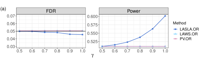
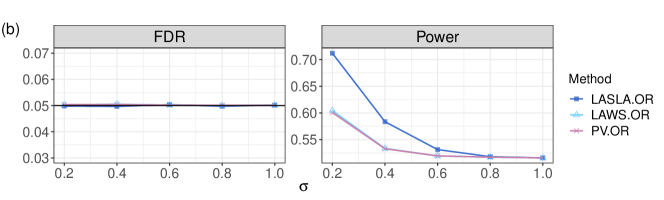
Figure 2.1: Empirical FDR and power comparison for oracle LASLA, LAWS and PV (unweighted p-value) with significance level $\alpha=0.05$. (a): Example 1; (b): Example 2.

2.6 The LASLA procedure

We now introduce the final step of LASLA: $p$-value thresholding. Let $\{w_{i}:i\in[m]\}$ be the data-driven LASLA weights. Recall that the weighted $p$-values are $\{P^{w}_{i}:i\in[m]\}$ with $P^{w}_{i}:=P_{i}/w_{i}$. Sort the weighted $p$-values from smallest to largest as $P^{w}_{(1)},\ldots,P^{w}_{(m)}$. To motivate the analysis, we assume that $P_{i}$ is independent with $w_{i}$, for $i\in[m]$. It follows that the expected number of false positives (EFP) in light of full network information $\mathcal{D}_{i},i\in[m]$ for a threshold $t^{w}$ can be calculated as:

$$\text{EFP}=\sum^{m}_{i=1}\mathbb{P}\{P^{w}_{i}\leq t^{w},\theta_{i}=0|\mathcal{D}_{i}\}=t^{w}\sum_{i=1}^{m}w_{i}\mathbb{P}(\theta_{i}=0|\mathcal{D}_{i})=t^{w}\sum_{i=1}^{m}w_{i}\left(1-\pi_{i}^{*}\right),$$ (2.11)

where the second equality follows from the standard assumption that $P_{i}$ is uniformly distributed given $\theta_{i}=0$ regardless of the side information. Suppose we reject $j$ hypotheses along the ranking provided by $P_{(i)}^{w}$ for $i\in[m]$, namely, set the threshold as $t^{w}=P^{w}_{(j)}$. Then the FDP can be estimated as: $\widehat{\text{FDP}}=\left(P^{w}_{(j)}/j\right)\sum_{i=1}^{m}w_{i}\left(1-\pi_{i}\right).$ We choose the largest possible threshold such that $\widehat{\text{FDP}}$ is less than the nominal level $\alpha$. Specifically, we find

$$k^{w}=\max\bigg{\{}j:\left(P^{w}_{(j)}/j\right)\sum_{i=1}^{m}w_{i}\left(1-\pi_{i}\right)\leq\alpha\bigg{\}},$$ (2.12)

and reject $H_{(1)},\cdots,H_{(k^{w})}$, which are the hypotheses with weighted $p$-values no larger than $P_{(k^{w})}^{w}$.

Remark 1.

We can substitute other thresholding rules for (2.12), such as the weighted BH (WBH) procedure [21]. However, numerical studies in Section S5 show that WBH can be overly conservative.

3 Theoretical Analysis

3.1 Asymptotic validity of the LASLA procedure

In this section we establish the asymptotic validity of LASLA when the $p$-values are marginally independent. The dependent cases will be studied in Section S7 of the Supplementary Material. We also show that LASLA is asymptotically more powerful than the BH procedure [20] under mild conditions. By convention, we assume that the auxiliary variables only affect the alternative distribution but not the null distribution of the primary statistics.

We start by analyzing the data-driven estimator $\pi_{i}$, as its consistency is needed for valid FDR control. The next assumption requires that the distributional quantities vary smoothly in the vicinity of location $i$.

1. For all $i,j$, $\mathbb{P}(P_{j}>\tau|\mathcal{D}_{j},D_{ij}=x)$ is continuous at $x$, and has bounded first and second derivatives.

It is important to note that marginally independent $p$-values will become dependent conditional on auxiliary data. The next assumption generalizes the commonly used “weak dependence” notion in [25]. It requires that most of the neighborhood $p$-values (conditional on auxiliary data) do not exhibit strong pairwise dependence.

1. $\text{Var}\left(\sum_{j\in\mathcal{N}_{i}}K_{h}(D_{ij}){\mathbb{I}}\{P_{j}>\tau\}|\boldsymbol{D}\right)\leq C\sum_{j\in\mathcal{N}_{i}}\text{Var}\left(K_{h}(D_{ij}){\mathbb{I}}\{P_{j}>\tau\}|\boldsymbol{D}_{j}\right)$ for some constant $C>1$, for all $i\in[m]$.

The next proposition establishes the convergence of $\pi_{i}$ to $\pi_{i}^{\tau}$.

Proposition 1.

Recall that $|\mathcal{N}_{i}|=m^{1-\epsilon}$. Under Assumptions (A1) and 2, if $m^{-1}\ll h\ll m^{-\epsilon}$, we have, uniformly for all $i\in[m]$, $\mathbb{E}\left[(\pi_{i}-\pi_{i}^{\tau})|\boldsymbol{D}_{i}\right]^{2}\rightarrow 0,\hskip 8.53581pt\text{as }\boldsymbol{D}_{i}\rightarrow\mathcal{D}_{i}.$

Define $Z_{i}=\Phi^{-1}(1-P_{i}/2)$ and denote by $\bm{Z}=(Z_{1},\ldots,Z_{m})^{\mathsf{\scriptscriptstyle T}}$ . We collect below several regularity conditions for proving the asymptotic validity of LASLA.

1. Assume that $\sum_{i=1}^{m}\mathbb{P}(\theta_{i}=0|\mathcal{D}_{i})\geq cm$ for some constant $c>0$ and that $\text{Var}\left[\sum_{i=1}^{m}I\{\theta_{i}=0\}|\mathcal{D}\right]=O(m^{1+\zeta})$ for some $0\leq\zeta<1$, where $\mathcal{D}=\{\mathcal{D}_{i}\}$.

2. Define $\mathcal{S}_{\rho}=\left\{i:1\leq i\leq m,|\mu_{i}|\geq(\log m)^{(1+\rho)/2}\right\},$ where $\mu_{i}=\mathbb{E}(Z_{i})$. For some $\rho>0$ and $\delta>0$, $|\mathcal{S}_{\rho}|\geq[{1}/({\pi}^{1/2}\alpha)+\delta]({\log m})^{1/2}$, where $\pi\approx 3.14$ is a constant.

Remark 2.

Condition 3 assumes that the model is sparse and that $\{\theta_{i}\}_{i=1}^{m}$ are not perfectly correlated (conditional on auxiliary data). Condition 4 requires that there are a slowly growing number of signals having magnitude of the order $\{(\log m)/n\}^{(1+\rho)/2}$ if $n$ samples are employed to obtain the $p$-value.

Let $t^{w}=P^{w}_{(k^{w})}$, where $k^{w}$ is calculated based on the step-wise algorithm (2.12) with weights from Algorithm 1. Denote by $\boldsymbol{\delta}^{w}\equiv\boldsymbol{\delta}^{w}(t^{w})=\{\delta_{i}^{w}(t^{w}):i\in[m]\}$ the set of decision rules, where $\delta_{i}^{w}(t^{w})={\mathbb{I}}\{P^{w}_{i}\leq t^{w}\}$. Then the FDP and FDR of LASLA are respectively given by

$$\text{FDP}(\boldsymbol{\delta}^{w})=\frac{\sum_{i=1}^{m}(1-\theta_{i}){\mathbb{I}}\{P_{i}^{w}\leq t^{w}\}}{\max\{\sum_{i=1}^{m}{\mathbb{I}}\{P_{i}^{w}\leq t^{w}\},1\}},\text{ and }{\text{FDR}}=\mathbb{E}\left\{\text{FDP}(\boldsymbol{\delta}^{w})\right\}.$$

The next theorem states that LASLA controls both the FDP and FDR at the nominal level asymptotically.

Theorem 1.

Assume that the $p$-values are marginally independent. Under the conditions in Proposition 1 and 3 and 4, $\mathop{\overline{\rm lim}}\limits_{\boldsymbol{D}_{i}\rightarrow\mathcal{D}_{i},\forall i}{\text{FDR}}\leq\alpha,\hskip 5.69054ptand\hskip 5.69054pt\lim\limits_{\boldsymbol{D}_{i}\rightarrow\mathcal{D}_{i},\forall i}\operatorname{\mathbb{P}}(\text{FDP}(\boldsymbol{\delta}^{w})\leq\alpha+\varepsilon)=1,$ for any $\varepsilon>0$.

3.2 Asymptotic power analysis

This section provides a theoretical analysis to demonstrate the benefit of the proposed weighting strategy. To simplify the analysis, we assume that the distance matrix $\mathcal{D}$ of the full network is known.

Denote by $\boldsymbol{\delta}^{v}(t)=\{\delta_{i}^{v}(t):i\in[m]\}$ a class of testing rules based on weighted $p$-values, where $\delta_{i}^{v}(t)={\mathbb{I}}\{P^{v}_{i}\leq t\}$, $P^{v}_{i}=P_{i}/v_{i}$ and $v_{i}$ is the weight that is independent of $P_{i}$. It can be shown that (e.g. Proposition 2 of [12]) under mild conditions, the FDR of $\boldsymbol{\delta}^{v}(t)$ can be written as $\text{FDR}\{\boldsymbol{\delta}^{v}(t)\}=Q^{v}(t|\mathcal{D})+o(1)$, where

$$Q^{v}(t|\mathcal{D})=\frac{\sum_{i=1}^{m}(1-\pi_{i}^{*})v_{i}t}{\sum_{i=1}^{m}(1-\pi_{i}^{*})v_{i}t+\sum_{i=1}^{m}\pi_{i}^{*}F_{1i}^{*}(v_{i}t|\mathcal{D}_{i})}$$

corresponds to the limiting value of the FDR, in which $\pi_{i}^{*}=\mathbb{P}(\theta_{i}=1|\mathcal{D}_{i})$. The power of $\boldsymbol{\delta}^{v}(t)$ can be evaluated using the expected number of true positives $\Psi^{v}(t)=\mathbb{E}\left\{\sum_{i=1}^{m}\delta_{i}^{v}(t)\theta_{i}\right\}=\sum_{i=1}^{m}\pi_{i}^{*}F_{1i}^{*}(v_{i}t).$

Let $\tilde{w}_{i}=w_{i}\sum_{j=1}^{m}(1-\pi_{j}^{*})/\sum_{j=1}^{m}\{(1-\pi_{j}^{*})w_{j}\}$, where $w_{i}$ are the oracle-assisted weights from Algorithm 1. It is easy to see that LASLA and $\boldsymbol{\delta}^{\tilde{w}}(t)$ share the same ranking of hypotheses. The goal is to compare the LASLA weights $(v_{i}=\tilde{w}_{i}:i\in[m])$ with the naive weights $\{v_{i}=1:i\in[m]\}$. Denote by $t_{o}^{v}=\sup\{t:Q^{v}(t)\leq\alpha\}$ the oracle threshold for the $p$-values with generic weights $\{v_{i}:i\in[m]\}$. The oracle procedure with LASLA weights and the (unweighted) oracle $p$-value procedure [24] are denoted by $\delta^{\tilde{w}}(t_{o}^{\tilde{w}})$ and $\delta^{1}(t_{o}^{1})$, respectively.

Next we discuss some assumptions needed in our power analysis. The first condition states that weights should be “informative” in the sense that $w_{i}$ are constructed in a way such that, on average, small/large $\pi_{i}^{*}$ correspond to small/large $w_{i}$. A similar assumption has been used in [21].

1. The oracle-assisted weights satisfy

   $$\frac{\sum_{i=1}^{m}(1-\pi_{i}^{*})}{\sum_{i=1}^{m}(1-\pi_{i}^{*})w_{i}}\cdot\frac{\sum_{i=1}^{m}\pi_{i}^{*}}{\sum_{i=1}^{m}\pi_{i}^{*}w_{i}^{-1}}\geq 1.$$

The second condition is concerned with the shape of the alternative $p$-value distributions. When the densities are homogeneous, i.e. $F_{1i}^{*}(t)\equiv F_{1}^{*}(t)$, it reduces to the condition that $x\rightarrow F_{1}^{*}(t/x)$ is a convex function, which is satisfied by commonly used density functions [26, 12].

1. $\sum_{i=1}^{m}a_{i}F_{1i}^{*}(t/x_{i})\geq\sum_{i=1}^{m}a_{i}F_{1i}^{*}({\sum_{j=1}^{m}a_{j}}t/{\sum_{j=1}^{m}a_{j}x_{j}})$ for any $0\leq a_{i}\leq 1$,
   $\min_{i\in[m]}\tilde{w}_{i}^{-1}\leq x_{i}\leq\max_{i\in[m]}\tilde{w}_{i}^{-1}$ and $t_{o}^{1}/\min_{i\in[m]}\tilde{w}_{i}^{-1}\leq 1$.

The above two conditions are mild in many practical settings. For example, we checked that both are easily fulfilled in all our simulation studies with the proposed LASLA weights. The next theorem provides insights on why the weighting strategy used in LASLA provides power gain, as we shall see in our numerical studies.

Theorem 2.

Assume that $p$-values are marginal independent and Conditions 5 and 6 hold. Then (a) $Q^{\tilde{w}}(t_{o}^{1})\leq Q^{1}(t_{o}^{1})\leq\alpha$; and (b) $\Psi^{\tilde{w}}(t_{o}^{\tilde{w}})\geq\Psi^{\tilde{w}}(t_{o}^{1})\geq\Psi^{1}(t_{o}^{1})$.

The theorem implies that (a) if the same threshold $t_{o}^{1}$ is used, then $\delta^{\tilde{w}}(t_{o}^{1})$ has smaller FDR and larger power than $\delta^{1}(t_{o}^{1})$; (b) the thresholds satisfy $t_{o}^{\tilde{w}}\geq t_{o}^{1}$. Since $\Psi^{v}(t)$ is non-decreasing in $t$, we conclude that $\delta^{\tilde{w}}(t_{o}^{\tilde{w}})$ (oracle procedure with LASLA weights) dominates $\delta^{\tilde{w}}(t_{o}^{1})$ and hence $\delta^{1}(t_{o}^{1})$ (unweighted oracle $p$-value procedure) in power.

4 Simulation

This section considers a model that mimics the network structure in the GWAS application of Section 5. The implementation details and additional simulation results for high-dimensional regression, latent variable model and multiple auxiliary samples are relegated to Section S5 of the Supplementary Material. Software implementing the algorithms and replicating all data experiments are available online at https://github.com/ZiyiLiang/r-lasla.

For $i\in[m]$, let $\theta_{i}\sim\text{Bernoulli}(0.1)$ denote the existence or absence of the signal at index $i$. The primary data $\boldsymbol{T}=(T_{i}:i\in[m])$ are generated as $T_{i}\sim(1-\theta_{i})N(0,1)+\theta_{i}N(\mu_{1},1)$ with $\mu_{1}$ controlling the signal strength. The distance matrix $\boldsymbol{D}=(D_{ij})_{1\leq i,j\leq m}$ follows $D_{ij}\sim I_{\{\theta_{i}=\theta_{j}\}}|N(\mu_{2},0.5)|+I_{\{\theta_{i}\neq\theta_{j}\}}|N(1,0.5)|,$ where $0\leq\mu_{2}\leq 1$ controls the informativeness of the distance matrix. Intuitively, if $\theta_{i}=\theta_{j}$, then $D_{ij}$ should be relatively small. We investigate two settings. Setting 1: Fix $\mu_{2}=0$, $m=1200$, vary $\mu_{1}$ from 2.5 to 3 by 0.1; Setting 2: Fix $\mu_{1}=3$, $m=1200$, vary $\mu_{2}$ from 0 to 1 by 0.2. $\boldsymbol{D}$ becomes less informative as $\mu_{2}$ gets closer to 1. The nominal level is set at $\alpha=0.05$.

Existing methods on structured multiple testing are not applicable due to the dimension mismatch of $\boldsymbol{T}$ and $\boldsymbol{D}$. Hence we only compare the data-driven LASLA (LASLA.DD) to the vanilla BH method that discards the auxiliary information. The simulation results, which are averaged over 100 randomized data sets, are summarized in Figure 4.1.

We can see that both methods control the FDR at the nominal level, and LASLA is conservative. In both settings, the power gain over BH is substantial. In Setting 2, we examine the performance of LASLA as the usefulness of $\boldsymbol{D}$ varies. The power gap between two methods becomes smaller as $\mu_{2}$ approaches 1. Note that even if $\boldsymbol{D}$ becomes completely non-informative ($\mu_{2}=1$), LASLA still outperforms BH. This is due to the fact that LASLA captures the asymmetry within the alternative distribution of the primary statistics. This is consistent with the finding in [16] that the lfdr ([27]) procedure dominates BH in power.

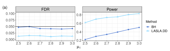
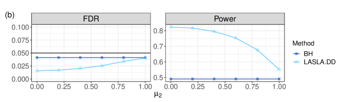
Figure 4.1: Empirical FDR and power comparison for data-driven LASLA and BH. (a): Setting 1; (b): Setting 2.

5 Detecting T2D-associated SNPs with auxiliary data from linkage analysis

This section focuses on conducting association studies of Type 2 diabetes (T2D), a prevalent metabolic disease with strong genetic links. Our primary goal is to identify SNPs associated with T2D in diverse populations. We construct distance matrix from LD information to gain valuable insights into the genetic basis of complex diseases as previously described in Section 2.1.

[28] performs a meta-analysis to combine 23 studies on a total of 77,418 individuals with T2D and 356,122 controls. For illustration purpose, we randomly choose $m=5000$ SNPs from Chromosome 6 to be the target of inference. Primary statistics are the $z$-values provided in [28] and the auxiliary LD matrix is constructed by the genetic analysis tool Plink from the 1000 Genomes (1000G) Phase 3 Database. It is important to note that the primary and auxiliary data are collected from different populations and are not matched in dimension.

Table 1: Number of rejections by different methods

FDR	0.001	0.01	0.05	0.1
BH	35	61	128	179
LASLA	36	101	184	271

Table 2: Number of rejections by Bonferroni Correction

FWER	0.001	0.01	0.05	0.1
Bonferroni	21	29	35	43

We apply BH and LASLA at different FDR levels and compare them with the Bonferroni correction which is commonly used in GWAS to control Family-wise Error Rate (FWER). The number of rejections by different methods are summarized in Tables 1 and 2. Both BH and LASLA are more powerful than the Bonferroni method. Moreover, at the same FDR level, LASLA makes notably more rejections than BH, and the discrepancy becomes even larger as the nominal FDR level increases.

To illustrate the power gain of LASLA over BH, we visualize the rejected hypotheses in Figure 5.1. Red nodes in the figure present SNPs detected by LASLA but not by BH at FDR level 0.05. Nodes connected by an edge are in linkage disequilibrium. The graph highlights LASLA’s ability to leverage the LD matrix’s network structure for inference, leading to the identification of clusters of SNPs in LD. In contrast, BH could potentially miss important variants. Notably, LASLA detects T2D-risk variants within the gene CCHCR1, a new candidate gene for T2D reported in a recent study by [29].

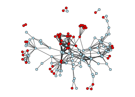
Figure 5.1: Sub-network identified by LASLA (all nodes). BH only detects the blue nodes.

6 Acknowledgements

The research of Yin Xia was supported in part by the National Natural Science Foundation of China (Grant No. 12022103). The research of Tony Cai was supported in part by the National Science Foundation (Grant DMS-2015259) and National Institutes of Health (Grant R01-GM129781).

7 Supplementary Material

The Supplementary material includes additional simulations and applications of LASLA, as well as the discussion to dependent primary statistics and the proofs of all theoretical results.

Supplementary Material for “Locally Adaptive Algorithms for Multiple Testing with Network Structure, with Application to Genome-Wide Association Studies”

In this supplement, we discuss additional applications of LASLA in Supplement S1; the construction of corresponding distance matrices in Supplement S2; implementation details and additional simulation results in Supplement S5. Related background reviews on the sparsity-adaptive weights and an alternative weight construction are presented in Supplements S3 and S4. Proofs of the main results are collected in Supplement S6. Finally, Supplements S7 and S8 extend the discussion to dependent primary statistics.

Appendix S1 Additional applications

LASLA has a wide range of applications aside from the network-structured data like the GWAS example discussed in the main article. In this section, we introduce two additional challenging settings: data-sharing regression and integrative inference with multiple auxiliary data sets. In both scenarios, traditional frameworks are not applicable since the auxiliary data $\boldsymbol{U}$ and the primary data $\boldsymbol{T}$ do not match in dimension.

Example 1. Data-sharing high-dimensional regression. Suppose we are interested in identifying genetic variants associated with type II diabetes (T2D). Consider a high-dimensional regression model:

$$\boldsymbol{Y}=\boldsymbol{\mu}+\boldsymbol{X}\boldsymbol{\beta}+\boldsymbol{\epsilon},$$ (S1)

where $\boldsymbol{Y}=(Y_{1},\ldots,Y_{n})^{{\mathsf{\scriptscriptstyle T}}}$ are measurements of phenotypes, $\boldsymbol{\mu}=\mu\boldsymbol{1}^{{\mathsf{\scriptscriptstyle T}}}$ is the intercept, with $\boldsymbol{1}^{{\mathsf{\scriptscriptstyle T}}}$ being a vector of ones, $\boldsymbol{\beta}=(\beta_{1},\dots,\beta_{m})^{{\mathsf{\scriptscriptstyle T}}}$ is the vector of regression coefficients, $\bm{X}\in\mathbb{R}^{n\times m}$ is the matrix of measurements of genomic markers, and $\bm{\epsilon}=(\epsilon_{1},\dots,\epsilon_{n})^{\mathsf{\scriptscriptstyle T}}$ are random errors.

Both genomics and epidemiological studies have provided evidence that complex diseases may have shared genetic contributions. The power for identifying T2D associated genes can be enhanced by incorporating data from studies of related diseases such as cardiovascular disease (CVD) and ischaemic stroke. Consider models for other studies:

$${\boldsymbol{Y}}^{k}={\boldsymbol{\mu}}^{k}+{\boldsymbol{X}}^{k}{\boldsymbol{\beta}}^{k}+{\boldsymbol{\epsilon}}^{k},$$ (S2)

where the superscript $k$ indicates that the auxiliary data are collected from disease type $k\in[K]$. The notations ${\boldsymbol{Y}}^{k}$, $\boldsymbol{\mu}^{k}$, $\boldsymbol{\bm{\beta}}^{k}$, $\bm{X}^{k}$ and $\bm{\epsilon}^{k}$ have similar explanations as above. The identification of genetic variants associated with T2D can be formulated as a multiple testing problem (2.1), where $\boldsymbol{\theta}=(\theta_{i}:i\in[m])=\{{\mathbb{I}}(\beta_{i}\neq 0):i\in[m]\}$ is the primary parameter of interest. The primary and auxiliary data sets are $\boldsymbol{T}=(\bm{Y},\bm{X})$ and $\boldsymbol{U}=\{(\bm{Y}^{k},\bm{X}^{k}):k\in[K]\}$, respectively. The auxiliary data $\boldsymbol{U}$ can provide useful guidance by prioritizing the shared risk factors and genetic variants.

Example 2. Integrative “omics” analysis with multiple auxiliary data sets. The rapidly growing field of integrative genomics calls for new frameworks for combining various data types to identify novel patterns and gain new insights. Related examples include (a) the analysis of multiple genomic platform (MGP) data, which consist of several data types, such as DNA copy number, gene expression and DNA methylation, in the same set of specimen ([30]); (b) the integrated copy number variation (iCNV) caller that aims to boost statistical accuracy by integrating data from multiple platforms such as whole exome sequencing (WES), whole genome sequencing (WGS) and SNP arrays ([31]); (c) the integrative analysis of transcriptomics, proteomics and genomic data ([32]). The identification of significant genetic factors can be formulated as (2.1) with mixed types of auxiliary data.

Appendix S2 Forming local neighborhoods: illustrations

Recall that, in Section 1, LASLA first summarize the structural knowledge in a distance matrix $\boldsymbol{D}\in\mathbb{R}^{m\times m}$ where $m$ is the number of hypotheses. The distance matrix describes the relation between each pair of hypotheses in the light of the auxiliary data. For the GWAS example detailed in Section 1, $\boldsymbol{D}=(1-r^{2}_{ij}:i,j\in[m])$ where $r_{ij}$ measures the linkage disequilibrium between the two SNPs $i\text{ and }j$.

In Example 1 (data-sharing regression) from Supplement S1, we can extract the structural knowledge provided by the related regression problems via Mahalanobis distance [33]. Specifically, let $\{\hat{\boldsymbol{\beta}}^{k}=(\hat{\beta}^{k}_{1},\dots,\hat{\beta}^{k}_{m})^{{\mathsf{\scriptscriptstyle T}}}:k\in[K]\}$ denote the estimation of $\{\boldsymbol{\beta}^{k}=(\beta^{k}_{1},\dots,\beta^{k}_{m})^{{\mathsf{\scriptscriptstyle T}}}:k\in[K]\}$. Denote by $\hat{\boldsymbol{\beta}_{i}}=(\hat{\beta}^{k}_{i}:k\in[K])$ the vector of estimated coefficients for the $i$th genomic marker across $K$ different studies. The distance matrix $\boldsymbol{D}=(D_{ij})_{i,j\in[m]}$ is then constructed via Mahalanobis distance with $D_{ij}=({\hat{\boldsymbol{\beta}}_{i}}-{\hat{\boldsymbol{\beta}}_{j}}){\hat{\Sigma}}_{\boldsymbol{\beta}}^{-1}({\hat{\boldsymbol{\beta}}_{i}}-{\hat{\boldsymbol{\beta}}_{j}})^{{\mathsf{\scriptscriptstyle T}}}$ , where ${\hat{\Sigma}}_{\boldsymbol{\beta}}$ is the estimated covariance matrix based on $\{\hat{\boldsymbol{\beta}}_{i}:i\in[m]\}$. Similarly, in Example 2 (analysis with multiple auxiliary data sets), suppose we collect a multivariate variable $\boldsymbol{U}_{i}$ from different platforms as the side information for gene $i$, then the Mahalanobis distance can be used to construct a distance matrix $\boldsymbol{D}=(D_{ij})_{i,j\in[m]}$ with $D_{ij}=({\boldsymbol{U}_{i}}-{\boldsymbol{U}_{j}}){\hat{\Sigma}}_{U}^{-1}({\boldsymbol{U}_{i}}-{\boldsymbol{U}_{j}})^{{\mathsf{\scriptscriptstyle T}}}$, where $\hat{\Sigma}_{U}$ is the estimated covariance matrix based on the auxiliary sample $\{\boldsymbol{U}_{i}:i\in[m]\}$.

We emphasize that LASLA is not limited to the aforementioned examples. Most of the traditional covariate-assisted methods focus on the array-like auxiliary data $\boldsymbol{U}=\{U_{i}:i=1,2,\ldots\}$ that matches primary data coordinate by coordinate. LASLA can also handle this dimension-matching side information as the latter can be represented by a distance matrix $\boldsymbol{D}$ through simple manipulations. Below, we provide a list of practical types of side information and their corresponding methods for constructing the distance matrix.

• A vector of categorical covariates. The elements in $\boldsymbol{U}$ take discrete values and the local neighborhoods can be defined as groups. With suitably chosen weights LASLA reduces to the methods considered in [26], [4] and [9] that are developed for multiple testing with groups.

• A vector of continuous covariates. We can define distance as either the absolute difference or the standardized difference in rank $D_{ij}=|\hat{F}_{m}(U_{i})-\hat{F}_{m}(U_{j})|$, where $\hat{F}_{m}(t)$ is the empirical CDF.

• Spatial locations. Such structures have been considered in, for example, [2], [14] and [12]. The locations are viewed as covariates and $D_{ij}$ is the Euclidean distance between locations $i$ and $j$.

• The correlations in a network or partial correlations in graphical models. See the GWAS example discussed in Section 1 of the main article.

• Multiple auxiliary samples. The Mahalanobis distance or its generalizations [33] can be used to calculate the distance matrix $\boldsymbol{D}$.

Note that in practical applications, it could be beneficial to “standardize” the distance matrix $\boldsymbol{D}$; this step ensures algorithm robustness. A more comprehensive discussion on the implementation details is relegated to Supplement S5.1.

Appendix S3 Details on sparsity-adaptive weights

Recall the definition from Section 2.2 that the primary statistics $T_{i}$ has the hypothetical mixture distribution:

$$F^{*}_{i}(t)=(1-\pi_{i}^{*})F_{0}(t)+\pi_{i}^{*}F^{*}_{1i}(t)$$

for $i\in[m]$. The quantity $\pi_{i}^{*}$ indicates the sparsity level of signals at location $i$, and $\pi_{i}^{*}$ is allowed to be heterogeneous across $m$ testing locations.

The key idea in existing weighted FDR procedures such as GBH [26], SABHA ([4]) and LAWS ([12]) is to construct weights that leverage $\pi_{i}^{*}$ by prioritizing the rejection of the null hypotheses in groups or at locations where signals appear to be more frequent. Specifically, SABHA defines the weight as $w^{\text{sabha}}_{i}=1/(1-\pi_{i}^{*})$, and LAWS as $w^{\text{laws}}_{i}=\pi_{i}^{*}/(1-\pi_{i}^{*})$. The sparsity adaptive-weights have an intuitive interpretation. Consider the LAWS weight $w^{\text{laws}}_{i}$, if $\pi_{i}^{*}$ is large, indicating a higher occurrence of signals at location $i$, the weighted $p$-value $P^{w}_{i}:=P_{i}/w^{\text{laws}}_{i}=(1-\pi_{i}^{*})P_{i}/\pi_{i}^{*}$ will be smaller, up-weighting the significance level of hypothesis $i$. However, compared to the proposed weights, such weighting scheme ignores structural information in alternative distributions as discussed in Section 2.5.

Appendix S4 Alternative weight construction

Recall that $\mathcal{N}_{i}=\{j\neq i:D_{ij}\leq a_{\epsilon}\}$ is the neighborhood index set which only contains indexes with distance to $i$ smaller than $a_{\epsilon}$ and satisfies $|\mathcal{N}_{i}|=m^{1-\epsilon}$ for some small constant $\epsilon>0$. Additionally, $D_{ij_{1}}\leq D_{ij_{2}}$ for any $j_{1}\in\mathcal{N}_{i}$, $j_{2}\notin\mathcal{N}_{i}$, and $j_{2}\neq i$. The alternative computationally efficient procedure mentioned in Section 2.4 is summarized in Algorithm S2 below.

Algorithm S2 Simplified Oracle-assisted weights

1:  Input: the nominal FDR level $\alpha$, $\epsilon$ specifying the size of the sub-neighborhood, kernel function $K(\cdot)$, primary statistics $\boldsymbol{T}=\{T_{i}:i\in[m]\}$ and distance matrix $\boldsymbol{D}=(D_{ij}:i,j\in[m])$.

2:  For $i\in[m]$ do:

3:    Estimate $\pi_{i}$ as given by (2.5) with summation taken over $\mathcal{N}_{i}$.

4:    Estimate $f_{i}(t)$ as given by (2.6) with summation taken over $\mathcal{N}_{i}$.

5:    Compute $L_{i}$ as given by (2.7). Denote the sorted statistics by $L_{(1)}\leq\ldots\leq L_{(m)}$.

6:  Choose $L_{(k)}$ to be the oracle threshold, where $k=\max\{j\in[m]:j^{-1}\sum^{j}_{i=1}{L_{(i)}\leq\alpha}\}$.

7:  For $i\in[m]$ do:

8:    If $T_{i}\geq 0$ then: Compute $t^{+}_{i}$ as given by (2.9), and the weight by $w_{i}=1-F_{0}(t^{+}_{i})$.

9:    If $T_{i}<0$ then: Compute $t^{-}_{i}$ as given by (2.10), and the weight by $w_{i}=F_{0}(t^{-}_{i})$.

10:  Output: Oracle-assisted weights $\{w_{i}:i\in[m]\}$.

Appendix S5 Implementation Details and Additional Numerical Results

In this section, we provide the numerical implementation details and collect additional simulation results for data-sharing high-dimensional regression, latent variable model and multiple auxiliary samples.

S5.1 Implementation Details

In all of our numerical results, the bandwidth $h$ for the kernel estimations in (2.5) and (2.6) is chosen automatically by applying the density function with the option “SJ-ste” in R package stats. For the size of neighborhoods $m^{1-\epsilon}$, the default choice for $\epsilon$ is 0.1 for marginally independent $p$-values, while for dependent $p$-values, we set $\epsilon=0$ to comply with our FDR control theory under weak dependence in Supplement S7.

To enhance algorithmic robustness and numerical performance, we perform a data-driven scaling of the distance matrix $\boldsymbol{D}$ by a constant factor $a$. A practical guideline is to ensure that the spread of entries in the scaled distance matrix $\boldsymbol{D}/a$ is similar to that of the entries in $\boldsymbol{T}$. One can use the interquartile range (IQR) to measure the data spread. Below are the adjustments made for each numerical experiment in order of appearance: (1) $a=1/2$ for the network example in Section 4; (2) $a=1.4$ for the GWAS application in Section 5; (3) $a=4$ for the high-dimensional regression models in Supplement S5.2; (4) $a=1$ for the latent variable settings in Supplement S5.3; (5) $a=5$ for the multiple auxiliary experiments in Supplement S5.4.

S5.2 Data-sharing high-dimensional regression

Example 2 in Supplement S1 discussed how the knowledge in regression models from related studies can be transferred to improve the inference on regression coefficients from the primary model. This section designs simulation studies to illustrate the point.

Consider the regression model (S1) defined in Supplement S1 with $\bm{X}_{ij}\sim N(0,1)$ for $i\in[n],j\in[m]$ where $\bm{X}_{ij}$ denotes the entry of $\bm{X}$ at coordinate $(i,j)$; $\epsilon_{i}\sim N(0,1)$ for $i\in[n]$. Let $\operatorname{\mathbb{P}}(\beta_{i}=0)=0.9$. For the non-null locations, $\beta_{i}\sim(-1)^{u}|N(\mu,0.1)|$; $u\sim\text{Bernoulli}(0.2)$. Note that signals will be more likely to take positive signs, hence asymmetric rejection rules are desired.

Models from $K$ related studies are generated by model (S2). If the auxiliary model is closely related to the primary model, they tend to share similar coefficients, therefore we generate the coefficients for study $k\in[K]$ as ${\boldsymbol{\beta}}^{k}=\boldsymbol{\beta}+\boldsymbol{\sigma},$ where each coordinate of $\boldsymbol{\sigma}$ is drawn from normal distribution $N(0,\sigma)$. Other quantities are defined similarly as the primary model.

We compute the distance matrix $\boldsymbol{D}$ using the Mahalanobis distance on the estimated coefficients as specified in Supplement S2. Fix $K=3,n=1000,m=800$, consider the following settings:

• Setting 1: Fix $\mu=0.3$, vary the noise level $\sigma$ from 0.05 to 0.1 by 0.01.

• Setting 2: Fix $\sigma=0.05$, vary the signal strength $\mu$ from 0.25 to 0.35 by 0.025.

We compare BH with the data-driven LASLA. To apply LASLA, it’s essential to have knowledge of the null distribution for the test statistics. In this simulation we use the ordinary least square estimators and $T_{i}$ follows a $t$-distribution. Alternatively, one can explore the approach outlined in [9], where the test statistics follow the $N(0,1)$ distribution asymptotically. Figure S1 shows that LASLA can effectively leverage the side information from related studies.

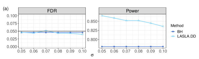
Figure S1: Empirical FDR and power comparison. (a): Regression Setting 1; (b): Regression Setting 2.

S5.3 Latent variable setting

Suppose the primary and auxiliary data are associated with a common latent variable $\bm{\xi}=(\xi_{i}:i\in[m])$ where $\xi_{i}\sim(1-\theta_{i})\Delta_{0}+\theta_{i}N(\mu,1)$ and $\Delta_{0}$ is the Dirac delta function, namely, $\xi_{i}=0$ if $\theta_{i}=0$. The primary data $\boldsymbol{T}=(T_{i}:i\in[m])$ and auxiliary data $\boldsymbol{U}=(U_{i}:i\in[m])$ respectively follow:

$$T_{i}\sim N(\xi_{i},1),\quad U_{i}\sim N(\xi_{i},\sigma_{s}^{2}),$$ (S1)

where $\sigma_{s}$ controls the informativeness the auxiliary data. Our goal is to test $m$ hypotheses on $\theta_{i}$ as stated in (2.1). Fix $m=1200$ and let $\theta_{i}\sim\text{Bernoulli}(0.1)$, independently for $i\in[m]$. We consider two settings:

• Setting 1: Fix $\mu=2.5$, vary $\sigma_{s}$ from 0.5 to 2 by 0.25.

• Setting 2: Fix $\sigma_{s}=1$ , vary $\mu$ from 3 to 4 by 0.2.

We compute the distance matrix $\boldsymbol{D}$ from the auxiliary data $\boldsymbol{U}$ using the Euclidean distance, i.e. $D_{ij}=|U_{i}-U_{j}|$. The following methods are implemented:

• Benjamini-Hochberg procedure (BH);

• LASLA with known $\pi_{i}^{*}$ and $f_{i}^{*}(t)$ (LASLA.OR);

• Data-driven LASLA (LASLA.DD);

• Data-driven SABHA (SABHA.DD) as reviewed in Supplement S3;

• WBH method with LASLA weights (WBH) discussed in Section 2.6, Remark 1.

The result is summarized in Figure S2. In both settings, LASLA has smaller FDR than SABHA but still dominate SABHA in power due to the fact that SABHA is entirely $p$-value based and its weights only takes sparsity into account. Some other $p$-value based methods like AdaPT [14] may also suffer from power loss since the potential asymmetry in the primary statistics is ignored.

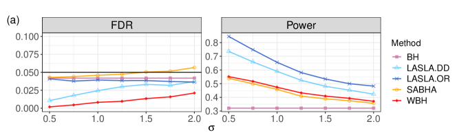
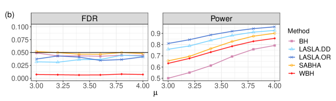
Figure S2: Empirical FDR and power comparison. (a): Latent variable Setting 1; (b): Latent variable Setting 2.

S5.4 Multiple auxiliary samples

We explore two scenarios with multiple auxiliary samples: (1) all samples are informative; (2) some samples are non-informative. Similar to the previous section, consider a latent variable $\bm{\xi}=(\xi_{i}:i\in[m])$ where $\xi_{i}\sim(1-\theta_{i})\Delta_{0}+\theta_{i}N(\mu,1)$ and $\theta_{i}\sim\text{Bernoulli}(0.1)$. The primary statistics $T_{i}\sim N(\xi_{i},1)$ for $i\in[m]$. The goal is to make inference on the unknown $\theta_{i}$. Let $\boldsymbol{U}^{k}=(U^{k}_{i}:i\in[m])$ denote the $k$th auxiliary sequence for $k\in[K]$. If $\boldsymbol{U}$ is informative, it should carry knowledge on the underlying signal $\theta_{i}$. Hence we introduce the first setting where all auxiliary samples are associated with the latent variable $\bm{\xi}$:

• Setting 1: $U^{k}_{i}\sim N(\xi_{i},\sigma^{2}_{s})$ for $i\in[m],k=1,...,4$.

Let $\gamma_{i}\sim\text{Bernoulli}(0.1)$ for $i\in[m]$ independently of everything else, and $\psi_{i}\sim(1-\gamma_{i})\Delta_{0}+\gamma_{i}N(\mu,1)$. Consider:

• Setting 2: $U^{k}_{i}\sim N(\xi_{i},\sigma^{2}_{s})$ , for $k=1,2$; $U^{k}_{i}\sim N(\psi_{i},\sigma^{2}_{s})$ , for $k=3,4$.

Note that $\gamma_{i}$ being independent of $\theta_{i}$ can lead to significant divergence between the latent variables $\psi_{i}$ and $\xi_{i}$, potentially making $\boldsymbol{U}^{3}$ and $\boldsymbol{U}^{4}$ anti-informative. The construction of $\boldsymbol{D}$ from $\{\boldsymbol{U}^{k}\}_{k\in[K]}$ is not unique, we explore two different methods: using Mahalanobis distance vs using Euclidean distance with the averaged data $U^{\text{avg}}_{i}=\frac{1}{4}(U_{i}^{1}+U_{i}^{2}+U_{i}^{3}+U_{i}^{4})$ for $i\in[m]$. We assess their effectiveness under varying degrees of informativeness exhibited by the auxiliary samples.

In both settings, we fix $m=1200,\mu=3$, and change $\sigma_{s}$ from 0.5 to 2 by 0.25. The results are summarized in Figure S3. Intuitively, the averaging method reduces variance when all auxiliary samples are informative and leads to power gain over the Mahalanobis approach. However, the latter appears to be more robust when some samples are anti-informative.

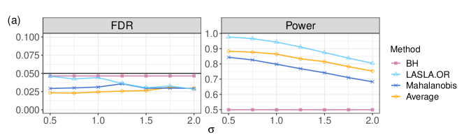
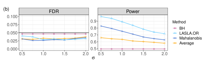
Figure S3: Empirical FDR and power comparison. (a): Multiple auxiliary samples Setting 1; (b): Multiple auxiliary samples Setting 2.

Appendix S6 Proof of Main Results

Recall that $\boldsymbol{D}_{i}$ be the $i$th column of $\boldsymbol{D}$, and $\mathcal{D}_{i}$ is a continuous finite domain (w.r.t. coordinate $i$) in $\mathbb{R}$ with positive measure by adapting the fixed-domain asymptotics in [23]. Each $d\in\mathcal{D}_{i}$ is a distance and $0\in\mathcal{D}_{i}$. The two sets $\boldsymbol{D}_{i}$ and $\mathcal{D}_{i}$ can be viewed as distances measured from a partial/full network, respectively, and $\boldsymbol{D}_{i}\subset\mathcal{D}_{i}$.

Throughout the proofs, we assume that $\boldsymbol{D}_{i}\rightarrow\mathcal{D}_{i}$ as $m\rightarrow\infty$ in the sense that, for any $d_{0}\in\mathcal{D}_{i}$, there exists at least an index $j$ such that $|D_{ij}-d_{0}|=O(m^{-1})$ as $m\rightarrow\infty$.

S6.1 Proof of Proposition 1

Proof.

For simplicity of notation, throughout we omit the conditioning on $\mathcal{D}$, and use $\mathbb{P}(P_{j}>\tau|D_{ij}=x)$ and $\mathbb{P}(P_{i}>\tau)$ to denote $\mathbb{P}(P_{j}>\tau\mid\mathcal{D}_{j},D_{ij}=x)$ and $\mathbb{P}(P_{i}>\tau\mid\mathcal{D}_{i})$ respectively. Recall that

$$1-\pi_{i} =\frac{\sum_{j\in\mathcal{N}_{i}}[{K_{h}(D_{ij}){\mathbb{I}}\{P_{j}>\tau\}}]}{(1-\tau)\sum_{j\in\mathcal{N}_{i}}{K_{h}(D_{ij})}}$$

Also note that, for all $i\in[m]$,

$$\operatorname{\mathbb{E}}\bigg{(}\sum_{j\in\mathcal{N}_{i}}[{K_{h}(D_{ij}){\mathbb{I}}\{{P_{j}>\tau}\}}\mid\boldsymbol{D}\bigg{)}=\sum_{j\in\mathcal{N}_{i}}[{K_{h}(D_{ij})\operatorname{\mathbb{P}}(P_{j}>\tau\mid\boldsymbol{D}_{j})}]$$

Then by $m^{-1}\ll h\ll m^{-\epsilon}$, as $\boldsymbol{D}_{i}\rightarrow\mathcal{D}_{i}$, we have

$$\frac{\operatorname{\mathbb{E}}(1-\pi_{i}\mid\boldsymbol{D})}{{\int_{\tilde{\mathcal{D}}_{i}}{K_{h}(x)\operatorname{\mathbb{P}}(P_{j_{x}}>\tau\mid D_{ij_{x}}=x)}\,dx}/{(1-\tau)\int_{\tilde{\mathcal{D}}_{i}}{K_{h}(x)}\,dx}}\rightarrow 1,$$

where $j_{x}$ represents the index such that $D_{ij_{x}}=x$ and $\tilde{\mathcal{D}}_{i}$ is the limit of $\{D_{ij},j\in\mathcal{N}_{i}\}$ in the asymptotic framework described in Section 2.3. Using Taylor expansion at $x=0$, combined with Assumption (A1), we have

$$\int_{\tilde{\mathcal{D}}_{i}}{K_{h}(x)\operatorname{\mathbb{P}}(P_{j_{x}}>\tau\mid D_{ij_{x}}=x)}\,dx$$

$$=\operatorname{\mathbb{P}}(P_{i}>\tau)\int_{\tilde{\mathcal{D}}_{i}}K_{h}(x)\,dx+\mathbb{P}^{\prime}(P_{i}>\tau)\int_{\tilde{\mathcal{D}}_{i}}xK_{h}(x)\,dx$$

$$+\frac{\mathbb{P}^{\prime\prime}(P_{i}>\tau)}{2}\int_{\tilde{\mathcal{D}}_{i}}x^{2}K_{h}(x)\,dx+\textit{O}(h^{2}).$$

Thus, by the assumptions of $K(\cdot)$ in (2.4), uniformly for all index $i$, there exists some constant $c>0$ such that

$$\left[\operatorname{\mathbb{E}}(\pi_{i}\mid\boldsymbol{D})-\pi_{i}^{\tau}\right]^{2}$$

$$\leq\bigg{(}c\int_{\tilde{\mathcal{D}}_{i}}xK_{h}(x)\,dx\bigg{/}\int_{\tilde{\mathcal{D}}_{i}}K_{h}(x)\,dx+c\int_{\tilde{\mathcal{D}}_{i}}x^{2}K_{h}(x)\bigg{/}\int_{\tilde{\mathcal{D}}_{i}}K_{h}(x)\,dx\bigg{)}^{2}+o(1)$$

$$\rightarrow 0,\hskip 28.45274pt\text{as }h\rightarrow 0.$$

Now we inspect the variance term. By Condition 2, there exists a constant $c^{\prime}>1$,

$$\operatorname{Var}\bigg{(}\sum_{j\in\mathcal{N}_{i}}[K_{h}(D_{ij}){\mathbb{I}}\{P_{j}>\tau\}]\mid\boldsymbol{D}\bigg{)}$$

$$\leq c^{\prime}\sum_{j\in\mathcal{N}_{i}}[{K^{2}_{h}(D_{ij})\operatorname{Var}\big{(}{\mathbb{I}}\{P_{j}>\tau\}\mid\boldsymbol{D}_{j}\big{)}}]$$

$$=c^{\prime}\sum_{j\in\mathcal{N}_{i}}\left[{K^{2}_{h}(D_{ij})\operatorname{\mathbb{P}}(P_{j}>\tau\mid\boldsymbol{D}_{j})\left\{1-\operatorname{\mathbb{P}}(P_{j}>\tau\mid\boldsymbol{D}_{j})\right\}}\right].$$

Hence, as $h\gg m^{-1}$, by the assumptions of $K(\cdot)$ in (2.4) and that it is positive and bounded, we have

$$\operatorname{Var}(1-\pi_{i}) \leq c^{\prime\prime}m^{-1}\frac{\int_{\tilde{\mathcal{D}}_{i}}K^{2}_{h}(x)\,dx}{[(1-\tau)\int_{\tilde{\mathcal{D}}_{i}}K_{h}(x)\,dx]^{2}}$$

$$\leq c^{\prime\prime}(mh)^{-1}\frac{\int_{\mathbb{R}}K^{2}(y)\,dy}{[(1-\tau)\int_{\tilde{\mathcal{D}}_{i}}K_{h}(x)\,dx]^{2}}$$

$$\leq c^{\prime\prime\prime}(mh)^{-1}=o(1),$$

for some constant $c^{\prime\prime},c^{\prime\prime\prime}>0$. Hence, as $\boldsymbol{D}_{i}\rightarrow\mathcal{D}_{i}$, by combining the bias term and variance term, the consistency result is proved. ∎

S6.2 Proof of Theorem 1

Proof.

For simplicity of notation, throughout we omit the conditioning on $\mathcal{D}$, and use $\mathbb{P}(\theta_{i}=0)$ to denote $\mathbb{P}(\theta_{i}=0\mid\mathcal{D}_{i})$. Note that, by Algorithm S2, the FDP of LASLA at the thresholding level $t$ can be calculated by

$$FDP(t) =\frac{\sum_{i=1}^{m}{\mathbb{I}}\{P_{i}^{w}\leq t,\theta_{i}=0\}}{\max[\sum_{i=1}^{m}{\mathbb{I}}\{P_{i}^{w}\leq t\},1]}$$

$$=\frac{\sum_{i=1}^{m}\mathbb{P}(P_{i}^{w}\leq t,\theta_{i}=0\mid w_{i},\mathcal{D}_{i})}{\max[\sum_{i=1}^{m}{\mathbb{I}}\{P_{i}^{w}\leq t\},1]}\cdot\frac{\sum_{i=1}^{m}{\mathbb{I}}\{P_{i}^{w}\leq t,\theta_{i}=0\}}{\sum_{i=1}^{m}\mathbb{P}(P_{i}^{w}\leq t,\theta_{i}=0\mid w_{i},\mathcal{D}_{i})},$$

where for the ease of notation, throughout we use $\mathbb{P}(P_{i}^{w}\leq t,\theta_{i}=0)$ to denote $\mathbb{P}(P_{i}^{w}\leq t,\theta_{i}=0\mid w_{i},\mathcal{D}_{i})$, and use $\mathbb{P}(P_{i}^{w}\leq t\mid\theta_{i}=0)$ to denote $\mathbb{P}(P_{i}^{w}\leq t\mid\theta_{i}=0,w_{i})$, and similarly for the corresponding $z$-values.

Step 1: We first show that, uniformly for all $i\in[m]$, we have

$$\sum_{i=1}^{m}\mathbb{P}(P_{i}^{w}\leq t,\theta_{i}=0)\leq{(1+o_{\mathbb{P}}(1))\sum_{i=1}^{m}w_{i}(1-\pi_{i})t.}$$ (S1)

Note that, in Algorithm 1, $T_{i}$ is not used in the computation of $w_{i}$. Then by the assumption that all $p$-values are marginally independent, $T_{i}$ is independent of $w_{i}$. Hence, we have

$$\sum_{i=1}^{m}\mathbb{P}(P_{i}^{w}\leq t,\theta_{i}=0) =\sum_{i=1}^{m}\mathbb{P}(P_{i}^{w}\leq t\mid\theta_{i}=0)\mathbb{P}(\theta_{i}=0)$$

$$=\sum_{i=1}^{m}w_{i}(1-\pi_{i}^{*})t\leq\sum_{i=1}^{m}w_{i}(1-\pi_{i}^{\tau})t,$$

where the last inequality follows from the fact that $\pi_{i}^{\tau}$ is a conservative approximation of $\pi_{i}^{*}$ as showed in [12]. By the result of Proposition 1 and Assumption 3, together with the fact that $\xi\leq w_{i}\leq 1$ for $i\in[m]$, we have

$$\sum_{i=1}^{m}\mathbb{P}(P_{i}^{w}\leq t,\theta_{i}=0)\leq\sum_{i=1}^{m}w_{i}(1-\pi_{i}+o_{\mathbb{P}}(1))t={(1+o_{\mathbb{P}}(1))\sum_{i=1}^{m}w_{i}(1-\pi_{i})t.}$$

Hence (S1) is proved.

Step 2: We next show that

$$\Bigg{|}\frac{\sum_{\theta_{i}=0}\mathbb{P}(P_{i}^{w}\leq t\mid\theta_{i}=0)-\sum_{i=1}^{m}\mathbb{P}(P_{i}^{w}\leq t,\theta_{i}=0)}{\sum_{i=1}^{m}\mathbb{P}(P_{i}^{w}\leq t,\theta_{i}=0)}\Bigg{|}\rightarrow 0,$$ (S2)

in probability. Define the event

$$B=\left[\{\theta_{i}\}_{i=1}^{m},\sum_{i=1}^{m}{\mathbb{I}}\{\theta_{i}=0\}\geq cm\text{ for some constant }c>0\right].$$

It follows from Condition 3 that $\mathbb{P}(B)\rightarrow 1$. Then by the fact that $\xi\leq w_{i}\leq 1$, we can obtain

$$\mathbb{E}\bigg{(}\bigg{|}\frac{\sum_{i=1}^{m}\left[\mathbb{P}({P_{i}^{w}\leq t|\theta_{i}=0}){\mathbb{I}}\{\theta_{i}=0\}-\mathbb{P}(P_{i}^{w}\leq t,\theta_{i}=0)\right]}{\sum_{i=1}^{m}\mathbb{P}(P_{i}^{w}\leq t,\theta_{i}=0)}\bigg{|}^{2}\bigg{)}$$

$$=\mathbb{E}\bigg{(}\bigg{|}\frac{\sum_{i=1}^{m}\mathbb{P}({P_{i}^{w}\leq t|\theta_{i}=0})\big{(}{\mathbb{I}}\{\theta_{i}=0\}-\mathbb{P}(\theta_{i}=0)\big{)}}{\sum_{i=1}^{m}\mathbb{P}({P_{i}^{w}\leq t|\theta_{i}=0})\mathbb{P}(\theta_{i}=0)}\bigg{|}^{2}\bigg{)}$$

$$=\text{Var}\left(\sum_{i=1}^{m}\left[\mathbb{P}({P_{i}^{w}\leq t|\theta_{i}=0}){\mathbb{I}}\{\theta_{i}=0\}\right]\right)\bigg{/}\bigg{(}\sum_{i=1}^{m}\mathbb{P}({P_{i}^{w}\leq t|\theta_{i}=0})\mathbb{P}(\theta_{i}=0)\bigg{)}^{2}$$

$$=O(m^{\zeta-1}),$$

where $0\leq\zeta<1$. Hence (S2) is proved.

Step 3: Finally, we take care of the quantity $\frac{\sum_{i=1}^{m}{\mathbb{I}}\{P_{i}^{w}\leq t,\theta_{i}=0\}}{\sum_{i=1}^{m}\mathbb{P}(P_{i}^{w}\leq t,\theta_{i}=0)}$. We first check the range of the cutoff $t$, or equivalently the threshold for the weighted $z$-values, i.e., $z_{i}^{w}=\Phi^{-1}(1-P_{i}^{w}/2)$, for $i\in[m]$. Then as shown in [12] and replace their weights $\frac{\pi_{i}}{1-\pi_{i}}$ by $w_{i}$, it is easy to see that, by applying BH procedure at level $\alpha$ to the adjusted $p$-values with weights $w_{i}$, the corresponding threshold is no larger than the threshold of LASLA for the adjusted $p$-values with the same weights $w_{i}$. Hence it suffices to obtain the threshold for the weighted $z$-values $z_{i}^{w}=\Phi^{-1}(1-P_{i}^{w}/2)$ of such BH procedure with weights $w_{i}$.

Let $t_{m}=(2\log m-2\log\log m)^{1/2}$. By Condition 4, we have

$$\sum_{\theta_{i}=1}{\mathbb{I}}\{|z_{i}|\geq(c\log m)^{1/2+\rho/4}\}\geq\{{1}/({\pi}^{1/2}\alpha)+\delta\}({\log m})^{1/2},$$

with probability going to one. Recall that we have $\xi\leq w_{i}\leq 1$ for some constant $\xi>0$. Thus, for those indices $i\in\mathcal{H}_{1}$ (equivalently $\theta_{i}=1$) such that $|z_{i}|\geq(c\log m)^{1/2+\rho/4}$, we have

$$P_{i}^{w}\leq(1-\Phi((c\log m)^{1/2+\rho/4}))/w_{i}=o(m^{-M}),$$

for any constant $M>0$. Thus we have

$$\sum_{i\in[m]}{\mathbb{I}}\{z_{i}^{w}\geq(2\log m)^{1/2}\}\geq\{{1}/({\pi}^{1/2}\alpha)+\delta\}({\log m})^{1/2},$$

with probability going to one. Hence, with probability tending to one,

$$\frac{2m}{\sum_{i\in[m]}{\mathbb{I}}\{z_{i}^{w}\geq(2\log m)^{1/2}\}}\leq 2m\{{1}/({\pi}^{1/2}\alpha)+\delta\}^{-1}({\log m})^{-1/2}.$$

Because $1-\Phi(t_{m})\sim 1/\{(2\pi)^{1/2}t_{m}\}\exp(-t_{m}^{2}/2)$, it suffices to show that,

$$\sup_{0\leq t\leq t_{m}}\Bigg{|}\frac{\sum_{i=1}^{m}{\mathbb{I}}\{z_{i}^{w}\geq t,\theta_{i}=0\}-\sum_{i=1}^{m}\mathbb{P}(z_{i}^{w}\geq t,\theta_{i}=0)}{\sum_{i=1}^{m}\mathbb{P}(z_{i}^{w}\geq t,\theta_{i}=0)}\Bigg{|}\rightarrow 0,$$ (S3)

in probability. Let the event $A=\left[\{\theta_{i}\}_{i=1}^{m}:\eqref{show6}\text{ holds}\right]$. By the proofs in Step 2, we have $\mathbb{P}(A)\rightarrow 1$. Hence, it is enough to show that, for $\{\theta_{i}\}_{i=1}^{m}\in A$, we have

$$\sup_{0\leq t\leq t_{m}}\Bigg{|}\frac{\sum_{\theta_{i}=0}\left[{\mathbb{I}}\{z_{i}^{w}\geq t\}-\mathbb{P}(z_{i}^{w}\geq t\mid\theta_{i}=0)\right]}{\sum_{\theta_{i}=0}\mathbb{P}(z_{i}^{w}\geq t\mid\theta_{i}=0)}\Bigg{|}\rightarrow 0,$$ (S4)

in probability. Let $0\leq t_{0}<t_{1}<\cdots<t_{b}=t_{m}$ such that $t_{\iota}-t_{{\iota}-1}=v_{m}$ for $1\leq{\iota}\leq b-1$ and $t_{b}-t_{b-1}\leq v_{m}$, where $v_{m}=1/\sqrt{\log m(\log_{4}m)}$. Thus we have $b\sim t_{m}/v_{m}$. For any $t$ such that $t_{{\iota}-1}\leq t\leq t_{\iota}$, due to the fact that $G(t+o((\log m)^{-1/2}))/G(t)=1+o(1)$ with $G(t)=2(1-\Phi(t))$ uniformly in $0\leq t\leq c(\log m)^{1/2}$ for any constant $c$, by [9], it suffices to prove that

$$\max_{0\leq\iota\leq b}\Bigg{|}\frac{\sum_{\theta_{i}=0}\left[{\mathbb{I}}\{z_{i}^{w}\geq t_{\iota}\}-\mathbb{P}(z_{i}^{w}\geq t_{\iota}\mid\theta_{i}=0)\right]}{\sum_{\theta_{i}=0}\mathbb{P}(z_{i}^{w}\geq t_{\iota}\mid\theta_{i}=0)}\Bigg{|}\rightarrow 0,$$ (S5)

in probability. Thus, it suffices to show that, for any $\epsilon>0$,

$$\int_{0}^{t_{m}}\mathbb{P}\Bigg{\{}\Bigg{|}\frac{\sum_{\theta_{i}=0}\left[{\mathbb{I}}\{z_{i}^{w}\geq t\}-\mathbb{P}(z_{i}^{w}\geq t\mid\theta_{i}=0)\right]}{\sum_{\theta_{i}=0}\mathbb{P}(z_{i}^{w}\geq t\mid\theta_{i}=0)}\Bigg{|}\geq\epsilon\Bigg{\}}dt=o(v_{m}).$$ (S6)

Note that

$$\mathbb{E}\left|\frac{\sum_{\theta_{i}=0}\left[{\mathbb{I}}\{z_{i}^{w}\geq t\}-\mathbb{P}(z_{i}^{w}\geq t\mid\theta_{i}=0)\right]}{\sum_{\theta_{i}=0}\mathbb{P}(z_{i}^{w}\geq t\mid\theta_{i}=0)}\right|^{2}$$

$$\quad=\frac{\sum_{\theta_{i}=0,\theta_{j}=0}\mathbb{P}\{z_{i}^{w}\geq t,z_{j}^{w}\geq t\mid\theta_{i}=0,\theta_{j}=0\}-\left\{\sum_{\theta_{i}=0}\mathbb{P}(z_{i}^{w}\geq t\mid\theta_{i}=0)\right\}^{2}}{\left\{\sum_{\theta_{i}=0}\mathbb{P}(z_{i}^{w}\geq t\mid\theta_{i}=0)\right\}^{2}}.$$

Recall that, by Algorithm 1 we only use $O(m^{1-\epsilon})$ neighbors to construct $w_{i}$ for any small enough constant $\epsilon>0$, Hence, we can divide the indices pairs $\tilde{\mathcal{H}}_{0}=\{(i,j):\theta_{i}=0,\theta_{j}=0\}$ into two subsets:

$$\tilde{\mathcal{H}}_{01} = \{(i,j)\in\tilde{\mathcal{H}}_{0},\mbox{ either $P_{i}^{w}$ is correlated with $P_{j}$ or $P_{j}^{w}$ is correlated with $P_{i}$}\},$$

$$\tilde{\mathcal{H}}_{02} = \tilde{\mathcal{H}}_{0}\setminus\tilde{\mathcal{H}}_{01},$$

where $|\tilde{\mathcal{H}}_{01}|=O(m^{2-\epsilon})$ while among them $m$ pairs with $i=j$ are perfectly correlated. Note that, for $(i,j)\in\tilde{\mathcal{H}}_{01}$,

$$\frac{\sum_{(i,j)\in\tilde{\mathcal{H}}_{01}}\left[\mathbb{P}\{z_{i}^{w}\geq t,z_{j}^{w}\geq t\mid\theta_{i}=0,\theta_{j}=0\}-\prod_{h=i,j}\mathbb{P}(z_{h}^{w}\geq t\mid\theta_{h}=0)\right]}{\left\{\sum_{\theta_{i}=0}\mathbb{P}(z_{i}^{w}\geq t\mid\theta_{i}=0)\right\}^{2}}$$

$$\quad\leq\frac{\sum_{(i,j)\in\tilde{\mathcal{H}}_{01}}\mathbb{P}\{z_{i}^{w}\geq t,z_{j}^{w}\geq t\mid\theta_{i}=0,\theta_{j}=0\}}{\left\{\sum_{\theta_{i}=0}\mathbb{P}(z_{i}^{w}\geq t\mid\theta_{i}=0)\right\}^{2}}.$$

Recall that the event $B=\left[\{\theta_{i}\}_{i=1}^{m},\sum_{i=1}^{m}{\mathbb{I}}\{\theta_{i}=0\}\geq cm\text{ for some constant }c>0\right]$ and $\mathbb{P}(B)\rightarrow 1$. Because $\xi\leq w_{i}\leq 1$, we have for $\{\theta_{i}\}_{i=1}^{m}\in A\cap B$,

$$\frac{\sum_{(i,j)\in\tilde{\mathcal{H}}_{01}}\left[\mathbb{P}\{z_{i}^{w}\geq t,z_{j}^{w}\geq t\mid\theta_{i}=0,\theta_{j}=0\}-\prod_{h=i,j}\mathbb{P}(z_{h}^{w}\geq t\mid\theta_{h}=0)\right]}{\left\{\sum_{\theta_{i}=0}\mathbb{P}(z_{i}^{w}\geq t\mid\theta_{i}=0)\right\}^{2}}$$

$$\quad\leq\frac{1}{\sum_{\theta_{i}=0}\mathbb{P}(z_{i}^{w}\geq t\mid\theta_{i}=0)}+O\left(\frac{m^{2-\epsilon}}{m^{2}}\right)$$

$$\quad\leq O\left(\frac{1}{mG(t)}\right)+O\left(m^{-\epsilon}\right),$$

where the first term reflects the pairs with $i=j$. On the other hand,

$$\sum_{(i,j)\in\tilde{\mathcal{H}}_{02}}\left[\mathbb{P}\left\{z_{i}^{w}\geq t,z_{j}^{w}\geq t\mid\theta_{i}=0,\theta_{j}=0\right\}-\prod_{h=i,j}\mathbb{P}(z_{h}^{w}\geq t\mid\theta_{h}=0)\right]=0.$$

Then by the fact that

$$\int_{0}^{t_{m}}\left\{\frac{1}{mG(t)}+m^{-\epsilon}\right\}dt=o(v_{m}),$$

and that $\mathbb{P}(A\cap B)\rightarrow 1$, (S6) is proved and (S4) is thus proved. Combining (S4) and (S2), we obtain (S3). This together with (S1) prove the result of Theorem 1.

∎

S6.3 Proof of Theorem 2

Proof.

Note that

$$Q^{1}(t)=\frac{\sum_{i=1}^{m}(1-\pi_{i}^{*})t}{\sum_{i=1}^{m}(1-\pi_{i}^{*})t+\sum_{i=1}^{m}{\pi_{i}^{*}F^{*}_{1i}(t\mid\mathcal{D})}}.$$

Recall that $\tilde{w}_{i}=w_{i}\sum_{j=1}^{m}(1-\pi_{j}^{*})/\sum_{j=1}^{m}\{(1-\pi_{j}^{*})w_{j}\}$, we have

$$Q^{\tilde{w}}(t) =\frac{\sum_{i=1}^{m}(1-\pi_{i}^{*})\tilde{w}_{i}t}{\sum_{i=1}^{m}(1-\pi_{i}^{*})\tilde{w}_{i}t+\sum_{i=1}^{m}{\pi_{i}^{*}F^{*}_{1i}(\tilde{w}_{i}t\mid\mathcal{D})}}$$

$$=\frac{\sum_{i=1}^{m}(1-\pi_{i}^{*})t}{\sum_{i=1}^{m}(1-\pi_{i}^{*})t+\sum_{i=1}^{m}{\pi_{i}^{*}F^{*}_{1i}(\tilde{w}_{i}t\mid\mathcal{D})}}.$$

Under the Assumption 6 we have,

$$\sum_{i=1}^{m}{\pi_{i}^{*}F^{*}_{1i}(\tilde{w}_{i}t\mid\mathcal{D})} =\sum_{i=1}^{m}{\pi_{i}^{*}F^{*}_{1i}(t/\tilde{w}_{i}^{-1}\mid\mathcal{D})}$$

$$\geq\sum_{i=1}^{m}\pi_{i}^{*}F^{*}_{1i}\left(\frac{\sum_{i=1}^{m}\pi_{j}^{*}t}{\sum_{j=1}^{m}\pi_{j}^{*}\tilde{w}_{j}^{-1}}\Large\mid\mathcal{D}\right).$$

By Assumption 5 and the construction that $\tilde{w}_{i}=w_{i}\sum_{j=1}^{m}(1-\pi_{j}^{*})/\sum_{j=1}^{m}\{(1-\pi_{j}^{*})w_{j}\}$, we have $\frac{\sum_{i=1}^{m}\pi_{i}^{*}}{\sum_{i=1}^{m}\pi_{i}^{*}\tilde{w}_{i}^{-1}}\geq 1$. Therefore,

$$\sum_{i=1}^{m}{\pi_{i}^{*}F^{*}_{1i}(\tilde{w}_{i}t\mid\mathcal{D})}\geq\sum_{i=1}^{m}\pi_{i}^{*}F^{*}_{1i}(t\mid\mathcal{D}).$$

Hence, by the definition of $t_{o}^{1}$, it is easy to see that $Q^{\tilde{w}}(t_{o}^{1})\leq Q^{1}(t_{o}^{1})\leq\alpha$. It yields that $t_{o}^{\tilde{w}}\geq t_{o}^{1}$ and thus $\Psi^{\tilde{w}}(t_{o}^{\tilde{w}})\geq\Psi^{\tilde{w}}(t_{o}^{1})\geq\Psi^{1}(t_{o}^{1})$. ∎

Appendix S7 Asymptotic theories under weak dependence

In this section, we study the asymptotic control of FDP and FDR for dependent $p$-values. We collect some additional regularity conditions to develop the theories under weak dependence. We first introduce in Section S7.1 the benchmark oracle weight. Then the proofs are developed in two stages: Section S7.2 shows the consistency of the weight estimators; Section S7.3 illustrates that the oracle-assisted LASLA controls FDP and FDR asymptotically.

S7.1 Oracle weight

With slight abuse of notation, we let $L_{i}^{*}=(1-\pi_{i}^{\tau})f_{0}(t_{i})/f_{i}^{*}(t_{i}|\mathcal{D})$, where $f_{i}^{*}(\cdot|\mathcal{D})$ can be interpreted as the density function of the primary statistic in light of full side information. Again we omit the conditioning on $\mathcal{D}$ throughout for notation simplicity. Since $f_{i}(t)$ is calculated in light of partial side information $\boldsymbol{D}_{i}$, it should become close to $f_{i}^{*}(t)$ as $\boldsymbol{D}_{i}\rightarrow\mathcal{D}_{i}$, which will be shown rigorously later in Section S7.2.

Similarly as the oracle-assisted weights defined in Section 2.4, denote the sorted statistics by $L_{(1)}^{*}\leq\ldots\leq L_{(m)}^{*}$. Let $L_{(k^{*})}^{*}$ be the threshold, where $k^{*}=\max\{j:j^{-1}\sum^{j}_{i=1}{L_{(i)}^{*}\leq\alpha}\}$. Then for $T_{i}>0$, let $t^{*,+}_{i}=\infty$ if $(1-\pi^{*}_{i})f_{0}(t)/f^{*}_{i}(t)\}\geq\mathbb{E}\left\{L_{(k^{*})}^{*}\right\}$ for all $t\geq 0$, else:

$$t^{*,+}_{i}=\inf\left[t\geq 0:\{(1-\pi_{i}^{\tau})f_{0}(t)/f_{i}^{*}(t)\}\leq\mathbb{E}\left\{L_{(k^{*})}^{*}\right\}\right],$$

and define $w_{i}^{*}=1-F_{0}(t^{*,+}_{i})$. For $T_{i}<0$, we let $t^{*,-}_{i}=-\infty$ if $(1-\pi^{*}_{i})f_{0}(t)/f^{*}_{i}(t)\}\geq\mathbb{E}\left\{L_{(k^{*})}^{*}\right\}$ for all $t\leq 0$, else:

$$t^{*,-}_{i}=\sup\left[t\leq 0:\{(1-\pi_{i}^{\tau})f_{0}(t)/f_{i}^{*}(t)\}\leq\mathbb{E}\left\{L_{(k^{*})}^{*}\right\}\right],$$

and the corresponding weight is given by $w_{i}^{*}=F_{0}(t^{*,-}_{i})$. Again, we let $w_{i}^{*}=\max\{w_{i}^{*},\xi\}$ and $w_{i}^{*}=\min\{w_{i}^{*},1-\xi\}$ for any sufficiently small constant $0<\xi<1$. Then the oracle thresholding rule is provided by

$$k^{*,w}=\max\left\{j:(1/j)\sum^{m}_{i=1}w_{i}^{*}(1-\pi_{i}^{\tau})P^{w^{*}}_{(j)}\leq\alpha\right\}.$$ (S1)

We show next that the oracle-assisted weight $w_{i}$ in Algorithm S2 estimates $w_{i}^{*}$ consistently under some regularity conditions in the following section.

S7.2 Consistency of the weight estimator

The weight consistency result is built upon the consistency of sparsity estimator (2.5) and density estimator (2.6). The theoretical properties of the former can be similarly proved as Proposition 1 under conditions (A1) and 2, while letting $\mathcal{N}_{i}=\{j\in[m],j\neq i\}$ and $h\gg m^{-1}$. We shall focus on the consistency of the density estimator below. Recall that

$$f_{i}(t)=\frac{\sum_{j\neq i}[{V_{h}(i,j)K_{h}(t_{j}-t)}]}{\sum_{j\neq i}{V_{h}(i,j)}}.$$

We will focus on the cases when the support of the primary statistics $\boldsymbol{T}=\{T_{i}:i\in[m]\}$ is $\mathbb{R}$, e.g. $z$-statistics and $t$-statistics.

1. Assume that for all $i,j$, $f_{j}^{*}(t\mid D_{ij}=x)$ has bounded first and second partial derivatives at $t$ and $x$.

2. Assume that, for all $i\in[m]$,

   $$\text{Var}\left\{\sum_{j=1}^{m}{K_{h}(D_{ij})K_{h}(t_{j}-t)}\mid\boldsymbol{D}\right\}\leq C\sum_{j=1}^{m}\text{Var}\left\{{K_{h}(D_{ij})K_{h}(t_{j}-t)\mid\boldsymbol{D}_{j}}\right\}$$

   for some constant $C>1$, for all $t$.

Remark 3.

Assumption 7 is a mild regularity condition on the densities of the primary statistics. Condition 8 assumes that most of the primary statistics are weakly correlated.

Lemma S1.

Let $K(\cdot)$ be a kernel function that satisfies (2.4) and let $T$ be a random variable with support $\mathbb{R}$. Assume that its conditional density $f(\cdot\mid\boldsymbol{D})$ has bounded first and second derivative. Then for any fixed $t$, as the bandwidth $h\rightarrow 0$, we have,

$$\operatorname{\mathbb{E}}(K_{h}(T-t)\mid\boldsymbol{D})=f(t\mid\boldsymbol{D})+O(h^{2})\sigma_{K}^{2}$$

$$\operatorname{\mathbb{E}}(K^{2}_{h}(T-t)\mid\boldsymbol{D})=f(t\mid\boldsymbol{D})\frac{R(K)}{h}+O(h)G(K),$$

where $R(K)=\int_{\mathbb{R}}K^{2}(x)\,dx$ and $G(K)=\int_{\mathbb{R}}x^{2}K^{2}(x)\,dx.$

Once Lemma S1 is developed, we can obtain the following proposition on density estimation consistency.

Proposition S2.

Under Assumptions 7 and 8, if $h\gg m^{-1/2}$, we have for any $t$, uniformly for all $i\in[m]$,

$$\operatorname{\mathbb{E}}(\{f_{i}(t)-f_{i}^{*}(t)\}\mid\boldsymbol{D})^{2}\rightarrow 0,\hskip 8.53581pt\text{as }\boldsymbol{D}_{i}\rightarrow\mathcal{D}_{i}.$$

Next we develop the consistency result of the oracle-assisted weight in Algorithm S2. Without loss of generality, we assume that $-\infty<t_{i}^{*,-}\leq t_{i}^{*,+}<+\infty$ for all $i\in[m]$. Let $g_{i}(t)=(1-\pi_{i}^{\tau})f_{0}(t)/f_{i}^{*}(t)$ and define functions $g_{i,+}^{-1}:x\rightarrow t$ and $g_{i,-}^{-1}:x\rightarrow t$ as

$$g_{i,+}^{-1}(x)=\inf\{t\geq 0:g_{i}(t)\leq x\},$$

and

$$g_{i,-}^{-1}(x)=\sup\{t\leq 0:g_{i}(t)\leq x\}.$$

We let $g_{i,+}^{-1}(x)=+\infty$ if $g_{i}(t)\geq x$ for all $t\geq 0$ and let $g_{i,-}^{-1}(x)=-\infty$ if $g_{i}(t)\geq x$ for all $t\leq 0$. We also assume that $-\infty<t_{i}^{-}\leq t_{i}^{+}<+\infty$ for all $i\in[m]$ for simplicity. If not, the data-driven testing procedure will be more conservative than the oracle one and hence the asymptotic FDR control can again be guaranteed. Then based on Proposition S2, we obtain the following corollary.

Corollary S1.

Assume that $g_{i,+}^{-1}(x)$ and $g_{i,-}^{-1}(x)$ have bounded first derivative for all $0<x<1$ such that $-\infty<g_{i,-}^{-1}(x)\leq g_{i,+}^{-1}(x)<+\infty$ and there exists some constants $\alpha_{1}$ and $\alpha_{2}$ such that $\frac{1}{k^{*}}\sum_{i=1}^{k^{*}}L_{(i)}^{*}\leq\alpha_{1}<\alpha<\alpha_{2}\leq\frac{1}{k^{*}+1}\sum_{i=1}^{k^{*}+1}L_{(i)}^{*}$ with probability tending to 1. Assume that $1/f_{i}^{*}(t)$ are bounded with probability tending to 1 uniformly for all $i\in[m]$. Further assume that $\pi_{i}^{\tau}\leq 1-\xi$ for sufficiently small constant $\xi>0$ and $\text{Var}\left(L_{(k^{*})}^{*}\right)=o(1)$. Then under the conditions of Propositions 1 and S2, we have, as $m\rightarrow\infty$, $w_{i}=w_{i}^{*}+o_{\mathbb{P}}(1)$, uniformly for all $i\in[m]$.

Remark 4.

The conditions on $g_{i,+}^{-1}$, $g_{i,-}^{-1}$ and $L_{(i)}^{*}$ are mild and can be easily satisfied by the commonly used distributions such as normal distribution, $t$-distribution, etc. The condition on $1/f_{i}^{*}(t)$ can be further relaxed by a more sophisticated calculation on the convergence rate of $f_{i}(t)$ in the proof of Proposition S2. The condition $\text{Var}\left(L_{(k^{*})}^{*}\right)=o(1)$ is mild and can be satisfied by most of the settings in the scope of this paper. For example, in Setting 1 of Section S5.3, $\text{Var}\left(L_{(k^{*})}^{*}\right)$ is of the order $10^{-2}$.

S7.3 FDP control under weak dependence

Recall that we define the $z$-values by $Z_{i}=\Phi^{-1}(1-P_{i}/2)$, and let $\bm{Z}=(Z_{1},\ldots,Z_{m})^{\mathsf{\scriptscriptstyle T}}$. We collect below one additional regularity condition for the asymptotic error rates control. We allow dependency to come from two sources: Dependence of the $\theta_{i}$’s and dependency of the $p$-values given $\theta_{i}$’s. Our conditions on these two types of correlations are respectively specified in 3 and 9.

1. Define $(r_{i,j})_{m\times m}=\bm{R}=\textsf{Corr}(\bm{Z})$. Assume $\max_{1\leq i<j\leq m}|r_{i,j}|\leq r<1$ for some constant $r>0$. Moreover, there exists $\gamma>0$ such that $\max_{\{i:\theta_{i}=0\}}|\Gamma_{i}(\gamma)|=o(m^{\kappa})$ for some constant $0<\kappa<\frac{1-r}{1+r}$, where $\Gamma_{i}(\gamma)=\{j:1\leq j\leq m,|r_{i,j}|\geq(\log m)^{-2-\gamma}\}$.

We first consider the oracle case. Recall that

$$k^{*,w}=\max\left\{j:\left(P^{w^{*}}_{(j)}/j\right)\sum^{m}_{i=1}w_{i}^{*}(1-\pi_{i}^{\tau})\leq\alpha\right\}.$$

Denote the corresponding threshold for the weighted $p$-values as $t^{w^{*}}$ and the set of decision rules as $\boldsymbol{\delta}^{w^{*}}$. The next theorem shows that both FDP and FDR are controlled at the nominal level asymptotically under dependency.

Theorem S3.

Under 3, 4 and 9, we have for any $\epsilon>0$,

$$\mathop{\overline{\rm lim}}\limits_{\boldsymbol{D}_{i}\rightarrow\mathcal{D}_{i},\forall i}{\text{FDR}(\boldsymbol{\delta}^{w^{*}})}\leq\alpha,\hskip 5.69054ptand\hskip 5.69054pt\lim\limits_{\boldsymbol{D}_{i}\rightarrow\mathcal{D}_{i},\forall i}\operatorname{\mathbb{P}}(\text{FDP}(\boldsymbol{\delta}^{w^{*}})\leq\alpha+\epsilon)=1.$$

The next theorem establishes the theoretical properties of data-driven LASLA. Based on the weight consistency result, the FDP and FDR can be asymptotically controlled as well.

Theorem S4.

Under the conditions in Corollary S1 and Theorem S3, we have for any $\epsilon>0$,

$$\mathop{\overline{\rm lim}}\limits_{\boldsymbol{D}_{i}\rightarrow\mathcal{D}_{i},\forall i}{\text{FDR}(\boldsymbol{\delta}^{w})}\leq\alpha,\hskip 5.69054ptand\hskip 5.69054pt\lim\limits_{\boldsymbol{D}_{i}\rightarrow\mathcal{D}_{i},\forall i}\operatorname{\mathbb{P}}(\text{FDP}(\boldsymbol{\delta}^{w})\leq\alpha+\epsilon)=1.$$

Appendix S8 Proof of the theoretical results under dependency

S8.1 Proof of Lemma S1

Proof.

By Taylor expansion of $f(y\mid\boldsymbol{D})$ at $y=t$, we have

$$\operatorname{\mathbb{E}}(K_{h}(T-t)\mid\boldsymbol{D}) =\int K_{h}(y-t)f(y\mid\boldsymbol{D})\,dy$$

$$=\int K_{h}(y-t)\left[f(t\mid\boldsymbol{D})+f^{\prime}(t\mid\boldsymbol{D})(y-t)+\frac{f^{\prime\prime}(t\mid\boldsymbol{D})}{2}(y-t)^{2}\right]\,dy+O(h^{2})$$

$$=f(t\mid\boldsymbol{D})+O(h^{2})\sigma_{K}^{2}.$$

Similarly,

$$\operatorname{\mathbb{E}}(K^{2}_{h}(T-t)\mid\boldsymbol{D}) =\int K^{2}_{h}(y-t)f(y\mid\boldsymbol{D})\,dy$$

$$=\int K^{2}_{h}(y-t)\left[f(t\mid\boldsymbol{D})+f^{\prime}(t\mid\boldsymbol{D})(y-t)+\frac{f^{\prime\prime}(t\mid\boldsymbol{D})}{2}(y-t)^{2}\right]\,dy+O(h)$$

$$=\frac{f(t\mid\boldsymbol{D})R(K)}{h}+O(h)G(K).$$

∎

S8.2 Proof of Proposition S2

Proof.

By Lemma S1, we have

$$\operatorname{\mathbb{E}}(f_{i}(t)\mid\boldsymbol{D})=\frac{\sum_{j\neq i}{K_{h}(D_{ij})\operatorname{\mathbb{E}}(K_{h}(t_{j}-t)\mid\boldsymbol{D}_{j})}}{\sum_{j\neq i}{K_{h}(D_{ij})}}=\frac{\sum_{j\neq i}{K_{h}(D_{ij}){f_{j}^{*}(t\mid\boldsymbol{D}_{j})}}}{\sum_{j\neq i}{K_{h}(D_{ij})}}+\textit{O}(h^{2}).$$

By $h\gg m^{-1/2}$, as $\boldsymbol{D}_{i}\rightarrow\mathcal{D}_{i}$, we have

$$\frac{{\sum_{j\neq i}{K_{h}(D_{ij}){f_{j}^{*}(t\mid\boldsymbol{D}_{j})}}}/{\sum_{j\neq i}{K_{h}(D_{ij})}}}{{\int_{\mathcal{D}_{i}}{K_{h}(x)f_{j_{x}}^{*}(t\mid D_{ij_{x}}=x)}\,dx}/{\int_{\mathcal{D}_{i}}{K_{h}(x)}\,dx}}\rightarrow 1,$$

where $j_{x}$ represents the index such that $D_{ij_{x}}=x$. By Taylor expansion of $f_{j_{x}}^{*}(t\mid D_{ij_{x}}=x)$ at $x=0$, we have,

$$\frac{\int_{\mathcal{D}_{i}}{K_{h}(x)f_{j_{x}}^{*}(t\mid D_{ij_{x}}=x)}\,dx}{\int_{\mathcal{D}_{i}}{K_{h}(x)}\,dx} =\frac{\int_{\mathcal{D}_{i}}{K_{h}(x)\big{[}f_{i}^{*}(t)+(f_{i}^{*})^{\prime}(t)x+\frac{(f_{i}^{*})^{\prime\prime}(t)}{2}x^{2}\big{]}}\,dx}{\int_{\mathcal{D}_{i}}{K_{h}(x)}\,dx}+\textit{O}(h^{2})$$

$$=f_{i}^{*}(t)+\frac{\int_{\mathcal{D}_{i}}{K_{h}(x)\big{[}(f_{i}^{*})^{\prime}(t)x+\frac{(f_{i}^{*})^{\prime\prime}(t)}{2}x^{2}\big{]}}\,dx}{\int_{\mathcal{D}_{i}}{K_{h}(x)}\,dx}+\textit{O}(h^{2}).$$

Under assumption 7 and the condition that $\mathcal{D}_{i}$ is finite, we have that for some constant $c>0$,

$$\left[\operatorname{\mathbb{E}}(f_{i}(t)\mid\boldsymbol{D})-f_{i}^{*}(t)\right]^{2}$$

$$\leq\bigg{(}c\int_{\mathcal{D}_{i}}|x|K_{h}(x)\,dx\bigg{/}\int_{\mathcal{D}_{i}}K_{h}(x)\,dx+c\int_{\mathcal{D}_{i}}x^{2}K_{h}(x)\bigg{/}\int_{\mathcal{D}_{i}}K_{h}(x)\,dx\bigg{)}^{2}+o(1)$$

$$\rightarrow 0,\hskip 28.45274pt\text{as h}\rightarrow 0.$$

Now for the variance term, by Assumption 8, we have

$$\operatorname{Var}\bigg{(}\sum_{j\neq i}[{K_{h}(D_{ij}){K_{h}(t_{j}-t)}}]\mid\boldsymbol{D}\bigg{)}\leq c^{\prime}\sum_{j\neq i}\big{[}{K^{2}_{h}(D_{ij})\operatorname{Var}(K_{h}(t_{j}-t)\mid\boldsymbol{D}_{j})}\big{]}$$

Hence, as $h\gg m^{-1/2}$, by Lemma S1, Assumption (2.4) and the fact that $K(\cdot)$ is positive and bounded, we take Taylor expansion again and obtain that

$$\operatorname{Var}(f_{i}(t)\mid\boldsymbol{D}) \leq c^{\prime}m^{-1}\frac{\int_{\mathcal{D}_{i}}K^{2}_{h}(x)\big{[}f_{j_{x}}^{*}(t\mid D_{ij_{x}}=x)\big{(}R(K)/h-f_{j_{x}}^{*}(t\mid D_{ij_{x}}=x)\big{)}\big{]}\,dx+O(1)}{(\int_{\mathcal{D}_{i}}K_{h}(x)\,dx)^{2}}$$

$$\leq c^{\prime}m^{-1}\frac{\int_{\mathcal{D}_{i}}\frac{R(K)}{h}K^{2}_{h}(x)\big{[}f_{i}^{*}(t)+(f_{i}^{*})^{\prime}(t)x+\frac{(f_{i}^{*})^{\prime\prime}(t)}{2}x^{2}\big{]}\,dx+O(1)}{(\int_{\mathcal{D}_{i}}K_{h}(x)\,dx)^{2}}$$

$$\leq c^{\prime}m^{-1}\frac{\int_{\mathcal{D}_{i}}\frac{R(K)}{h}K^{2}_{h}(x)f_{i}^{*}(t)\,dx+O(h^{-1})}{(\int_{\mathcal{D}_{i}}K_{h}(x)\,dx)^{2}}$$

$$\leq c^{\prime\prime}m^{-1}\frac{\int_{\mathcal{D}_{i}}\frac{R(K)}{h}K^{2}_{h}(x)\,dx+O(h^{-1})}{(\int_{\mathcal{D}_{i}}K_{h}(x)\,dx)^{2}}$$

$$\leq c^{\prime\prime}m^{-1}h^{-2}R(K)\frac{\int_{\mathbb{R}}K^{2}(y)\,dy}{(\int_{\mathcal{D}_{i}}K_{h}(x)\,dx)^{2}}$$

$$\leq c^{\prime\prime\prime}m^{-1}h^{-2}=o(1),$$

for some constant $c^{\prime\prime},c^{\prime\prime\prime}>0$. Hence, as $\boldsymbol{D}_{i}\rightarrow\mathcal{D}_{i}$, combining the bias term and variance term, the consistency result is proved. ∎

S8.3 Proof of Corollary 1

Proof.

Recall that

$$L_{i}=\frac{(1-\pi_{i})f_{0}(T_{i})}{f_{i}(T_{i})}.$$

Then based on the consistency results on $\pi_{i}$ and $f_{i}(t)$ in Propositions 1 (with $\mathcal{N}_{i}=\{j\in[m],j\neq i\}$ and $h\gg m^{-1}$) and S2, together with the condition that $1/f_{i}^{*}(t)$ is bounded and $\pi_{i}^{\tau}\leq 1-\xi$, we have, uniformly for all $i\in[m]$,

$$L_{i}=(1+o_{\mathbb{P}}(1))L_{i}^{*}.$$

Then by the condition that $\frac{1}{k^{*}}\sum_{i=1}^{k^{*}}L_{(i)}^{*}\leq\alpha_{1}<\alpha<\alpha_{2}\leq\frac{1}{k^{*}+1}\sum_{i=1}^{k^{*}+1}L_{(i)}^{*}$ with probability tending to 1 and $\text{Var}\left(L_{(k^{*})}^{*}\right)=o(1)$, it yields that

$$L_{(k)}=L_{(k^{*})}^{*}+o_{\mathbb{P}}(1)=\mathbb{E}\left\{L_{(k^{*})}^{*}\right\}+o_{\mathbb{P}}(1).$$

Then based on the definitions of $g_{i,+}^{-1}$ and $g_{i,-}^{-1}$, we have that

$$t^{*,+}_{i}=g_{i,+}^{-1}\left[\mathbb{E}\left\{L_{(k^{*})}^{*}\right\}\right]\text{ and }t^{*,-}_{i}=g_{i,-}^{-1}\left[\mathbb{E}\left\{L_{(k^{*})}^{*}\right\}\right],$$

and that

$$t^{+}_{i}=g_{i,+}^{-1}\left[{(1+o_{\mathbb{P}}(1))L_{(k)}}\right]\text{ and }t^{-}_{i}=g_{i,-}^{-1}\left[{(1+o_{\mathbb{P}}(1))L_{(k)}}\right],$$

based on the condition that $\pi_{i}^{\tau}\leq 1-\xi$. Then because $g_{i,+}^{-1}$ and $g_{i,-}^{-1}$ have bounded first derivative, we have

$$t^{+}_{i}=t^{*,+}_{i}+o_{\mathbb{P}}(1)\text{ and }t^{-}_{i}=t^{*,-}_{i}+o_{\mathbb{P}}(1).$$

By Assumption 7, $f_{0}$ is bounded, then we obtain

$$w_{i}=w_{i}^{*}+o_{\mathbb{P}}(1),$$

uniformly for all $i\in[m]$. ∎

S8.4 Proof of Theorem S3

Proof.

The FDP of the oracle procedure at the thresholding level $t$ can be calculated by

$$\text{FDP}(t) =\frac{\sum_{i=1}^{m}{\mathbb{I}}\{P_{i}^{w^{*}}\leq t,\theta_{i}=0\}}{\max\{\sum_{i=1}^{m}{\mathbb{I}}\{P_{i}^{w^{*}}\leq t\},1\}}$$

$$=\frac{\sum_{i=1}^{m}\mathbb{P}(P_{i}^{w^{*}}\leq t,\theta_{i}=0)}{\max\{\sum_{i=1}^{m}{\mathbb{I}}\{P_{i}^{w^{*}}\leq t\},1\}}\cdot\frac{\sum_{i=1}^{m}{\mathbb{I}}\{P_{i}^{w^{*}}\leq t,\theta_{i}=0\}}{\sum_{i=1}^{m}\mathbb{P}(P_{i}^{w^{*}}\leq t,\theta_{i}=0)}$$

$$=\frac{\sum_{i=1}^{m}w_{i}^{*}(1-\pi_{i}^{*})t}{\max\{\sum_{i=1}^{m}{\mathbb{I}}\{P_{i}^{w^{*}}\leq t\},1\}}\cdot\frac{\sum_{i=1}^{m}{\mathbb{I}}\{P_{i}^{w^{*}}\leq t,\theta_{i}=0\}}{\sum_{i=1}^{m}\mathbb{P}(P_{i}^{w^{*}}\leq t,\theta_{i}=0)}$$

$$\leq\frac{\sum_{i=1}^{m}w_{i}^{*}(1-\pi_{i}^{\tau})t}{\max\{\sum_{i=1}^{m}{\mathbb{I}}\{P_{i}^{w^{*}}\leq t\},1\}}\cdot\frac{\sum_{i=1}^{m}{\mathbb{I}}\{P_{i}^{w^{*}}\leq t,\theta_{i}=0\}}{\sum_{i=1}^{m}\mathbb{P}(P_{i}^{w^{*}}\leq t,\theta_{i}=0)}.$$

Then by Steps 2 and 3 in the proofs of Theorem 1 by replacing $w_{i}$’s with the true $w_{i}^{*}$’s, and together with the proofs of Theorem 2 in [12], by Assumption 9, we have

$$\sup_{0\leq t\leq t_{m}}\Bigg{|}\frac{\sum_{i=1}^{m}{\mathbb{I}}\{Z_{i}^{w^{*}}\geq t,\theta_{i}=0\}-\sum_{i=1}^{m}\mathbb{P}(Z_{i}^{w^{*}}\geq t,\theta_{i}=0)}{\sum_{i=1}^{m}\mathbb{P}(Z_{i}^{w^{*}}\geq t,\theta_{i}=0)}\Bigg{|}\rightarrow 0,$$

in probability. Then the FDP and FDR are controlled and Theorem S3 is proved. ∎

S8.5 Proof of Theorem S4

Proof.

Note that, the FDP of the data-driven procedure at the thresholding level $t$ can be calculated by

$$\text{FDP}(t) =\frac{\sum_{i=1}^{m}{\mathbb{I}}\{P_{i}^{w}\leq t,\theta_{i}=0\}}{\max\{\sum_{i=1}^{m}{\mathbb{I}}\{P_{i}^{w}\leq t\},1\}}$$

$$=\frac{\sum_{i=1}^{m}w_{i}(1-\pi_{i})t}{\max\{\sum_{i=1}^{m}{\mathbb{I}}\{P_{i}^{w}\leq t\},1\}}\cdot\frac{\sum_{i=1}^{m}{\mathbb{I}}\{P_{i}^{w}\leq t,\theta_{i}=0\}}{\sum_{i=1}^{m}w_{i}(1-\pi_{i})t},$$

$$=\frac{\sum_{i=1}^{m}w_{i}(1-\pi_{i})t}{\max\{\sum_{i=1}^{m}{\mathbb{I}}\{P_{i}^{w}\leq t\},1\}}\cdot\frac{\sum_{i=1}^{m}\mathbb{P}\{P_{i}^{w}\leq t,\theta_{i}=0\}}{\sum_{i=1}^{m}w_{i}(1-\pi_{i})t}\cdot\frac{\sum_{i=1}^{m}{\mathbb{I}}\{P_{i}^{w}\leq t,\theta_{i}=0\}}{\sum_{i=1}^{m}\mathbb{P}\{P_{i}^{w}\leq t,\theta_{i}=0\}},$$

Define the event $A=[\{w_{i}\}_{i=1}^{m}:w_{i}=w_{i}^{*}+o(1)]$, then based on the result of Corollary S1, we have that $\mathbb{P}(A)\rightarrow 1$. Next, we shall focus on the event $A$. For $\{w_{i}\}_{i=1}^{m}\in A$, uniformly for all $i\in[m]$,

$$\mathbb{P}(P_{i}^{w}\leq t|\theta_{i}=0)=(1+o(1))\mathbb{P}(P_{i}^{w^{*}}\leq t|\theta_{i}=0),$$

uniformly for all $t$ defined in the range defined in Step 3 of Theorem 1. Then we have, uniformly for all $i\in[m]$,

$$\mathbb{P}(P_{i}^{w}\leq t,\theta_{i}=0) = (1+o(1))(1-\pi_{i}^{*})\mathbb{P}(P_{i}^{w^{*}}\leq t|\theta_{i}=0)$$

$$= (1+o(1))w_{i}^{*}(1-\pi_{i}^{*})t$$

$$\leq (1+o(1))w_{i}^{*}(1-\pi_{i}^{\tau})t.$$

Thus, based on the results of Proposition 1 and Corollary S1 and proofs of Theorems 1 and S3, we obtain that the oracle-assisted weight produces a more conservative procedure asymptotically. This concludes the proof of Theorem S4. ∎

References

- [1] Marc A Schaub, Alan P Boyle, Anshul Kundaje, Serafim Batzoglou and Michael Snyder “Linking disease associations with regulatory information in the human genome” In Genome Res. 22.9 Cold Spring Harbor Lab, 2012, pp. 1748–1759
- [2] Gavin Lynch, Wenge Guo, Sanat K Sarkar and Helmut Finner “The control of the false discovery rate in fixed sequence multiple testing” In Electron. J. Stat. 11.2 The Institute of Mathematical Statisticsthe Bernoulli Society, 2017, pp. 4649–4673
- [3] T. Cai, Wenguang Sun and Weinan Wang “CARS: Covariate assisted ranking and screening for large-scale two-sample inference (with discussion)” In J. Roy. Statist. Soc. B 81, 2019, pp. 187–234
- [4] Ang Li and Rina Foygel Barber “Multiple testing with the structure-adaptive Benjamini–Hochberg algorithm” In J. R. Stat. Soc. B 81.1 Wiley Online Library, 2019, pp. 45–74
- [5] Ismaël Castillo and Étienne Roquain “On spike and slab empirical Bayes multiple testing” In Ann. Statist. 48.5 Institute of Mathematical Statistics, 2020, pp. 2548–2574
- [6] Zhimei Ren and Emmanuel Candès “Knockoffs with side information” In Ann. Appl. Stat. 17.2 Institute of Mathematical Statistics, 2023, pp. 1152–1174
- [7] Nikolaos Ignatiadis, Bernd Klaus, Judith B Zaugg and Wolfgang Huber “Data-driven hypothesis weighting increases detection power in genome-scale multiple testing” In Nat. Methods 13.7 Nature Publishing Group, 2016, pp. 577
- [8] Pallavi Basu, T Tony Cai, Kiranmoy Das and Wenguang Sun “Weighted False Discovery Rate Control in Large-Scale Multiple Testing” In J. Am. Statist. Assoc. 113.523 Taylor & Francis, 2018, pp. 1172–1183
- [9] Yin Xia, T Tony Cai and Wenguang Sun “GAP: A General Framework for Information Pooling in Two-Sample Sparse Inference” In J. Am. Statist. Assoc. 115 Taylor & Francis, 2020, pp. 1236–1250
- [10] Dean P Foster and Robert A Stine “-investing: a procedure for sequential control of expected false discoveries” In J. R. Stat. Soc. B 70.2 Wiley Online Library, 2008, pp. 429–444
- [11] Lihua Lei, Aaditya Ramdas and William Fithian “STAR: A general interactive framework for FDR control under structural constraints” In arXiv preprint arXiv:1710.02776, 2017
- [12] T. Cai, Wenguang Sun and Yin Xia “LAWS: A Locally Adaptive Weighting and Screening Approach to Spatial Multiple Testing” In J. Am. Statist. Assoc. 117, 2022, pp. 1370–1383 DOI: 10.1080/01621459.2020.1859379
- [13] Edsel A Peña, Joshua D Habiger and Wensong Wu “Power-enhanced multiple decision functions controlling family-wise error and false discovery rates” In Ann. Statist. 39.1 NIH Public Access, 2011, pp. 556
- [14] Lihua Lei and William Fithian “AdaPT: an interactive procedure for multiple testing with side information” In J. R. Stat. Soc. B 80.4 Wiley Online Library, 2018, pp. 649–679
- [15] Luella Fu, Bowen Gang, Gareth M James and Wenguang Sun “Heteroscedasticity-adjusted ranking and thresholding for large-scale multiple testing” In J. Am. Statist. Assoc. 117.538 Taylor & Francis, 2022, pp. 1028–1040
- [16] Wenguang Sun and T. Cai “Oracle and adaptive compound decision rules for false discovery rate control” In J. Amer. Statist. Assoc. 102, 2007, pp. 901–912
- [17] Ruth Heller and Saharon Rosset “Optimal control of false discovery criteria in the two-group model” In J. Roy. Statist. Soc. B 83.1 Oxford University Press, 2021, pp. 133–155
- [18] Etienne Roquain and Mark A Van De Wiel “Optimal weighting for false discovery rate control” In Electron. J. Stat. 3 The Institute of Mathematical Statisticsthe Bernoulli Society, 2009, pp. 678–711
- [19] Nikolaos Ignatiadis and Wolfgang Huber “Covariate powered cross-weighted multiple testing” In J. Roy. Statist. Soc. B 83.4 Oxford University Press, 2021, pp. 720–751
- [20] Yoav Benjamini and Yosef Hochberg “Controlling the False Discovery Rate: A Practical and Powerful Approach to Multiple Testing” In J. Roy. Statist. Soc. B 57.1 [Royal Statistical Society, Wiley], 1995, pp. 289–300
- [21] Christopher R Genovese, Kathryn Roeder and Larry Wasserman “False discovery control with p-value weighting” In Biometrika 93.3 Biometrika Trust, 2006, pp. 509–524
- [22] Wenguang Sun, Brian J Reich, T.. Cai, Michele Guindani and Armin Schwartzman “False discovery control in large-scale spatial multiple testing” In J. R. Stat. Soc. B 77.1 Wiley Online Library, 2015, pp. 59–83
- [23] Michael L. Stein “Fixed-Domain Asymptotics for Spatial Periodograms” In J. Am. Statist. Assoc. 90.432 Taylor & Francis, 1995, pp. 1277–1288 DOI: 10.1080/01621459.1995.10476632
- [24] Christopher Genovese and Larry Wasserman “Operating characteristics and extensions of the false discovery rate procedure” In J. R. Stat. Soc. B 64, 2002, pp. 499–517
- [25] John D. Storey “The positive false discovery rate: a Bayesian interpretation and the -value” In Ann. Statist. 31, 2003, pp. 2013–2035
- [26] James X Hu, Hongyu Zhao and Harrison H Zhou “False discovery rate control with groups” In J. Am. Statist. Assoc. 105 Taylor & Francis, 2010, pp. 1215–1227
- [27] Bradley Efron, Robert Tibshirani, John D. Storey and Virginia Tusher “Empirical Bayes analysis of a microarray experiment” In J. Amer. Statist. Assoc. 96, 2001, pp. 1151–1160
- [28] C.N. Spracklen, M. Horikoshi and Y.J. al. Kim “Identification of type 2 diabetes loci in 433,540 East Asian individuals.” In Nature 582, 2020, pp. 240–245
- [29] Laura N et al Brenner “Analysis of Glucocorticoid-Related Genes Reveal CCHCR1 as a New Candidate Gene for Type 2 Diabetes” In J. Endocr. Soc. 4.11 Oxford University Press US, 2020, pp. bvaa121
- [30] Tianxi Cai, T Tony Cai and Anru Zhang “Structured matrix completion with applications to genomic data integration” In J. Am. Statist. Assoc. 111.514 Taylor & Francis, 2016, pp. 621–633
- [31] Zilu Zhou, Weixin Wang, Li-San Wang and Nancy Ruonan Zhang “Integrative DNA copy number detection and genotyping from sequencing and array-based platforms” In Bioinformatics 34.14 Oxford University Press, 2018, pp. 2349–2355
- [32] Ignacio Medina, José Carbonell, Luis Pulido, Sara Madeira, Stefan Götz, Ana Conesa, Joaquín Tárraga, Alberto Pascual-Montano, Ruben Nogales-Cadenas, Javier Santoyo-Lopez, Francisco García-García, Martina Marba, David Montaner and Joaquin Dopazo “Babelomics: An integrative platform for the analysis of transcriptomics, proteomics and genomic data with advanced functional profiling” In Nucleic acids research 38, 2010, pp. W210–3 DOI: 10.1093/nar/gkq388
- [33] E Krusińska “A valuation of state of object based on weighted Mahalanobis distance” In Pattern Recognit. 20.4 Elsevier, 1987, pp. 413–418