Representation Uncertainty in Self-Supervised Learning as Variational Inference

Abstract

In this study, a novel self-supervised learning (SSL) method is proposed, which considers SSL in terms of variational inference to learn not only representation but also representation uncertainties. SSL is a method of learning representations without labels by maximizing the similarity between image representations of different augmented views of an image. Meanwhile, variational autoencoder (VAE) is an unsupervised representation learning method that trains a probabilistic generative model with variational inference. Both VAE and SSL can learn representations without labels, but their relationship has not been investigated in the past. Herein, the theoretical relationship between SSL and variational inference has been clarified. Furthermore, a novel method, namely variational inference SimSiam (VI-SimSiam), has been proposed. VI-SimSiam can predict the representation uncertainty by interpreting SimSiam with variational inference and defining the latent space distribution. The present experiments qualitatively show that VI-SimSiam could learn uncertainty by comparing input images and predicted uncertainties. Additionally, we described a relationship between estimated uncertainty and classification accuracy.

1 Introduction

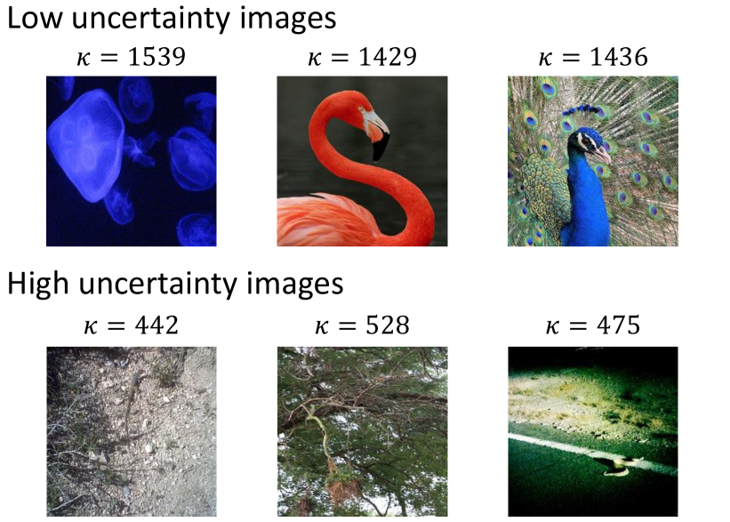
Figure 1: Input images and the predicted uncertainty parameter $\kappa$. Our method learns not only representations of images but also uncertainties in them without supervision. The lower the $\kappa$, the higher the uncertainty. The images with a low $\kappa$ appear to have less salient features than those with a high $\kappa$.

Self-supervised learning (SSL) is a framework for learning representations of data [chen2021exploring, grill2020bootstrap, he2020momentum, chen2021empirical, chen2020simple, zbontar2021barlow, tian2021understanding, newell2020useful, komodakis2018unsupervised, noroozi2016unsupervised]. This method enables training of high-performance models in downstream tasks (e.g., image classification and object detection) without substantial manually labeled data through pre-training the network to generate features. It can mitigate the annotation bottleneck, one of the crucial barriers to the practical application of deep learning. Some state-of-the-art SSL methods, such as SimSiam [chen2021exploring], SimCLR [chen2020simple], and DINO [caron2021emerging], train image encoders by maximizing the similarity between representations of different augmented views of an image.

The probabilistic generative models with variational inference provide another approach for representation learning [kingma2013auto]. This approach learns latent representations in an unsupervised fashion by training inference and generative models (i.e., autoencoders) together. It can naturally incorporate representation uncertainty by formulating them as probabilistic distribution models (e.g., Gaussian). However, the pixel-wise objective for reconstruction is sensitive to rare samples [liu2021self] in such methods. Furthermore, this representation learning is recently found to be less competitive than the SSL methods on the benchmarking classification tasks [liu2021self, newell2020useful]. Although SSL and variational inference seem highly related learning representations without supervision, their theoretical connection has not been fully explored.

In this study, we incorporate the variational inference concept to make the SSL uncertainty-aware and conduct a detailed representation uncertainty analysis. The contributions of this study are summarized as follows.

• We clarify the relationship between SSL (i.e., SimSiam, SimCLR, and DINO) and variational inference, generalizing the SSL methods as the variational inference of spherical or categorical latent variables (§4).

• We derive a novel SSL method called variational inference SimSiam (VI-SimSiam) by incorporating the above relationship. It learns to predict not only representations but also their uncertainty (§ LABEL:sec:our_method).

• We demonstrate that VI-SimSiam successfully estimates uncertainty without labels while achieving competitive classification performance with SimSiam. We qualitatively evaluate the uncertainty estimation capability by comparing input images and the estimated uncertainty parameter $\kappa$, as shown in Fig. 1. In addition, we also describe that the predicted representation uncertainty $\kappa$ is related to the accuracy of the classification task (§ LABEL:sec:experiments).

A comparison of SimSiam and VI-SimSiam is illustrated in Fig. 2, where VI-SimSiam estimates the uncertainty by predicting latent distributions.

2 Related work

2.1 Self-supervised learning

SSL [chen2020simple, he2020momentum, chen2021exploring, grill2020bootstrap, caron2021emerging] has been demonstrated to have notable performance in many downstream tasks, such as classification and object detection. Contrastive SSL methods, including SimCLR[chen2020simple] and MoCo [he2020momentum], learn to increase the similarity of representation pairs augmented from an image (positive pairs) and to decrease the similarity of representation pairs augmented from different images (negative pairs). Conversely, non-contrastive SSL, including SimSiam [chen2021exploring], BYOL [grill2020bootstrap], and DINO [caron2021emerging], learn a model using only the positive pairs. Zbontar et al. [zbontar2021barlow] proposed another non-contrastive method using the redundancy-reduction principle of neuroscience. Furthermore, several studies have theoretically analyzed the SSL methods, such as Tian et al. [tian2021understanding] investigated the reasons behind the superior performance of the non-contrastive methods. Tao et al. [tao2022exploring] claimed that the (non-)contrastive SSL methods can be unified into one form using gradient analysis. Zhang [zhang2022mask] demonstrated a theoretical connection between masked autoencoder [he2022masked] and contrastive learning. However, these studies assumed a deterministic formulation without considering uncertainty in the representations.

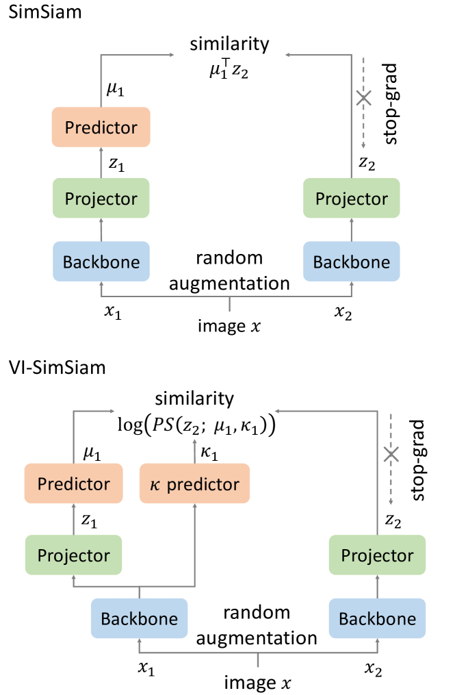
Figure 2: Schematics of VI-SimSiam and SimSiam [chen2021exploring]. These methods use the augmented images $x_{1}$ and $x_{2}$ as input images. In VI-SimSiam, we define the distribution of latent space that follows the Power Spherical distribution [decao2020power]. Unlike SimSiam, VI-SimSiam can predict the representation uncertainty of the image $\kappa$.

2.2 Variational inference

In deep learning, variational inference is generally formulated using auto-encoding variational Bayes [kingma2013auto]. The variational inference estimates latent distributions, such as Gaussian [kingma2013auto], Gaussian mixture [tomczak2018vae], and von Mises-Fischer (vMF) distribution for hyperspherical latent space [davidson2018hyperspherical]. Although Wang et al. [wang2020understanding] pointed out that SSL methods learn representations on the hypersphere, their relevance to the spherical variational inference [davidson2018hyperspherical] has yet to be investigated extensively.

A multimodal variational autoencoder [kurle2019multi, wu2018multimodal, shi2019variational, sutter2021generalized] is trained to infer latent variables from multiple observations from different modalities. The latent variable distribution of multimodal variational inference is often assumed to be the product of experts or the mixture of experts of unimodal distributions [kurle2019multi, wu2018multimodal, shi2019variational]. Sutter et al. [sutter2021generalized] also clarified the connection between them and generalized them as mixture-of-products-of-experts (MoPoE) VAE. Multimodal variational inference seems highly related to the SSL utilizing the multiview inputs. However, their relationship has been unclear.

2.3 Uncertainty-aware methods

Uncertainty-aware methods [der2009aleatory, kendall2017uncertainties, kendall2018multi, mohseni2020self, winkens2020contrastive] have been proposed to solve the problem of learning hindered by data with high uncertainty. Kendall and Gal [kendall2017uncertainties] proposed a method that estimated data uncertainty in regression and classification tasks by assuming that outputs follow a normal distribution. Scott et al. [scott2021mises] proposed a stochastic spherical loss for classification tasks based on the von Mises–Fisher distributions. Additionally, Mohseni et al. [mohseni2020self] and Winkens et al. [winkens2020contrastive] presented methods for estimating uncertainty by combining SSL with a supervised classification task. Uncertainty-aware methods have been proposed for other tasks as well, such as human pose estimation [petrov2018deep, okada2020multi, gundavarapu2019structured], optical flow estimation [ilg2018uncertainty], object detection [he2019bounding, hall2020probabilistic], and reinforcement learning [lutjens2019safe, okada2020planet, guo2021safety].

Several studies have suggested methods to incorporate uncertainty in self-supervised learning of specific tasks [poggi2020uncertainty, pang2020self, xu2021digging, wang2020uncertainty]. Poggi et al. [poggi2020uncertainty] proposed an uncertainty-aware and self-supervised depth estimation. They considered the variance in depth estimated from multiple models as uncertainty. Wang et al. [wang2020uncertainty] demonstrated an uncertainty-aware SSL for three-dimensional object tracking, wherein the ratio of the distances between positive and negative pairs was treated as uncertainty. However, these methods hardly discussed representation uncertainty.

3 Preliminary

The formulations of the SSL methods and variational inference are briefly reviewed in this section.

3.1 Self-supervised learning methods

SimSiam

SimSiam is a non-contrastive SSL method with an objective function that is defined as follows;

$$\mathcal{J}_{\mathrm{SimSiam}}\coloneqq g_{\theta}(x_{1})^{\mathsf{T}}f_{\phi}(x_{2})+g_{\theta}(x_{2})^{\mathsf{T}}f_{\phi}(x_{1}),$$ (1)

where $x_{1}$ and $x_{2}$ are two augmented views of a single image. The term $g_{\theta}$ and $f_{\phi}$ are encoders parameterized with $\theta$ and $\phi$, respectively, and they map the image $x$ to a spherical latent $z\in\mathbb{S}^{d-1}$. In the literature on non-contrastive SSL, the two encoders $g_{\theta}$ and $f_{\phi}$ are referred to as online and target networks, respectively. SimSiam defines the online network $g_{\theta}$ as $g_{\theta}=h_{\theta}\circ f_{\theta}$, where $h_{\theta}$ and $f_{\theta}$ are referred to as a predictor network and projector network [grill2020bootstrap, chen2021exploring], respectively.

SimCLR

The objective function of a contrastive SSL, such as SimCLR is generally described as follows;

$$\mathcal{J}_{\textrm{SimCLR}} \coloneqq\mathcal{J}^{(1,2)}_{\textrm{SimCLR}}+\mathcal{J}^{(2,1)}_{\textrm{SimCLR}},$$

$$\mathcal{J}^{(i,j)}_{\textrm{SimCLR}} \coloneqq\log\frac{\exp(g_{\theta}(x_{i})^{\mathsf{T}}f_{\phi}(x_{j}))}{\sum_{x^{\prime}\in\mathcal{B}}\exp(g_{\theta}(x^{\prime})^{\mathsf{T}}f_{\phi}(x_{j}))}.$$ (2)

where $g_{\theta}(x),f_{\phi}(x)\in\mathbb{S}^{d-1}$, and $\mathcal{B}$ denotes a minibatch.

DINO

DINO is another non-contrastive SSL with an objective and a latent space (i.e., categorical latent) different from those of SimSiam. It is described as;

$$\mathcal{J}_{\textrm{DINO}} \coloneqq-\mathcal{H}(P_{1,\phi},P_{2,\theta})-\mathcal{H}(P_{2,\phi},P_{1,\theta}),$$ (3)

$$P_{i,\phi} \coloneqq\operatorname{softmax}\left(({f_{\phi}(x_{i})-c})/{\tau_{\phi}}\right),$$ (4)

$$P_{j,\theta} \coloneqq\operatorname{softmax}\left({g_{\theta}(x_{j})}/{\tau_{\theta}}\right),$$ (5)

where $\mathcal{H}(P,Q)(=\sum P\log Q)$ denotes cross entropy between two probabilities, $g_{\theta}(x),f_{\phi}(x)\in\mathbb{R}^{d}$, and ($\tau$, $c$) are the parameters for $sharpening$ and $centering$ operations discussed later in § LABEL:sec:dino.

3.2 Multimodal generative model and inference

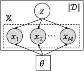
Figure 3: Graphical model.

Fig. 3 shows a graphical model for multimodal generative models, where $\mathcal{D}$ indicates a dataset, $\mathbb{X}=\{x_{i}\}^{M}_{i=1}$ is a set of multimodal observations $x_{i}$, $z$ is a latent variable of the observations, $\theta$ is a deterministic parameter of the generative model $p(\mathbb{X}|z,\theta)$, and $M$ is the number of modalities corresponding to the data augmentation types in this paper. In the SSL context, $\mathbb{X}$ can be regarded as augmented images from stochastic generative processes.

The objective is to find a parameter $\theta^{*}$ that maximizes marginal observation likelihood;

$$\theta^{*} =\mathop{\rm argmax}\limits_{\theta}\mathcal{J}=\mathop{\rm argmax}\limits_{\theta}\mathbb{E}_{p(z)}[\log p(\mathbb{X}|z,\theta)].$$ (6)

Since the marginalization $\mathbb{E}_{p(z)}[\cdot]$ is intractable, we can instead maximize the evidence lower bound (ELBO);

$$\mathbb{E}_{p(z)}[\log p(\mathbb{X}|z,\theta)]\geq\mathcal{J}_{\mathrm{ELBO}}\coloneqq$$

$$=\mathbb{E}_{q(z|\mathbb{X},\phi)}\left[\log p(\mathbb{X}|z,\theta)\right]-D_{\mathrm{KL}}[{q(z|\mathbb{X},\phi)|p(z)}],$$ (7)

where $q(z|\mathbb{X},\phi)$ is a variational inference model parameterized with $\phi$. By optimizing $\mathcal{J}_{\mathrm{ELBO}}$ with respect to both $\theta$ and $\phi$, $q(z|\mathbb{X},\phi)$ approaches the posterior $p(z|\mathbb{X},\theta)$ as the following relation holds;

$$\mathcal{J}-\mathcal{J}_{\mathrm{ELBO}}=D_{\mathrm{KL}}[q(z|\mathbb{X},\phi)|p(z|\mathbb{X},\theta)]\geq 0,$$ (8)

where $D_{\mathrm{KL}}[\cdot]$ is the Kullback-Leibler divergence. Notably, the posterior varies during the optimization process since it depends on the parameterized generative model; i.e., $p(z|\mathbb{X},\theta)\propto p(\mathbb{X}|z,\theta)p(z)$.

4 Self-supervised learning as inference

This section shows a connection between SSL and multimodal variational inference. Usually, a generative model $p(\mathbb{X}|z,\theta)$ and variational inference model $q(z|\mathbb{X},\phi)$ are realized with deep neural networks to solve the problem of Eq. (6), and they are trained via ELBO optimization. Instead, let us consider directly realizing the posterior $p(z|\mathbb{X},\theta)$ as deep neural networks. For this purpose, we remove the generative model term in Eq. (7) by applying Bayes’ theorem;

$$p(\mathbb{X}|z,\theta)=p(z|\mathbb{X},\theta)p(\mathbb{X}|\theta)/\mathbb{E}_{p(\mathbb{X}|\theta)}[p(z|\mathbb{X},\theta)].$$ (9)

Since $p(\mathbb{X}|\theta)$ is intractable, we approximate it with the empirical data distribution $p_{\mathcal{D}}(\mathbb{X})$. Substituting Eq. (9) into Eq. (7) and applying the approximation yields a new objective;

$$\mathcal{J}_{\mathrm{SSL}} \coloneqq\mathcal{J}_{\mathrm{align}}+\mathcal{J}_{\mathrm{uniform}}+\mathcal{J}_{\mathrm{KL}}+p_{\mathcal{D}}(\mathbb{X}),$$

$$\stackrel{{\scriptstyle+}}{{=}}\mathcal{J}_{\mathrm{align}}+\mathcal{J}_{\mathrm{uniform}}+\mathcal{J}_{\mathrm{KL}},$$ (10)

where,

$$\mathcal{J}_{\mathrm{align}}\coloneqq\mathbb{E}_{q(z|\mathbb{X},\phi)}\left[\log p(z|\mathbb{X},\theta)\right],$$ (11)

$$\mathcal{J}_{\mathrm{uniform}}\coloneqq\mathbb{E}_{q(z|\mathbb{X},\phi)}\left[-\log p_{\mathcal{D}}(z|\theta)\right],$$ (12)

$$\mathcal{J}_{\mathrm{KL}}\coloneqq-D_{\mathrm{KL}}[{q(z|\mathbb{X},\phi)|p(z)}],$$ (13)

$$p_{\mathcal{D}}(z|\theta)\coloneqq\mathbb{E}_{p_{\mathcal{D}}(\mathbb{X})}[p(z|\mathbb{X},\theta)].$$ (14)

Furthermore, let $p(z|\mathbb{X},\theta)$ and $q(z|\mathbb{X},\phi)$ respectively be Product-of-Experts (PoE) and Mixture-of-Experts (MoE) of the single modal inference models;

$$p(z|\mathbb{X},\theta) =\eta_{\theta}\prod^{M}_{j=1}p(z|x_{j},\theta),$$ (15)

$$q(z|\mathbb{X},\phi) \coloneqq\frac{1}{M}\sum^{M}_{i=1}q(z|x_{i},\phi),$$ (16)

where $\eta_{\theta}^{-1}\coloneqq\int\prod p(z|x_{j},\theta)dz$ is the renormalization term. Then, we can rewrite $\mathcal{J}_{\mathrm{align}}$ as a form that encourages aligning latent variables from different modals;

$$\mathcal{J}_{\mathrm{align}}= \sum_{i,j}\mathbb{E}_{q(z|x_{i},\phi)}\left[\log p(z|x_{j},\theta)\right]+M\log\eta_{\theta},$$ (17)

Eq. (15) is from Prop. 4.1 described below. Eq. (16) is the definition theoretically validated in [shi2019variational, sutter2021generalized]. Practically, we can ignore unimodal comparisons (i.e., $i=j$) since they provide less effective information.

Proposition 4.1.

Let $p(z)$ be a non-informative prior. The multi-modal posterior $p(z|\mathbb{X},\theta)$ takes the form of PoE of the single-modal posteriors $p(z|x_{j},\theta)$.

Proof.

See Appx. LABEL:appx:proof_poe.

We claim that Eq. (10) generalizes the objectives in Eqs. (1), (2) and (3) as summarized in Table 1. In the rest of this section, we describe how to recover the objectives in the table from Eq. (10). In the derivations, the term $M\log\eta_{\theta}$ is ignored by approximating it as a constant (denoted as $\stackrel{{\scriptstyle+}}{{\simeq}}$).

Table 1: The summary of SSL methods interpreted as variational inference.

	SimSiam [chen2021exploring] (§4.1)	SimCLR [chen2020simple] (§LABEL:sec:simclr_moco)	DINO [tao2022exploring] (§LABEL:sec:dino)	VI-SimSiam (ours) (§LABEL:sec:our_method)
$p(z)$	$\mathcal{U}(\mathbb{S}^{d-1})$		$\mathcal{U}(\Delta^{d-1})$	$\mathcal{U}(\mathbb{S}^{d-1})$
$q(z|x_{i},\phi)$	Deterministic		Categorical	Deterministic
$p(z|x_{j},\theta)$	von-Mises-Fisher		Categorical	Power Spherical
$\mathcal{J}_{\mathrm{align}}$	$z_{{j}}^{\mathsf{T}}z_{{i}}$	$\log\frac{\exp({z_{{j}}^{\mathsf{T}}z_{{i}}})}{\sum_{z}\exp({z^{\mathsf{T}}z_{{i}}})}$	$\sum P_{j}\cdot\log P_{i}$	$\log C_{\mathrm{PS}}(\kappa_{{j}})+\kappa_{{j}}\operatorname{log1p}(z_{j}^{\mathsf{T}}z_{i})$
$\mathcal{J}_{\mathrm{uniform}}$	DirectPred		Centering	DirectPred
$\mathcal{J}_{\mathrm{KL}}$	Const.		Sharpening	Const.
Uncertainty	No		Yes	Yes
aware	(uncertainty parameter $\kappa$ is fixed)		(but has not been discussed)	(uncertainty parameter $\kappa$ is estimated)

4.1 SimSiam as inference

First, we discuss the relationship between SimSiam and the following definition involving the hyperspherical space $\mathbb{S}^{d-1}$.