Bianchi type-V Transitioning model in Brans-Dicke theory with Observational Constraint
Vinod Kumar Bhardwaj1, Archana Dixit2, Anirudh Pradhan3
1,2Department of Mathematics, Institute of Applied Sciences and Humanities, GLA University, Mathura-281 406, Uttar Pradesh, India
3Centre for Cosmology, Astrophysics and Space Science (CCASS), GLA University, Mathura-281 406, Uttar Pradesh, India
1E-mail:dr.vinodbhardwaj@gmail.com
2E-mail:archana.dixit@gla.ac.in
3E-mail:pradhan.anirudh@gmail.com
Abstract
In this paper, we have examined the viability of the Bianchi type-V universe in Brans-Dicke (BD) theory of gravitation. We have discussed the interacting and non-interacting scenarios between dark matter (DM) and dark energy (DE) of the derived universe within the framework of BD theory. CCA technique has been applied to constrain the model parameters using 46 values of observational Hubble data (OHD), Pantheon data (the latest compilation of SNIa with 40 binned in the redshift range and their combined datasets. We establish an exact solution of the field equations to derive the dynamics of the derived universe and the obtained results are found to agree with the observations We also noted a distinctive change in the sign of the deceleration parameter from positive to negative, as well as the presence of a transition red-shift exists. Using various observational data points, the evolution trajectories for diagnostic planes are shown to understand the geometrical behavior of the Bianchi-V model. Some physical properties of the universe are also discussed. It’s also worth noting that the conclusions of the cosmological parameter are consistent with modern observational data.
Keywords : LRS Bianchi-V, Brans-Dicke theory, CDM Model, Statefinders.
PACS: 98.80.-k
1 Introduction
According to recent studies of type Ia supernovae [1, 2] our current universe is undergoing an accelerated phase of expansion proceeded
by a period of deceleration. To examine the current phase of acceleration, a new form of substance with negative pressure, called dark energy, has
been suggested. In literature several models have been examined, to predict cosmic acceleration by assuming dark energy with repulsive gravity as
the major content of the cosmos. According to the Planck observations, Universe’s total mass-energy budget is composed of 68.3 % DE, 26.8 %
dark matter and 4.9 % ordinary matter. This exotic form of energy is known as dark energy which is to be less effective in early times but
dominates at the present epoch. The attracting force of DM is involved in the creation of structure and clustering of galaxies.
Although several observational experiments support DE as a general clarification for the expansion mystery, but there are many questions which
remain unanswered. The cosmological constant () has a repulsive nature, it is a usual candidate for DE. It posseses a low magnitutde in
comparison with prediction of particle physics. Apart from dark energy models, a variety of gravity theories such as f (R) gravity
[3, 4], gravity [5], and gravity [6, 7], gravity [8, 7b], [10], Einstein-Gauss-Bonnet theory [11, 12, 13, 14, 15] were discussed. In the same direction, theory is the
another perspective of modified version of theory of gravity, which has been proposed by Harko et al.[16]. Similaly, many theories such
as “scalartensor theories, scalar field theories, bimetric theories and vector-tensor theories [17, 18], Weyl theory [19],
Lyra theory [20] Ylmaz theory [21] and Brans-Dicke theory [22, 23]” are some examples of these alternative gravitation
theories [24]. For the previous coupled of decades, cosmologists have been interested in alternative theories of gravity, particularly ”scalar-tensor” theories. Among all these alternative theories, the “Brans-Dicke theory (BDT)” is the one of the most successful alternate theory. Alonso et al. [25] have shown that the scalar tensor theory of Brans-Dicke type provides a relativistic generalization of Newtonian gravity in 2+1 dimensions. The theory is metric and test particles follow the space-time geodesics.
BD theory, on the other hand, is often considered as the prototype of a wide category of gravitational theories known as scalar-tensor theories. These theories are derived through a non-minimal coupling between the curvature scalar and a scalar field. These hypotheses have gotten a lot of interest in the cosmology community because they can accurately represent the early expansion of the universe [26]. The BD hypothesis predicts an extended period of inflation to address the universe’s graceful exit dilemma, as outlined by Mathiazhagan and Johri [27], La and Steinhardt [28]. Furthermore, with suitable parameter values, the theory can successfully construct late-time accelerated expansion without the contribution of DE ([29])
Several authors have been explored BD cosmology in different prospectives. The work of Singh and Rai [30] provides a detailed
discussion of Brans-Dick cosmological models. Remarkable studies of BD theory with the application of a non-vanishing cosmological constant
can be seen in [31, 32, 33, 34, 35, 36, 37]. In BD theory, authors [38, 39, 40] studied a model of accelerating universe with
changeable deceleration parameter. In 1984 Brans-Dike cosmological model was investigated by taking . The same idea was further extended
inhomogeneous and anisotropic Bianchi type I spacetime [41, 42].
Akarsu, et al. [43] studied the anisotropic CDM model with Brans–Dicke gravity. Recently, exact solutions of accelerating cosmological models in modified Brans-Dicke theory are proposed [44, 45].
In cosmology, Bianchi-type space-times play a very important role in comprehending and describing the early phases of the universe’s evolution.
The study of Bianchi types II, VIII, and IX universe is particularly relevant since they correlate to well-known solutions such as the FRW
universe with positive curvature, the de Sitter universe, the Taub-NUT solutions, and so on. The Bianchi type-V frame of reference is very
important for developing the models for measuring the expansion of the Universe in its early stages [46, 47]. Several authors [48, 49, 50, 51, 52, 53] have been interested in “Bianchi type-V space-time type over the last decade. The dynamical behavior of the Bianchi-V model is significantly more general than the simple FLRW model. The study of Bianchi type-V cosmological models creates more interest
as these models contain isotropic special cases and permit arbitrarily small anisotropic levels at certain stages [54]. However, we know that,
in recent years, Bianchi cosmological models have become extremely important in observational cosmology, as evidenced by the WMAP observational data.
It has validated an addition to the standard “” model that resembles the Bianchi morphology. The WMAP data analysis supports the
fact that the universe has a preferred direction and it should reach a slightly anisotropic geometry. Therefore, in view of the background anisotropy,
the models with anisotropic backgrounds are more suitable to describe early stages of the universe [55, 56].
Cosmology is now one of the fastest-developing branches of science, particularly in terms of observations. In the last decade, cosmological
data from various sources has been rapidly updated, not only in terms of quantity but also in terms of quality [57]. The latest “CMB anisotropies” results by “Planck Collaboration” provide the precise observations on temperature and polarization of the photons from the last scattering surface near the redshift about [58]. Another observable, which is worthy of mentioning, is the “redshift-space distortion (RSD)”. It has been measured more and more precisely in the past few years. This observable is a key signature to disclose the large-scale structure. In the present study, we proposed transitioning model of the universe Bianchi-V space-time in the framework of BD theory. To achieve the explicit solution for the model, we assumed the scalar field
; where , , , and are constants. In the present study, the recent OHD and Pantheon data sets are used to decide the model parameters“ and [59]. We investigate a transitioning model of the universe for interacting and non-interacting scenarios within the framework of Brans-Dicke theory.
In our derived model, the best fit values of parameters are determined by using statistic. Two observational data sets, i) A data set of 46 OHD and ii) Pantheon data (the latest compilation of SNIa with 40 binned in the redshift range are considered to discuss the dynamics of the derived universe. This paper is structured as follows: In section 2, we introduce the basic field equation of the Bianchi- V universe. In Section 3, we discussed the observational constraints of the model parameter. In Section 4, we have discussed the non-interacting and interacting models. The physical behavior of the model is analyzed in Section 5. In Section 6, we apply the Statefinder diagnostic. Conclusions are mentioned in section 7.
2 Field Equations of Bianchi type-V model
The action for Brans-Dicke theory is given by
| (1) |
where stands for Lagrangian matter field, denotes the Brans-Dicke scalar field and is the Brans-Dicke coupling constant.
The field equations in Brans-Dicke theory [60, 61] by assuming dark matter (DM) and dark energy (DE) are read as:
| (2) |
and
| (3) |
where and
are respectively the energy momentum tensors for DM and DE.
The energy conservation equation is read as
| (4) |
which leads to
| (5) |
We consider the Bianchi type-V metric of the form
| (6) |
where is a constant and the functions , and are the three anisotropic directions of expansion in normal three
dimensional space. Those three functions are equal in FRW models due to the radial symmetry and so we have only one function
there. The average scale factor , the spatial volume and the average Hubble’s parameter
are defined as , , and
respectively.
In a comoving coordinate system, the field equations given by Eqs. (2) and (3), for Bianchi type-V spacetime mentioned in Eq. (6) with energy-momentum tensors defined previously, are read as
| (14) |
| (15) |
Integrating Eq. (11) and omitting constant of integration, we get
| (16) |
here denotes the measures of anisotropy in the Bianchi-V model.
| (18) |
where is the integration constant.
Usng Eq. (2), we can determine the scale factor as .
Thus, we get the following equations finally,
| (19) |
| (20) |
| (21) |
On solving these equation we get dyanamic features of the proposed model.
Authors[62, 63] have considered the funtional relation of Brans-Dicke scalar field and scale factor as
| (22) |
where and are constants. Choice of leads to be consistent with results [64].
The observations of type Ia supernovae [65, 66, 67], “CMB anisotropies” [68], and the
“Planck Collaborations” [69] have verified that the universe is currently expanding speedly, which was decelerating in past. As a result,
the universe must have a “signature flipping” from past deceleration to current acceleration [70, 71]. To determine the
explicit solutions of transitioning universe, we have considered a special parameterization of the Hubble parameter [72, 73, 74]
, where , are constants.
On integration of this parametrization, we get an explicit form of the scale factor as ; where is the constant of integration [59]. The present explicit form of scale factor is an exponential function containing two model parameters and which describe the dynamics of the universe. As , we can have , which provides a non-zero initial value of scale factor for (or a cold initiation of universe with finite volume).
Now, the Brans–Dicke scalar field reads as
| (23) |
The deceleration parameter (DP) is obtained as
| (24) |
Eq. (24) shows that the DP is time-dependent, which can take both positive and negative values representing early decelerating phase and later accelerating phase. From Eq. (24) we can see that as , which is constant and positive for and and for , DP possesses negative value. This indicates that DP has a signature flipping nature from positive to negative era with the evaluation.
By using the relation , we express the cosmological parameters in terms of redshift. Thus, by applying the above transformation, in terms of can be found as . To describe the dynamics of the Universe, the Hubble parameter in terms of redshift can be read as
| (25) |
or
| (26) |
In order to describe the dynamics properties of the model and the bahaviour of physical parameters, we discuss two observational data sets in following section.
3 Observational constraints of the model
3.1 Observational Hubble data set (OHD)
In this section, we have estimate the model parameters and using recent 46 points of the data set (OHD) in the red-shift range and their corresponding standard deviation . These 46 OHD points are summarized in the Table-I [61]-[83]. The best fit value of model parameters and obtained using statistic, which is equivalent to the maximum likelihood analysis given as
| (27) |
where and denote respectively the theoretical and observed value of Hubble parameter . By analysis, we found the values of parameters and , which are comparable with the current Hubble parameter from Planck 2014 results [85].
| References | References | ||||||||
|---|---|---|---|---|---|---|---|---|---|
| 1 | 0 | 67.77 | 1.30 | [75] | 24 | 0.4783 | 80.9 | 9 | [69] |
| 2 | 0.07 | 69 | 19.6 | [76] | 25 | 0.48 | 97 | 60 | [64] |
| 3 | 0.09 | 69 | 12 | [77] | 26 | 0.51 | 90.4 | 1.9 | [68] |
| 4 | 0.01 | 69 | 12 | [64] | 27 | 0.57 | 96.8 | 3.4 | [79] |
| 5 | 0.12 | 68.6 | 26.2 | [76] | 28 | 0.593 | 104 | 13 | [66] |
| 6 | 0.17 | 83 | 8 | [64] | 29 | 0.60 | 87.9 | 6.1 | [70] |
| 7 | 0.179 | 75 | 4 | [66] | 30 | 0.61 | 97.3 | 2.1 | [68] |
| 8 | 0.1993 | 75 | 5 | [66] | 31 | 0.68 | 92 | 8 | [66] |
| 9 | 0.2 | 72.9 | 29.6 | [76] | 32 | 0.73 | 97.3 | 7 | [61] |
| 10 | 0.24 | 79.7 | 2.7 | [78] | 33 | 0.781 | 105 | 12 | [66] |
| 11 | 0.27 | 77 | 14 | [64] | 34 | 0.875 | 125 | 17 | [66] |
| 12 | 0.28 | 88.8 | 36.6 | [76] | 35 | 0.88 | 90 | 40 | [64] |
| 13 | 0.35 | 82.7 | 8.4 | [67] | 36 | 0.9 | 117 | 23 | [64] |
| 14 | 0.352 | 83 | 14 | [66] | 37 | 1.037 | 154 | 20 | [66] |
| 15 | 0.38 | 81.5 | 1.9 | [68] | 38 | 1.3 | 168 | 17 | [64] |
| 16 | 0.3802 | 83 | 13.5 | [69] | 39 | 1.363 | 160 | 33.6 | [80] |
| 17 | 0.4 | 95 | 17 | [77] | 40 | 1.43 | 177 | 18 | [64] |
| 18 | 0.4004 | 77 | 10.2 | [69] | 41 | 1.53 | 140 | 14 | [64] |
| 19 | 0.4247 | 87.1 | 11.2 | [69] | 42 | 1.75 | 202 | 40 | [64] |
| 20 | 0.43 | 86.5 | 3.7 | [78] | 43 | 1.965 | 186.5 | 50.4 | [80] |
| 21 | 0.44 | 82.6 | 7.8 | [70] | 44 | 2.3 | 224 | 8 | [81] |
| 22 | 0.44497 | 92.8 | 12.9 | [69] | 45 | 2.34 | 222 | 7 | [82] |
| 23 | 0.47 | 89 | 49.6 | [71] | 46 | 2.36 | 226 | 8 | [83] |
3.2 Pantheon data
In this part, we fit the Pantheon data (the latest compilation of SNIa with 40 binned in the redshift range to get the best fit values of model parameters and , by minimizing statistic:
| (28) |
“ and ” are represents as the theoretical and observed distance modulus. denotes the standard error of
the observed values.
The distance modulus is read by
| (29) |
where and are “apparent magnitude and absolute magnitude” of any distant luminous object respectively. The parameter and the luminosity distance are defined as
| (30) |
and
| (31) |
The absolute magnitude and apparent magnitude are read as
| (32) |
| (33) |
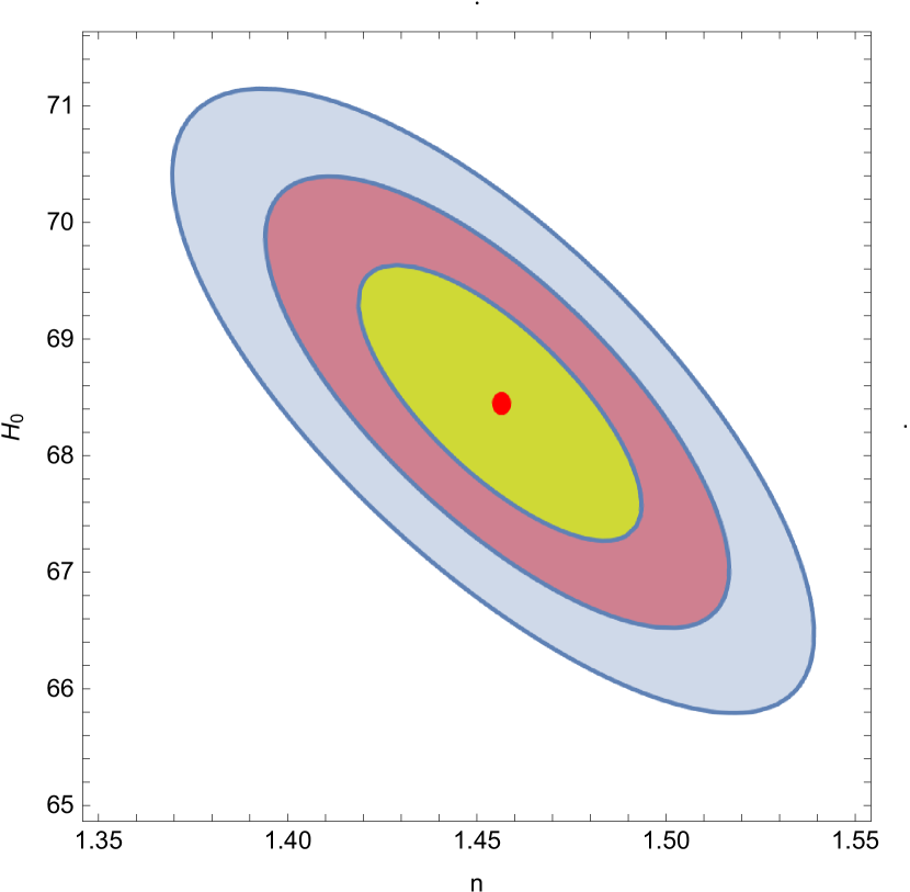
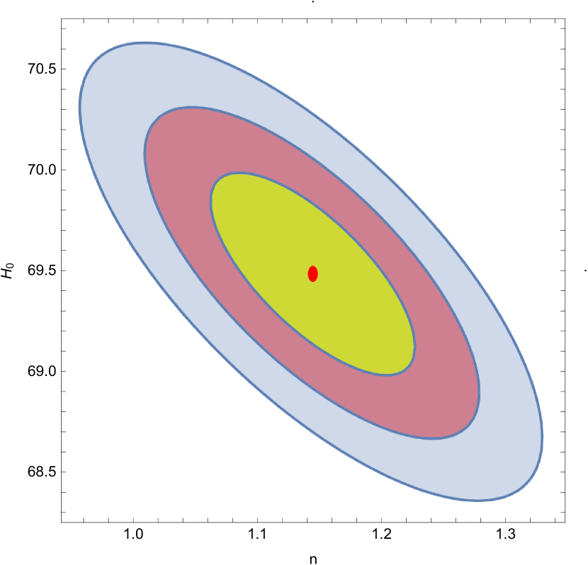
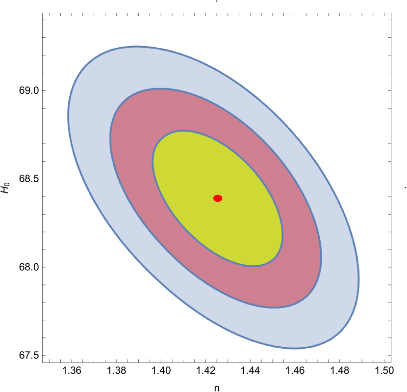
The best fit contour plots for the data set and Pantheon data set and their combined data set are shown in this figures a, b c.
(a)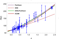 (b)
(b)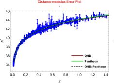
Using a differential age technique and galaxy clustering method, many cosmologists [87, 88] have computed the values of the Hubble constant at various red-shifts. They described several observed Hubble constant Hob values as well as corrections in the range [61, 89]. In our derived model the observed and theoretical values are found to agree quite well, indicating that our model is correct. The dots indicate the 46 observed Hubble constant (Hob) values with corrections, while the linear curves show the theoretical Hubble constant H(z) graphs with marginal corrections.
4 Non-Interacting Model
We suppose that DM and DE only interact gravitationally in the non-interacting model, therefore each source must satisfy the continuity equation independently. Thus, from Eq. (4), we have
| (34) |
| (35) |
The energy density of dark matter is calculated by using Eq. (34)
| (36) |
5 Interacting Model
We discuss the interacting cosmological models of the universe by considering the interaction between DE and DM components. As a result, the DM and DE the continuity equations are written as
| (39) |
| (40) |
The coupling between DM and DE is denoted by . We estimate the coupling between DE and DM as a function of and
, . As a result, for the interaction model, we use “”; is a constant.
Now, the energy densities of DM and DE are determined as follows:
| (41) |
Here, is an integration constant.
| (42) |
For interacting model, the EoS parameter is obtained as:
| (43) |
6 Physical properties and dynamical behaviour of model
The evolution of density parameter for DM and DE are shown in Fig. 3
(a)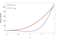 (b)
(b)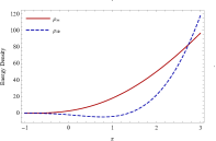 (c)
(c)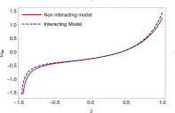
Figure 3(a) shows the energy density for dark matter for the interacting and non-interacting cases with respect to redshift. Figure (3b) shows the variation of energy density for DE versus redshift. In both figures, we conclude that as for (or ) which is consistent with a well-established scenario. From figure 3c, it is clear that the EoS of DE is varying in quintessence region and crossing the Phantom Divide line (PDL) and finally enters in the phantom region in both interacting and non-interacting cases. The curve exhibits a negative tendency before evolving through several stages of acceleration, deceleration, and finally reaching to phantom phase.
The possibility of universe evolution is indicated by the shift from one phase to the next.
6.1 Age of universe
The age of the universe is obtained as
| (44) |
Using Eq. (26), we get
| (45) |
where is the “present age of universe” and it is given by
| (46) |
Integrating Eq.(43), we get
| (47) |
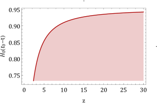
In this study, we have calculated the numerical value of as . Therefore, the present age of the universe for the derived model is obtained as Gyrs. Figure 7 shows the variation of “” with redshift . According to WMAP data [55], the empirical value of current age of the universe is . It’s worth noting that Gyrs is the current age of the universe in Planck collaboration results [90]. The universe’s present has been calculated as Gyrs [105], Gyrs [106] and Gyrs [107] in various cosmological studies.
6.2 Deceleartion parameter
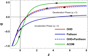
Figure 5 depicts the dynamics of the decelerating parameter with respect to . The models for OHD and (OHD+Pantheon) coincide with CDM with the signature flipping at while for Pantheon data model shows signature
flipping at due to the dominance of DE in the universe. As a result, the current universe evolves with a negative sign of ,
causing the accelerated expansion of the universe. Moreover the reconstruction of is done by the joined , which have obtained the transition redshift and within [91]. which are seen
as well consistent with past outcomes [92, 93, 94, 95, 96] including the expectation . (, joint examination ) [97] is the other limit of transition redshift.
The recent 36 observational Hubble data (OHD) provides the redshift range [98]. The joint light curves (JLA) sample, comprised of 740 type-Ia supernovae (SN Ia) indicates the redshift range . In this way, our developed model depicts a transition from the early deceleration phase to the current speeding phase for OHD, Pantheon, (OHD+Pantheon) data.
Furthermore, we find that the deceleration parameter will remain negative in the future, , .
The DP in terms of the redshift can be written as
| (48) |
6.3 Luminosity Distance
The redshift-luminosity distance connection [99] is a significant observational tool for studying the universe’s evolution.
The luminosity distance is calculated in terms of the redshift, which occurs when light coming out of a distant luminous body is
redshifted due to the expansion of the cosmos. The luminosity distance is used to calculate a source’s flux. It’s written as ,
where denotes the radial coordinate of the source. For the model, the radial coordinate is obtained as
, where .
Therefore, we get the luminosity distance as
| (49) |
6.4 Particle horizon
The particle horizon is a measurement of the size of the observable cosmos [100]. The particle horizon is reads as
| (50) |
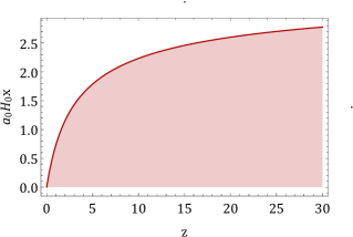
where denotes the ”time in past” at which the light signal is sent from the source. When we integrate Eq. (29) for a large value of red-shift, we get as the particle horizon. Figure 6 depicts the dynamics of correct distance vs red-shift. We can see from Figure 7 that when ), is null, implying that when , the appropriate distance x becomes infinite. Thus we are at very large distance ( at infinite distance) from an event occurred in the beginning of the universe.
7 Statefinder diagnostics
The statefinder pairs are the geometrical quantities that are directly obtained from the metric. This diagnostic is used to distinguish different dark energy models and hence becomes an important tool in modern cosmology. The statefinder parameters and have been defined as follows [101, 102, 103]
| (51) |
| (52) |
| (53) |
(a)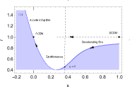 (b)
(b)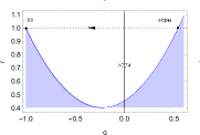 (c)
(c)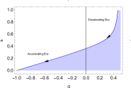
The statefinder diagnostic is a valuable tool in current cosmology used to differentiate various dark energy models [101, 102, 103, 104]. Different trajectories in the and planes express the time evolution for various dark energy models. The present model initially lies in quintessence region (), passes through the CDM and finally approaches to Chaplygin gas region and as clearly seen in Fig.7a. The statefinder pair for CDM and standard cold dark matter(SCDM) are respectively and depicts in the framwork of Bianchi-V background. To get more information on the parametrization, we analyzed the temporal growth of our model by the plane. In Fig. 7(b) The solid line in the diagnostic plane’s shows the evolution of the CDM cosmological model. Initially our model start with the SCDM point passing the CDM point and finally reaches to SS point . The SCDM universe is clearly represented by the and area of the profile. The trajectory begins with a decelerating period and progress to an accelerating era (see Fig.7c).
| Datasets | |||||
|---|---|---|---|---|---|
| 1.457 | 68.46 | -0.2715 | 0.711645 | 31.8169 | |
| Pantheon | 1.144 | 69 | -0.428 | 4.44123 | 569.787 |
| Pantheon | 1.426 | 68.39 | -0.287 | 0.8192 | 628.552 |
8 Conclusion
In this paper, first, we observed the cosmological parameters for the observable universe in Bianchi type V space time in Branc Dicke theory. Second, we used statistical tests to limit the various model parameters of the universe in the resultant model. Table-2 summaries the major findings of the statistical analysis.
The main objective of this article is to use independent observables such as Pantheon dataset, OHD, and their joint combination (OHD+Pantheon) to constrain the free parameters of the theoretical models, which potentially increase the sensitivity of our estimations. Out of these measurements, we specifically discuss the determination. The main features of the derived model are discussed in the following manner:
-
•
First, we have found a perfect solution to Einstein’s field equations for both interacting and non-interacting cases in Bianchi type V space-time.
-
•
We have calculated best-fitted values of the model parameters from the marginal 1, 2, and 3 contour plots of OHD, Pantheon, and (OHD+Pantheon) as shown in Fig.1. The constraints on and for the derived model by fitting the OHD points and the estimate of Hubble’s constant agree closely with Riess et al.[1].
-
•
In Fig. a, we have shown the error bar plots for OHD data set, theoretical model plot for OHD data, and the CDM model. The points with bars indicate the experimental data summarized in Table-1. The 46 points of the and Union 2.1 compilation data are used to constrain the model parameter and . The derived model agrees well with and Pantheon data and closely resembles the behavior of the CDM. The distance modulus error plot of the Pantheon data alongwith the CDM are shown in Figure b.
-
•
Figures 3a and 3b show the graphical behavior of the energy densities for DM and DE. We noticed that and of the model under discussion are positive decreases with time and vary individually with redshift in both interacting and non-interacting scenarios. Figure 3c shows the variation of the DE ( equation of state parameter versus redshift for interacting and non-interacting models.
It has been observed that begins in the positive and ends in the negative. Note that and respectively indicate quintessence and phantom regimes. While represents a universe dominated by cosmological constant. This nature of EoS is ruled out by SN Ia findings. As a result, the evolving range of of our derived model favors the phantom universe in the present epoch.
- •
-
•
In our derived model, there is a smooth transition from decelerating to accelerating phase, which is consistent with the present scenario of the modern cosmology (see Fig. 5). We have plotted the deceleration parameter by getting its numerical solution, which exhibits a transition at , from the early decelerated phase to a late time accelerated phase. This is in good agreement with the current cosmological observations. We have depicted that the deceleration parameter for OHD, (OHD+Pantheon) coincide with the CDM model and have the same transition point(see Fig. 5).
-
•
Particle horizon exists in the derived model, and its value differs from the CDM universe model (see Fig.6). The age of the universe in the developed model matches the empirical value obtained from WMAP measurements and Plank collaborations quite well.
-
•
The variation of the trajectories , and planes are depicted in Fig. 7. In the diagram, the paths of the trajectories are depicted by arrows, which represent various dark energy models, and eventually approach to CDM (see Fig. 7a). The evolution of the trajectories begins at SCDM in the plane diagram, and as time passes, the trajectories of the approach the steady-state model SS (see Fig. 7b). The trajectories begin with a decelerating period and progress to an accelerating era (see Fig. 7c).
We noticed the range of the deceleration parameter from the equation of , which clearly demonstrates the signature flipping behavior. As a result, we find that the current OHD and Pantheon data give well-constrained values, and our model is consistent with recent observations. Furthermore, we describe the dynamics of the cosmos for both interacting and non-interacting scenarios.
Acknowledgments
A. Pradhan is thankful to IUCAA, Pune, India for providing support and facility under Visting Associateship prpgram.
References
- [1] A.G. Riess et al., Astron. J. 116, 1009 (1998).
- [2] S. Perlmutter et al., Astrophys. J. 517, 565 (1999).
- [3] S. Capozziello, Phys. Lett. B 639, 135 (2006).
- [4] S. Carroll, Phys. Rev. D 70, 043528 (2004).
- [5] K. Bamba et al., Astrophys. Space Sci. 342, 155 (2012).
- [6] S. Nojiri, S.D. Odintsov, Phys. Rep. 505, 2 (2011)
- [7] M. F. Shamir, Exp. Theor. Phys, 123, 607 (2016).
- [8] A. Pradhan, D. C. Maurya, A. Dixit, Int. J. Geom. Method Mod. Phys. 18 2150124 (2021).
- [9] A. Banerjee, et al., Europ. Phys. Jour. C 81, 10131 (2021).
- [10] A. Pradhan, A. Dixit, Int. J. Geom. Method Mod. Phys. 18 2150159 (2021).
- [11] S. K. Maurya et al., Mod. Phys. Lett. A 36 2150231 (2021).
- [12] T. Tangphati et al., Mod. Phys. Lett. B 819 136423 (2021).
- [13] T. Tangphati et al., Phys. Dark Univ. 33 100877 (2021).
- [14] S. K. Maurya et al., Europ. Phys. J. C 81 848 (2021).
- [15] G. Panotopoulos et al., Chin. J. Phys. http://doi.org/10.1016/j.cjph.2022.01.008 (2022).
- [16] T. Harko et al., Phys. Rev. D 84, 024020 (2011).
- [17] B. M. Barker, Astrophys. J. 219, 5 (1978).
- [18] J. D. Bekenstein, Phys. Rev. D 70, 083509 (2004).
- [19] H. Weyl, Sitzungsber. Preuss. Akad. Wiss, Berlin 465 (1918).
- [20] G. Lyra, Mathematische Zeitschrift 54, 52 (1951).
- [21] H. Yilmaz, Phys. Rev. 111, 1417 (1958).
- [22] C. Brans, R.H. Dicke, Phys. Rev. 124, 925 (1961).
- [23] A. Pradhan et al., Int. J. Geom. Meth. Modern Phys. 16, 1950185 (1019).
- [24] C. Aktas et al., Phys Lett. B 707, 237 (2012).
- [25] J. L. Alonso, J. L. Cortes, V. Laliena, Phys. Rev. D 67, 024023 (2003).
- [26] A. Guth, Phys. Rev. D 23, 347 (1981).
- [27] C. Mathiazhagan, V.B. Johri, Class. Quantum Gravity 1, L29 (1984).
- [28] D. La, P.J. Steinhardt, Phys. Rev. Lett. 62, 376 (1989).
- [29] N. Banerjee, D. Pavon, Phys. Rev. D 63, 043504 (2001).
- [30] T. Singh, L. N. Rai, Astrophys. Space Sci. 96, 95 (1983).
- [31] C. Romero, A. Barros, Astrophys. Space Sci. 192, 263 (1992).
- [32] K. Uehara and C. W. Kim, Phys. Rev. D 26, 2575 (1982).
- [33] J. M. Servero, P. G. Estevez, Gen. Rel. Grav. 15, 351 (1983).
- [34] D. Lorenz-Petzold, Phys. Rev. D 29, 2399 (1984).
- [35] L.O. Pimentel, Astrophys. Space Sci. 112, 175 (1985).
- [36] T. Etoh, M. Hashimoto, K. Arai, S. Fujimoto, Astron. Astrophys. 325, 893 (1997).
- [37] H. Amirhashchi, A.K. Yadav, Phys. Dark Univ. 30, 100711 (2020).
- [38] S. Das, N. Banerjee, Phys. Rev. D 78, 043512 (2008).
- [39] U. K. Sharma, G. K. Goswami, A. Pradhan, Grav. & Cosmol. 24, 191 (191).
- [40] A. Chand, R. K. Mishra, A. Pradhan, Astrophys. Space Sci. 361, 81 (1985).
- [41] T. Singh, T. Singh, J. Math Phys. 25, 9 (1984).
- [42] A. K. Azad, J. N. Islam, Pramana 60, 2127 (2003).
- [43] O. Akarsu, et al., Europ. Phys. Jour. C 80, 1 (2020).
- [44] P. Mukherjee, S. Chakrabarty, Europ. Phys. Jour. C 79, 681 (2019).
- [45] D. C. Maurya, R. Zia, A. Pradhan, J. Experim. Theor. Phys. 123, 617 (2016.
- [46] V. K. Bhardwaj, M. K. Rana, A. K. Yadav, Astrophys. Space Sci. 364, 1 (2019).
- [47] V. K. Bhardwaj, A. K. Yadav, Int. J. Geom. Methods Mod. Phys. 17(10), 2050159 (2020).
- [48] V. K. Bhardwaj, Mod. Phys. Lett. A 33 1850234 (2018).
- [49] N. Ahmed, A. Pradhan, Int. J. Theor. Phys. 53, 289 (2014).
- [50] H. Amirhashchi, Phys. Rev. D 96, 123507 (2017).
- [51] A. Pradhan, K. Jotania, Int. J. Theor. Phys. 49, 1719 (2010).
- [52] A. Pradhan, H. Amirhashchi, Mod. Phys. Lett. A 26, 2261 (2011).
- [53] A. Pradhan, A. K. Singh, D. S. Chauhan, Int. J. Theor. Phys. 52, 266 (2013).
- [54] C. P. Singh, Braz. J. Phys. 39, 619 (2009).
- [55] G. Hinshaw et al., Astrophys. J. Suppl. 288, 170 (2007).
- [56] G. Hinshaw et al., Astrophys. J. Suppl. 180, 225 (2009).
- [57] A. A. Costa et al., J. Cosmol. Astropart. Phys. 01, 028 (2017).
- [58] R. Adam et al., Astron. Astrophys. 594, A1 (2016).
- [59] R. Nagpal et al., Eur. Phys. J. C 78, 946 (2018).
- [60] A. Pradhan et al., Int. J. Geom. Methods Mod. Phys. 16, 1950185 (2019).
- [61] A. K. Yadav et al., Phys. Dark Universe 31, 100738 (2021).
- [62] A. Sheykhi, Phys. Lett. B 681, 205 (2009).
- [63] V.B. Johari, K. Desikan, Gen. Relativ. Gravit. 26, 1217 (1994).
- [64] D. Stern et al., J. Cosmol. Astropart. Phys. 1002, 008 (2010).
- [65] R. Prasad et al., Int. J. of Mod. Phys. A 36, 2150044 (2021).
- [66] M. Moresco et al., J. Cosmol. Astropart. Phys. 08, 006(2012).
- [67] D. H. Chuang, Y. Wang, Mon. Not. R. Astro. Soc. 435, 255 (2013).
- [68] S. Alam S. et al., Mon. Not. R. Astro. Soc. 470, 2617 (2016).
- [69] M. Moresco et al., J. Cosmol. Astropart. Phys. 05, 014 (2016).
- [70] C. Blake et al., Mon. Not. R. Astro. Soc. 425, 405 (2012).
- [71] A. L. Ratsimbazafy et al., Mon. Not. R. Astro. Soc. 467, 3239 (2017).
- [72] J. P. Singh, Astrophys. Space Sci.318, 103 (2008).
- [73] N. Banerjee, S. Das, Gen. Relat. Gravit. 37, 1695 (2005).
- [74] S.K.J. Pacif et al., Mod. Phys. Lett. A 35(5), 2050011 (2020).
- [75] E. Macaulay et al., Mon. Not. R. Astro. Soc. 486, 2184 (2019).
- [76] C. Zhang et al., Res. Astron. Astrophys. 14, 1221 (2014).
- [77] J. Simon, L. Verde, R. Jimenez, Phys. Rev. D 71, 123001 (2005).
- [78] E. Gazta Naga et al., Mon. Not. R. Astro. Soc. 399, 1663 (2009).
- [79] L. Anderson et al., Mon. Not. R. Astro. Soc. 441, 24 (2014).
- [80] M. Moresco, Mon. Not. R. Astro. Soc. 450, L16 (2015).
- [81] N. G. Busa et al., Astron. Astrophys. 552, A96 (2013).
- [82] T. Delubac et al., Astron. Astrophys. 574, A59 (2015).
- [83] A. Font-Ribera, et al., J. Cosmol. Astropart. Phys. 2014, 027 (2014).
- [84] P. J. Steinhardt, L. M. Wang, I. Zlatev, Phys. Rev. D 59, 123504 (1999).
- [85] P.A.R. Ade et al., [Planck Collaboration], Astro. Astrophys. 571, A16 (2014).
- [86] N. Suzuki et al., Astrophys. J. 746, 85 (2012)
- [87] L. K. Sharma, A. K. Yadav, P. K. Sahoo, B. K. Singh, Results Phys. 10, 738 (2018).
- [88] Y. Chen, S. Kumar, B. Ratra, Astrophys. J. 835, 86 (2017).
- [89] G. K. Goswami, A. Pradhan, A. Beesham, Pramana 93, 1 (2019).
- [90] N. Aghanim et al., Astronomy Astrophysics, 641 A6 (2020).
- [91] A. A. Mamon, Mod. Phys. Lett. A 33, 1850056 (2018).
- [92] R. Nair et al., J. Cosmol. Astropart. Phys. 01, 018 (2012).
- [93] A. A. Mamon, S. Das, Int. J. Mod. Phys. D 25, 1650032 (2016).
- [94] O. Farooq, B. Ratra, Astrophys. J. 766, L7 (2013).
- [95] J. Magana et al., J. Cosmol. Astropart. Phys. 10, 017 (2014).
- [96] A. A. Mamon, K. Bamba and S. Das, Eur. Phys. J. C 77, 29 (2017).
- [97] J. A. S. Lima et al., arXiv: 1205.4688v3[astro-ph.CO] (2012).
- [98] H. Yu, B. Ratra and Fa-Yin Wang, Astrophys. J. 856, 3 (2018).
- [99] A. R. Liddle, D. H. Lyth, Phys. Rep. 231, 1 (1993).
- [100] B. Margalef-Bentabol et al., J. Cosmol. Astropart. Phys. 2013, 015 (2013).
- [101] S. K. J. Pacif, S. Arora, P. K. Sahoo, Phys. Dark Universe 32, 100804 (2021).
- [102] V. Sahni, T. D. Saini, A. A. Starobinsky and U. Alam, JETP Lett. 77, 201 (2003).
- [103] U. Alam et al., Mon. Not. R. Astron. Soc. 344, 1057 (2003).
- [104] M. Sami et al., Phys. Rev. D 86, 103532 (2012).
- [105] H.E. Bond, E.P. Nelan, D.A. VandenBerg, G.H. Schaefer, D. Harmer, Astrophys. J. 765, L12 (2013).
- [106] S. Masi, et al., Prog. Part. Nucl. Phys. 48, 243 (2002).
- [107] A. Renzini, A. Bragaglia, F.R. Ferraro, Astrophys. J. 465, L23 (1996).