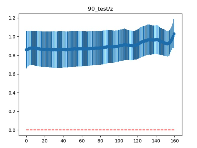
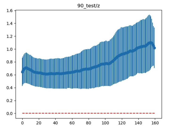
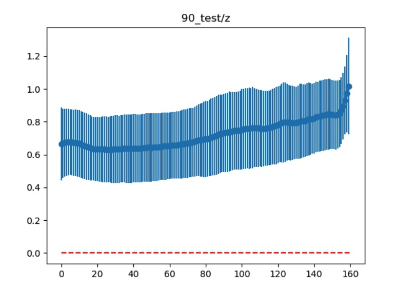
capbtabboxtable[][\FBwidth]
Language modeling via stochastic processes
Abstract
Modern language models can generate high-quality short texts. However, they often meander or are incoherent when generating longer texts. These issues arise from the next-token-only language modeling objective. Recent work in self-supervised learning suggests that models can learn good latent representations via contrastive learning, which can be effective for discriminative tasks. Our work analyzes the application of contrastive representations for generative tasks, like long text generation. We propose one approach for leveraging constrastive representations, which we call Time Control (TC). TC first learns a contrastive representation of the target text domain, then generates text by decoding from these representations. Compared to domain-specific methods and fine-tuning GPT2 across a variety of text domains, TC performs competitively to methods specific for learning sentence representations on discourse coherence. On long text generation settings, TC preserves the text structure both in terms of ordering (up to better) and text length consistency (up to better)111Please find our code at https://github.com/rosewang2008/language_modeling_via_stochastic_processes .
1 Introduction
Large language models (LLM) such as GPT-2 have been extremely successful in text generation (Radford et al., 2019; Brown et al., 2020). However, LLMs are known to generate incoherent long texts. One reason is that they are unable to plan ahead or represent long-range text dynamics (Kiddon et al., 2016; Fan et al., 2019; Hua & Wang, 2020; Duboue & McKeown, 2001; Stent et al., 2004; Tamkin et al., 2020). As a result, they oftentimes produce wandering content with poor discourse structure and low relevance (Hua & Wang, 2020; Zhao et al., 2017; Xu et al., 2020); the text reads as if the model has no anchored goal when generating. These problems with coherence are further exacerbated when forcing autoregressive models to generate longer texts as the model struggles to extrapolate beyond its expected text end point. These problems suggest that LLMs currently fail to properly capture how documents evolve from beginning to end. Doing so is critical for succeeding in goal-oriented tasks such as story, dialog or recipe generation.
Prior work has explored the use of planning-based methods for generating globally coherent text (Kiddon et al., 2016; Fan et al., 2019; Hua & Wang, 2020; Duboue & McKeown, 2001; Stent et al., 2004). However, these methods rely on manually defining text dynamics for specific domains. Other work has attempted to use sentence representations for modeling text, such as with variational auto-encoders (Bowman et al., 2016) or contrastive learning (Gao et al., 2021; Devlin et al., 2019). However, most of these works focus on discriminative tasks like classifying the order of sentences. Methods including van den Oord et al. (2019) have tried decoding from latent contrastive representations, however they fail to generate coherent long sequences.
We propose one way of leveraging contrastive learning representations for generation, which we call Time Control (TC). We begin by assuming that meandering text generated without a goal can be represented as Brownian motion in latent space; this motion enforces the embeddings of neighboring sentences to be similar to each other, whereas those of distant sentences to be dissimilar. Goal-directed behavior can be incorporated into this model by conditioning on a fixed start and end point. In this case, the Brownian motion becomes a Brownian bridge and the resulting latent trajectories abide by simple, closed-form dynamics.
We derive a novel contrastive objective for learning a latent space with Brownian bridge dynamics. We can then use this latent space to generate text that retains local coherence and has improved global coherence. To perform text generation, Time Control first generates a sequence of latent embeddings sampled from the Brownian bridge process pinned at a start and end point. It then conditionally generates sentences using this latent sequence. In our work, we decode the latent sequences by fine-tuning GPT2 to generate text conditioned on Time Control’s latent sequence.
In summary, our work’s contributions are the following:
-
•
We derive a novel contrastive learning objective based on Brownian bridge stochastic processes.
-
•
We explore how contrastive representations can be used in both the discriminative and generative setting with our model Time Control which decodes from these learned representations.
-
•
Across a range of text domains, we show that Time Control generates more or equally coherent text on tasks including forced long text generation , compared to task-specific methods.
-
•
We validate that our latent representations capture text dynamics competitively by evaluating discourse coherence.
-
•
We ablate our method to understand the importance of the contrastive objective, enforcing Brownian bridge dynamics, explicitly modeling latent dynamics, and decoding from a latent plan.
2 Related works
Generating long, coherent text is conceptually difficult for autoregressive models because they lack the ability to model text structure and dynamics (Lin et al., 2021). This means that they struggle to plan and look ahead which leads to generating globally incoherent text. Forcing autoregressive models to generate longer texts exacerbates this incoherence because the models struggle to extrapolate beyond their expected text end point. Prior work has tried to address the problem of generating globally coherent text with planning-based approaches (Puduppully et al., 2019; Moryossef et al., 2019; Fan et al., 2019; Kiddon et al., 2016). However, planning-based approaches rely on domain-specific heuristics for capturing text structure and dynamics.
Our work uses a contrastive objective to learn latent dynamics in text without domain-specific heuristics. Contrastive objectives have been applied to several domains, including language (Devlin et al., 2019; Iter et al., 2020; Liu & Liu, 2021), vision (Chen et al., 2020), and general time series data (Hyvarinen & Morioka, 2016; Hyvarinen et al., 2019). In particular for language, contrastive objectives have been applied to the next-sentence prediction task for improving BERT embeddings (Devlin et al., 2019) and to the discourse coherence setting (Nie et al., 2019; Chen et al., 2019b) for evaluating how coherent pairs of sentences are. However, they are not used for generation and are limited to classification tasks like discourse coherence. Prior work has also tried fitting latent variable models (Bowman et al., 2016), however these generally result in poor language generation (He et al., 2018) or are domain-specific (Weber et al., 2020; Arora et al., 2016).
Our work is closely related to Contrastive Predictive Coding (CPC) from van den Oord et al. (2019). The key difference is CPC implicitly learns unconditioned latent dynamics, whereas our contrastive learning objective imposes goal-conditioned dynamics on our latent space. Additionally, our method builds off of recent findings that contrastive objectives can be used to approximate local transition kernels of stochastic processes (Liu et al., 2021). The main difference between Liu et al. (2021) and our work is that they focus on provable conditions for latent recovery; we focus on empirically effective methods that leverage similar insights for recovering latent representations from language. Finally, our use of stochastic processes draws similarities to diffusion models (Song et al., 2020; Sohl-Dickstein et al., 2015) which apply a chain of diffusion steps onto the data and learn to reverse the diffusion process. However, our application is conceptually different: diffusion processes characterize properties of our latent space and are not a fixed inference method in our work.
3 Methods

This section details our novel contrastive learning objective based on Brownian bridge dynamics. First, we discuss training an encoder via our contrastive learning objective to map sentences to a Brownian bridge (Revuz & Yor, 2013) latent space. Next, we discuss how a decoder learns to reconstruct sentences from this latent space. Finally, we discuss how to generate text at inference time.
3.1 Training an encoder with Brownian bridge dynamics
Our encoder is a nonlinear mapping from raw input space to latent space, . The objective for the encoder is to map high-dimensional sequential data into low-dimensional latents which follow a stochastic process of interest—in this paper, it is the Brownian bridge process. The density of a Brownian bridge process between an arbitrary start point at and end point at is,
| (1) |
This density is intuitive to understand: It acts like a noisy linear interpolation between the start and end point of the trajectory, where should be more like at the start and more like at the end of the trajectory. Uncertainty is highest in the middle region, and low near the end points (rf. Figure 1).
Consider a set of triplet observations, . The goal of our work is to ensure that follow the Brownian bridge transition density in Equation 1. We ensure this using a contrastive objective. Formally, given multiple sequences of data points, , we draw batches consisting of randomly sampled positive triplets where : .222We use indices to denote the start, middle and end point of a Brownian bridge, but these do not correspond to strictly sampling the first, middle and last sentence of a document. can be any sentence in a document as long as comes before and before in the document. Our encoder is optimized by,
| (2) | ||||
| (3) |
is the variance in Equation 1: . Note that Equation 2 sums over negative middle contrasts, . This objective can be viewed as maximizing the extent to which true triplets from the data follow the Brownian bridge process while minimizing the extent to which an alternative mid-point sampled from another sequence does so. 333Empirically, we found Brownian bridge dynamics easier to recover with triplets rather than pairs of contrasts. Appendix O.2 discusses some of the pair-wise contrast results.
Figure 1 illustrates how the objective translates into the language setting for training the encoder. The objective samples triplet sentences from a document. Sentences drawn from the same document make up a smooth latent trajectory; they should be close to each other and follow the conditional density in latent space. Sentences drawn from different documents should not make up a smooth trajectory and should less likely follow bridge dynamics.
Connection to mutual information estimation and triplet classification
We draw connections between our contrastive loss and the mutual information estimation setup from van den Oord et al. (2019); Poole et al. (2019) (as ) and the classification setup from Liu et al. (2021) ().
Following van den Oord et al. (2019); Poole et al. (2019), this objective can be seen as a lower bound on the mutual information between the two end points and the middle point: . Hence, by minimizing the contrastive loss, we are maximizing the amount of information between the trajectory and the linear interpolation of its end points.
Assuming , we can draw a connection to the classification setup studied in Liu et al. (2021). They train a classifier to distinguish in- vs. out-of-order input pairs and show that the Bayes optimal logits for pair-wise classification can be written as a function of the stochastic process transition kernel. This is equivalent to the our loss on a single triplet : . Liu et al. (2021) consider pairs whereas our work considers triplets; we show in Appendix A the pairwise and triplet setups are equivalent.
3.2 Training a decoder with latent plans
Here we discuss how to train a language model to decode latent sequences for generation. We first map all the sentences in the training dataset to our learned latent space using the pretrained encoder . This gives us a Brownian bridge trajectory of sentence-level latent codes for a document in the dataset. Then, rather than learning a decoder from scratch, we fine-tune GPT2 (Radford et al., 2019) to generate text conditioned on past context and the latent plan.
We fine-tune in the following manner. Let be a document with tokens and sentences used to train the decoder. Using the encoder , we can obtain embeddings for each sentence. The decoder is a standard auto-regressive language model that is modified in the following way: at time , the decoder must predict using all tokens in the past , as well as the sentence embedding , where the index is a map which takes each token to its corresponding sentence. This is a form of a reconstruction objective, as the identity of is encoded in .
3.3 Generating text with latent plans at inference time
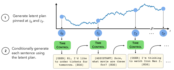
Figure 2 illustrates how the trained decoder generates text at inference time. Given two end points , we sample a trajectory from a latent Brownian bridge, and then generate from the decoder conditioned on this bridge. In many situations, we may not know the endpoints of the Brownian bridge explicitly. In this case, we encode a set of sentences corresponding to start and end points (eg. the first and last sentences of our training set), and fit a Gaussian to these points to form a density estimate. Generating in this case involves first sampling from the Gaussian, and then generating as before from the bridge. More details on training and generation can be found in Appendix C.
4 Experiments
We now evaluate the ability of a model trained with a contrastive objective to capture text dynamics. Specifically, we aim to answer the following research questions (RQ):
- RQ1:
-
Can the contrastive learning objective model local text dynamics? Section 4.1 investigates this question using a sentence ordering prediction task: given two sentences from the same document, we evaluate whether different models can predict their original order.
- RQ2:
-
Can the contrastive learning objective model global text dynamics? Section 4.2 investigates this question on text generation for Wikipedia city articles by examining the length of generated sections.
- RQ3:
-
Can the contrastive learning objective help generate long coherent documents? Section 4.3 investigates this question on forced long text generation: we evaluate how well models preserve global text statistics (such as typical section orders and lengths) when forced to extrapolate during generation.
We run our setup with different latent dimensions (). Our encoder architecture is a frozen, pretrained GPT2 model from Huggingface (Radford et al., 2019; Wolf et al., 2020) and a trainable MLP network. We extract GPT2’s last layer hidden state that corresponds to the end-of-sentence (EOS) token and train the 4-layer MLP on top of the hidden state. The MLP network has intermediate ReLU activations and is trained with stochastic gradient descent with a learning rate of 1e-4 and with momentum 0.9. For more details on the machines we used for our experiments, please refer to Appendix B. This version of the manuscript contains results after correcting for random seeding and GPU nondeterminism. Please refer to Appendix H for details on the version differences.
Encoder ablations
We perform three ablations on our encoder model. Recall that Time Control encoder (A) explicitly models latent structure with (B) Brownian bridge dynamics using a (C) contrastive loss. (A) replaces explicit dynamics with Implicit Dynamics (ID) where future latents are directly predicted with an autoregressive model (van den Oord et al., 2019). (B) replaces Brownian bridge dynamics with Brownian motion (BM): latents follow the transition density in Equation 3. Note is centered at and is not conditioned on a goal end-point. (C) replaces the contrastive loss with a Variational Auto-Encoder (VAE) and centers the priors over to 0 and to 1, as done in our setup. Appendix E includes more detail on the ablations.
Decoder instantiations
We compare two methods for decoding from contrastive representations. The first method decodes from the path as detailed in Section 3.3 by generated by sampling from Brownian bridge or Brownian motion for BM. The second method—which we will call Static—decodes from repititions of the initial latent .
Datasets
We use language datasets that elicit different kinds of structure, from section structure to discourse structure to narrative structure. Time Control does not take in any information about the structure, treating each domain the same under its encoding objective. More information and dataset examples are provided in Appendix F. Wikisection (Arnold et al., 2019) includes Wikipedia articles on cities split by sections. We adapt this dataset such that each article contains four ordered sections (abstract, history, geography, demographics) marked with section id tokens: Each article is represented as, “[ABSTRACT] text [HISTORY] text [GEOGRAPHY] text [DEMOGRAPHICS] text”. Wikihow (WH) (Koupaee & Wang, 2018) contains how-to articles organized by a title, method, and steps. We mark each with its own section id tokens: Each article is represented as “[TITLE] text [METHOD] text [STEP] 1 text [STEP] 2 text …” Recipe NLG (Bień et al., 2020) contains recipes, each with a title, ingredients and set of directions. A recipe is constructed as “[TITLE] text [INGREDIENTS] text [DIRECTIONS] text”. Taskmaster-2 (TM-2) (Byrne et al., 2019) contains conversations on finding restaurants between an assistant and a user. The assistant’s turn is marked with an “[ASSISTANT]” tag, and the user’s turn is marked with a “[USER]” tag. TicketTalk (Byrne et al., 2021) contains conversations on booking movie tickets between an assistant and a user. The assistant’s and user’s turns are similarly marked as in TM-2.
4.1 Modeling local text dynamics
| Wikisection | TM-2 | TicketTalk | ||||
| Method | ||||||
| BERT | ||||||
| ALBERT | ||||||
| S-BERT | ||||||
| Sim-CSE | ||||||
| GPT2 | ||||||
| VAE (8) | ||||||
| VAE (16) | ||||||
| VAE (32) | ||||||
| ID (8) | ||||||
| ID (16) | ||||||
| ID (32) | ||||||
| BM (8) | ||||||
| BM (16) | ||||||
| BM (32) | ||||||
| TC (8) | ||||||
| TC (16) | ||||||
| TC (32) | ||||||
We evaluate how well the Brownian bridge contrastive learning objective models local text dynamics (RQ1) on the discourse coherence setting (Jurafsky, 2000). Discourse coherence is often measured by how well representations capture discourse structure by testing for whether a linear classifier can detect in-order and vs. out-of-order sentence pairs (Chen et al., 2019a). We compare Time Control’s encoder against GPT2’s last layer’s hidden state corresponding to the EOS token (Radford et al., 2019), BERT (Devlin et al., 2019), ALBERT (Lan et al., 2019), Sentence BERT (Reimers et al., 2019), and SimCSE (Gao et al., 2021). The latter 4 methods are designed as sentence embedding models. We also compare to our ablations.
The setup is the following: The encoder takes in two sentences to produce their latents . At random, the latents are fed either in- or out-of-order. A linear classifier is trained on 100 epochs with stochastic gradient descent with a learning rate of 1e-4 and with momentum 0.9. We varied the sentence distance and found that on some domains and for , all methods scored near random accuracy; we have omitted those results in the main paper. Otherwise, the results are summarized in Table 1 where we report the mean and standard error accuracy on a held-out discourse dataset of 3000 examples on 3 runs. Our method is able to compete with sentence embedding specific methods, like ALBERT, BERT, SimCSE. Additionally, though GPT2 is used as a base encoder for Time Control, we observe that Time Control greatly improves upon GPT2 with significant gains on TM-2, TicketTalk, and Wikisection (up to ). Out of all the GPT2-based methods, it performs the best.
Neither VAE nor BM perform better than random accuracy on most of the domains. This suggests that the variational lower bound does not recover the latent embeddings as well as contrastive objectives and the choice of stochastic processes matter for learning informative structural embeddings.
Overall , our model performs competitively on both task-oriented conversations like TM-2 and TicketTalk and enumerative, factual domains like Wikisection . This answers RQ1 in the positive: Time Control can model local text dynamics, like in conversations and articles.
4.2 Modeling global text dynamics
| Method | MM % () |
| GPT2 | |
| SD | |
| SS | |
| VAE (8) | |
| VAE (16) | |
| VAE (32) | |
| Static VAE (8) | |
| Static VAE (16) | |
| Static VAE (32) | |
| ID (8) | |
| ID (16) | |
| ID (32) | |
| Static ID (8) | |
| Static ID (16) | |
| Static ID (32) | |
| BM (8) | |
| BM (16) | |
| BM (32) | |
| Static BM (8) | |
| Static BM (16) | |
| Static BM (32) | |
| TC (8) | |
| TC (16) | |
| TC (32) | |
| Static TC (8) | |
| Static TC (16) | |
| Static TC (32) |
We evaluate how well the Brownian bridge contrastive learning objective models global text dynamics ( RQ2 ) by assessing whether the methods mimic document structure on Wikisection. We check whether the generated section lengths match with the average lengths in the dataset. We focus on Wikisection because it is the only dataset with long, well-defined sections (rf. Appendix F on dataset statistics). Each document contains an abstract, history, geography, and demographics section on a city.
Time Control plans a latent trajectory by running the bridge process between the start and end latent, and . We compare against fine-tuned GPT2. We also include two oracle methods that are fine-tuned GPT2 models with additional section-embedding supervision. One is “sec-dense GPT2” (SD) where each token’s embedding contains the current section identity; section ’s embedding is added onto the token’s positional token embedding. The other is “sec-sparse GPT2” (SS) where the token embedding contains an indicator that is if the token is the start of a new section, and otherwise. For VAE and ID, we calculate the density estimate and and run a linear interpolation between the start and end latents. For BM, we calculate the density estimate and run Brownian motion. Additionally, we run Static for Time Control, VAE, ID, BM which samples and repeatedly decodes from this latent representation. Note that the difference between these Static models is that the decoders are finetuned with their respective objectives (Section 4).
Table 2 reports in percentage how much the generated section lengths deviate from the average section lengths. VAE best matches the section lengths out of all the methods, despite performing at near random accuracy on discourse coherence. We hypothesize that TC does not match the text lengths as well as the VAE method, as the VAE is more explicitly trained to match the text distribution. Nonetheless, TC and Static TC perform competitively with other top-performing baselines like VAE and Static VAE. Another surprising observation was that fine-tuned GPT2, SD and SS mismatch the section lengths by -. Upon further investigation, we noticed the models overshoot short sections and undershoots long sections; this causes the section length deviations. ID and Static ID performs extremely poorly in contrast to these methods; this highlights the challenge of interpolating on learned dynamics models which is exacerbated in the long text generation settings. The results affirm that contrastive objectives can model global text dynamics, such as in matching document structure, however probabilistic objectives like VAE might be a better alternative learning objective.
4.3 Generating globally coherent text
| Method | WH | TM-2 | TT |
| GPT2 | |||
| VAE (8) | |||
| VAE (16) | |||
| VAE (32) | |||
| Static VAE (8) | |||
| Static VAE (16) | |||
| Static VAE (32) | |||
| ID (8) | |||
| ID (16) | |||
| ID (32) | |||
| Static ID (8) | |||
| Static ID (16) | |||
| Static ID (32) | |||
| BM (8) | |||
| BM (16) | |||
| BM (32) | |||
| Static BM (8) | |||
| Static BM (16) | |||
| Static BM (32) | |||
| TC (8) | |||
| TC (16) | |||
| TC (32) | |||
| Static TC (8) | |||
| Static TC (16) | |||
| Static TC (32) |
| Method | Wikisection | Wikihow | TicketTalk | Recipe |
| GPT2 | ||||
| VAE (8) | ||||
| VAE (16) | ||||
| VAE (32) | ||||
| Static VAE (8) | ||||
| Static VAE (16) | ||||
| Static VAE (32) | ||||
| ID (8) | ||||
| ID (16) | ||||
| ID (32) | ||||
| Static ID (8) | ||||
| Static ID (16) | ||||
| Static ID (32) | ||||
| BM (8) | ||||
| BM (16) | ||||
| BM (32) | ||||
| Static BM (8) | ||||
| Static BM (16) | ||||
| Static BM (32) | ||||
| TC (8) | ||||
| TC (16) | ||||
| TC (32) | ||||
| Static TC (8) | ||||
| Static TC (16) | ||||
| Static TC (32) |
We evaluate how well the Brownian bridge contrastive learning objective helps generate globally coherent text (RQ3) where the EOS token is omitted. We refer to this as the forced long text generation setup because the model must extrapolate beyond its natural end point in generation. Appendix D.2 details how the latent plan is generated. For reference, 1000 tokens is about longer than the average Wikisection document (the longest text domain). This setting is intrinsically difficult for auto-regressive models which do not have the ability to “look ahead” during generation (Lin et al., 2021).
We evaluate model extrapolation on two metrics. First is ordering: how well do the models maintain the structure of the document (eg. turn-ordering in TicketTalk)? Second is length consistency. Length consistency captures common failure modes such as a model which stops modeling a conversation between two agents, and instead outputs a long monologue from one agent.
The results are summarized in Table 3 for length consistency and Table 4 for ordering. According to the length consistency metric in Table 3, Static TC maintains text flow the best. Surprisingly, Static TC performs better than TC, which decodes from an actual Brownian bridge sequence. We hypothesize that training the decoder with the contrastive encoder regularizes the model to generate better forced long texts. VAE, BM, ID, and their Static variants do particularly worse than Static TC on length consistency on task-oriented and turn-taking domains like TM-2 and TT, suggesting that the Brownian Bridge objective can model these domains more faithfully. This suggests the importance of good latent dynamics for long text generation. Here, a common failure mode of the nominal GPT2 model is that it produces nonsensical text where it would naturally end generation; this is particularly noticeable on TM-2 and TicketTalk. Figure 5 shows an example of our model’s behavior versus GPT2’s behavior on generating long texts in TicketTalk. The example illustrates how Time Control continues the dialog whereas GPT2 utters nonsensical text.
According to the ordering metric in Table 4, none of the methods surpass the other consistently. These results suggest that that even though Static TC is better at matching text lengths on the forced long text setting, decoding from latent variables to preserve semantically meaningful metrics like section ordering still remains a challenge.
| Time Control : [ USER ] I’m looking for movie tickets please. [ ASSISTANT ] OK, where would you like to see the movie? [ USER ] I’d like to see it at Creek’s End, Oregon please. […] [ ASSISTANT ] Is it OK to go ahead and purchase these tickets? [ USER ] Yeah, that would be great. [ ASSISTANT ] OK. I understand that you are interested in tickets for Emma at AMC Mercado 24 tonight at 7:10pm. Is that OK? [ USER ] Yes, please do that. [ ASSISTANT ] OK |
| GPT2: [ USER ] Hi! Tonight, I’d like to go to the movies. [ ASSISTANT ] Okay. What theater would you like to go to? [ USER ] Center City. […] [ ASSISTANT ] That will be all for now. Thank you for all your help. N/A [ USER ] Bye Bye. [ ASSISTANT ] N/A [ ASSISTANT ] N/A N/A N/A N/A N/A N/A N/A N/A [ USER ] N/A [ ASSISTANT ] N/A N/A N/A [ USER ] N/A [ ASSISTANT ] N/A N/A N/A [ USER ] N/A N/A N/A N/A N/A N/A N/A N/A N/A N/A [ USER ] N/A N/A N/A N/A […] |
5 Discussion on Static and non-Static methods
In an earlier version of this paper, we evaluated the Static methods. Surprisingly, the Static methods perform well despite not leveraging the dynamics at test time. This raises an interesting question of whether there are better ways to leverage contrastive representations at decoding time.
For more details on the differences between the original manuscript and the current manuscript, please refer to Appendix H.
6 Conclusion
Our work explores using representations learned via contrastive learning for generative and discriminative tasks. We propose one way of learning effective language representations which follow Brownian bridge dynamics.
Empirically, we demonstrate this leads to benefits such as simultaneously yielding good representations for discriminative tasks like discourse coherence and generating long texts that preserve section lengths. Future work includes understanding why decoding from a static latent sequence is just as effective—if not more effective—as a dynamic sequence. Additionally, decoding from a latent sequence while preserving other semantically meaningful measures beyond text length still remains a challenge, as suggested by the ordering metrics in the forced long text generation setting. Although our work focuses on benefits of learning stochastic process latents for language generation, our approach can be extended to other domains with sequential data like videos or audio such as in Shin & Wang , or extended to handle arbitrary bridge processes without known fixed start and end points.
7 Reproducibility Statement
In the supplemental, we include a zip file containing our code and processed datasets. We’ve also included in the appendix how we processed the datasets. Our results on showing equivalence between the triplet classification setting and pairwise classification setting are also included in the appendix.
Acknowledgments
REW is supported by the National Science Foundation Graduate Research Fellowship. The authors would give special thanks to CoColab members Mike Wu, Gabriel Poesia, Ali Malik and Alex Tamkin for their support and incredibly helpful discussions. The authors would like to thank the rest of CoCoLab and Rishi Bommasani for reviewing the paper draft. The authors also thank Chris Donahue for helpful pointers on using ILM.
References
- Arnold et al. (2019) Sebastian Arnold, Rudolf Schneider, Philippe Cudré-Mauroux, Felix A. Gers, and Alexander Löser. Sector: A neural model for coherent topic segmentation and classification. Transactions of the Association for Computational Linguistics, 7:169–184, 2019. doi: 10.1162/tacl“˙a“˙00261.
- Arora et al. (2016) Sanjeev Arora, Yuanzhi Li, Yingyu Liang, Tengyu Ma, and Andrej Risteski. A latent variable model approach to pmi-based word embeddings. Transactions of the Association for Computational Linguistics, 4:385–399, 2016.
- Bień et al. (2020) Michał Bień, Michał Gilski, Martyna Maciejewska, Wojciech Taisner, Dawid Wisniewski, and Agnieszka Lawrynowicz. RecipeNLG: A cooking recipes dataset for semi-structured text generation. In Proceedings of the 13th International Conference on Natural Language Generation, pp. 22–28, Dublin, Ireland, December 2020. Association for Computational Linguistics. URL https://www.aclweb.org/anthology/2020.inlg-1.4.
- Bowman et al. (2016) Samuel Bowman, Luke Vilnis, Oriol Vinyals, Andrew Dai, Rafal Jozefowicz, and Samy Bengio. Generating sentences from a continuous space. In Proceedings of The 20th SIGNLL Conference on Computational Natural Language Learning, pp. 10–21, 2016.
- Brown et al. (2020) Tom B Brown, Benjamin Mann, Nick Ryder, Melanie Subbiah, Jared Kaplan, Prafulla Dhariwal, Arvind Neelakantan, Pranav Shyam, Girish Sastry, Amanda Askell, et al. Language models are few-shot learners. arXiv preprint arXiv:2005.14165, 2020.
- Byrne et al. (2019) Bill Byrne, Karthik Krishnamoorthi, Chinnadhurai Sankar, Arvind Neelakantan, Ben Goodrich, Daniel Duckworth, Semih Yavuz, Amit Dubey, Kyu-Young Kim, and Andy Cedilnik. Taskmaster-1: Toward a realistic and diverse dialog dataset. In Proceedings of the 2019 Conference on Empirical Methods in Natural Language Processing and the 9th International Joint Conference on Natural Language Processing (EMNLP-IJCNLP), pp. 4516–4525, 2019.
- Byrne et al. (2021) Bill Byrne, Karthik Krishnamoorthi, Saravanan Ganesh, and Mihir Kale. TicketTalk: Toward human-level performance with end-to-end, transaction-based dialog systems. In Proceedings of the 59th Annual Meeting of the Association for Computational Linguistics and the 11th International Joint Conference on Natural Language Processing (Volume 1: Long Papers), pp. 671–680, Online, August 2021. Association for Computational Linguistics. doi: 10.18653/v1/2021.acl-long.55. URL https://aclanthology.org/2021.acl-long.55.
- Chen et al. (2019a) Mingda Chen, Zewei Chu, and Kevin Gimpel. Evaluation Benchmarks and Learning Criteria for Discourse-Aware Sentence Representations. In Proceedings of the 2019 Conference on Empirical Methods in Natural Language Processing and the 9th International Joint Conference on Natural Language Processing (EMNLP-IJCNLP), pp. 649–662, Hong Kong, China, November 2019a. Association for Computational Linguistics. doi: 10.18653/v1/D19-1060. URL https://www.aclweb.org/anthology/D19-1060.
- Chen et al. (2019b) Mingda Chen, Zewei Chu, and Kevin Gimpel. Evaluation benchmarks and learning criteria for discourse-aware sentence representations. In Proc. of EMNLP, 2019b.
- Chen et al. (2020) Ting Chen, Simon Kornblith, Mohammad Norouzi, and Geoffrey Hinton. A simple framework for contrastive learning of visual representations. In International conference on machine learning, pp. 1597–1607. PMLR, 2020.
- Devlin et al. (2019) Jacob Devlin, Ming-Wei Chang, Kenton Lee, and Kristina Toutanova. BERT: Pre-training of Deep Bidirectional Transformers for Language Understanding. arXiv:1810.04805 [cs], May 2019. URL http://arxiv.org/abs/1810.04805. arXiv: 1810.04805.
- Donahue et al. (2020) Chris Donahue, Mina Lee, and Percy Liang. Enabling language models to fill in the blanks. In Proceedings of the 58th Annual Meeting of the Association for Computational Linguistics, 2020.
- Duboue & McKeown (2001) Pablo A. Duboue and Kathleen R. McKeown. Empirically estimating order constraints for content planning in generation. In Proceedings of the 39th Annual Meeting on Association for Computational Linguistics, ACL ’01, pp. 172–179, USA, 2001. Association for Computational Linguistics. doi: 10.3115/1073012.1073035. URL https://doi.org/10.3115/1073012.1073035.
- Fan et al. (2019) Angela Fan, Mike Lewis, and Yann Dauphin. Strategies for Structuring Story Generation. arXiv:1902.01109 [cs], June 2019. URL http://arxiv.org/abs/1902.01109. arXiv: 1902.01109.
- Gao et al. (2021) Tianyu Gao, Xingcheng Yao, and Danqi Chen. Simcse: Simple contrastive learning of sentence embeddings. arXiv preprint arXiv:2104.08821, 2021.
- He et al. (2018) Junxian He, Daniel Spokoyny, Graham Neubig, and Taylor Berg-Kirkpatrick. Lagging inference networks and posterior collapse in variational autoencoders. In International Conference on Learning Representations, 2018.
- Hua & Wang (2020) Xinyu Hua and Lu Wang. Pair: Planning and iterative refinement in pre-trained transformers for long text generation. In Proceedings of the 2020 Conference on Empirical Methods in Natural Language Processing (EMNLP), pp. 781–793, 2020.
- Hyvarinen & Morioka (2016) Aapo Hyvarinen and Hiroshi Morioka. Unsupervised Feature Extraction by Time-Contrastive Learning and Nonlinear ICA. arXiv:1605.06336 [cs, stat], May 2016. URL http://arxiv.org/abs/1605.06336. arXiv: 1605.06336.
- Hyvarinen et al. (2019) Aapo Hyvarinen, Hiroaki Sasaki, and Richard Turner. Nonlinear ica using auxiliary variables and generalized contrastive learning. In The 22nd International Conference on Artificial Intelligence and Statistics, pp. 859–868. PMLR, 2019.
- Iter et al. (2020) Dan Iter, Kelvin Guu, Larry Lansing, and Dan Jurafsky. Pretraining with Contrastive Sentence Objectives Improves Discourse Performance of Language Models. arXiv:2005.10389 [cs], May 2020. URL http://arxiv.org/abs/2005.10389. arXiv: 2005.10389.
- Jurafsky (2000) Dan Jurafsky. Speech & language processing. Pearson Education India, 2000.
- Kiddon et al. (2016) Chloé Kiddon, Luke Zettlemoyer, and Yejin Choi. Globally coherent text generation with neural checklist models. In Proceedings of the 2016 conference on empirical methods in natural language processing, pp. 329–339, 2016.
- Koupaee & Wang (2018) Mahnaz Koupaee and William Yang Wang. Wikihow: A large scale text summarization dataset. arXiv preprint arXiv:1810.09305, 2018.
- Lan et al. (2019) Zhenzhong Lan, Mingda Chen, Sebastian Goodman, Kevin Gimpel, Piyush Sharma, and Radu Soricut. Albert: A lite bert for self-supervised learning of language representations. arXiv preprint arXiv:1909.11942, 2019.
- Lin (2004) Chin-Yew Lin. ROUGE: A package for automatic evaluation of summaries. In Text Summarization Branches Out, pp. 74–81, Barcelona, Spain, July 2004. Association for Computational Linguistics. URL https://aclanthology.org/W04-1013.
- Lin et al. (2021) Chu-Cheng Lin, Aaron Jaech, Xin Li, Matthew R. Gormley, and Jason Eisner. Limitations of autoregressive models and their alternatives. In Proceedings of the 2021 Conference of the North American Chapter of the Association for Computational Linguistics: Human Language Technologies, pp. 5147–5173, Online, June 2021. Association for Computational Linguistics. doi: 10.18653/v1/2021.naacl-main.405. URL https://aclanthology.org/2021.naacl-main.405.
- Liu et al. (2021) Bingbin Liu, Pradeep Ravikumar, and Andrej Risteski. Contrastive learning of strong-mixing continuous-time stochastic processes. arXiv:2103.02740 [cs, stat], March 2021. URL http://arxiv.org/abs/2103.02740. arXiv: 2103.02740.
- Liu & Liu (2021) Yixin Liu and Pengfei Liu. SimCLS: A Simple Framework for Contrastive Learning of Abstractive Summarization. In Proceedings of the 59th Annual Meeting of the Association for Computational Linguistics and the 11th International Joint Conference on Natural Language Processing (Volume 2: Short Papers), pp. 1065–1072, Online, August 2021. Association for Computational Linguistics. doi: 10.18653/v1/2021.acl-short.135. URL https://aclanthology.org/2021.acl-short.135.
- Moryossef et al. (2019) Amit Moryossef, Yoav Goldberg, and Ido Dagan. Step-by-step: Separating planning from realization in neural data-to-text generation. In Proceedings of the 2019 Conference of the North American Chapter of the Association for Computational Linguistics: Human Language Technologies, Volume 1 (Long and Short Papers), pp. 2267–2277, Minneapolis, Minnesota, June 2019. Association for Computational Linguistics. doi: 10.18653/v1/N19-1236. URL https://aclanthology.org/N19-1236.
- Mostafazadeh et al. (2016) Nasrin Mostafazadeh, Nathanael Chambers, Xiaodong He, Devi Parikh, Dhruv Batra, Lucy Vanderwende, Pushmeet Kohli, and James Allen. A corpus and cloze evaluation for deeper understanding of commonsense stories. In Proceedings of the 2016 Conference of the North American Chapter of the Association for Computational Linguistics: Human Language Technologies, pp. 839–849, San Diego, California, June 2016. Association for Computational Linguistics. doi: 10.18653/v1/N16-1098. URL https://aclanthology.org/N16-1098.
- Nie et al. (2019) Allen Nie, Erin Bennett, and Noah Goodman. DisSent: Learning Sentence Representations from Explicit Discourse Relations. In Proceedings of the 57th Annual Meeting of the Association for Computational Linguistics, pp. 4497–4510, Florence, Italy, July 2019. Association for Computational Linguistics. doi: 10.18653/v1/P19-1442. URL https://www.aclweb.org/anthology/P19-1442.
- Papineni et al. (2002) Kishore Papineni, Salim Roukos, Todd Ward, and Wei-Jing Zhu. Bleu: a method for automatic evaluation of machine translation. In Proceedings of the 40th annual meeting of the Association for Computational Linguistics, pp. 311–318, 2002.
- Poole et al. (2019) Ben Poole, Sherjil Ozair, Aaron Van Den Oord, Alex Alemi, and George Tucker. On variational bounds of mutual information. In International Conference on Machine Learning, pp. 5171–5180. PMLR, 2019.
- Puduppully et al. (2019) Ratish Puduppully, Li Dong, and Mirella Lapata. Data-to-text generation with content selection and planning. In Proceedings of the AAAI conference on artificial intelligence, volume 33, pp. 6908–6915, 2019.
- Radford et al. (2019) Alec Radford, Jeff Wu, Rewon Child, David Luan, Dario Amodei, and Ilya Sutskever. Language models are unsupervised multitask learners. 2019.
- Reimers et al. (2019) Nils Reimers, Iryna Gurevych, Nils Reimers, Iryna Gurevych, Nandan Thakur, Nils Reimers, Johannes Daxenberger, Iryna Gurevych, Nils Reimers, Iryna Gurevych, et al. Sentence-bert: Sentence embeddings using siamese bert-networks. In Proceedings of the 2019 Conference on Empirical Methods in Natural Language Processing. Association for Computational Linguistics, 2019.
- Revuz & Yor (2013) Daniel Revuz and Marc Yor. Continuous martingales and Brownian motion, volume 293. Springer Science & Business Media, 2013.
- Sellam et al. (2020) Thibault Sellam, Dipanjan Das, and Ankur P. Parikh. Bleurt: Learning robust metrics for text generation, 2020.
- (39) Harry Donghyeop Shin and Rose E Wang. Clap: Conditional latent planners for offline reinforcement learning. In NeurIPS 2022 Foundation Models for Decision Making Workshop.
- Sohl-Dickstein et al. (2015) Jascha Sohl-Dickstein, Eric Weiss, Niru Maheswaranathan, and Surya Ganguli. Deep unsupervised learning using nonequilibrium thermodynamics. In International Conference on Machine Learning, pp. 2256–2265. PMLR, 2015.
- Song et al. (2020) Yang Song, Jascha Sohl-Dickstein, Diederik P Kingma, Abhishek Kumar, Stefano Ermon, and Ben Poole. Score-based generative modeling through stochastic differential equations. In International Conference on Learning Representations, 2020.
- Stent et al. (2004) Amanda Stent, Rashmi Prasad, and Marilyn Walker. Trainable sentence planning for complex information presentation in spoken dialog systems. In Proceedings of the 42nd Annual Meeting on Association for Computational Linguistics, ACL ’04, pp. 79–es, USA, 2004. Association for Computational Linguistics. doi: 10.3115/1218955.1218966. URL https://doi.org/10.3115/1218955.1218966.
- Tamkin et al. (2020) Alex Tamkin, Dan Jurafsky, and Noah Goodman. Language through a prism: A spectral approach for multiscale language representations. Advances in Neural Information Processing Systems, 33:5492–5504, 2020.
- van den Oord et al. (2019) Aaron van den Oord, Yazhe Li, and Oriol Vinyals. Representation learning with contrastive predictive coding, 2019.
- Weber et al. (2020) Noah Weber, Leena Shekhar, Heeyoung Kwon, Niranjan Balasubramanian, and Nathanael Chambers. Generating narrative text in a switching dynamical system. In Proceedings of the 24th Conference on Computational Natural Language Learning, pp. 520–530, 2020.
- Wolf et al. (2020) Thomas Wolf, Lysandre Debut, Victor Sanh, Julien Chaumond, Clement Delangue, Anthony Moi, Pierric Cistac, Tim Rault, Rémi Louf, Morgan Funtowicz, Joe Davison, Sam Shleifer, Patrick von Platen, Clara Ma, Yacine Jernite, Julien Plu, Canwen Xu, Teven Le Scao, Sylvain Gugger, Mariama Drame, Quentin Lhoest, and Alexander M. Rush. Transformers: State-of-the-art natural language processing. In Proceedings of the 2020 Conference on Empirical Methods in Natural Language Processing: System Demonstrations, pp. 38–45, Online, October 2020. Association for Computational Linguistics. URL https://www.aclweb.org/anthology/2020.emnlp-demos.6.
- Xu et al. (2020) Jiacheng Xu, Zhe Gan, Yu Cheng, and Jingjing Liu. Discourse-aware neural extractive text summarization. In Proceedings of the 58th Annual Meeting of the Association for Computational Linguistics, pp. 5021–5031, Online, July 2020. Association for Computational Linguistics. doi: 10.18653/v1/2020.acl-main.451. URL https://aclanthology.org/2020.acl-main.451.
- Zhang et al. (2019) Tianyi Zhang, Varsha Kishore, Felix Wu, Kilian Q Weinberger, and Yoav Artzi. Bertscore: Evaluating text generation with bert. In International Conference on Learning Representations, 2019.
- Zhao et al. (2017) Tiancheng Zhao, Ran Zhao, and Maxine Eskenazi. Learning discourse-level diversity for neural dialog models using conditional variational autoencoders. In Proceedings of the 55th Annual Meeting of the Association for Computational Linguistics (Volume 1: Long Papers), pp. 654–664, Vancouver, Canada, July 2017. Association for Computational Linguistics. doi: 10.18653/v1/P17-1061. URL https://aclanthology.org/P17-1061.
Appendix A Showing the equivalence of the pairwise and triplet classification task
In this section, we focus on the classification setup where the goal is to train a classifier to detect in- vs. out-of-order groups of inputs. Specifically, we want to show that the classification setup from Liu et al. (2021) where the inputs come in pairs is equivalent to the setup where the inputs come in triplets. The triplet inputs are what we assume for Time Control.
Notation
We denote latent space as ; we typically do not observe this space directly. We denote the observation space as ; this is the space we observe directly.
We define the Brownian bridge for as
| (4) |
where is a standard Wiener process, .
We state the assumptions:
-
•
We assume latents are drawn from the Brownian bridge process defined by the stochastic differential equation,
(5) The intervals at which latents are sampled are every step: .
-
•
We denote the transition probabilities as
(6) We denote the proposal distribution over possible intermediate triplets .
Liu et al. (2021) characterize properties of an optimal classifier which observes pairs of latents and it outputs in , a probability indicating whether the pair comes in order (ie. ) or not in order (ie. a randomly sampled latent). They train using an L2 loss, .
Lemma 1 of their work states the following : The optimum of the contrastive learning objective satisfies
| (7) |
Manipulating this equality, we observe that the transition kernel has the following relation to the classifier which takes in pairs of observations,
| (8) | ||||
| (9) |
Our setting however assumes that the algorithm receives triplets of data points, . We want to show below that minimizing with triplet contrasts in the classification setting still approximates the transition kernel. In particular, we’re interested in transitions of a Brownian bridge pinned at : .
Let’s say we have two positive triplet samples, and , where . Following Liu et al. (2021), minimizing yields the following on each triplet:
| (10) | ||||
| (11) |
| (12) |
Similar to the pair-wise classification setting, we’ve shown that minimizing in the triplet classification setting results in approximating the transition kernel of the Brownian bridge process.
Appendix B Machines used for training
We found that our decoding results are sensitive to the GPU machine type. For example, in the length mismatch results in Table 2, TC (8) had a deviation of in one set of three seeds and a deviation of in another set of three seeds. In light of this, we randomized over the choice of machines. These machines include: RTX A6000, RTX A5000, GeFORCE RTX 3090, TITAN RTX, TITAN Xp, TITAN V, and GeForce GTX TITAN X machines.
Appendix C Training details
Here we describe the training procedure for the encoder and the fine-tuning procedure for decoding.
Brownian bridge encoder
The encoder architecture is a frozen, pretrained GPT2 model from Huggingface (Radford et al., 2019; Wolf et al., 2020) and a trainable MLP network. We extract the GPT2’s last layer hidden state that corresponds to the end-of-sentence (EOS) token and train the 4-layer MLP on top of the hidden state. The MLP network has intermediate ReLU activations and is trained with stochastic gradient descent with a learning rate of 1e-4 and with momentum 0.9. We train the encoder for 100 epochs on each of the datasets.
The text fed into GPT2 are fed in on a sentence level. This means that the input refers to the ’th sentence of a document. The sentences are separated from each other in the main text as “ . ” which is added to the tokenizer as a separate token for indexing convenience.
Fine-tuning GPT2 with latent embeddings
After training the encoder, we run it on the training dataset to collect an accompanying latent trajectory for each text. The encoder is run on the dataset at a sentence level: we separate the text by sentences and pass the sentences through the encoder.
The sentence latent embeddings are aligned with the tokens of that sentence and offset by one token before the start of that sentence token. Let’s illustrate by an example. We denote [SOS] as the start of the document token, [s1] as sentence 1 tokens and [s2] as sentence 2 tokens. [ . ] is the period token which we’ve added into the tokenizer. denote the latent variable corresponding to the ’th sentence.
Let’s say that the sequence fed into GPT2 is “[SOS] [s1] [s1] [s1] [ . ] [s2] [s2] [s2]”. Then the corresponding latent trajectory is “”. The latent variables are added onto the positional embeddings. We then fine-tune GPT2 as normal.
Appendix D Generation with embeddings
D.1 Normal text generation
We first sample a start and end latent, where are calculated as the density estimates over the training dataset. We pin our trajectory to the start and end latent, and run the Brownian bridge using a first-order approximation. For normal long text generation, we set to be the average number of sentences in each of the dataset. For forced long text generation, we set to be proportional to the number of sentences needed in order to generate 1000 tokens. By the end, we have a trajectory .
Generation starts with feeding the SOS token and the first latent . Once GPT2 emits a [ . ] token and terminates sentence , we transition to the next latent . This process continues until GPT2 is finished with generation. If GPT2 generates more sentences than there are latents in the trajectory, the last latent is used until the end of generation.
D.2 Forced long text generation
Let denote the average number of sentences in a document and denote the average number of tokens in a document. Rather than planning a trajectory of length (the average number of sentences in a document) which is what is done in Section 4.3 for normal text generation, we scale the trajectory length to . is determined by how many more tokens we need in order to fill up to GPT-2 maximum context length of 1024: .
Appendix E Ablations
The following methods ablate the encoder model in Time Control; in other words, the ablations dissect the assumptions we make in the first step of Time Control described in Section 3.1. Recall that Time Control (A) explicitly models latent structure with (B) Brownian bridge dynamics using a (C) contrastive loss. (A) replaces explicit dynamics with Implicit Dynamics (ID) where future latents are directly predicted with an autoregressive model (van den Oord et al., 2019). (B) replaces Brownian bridge dynamics with Brownian motion (BM) which doesn’t rely on pinning trajectories. Latents follow the transition density . (C) replaces the contrastive loss with the Variational Auto-Encoder (VAE). Below we detail how these ablations are implemented.
E.1 Implicit Dynamics (ID)
The Implicit Dynamics ablation is where we compare our explicit dynamics objective to van den Oord et al. (2019) which suggests an implicit latent dynamics objective. This ablation thus changes the learned latent dynamics. In van den Oord et al. (2019), they train two models. One is a non-linear encoder which takes observation (eg. a sentence) and maps it to a latent representation . Two is an autoregressive context model which summarizes a sequence of latent variables into a context latent representation . Rather than directly predicting a future observation ( steps from the current timestep ), they model the density ratio that preserves the mutual information between and the context variable :
| (13) |
They model this with a log-bilinear model which applies a linear transformation for modelling latents k-steps away from timestep . This way, they avoid directly learning the generative model .
They train both models jointly via a contrastive InfoNCE loss. Given a set of random samples (eg. sentences from different documents) containing one positive sample from and negative samples from a proposal distribution , they optimize:
| (14) |
The encoder for Implicit Dynamics has the same architecture as Time Control. The context encoder using a 2400-hidden-unit GRU, as done in van den Oord et al. (2019). We then train both encoders using the InfoNCE loss, as done in prior work. Since and are trained to align latents up to a linear rotation, we use for extracting the sentence embeddings.
E.2 Brownian motion (BM)
The Brownian motion ablation is where we remove goal-conditioning in the dynamics. The main change is in distance function in Equation 3. BM instead optimizes the following equation:
| (15) |
where is the variance in of the Wiener process, .
E.3 Variational Auto-Encoder (VAE)
The Variational Auto-Encoder ablation is where we compare our contrastive objective with a variational one. This ablation changes the encoder objective from Section 3.1 from Equation 2 to the ELBO objective. Below we derive the ELBO objective. Similar to the contrastive objective, we’re deriving the ELBO over the triplet dynamics in the Brownian bridge.
We assume the priors over is 0-centered and is 1-centered, which is similar to our Brownian Bridge setup. The encoder is parameterized with the same architecture as our encoder. The decoder is a fine-tuned GPT2 model.
E.4 Static decoding
Static impacts how the latent plans are generated for the methods at inference time. Instead of generating the latent plan by running the Brownian bridge dynamics (applicable to VAE, ID, and TC) or Brownian motion (applicable to BM), the method generates the plan of the same length and decodes from this plan.
Appendix F Dataset information
For each dataset, text examples were filtered out if they did not fit within GPT2’s context length of 1024 tokens. We also added the token “ . ” for each setting to mark the end of a sentence. This was done for indexing purposes, eg. when aligning the latent embeddings.
Wikisection
(Arnold et al., 2019) includes Wikipedia articles on cities split by sections. We adapt this dataset such that each article contains four ordered sections (abstract, history, geography, demographics) marked with section id tokens: Each article is represented as, “[ABSTRACT] text [HISTORY] text [GEOGRAPHY] text [DEMOGRAPHICS] text”. These section id tokens are added to the tokenizer.
The training dataset contains 1420 articles. The section lengths have the following breakdown measured in the number of BPE tokens (GPT2 tokenizer):
-
•
Abstract:
-
•
History:
-
•
Geography:
-
•
Demographics:
The test dataset contains 431 articles. The section lengths have a similar breakdown:
-
•
Abstract:
-
•
History:
-
•
Geography:
-
•
Demographics:
The ordering metric used in Table 4 is if all four section ids occur exactly once and come in the order as they are listed above.
The length mismatch in used in Table 2 is calculated with respect to the training set lengths.
Wikihow
(Koupaee & Wang, 2018) contains how-to articles organized by a title, method, and steps. Each article includes multiple methods for completing a multi-step procedural task such as “How to Register to Vote”. We scraped all the available English articles covering a wide range of topics following Koupaee & Wang (2018). We mark each with its own section id tokens: Each article is represented as “[TITLE] text [METHOD] text [STEP] 1 text [STEP] 2 text …”
The training dataset contains 1566 articles. The section lengths are,
-
•
Title:
-
•
Method:
-
•
Steps (total step length):
The test dataset contains 243 articles. The section lengths are,
-
•
Title:
-
•
Method:
-
•
Steps (total step length):
The ordering metric used in Table 4 is if all the section ids appear in order, the TITLE and METHOD section ids are not repeated, and the step numbers come in order. It’s otherwise.
The deviation in section length measured in Table 3 is calculated with respect to the training set lengths. We check for whether the models are able to maintain the section lengths when it has to extrapolate. The most common failure mode is that the model generates incoherent text and allocates this text to the last section of what it’s generated thus far, resulting in the deviation in section lengths.
Recipe NLG
(Bień et al., 2020) contains recipes, each with a title, ingredients and set of instructions. A recipe is constructed as “[TITLE] text [INGREDIENTS] text [DIRECTIONS] text”.
The training dataset contains 4000 recipes. The section lengths are,
-
•
Title:
-
•
Ingredients:
-
•
Directions (total step length):
The test dataset contains 1000 recipes. The section lengths are,
-
•
Title:
-
•
Ingredients:
-
•
Directions (total step length):
The ordering metric used in Table 4 is if all the section ids appear exactly once and in order. It’s otherwise.
Taskmaster-2
(TM-2) (Byrne et al., 2019) which contains conversations on finding restaurants between an assistant and a user. The assistant’s turn is marked with an “[ASSISTANT]” tag, and the user’s turn is marked with a “[USER]” tag.
The training dataset contains 2000 conversations. The section lengths are,
-
•
User:
-
•
Assistant:
The test dataset contains 1276 conversations. The section lengths are,
-
•
User:
-
•
Assistant:
The ordering metric used in Table 4 does not apply here because the user and assistant don’t take turns in the dialog.
The deviation in section length measured in Table 3 is calculated with respect to the training set lengths. We check for whether the models are able to maintain the utterance lengths between the user and assistant when it has to extrapolate. The most common failure mode is that the model generates incoherent text and allocates this text to the last section of what it’s generated thus far, resulting in the deviation in section lengths.
TicketTalk
(Byrne et al., 2021) which contains conversations on booking movie tickets between an assistant and a user. The assistant’s and user’s turned are similarly marked as in TM-2.
The training dataset contains 2000 conversations. The section lengths are,
-
•
User:
-
•
Assistant:
The test dataset contains 1276 conversations. The section lengths are,
-
•
User:
-
•
Assistant:
The deviation in section length measured in Table 3 is calculated similarly to TM-2.
The ordering metric used in Table 4 applies because the user and assistant take turns in the dialog. The ordering metric is if the user and assistant take turns in the conversation. It’s otherwise.
ROC Stories
(Mostafazadeh et al., 2016) is a short stories dataset. Each story contains 5 sentences. No additional tokens are added in this dataset. The training dataset contains 2000 stories, and the test dataset contains 1000 stories. This dataset was used in the original text infilling experiments we had. Those previous results are in Table 21, Table 11 and Table 12.
Appendix G Perplexity after fine-tuning
| Method | Wikisection | Wikihow | TM-2 | TicketTalk | Recipe |
| GPT2 | |||||
| sec-dense | |||||
| sec-sparse | |||||
| VAE (8) | |||||
| VAE (16) | |||||
| VAE (32) | |||||
| ID (8) | |||||
| ID (16) | |||||
| ID (32) | |||||
| BM (8) | |||||
| BM (16) | |||||
| BM (32) | |||||
| TC (8) | |||||
| TC (16) | |||||
| TC (32) |
Table 6 reports the final perplexity scores after fine-tuning GPT2 on the different domains with the methods. We fine-tune for 10 epochs and checkpoint the models every 1000 steps; we keep the model checkpoint that scores the lowest PPL on a held-out validation set.
Appendix H Differences in the corrected manuscript
This section discusses updates and differences from an earlier version of this paper due to correcting bugs during a post-publication code review and re-running experiments. Sources of randomness, such as the behavior of the torch dataloader, GPU nondeterminism, and Weights and Biases logging have caused some differences in the experimental outcomes even in cases where there were no bugs. To make the differences clear, we highlight both original and current results, as well as a short explanation of any differences. The numbers reported in the main text correspond to the current version of the codebase available at https://github.com/rosewang2008/language_modeling_via_stochastic_processes with version hash: 95ded1e82f904e1c2dbce5701f54ab880a1a1e62.
H.1 Discourse coherence
For reference, Table 7 shows both the original and new results. The original results are marked with Original.
Differences
In the previous version, ALBERT, SimCSE and TC were competitive with each other. In the updated version, BERT is competitive with these methods as well. TC is the most competitive out of all the GPT2-based models.
Cause
This discrepancy is due to a wandb step logging issue where wandb previously only reported on early training epochs. Therefore, the previous discourse coherence results generally under-report the actual performance–this particularly impacts Wikisection. In general, all methods improve and do better than random accuracy after resolving this issue.
| Wikisection | TM-2 | TicketTalk | ||||
| Method | ||||||
| Original BERT | ||||||
| Original ALBERT | ||||||
| Original S-BERT | ||||||
| Original Sim-CSE | ||||||
| BERT | ||||||
| ALBERT | ||||||
| S-BERT | ||||||
| Sim-CSE | ||||||
| Original GPT2 | ||||||
| GPT2 | ||||||
| Original VAE (8) | ||||||
| Original VAE (16) | ||||||
| Original VAE (32) | ||||||
| VAE (8) | ||||||
| VAE (16) | ||||||
| VAE (32) | ||||||
| Original ID (8) | ||||||
| Original Original ID (16) | ||||||
| Original ID (32) | ||||||
| ID (8) | ||||||
| ID (16) | ||||||
| ID (32) | ||||||
| Original BM (8) | ||||||
| Original BM (16) | ||||||
| Original BM (32) | ||||||
| BM (8) | ||||||
| BM (16) | ||||||
| BM (32) | ||||||
| Original TC (8) | ||||||
| Original TC (16) | ||||||
| Original TC (32) | ||||||
| TC (8) | ||||||
| TC (16) | ||||||
| TC (32) | ||||||
H.2 Length mismatch
For reference, Table 8 shows both the original and new results. The original results are marked with Original.
Differences
In the previous version, TC performed the best. In the updated version, Static VAE performs the best, followed by Static TC.
Causes
The variability is caused by the dataset loader being seeded separately from usual seeding sources, GPU nondeterminism combined with sensitivity of the evaluation to this nondeterminism. The experiments reported in the paper are all seeded. If the experiments are run on the same machine, they replicate exactly. We observe different experimental results when run on different machines. For example, in our experiments, TC (8) on the history section mismatches the original section by about tokens on one machine, and tokens on another machine.
H.3 Section length deviation
For reference, Table 9 shows both the original and new results. The original results are marked with Original.
Differences
In the previous version, TC performed the best in not deviating from the expected section lengths (Table 4). In the updated version, this is still the case with Static TC. Surprisingly, we found that Static BM and VAE performs competitively in one of the domains as well.
Causes
Besides the variability causes mentioned in Table 3 section, there was an improper implementation of forced generation related to how we specify the min and max generation length. This affected all methods equally by cutting decoding short.
| Method | MM % () |
| Original GPT2 | |
| Original SD | |
| Original SS | |
| GPT2 | |
| SD | |
| SS | |
| Original VAE (8) | |
| Original VAE (16) | |
| Original VAE (32) | |
| VAE (8) | |
| VAE (16) | |
| VAE (32) | |
| Static VAE (8) | |
| Static VAE (16) | |
| Static VAE (32) | |
| Original ID (8) | |
| Original ID (16) | |
| Original ID (32) | |
| ID (8) | |
| ID (16) | |
| ID (32) | |
| Static ID (8) | |
| Static ID (16) | |
| Static ID (32) | |
| Original BM (8) | |
| Original BM (16) | |
| Original BM (32) | |
| BM (8) | |
| BM (16) | |
| BM (32) | |
| Static BM (8) | |
| Static BM (16) | |
| Static BM (32) | |
| Original TC (8) | |
| Original TC (16) | |
| Original TC (32) | |
| TC (8) | |
| TC (16) | |
| TC (32) | |
| Static TC (8) | |
| Static TC (16) | |
| Static TC (32) | |
| Method | WH | TM-2 | TT |
| Original GPT2 | |||
| GPT2 | |||
| Original VAE (8) | |||
| Original VAE (16) | |||
| Original VAE (32) | |||
| VAE (8) | |||
| VAE (16) | |||
| VAE (32) | |||
| Static VAE (8) | |||
| Static VAE (16) | |||
| Static VAE (32) | |||
| Original ID (8) | |||
| Original ID (16) | |||
| Original ID (32) | |||
| ID (8) | |||
| ID (16) | |||
| ID (32) | |||
| Static ID (8) | |||
| Static ID (16) | |||
| Static ID (32) | |||
| Original BM (8) | |||
| Original BM (16) | |||
| Original BM (32) | |||
| BM (8) | |||
| BM (16) | |||
| BM (32) | |||
| Static BM (8) | |||
| Static BM (16) | |||
| Static BM (32) | |||
| Original TC (8) | |||
| Original TC (16) | |||
| Original TC (32) | |||
| TC (8) | |||
| TC (16) | |||
| TC (32) | |||
| Static TC (8) | |||
| Static TC (16) | |||
| Static TC (32) |
H.4 Ordering
For reference, Table 10 shows both the original and new results. The original results are marked with Original.
Differences
In the previous version, TC performed the best along with the VAE baseline in correct ordering (Table 5). In the updated version, there’s a lot more overlap between methods.
Causes
The causes are the same as for Table 4.
| Method | Wikisection | Wikihow | TicketTalk | Recipe |
| Original GPT2 | ||||
| GPT2 | ||||
| Original VAE (8) | ||||
| Original VAE (16) | ||||
| Original VAE (32) | ||||
| VAE (8) | ||||
| VAE (16) | ||||
| VAE (32) | ||||
| Static VAE (8) | ||||
| Static VAE (16) | ||||
| Static VAE (32) | ||||
| Original ID (8) | ||||
| Original ID (16) | ||||
| Original ID (32) | ||||
| ID (8) | ||||
| ID (16) | ||||
| ID (32) | ||||
| Static ID (8) | ||||
| Static ID (16) | ||||
| Static ID (32) | ||||
| Original BM (8) | ||||
| Original BM (16) | ||||
| Original BM (32) | ||||
| BM (8) | ||||
| BM (16) | ||||
| BM (32) | ||||
| Static BM (8) | ||||
| Static BM (16) | ||||
| Static BM (32) | ||||
| Original TC (8) | ||||
| Original TC (16) | ||||
| Original TC (32) | ||||
| TC (8) | ||||
| TC (16) | ||||
| TC (32) | ||||
| Static TC (8) | ||||
| Static TC (16) | ||||
| Static TC (32) |
Appendix I Original text-infilling and human evaluation results
Due to the difficulty of re-running the human evaluation results, we have decided not to include an updated version of the human evaluation results. This impacts our text-infilling setting and long text generation setting. For transparency, we have included the text and results from the original version below.
Original text for text infilling experiment
We also report human evaluations on how coherent the generated sentence is as a fill-in sentence. Participants were asked to rank the generated fill-in sentence from ILM, LM, and Time Control on a scale of 1-5 (not reasonable to very reasonable). Appendix K includes more details on the human experiment setup.
We evaluate the text coherence with the BLEU score (Papineni et al., 2002), ROUGE (Lin, 2004), BLEURT (Sellam et al., 2020) and BERTScore (Zhang et al., 2019) between the generated and ground truth infill sentence. Due to space constraints, the last three metrics are in the Appendix, Table 21. We also report human evaluations on how coherent the generated sentence is as a fill-in sentence. Participants were asked to rank the generated fill-in sentence from ILM, LM, and Time Control on a scale of 1-5 (not reasonable to very reasonable). Appendix K includes more details on the human experiment setup.
The BLEU scores are summarized in Table 11. Time Control generates fill-in sentences that much more closely overlap with the ground truth than ILM and LM. The ablated methods perform worse to varying degrees. On average, VAE performs worse than LM and ID. This suggests that the interpolating embeddings learned via the variational objective yields embeddings which hurt the autoregressive model’s ability to generate locally coherent text.
Original text for forced long text human evaluations
The third metric is human evaluations, which measures the long-tail text quality. We examine the long-tail behavior as the complete 1000-token generation is long.
[…] These results are additionally confirmed by our human evaluation experiments: human evaluators rank Time Control’s extrapolation ability better on all latent dimension settings than that of GPT2 (Table 13).
| Method | BLEU () |
| LM | |
| ILM | |
| VAE (8) | |
| VAE (16) | |
| VAE (32) | |
| ID (8) | |
| ID (16) | |
| ID(̄32) | |
| TC (8) | |
| TC (16) | |
| TC (32) |
| Method | Human |
| LM | |
| ILM | |
| TC (8) |
| Method | Human |
| GPT2 | |
| TC (8) | |
| TC (16) | |
| TC (32) |
Appendix J Original generation examples
The following generation examples were generated from the original paper manuscript.
We provide example outputs from the different models on text infilling. We denote the prefix sentences as “LEFT CONTEXT”, the suffix sentences as “RIGHT SENTENCES”, the generated output from the models as “GENERATED” and the ground truth infill sentence as “GT”.
J.1 Text infilling
LM
See Table 14.
| LEFT CONTEXT: John couldn’t wash his clothes because his washing machine was broken. |
| GENERATED: He had an idea. |
| GT: John didn’t know how to fix washing machines. |
| RIGHT CONTEXT: He bought a book to tell him how to repair it. He changed the fan belt. When he plugged it back in, it worked. |
| LEFT CONTEXT: I found a stray cat yesterday. I gave it some milk. It came back again today. I was going to give it some milk but didn’t. |
| GENERATED: I guess I need to get something. |
| GT: I had run out of milk. |
| RIGHT CONTEXT: |
| LEFT CONTEXT: Toni took a trip to the local fair with her family. She immediately laid eyes on a pretty balloon. The balloon was red and star shaped. Unfortunately it slipped out of her hands. |
| GENERATED: Her swollen fingers had horrible rashes. |
| GT: She was sad to see it go. |
| RIGHT CONTEXT: |
| LEFT CONTEXT: Miles was a roofer. He loved his job and was very good at it. |
| GENERATED: He dreamed of finding a good title. |
| GT: However, one day he was not paying attention and fell off the roof. |
| RIGHT CONTEXT: Luckily, he only broke his leg. Miles decided that he needed to be more careful. |
| LEFT CONTEXT: Lindsey was feeling especially antsy at school. |
| GENERATED: The school wasn’t paying much attention to her. |
| GT: She did not want to go to Lacrosse practice after school. |
| RIGHT CONTEXT: She tried to fake a sickness, but nobody believed her. Lindsey ended up skipping practice without an excuse. She hoped she wouldn’t get in trouble. |
| LEFT CONTEXT: Last night Jack went on a blind date. When he arrived at the restaurant a he heard someone yell his name. He spotted a blonde waving from across the room. |
| GENERATED: She was a waiter. |
| GT: She was nothing like the photo she sent. |
| RIGHT CONTEXT: But he figured he would try to make the most of it. |
| LEFT CONTEXT: Rico was working really hard on his essay for English. After working on it all night, he decided to take a short nap. He slept in and was late for for school. When he got to school he noticed that his essay was gone. |
| GENERATED: teacher found the essay in his bag and he passed it. |
| GT: Rico’s teacher let him turn in the essay the next day. |
| RIGHT CONTEXT: |
ILM
See Table 15.
| LEFT CONTEXT: |
| GENERATED: My 98 year old friend and I played blackjack yesterday. |
| GT: Last week’s family game night was intense. |
| RIGHT CONTEXT: We were playing Monopoly and nobody made any headway for hours. Everyone was trying their hardest to win and the game kept going. It wasn’t until we finally decided to check the rules that we knew why. There were many different pieces missing. |
| LEFT CONTEXT: Tom was jealous of his brother. His brother was older and stronger. His brother went wherever he wanted. |
| GENERATED: Tom decided to use steroids. |
| GT: One day his brother was grounded for staying out too late. |
| RIGHT CONTEXT: This made Tom really happy. |
| LEFT CONTEXT: His first time at the opera. He only went after his girlfriend begged. He sat for three hours in sheer boredom. Finally it was over. |
| GENERATED: He turned on the tv and heard her thanking him. |
| GT: He learned he didn’t like the opera. |
| RIGHT CONTEXT: |
| LEFT CONTEXT: My best friend played a video game online. One day, she met a nice boy there. They talked every day and fell in love. They finally met in person and hit it off. |
| GENERATED: Now, they are best friends. |
| GT: The two became a very loving couple. |
| RIGHT CONTEXT: |
| LEFT CONTEXT: The family decided to go to the park for Veteran’s Day. |
| GENERATED: They asked permission from the park manager. |
| GT: We had a barbecue outside. |
| RIGHT CONTEXT: In addition, everyone decided to take a swim in the water. Before we left, we had a huge cake. We then swam for an hour at the lake. |
| LEFT CONTEXT: Jennifer always wanted to have the birthday of her dreams. Her parents surprised her with a big birthday party at the park. All of her friends and family came to celebrate her special day. She was so happy as she blew out the candles on her cake. |
| GENERATED: Her parents had made a big surprise to her by turning the cake into a carnival. |
| GT: It was the best day of birthday she could have imagined. |
| RIGHT CONTEXT: |
| LEFT CONTEXT: Terry’s daughter was in extreme pain in her mouth. |
| GENERATED: Terry and her husband decided to stop the baby from teething. |
| GT: After an evaluation, Terry realized that her daughter was teething. |
| RIGHT CONTEXT: Once Terry realized she was teething, Terry administered medication. After the medication, Terry placed teething gel on the baby’s teeth. Terry got the baby to calm down. |
Time Control
See Table LABEL:tab:app_cl8_text_infilling.
| LEFT CONTEXT:My day on Sunday this week went as expected. My family and I attended Church from 8 to 11 in the morning. |
| GENERATED: We went to a local church in the afternoon . |
| GT: Afterwards, we went to eat dinner at a restaurant. |
| RIGHT CONTEXT: The rest of my day was spent doing homework assignments. I then went to sleep feeling happy about my life. |
| LEFT CONTEXT: His first time at the opera. He only went after his girlfriend begged. He sat for three hours in sheer boredom. Finally it was over. |
| GENERATED: He was so happy he didn’t want to leave. |
| GT: He learned he didn’t like the opera. |
| RIGHT CONTEXT: |
| LEFT CONTEXT: My best friend played a video game online. One day, she met a nice boy there. They talked every day and fell in love. They finally met in person and hit it off. |
| GENERATED: Until that day, they were married. |
| GT: The two became a very loving couple. |
| RIGHT CONTEXT: |
| LEFT CONTEXT: The other day at the clinic I had to help put a dog down. He seemed really sad and lonely. Like he knew what was going to happen. |
| GENERATED: He was going to die soon . |
| GT: As we laid it down and it took its final breaths it stared at me. |
| RIGHT CONTEXT: I stayed calm, but cried after we were finished. |
| LEFT CONTEXT: Tom was jealous of his brother. His brother was older and stronger. His brother went wherever he wanted. |
| GENERATED: Tom was jealous of his brother. |
| GT: One day his brother was grounded for staying out too late. |
| RIGHT CONTEXT: |
| LEFT CONTEXT: Jays habit of buying expensive beer was catching up to him. He was spending more money on beer than food. He needed to find another source of income to support this habit. A friend recommended he try out Amazon MTurk. |
| GENERATED: He found the site and bought a few beers. |
| GT: Jay become slightly less poor from Amazon Mturk. |
| RIGHT CONTEXT: |
| LEFT CONTEXT: John couldn’t wash his clothes because his washing machine was broken. |
| GENERATED: John went to the store to buy a new one . |
| GT: John didn’t know how to fix washing machines. |
| RIGHT CONTEXT: He bought a book to tell him how to repair it. He changed the fan belt. When he plugged it back in, it worked. |
| LEFT CONTEXT: Tom was jealous of his brother. His brother was older and stronger. His brother went wherever he wanted. |
| GENERATED: Tom’s brother was very jealous of his brother. |
| GT: One day his brother was grounded for staying out too late. |
| RIGHT CONTEXT: This made Tom really happy. |
| LEFT CONTEXT: Jackie was 11 and had to get braces. She was worried about what her friends would think. She tried to hide them when she first got them. |
| GENERATED: But she was too embarrassed to tell them . |
| GT: Eventually her friends saw them and she was embarrassed. |
| RIGHT CONTEXT: Her friends noticed she was embarrassed and decided to comfort her. |
| LEFT CONTEXT: Sally was going to surprise the office with a cake. Sally felt that a cake would be a good way to make them smile. She went to the supermarket to pick up the cake. |
| GENERATED: She bought the cake and was very happy with it. |
| GT: At the office she gathered the employees around the conference table. |
| RIGHT CONTEXT: She then brought out a cake and they all felt better. |
| LEFT CONTEXT: Lars was playing XBOX. His controller stopped working during a game. Lars didn’t have a car so he had to walk all the way to the store. The store was being remodeled when he got there so he went to another. |
| GENERATED: Video games were all over the floor. |
| GT: Lars wasn’t able to find a controller. |
| RIGHT CONTEXT: |
| LEFT CONTEXT: Emma had been working as a dishwasher. Her hands cracked and bled from the hot soapy water. Then her mom noticed and concocted a special salve for her. Emma used the salve every night before bed. |
| GENERATED: Soon she was able to keep her hands clean and happy. |
| GT: Her hands got better. |
| RIGHT CONTEXT: |
| LEFT CONTEXT: Jerome dribbled the ball quickly. Sam tried to grab it from him, but wasn’t fast enough. He chased Jerome down the court. |
| GENERATED: He scored a point with a long shot . |
| GT: Jerome pushed Sam backwards and threw the ball. |
| RIGHT CONTEXT: Jerome scored points for his team. |
| LEFT CONTEXT: Class started in 10 minutes and I had a math assignment due. My older friend volunteered to do it for me. Unfortunately, my teacher found out about the copying. |
| GENERATED: She was very upset with me for doing the assignment. |
| GT: She crumbled my paper and threw it in the trash. |
| RIGHT CONTEXT: My teacher gave me an F for the assignment. |
| LEFT CONTEXT: I went to the park to play frisbee with my dog. |
| GENERATED: We played all day . |
| GT: I tossed the frisbee to my dog and he would catch it in his mouth. |
| RIGHT CONTEXT: I accidentally threw the frisbee too far. The frisbee landed into the pond. But my dog went and got it. |
| LEFT CONTEXT: I was tired of working at Walmart. The hours were bad. The store music was awful. |
| GENERATED: I was very bored . |
| GT: I handed my two weeks in to the manager. |
| RIGHT CONTEXT: I then found another job and was happy. |
| LEFT CONTEXT: Sam bought a new SUV. It was all wheel drive. He figured he would take it off road. He hit a few hard bumps and broke his suspension. |
| GENERATED: Unfortunately he had to pay a lot of money for it. |
| GT: Sheepishly, he brought it to the dealership for repair. |
| RIGHT CONTEXT: |
| LEFT CONTEXT: Missy got drunk and went to get a tattoo. She decided to get a tattoo on her forehead. The next day, Missy was horrified at what she had done. |
| GENERATED: Her tattoo was on her forehead! |
| GT: Missy scraped up her money to pay for a tattoo removal procedure. |
| RIGHT CONTEXT: After much wasted money, the tattoo was gone. |
| LEFT CONTEXT: Jake was going on a road trip to see his family. He Got in the car and drove. |
| GENERATED: Jake’s family was driving down the road . |
| GT: The car’s tires exploded due to too much air. |
| RIGHT CONTEXT: Jake hitchhiked for 30 miles. When Jake got to his family he was happy his trip was over. |
| LEFT CONTEXT: Bob decided to start a business. |
| GENERATED: However, he did not know the market at all . |
| GT: He opened up a grocery store and was doing very well. |
| RIGHT CONTEXT: After a year, his profits dropped and he had to declare bankruptcy. Bob was sad to see his business fail. Bob worked hard and reopened his business. |
| LEFT CONTEXT: I hadn’t seen my girlfriend in a while. She got a new job so it’s hard to talk. The job takes up all of her time. |
| GENERATED: I had to ask her to go out with me . |
| GT: Finally she called me to hang out. |
| RIGHT CONTEXT: I was really happy to see her and we made plans. |
Variational Auto-Encoder
See Table 19.
| LEFT CONTEXT: I went to the park to play frisbee with my dog. |
| GENERATED: served served served […] |
| GT: I tossed the frisbee to my dog and he would catch it in his mouth. |
| RIGHT CONTEXT: I accidentally threw the frisbee too far. The frisbee landed into the pond. But my dog went and got it. |
| LEFT CONTEXT: Tim had a dentist appointment today. He was going to get his wisdom teeth pulled. |
| GENERATED: . . |
| GT: His dentist numbed his gums. |
| RIGHT CONTEXT: His wisdom teeth popped out instantly. It was less hassle than he thought it would be. |
| LEFT CONTEXT: Tom was studying for the big test. He then fell asleep do to boredom. |
| GENERATED: The The The The The The The The The […] |
| GT: He slept for five hours. |
| RIGHT CONTEXT: He woke up shocked. Tom hurried to study as much as possible before the test. |
Implicit Dynamics
See Table 20.
| LEFT CONTEXT: Tom was jealous of his brother. His brother was older and stronger. His brother went wherever he wanted. |
| GENERATED: he wasn’t like him. he wasn’t like him……………………………………………………. isn’t… doesn’t… doesn’t.. don’t. don’t. don’t. don’t. don’t. don’t. don’t. don’t. don’t. don’t. don’t. don’t. don’t. don’t. don’t. don’t. don’t. don’t. don don’t. don don’t don’t. don don’t don’t don’t don’t don’t don’t don’t don’t don don don don […] |
| GT: One day his brother was grounded for staying out too late. |
| RIGHT CONTEXT: This made Tom really happy. |
| LEFT CONTEXT: The family decided to go to the park for Veteran’s Day. |
| GENERATED: I didn’t I knew why why why why […] |
| GT: We had a barbecue outside. |
| RIGHT CONTEXT: In addition, everyone decided to take a swim in the water. Before we left, we had a huge cake. We then swam for an hour at the lake. |
J.2 Forced long text generation

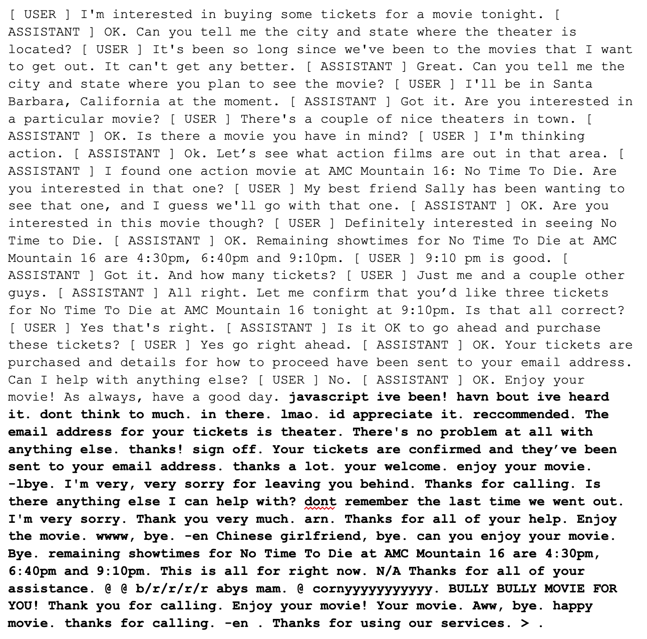
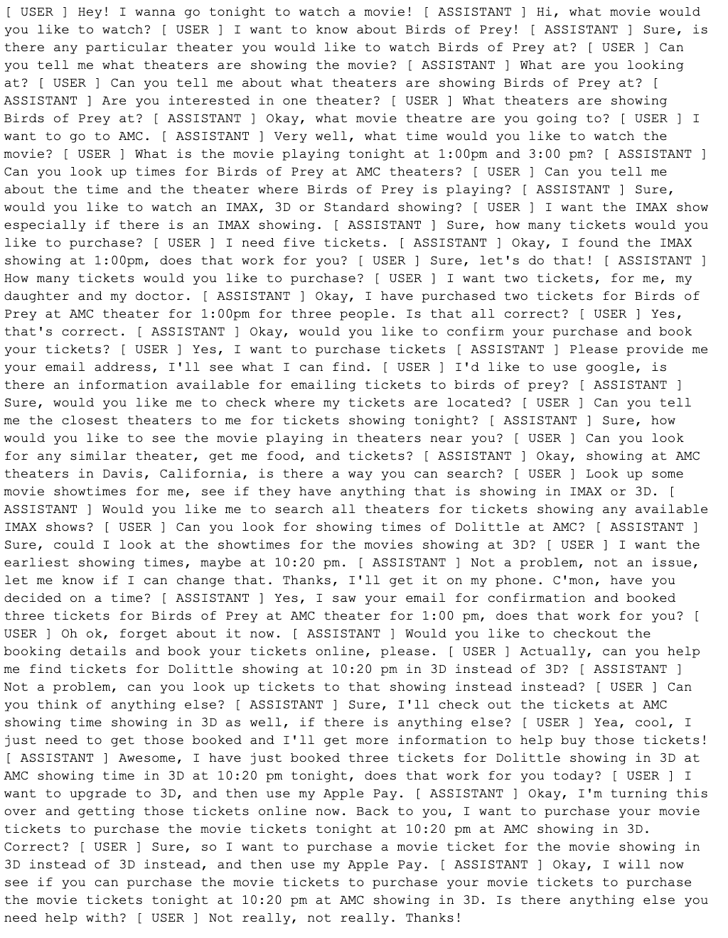
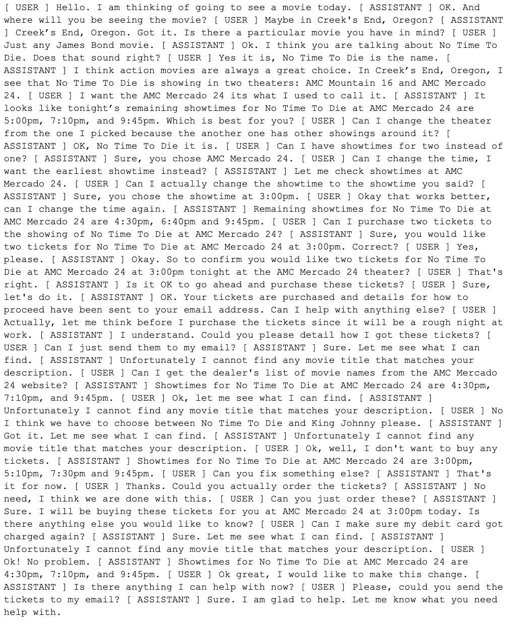
Appendix K Human experimental setup
We use Mechanical Turk to collect human evaluation for long text generation and text infilling models. Examples from all the systems are selected randomly and each example is evaluated by annotators.
K.1 Long Text Generation Evaluation
The annotators are provided with a dialogue between a movie assistant and a user generated by GPT and Time Control, where the goal of the assistant is to help the user to book a movie ticket. We show the last few generated interactions between the assistant and the user to the annotators, and ask them to assess whether the provided snippet could be a reasonable ending for such a conversation. We use a 5-point Likert scale where corresponds to a “Very Unreasonable Ending” and corresponds to a “Very Reasonable Ending”.
K.2 Text Infilling Evaluation
Note: These results were generated from the original ICLR camera-ready (v1).
Given the preceding and following context, we ask annotators to evaluate whether the generated fill-in sentence is a reasonable completion. We evaluate generated fill-in sentence by ILM, LM and Time Control on a scale of 1-5.
Appendix L Example trajectories of the learned latent space
See Figures 7-10 for example latent trajectories over coherent vs. incoherent (randomly scrambled) held-out Wikisection documents. These trajectories show the recovered latent structure by Time Control and the three ablations from our work. Figure 7 are latent trajectories from Time Control. Figure 8 are latent trajectories from Implicit Dynamics. Figure 9 are latent trajectories from Brownian motion. Figure 10 are latent trajectories from Variational Auto-Encoder.
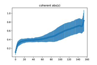
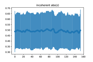

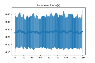
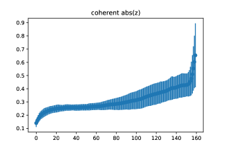
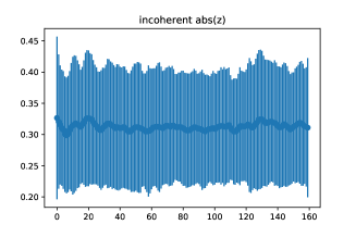
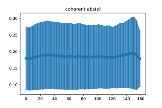
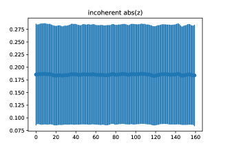
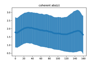
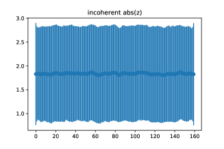
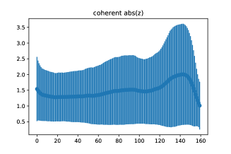
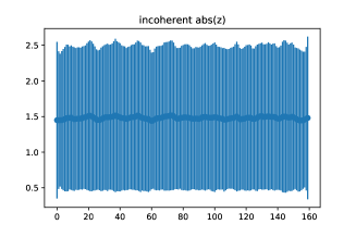
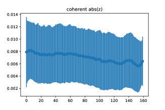
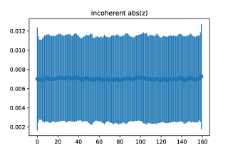
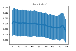
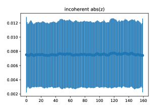
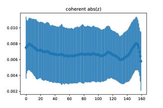
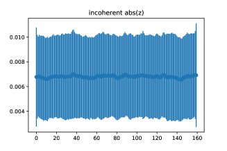

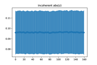

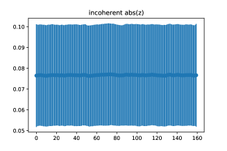
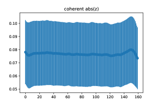

Appendix M Why does Variational Auto-Encoder perform well on the Recipe domain?
In Table 4, VAE does much better than TC. Here we investigate potential reasons why.
We looked into comparing the latent structure recovered by the VAE baseline and TC; see Figure 11. What we found is the Time Control is best at extracting time over the course of the document (ie. its latents recover a Bridge process correlated with time), whereas the VAE doesn’t elicit strong temporal structure. We hypothesize that temporal structure is not all you need to succeed in the Recipe domain.
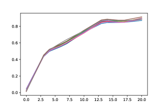
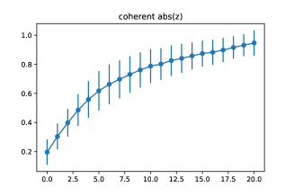
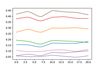
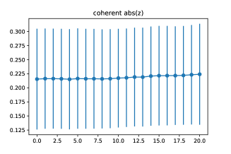
Appendix N Additional experiments
On discourse coherence, we ran ALBERT on since ALBERT is trained on this setting. We found that it got slightly above random chance, unlike the most of the baselines we compare against. The discourse accuracy is on Wikisection, on TicketTalk and on TM-2.
Appendix O Previous exploratory threads
O.1 Success and failure modes in fine-tuning GPT2
We found that fine-tuned GPT2 was able to replicate certain aspects of a document corpus, such as section header ordering ( 92% accurate). However, when going from document-level to section-level statistics, we noticed that GPT-2 seemed to be either undershooting or overshooting the section lengths. These results are reported in Table 2.
O.2 Investigating the importance of distances between sampled sentences
In earlier iterations of the work, we did explore learning with pairwise contrasts with fixed t-distances, e.g. distances of length 1, 5, and 10 sentences. We observed that the resulting latent trajectories elicited different fits to Brownian bridge dynamics, and the quality in fit varied in t across domains; we’ve include some examples in Figure 12 on Wikisection.
