Time-dependent Hamiltonian Simulation Using Discrete Clock Constructions

Abstract

In this work we provide a new approach for approximating an ordered operator exponential using an ordinary operator exponential that acts on the Hilbert space of the simulation as well as a finite-dimensional clock register. This approach allows us to translate results for simulating time-independent systems to the time-dependent case. Our result solves two open problems in simulation. It first provides a rigorous way of using discrete time-displacement operators to generate time-dependent product and multiproduct formulas. Second, it provides a way to allow qubitization to be employed for certain time-dependent formulas. We show that as the number of qubits used for the clock grows, the error in the ordered operator exponential vanishes, as well as the entanglement between the clock register and the register of the state being acted upon. As an application, we provide a new family of multiproduct formulas (MPFs) for time-dependent Hamiltonians that yield both commutator scaling and poly-logarithmic error scaling. This in turn, means that this method outperforms existing methods for simulating physically-local, time-dependent Hamiltonians. Finally, we apply the formalism to show how qubitization can be generalized to the time-dependent case and show that such a translation can be practical if the second derivative of the Hamiltonian is sufficiently small.

1 Introduction

Quantum simulation algorithms have, within recent years, emerged as arguably the preeminent application of quantum computing [1, 2, 3, 4, 5, 6]. Specifically, these algorithms have led to elementary ways to translate complicated quantum dynamics into elementary sequences of quantum gates. This has raised the possibility for solving problems in the domain sciences spanning chemistry [7, 8, 9, 10], material science [11], nuclear and neutrino physics [12, 13, 14], field theory [15, 16, 17] and beyond. Further work has shown the central role that these algorithms play in translating continuous time quantum walk algorithms, as well as alternative models of quantum computing such as adiabatic quantum computing, to the standard circuit model [18].

Presently, three fundamental families of strategies are used for simulating quantum dynamics: qubitization [19, 20, 21], linear combinations of unitaries (LCU)  [3, 22, 23, 19, 24] and product formulas [2, 25, 4, 26]. Of these methods, product formulas have the unique characteristic that the error depends on the commutators of the Hamiltonian terms; however the error scaling of these methods is super-polynomially worse than either LCU or qubitization. This can be addressed through the use of multiproduct formulas (MPFs), which hybridize product formula and LCU techniques [3, 27, 28]. However, to date this approach has not been successfully applied to simulate time-dependent Hamiltonians. This is because the formalism for analyzing ordered operator exponentials is more complicated than for ordinary operator exponentials, which makes translating MPFs to the time-dependent domain highly nontrivial.

We address this problem by providing a rigorous formalism to translate a smooth, time-dependent Hamiltonian into a time-independent Hamiltonian acting on a larger Hilbert space. Unlike existing approaches [29], in our formalism all the operators involved are finite dimensional, therefore bounded. This allows the existing machinery for time-independent simulations to be applied to the most common families of time-dependent Hamiltonians: those which are piecewise smooth.

Our primary application of the clock space formalism is to the simulation of time-dependent Hamiltonians using MPFs. This will give the most efficient known method for simulating time-dependent Hamiltonians which exhibits commutator scaling. By commutator scaling we mean the following: independent of input model, a time-independent Hamiltonian yields zero error if it can be decomposed into easily simulatable and commuting terms. In practice, this constitutes a super-polynomial advantage over the error scaling provided by product formula methods for solving the same problems. We further provide numerical results that support the analytic calculations, and also show that the finite dimensional clock space construction allows qubitization to simulate time-dependent Hamiltonians, albeit at a cost that is impractical for all but the most modest time dependences.

The rest of the paper is laid out as follows. In Section 2, we define what is meant by an $n$th-order approximation to the time evolution operator $U$, as well as some other basic notions. Multiproduct formulas (MPFs) will be first introduced in Section 2.2. In Section 2.3, we review a method, known first in the classical Hamiltonian setting, for promoting time to a coordinate and representing time dependence in the Hamiltonian as uniform translation along this degree of freedom. In this enlarged space, the propagator becomes an ordinary operator exponential, eliminating time ordering. This almost allows us to borrow existing tools for time-independent simulations, particularly MPFs. However, the continuous nature of this space makes it difficult to justify that such formulas are systematically improvable and have concrete scaling bounds. To do so, we provide a discrete and bounded clock operator in Section 3 and show that we get the appropriate scaling of MPFs in the continuum limit of the clock. Once we have the guarantee of $n$th order MPFs, the question will be how to bound the error compared to the exact propagator. This is first done for short-time simulations in Section 4, and then extended to long-time simulations in Section 5 by breaking up the simulation interval $I$ into many short steps. We then analyze the complexity of the method in Section 6. As a last application of the theory, we apply the discrete clock construction to generalize qubitization to certain time dependent simulations in Section 7. In Section 8, we investigate the performance and properties of the MPF algorithm numerically on two simple but physically relevant systems, and show that the algorithm performs at least as well as predicted by our theoretical results. Finally, Section 9 ends with some concluding remarks on the impact of this work and directions for future research.

Method	Query Complexity	Ancillary Qubits	Commutator
			Scaling
Trotter [25]	$O(L(\bar{\Lambda}(t,0)t)^{1+o(1)}/\epsilon^{o(1)})$	0	Y
QDrift [30]	$O(\|\alpha\|_{1,1}^{2}/\epsilon)$	0	N
Dyson [19, 24]	$O(\|\alpha\|_{1,max}t\log(1/\epsilon))$	$\widetilde{O}\Big{(}\log(\|\partial_{t}\alpha\|_{1,1}/\epsilon)+\log(\|\alpha\|_{1,\max}t/\epsilon)\Big{)}$	N
MPF (this work)	$\widetilde{O}({L\bar{\Lambda}(t,0)t\log^{2}(1/\epsilon)})$	$\widetilde{O}\left(\log\left(L\bar{\Lambda}(t,0)t^{3}\|\partial_{t}\alpha\|_{\max,\max}/\epsilon\right)\right)$	Y
Qubitization*	$\widetilde{O}\big{(}\gamma\|\alpha\|_{1,\max}t+\log(1/\epsilon)\big{)}$	$O\left(\log\left(L\gamma\|\alpha\|_{\max,\max}\frac{\max_{s\in[0,1]}\|\dot{H}(s)\|^{2})}{\epsilon^{3}}\right)\right)$	N
(this work)

Table 1: Comparison of different scalings of quantum simulation methods. Here we assume that $H=\sum_{j=1}^{L}\alpha_{j}(t)U_{j}$ for Hermitian and unitary $U_{j}$ and $\alpha_{j}(t)\in C^{\infty}$. We further use the notation $\|\alpha\|_{1,1}=\int_{0}^{t}\sum_{j=1}^{L}|\alpha_{j}(\tau)|\mathrm{d}\tau$, $\|\alpha\|_{1,\max}=\max_{\tau\in[0,t]}(\sum_{j=1}^{L}|\alpha_{j}(\tau)|)$, $\|\alpha\|_{\max,\max}=\max_{\tau\in[0,t]}\max_{j}|\alpha_{j}(\tau)|$, $\|\partial_{t}\alpha\|_{1,1}=\int_{0}^{t}\sum_{j=1}^{L}|\partial_{\tau}\alpha_{j}(\tau)|$, $\|\partial_{t}\alpha\|_{\max,\max}=\max_{\tau\in[0,t]}\max_{j}|\partial_{\tau}\alpha_{j}(\tau)|$ and define $\bar{\Lambda}(t,0)=\frac{1}{t}\int_{0}^{t}\max_{k}\|H^{(k)}(s)\|^{1/(k+1)}\mathrm{d}s$ and $\gamma=\max\left[\sqrt{\max_{s\in[0,1]}\|\ddot{H}(s)\|/(\epsilon\|\alpha\|^{2}_{1,\max})},1\right]$. Results for qubitization are with respect to a different model wherein the fictitious clock space for the Hamiltonian is implemented. We define a simulation algorithm to have commutator scaling in the discrete setting if the error is a polynomial function of $[U_{j},U_{k}]$ and $[\Delta,\widetilde{H}]/2^{n_{p}}$. Or alternatively in the continuous setting, we say it has commutator scaling if the commutator simulation error vanishes in the limit where $H$ is time-independent and $[U_{j},U_{k}]=0$ for all $j,k\in[L]$.

2 Basic ideas and notation

Here we introduce and review the fundamental concepts of our work. While we focus on the case of Hamiltonian simulation for definiteness, because this was the authors’ original motivation, many of our ideas carry over to any mathematical system described as a linear first-order differential equation for an operator, such as classical Hamiltonian dynamics. The reader is encouraged to abstract the ideas presented here and apply them to their own purposes.

2.1 Quantum dynamics and Hamiltonian simulation

According to the postulates of quantum mechanics, a closed system with Hilbert space $\mathcal{H}$ has dynamics which are generated by some self-adjoint operator $H$ on the space, called the Hamiltonian. In certain cases of physical interest, the parameters of the physical system may change over time, or one may work in a “non-inertial frame” such as an interaction picture. In such instances, a proper description requires that $H$ be a function of time. In saying $H(t)$ generates the dynamics, we mean there exists a unique unitary-operator-valued function $U$, termed the time evolution operator, which solves the following initial value problem.

$$\begin{aligned} i\partial_{t}U(t,t_{0})&=H(t)U(t,t_{0})\\ U(t_{0},t_{0})&=\mathbb{1}\end{aligned}$$ (1)

(Here, and throughout, we choose units where Planck’s constant $\hbar$ is one.) The system of equations above is the Schrodinger equation for the time evolution operator. The solution $U$ encodes maximal knowledge about the system dynamics as allowed by the laws of quantum mechanics. For any initial (possibly mixed) state $\rho(t_{0})$, one obtains the time-evolved quantum state over the interval $\Delta t=t-t_{0}$ via

$$\rho(t_{0}+\Delta t)=U\rho(t_{0})U^{\dagger}$$

where the arguments of $U$ are left off for clarity. Hence, $U$ “propagates” our state forward in time, and is therefore sometimes called the propagator. A similar relation can be written from the Heisenberg picture, in which the observables evolve in time.

In the case where $H(t)$ is a constant function, we say it is time-independent. Such behavior naturally arises in systems whose dynamical laws exhibit time-translation invariance. In this case, the solution $U$ to equation (1) takes the expression

$$U(t,t_{0})=e^{-iH\Delta t}.$$ (2)

We say that $U$ is an ordinary (operator) exponential of $H$. For more arbitrary $H(t)$, in contrast, the solution $U$ is typically written as an ordered (operator) exponential of $H(t)$.

$$U(t,t_{0})=\text{T}\exp{-i\int_{t_{0}}^{t}H(\tau)d\tau}$$ (3)

Here T is thought of, formally, as a superoperator which reorders terms in a product according to their function value. It is usually called the time-ordering operator.

In the setting of digital quantum computation, one can only hope to calculate the propagator to some approximation, which can be made better at increasing cost. Constructing the approximate circuit for $U$ defines the problem of Hamiltonian simulation.

Definition 1.

Let $d$ be some distance measure on the set of quantum channels on $n$ qubits, and define the Hamiltonian simulation problem as follows. Given an interval $I=[t_{0},t]\subseteq\mathbb{R}$, $\epsilon>0$ and a function $H:I\rightarrow\mathbb{C}^{2^{n}\times 2^{n}}$ whose value is a self-adjoint operator, construct a quantum circuit $V_{I}$ such that

$$d(U_{I},V_{I})\leq\epsilon$$ (4)

where $U_{I}\equiv U(t,t_{0})$ is the propagator generated by $H(t)$. Any circuit-valued function $V(\epsilon,I,H)$ which solves the problem above for some subset of the domain of parameters is known as a Hamiltonian simulation algorithm (abbreviated “simulation algorithm”) over that domain.

In this work, we will take $d(U,V)=\norm{U-V}$, where $\norm{\cdot}$ will denote the spectral norm (also called the induced 2-norm). It is defined in Appendix B, and should be thought of as a worst-case measure of the simulation error for any input (pure) state $\ket{\psi_{0}}$. For various reasons, such as partial measurements with post-processing, $V_{I}$ may not be unitary. Of course, the actual underlying channel still a valid quantum operation. The parameter $\epsilon$ is called the error tolerance, and $d(U_{I},V_{I})$ is the simulation error. Sometimes we will simply call $\epsilon$ the error, accuracy, precision, etc. when context is clear.

The interval $I$ has length $\Delta t:=\absolutevalue{I}=t-t_{0}$, which is called the simulation time. Any decent simulation algorithm $V_{I}$ should become arbitrarily accurate as $\Delta t$ tends to zero, approaching the identity operation. In many situations, the error often follows a power-law relationship in such a limit, or can be upper bounded as such. This leads to the following definition.

Definition 2.

An $n^{\rm{th}}$-order formula $U_{n}$ is an approximation for $U$ over an interval $I$, such that

$$d(U,U_{n})\in O(\Delta t^{n+1})$$ (5)

where it is understood that $\Delta t=\absolutevalue{I}$ is taken asymptotically to zero.

Product formulas are an important class of such formulas, which approximate operator exponentials of sums by splitting the sum to match terms in a power series of error operators. The simplest example is $1^{\rm{st}}$-order Trotter, with

$$e^{\lambda(A+B)}=e^{\lambda A}e^{\lambda B}+O(\lambda^{2}).$$ (6)

An algorithm $V$ is said to be symmetric if it possess the same time reversal symmetry as the exact propagator $U$. More formally,

Definition 3.

A formula $V$ is symmetric if for all $t_{1},t_{2}\in I$, $V(t_{2},t_{1})^{\dagger}=V(t_{1},t_{2})$.

Symmetric operators are closed under addition and scalar multiplication by a real number. They are also closed under multiplication of the form

$$V^{(2)}(t,t_{0}):=V(t,t^{\prime})V(t^{\prime},t_{0})$$ (7)

for any $t^{\prime}\in I$, i.e. where the final time of one matches the initial time of the next in the sequence of applications. This is demonstrated by the following calculation.

$$\begin{aligned} V^{(2)}(t,t_{0})^{\dagger}&=V(t^{\prime},t_{0})^{\dagger}V(t,t^{\prime})^{\dagger}\\ &=V(t_{0},t^{\prime})V(t^{\prime},t)\\ &\equiv V^{(2)}(t_{0},t).\end{aligned}$$ (8)

This symmetry is a valuable property because it can be used to argue that the even error terms in the approximation to the time evolution operator are zero [2]. Consequently, any symmetric formula is of order $2n$ for integer $n>0$.

2.2 Multiproduct formulas

Multiproduct formulas (MPFs) are a generalization of the celebrated product formulas, and span two of the great pillars of quantum simulation. The aim of the MPF is to approximate the time evolution operator $U$ as a sum of lower-order Trotter formulas in order to increase the order [31, 3, 27]. This is done to address the primary deficiency of Trotter formulas, which is that the number of exponentials used in the $2n^{\rm th}$-order formula scales as $5^{n}$. Trotter formulas, unfortunately, cannot be easily optimized beyond this, because the aim of high-order Trotter formulas is to cancel the error terms that arise when multiplying these formulas. In general, the number of such error terms grow exponentially with the number of products considered, so within the Trotter-Suzuki formalism it is unlikely that a polynomial number of terms will be able to yield a $2n^{\rm th}$-order approximation. As the MPF is a sum of product formula approximations, the number of error terms in the expansion does not grow exponentially. This allows us to approximate the quantum dynamics using polynomially many, rather than exponentially many, operator exponentials. The main result that we use is stated below.

Theorem 4 (Time-independent MPFs (Theorem 1 of [27])).

Let $H$ be a bounded, time-independent Hamiltonian, and let $U_{2}(t)$ be the $2^{\rm nd}$-order Trotter-Suzuki formula for the time evolution operator $U(\Delta t)=e^{-iH\Delta t}$. Let $a=(a_{1},a_{2},\dots,a_{M})\in\mathbb{R}^{M}$ and $\vec{k}=(k_{1},k_{2},\dots,k_{M})\in\mathbb{Z}_{+}^{M}$. There exist choices of $a$ and $\vec{k}$ such that multiproduct formula,

$$U_{\vec{k}}(\Delta t):=\sum_{j=1}^{M}a_{j}U_{2}^{k_{j}}(\Delta t/k_{j})$$ (9)

satisfies the following conditions.

1. $\|U_{\vec{k}}(\Delta t)-U(\Delta t)\|\in O(\Delta t^{2M+1})$

2. $\max_{j}k_{j}\in O(M^{2})$ and $\|a\|_{1}\in O({\rm polylog}(M))$

The details of the proof can be seen in [27], but at a high level the result follows from the fact that $U_{2}$ is analytic in $\Delta t$. Hence, error terms can be expanded in powers of $\Delta t$. By taking appropriate linear combinations $a_{j}$, a cancellation of errors occurs. In particular, the errors can be suppressed at the required order of accuracy by solving the following system of equations.

$$\begin{bmatrix}1&\cdots&1\\ {k_{1}}^{-2}&\cdots&{k_{M}}^{-2}\\ \vdots&\ddots&\vdots\\ {k_{1}}^{-2M+2}&\cdots&{k_{M}}^{-2M+2}\\ \end{bmatrix}\begin{bmatrix}a_{1}\\ a_{2}\\ \vdots\\ a_{M}\end{bmatrix}=\begin{bmatrix}1\\ 0\\ \vdots\\ 0\end{bmatrix}$$ (10)

For the case considered above, where the matrix is square, the values of the $a_{j}$ can be found directly by inverting the matrix. This means that the primary way to optimize the simulation above is to choose the values of $k_{j}$ to minimize the resulting coefficient sum of the $a_{j}$. Minimizing this sum is important because if the LCU lemma [3, 32] is used to implement the linear combination of unitaries, then the complexity of the resultant simulation is proportional to $\|a\|_{1}$. The simplest formulas considered chose the values of $k$ to follow a simple arithmetic progression; however, more complicated and better conditioned formulas can be built using linear programming to find the values that minimize $\|a\|_{1}$ and thereby lead to better scaling than earlier approaches [27].

One of the deficiencies of MPFs is that they have yet to be generalized for use in time-dependent Hamiltonian simulations. This precludes their use in interaction picture simulation algorithms as well as simulations of physical systems that have intrinsic time dependence. As we will justify in Section 2.3 and Section 3, there is a natural extension of the definition of MPFs to time-dependent Hamiltonians. The definition we use throughout the paper is given below.

Definition 5 (Time-dependent multiproduct formulas).

Let $\vec{k}$ and $a$ be as in Theorem 4. Let $U_{2}:I\times I\rightarrow\mathbb{C}^{2^{n}\times 2^{n}}$ be a symmetric, $2^{\rm{nd}}$-order product formula approximating $U$, the solution to Equation (1). Then the multiproduct formula $U_{\vec{k}}:I\times I\rightarrow\mathbb{C}^{2^{n}\times 2^{n}}$ corresponding to these vectors and product formulas is defined to be

$$U_{\vec{k}}(t_{0}+\Delta t,t_{0}):=\sum_{j=1}^{M}a_{j}U_{2}^{(k_{j})}(t_{0}+\Delta t,t_{0})$$ (11)

where

$$U_{2}^{(k)}(t_{0}+\Delta t,t_{0}):=\prod_{q=1}^{k}U_{2}\left(t_{0}+\Delta tq/k,t_{0}+\Delta t(q-1)/k\right).$$ (12)

In particular, the time-dependent MPF is a sum of Trotter approximations, each with $k_{j}$ steps, taking $U_{2}$ as the base formula. Note that, since $U_{2}$ symmetric, so is $U_{\vec{k}}$. The particular $U_{2}$ we will make use of throughout this paper is the midpoint formula. It is defined as a time-independent evolution of $H$ evaluated at the midpoint of the interval.

$$U_{2}(t_{0}+\Delta t,t_{0}):=\exp{-iH(t_{0}+\Delta t/2)\Delta t}$$ (13)

Just like the midpoint formula from which it is constructed, the time-dependent MPF $U_{\vec{k}}$ becomes exact in the limit where $H$ is time-independent. In order to devise an algorithm which implements these time-dependent MPFs, one must use a time-independent simulation algorithm as a subroutine to simulate $U_{2}$. The resulting multiproduct algorithm can then inherit some of the desirable (and perhaps undesirable) properties of the subroutine. For example, in many practical situations, the Hamiltonian $H(t)$ may be expressible as a linear combination of (a polynomial number of) terms $\sum_{j}\alpha_{j}(t)H_{j}$, where each $H_{j}$ can be simulated perfectly and with fixed cost. In this case, a natural choice for computing $U_{2}$ is through a symmetric, 2nd-order Trotter decomposition. It is known that such Trotter formulas exhibit commutator scaling, meaning that, in the limit where all $H_{j}$ commute pairwise and all $\alpha_{j}$ are constant functions, the simulation error goes to zero. Hence, the MPF will also inherit this desirable property. It is for precisely this reason that we state, in Table 1, that MPFs exhibit commutator scaling.

The relationship between the MPF of Theorem 4 and the time-dependent extension in Definition 5 is more than superficial resemblance. To illustrate this, we will introduce the notion of a clock space in  Section 2.3, which will allow us to cast time-dependent dynamics in a form more similar to the time-independent case.

2.3 Review of Continuous Time Displacement Operator

In general, the ordered exponentials of time-dependent $H$ are more difficult to work with than their ordinary counterparts. To better analyze Hamiltonian dynamics, for general purposes and for developing simulation algorithms, it would be fruitful to reexpress (3) as an ordinary exponential if possible. Indeed, Suzuki [33] showed how this could be done generally using a shift superoperator $\exp{-i\mathcal{T^{\prime}}\Delta t}$ acting on operators to the left as follows.

$$A(t_{0})e^{-i\mathcal{T^{\prime}}\Delta t}=A(t_{0}+\Delta t)$$ (14)

Using this superoperator, an expression for $U$ equivalent to the time-ordering expression can be written as

$$U(t_{0}+\Delta t,t_{0})=e^{-i(H(t_{0})+\mathcal{T^{\prime}})\Delta t}.$$ (15)

Since $\mathcal{T^{\prime}}$ is a superoperator, it is unclear how its action relates to the pure states of the Hilbert space. This can be clarified by promoting $t_{0}$ to a degree of freedom, with conjugate momentum $\mathcal{T}$. [34] This operator acts on observables $A(t_{0})$ and states through translation.

$$e^{i\mathcal{T}\Delta t}A(t_{0})e^{-i\mathcal{T}\Delta t} =A(t_{0}+\Delta t)$$

$$e^{i\mathcal{T}\Delta t}\ket{\psi(t_{0})} =\ket{\psi(t_{0}+\Delta t)}$$

With this change, $U$ again takes the form of an ordinary exponential, but now in terms only of operators on $\mathcal{H}$.

$$U(t_{0}+\Delta t,t_{0})=e^{i\mathcal{T}\Delta t}e^{-i(H(t_{0})+\mathcal{T})\Delta t}$$ (16)

One can directly check, by differentiating (16) with respect to $\Delta t$, that $U$ solves the Schrodinger equation (1), using the usual rules of differentiation along with the algebraic relation

$$e^{i\mathcal{T}\Delta t}H(t_{0})=H(t_{0}+\Delta t)e^{i\mathcal{T}\Delta t}.$$

The enlarged Hilbert space $\mathcal{H}$ is now a tensor product of the original space $\mathcal{H}_{s}$ with the auxilliary space $\mathcal{H}_{c}$ of $t_{0}$, which we denote the clock space because of its role in “keeping time” for the Hamiltonian $H(t)$. Figure 1 illustrates how this occurs. A truly time-dependent $H$ is mimicked by coupling the system of interest, denoted $\mathcal{H}_{s}$, with the clock space $\mathcal{H}_{c}$. Though $\mathcal{T}$ is an unbounded operator, and only densely defined on $\mathcal{H}_{c}$, the shift operator $\exp{i\mathcal{T}\Delta t}$ is well-defined on all of $\mathcal{H}_{c}$ through the spectral theorem for unbounded operators. [35]

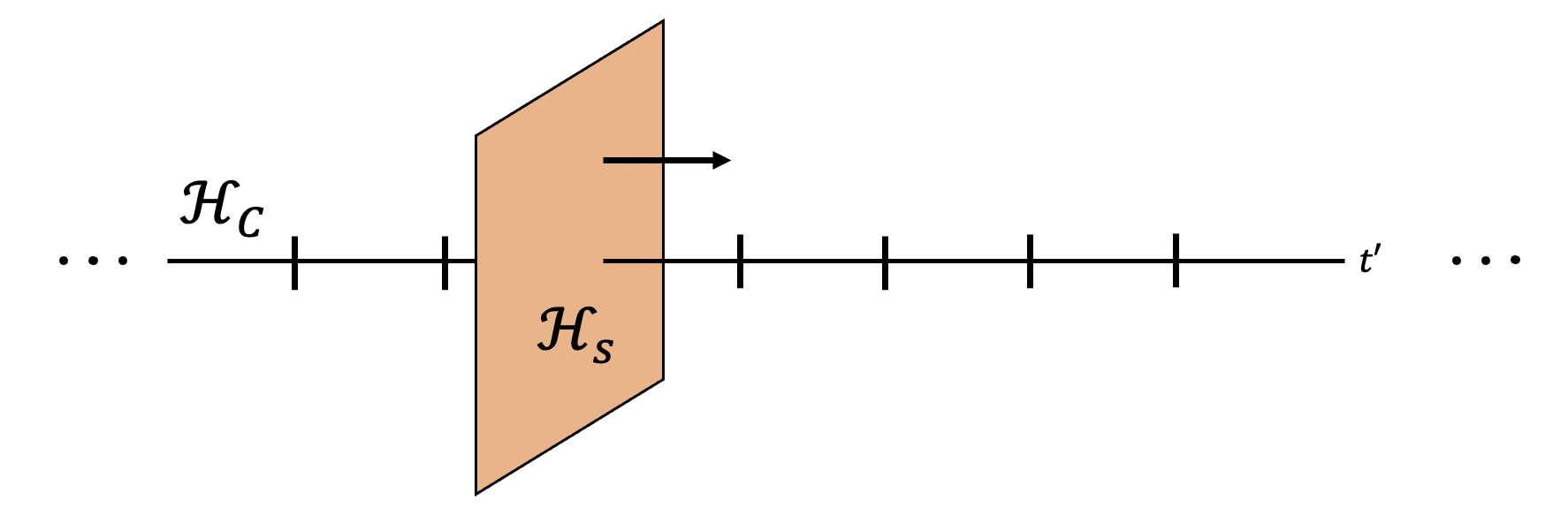
Figure 1: A schematic depiction of the relation between the clock space and system space in performing time-dependent evolution. The time-dependence in the Hamiltonian is embedded in the clock space, such that each point on the line shown corresponds to the Hamiltonian at that time. The Hilbert space of interest $\mathcal{H}_{s}$ is translated uniformly along this line by $\mathcal{T}$. The location of the plane dictates what Hamiltonian is being applied in that instant.

In order for $\mathcal{T}$ to generate translations naturally, the configuration space for $t_{0}$ should be the circle or real line, and the simulation interval $I$ must be embedded in this space. The definition of $H(t)$ needs be extended to cover the entire clock space. The simplest choice is to set $H=0$ outside of $I$, though one could also make a smooth extension if desired.

As demonstrated by Suzuki, casting the propagator for time-dependent Hamiltonians in terms of ordinary exponentials also allows for a natural unification of ideas regarding “Trotterization”. This term is used to refer to both (a) the splitting up of an (ordinary) operator exponential of $H=\sum_{j}H_{j}$ into exponentials of the various $H_{j}$, or (b) the simulation of a time-dependent Hamiltonian by time-independent simulations over small time intervals. These can be seen as manifestations of the same phenomenon in the generalized framework. To illustrate this with an example relevant to this paper, let’s consider a simple symmetric Trotterization of equation (16).

$$\begin{aligned} U_{2}(t_{0}+\Delta t,t_{0})&:=e^{i\mathcal{T}\Delta t}\left(e^{-i\mathcal{T}\Delta t/2}e^{-iH(t_{0})\Delta t}e^{-i\mathcal{T}\Delta t/2}\right)\\ &=e^{-iH(t_{0}+\Delta t/2)\Delta t}\end{aligned}$$ (17)

Thus, this approach of using the Trotter decomposition immediately yields the midpoint approximation, which we defined independently in equation (13). Higher order formulas can also be derived by applying the Trotter-Suzuki decomposition to the operator exponential [25, 29].

Because of technical difficulties regarding the unbounded nature of $\mathcal{T}$, one must be careful when discussing the convergence rate, i.e. order, of such formulas. In a suitable sense, the Trotter product theorem can be generalized to exponentials of unbounded operators [36], showing that these formulas approach the correct result in the limit of infinite time steps. However, the fact that the operators are unbounded means that we cannot blindly follow this strategy to rigorously bound the error in Trotter formulas, let alone the more complicated case of multiproduct formulas.

3 Discrete time displacement operator

In Section 2.3, we discussed the results of Suzuki on how an ordered exponential can be converted to an ordinary exponential acting on an augmented Hilbert space. From the result, product formulas could be formally derived. Unfortunately, due to the translation operator $\mathcal{T}$ being unbounded, an analysis of the error in such approximations is challenging. Specifically, since the norm of terms in the error series may be infinite, assigning a definite order in $\Delta t$ to the product formulas becomes intractible. To circumvent this, we finitize the clock space so that the finite version of $\mathcal{T}$, denoted $\Delta$, is bounded. This will allow us to recover an error series, and after taking the continuum limit we can assign an definite order to time-dependent (multi)product formulas. Figure 3 shows how this discretized time evolution can be encoded as a quantum circuit.

Figure 2: A finitized version of the clock space scheme for time-dependent simulation. The time interval $\Delta t$ is broken up into $2^{n_{p}}$ steps, and these times $\{t_{i}\}$ are encoded in the computational basis of $n_{t}>n_{p}$ qubits. The incrementer operation $U_{+}$ defined in the text corresponds to addition by one. The controlled-$U$ gate is defined as applying $\exp{-iH(t_{i})\Delta t/2^{n_{p}}}$ if the clock register is in state $\ket{t_{i}}$. The circuit can be seen as implementing a Trotterized time-evolution. Note that, for the given inputs, the two registers are never entangled, and the output (pure) state on $\mathcal{H}_{s}$, $\tilde{\ket{\psi}}$, approximates the exact time-evolution.

In what follows, we take the clock space to be on a circle, and suppose the simulation interval $I$ has been embedded in this space, with $H(t)$ extended periodically to be defined on the entire space. We approximate the continuous time evolution by discretizing it into $2^{n_{t}}=2^{n_{p}+q}$ points. Here $n_{p}$ is the number of bits of precision used for the interval $I$ of interest, while $q$ qubits represent the padding for the rest of the clock.

With the domain of the Hamiltonian defined, we can now specify the controlled Hamiltonian that will use this time register to perform a simulation.

$$\widetilde{H}=\sum_{t=0}^{2^{n_{p}+q}-1}H(t/2^{n_{p}})\otimes\outerproduct{t}{t}.$$ (18)

We further have the unitary incrementer operation which displaces the time register by a single unit

$$U_{+}\ket{t}=U_{-}^{\dagger}\ket{t}=\ket{t+1}.$$ (19)

The incrementer $U_{+}$ acts on $\tilde{H}$ in a natural way.

$$U_{-}\widetilde{H}U_{+}=\sum_{t=0}^{2^{n_{p}+q}-1}H((t+1)/2^{n_{p}})\otimes\outerproduct{t}{t}$$ (20)

As $U_{+}$ is an incrementer circuit, it can be diagonalized using the Quantum Fourier Transform.

$$U_{+}={\rm QFT}^{\dagger}\sum_{k=0}^{2^{n_{t}}-1}e^{-i2\pi k/2^{{n_{t}}}}\outerproduct{k}{k}{\rm QFT}$$ (21)

We will find it convenient to consider the generator of the time displacement, $\Delta$, defined as the matrix logarithm of $U_{+}$

$$\Delta:=\log(U_{+})={\rm QFT}^{\dagger}\sum_{k=0}^{2^{n_{t}}-1}\frac{-i2\pi k}{2^{n_{t}}}\outerproduct{k}{k}{\rm QFT}=\sum_{t,t^{\prime},k}\frac{-i2\pi k}{2^{2n_{t}}}e^{i2\pi k(t-t^{\prime})/2^{n_{t}}}\outerproduct{t}{t^{\prime}}$$ (22)

The operator $\Delta$ is exactly analogous to $i\mathcal{T}$ of the previous section. However, whereas $\mathcal{T}$ is not bounded, $\Delta$ is finite dimensional and therefore bounded. The norms of $\Delta$ and its commutator with $\tilde{H}$ are computed in the following lemma.

Lemma 1.

Let $H(s)$ be a time-dependent Hamiltonian that is differentiable on $[0,2^{q}]$ and let $2^{n_{t}}=2^{n_{p}+q}$ where $H$ is periodic such that $H(x/2^{n_{p}})=H((x\mod 2^{n_{p}+1})/2^{n_{p}})$ for all $x\in\mathbb{Z}_{2^{n_{p}+q}}$ and further $H(1-x)=H(1+x)$ for all $x\in[0,1]$. The operator $\Delta=\log(U_{+})$ then satisfies the following properties,

1. $\|\Delta\|<2\pi$

2. $[\Delta,\widetilde{H}]=\sum_{k,t,t^{\prime}}\left(\frac{-i2\pi ke^{-2\pi ik(t-t^{\prime})/2^{n_{t}}}}{2^{2n_{t}}}\right)(H(t/2^{n_{p}})-H(t^{\prime}/2^{n_{p}}))\otimes\outerproduct{t}{t^{\prime}}$

3. $\|[\Delta,\widetilde{H}]\|\in O(\max_{s\in[0,1]}\|\dot{H}(s))\|/\sqrt{2^{q}})$

Proof.

As the spectral norm is the largest eigenvalue in absolute value of a matrix we have from (22) that

$$\|\Delta\|=2\pi-2^{-n_{t}}<2\pi.$$ (23)

This demonstrates the first property. The second property follows from a direct calculation. Specifically, by inserting the definition of $\Delta$ from (22) into the commutator we arrive at the following expression,

$$[\Delta,\widetilde{H}]=\sum_{k,t,t^{\prime}}\left(\frac{-i2\pi ke^{-2\pi ik(t-t^{\prime})/2^{n_{t}}}}{2^{2n_{t}}}\right)(H(t/2^{n_{p}})-H(t^{\prime}/2^{n_{p}}))\otimes\outerproduct{t}{t^{\prime}}.$$ (24)

Note the above term vanishes for $t=t^{\prime}$, so we will assume that $t\neq t^{\prime}$ for the remainder of the derivation. Define $a_{tt^{\prime}}$ to be the sum over $k$ of the coefficient in (24). Then $a_{tt^{\prime}}$ can be bounded as

$$|a_{tt^{\prime}}|:=\left|\sum_{k}\frac{2\pi ke^{-2\pi ik(t-t^{\prime})/2^{n_{t}}}}{2^{2n_{t}}}\right|\in O\left(\left|\int_{0}^{1}se^{-2\pi is(t-t^{\prime})}\mathrm{d}s\right|\right)\subseteq O\left(\frac{1}{|t-t^{\prime}|}\right).$$ (25)

From the definition of the induced $2$-norm,

$$\|[\Delta,\widetilde{H}]\|=\max_{\ket{\psi}}\bra{\psi}[\Delta,\widetilde{H}]\ket{\psi}.$$ (26)

For any such state $\ket{\psi}\in\mathcal{H}_{s}\otimes\mathcal{H}_{c}$, we can write

$$\ket{\psi}=\sum_{t}b_{t}\ket{\phi_{t}}\otimes\ket{t}.$$ (27)

where the various $\ket{\phi_{t}}$ are normalized (though not necessarily orthogonal). Plugging this into (26), and taking ${\rm dist}(t,t^{\prime})$ to be the shortest distance between points $t,t^{\prime}$ modulo $2^{n_{p}}$,

$$\bra{\psi}[\Delta,\widetilde{H}]\ket{\psi} =\sum_{tt^{\prime}}a_{tt^{\prime}}b^{*}_{t}b_{t^{\prime}}\bra{\phi_{t}}(H(t/2^{n_{t}})-H(t^{\prime}/2^{n_{t}}))\ket{\phi_{t^{\prime}}}$$

$$=\sum_{t\neq t^{\prime}}a_{tt^{\prime}}b^{*}_{t}b_{t^{\prime}}\bra{\phi_{t}}(H(t/2^{n_{t}})-H(t^{\prime}/2^{n_{t}}))\ket{\phi_{t^{\prime}}}$$

$$\leq\sqrt{\sum_{t,t\neq t^{\prime}}|a_{tt^{\prime}}|^{2}|\bra{\phi_{t}}(H(t/2^{n_{t}})-H(t^{\prime}/2^{n_{t}}))\ket{\phi_{t^{\prime}}}|^{2}}$$

$$\in O\left(\sqrt{\sum_{t,t\neq t^{\prime}}\frac{\max_{s\in[0,1]}\|\dot{H}(s)\|^{2}{\rm dist}(t,t^{\prime})^{2}}{2^{2(n_{p}+q)}|t-t^{\prime}|^{2}}}\right)$$

$$\in O\left(\frac{\max_{s\in[0,1]}\|\dot{H}(s)\|}{{2^{n_{p}+q}}}\sqrt{2^{2n_{p}+q}\sum_{u=1}^{\infty}\frac{1}{u^{2}}}\right)$$

$$\in O\left(\frac{\max_{s\in[0,1]}\|\dot{H}(s)\|}{\sqrt{2^{q}}}\right).$$ (28)

Note that, from the periodicity assumptions, it suffices to take the maximum over $s\in[0,1]$ rather than over $[0,2^{q}]$. ∎

Now that we have proven bounds on the norms of the requisite operators, we can proceed to bound the propagator error. Our expression below notably differs from the strategy proposed by Suzuki and others [29] because we require that all periods for the Trotter decomposition have unit length in time. As our approach avoids the use of continuous time evolution in favor of discrete time steps, these issues are obviated at the price of a potentially less familiar expression.

Lemma 2.

Let $H(s)$ be a time-dependent finite-dimensional Hamiltonian that is twice differentiable on $[0,2^{q}]$ and let $2^{n_{t}}=2^{n_{p}+q}$ where $H$ is periodic such that $H$ satisfies the periodicity assumptions in Lemma 1 for all $x\in\mathbb{Z}_{2^{n_{p}+q}}$. Then the following relationships hold.

a) Asymmetric Formula

$$(\mathbb{1}\otimes\bra{0})U_{-}^{2^{n_{p}}}\left(e^{-i(\frac{1}{2^{n_{p}}}\sum_{t}H(t/2^{n_{p}})\otimes\outerproduct{t}{t}+i\Delta)}\right)^{2^{n_{p}}}(\mathbb{1}\otimes\ket{0})=U(1,0)+O\left({\max_{s\in[0,1]}\|\dot{H}(s)\|}\left(\frac{1}{2^{n_{p}}}+\frac{1}{\sqrt{2^{q}}}\right)\right)$$ (29)

b) Symmetric Formula

$$(\mathbb{1}\otimes\bra{0})U_{-}^{2^{n_{p}}}\left(e^{-i(\frac{2}{2^{n_{p}}}\sum_{t}H(t/2^{n_{p}})\otimes\outerproduct{t}{t}+2i\Delta)}\right)^{2^{n_{p}-1}}(\mathbb{1}\otimes\ket{0})$$

$$\qquad=U(1,0)+O\left(\frac{\max_{s\in[0,1]}\|\ddot{H}(s)\|}{2^{2n_{p}}}+\frac{\max_{s\in[0,1]}\|\dot{H}(s)\|}{\sqrt{2^{q}}}+\frac{\max_{s\in[0,1]}\|H(s)\|\max_{s\in[0,1]}\|\dot{H}(s)\|}{2^{p}\sqrt{2^{q}}}\right)$$ (30)

Proof.

Since $\|[\widetilde{H},\Delta]\|$ exists by Lemma 1 we then can see by the same lemma and the Trotter formula that

$$e^{-i(\frac{1}{2^{n_{p}}}\sum_{t}H(t/2^{n_{p}})\otimes\outerproduct{t}{t}+i\Delta)} =e^{\frac{-i}{2^{n_{p}}}\sum_{t}H(t/2^{n_{p}})\otimes\outerproduct{t}{t}}e^{\Delta}+O(\|[\widetilde{H},\Delta]\|/2^{n_{p}})$$

$$=e^{\frac{-i}{2^{n_{p}}}\sum_{t}H(t/2^{n_{p}})\otimes\outerproduct{t}{t}}U_{+}+O\left(\frac{\max_{s\in[0,1]}\|\dot{H}(s)\|}{2^{n_{p}+q/2}}\right).$$ (31)

Applying the binomial theorem to (31),

$$U_{-}^{2^{n_{p}}}\left(e^{-i(\frac{1}{2^{n_{p}}}\sum_{t}H(t/2^{n_{p}})\otimes\outerproduct{t}{t}+i\Delta)}\right)^{2^{n_{p}}}=U_{-}^{2^{n_{p}}}\left(e^{-i(\frac{1}{2^{n_{p}}}\sum_{t}H(t/2^{n_{p}})\otimes\outerproduct{t}{t})}U_{+}\right)^{2^{n_{p}}}+O\left(\frac{\max_{s\in[0,1]}\|\dot{H}(s)\|}{\sqrt{2^{q}}}\right).$$ (32)

Next, by using the fact that $U_{-}U_{+}=\mathbb{1}$ from (19), we insert factors of $U_{-}U_{+}$ appropriately in (32) to use the time shift property (20).

$$U_{-}^{2^{n_{p}}}\left(e^{\frac{-i}{2^{n_{p}}}\sum_{t}H(t/2^{n_{p}})\otimes\outerproduct{t}{t}}U_{+}\right)^{2^{n_{p}}} =\prod_{j=1}^{2^{n_{p}}}U_{-}^{j}e^{-i(\frac{1}{2^{n_{p}}}\sum_{t}H(t/2^{n_{p}})\otimes\outerproduct{t}{t})}U_{+}^{j}$$

$$=\prod_{j=1}^{2^{n_{p}}}e^{-i(\frac{1}{2^{n_{p}}}\sum_{t}H((t+j)/2^{n_{p}})\otimes\outerproduct{t}{t})}.$$ (33)

Projecting the time register onto the zero state $\ket{0}\equiv\ket{0}^{\otimes n_{t}}$, we find the following block-encoding

$$(\mathbb{1}\otimes\bra{0})U_{-}^{2^{n_{p}}}\left(e^{-i(\frac{1}{2^{n_{p}}}\sum_{t}H(t/2^{n_{p}})\otimes\outerproduct{t}{t})}U_{+}\right)^{2^{n_{p}}}(\mathbb{1}\otimes\ket{0}) =\prod_{j=1}^{2^{n_{p}}}(U(j/2^{p},(j-1)/2^{n_{p}})+O(\max_{s\in[0,1]}\|\dot{H}(s)\|/2^{2n_{p}})$$

$$=U(1,0)+O(\max_{s\in[0,1]}\|\dot{H}(s)\|/2^{n_{p}}).$$ (34)

The claim for the asymmetric formula in the lemma then follows from summing (32) and (34).

The symmetric formula can be derived by using instead the $2^{\rm{nd}}$-order Trotter formula. For convenience, we double the time step considered in the previous example. This leads to an important simplification as it allows us to use the $2^{\rm{nd}}$-order Trotter formula without having to reason about the action of $e^{\Delta/2}=\sqrt{U_{+}}$. Then after this simplification, the work of [4] and the bounds on $\Delta$ and its commutators with $H$ given in Lemma 1 show that

$$e^{-i(\frac{2}{2^{n_{p}}}\sum_{t}H(t/2^{n_{p}})\otimes\outerproduct{t}{t}+2i\Delta)}=e^{\Delta}e^{-i(\frac{2}{2^{n_{p}}}\sum_{t}H(t/2^{n_{p}})\otimes\outerproduct{t}{t})}e^{\Delta}+O\left(\frac{\|[\Delta,[\Delta,\widetilde{H}]]\|}{2^{n_{p}}}+\frac{\|[\widetilde{H},[\Delta,\widetilde{H}]]}{2^{2n_{p}}}\right)$$

$$=U_{+}^{2}e^{-i(\frac{1}{2^{n_{p}}}\sum_{t}H((t+1)/2^{n_{p}})\otimes\outerproduct{t}{t})}+O\left(\frac{\max_{s\in[0,1]}\|\dot{H}(s)\|}{2^{n_{p}}\sqrt{2^{q}}}+\frac{\max_{s\in[0,1]}\|H(s)\|\max_{s\in[0,1]}\|\dot{H}(s)\|}{2^{2n_{p}}\sqrt{2^{q}}}\right).$$ (35)

We then have that the time evolution operator can be block-encoded via

$$(\mathbb{1}\otimes\bra{0})U_{-}^{2^{n_{p}}}\left(e^{-i(\frac{2}{2^{n_{p}}}\sum_{t}H((t+1)/2^{n_{p}})\otimes\outerproduct{t}{t})}U_{+}\right)^{2^{n_{p}-1}}(\mathbb{1}\otimes\ket{0})$$

$$=(\mathbb{1}\otimes\bra{0})\prod_{j=0}^{2^{n_{p}-1}-1}\left(e^{-i(\frac{2}{2^{n_{p}}}\sum_{t}H((t+2j+1)/2^{n_{p}})\otimes\outerproduct{t}{t})}\right)(\mathbb{1}\otimes\ket{0})$$

$$=U(1,0)+O(\max_{s}(\|\ddot{H}(s)\|/2^{2n_{p}})).$$ (36)

The claim about the order scaling of the symmetric formula then follows by using the triangle inequality to combine the errors in (35) and (36). ∎

The important feature of this result is two-fold. The first is that it shows that we can use this tactic to approximate the time evolution operator using only bounded operators. This ensures that there is no conceptual issue that arises from the computation of any series expansion of the operator or need to restrict the domain of the functions under consideration. The second benefit is that we can explicitly derive a Taylor series expansion of this operator that contains no appearance of $\Delta$ within it. This is vital for applications to the MPF and other applications in quantum simulation algorithms because it allows us to treat $\Delta$ as a fictitious operation in the decomposition and in turn trivially adapt methods for time-independent Hamiltonians to time-dependent Hamiltonians.

The final step in this chain of reasoning is to use the above result to justify the informal error scaling results above for time-dependent MPFs. Importantly, the following theorem also allows us to remove the fictitious clock register that was introduced as part of the proof.

Theorem 3.

Let $a\in\mathbb{R}^{M}$ and $\vec{k}\in\mathbb{Z}_{+}^{M}$ satisfy the requirements of Theorem 4. Under the assumptions of Lemma 2, if $\Lambda=\sup_{t,p}(\|\partial_{t}^{p}H(t)\|^{1/(p+1)})$ then the product formula of Definition 5, $U_{\vec{k}}(s/2^{n_{p}},0)$, satisfies $$\|U_{\vec{k}}(s/2^{n_{p}},0)-U(s/2^{n_{p}},0)\|\in O(\|a\|_{1}(\Lambda s/2^{n_{p}})^{2M+1}).$$

Proof.

From Lemma 2 we have that $\displaystyle U_{-}^{2s}e^{-i(\frac{2s}{2^{n_{p}}}\sum_{t}H(t/2^{n_{p}})\otimes\outerproduct{t}{t}+2si\Delta)}=e^{-i\big{(}\frac{2s}{2^{n_{p}}}\sum_{t}H\big{(}t/2^{n_{p}}+\frac{s}{2^{n_{p}}}\big{)}\otimes\outerproduct{t}{t}\big{)}}+O(\Lambda^{2}2^{-q/2}+\Lambda^{3}2^{-2n_{p}}).$ (37) This operator block encodes a second order product formula. $$(\mathbb{1}\otimes\bra{0})e^{-i\frac{2s}{2^{n_{p}}}\big{(}\sum_{t}H\big{(}t/2^{n_{p}}+\frac{2s}{2^{n_{p}+1}}\big{)}\otimes\outerproduct{t}{t}\big{)}}(\mathbb{1}\otimes\ket{0})=e^{-i\frac{2s}{2^{n_{p}}}H\big{(}\frac{2s}{2^{n_{p}+1}}\big{)}}.$$ (38) The results of [25] show that we can express the time evolution for a timestep of duration $\lambda$ as $$e^{-i\lambda H(\lambda/2)}=S_{2}(\lambda,0)=U(\lambda,0)+\sum_{j=1}^{M-1}C_{2j+1}\lambda^{2j+1}+O((\lambda\Lambda)^{2M+1}),$$ (39) where $\|C_{2j+1}\|\leq\Lambda^{2j+1}$. Therefore we have that $\displaystyle(\mathbb{1}\otimes\bra{0})e^{-i\left(\frac{2s}{2^{n_{p}}}\sum_{t}H\left(t/2^{n_{p}}+\frac{2s}{2^{n_{p}+1}}\right)\otimes\outerproduct{t}{t}\right)}(\mathbb{1}\otimes\ket{0})$ $\displaystyle\qquad=U\left(\frac{2s}{2^{n_{p}}},0\right)+\sum_{j=1}^{M-1}C_{2j+1}\left(\frac{2s}{2^{n_{p}}}\right)^{2j+1}+O\left(\left(\frac{2s}{2^{n_{p}}}\Lambda\right)^{2M+1}\right)$ (40) Further if we choose $a_{j}$ to be the coefficients for the multi-product formula given by (10) the error terms of order ${2M}$ cancel [31, 27] and we are left with $\displaystyle\lim_{n_{p}\rightarrow\infty,q\rightarrow\infty}(\mathbb{1}\otimes\bra{0})\sum_{j=0}^{M}a_{j}\prod_{\mu=1}^{k_{j}}e^{-i\left(\frac{2s}{2^{n_{p}}}\sum_{t}H(t/2^{n_{p}}+\frac{2s}{2^{n_{p}+1}}))/k_{j}\otimes\outerproduct{t}{t}\right)}(\mathbb{1}\otimes\ket{0})$ $\displaystyle\qquad=U\left(\frac{2s}{2^{n_{p}}},0\right)+O(\sum_{j}|a_{j}|k_{j}(\lambda\Lambda/k_{j})^{2M+1})$ $\displaystyle\qquad=U\left(\frac{2s}{2^{n_{p}}},0\right)+O(\|a\|_{1}(\lambda\Lambda)^{2M+1})$ (41) Here we use the fact that $k_{j}\geq 1$. In order to use the multi-product expansions we need to simultaneously use fractional evolutions of duration $2\lfloor s/k_{j}\rfloor/2^{n_{p}}$ for the $j^{\rm th}$ term in the MPF. The error we incur by forcing the duration to be an integer is $$\|e^{-i(2\lfloor s/k_{j}\rfloor/2^{n_{p}}H(j\lfloor s/k_{j}\rfloor/2^{n_{p}})}-e^{-i((s/k_{j})/2^{n_{p}}H(2(s/k_{j})/2^{n_{p}})}\|\in O(\Lambda/\min_{j}(k_{j}2^{n_{p}})).$$ (42) Then using $\min_{j}k_{j}\geq 1$ we have that the error in (42) therefore vanishes asymptotically as $n_{p}$ increases. Further, let $a_{j}$ be the MPF coefficients chosen in the definition of $U_{\vec{k}}$ then using $s\in\Theta(2^{n_{p}})$ $\displaystyle\left\|\sum_{j}{a_{j}}\left(\prod_{\mu=1}^{k_{j}}\left(e^{-i(2\lfloor s/k_{j}\rfloor/2^{n_{p}}H(\lfloor s/k_{j}\rfloor/2^{n_{p}}))}\right)-\prod_{\mu=1}^{k_{j}}\left(e^{-i(2s/(k_{j}2^{n_{p}})H(s/(k_{j}2^{n_{p}})))}\right)\right)\right\|$ $\displaystyle\qquad\in O(\|a\|_{1}(\Lambda/2^{n_{p}}+\Lambda^{2}s/2^{2n_{p}})).$ (43)

Our analysis would be greatly simplified if the time steps considered were integer multiples of $1/2^{n_{p}}$, since the previous results are shown only for such timesteps. Dividing the time step through by $k_{j}$ causes it to deviate from an integer in general. This problem would not occur if we had, however, $2s\propto{\rm LCM}(k_{1},\ldots,k_{M})$ as for each $k_{j}$ the duration of the time step could be rescaled to be an integer for each of the summands in the MPF. This of course cannot always be guaranteed, but if $n_{p}$ is sufficiently large we can ensure that the duration of time step can be chosen to approximately ensure this. Specifically,

$$\frac{2s}{2^{n_{p}}}=\frac{2s~{}{\rm LCM}(k_{1},\ldots,k_{M})}{2^{n_{p}}~{}{\rm LCM}(k_{1},\ldots,k_{M})}:=\frac{2s^{\prime}}{2^{n_{p}}~{}{\rm LCM}(k_{1},\ldots,k_{M})}.$$ (44)

We then have that for any $k_{j}$, $2s^{\prime}/k_{j}\in\mathbb{Z}$. Thus this rescaling of the evolution times will always lead to a displacement that is an integer. Similarly, for compactness we also define

$$n_{p}^{\prime}:=n_{p}+\log_{2}({\rm LCM}(k_{1},\ldots,k_{M})).$$ (45)

We then have from Lemma 2 and the fact that $k_{j}$ is an integer that the construction of the multi-product formulas implies that

$$\sum_{j}a_{j}(\mathbb{1}\otimes\bra{0})\prod_{\mu=1}^{k_{j}}\left(e^{-i(2\lfloor s^{\prime}/k_{j}\rfloor/2^{n_{p}^{\prime}}\sum_{t}H((t+\lfloor s^{\prime}/k_{j}\rfloor)/2^{n_{p}^{\prime}-1}+2\mu\lfloor s^{\prime}/k_{j}\rfloor/2^{n_{p}^{\prime}})\otimes\outerproduct{t}{t}}\right)(\mathbb{1}\otimes\ket{0})$$

$$\qquad=\sum_{j}a_{j}\prod_{\mu=1}^{k_{j}}S_{2}(2s^{\prime}\mu/(k_{j}2^{n_{p}^{\prime}}),2s^{\prime}(\mu-1)/(k_{j}2^{n_{p}^{\prime}}))+O(\|a\|_{1}\Lambda(1/2^{n_{p}^{\prime}}+1/2^{q/2}))$$

$$\qquad=U_{\vec{k}}(2s^{\prime}/2^{n_{p}^{\prime}},0)+O(\|a\|_{1}(\Lambda(1/2^{n_{p}^{\prime}}+1/2^{q/2})).$$ (46)

We then find by taking the limit as $n_{p}\rightarrow\infty$ and recalling that $s^{\prime}\in\Theta(2^{n_{p}^{\prime}})$ that

$$\|U_{\vec{k}}(2s/2^{n_{p}},0)-\lim_{n_{p}\rightarrow\infty}\lim_{q\rightarrow\infty}(\mathbb{1}\otimes\bra{0})\sum_{j=1}^{M}a_{j}U_{-}^{2s^{\prime}}\prod_{\mu=1}^{k_{j}}e^{-i(\frac{2s^{\prime}}{2^{n_{p}^{\prime}}}\sum_{t}H(t/2^{n_{p}^{\prime}})\otimes\outerproduct{t}{t}+2s^{\prime}i\Delta/k_{j})}(\mathbb{1}\otimes\ket{0})\|=0$$ (47)

Finally, from the triangle inequality we see from (41) and (47) and making the assumption that $s^{\prime}\in\Theta(2^{n_{p}^{\prime}})$ that

$$\|U_{\vec{k}}(2s/2^{n_{p}},0)-U(2s/2^{n_{p}},0)\|$$

$$\leq\|U_{\vec{k}}(2s/2^{n_{p}},0)-\sum_{j}a_{j}(\mathbb{1}\otimes\bra{0})\prod_{\mu=1}^{k_{j}}\left(e^{-i(2\lfloor s^{\prime}/k_{j}\rfloor/2^{n_{p}^{\prime}}\sum_{t}H((t+\lfloor s^{\prime}/k_{j}\rfloor)/2^{n_{p}^{\prime}-1}+2\mu\lfloor s^{\prime}/k_{j}\rfloor/2^{n_{p}^{\prime}})\otimes\outerproduct{t}{t}}\right)(\mathbb{1}\otimes\ket{0})\|$$

$$~{}+\|U(2s/2^{n_{p}},0)-\sum_{j}a_{j}(\mathbb{1}\otimes\bra{0})\prod_{\mu=1}^{k_{j}}\left(e^{-i(2\lfloor s^{\prime}/k_{j}\rfloor/2^{n_{p}^{\prime}}\sum_{t}H((t+\lfloor s^{\prime}/k_{j}\rfloor)/2^{n_{p}^{\prime}-1}+2\mu\lfloor s^{\prime}/k_{j}\rfloor/2^{n_{p}^{\prime}})\otimes\outerproduct{t}{t}}\right)(\mathbb{1}\otimes\ket{0})\|$$

$$\in O(\|a\|_{1}(s\Lambda/2^{n_{p}})^{2M+1})$$ (48)

∎

These results show that all the criteria needed to use the prior work on MPFs can be adapted to the time-dependent case through the use of the generator of discrete time-displacements $\Delta$. This formalism further uses only bounded operators, which allows us to avoid the pitfalls that previous work [29] suffers from.

4 Error analysis for short-time multiproduct simulation

Having proved the appropriate order scaling for time-dependent MPFs, we will now proceed to derive explicit error bounds. As is typical, we will slice our time interval $I=[t_{0},t_{0}+\Delta t]$ into $r$ subintervals, using the mesh $t_{0},t_{1},...,t_{r}$, with $t_{r}=t_{0}+\Delta t$ and $t_{j}>t_{i}$ for $j>i$. Our approximation to the exact propagator $U$ is given by a sequence of approximate MPFs on each subinterval.

$$\tilde{U}(\Delta t+t_{0},t_{0})=\prod_{i=1}^{r}V_{\vec{k}}(t_{i},t_{i-1})$$ (49)

Here, $V_{\vec{k}}$ is an approximate formula for the exact MPF $U_{\vec{k}}$. In our analysis, below, we will suppose the error in $V_{\vec{k}}$ with respect to $U_{\vec{k}}$ arises from an imperfect application of the base formula $U_{2}$ by, say, $V_{2}$. Suppose we wish to approximate $U$ to precision $\epsilon>0$. Via the triangle inequality, the total error can be bounded by the sum of the errors on each time slice.

$$\norm{U(\Delta t+t_{0},t_{0})-\tilde{U}(\Delta t+t_{0},t_{0})}\leq\sum_{i=1}^{r}\norm{U(t_{i},t_{i-1})-V_{\vec{k}}(t_{i},t_{i-1})}$$ (50)

Therefore, it suffices to guarantee that each subinterval has error no greater than $\epsilon/r$.

Let us further characterize the error on a single subinterval. To simplify notation, we will drop all arguments of the operators when the simulation interval is $I$. To start, we recognize that the error originates from two sources: one being the use of MPFs itself and the other coming from the imperfect application of the base formula $U_{2}$ by $V_{2}$. We parse through these contributions separately, again using the triangle inequality.

$$\norm{U-V_{\vec{k}}} =\norm{U-U_{\vec{k}}+U_{\vec{k}}-V_{\vec{k}}}$$

$$\leq\norm{U-U_{\vec{k}}}+\norm{U_{\vec{k}}-V_{\vec{k}}}$$ (51)

The error due to the imperfect base formula is relatively easy to characterize. Again using the triangle inequality,

$$\begin{aligned} \norm{U_{\vec{k}}-V_{\vec{k}}}&=\norm{\sum_{j=1}^{M}a_{j}\prod_{q=1}^{k_{j}}U_{2}(t_{0}+q\Delta t/k_{j},t_{0}+(q-1)\Delta t/k_{j})-\prod_{q=1}^{k_{j}}V_{2}(t_{0}+q\Delta t/k_{j},t_{0}+(q-1)\Delta t/k_{j})}\\ &\leq\sum_{j=1}^{M}\absolutevalue{a_{j}}\sum_{q=1}^{k_{j}}\norm{U_{2}(t_{0}+q\Delta t/k_{j},t_{0}+(q-1)\Delta t/k_{j})-V_{2}(t_{0}+q\Delta t/k_{j},t_{0}+(q-1)\Delta t/k_{j})}.\end{aligned}$$ (52)

The error of the base formula as a function of $\Delta t$ and other relevant parameters depends on the method used for approximation. For now, suppose there is an $\mathcal{E}>0$ such that

$$\norm{U_{2}-V_{2}}\leq\mathcal{E}$$ (53)

for any subinterval of $I$. This gives the simpler error upperbound

$$\begin{aligned} \norm{U_{\vec{k}}-V_{\vec{k}}}&\leq\mathcal{E}\sum_{j=1}^{M}\absolutevalue{a_{j}}k_{j}\\ &\leq\mathcal{E}k_{max}\norm{a}_{1}\end{aligned}$$ (54)

where $k_{max}:=\max_{j\in[m]}k_{j}$.

In contrast, the error $\norm{U-U_{\vec{k}}}$ intrinsic to the MPF is less straightforward, and we dedicate the remainder of the section to this problem. For fixed MPF order $M$, our analysis will require that $H$ is differentiable up to sufficiently high order. For simplicity, we will take $H(t)\in C^{\infty}$, meaning that $\partial_{t}^{k}H(t)$ exists and has finite norm for all positive integer $k$. We make this assumption because our analysis is based on Taylor’s theorem, and this assumption is the minimum requirement for the Taylor series to exist at all orders. This will be especially important when using this approach to attain near-linear scaling in $t$ as we will require the use of arbitrarily high-order formulas.

Next, we construct a measure of the cost of simulating $H$. We seek a metric which is a single, positive real value. This will intuitively need to account for both the size and time-dependence of $H$. Our expressions for the performance of the algorithm will be written in terms of scalar function $\Lambda(t)$ which quantifies the size of the Hamiltonian and its higher derivatives.

Definition 1.

Let $H(t)$ be a Hamiltonian that is differentiable at least $n$ times on $I=[t_{0},t_{0}+\Delta t]\subseteq\mathbb{R}$. We then define $\Lambda_{n}:I\to\mathbb{R}_{+}$ to be a continuous function such that for all $t\in I$

$$\Lambda_{n}(t)\geq\max_{j\in[n]}\sqrt[j+1]{\norm{H^{(j)}(t)}}$$

where $[n]:=\{0,1,2,\dots,n\}$. Further if $n=\infty$ then we define $\Lambda_{\infty}$, or simply $\Lambda$, to be the least upper bound over all $n$ over such expressions

$$\Lambda(t)\geq\sup_{j\in\mathbb{N}}\sqrt[j+1]{\norm{H^{(j)}(t)}}$$

assuming the supremum is finite for all $t\in I$.

Note that in units where $\hbar=1$, $\Lambda_{n}$ has units of energy. Moreover, the $\Lambda_{n}$ bounds are additive, in the following sense. Let $A(t)$ and $B(t)$ be Hamiltonian functions with corresponding bounds $\Lambda^{A}_{n}(t)$ and $\Lambda^{B}_{n}(t)$. Then

$$\Lambda_{n}^{A+B}:=\Lambda_{n}^{A}+\Lambda_{n}^{B}$$ (55)

is a bound for $A(t)+B(t)$. This comes from the fact that

$$\sqrt[j+1]{a+b}\leq\sqrt[j+1]{a}+\sqrt[j+1]{b}$$ (56)

for any $a,b\in\mathbb{R}_{+}$. This also shows that our bound is consistent with the smoothness condition used in previous work analyzing higher-order Suzuki-Trotter decompositions.[25] Since we are assuming each $\norm{H^{(j)}}$ is bounded, and since $I$ is compact, many choices for a smooth, bounded $\Lambda_{n}$ exist. Furthermore, $\Lambda_{n}$ is uniformly bounded by $\Lambda_{n+1}$ for every $n$.

The existence of $\Lambda_{\infty}=\Lambda$ amounts to the assumption that the derivatives of $H$ grow at most exponentially for asymptotically large $j$ and fixed $t$. There are smooth functions which do not satisfy this, many of which are physically interesting. A simple example is a Gaussian pulse,

$$H(t)=e^{-t^{2}}H_{0}$$ (57)

whose derivatives, the Hermite polynomials, grow factorially with $n$. This corresponds to a linearly increasing $\Lambda_{n}$. In other cases of physical interest, such as harmonic oscillations or exponential growth and decay, a $\Lambda$-bound does exist. Our results that follow will assume a finite $\Lambda$ bound does exist, in order to facilitate comparison with prior work that uses this bound. We will simply mention here that a slight modification of Definition 1 could cover all analytic functions, with only slight worsening of the algorithmic complexity.

With these definitions in hand, we can now state a bound on the error in the time-dependent MPF for a single short time step.

Theorem 2.

Let $H:[t_{0},t_{0}+\Delta t]\rightarrow\mathbb{C}^{2^{n}\times 2^{n}}$ be a time-dependent Hamiltonian that is in $C^{\infty}$ and has finite $\Lambda(t)$. Let $U(t_{0}+\Delta t,t_{0})$ be the MPF of order $2M$ given in Definition 5. Then for any integer $M\geq 1$ there exists $\vec{k}\in\mathbb{Z}_{+}^{M}$ and $a\in\mathbb{R}^{M}$ such that

$$\norm{U(t_{0}+\Delta t,t_{0})-U_{\vec{k}}(t_{0}+\Delta t,t_{0})}<0.32\norm{a}_{1}\left(41\max_{\tau\in[t_{0},t_{0}+\Delta t]}\Lambda(\tau)\Delta t\right)^{2M+1}$$

where $\|a\|_{1}\in O(\log(M))$.

Note that this result does not show that the MPF approximation is absolutely convergent. This is potentially unsurprising as the Trotter-Suzuki approximations also do not provide an absolutely converging sequence of approximations to the time evolution operator. Nonetheless, by shrinking our time step appropriately we will see that these formulas can closely approximate any smooth Hamiltonian that has a bounded value of $\Lambda$.

We prove Theorem 2 using a similar strategy to that used to provide error estimates for the Trotter-Suzuki formulas [2, 25, 4]. Specifically, suppose $U_{\vec{k}}$ is an order $2M$ formula for $U$. As $H$ is differentiable at least $2M$ times in our context, we can then express the difference using the Taylor remainder formula,

$$\begin{aligned} U-U_{\vec{k}}&=\mathcal{R}_{2M}-R_{2M}\\ \mathcal{R}_{2M}&:=\frac{1}{2M!}\int_{0}^{\Delta t}(\Delta t-\tau)^{2M}U^{(2M+1)}(t_{0}+\tau,t_{0})d\tau\\ R_{2M}&:=\frac{1}{2M!}\int_{0}^{\Delta t}(\Delta t-\tau)^{2M}U_{\vec{k}}^{(2M+1)}(t_{0}+\tau,t_{0})d\tau,\end{aligned}$$ (58)

where $U^{(n)}$ refers to derivatives in the first argument. By the triangle inequality,

$$\norm{U_{\vec{k}}(t_{0}+\Delta t,t_{0})-U(t_{0}+\Delta t,t_{0})}\leq\norm{\mathcal{R}_{2M}(t_{0}+\Delta t,t_{0})}+\norm{R_{2M}(t_{0}+\Delta t,t_{0})}.$$ (59)

We analyze both of these terms separately.

Lemma 3.

Let $I:=[t_{0},t_{0}+\Delta t]$ be the simulation interval and let $H:I\rightarrow\mathbb{C}^{2^{n}\times 2^{n}}$ be a time-dependent Hamiltonian in $C^{\infty}$. Let $U_{\vec{k}}$ be a $2M^{\rm th}$-order multiproduct formula for the propagator $U$. The remainder term $R_{2M}$ in the $2M^{\rm{th}}$-order Taylor polynomial for $U_{\vec{k}}$ over $I$ obeys

$$\norm{R_{2M}}<0.16\norm{a}_{1}\left(41\max_{\tau\in I}\Lambda(\tau)\Delta t\right)^{2M+1}\;.$$

The proof of this lemma is technical and we refer the interested reader to Appendix A, where we also provide several tighter but more complicated bounds throughout the proof. Meanwhile, the Taylor remainder for the exact propagator $U$ is more easily computed.

Lemma 4.

Under the assumptions of Lemma 3, the remainder $\mathcal{R}_{2M}$ of the time evolution operator $U$ over $I$ truncated beyond order $2M$ satisfies

$$\begin{aligned} \norm{\mathcal{R}_{2M}}&<\frac{1}{2\sqrt{\pi M}}\left(2\max_{\tau\in I}\Lambda(\tau)\Delta t\right)^{2M+1}.\end{aligned}$$ (60)

Proof.

Recall that $U$, as the exact propagator, satisfies the Schrodinger equation (1). Higher derivatives can easily be found through repeated application of the product rule. The result will be a polynomial in the derivatives of $H$ times $U$ itself. Under the spectral norm, using the triangle and submultiplicative properties, the ordering of terms doesn’t matter, and therefore equivalent to the expression one gets taking derivatives of a scalar exponential. Noting that $\norm{U}=1$, the resulting polynomial is the complete exponential Bell polynomial from Faà di Bruno’s formula (see Appendix B).

$$\norm{\partial_{\Delta t}^{n}U}\leq Y_{n}\left(\norm{H},\dot{\norm{H}},\dots,\norm{H^{(n)}}\right)$$ (61)

where the arguments $\Delta t$ and $t_{0}$ are left implicit from here on. From the definition of $\Lambda(\tau)$, we have

$$\norm{H^{(j)}}\leq\Lambda^{j+1}.$$ (62)

Since the Bell polynomials $Y_{n}$ are monotonic in each argument, we have

$$Y_{n}\left(\norm{H},\dot{\norm{H}},\dots,\norm{H^{(n)}}\right)\leq Y_{n}(\Lambda,\Lambda^{2},\dots,\Lambda^{n})=\Lambda^{n}b_{n}$$ (63)

where $b_{n}$ are the Bell numbers (again, see Appendix B). Hence,

$$\norm{\partial_{\Delta t}^{n}U}\leq\Lambda^{n}b_{n}.$$ (64)

Finally, we to return bounding the Taylor remainder operator $\mathcal{R}_{2M}$ defined in (58). From the triangle inequality for integrals,

$$\begin{aligned} \norm{\mathcal{R}_{2M}}&\leq\frac{1}{(2M)!}\int_{0}^{\Delta t}d\tau(\Delta t-\tau)^{2M}\norm{\partial_{\tau}^{2M+1}U(t_{0}+\tau,t_{0})}\\ &\leq\frac{1}{(2M)!}\int_{0}^{\Delta t}d\tau(\Delta t-\tau)^{2M}\Lambda(\tau+t_{0})^{2M+1}b_{2M+1}\end{aligned}$$ (65)

where we made use of (64). This, in turn, can be bounded by maximizing $\Lambda$ over the simulation interval.

$$\begin{aligned} \norm{\mathcal{R}_{2M}}&\leq\frac{b_{2M+1}}{(2M)!}\max_{\tau\in I}\Lambda^{2M+1}(\tau)\int_{0}^{\Delta t}d\tau(\Delta t-\tau)^{2M}\\ &\leq\frac{b_{2M+1}}{(2M+1)!}\left(\max_{\tau\in I}\Lambda(\tau)\Delta t\right)^{2M+1}\end{aligned}$$ (66)

Finally, we simplify the fraction by employing Stirling’s strict bound on $n!$, as well as a bound on $b_{n}$ given by Berend et al. [37] Thus, we have for all $M\in\mathbb{Z}_{+}$,

$$\begin{aligned} \frac{b_{2M+1}}{(2M+1)!}&<\frac{\left(\frac{0.792(2M+1)}{\log(2M+2)}\right)^{2M+1}}{\sqrt{2\pi(2M+1)}\left(\frac{2M+1}{e}\right)^{2M+1}}\\ &=\frac{1}{\sqrt{2\pi(2M+1)}}\left(\frac{.792e}{\log(2M+2)}\right)^{2M+1}.\end{aligned}$$ (67)

Plugging this into (66),

$$\norm{\mathcal{R}_{2M}} <\frac{1}{\sqrt{2\pi(2M+1)}}\left(\frac{0.792e}{\log(2M+2)}\max_{\tau\in I}\Lambda(\tau)\Delta t\right)^{2M+1}$$ (68)

$$<\frac{1}{2\sqrt{\pi M}}\left(2\max_{\tau\in I}\Lambda(\tau)\Delta t\right)^{2M+1}.$$ (69)

The last line is the result of the lemma.

∎

With the above results in hand, we can now prove our main result for the error of a short time evolution which is given in Theorem 2.

Proof of Theorem 2.

As previously, the arguments $(t_{0}+\Delta t,t_{0})$ are omitted for simplicity. First, we note that $\norm{a}_{1}>1$, since $a$ necessarily satisfies $\sum_{j}a_{j}=1$ from the Vandermonde constraint (10). From equation (59), the error $\norm{U-U_{\vec{k}}}$ is bounded by the sum of the remainder upper bounds derived in Lemma 3 and Lemma 4. Comparing the two, it is clear that $R_{2M}$ dominates $\mathcal{R}_{2M}$ for all $M\geq 1$. We can therefore upper bound the sum as twice the larger bound. Altogether,

$$\begin{aligned} \norm{U-U_{\vec{k}}}&\leq\norm{R_{2M}}+\norm{\mathcal{R}_{2M}}\\ &<2\norm{R_{2M}}\\ &<0.32\norm{a}_{1}\left(41\max_{\tau\in[t_{0},t_{0}+\Delta t]}\Lambda(\tau)\Delta t\right)^{2M+1}\;.\end{aligned}$$ (70)

This completes the proof. ∎

These results show that the error in the MPF shrinks exponentially with $M$, provided the time interval is sufficiently small. In contrast, the cost of the MPF grows at most polynomially with $M$, which, unlike Trotter-Suzuki, results in polylogarithmic scaling.

5 Error analysis for long-time multiproduct simulation

Having characterized the error on a single subinterval of the evolution, our next step is to generalize to longer evolutions by breaking the simulation interval into a series of shorter time steps. For time-independent Hamiltonians, this step is usually a straightforward exercise in applying the triangle inequality. For time-dependent Hamiltonians, because the cost per unit time can vary with $t$ in general, one should adaptively choose the step size depending on the cost. For our purposes, this means choosing a step size inversely proportional to the energy measure $\Lambda(\tau)$. We will explore this adaptive time stepping and show $L^{1}$-norm scaling with $\Lambda(\tau)$ here. See Appendix B for a definition of $L^{1}$-norm scaling.

The following result provides an upper bound on the number of time steps needed for our adaptive MPF to approximate the quantum dynamics within the desired error tolerance.

Lemma 1.

Let $H(t)$ satisfy the assumptions of Theorem 2, in particular admitting a $\Lambda$-bound. Let $K\in\mathbb{R}_{+}$ be a constant such that for all $\tau\in[t_{0},t]$, $|\dot{\Lambda}(\tau)|\leq K\Lambda^{2}(\tau)$. Let $\epsilon>0$ and let $t_{0},t_{1},\dots,t_{r}$ be a monotonically increasing sequence to times such that $t_{0}$ and $t_{r}=t$ are the initial and final times respectively. Then there exists a choice of the sequence of $t_{i}$ such that

$$\norm{U(t,t_{0})-\prod_{i=1}^{r}U_{\vec{k}}(t_{i},t_{i-1})}\leq\epsilon$$

with the number of time steps $r$ bounded above as

$$r\leq\left(41\left(1+\frac{3}{2}K\right)\bar{\Lambda}\Delta t\right)^{1+\frac{1}{2M}}\left(\frac{0.32\norm{a}_{1}}{\epsilon}\right)^{\frac{1}{2M}}.$$

Here, $\Delta t\equiv t-t_{0}$ and $\bar{\Lambda}$ is the time-averaged $\Lambda$ bound.

$$\bar{\Lambda}:=\frac{1}{\Delta t}\int_{t_{0}}^{t}\Lambda(\tau)d\tau$$

Proof.

Let $t_{0},t_{1},\dots,t_{r}$ be some mesh over the time interval $[t_{0},t]$ for some value of $r$. Using the group property of the propagator, we break $U$ into steps along this mesh.

$$U(t,t_{0})=\prod_{i=1}^{r}U(t_{i},t_{i-1})$$ (71)

Using Box 4.1 from [38],

$$\norm{\prod_{i=1}^{r}U(t_{i},t_{i-1})-\prod_{i=1}^{r}U_{\vec{k}}(t_{i},t_{i-1})}\leq\sum_{i=1}^{r}\norm{U(t_{i},t_{i-1})-U_{\vec{k}}(t_{i},t_{i-1})}$$ (72)

We then have from Theorem 2 that

$$\sum_{i=1}^{r}\norm{U(t_{i},t_{i-1})-U_{\vec{k}}(t_{i},t_{i-1})}\leq 0.32\norm{a}_{1}\sum_{i=1}^{r}\left(41\max_{\tau\in[t_{i-1},t_{i}]}\Lambda(\tau)\Delta t_{i}\right)^{2M+1}$$ (73)

where $\Delta t_{i}\equiv t_{i}-t_{i-1}$. We wish to make the error $\epsilon$-small, and to do this it suffices to bound each term in the sum by $\epsilon/r$.

$$0.32\norm{a}_{1}(41\max_{\tau\in[t_{i-1},t_{i}]}\Lambda(\tau)\Delta t_{i})^{2M+1}\leq\frac{\epsilon}{r}$$ (74)

Rearranging, this corresponds to choosing $\Delta t_{i}$ that satisfies

$$\max_{\tau\in[t_{i-1},t_{i}]}\Lambda(\tau)\Delta t_{i}\leq\frac{1}{41}\left(\frac{\epsilon}{0.32\norm{a}_{1}r}\right)^{1/(2M+1)}$$ (75)

In practice, the duration of these time steps could be picked near-optimally using a greedy algorithm. However, for the purposes of bounding the scaling of the resulting adaptive time step formulas it is necessary to provide a bound on how much the maximum value of $\Lambda$ can deviate from the average value over a short interval. This will allow us to use the average value rather than the maximum and give us a result that has $1$-norm scaling in the evolution time. We show this below, closely following arguments in [25].

To derive bounds on $r$, we need to first bound the growth of $\dot{\Lambda}(\tau)$ compared to $\Lambda(\tau)$. Let $K\in\mathbb{R}_{+}$ be such that $\absolutevalue{\dot{\Lambda}(\tau)}\leq K\Lambda(\tau)^{2}$ for all $\tau\in[t_{0},t]$. Note that, in natural units ($\hbar=1$), $K$ is dimensionless. Furthermore, because there is choice in the function $\Lambda$, $K$ can be made to exist and, in fact, can be made arbitrarily close to zero. To illustrate, if we choose $\Lambda$ to be a constant function on $[t_{0},t]$, with suitably large value to satisfy our constraints, we may set $K=0$. From this inequality, we have

$$\begin{aligned} \absolutevalue{\frac{\dot{\Lambda}(t)}{\Lambda(t)^{2}}}&\leq K\\ \absolutevalue{\frac{d}{dt}\frac{1}{\Lambda(t)}}&\leq K.\end{aligned}$$ (76)

Suppose the time $t_{i-1}$ has been set. Let $t>t_{i-1}$ and integrate the above inequality from $t_{i-1}$ to $t$.

$$\begin{aligned} \int_{t_{i-1}}^{t}\absolutevalue{\frac{d}{d\tau}\frac{1}{\Lambda(\tau)}}d\tau&\leq K(t-t_{i-1})\\ \absolutevalue{\int_{t_{i-1}}^{t}\frac{d}{d\tau}\frac{1}{\Lambda(\tau)}d\tau}&\leq K(t-t_{i-1})\\ \absolutevalue{\frac{1}{\Lambda(t)}-\frac{1}{\Lambda(t_{i-1})}}&\leq K(t-t_{i-1}).\end{aligned}$$ (77)

Let us rearrange this in terms of $\Lambda(t)$ alone.

$$\begin{aligned} -K(t-t_{i-1})&\leq\frac{1}{\Lambda(t)}-\frac{1}{\Lambda(t_{i-1})}\leq K(t-t_{i-1})\\ \frac{1}{\Lambda(t_{i-1})}-K(t-t_{i-1})&\leq\frac{1}{\Lambda(t)}\leq\frac{1}{\Lambda(t_{i-1})}+K(t-t_{i-1})\\ \frac{\Lambda(t_{i-1})}{1+K(t-t_{i-1})\Lambda(t_{i-1})}&\leq\Lambda(t)\leq\frac{\Lambda(t_{i-1})}{1-K(t-t_{i-1})\Lambda(t_{i-1})}.\end{aligned}$$ (78)

The lowerbound inequality holds for all $t>t_{i-1}$, while the upper bound only holds when $(t-t_{i-1})\Lambda(t_{i-1})K<1$. We restrict our attention to $t$ for which both bounds hold. Consider, for the moment, only the leftmost inequality. The lower bound on the left is monotonically decreasing with $t$. This means that it is also a uniform lower bound on $\Lambda(t^{\prime})$ for any $t^{\prime}\in[t_{i-1},t]$. Therefore, it is a lower bound for the time-average $\bar{\Lambda}(t)$ on the interval $[t_{i-1},t]$.

$$\bar{\Lambda}(t,t_{i-1}):=\frac{1}{t-t_{i-1}}\int_{t_{i-1}}^{t}\Lambda(\tau)d\tau.$$ (79)

Invoking the above monotonicity argument gives

$$\frac{\Lambda(t_{i-1})}{1+K(t-t_{i-1})\Lambda(t_{i-1})}\leq\bar{\Lambda}(t,t_{i-1}),$$ (80)

or, after isolating for $\Lambda(t_{i-1})$

$$\Lambda(t_{i-1})\leq\frac{\bar{\Lambda}(t,t_{i-1})}{1-K(t-t_{i-1})\bar{\Lambda}(t,t_{i-1})}.$$ (81)

At this point, let’s now consider the upper bound in equation (78). This bound is monotonically increasing in $t$, and therefore also upper bounds $\Lambda(\tau)$ for any $\tau$ in $[t_{i-1},t]$. Therefore, it is also a bound for the maximum.

$$\max_{\tau\in[t_{i-1},t]}\Lambda(\tau)\leq\frac{\Lambda(t_{i-1})}{1-K(t-t_{i-1})\Lambda(t_{i-1})}.$$ (82)

Substituting bounds for $\Lambda(t_{i-1})$ from (81) gives us a bound on the maximum value in terms of the average.

$$\max_{\tau\in[t_{i-1},t]}\Lambda(\tau)\leq\frac{\bar{\Lambda}(t,t_{i-1})}{1-\frac{3}{2}K\bar{\Lambda}(t,t_{i-1})(t-t_{i-1})}.$$ (83)

Solving for the average value of $\Lambda$, and multiplying by $t-t_{i-1}$ on both sides,

$$(t-t_{i-1})\bar{\Lambda}(t,t_{i-1})\geq\frac{(t-t_{i-1})\max_{\tau\in[t_{i-1},t]}\Lambda(\tau)}{1+\frac{3}{2}K(t-t_{i-1})\max_{\tau\in[t_{i-1},t]}\Lambda(\tau)}$$ (84)

Let us now choose a $t=t_{i}$ which will serve as the next time step in the adaptive scheme. We would like come as close as possible to saturating (75) while staying within the constraint imposed by the maximum bound of (78). With $\Delta t_{i}\equiv t_{i}-t_{i-1}$, we choose

$$\max_{\tau\in[t_{i-1},t_{i}]}\Lambda(\tau)\Delta t_{i}=\min\left\{\frac{1}{K},\frac{1}{41}\left(\frac{\epsilon}{0.32\norm{a}_{1}r}\right)^{1/2M+1}\right\}.$$ (85)

Since $K$ is a constant, for asymptotic purposes we will assume sufficiently small $\epsilon$ such that the right term is smaller. This yields

$$\bar{\Lambda}(t_{i},t_{i-1})\Delta t_{i}\geq\frac{\frac{1}{41}\left(\frac{\epsilon}{0.32\norm{a}_{1}r}\right)^{1/(2M+1)}}{1+\frac{3}{2}\frac{1}{41}\left(\frac{\epsilon}{0.32\norm{a}_{1}r}\right)^{1/(2M+1)}K}.$$ (86)

We then find by using the fact that $\frac{1}{41}\left(\frac{\epsilon}{0.32\norm{a}_{1}r}\right)^{1/(2M+1)}<1$ and by summing over $i=1,\ldots,r$ in (86) that

$$\bar{\Lambda}\Delta t\geq r^{\frac{2M}{2M+1}}\frac{1}{41}\left(\frac{\epsilon}{0.32\norm{a}_{1}}\right)^{1/(2M+1)}\left(1+\frac{3}{2}K\right)^{-1}$$ (87)

where $\bar{\Lambda}$ is now the average over the full interval $[t_{0},t]$. Finally, rearranging the above, this implies that the adaptive strategy will result in a number of time steps $r$ that obeys

$$r\leq\left(41\left(1+\frac{3}{2}K\right)\bar{\Lambda}\Delta t\right)^{1+\frac{1}{2M}}\left(\frac{0.32\norm{a}_{1}}{\epsilon}\right)^{\frac{1}{2M}}$$ (88)

The result then directly follows from the requirement that $r$ is an integer. Note that $\bar{\Lambda}\Delta t=\norm{\Lambda}_{1}$, where $\norm{\Lambda}_{1}$ is the $L^{1}$ norm on the simulation interval: $\norm{\Lambda}_{1}:=\int_{t_{0}}^{t}\Lambda(\tau)d\tau.$ ∎

6 Query complexity of multiproduct simulation

With the error bounds in hand, we proceed to bound the query complexity needed to perform a simulation using these methods. First, we define a set of oracles that are appropriate for this simulation problem. The most natural oracle model in our setting is the linear combinations of Hamiltonians model. This is to say, we assume that

$$H=\sum_{j=1}^{L}\alpha_{j}(t)H_{j}.$$ (89)

Using the notation of Section 3, let us assume $t$ is discretized into $2^{n_{t}}$ points using the formula $t_{q}=t_{0}+q\frac{\Delta t}{2^{n_{t}}-1}$. Further, let us assume that we have two oracles that provide the input Hamiltonian via a self-inverse oracle

$$U_{\alpha}\ket{j}\ket{q}\ket{\tau}\ket{0}:=\ket{j}\ket{q}\ket{\tau}\ket{\alpha_{j}\left(t_{0}+q\frac{\Delta t}{2^{n_{t}}-1}\right)\tau}.$$ (90)

Here the value of $\alpha_{j}(t)$ encoded in the qubit register is meant to be interpreted as a binary string of qubits that represent these values and similarly $\ket{\tau}$ is a binary encoding of a time step.

Next we assume that we have another oracle that actually simulates a particular Hamiltonian term. In particular, for any $\ket{\psi}\in\mathbb{C}^{2^{n}}$

$$U_{H}\ket{j}\ket{\alpha_{j}\left(t_{0}+q\frac{\Delta t}{2^{n_{t}}-1}\right)\tau}\ket{\psi}=\ket{j}\ket{\alpha_{j}\left(t_{0}+q\frac{\Delta t}{2^{n_{t}}-1}\right)\tau}e^{-iH_{j}\alpha_{j}\left(t_{0}+q\frac{\Delta t}{2^{n_{t}}-1}\right)\tau}\ket{\psi}$$ (91)

The following result is straightforward to validate using $U_{\alpha}$ and $U_{H}$.

Claim 1.

For any positive $\tau\leq\Delta t$, $V_{2}(t_{0}+\tau,t_{0})=\prod_{j=1}^{L}e^{-iH_{j}(t_{0}+\tau/2)\tau/2}\prod_{j={L}}^{1}e^{-iH_{j}(t_{0}+\tau/2)\tau/2}$ is a formula of order $O(\tau^{3})$ and an approximation $W_{2}$ can be constructed using at most $6L-3$ queries to $U_{H}$ and $U_{\alpha}$ such that

$$\|V_{2}(t_{0}+\tau,t_{0})-W_{2}(t_{0}+\tau,t_{0})\|\leq{L}\max|\partial_{t}\alpha_{j}(t)|\Delta t^{2}/2^{n_{t}}.$$

Proof.

The order condition for this result is shown in greater generality in Corollary 1 of [25]. Two queries to $U_{\alpha}$ and one query to $U_{H}$ is needed to simulate each of the $2L-1$ exponentials present in $V_{2}$ using the techniques presented there. Thus $6L-3$ queries are needed to implement $V_{2}$; however, so far we have not proven how much error we can incur by discretizing the number of bits of input to the oracle $U_{\alpha}$.

The bound on the error is a direct consequence of Box 4.1 from [38] which states that for unitary $\|A_{j}-B_{j}\|\leq\delta_{j}$, we have that

$$\left\|\prod_{j=1}^{2L-1}A_{j}-\prod_{j=1}^{2L-1}B_{j}\right\|\leq(2L-1)\tau<2L\max_{j}\delta_{j}.$$ (92)

Next it is straight forward to verify from using the triangle inequality on the identity

$$e^{-iH_{j}t}-e^{-i\tilde{H}_{j}t}=\int_{0}^{1}\frac{\partial}{\partial x}e^{-it(H_{j}x+\tilde{H}_{j}(1-x))}\mathrm{d}x$$ (93)

that

$$\delta_{j}=\|e^{-iH_{j}t}-e^{-i\tilde{H}_{j}t}\|\leq\|H_{j}t-\tilde{H}_{j}t\|.$$ (94)

In our context, we have that the error in approximating $H_{j}(t_{0}+\tau/2)$ over the mesh used by the oracle is by Taylor’s theorem at most $\max|\partial_{t}\alpha_{j}(t)|\Delta t^{2}/(2(2^{n_{t}}-1))$. The result immediately follows from this observation and (92). ∎

Next we need to provide a bound on the number of queries needed to implement the MPF. First we will define two operations $\mathtt{PREP}_{k}$ and $\mathtt{SEL_{k}}$ such that

$$\mathtt{PREP}_{k}\ket{0}:=\sum_{j=1}^{M}\sqrt{\frac{a_{j}}{\|a\|_{1}}}\ket{k_{j}}$$ (95)

Further we define $\mathtt{SEL}$ such that

$$\mathtt{SEL}_{k}\ket{k_{j}}\ket{\psi}:=\ket{k_{j}}\prod_{p=1}^{k_{j}}W_{2}\left(t_{0}+p\Delta t/k_{j},t_{0}+(p-1)\Delta t/k_{j}\right)\ket{\psi}$$ (96)

The oracle $\mathtt{PREP}_{k}$ can be implemented without any oracle queries. In contrast, a call to $\mathtt{SEL}_{k}$ can be implemented using $O(\max_{j}k_{j})$ queries. Following the well conditioned MPF scheme of [27] we have that $k_{j}\leq 3M^{2}$ (which we show in Appendix A) this implies that a query to $\mathtt{SEL}_{k}$ requires $O(M^{2}L)$ queries to $U_{H}$ and $U_{\alpha}$.

Lemma 2.

Under the assumptions of Theorem 2, for any $t>t_{0}$ we have that an operator $\widetilde{W}(t,t_{0})$ can be constructed such that

$$\|\widetilde{W}(t,t_{0})-U(t,t_{0})\|\in O\left({\norm{a}_{1}}\left(\max_{\tau\in[t_{0},t]}\Lambda(\tau)\Delta t\right)^{2M+1}\right),$$

if $n_{t}\geq\log\left(\frac{10M^{2}{L}\max|\partial_{t}\alpha_{j}(t)|\Delta t^{2}}{\left(41\max_{\tau\in[t_{0},t]}\Lambda(\tau)\Delta t\right)^{2M+1}}\right)$, and further $\widetilde{W}$ requires a number of queries to $U_{H}$ and $U_{\alpha}$ that are in $\widetilde{O}(M^{2}{L})$.

Proof.

To simplify the expressions below, let $\Delta t_{j}:=\Delta t/k_{j}$. From Lemma 4 of [22] (after absorbing the signs of the $a_{j}$ into the $V_{2}$ as needed), we have

$$(\bra{0}\otimes\mathbb{1})(\mathtt{PREP}_{k}^{\dagger})\mathtt{SEL}_{k}(\mathtt{PREP}_{k})(\ket{0}\otimes\mathbb{1})=\frac{\sum_{j=1}^{M}a_{j}\prod_{q=1}^{k_{j}}V_{2}\left(t_{0}+q\Delta t_{j},t_{0}+(q-1)\Delta t_{j}\right)}{\|a\|_{1}}.$$ (97)

As $V_{2}$ is unitary we have that for each $k_{j}$ that if, for all $j$ and $q$,

$$\left\|W_{2}\left(t_{0}+q\Delta t_{j},t_{0}+(q-1)\Delta t_{j}\right)-V_{2}\left(t_{0}+q\Delta t_{j},t_{0}+(q-1)\Delta t_{j}\right)\right\|\leq\delta^{\prime},$$ (98)

then by invoking Box 4.1 from [38]

$$\left\|\prod_{q=1}^{k_{j}}V_{2}\left(t_{0}+q\Delta t_{j},t_{0}+(q-1)\Delta t_{j}\right)-\prod_{q=1}^{k_{j}}W_{2}\left(t_{0}+q\Delta t_{j},t_{0}+(q-1)\Delta t_{j}\right)\right\|\leq k_{j}\delta^{\prime}.$$ (99)

This in turn implies that

$$\sum_{j=1}^{M}a_{j}\left\|\prod_{q=1}^{k_{j}}V_{2}\left(t_{0}+q\Delta t_{j},t_{0}+(q-1)\Delta t_{j}\right)-\prod_{q=1}^{k_{j}}W_{2}\left(t_{0}+q\Delta t_{j},t_{0}+(q-1)\Delta t_{j}\right)\right\|$$

$$\qquad\leq 3M^{2}\delta^{\prime}\|a\|_{1}.$$ (100)

The result of Claim 1 implies

$$3M^{2}\delta^{\prime}\|a\|_{1}\leq 3M^{2}L\|a\|_{1}\max|\partial_{t}\alpha_{j}(t)|\Delta t^{2}/2^{n_{t}},$$ (101)

which provides us with a bound on the error in the MPF that arises from discretizing the times involved in a single short time step.

It then follows from the triangle inequality and Theorem 2 that

$$\left\|\sum_{j=1}^{M}a_{j}\prod_{q=1}^{k_{j}}W_{2}\left(t_{0}+q\Delta t_{j},t_{0}+(q-1)\Delta t_{j}\right)-U(t,t_{0})\right\|$$

$$\leq\left\|\sum_{j=1}^{M}a_{j}\prod_{q=1}^{k_{j}}V_{2}\left(t_{0}+q\Delta t_{j},t_{0}+(q-1)\Delta t_{j}\right)-U(t,t_{0})\right\|$$

$$+\sum_{j=1}^{M}a_{j}\left\|\prod_{q=1}^{k_{j}}V_{2}\left(t_{0}+q\Delta t_{j},t_{0}+(q-1)\Delta t_{j}\right)-\prod_{q=1}^{k_{j}}W_{2}\left(t_{0}+q\Delta t_{j},t_{0}+(q-1)\Delta t_{j}\right)\right\|$$

$$\leq 0.32\norm{a}_{1}\left(41\max_{\tau\in[t_{0},t]}\Lambda(\tau)\Delta t\right)^{2M+1}+3M^{2}L\|a\|_{1}\max|\partial_{\tau}\alpha_{j}(\tau)|\Delta t^{2}/2^{n_{t}}$$ (102)

Under the assumption that

$$n_{t}\geq\log\left(\frac{10M^{2}{L}\max|\partial_{t}\alpha_{j}(t)|\Delta t^{2}}{\left(41\max_{\tau\in[t_{0},t]}\Lambda(\tau)\Delta t\right)^{2M+1}}\right)$$ (103)

we then have that

$$\left\|\sum_{j=1}^{M}a_{j}\prod_{q=1}^{k_{j}}W_{2}\left(t_{0}+q\Delta t_{j},t_{0}+(q-1)\Delta t_{j}\right)-U(t,t_{0})\right\|\leq 0.64\norm{a}_{1}\left(41\max_{\tau\in[t_{0},t_{0}+\Delta t]}\Lambda(\tau)\Delta t\right)^{2M+1}$$ (104)

Since $U(t,t_{0})$ is unitary, we know that the MPF implemented by our algorithm is close to a unitary. This means that we satisfy the preconditions of robust oblivious amplitude amplification given by Lemma 5 of [22]. This result implies that using $O(\|a\|_{1})$ applications of the unitary given by (97), we can implement an operator $\widetilde{W}(t,t_{0})$ such that (for constant $M$)

$$\|\widetilde{W}(t,t_{0})-U(t,t_{0})\|\in O\left(\norm{a}_{1}\left(\max_{\tau\in[t_{0},t]}\Lambda(\tau)\Delta t\right)^{2M+1}\right),$$ (105)

meaning that the error per segment in a long-time version of the algorithm is at most a constant times the original bound. Similarly, we have that the number of queries needed to perform the short time segment under these assumptions is from Theorem 2 in

$$O(\|a\|_{1}M^{2}{L})\subseteq\widetilde{O}(M^{2}{L}).$$ (106)

∎

With these pieces in place we are now ready to state our main theorem, which bounds the number of queries needed to perform the multiproduct simulation of a time-dependent Hamiltonian.

Theorem 3.

Under the assumptions of Lemma 2 we have that the number of queries needed to $U_{\alpha}$ and $U_{H}$ to construct an operator $W_{\rm tot}(t,t_{0})$ simulate a time-dependent Hamiltonian of the form $\sum_{j=1}^{L}\alpha_{j}(t)H_{j}$ such that $\|(\bra{0}\otimes\mathbb{1})W_{\rm tot}(t,t_{0})(\ket{0}\otimes\mathbb{1})-U(t,t_{0})\|\leq\epsilon$ is in

$$\widetilde{O}\left({L(1+K)\bar{\Lambda}(t,t_{0})\Delta t\log^{2}(1/\epsilon)}\right),$$

and the total number of ancillary qubits is in

$$\widetilde{O}\left(\log\left(\frac{L(1+K)\bar{\Lambda}(t,t_{0})\max|\partial_{t}\alpha_{j}(t)|\Delta t^{3}}{\epsilon}\right)\right)\;.$$

Proof.

From Lemma 1 we have that the number of segments needed to perform a the simulation within error $\epsilon$ obeys

$$r\in\widetilde{O}\left(\frac{((1+K)\bar{\Lambda}(t,t_{0})\Delta t)^{1+1/(2M)}}{\epsilon^{1/(2M)}}\right)$$ (107)

Due to our choice of $n_{t}$, the error tolerance that we experience is divided evenly between two sources. Since $M>1$, this additional error can be negated by doubling $r$. This does not change the asymptotic scaling. We therefore find that the query complexity of the simulation is in

$$\widetilde{O}(M^{2}Lr)\subseteq\widetilde{O}\left(\frac{M^{2}L((1+K)\bar{\Lambda}(t,t_{0})\Delta t)^{1+1/(2M)}}{\epsilon^{1/(2M)}}\right)$$ (108)

the approximate value of the optimal $M$ can be found by equating the exponentially shrinking component of the cost to the polynomially increasing value of $M$. This yields

$$M^{2}=\left(\frac{(1+K)\bar{\Lambda}(t,t_{0})\Delta t}{\epsilon}\right)^{1/2M}.$$ (109)

Solving for $M$ yields

$$M=\frac{\log\left(\frac{(1+K)\bar{\Lambda}(t,t_{0})\Delta t}{\epsilon}\right)}{4\,{\rm LambertW}(\log\left(\frac{(1+K)\bar{\Lambda}(t,t_{0})\Delta t}{\epsilon}\right)/4)}\in\widetilde{O}\left(\log\left(\frac{(1+K)\bar{\Lambda}(t,t_{0})\Delta t}{\epsilon}\right)\right)$$ (110)

This implies that the query complexity of the simulation is in

$$\widetilde{O}\left({L(1+K)\bar{\Lambda}(t,t_{0})\Delta t\log^{2}(1/\epsilon)}\right)$$ (111)

The number of ancillary qubits needed in the construction is in $O(\log(M))$ to implement the multi-product formula and $(\lceil\log{L}\rceil+n_{t})$ to implement the $O_{\alpha}$ oracle from Eq. (90). From the result of Lemma 2 we see that $n_{t}$ dominates this cost. Using Lemma 2 we have

$$\begin{split}n_{t}&\in O\left(\log\left(\frac{M^{2}L\max|\partial_{t}\alpha_{j}(t)|\Delta t^{2}}{\left(\max_{\tau\in[t_{0},t]}\Lambda(\tau)\Delta t\right)^{2M+1}}\right)\right)\\ &\in O\left(\log\left(\frac{M^{2}Lr\|a\|_{1}\max|\partial_{t}\alpha_{j}(t)|\Delta t^{2}}{\epsilon}\right)\right)\\ &\in\widetilde{O}\left(\log\left(\frac{L(1+K)\bar{\Lambda}(t,t_{0})\max|\partial_{t}\alpha_{j}(t)|\Delta t^{3}}{\epsilon}\right)\right)\;\end{split}$$ (112)

where used Eq. (108) and Eq. (110) above. ∎

This shows that the cost of quantum simulation using MPFs broadly conforms to the cost scalings that one would expect of previous methods. In particular, similar to the truncated Dyson series simulation method [19, 24] we obtain that the cost of simulating a time-dependent Hamiltonian scales near-linearly with time $\Delta t$ and poly-logarithmically with $1/\epsilon$.

7 Time-dependent qubitization through clock spaces

In Section 3, we used our discrete clock space construction to justify the existence of multiproduct formulas for time-dependent simulation with definite approximation order in $\Delta t$. As an additional application of the clock space, let us consider the simulation of time-dependent Hamiltonians by qubitization. Qubitization works by constructing a walk operator that corresponds to a time-dependent Hamiltonian. Specifically, if we let $H=\sum_{j=1}^{L}\alpha_{j}U_{j}$ be the Hamiltonian for unitary $U_{j}$ and $\alpha_{j}\geq 0$, then we assume that the Hamiltonian is input into the quantum algorithm using the following oracles:

$$\mathtt{PREP}_{\widetilde{H}}\ket{0}=\sum_{j}\sqrt{\alpha_{j}/\|\alpha\|_{1}}\ket{j}\qquad\mathtt{SEL}_{\widetilde{H}}\ket{j}\ket{\psi}=\ket{j}U_{j}\ket{\psi}.$$ (113)

We then define the walk operator $W$ to be

$$W:=(\mathbb{1}-2\mathtt{PREP}_{\widetilde{H}}\ket{0}\!\bra{0}\mathtt{PREP}_{\widetilde{H}}^{\dagger}\otimes\mathbb{1})\mathtt{SEL}_{\widetilde{H}}.$$ (114)

This walk operator has the property that, for any state $\ket{E_{j}}$ such that $H\ket{E_{j}}=E_{j}\ket{E_{j}}$, $\mathtt{PREP}\ket{0}\ket{E_{j}}$ has support on a two dimensional irreducible vector space spanned by eigenvectors with eigenvalues $e^{\pm i\arccos(E_{k}/\|\alpha\|_{1})}$. This can be converted into an ordinary time evolution using a quantum singular value transformation at low cost. For this reason, we focus our attention on the task of constructing the walk operator.

The number of queries to $\mathtt{PREP}$ and $\mathtt{SEL}$ needed to perform such a quantum simulation is in

$$\widetilde{O}(\|\alpha\|_{1}\Delta t+\log(1/\epsilon)),$$

thus the query complexity of such a simulation is dictated by the value of the coefficient norm $\|\alpha\|_{1}$ for the Hamiltonian.

Next we can generalize this to the time-dependent case in the following way. In the notation of Section 3, let use simulate the Hamiltonian

$$H^{\prime}=\widetilde{H}+i2^{n_{p}}\Delta\;,$$ (115)

where, similar to Section 6, we define the time-dependent Hamiltonian to obey, for unitary $U_{j}$, $H(t/2^{n_{p}})=\sum_{j}\alpha_{j}(t/2^{n_{p}})U_{j}$. This leads us to the definition

$$\begin{split}\widetilde{H}&=\sum_{t=0}^{2^{n_{p}+q}-1}H\left(\frac{t}{2^{n_{p}}}\right)\otimes\outerproduct{t}{t}=\sum_{t=0}^{2^{n_{p}+q}-1}\sum_{j=1}^{L}\alpha_{j}\left(\frac{t}{2^{n_{p}}}\right)U_{j}\otimes\outerproduct{t}{t}\;.\end{split}$$ (116)

Using the alternating sign trick [32], for a suitably small $\delta^{\prime}>0$ we can express $\Delta/\delta^{\prime}$ as a sum of unitary matrices with coefficients equal to $\pm 1/\delta^{\prime}$. The error in this sum will always be at most $1$. Similarly we can express the $\widetilde{H}/\delta^{\prime}$ as an alternating sum (within error at most $1$) in terms of sums of the unitary operators

$$\mathcal{U}_{j,\ell}:=\sum_{t=0}^{2^{n_{p}+q}-1}(-1)^{\ell\delta_{\ell>\alpha_{j}(t/2^{n_{p}})/\delta^{\prime}}}U_{j}\otimes\outerproduct{t}{t}.$$ (117)

From this we see that

$$\left\|\sum_{j,\ell}\mathcal{U}_{j,\ell}-\widetilde{H}/\delta^{\prime}\right\|\in O(1).$$ (118)

As the factor of $\delta^{\prime}$ is a constant factor multiplying Hamiltonian, the normalization factor in the block encoding causes it to vanish. Thus the resulting block encoded normalized Hamiltonian will then correspond up to error $O(\delta^{\prime})$ to $H^{\prime}$ then will have a coefficient norm, $\|\alpha^{\prime}\|_{1}$, that satisfies

$$\|\alpha^{\prime}\|_{1}\in O(\|\alpha\|_{1,\max}+2^{n_{p}}).$$ (119)

Taking $\delta^{\prime}\in\Theta(\epsilon)$, the number of ancillae needed for this calculation is $O(n_{p}+q+\log(L\|\alpha\|_{\max,\max}/\epsilon))$.

We further have from Lemma 2 that we can generalize to linear time-dependence if we take

$$n_{p}\in\Theta\left(\max\left[\log\sqrt{\frac{\max_{s\in[0,1]}\|\ddot{H}(s)\|}{\epsilon}},\log\max_{s\in[0,1]}\|{H}(s)\|\right]\right),\quad q\in\Theta\left(\log\frac{\max_{s\in[0,1]}\|\dot{H}(s)\|^{2}}{\epsilon^{2}}\right).$$

Since $\max_{s\in[0,1]}\|{H}(s)\|\leq\|\alpha\|_{1,\max}$ it would be sufficient to take $n_{p}$ which scales as

$$n_{p}\in\Theta\left(\max\left[\log\sqrt{\frac{\max_{s\in[0,1]}\|\ddot{H}(s)\|}{\epsilon}},\log\|\alpha\|_{1,\max}\right]\right)$$

and we have then a query complexity in

$$\widetilde{O}\left(\max\left[1,\sqrt{\frac{\max_{s}\|\ddot{H}(s)\|}{\epsilon\|\alpha\|^{2}_{1,\max}}}\right]\|\alpha\|_{1,\max}t+\log(1/\epsilon)\right).$$ (120)

We see that if the second derivative is in ${o}(\epsilon\|\alpha\|^{2}_{1,\max})$, the time-dependence does not impact the query complexity. The number of ancillary qubits $N_{A}$ required is

$$N_{A}\in O\left(\log\left(L\|\alpha\|_{\max,\max}\frac{\max_{s\in[0,1]}\|\dot{H}(s)\|^{2}}{\epsilon^{3}}\max\left[\sqrt{\frac{\max_{s\in[0,1]}\|\ddot{H}(s)\|}{\epsilon\|\alpha\|^{2}_{1,\max}}},1\right]\right)\right)\;.$$ (121)

7.1 Adiabatic state preparation

Recent work has looked at using quantum walk operations to implement discrete analogues of adiabatic state preparation [39]. Adiabatic state preparation is a procedure that allows one to transform the an instantaneous eigenstate of a time-dependent Hamiltonian at $t=0$ to an eigenstate of the Hamiltonian at a later time. Such state preparation methods are efficient, provided that the rate of change of the Hamiltonian is small compared to an appropriate power of the eigenvalue gap [40]. These approaches are widely used in quantum simulation, linear systems and other algorithms [41, 42, 43, 44]. The results of [43, 44] show how to implement a discrete version of adiabatic state preparation that does not reduce down to a smooth transition of the eigenstate at the initial time to the eigenstate at the end time. This lack of explicit time dependence allows qubitization to be used; whereas prior to this work it was unclear how one could use the technique to perform adiabatic preparation of eigenstates.

Specifically, let us focus on a linear adiabatic interpolation. This is arguably the most common form of a time-dependent Hamiltonian used in adiabatic state preparation and it takes the form

$$H=H_{0}(1-t/T)+tH_{1}/T.$$ (122)

Here $H_{0}$ is typically taken to be a Hamiltonian whose ground state can be efficiently prepared and $H_{1}$ is the “problem Hamiltonian” whose ground state we seek to prepare. The adiabatic sweep time $T$ measures the time of the transition from $H_{0}$ to $H_{1}$. This Hamiltonian has linear time dependence, and can therefore be simulated using methods from the previous subsection. It is worth noting that other adiabatic schedules do not necessarily use a linear interpolation, such as the local adiabatic evolution strategy of [45], and are not directly implementable by our approach unless further guarantees about the smallness of the second derivative are made.

Let us assume that $H(t)=\sum_{j=1}^{L_{0}}\alpha_{j}(1-t/T)U_{j}+\sum_{j=L_{0}+1}^{L}\alpha_{j}t/TU_{j}$ for unitary $U_{j}$. In this case, since the second derivative is zero we have that the query complexity for the state preparation using a clockspace to explicitly keep track of the dynamics of the time is from (120). Since the second derivative of the Hamiltonian in the adiabatic interpolation

$$N_{\rm queries}\in\widetilde{O}\left(\|\alpha\|_{1}T+\log(1/\epsilon)\right).$$ (123)

Let $\gamma$ be the minimum eigenvalue gap and $\epsilon$ the desired error tolerance. If we are considering $\gamma$ fixed and varying $\epsilon$, it follows from [40] that, due to the linear time dependence of $H$, it suffices to choose a value of time that scales as

$$\epsilon\in O\left(\frac{\max\|\dot{H}(t)\|}{\gamma^{2}}\right)\Rightarrow T\in O\left(\frac{\|\alpha\|_{1}}{\gamma^{2}\epsilon}\right).$$ (124)

Note that if we do not want to make the assumption that $\epsilon$ is small relative to all other constants then the standard uniform bounds on the error are in $O(1/\gamma^{3}\epsilon)$ [46]. Thus, the overall number of queries needed to prepare the state within error $\epsilon$ scales for sufficiently small $\epsilon$ as

$$N_{\rm queries}\in\widetilde{O}\left(\frac{\|\alpha\|_{1}^{2}}{\gamma^{2}\epsilon}\right).$$ (125)

This scaling is optimal for linear adiabatic interpolations as it saturates the linear time scaling of the no-fast-forwarding theorem [2]. Higher-order methods can be used to improve the scaling to $\widetilde{O}(\|\alpha\|_{1}\log(1/\epsilon)/\gamma)$ [42, 47, 48], but doing so requires that we switch the schedule to a non-linear schedule, invalidating our ability to use the methods of this work.

This analysis reveals that, while adiabatic state preparation can be implemented within the qubitization framework by explicitly implementing the clock constructions presented in this paper, one may often be better off using traditional methods for implementing the state preparation in most cases. However it remains possible that the gap between the asymptotic scaling could be narrowed through the development of improved clock space constructions wherein the error depends only on third derivatives (or higher) of the Hamiltonian.

8 Numerical demonstrations

Let’s now return to the discussion of MPFs. In the above sections, we developed and characterized MPFs for time-dependent simulations by showing their existence and proving error bounds. However, these bounds are unlikely to be the final word on the performance of the algorithm. For example, we already mentioned that, for time-independent $H$, the MPF of Definition 5 is exact in cases where the Hamiltonian consists of only commuting terms. Yet this behavior is not captured in the bound of Theorem 2 because $\Lambda$ is at least as large as $\norm{H}$. This discrepancy is unrelated to the fact that, in practice, the $2^{\rm nd}$-order formula $U_{2}$ can only be computed approximately.

To begin bridging the gap between algorithm’s actual performance and our bounds, we investigate time-dependent MPFs empirically through two numerical examples. We compute $U_{\vec{k}}$ for these systems on a classical computer (using matrix computations) and compare the result with the exact propagator (computed within machine $\epsilon$). The vector $\vec{k}\in\mathbb{Z}_{+}^{M}$ we will use comes from the bottom half of Table I from [27], which minimizes $\vec{\norm{k}}$ for $\norm{a}_{1}\leq 2$.

In general, deriving an analytical solution for the propagator given a time-dependent Hamiltonian is challenging or impossible. To bypass this problem, we will consider a time-independent Hamiltonian which is viewed from a “non-inertial” frame, thereby rendering the dynamics time-dependent in the new frame. More specifically, suppose $H$ is a time-independent Hamiltonian with propagator $U(t)=e^{-iHt}$ (henceforth the initial time is set to zero). Let $\ket{\psi_{t}}$ be the solution to the Schrodinger equation $i\partial_{t}\ket{\psi_{t}}=H\ket{\psi_{t}}$. Under a frame transformation $T(t)$, which transforms vectors as $\tilde{\ket{\psi_{t}}}=T(t)\ket{\psi_{t}}$, the Hamiltonian and propagator transform as

$$\begin{aligned} \tilde{U}(t)&=T(t)U(t)\\ \tilde{H}(t)&=i\frac{\partial T(t)}{\partial t}T(t)^{\dagger}+T(t)H(t)T(t)^{\dagger}.\end{aligned}$$ (126)

Thus, in order to benchmark the error of the MPF, we compute $\tilde{U}_{k}$ for Hamiltonian $\tilde{H}$, then compare with the exact propagator (accurate to machine precision).

$$\epsilon_{t}=\norm{\tilde{U}_{\vec{k}}(t)-T(t)U(t)}$$ (127)

8.1 Example 1: Electron in magnetic field, rotating frame

As a very simple first demonstration, consider a spin-1/2 particle (say, electron) in a homogeneous external magnetic field $B$. Choose a coordinate system such that $B$ makes an angle $\theta$ with respect to the $z$-axis, and lies within the $xz$ plane. This system can be described by the Hamiltonian

$$H=\mu B(\cos\theta Z/2+\sin\theta X/2)$$ (128)

where $Z$ and $X$ (and later $Y$) are Pauli operators, and $\mu$ is a coupling parameter that will henceforth be set to one. The propagator $U(t)=e^{-iHt}$ is easy to compute, and corresponds to precession about the magnetic field axis with frequency $B$.

To obtain a time dependent problem, let’s shift to a reference frame that rotates with angular frequency $\omega$ about the $z$-axis. The transformation is given by $R_{z}(\omega t)$, where $R_{a}$ is the usual $SU(2)$ rotation operator about axis $a$. The Hamiltonian in the rotating frame is

$$\tilde{H}(t)=(\omega+B\cos\theta)Z/2+B\sin\theta(\cos\omega tX/2+\sin\omega tY/2)$$ (129)

Because we know that this Hamiltonian is just a transformed time-independent system, it is easy to compute the exact propagator $\tilde{U}(t)$.

$$\tilde{U}(t)=R_{z}(\omega t)U(t)$$ (130)

Though it is not strictly necessary to run the algorithm, let’s compute an appropriate $\Lambda(t)$ upper bound. The spectral norm of $\tilde{H}$ may be upper bounded as

$$\norm{\tilde{H}}\leq\frac{|\omega+B\cos\theta|}{2}+|B\sin\theta|$$ (131)

while the derivatives $\tilde{H}^{(n)}(t)$ have the bound

$$\norm{\tilde{H}^{(n)}(t)} \leq|B\sin\theta\omega^{n}|$$ (132)

$$\sqrt[n+1]{\norm{\tilde{H}^{(n)}(t)}} \leq\omega\left|\frac{B\sin\theta}{\omega}\right|^{1/n+1}.$$ (133)

For $\omega$ not too much larger than $B$, we see then that $\Lambda(t)=\omega$ is an appropriate choice.

The first thing to check will be that the error has the appropriate power law scaling. Namely, for $M$-term formulas, the error $\epsilon_{t}$ for small $t$ should scale as $O(t^{2M+1})$ or better. We can check this by computing the “running power” $p(t,t^{\prime})$.

$$p(t,t^{\prime}):=\frac{\log\epsilon_{t}/\epsilon_{t^{\prime}}}{\log t/t^{\prime}}$$ (134)

For different but small values of $t,t^{\prime}$, the value of $p$ should approach the expected order of the error: $2M+1$. Indeed, this is precisely the behavior observed in Figure 3. For sufficiently small simulation times, a power-law dependence on the simulation error is observed, and the corresponding power is as anticipated. Additionally, we see that the error decreases by orders of magnitude with each additional term once the power-law regime is reached. Choosing $M>4$ in this example quickly leads to machine precision being the dominant error source.

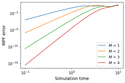
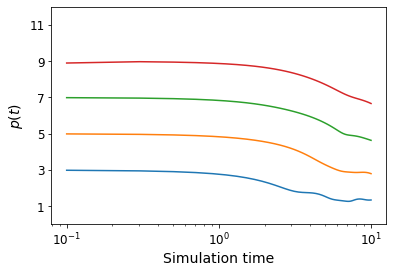
Figure 3: (left) Multiproduct errors plotted against simulation time, for several low-order MPFs, on a log-log plot. Notice the power law scaling for small values of $t$. The parameters used here are $B=1,\omega=4$, $\theta=\pi/6$. For larger $M$, one quickly runs into machine precision becoming the dominant error source. (right) The running power $p(t,t^{\prime})$ defined in equation (134), with $t^{\prime}=.3$. Note the plateau corresponds with the anticipated value of $2M+1$.

Next, we vary the MPF order $M$ for fixed simulation time $t$. Since $\Lambda=\omega$, our bounds predict an exponential decay in the error, but only provided $t<1/\omega$. Otherwise, the bounds grow exponentially and say nothing useful about performance. In Figure 4, we fix $t$ at several different times and plot the error dependence on the multiproduct order $M$. Past a certain threshold value for $M$ (which increases with $t$) an exponential decay in error is observed, possibly superexponential. It is promising that, even for $t=10$, the exponential decay is eventually achieved at $M\gtrsim 6$. This suggests our error bounds may be too conservative, and in particular MPFs could absolutely converge to $U$ as $M\rightarrow\infty$ in certain circumstances. This would be a notable improvement to product formulas alone, which tend to lead to errors that diverge as $M\rightarrow\infty$ if the time step $t$ remains fixed [2, 25, 4]. In contrast, Theorem 2 shows that if the time step is sufficiently small, then the MPF converges to the exact result. However, such convergence is not anticipated from the bounds for a large value such as $t=10$.

Indeed, there are good reasons to believe the absolute convergence property holds more generically than this example. No matter how large the order $M$, we are still using a low order formula (such as the midpoint formula $U_{2}$) as a base. Moreover, recall that the MPF is essentially a sum of product formulas with different numbers of time steps (for the same time interval). As the order $M$ increases, higher weight is given to terms in the multiproduct sum with finer meshes. Correspondingly, terms which have larger time steps, and therefore may not converge properly, become suppressed at large $M$. Such behavior is not reflected in our derived error bounds, so there is likely room for improvement.

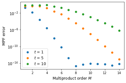
Figure 4: Multiproduct error shows an (super)exponential decrease in error for sufficiently large order $M$. The threshold for this regime is seen to increase as the simulation time increases. This behavior surpasses the expectation of our proven bounds, since there are no guarantees if the time step is too large. Note that, in practice, one should typically split a longer simulation time into smaller steps. The plateau for $t=1,M>8$ is a result of machine precision limitations. Parameter values: $B=1,\omega=4,\theta=\pi/6$.

Practitioners in quantum simulation will likely want to know how MPFs fare against the more-familiar and simpler Trotter techniques. To facilitate this, numerical studies across a broad range of physically interesting systems would be desirable. Such a comprehensive analysis must be left to future work; here we will be satisfied with comparing MPFs with Trotterization for our spin-1/2 example. Our Trotterization is just an MPF with $M=1$, corresponding to a midpoint-formula approximation. To facilitate a “fair-comparison” we will keep the number of midpoint-formula queries between the two methods the same. That is, we will enforce the requirement

$$r_{trot}=r_{mp}\max_{j}|k_{j}|$$ (135)

where $r_{trot}$ and $r_{mp}$ are the number of time steps for Trotter and MPF, respectively. Note that the number of midpoint queries per time step for Trotter and MPFs are 1 and $\max_{j}|k_{j}|$ respectively.

Figure 5 shows the results of these head-to-head comparisons for the several values of the magnetic field $B$ and rotation frequency $\omega$. The number of MPF steps $r_{mp}$ is fixed at 10, a reasonable value since it makes $\Lambda\Delta t\sim 1$ on each subinterval. As the MPF order increases, so does the number of Trotter steps $r_{trot}$ by the condition (135). These results show that, for $M$ not too large, MPFs outperform Trotterization, at a value of the error $\epsilon$ which is large enough to be of practical significance for scientific or industrial applications.

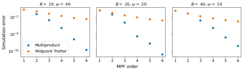
Figure 5: Simulation error (spectral norm) of MPFs and midpoint-formula Trotterization, for the spin-1/2 system, with number of midpoint-formula queries kept fixed between the two. Each plot corresponds to different values for the parameters $B$ and $\omega$, always with $\theta=\pi/6$. The number of MPF steps $r_{mp}$ is fixed at 10. The crossover point tends to occur for error $\epsilon>10^{-3}$, which is large enough for practical significance. Such error tolerances can be orders of magnitude larger than those required in many quantum simulation proposals. [8, 10]

Admittedly, the spin-1/2 system considered above is rather simplistic. However, we anticipate most of the inferences drawn above to hold even as we increase the dimensionality of the Hilbert space. For example, though the complexity of simulating $U_{2}$ generally increases as $\dim(H)$ grows, it does so both for MPFs and Trotterization. Nevertheless, benchmarking of MPFs on more complex systems would be a welcomed proof (or disproof) of concept.

8.2 Example 2: Spin chain in interaction picture

As a first step towards more complicated many-body quantum systems, we investigate the use of MPFs for a particular one-dimensional chain of spins with nearest-neighbor interactions. As before, we will take advantage of a change of reference frame, allowing us to compare the multiproduct simulations with an “exact” (machine precision) simulation in an equivalent, time-independent frame. In pursuit of a good case study, we seek a (time-independent) Hamiltonian $H=H_{0}+H_{1}$ which produces nontrivial time-dependence in the so-called “interaction picture.” We also ask that it satisfies a simple conservation law. A special instance of the 1D $XX$ model will suffice to meet these conditions. Consider a circular chain of $N$ qubits with nearest-neighbor hopping interactions, with Hamiltonian $H=H_{0}+H_{1}$ of the form

$$\begin{aligned} H_{0}&=\sum_{k=1}^{N}\frac{\omega_{k}}{2}Z_{k}\\ H_{1}&=\sum_{k=1}^{N}\frac{J_{k}}{2}\left(X_{k}X_{k+1}+Y_{k}Y_{k+1}\right).\end{aligned}$$ (136)

Here, $\omega_{k},J_{k}$ are real, site-dependent parameters, and any index increments are done modulo $N$. For any value of the parameters, the Hamiltonian conserves the total magnetization $\mu:=\sum_{k}Z_{k}$.

$$[\mu,H]=0$$ (137)

Conceptually will think of $H_{0}$ as a “base” Hamiltonian, with perturbation $H_{1}$ generating interactions, though we make no assumptions as to the smallness of $H_{1}$. We will switch to an interaction picture which is comoving with the simple dynamics of $H_{0}$. In this frame, the Hamiltonian $\tilde{H}(t)$ is given by

$$\begin{aligned} \tilde{H}(t)&=e^{iH_{0}t}H_{1}e^{-iH_{0}t}\\ &=\sum_{k=1}^{N}\frac{J_{k}}{2}\left(X_{k}(t)X_{k+1}(t)+Y_{k}(t)Y_{k+1}(t)\right)\end{aligned}$$ (138)

where

$$\begin{aligned} X_{k}(t)&:=e^{iH_{0}t}X_{k}e^{-iH_{0}t}=\cos(\omega_{k}t)X_{k}-\sin(\omega_{k}t)Y_{k}\\ Y_{k}(t)&:=e^{iH_{0}t}Y_{k}e^{-iH_{0}t}=\cos(\omega_{k}t)Y_{k}+\sin(\omega_{k}t)X_{k}\end{aligned}$$ (139)

correspond to rotating the pauli vectors about the $z$-axis with frequency $\omega_{k}$. We can express equation (138) in terms of the time-independent $X_{k}$ and $Y_{k}$ of the original frame,

$$\tilde{H}(t)=\sum_{k=1}^{N}\frac{J_{k}}{2}\big{\{}\cos(\Delta\omega_{k}t)(X_{k}X_{k+1}+Y_{k}Y_{k+1})+\sin(\Delta\omega_{k}t)(X_{k}Y_{k+1}-Y_{k}X_{k+1})\big{\}},$$ (140)

where $\Delta\omega_{k}=\omega_{k+1}-\omega_{k}$. We see that having different qubit frequencies $\omega_{k}$ on neighboring sites should give rise to a nontrivial time-dependence in $\tilde{H}$. Another indication is gleaned from the commutator of $H_{0}$ and $H_{1}$.

$$[H_{0},H_{1}]=-i\sum_{k}\frac{J_{k}}{2}(X_{k}Y_{k+1}-Y_{k}X_{k+1})(\Delta\omega_{k}).$$ (141)

The time dependence in $\tilde{H}$ will be nontrivial when the commutator does not vanish, as occurs when $\Delta\omega_{k}\neq 0$. A simple choice is to set

$$J_{k}=J,\quad\omega_{k}=(-1)^{k}\omega.$$ (142)

That is, the qubit frequency alternates sign at each site, and the coupling is translation invariant. For simplicity, we consider only even numbers of qubits to avoid frequency-matching at $k=N$. Plugging (142) into the expression for $\tilde{H}$ in (140),

$$\tilde{H}(t) =\frac{J}{2}\big{(}\cos(2\omega t)G_{1}+\sin(2\omega t)G_{2}\big{)}$$ (143)

where

$$\begin{aligned} G_{1}&=\sum_{k=1}^{N}X_{k}X_{k+1}+Y_{k}Y_{k+1}\\ G_{2}&=\sum_{k=1}^{N}(-1)^{k}(X_{k}Y_{k+1}-Y_{k}X_{k+1})\end{aligned}$$ (144)

As a final check, one can see that $G_{1}$ and $G_{2}$ do not commute with each other. Yet they both commute with $\mu$. Thus, $\tilde{H}(t)$ given in (143) is our model system to investigate.

Assuming $\tilde{H}$ commutes with an observable $\mu$, to what degree does the MPF $U_{\vec{k}}$ conserve $\mu$? Since $U_{\vec{k}}$ is an algebraic combination of exponentials of $\tilde{H}$, $U_{\vec{k}}$ also commutes with $\mu$. If $U_{\vec{k}}$ were truly unitary, then the operator $\mu$ would evolve in the Heisenberg picture as

$$\mu_{\vec{k}}(t)\equiv U_{\vec{k}}^{\dagger}(t)\mu U_{\vec{k}}(t)=\mu$$ (145)

as it would under the exact propagator $U$. However, $U_{\vec{k}}$ is not necessarily unitary.

$$U_{\vec{k}}^{\dagger}(t)U_{\vec{k}}(t)\neq\mathbb{1}$$ (146)

This implies that conservation laws are only approximately conserved.

$$\mu_{\vec{k}}(t)-\mu=\left(U_{\vec{k}}^{\dagger}(t)U_{\vec{k}}(t)-\mathbb{1}\right)\mu\neq 0.$$ (147)

Because $U_{\vec{k}}(t)-U(t)\in O(t^{2M+1})$, so is $\left(U_{\vec{k}}^{\dagger}(t)U_{\vec{k}}(t)-\mathbb{1}\right)$.

Figure 6 plots the deviations in the conserved $\mu$, $\norm{\mu-\mu_{\vec{k}}(t)}$, with respect to the simulation time. As the simulation time tends to zero, we see the expected power-law scaling, as evidence by the linear relationship on a log-log plot. For larger $M$, the slope and hence power $p$ increases, corresponding to improved performance. We can extract the power as the slope of the line, and this is plotted in the right frame. Notice there are sudden dips in the error at specific simulation times, which tend to occur before reaching the power law scaling regime. This could be due to cancellation between two terms in an error series of comparable magnitude. Similar phenomenon occurs in several other contexts, such as the error from adiabatic evolution [47]. Conclusive identification of these phenomenon will require further study.

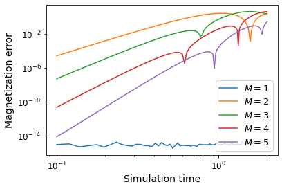
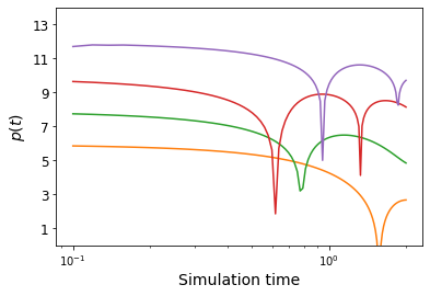
Figure 6: (left) Deviations from the conservation of magnetization $\mu$ under time-evolution by MPFs. Note that the order $M=1$ is simply a product formula evolution, which conserves $\mu$ exactly. For small simulation times, the expected power-law scaling is observed, with larger powers as $M$ increases. (right) The running power $p(t,t^{\prime})$ as defined in (134), with $t^{\prime}=.3$. Note the plateau at $2M+2$, which indicates slightly better convergence than naively expected ($p=2M+1$). This phenomenon generalizes to other systems and is formalized by Theorem 1. Parameter values: $N=4$, $J=1$, $\omega=4$

Naively, we would expect $p=2M+1$, but here we actually get slightly better: $p=2M+2$. In fact, this scaling can be justified. The following argument, a variant of which can be found in [31], shows that the integrator is nearly unitary.

Theorem 1.

The deviation of $U_{\vec{k}}$ from being unitary obeys

$$\|U_{\vec{k}}^{\dagger}(t)U_{\vec{k}}(t)-\mathbb{1}\|\in O(t^{2M+2})$$ (148)

Proof.

We suppress all function evaluations at $t$ when convenient. Let $E:=U_{\vec{k}}-U$, so that $U_{\vec{k}}=U+E$. Then, using the unitarity of $U$ and the fact that $E\in O(t^{2M+1})$,

$$U^{\dagger}_{\vec{k}}U_{\vec{k}}=\mathbb{1}+N+O(t^{4M+2})$$ (149)

where

$$N:=U^{\dagger}E+E^{\dagger}U.$$ (150)

Since $N\in O(t^{2M+1})$, all of its derivatives up to degree $2M$ vanish when evaluated at $t=0$. Hence, it suffices to show that

$$N^{(2M+1)}(0)=0.$$ (151)

We can expand this derivative in terms of $E$ and $U$ using the binomial theorem. When we evaluate at $t=0$, those terms with derivative less than degree $2M+1$ in $E$ vanish. We are left with

$$N^{(2M+1)}(0)=E^{\dagger(2M+1)}(0)U(0)+U^{\dagger}(0)E^{(2M+1)}(0).$$ (152)

We have $U(0)=U^{\dagger}(0)=\mathbb{1}$. Moreover, by the time-symmetric property of $U$ and $U_{\vec{k}}$, $E(t)$ is also symmetric. Therefore

$$E^{\dagger(2M+1)}(0)=E^{(2M+1)}(-t)\Big{\rvert}_{t=0}=-E^{(2M+1)}(0).$$ (153)

Hence, the two terms in (152) cancel, yielding $N^{(2M+1)}(0)=0$. This completes the proof. ∎

In summary, though MPFs do not inherently preserve commutations laws, the error is due to nonunitarity in $U_{\vec{k}}$. This can be bounded and reduced in a systematic way, either by decreasing the time step or increasing the MPF order.

9 Conclusion

The main contribution of this paper is a new way of thinking about time-dependent dynamics that allows us to replace time-ordered operator exponentials with ordinary operator exponentials acting on a higher-dimensional finite space. The resultant operators are bounded, which allows us to rigorously apply the technique (in contrast to previous attempts [29] to employ related strategies). We apply this trick to adapt the MPF formalism to the time-dependent case, and in turn provide a method that not only has commutator scaling, but also outperforms time-dependent Trotter-Suzuki methods. Further, we show that as the dimensionality of the clock space grows, the entanglement between the clock and system vanishes. This means that in the continuum limit, the gadgetry introduced to approximate the time-ordered operator exponential becomes irrelevant, allowing us to use the resulting formulae while dispensing with the fictitious clock register used to implement the time-ordering.

The clock space framework can also be used directly in quantum simulation methods to extend the capabilities of certain quantum algorithms. Specifically, it can be used to extend qubitization to time-dependent systems, the intuition behind which has resisted previous attempts to do so. We find here that for problems that have small second derivatives for the Hamiltonian, qubitization can be used to simulate the controlled Hamiltonian that we use in the clock space evolution approximating the exact propagator. While in many circumstances it will be more convenient to use a truncated Dyson series simulation method in preference to this approach, our work shows how the use of discrete clock spaces used to construct new quantum simulation algorithms that would otherwise be challenging.

To complement our theoretical results, we present several numerical examples which demonstrate that MPFs can perform better than our bounds suggest, and also better than low-order product formula simulations. There is a possibility that MPFs converge to the propagator in the limit of large order $M$ regardless of the time step size, assuming sufficient smoothness in $H$. The corresponding statement is not true for Trotter-Suzuki: smaller and smaller time intervals must be taken to ensure convergence as one reaches higher order formulas. Proving (or disproving) absolute convergence would be a valuable avenue for future research. Though the examples presented here have physical relevance and provide a strong proof of concept, numerical tests of MPFs on a larger class of more challenging physical systems would be desirable.

This work opens up a number of interesting possibilities. The first is that while the techniques considered here are adequate for translating algorithms for time-independent simulation to the time-dependent case, the methods have not been optimized to reduce the resources needed. The development of higher-order methods for simulations could potentially render these approaches more profitable by reducing the norm of the time-displacement operator needed in the simulation, thereby making the simulation more efficient. Another open question raised by this work is whether these techniques could be used to translate commutator bounds from a recent work[4] over to the time-dependent case. This would be a significant step towards the development of a complete understanding of the error in Trotter-Suzuki formulas, since for the first time we would have a bound on the error of ordered operator exponentials that yields the anticipated commutator scaling.

Acknowledgments

We thank Jeffrey Schenker and Dominic Berry for helpful discussions. This work was supported in part by the U.S. Department of Energy (DOE), Office of Science, Office of Nuclear Physics, Inqubator for Quantum Simulation (IQuS) under Award Number DOE (NP) Award DE-SC0020970, as well as awards DE-SC0021152 and DE-SC0013365, and by the National Science Foundation Graduate Research Fellowship under Grant No. DGE-1848739. NW’s work on this project is supported by ”Embedding Quantum Computing into Many-body Frameworks for Strongly Correlated Molecular and Materials Systems” project, which is funded by the DOE Office of Science, Office of Basic Energy Sciences, the Division of Chemical Sciences, Geosciences, and Biosciences.

Appendix A Proof of bounds on multiproduct Taylor remainder

Here we provide the proof of Lemma 3, which bounds the Taylor remainder $R_{2M}$ of the MPF $U_{\vec{k}}$. For clarity, the proof outline is as follows.

1. In Lemma 1, we bound the derivatives of the constituent midpoint formulas $U_{2}$ in the MPF.

2. Using this result, in Lemma 2 we bound the derivatives of $U_{\vec{k}}$ itself.

3. From here, it is quite straightforward to get a bound on $R_{n}$ for any $n\geq 0$. This is quickly proved in Lemma 3

4. The proof of Lemma 3 follows from a simplification of this bound to a form more suitable for the complexity analysis done in the paper.

Without further ado, we will begin the program outlined above, starting with our $U_{2}$ derivatives.

Lemma 1.

Let $U_{2}:(\mathbb{R},\mathbb{R})\rightarrow\mathbb{C}^{N\times N}$ be the midpoint formula as given by equation (13). Let $k\in\mathbb{Z}_{+}$ and $q\in\mathbb{Z}_{+}$ such that $q\leq k$. Let $t_{0}\in\mathbb{R}$, and let $\Delta t\in\mathbb{R}_{+}$ be chosen sufficiently small such that

$$\Lambda_{I}:=\max_{\tau\in I}\Lambda(\tau)<1/\Delta t,$$ (154)

where $I=[t_{0},t_{0}+\Delta t]$ is the full simulation interval. Then the following inequality holds

$$\norm{\partial_{\Delta t}^{n}U_{2}(t_{0}+q\Delta t/k,t_{0}+(q-1)\Delta t/k)}\leq\left(\Lambda_{q}\frac{q-1/2}{k}\right)^{n}Y_{n}\left(\vec{x}^{(n)}_{q,k}\right).$$ (155)

In the above expression, $\Lambda_{q}$ is the maximum value of $\Lambda(\tau)$ over the $q^{\rm th}$ subinterval in a evenly spaced mesh of $k$ subintervals in $[t_{0},t_{0}+\Delta t]$. $Y_{n}$ is the complete exponential Bell polynomial (see Appendix B) and $\vec{x}^{(n)}_{q,k}=(x_{1},\dots,x_{n})\in\mathbb{Q}_{+}^{n}$ has coefficients defined by

$$x_{j}=\frac{j}{q-1/2}+\frac{1}{k}$$ (156)

Proof.

To simplify matters, let’s for the moment consider the midpoint formula $U_{2}(\Delta t)$ only as a function of $\Delta t$. Define

$$A(\Delta t):=-iH\big{(}t_{0}+(q-1/2)\Delta t/k\big{)}\Delta t/k,$$ (157)

so that

$$U_{2}(\Delta t)=\exp(A(\Delta t)).$$ (158)

To compute the left-hand side of inequality (155), we wish to take high-order derivatives of $\exp(A(\Delta t))$. Unfortunately, this is complicated by $A(\Delta t)$ being an operator-valued function. To illustrate this, one expression for the derivative of the exponential map given by

$$\partial_{\Delta t}\exp(A(\Delta t))=\int_{0}^{1}e^{A(\Delta t)(1-s)}A^{\prime}(\Delta t)e^{A(\Delta t)s}ds.$$ (159)

When comparing to the scalar valued exponential, the extra integral can be seen to arise from $A^{\prime}$ not necessarily commuting with $A$, forcing us to “insert” $A^{\prime}$ at different places and “sum” over all placements. This result can be bounded using the submultiplicative property of the spectral norm, but in order to do so we need a method for bounding the higher-order derivatives of $A$.

Since $[A,A^{\prime}]$ is not necessarily zero, we cannot immediately apply the Faà di Bruno formula (209) for the derivative. Despite this problem, it is easy to see from the triangle inequality that for anti-Hermitian $A$, $\|\partial_{\Delta t}\exp(A(\Delta t))\|\leq\|A^{\prime}(\Delta t)\|$. Thus we will seek a version of Faà di Bruno that provides an upper bound on the norm of the derivative of $e^{A(\Delta t)}$.

From the Trotter product theorem, we have

$$\partial_{\Delta t}^{n}\exp(A(\Delta t))=\partial_{\Delta t}^{n}\lim_{r\rightarrow\infty}(\exp(A(\Delta t)/r))^{r}.$$ (160)

Using the fact that the series converges uniformly, we may interchange the order of differentiation and the limit. This leads to

$$\|\partial_{\Delta t}^{n}\exp(A(\Delta t))\|\leq\lim_{r\rightarrow\infty}\sum_{S}\binom{n}{s_{1},\ldots,s_{r}}\prod_{q=1}^{r}\left\|\partial_{\Delta t}^{s_{q}}\exp(A(\Delta t)/r)\right\|.$$ (161)

Here the sum over $S$ is constrained such that $s_{j}\geq 0$ and $s_{1}+\cdots+s_{r}=n$. Then using Taylor’s theorem we have

$$\left\|\partial_{\Delta t}^{s_{q}}\exp(A(\Delta t)/r)\right\|\leq\frac{\|A^{(s_{q})}(\Delta t)\|}{r}+O(1/r^{2}).$$ (162)

where the $O(1/r^{2})$ terms will vanish as $r\rightarrow\infty$. Hence,

$$\|\partial_{\Delta t}^{n}\exp(A(\Delta t))\|\leq\lim_{r\rightarrow\infty}\sum_{S}\binom{n}{s_{1},\ldots,s_{r}}\prod_{q=1}^{r}\left(\frac{\|A^{(s_{q})}(\Delta t)\|(1-\delta_{s_{q},0})}{r}+\delta_{s_{q},0}\right).$$ (163)

Now let us define a scalar function $a(t)$ such that, for any $n\geq 0$,

$$a^{(n)}(\Delta t)=\|A^{(n)}(\Delta t)\|\delta_{n,0}.$$ (164)

for fixed $\Delta t$. Such a function can be seen to exist by considering the Taylor polynomial. We may apply the standard Faà di Bruno formula (209) to $a$, so that

$$\partial_{t}^{n}e^{a(\Delta t)}=e^{a(\Delta t)}Y_{n}(\|A^{(1)}(\Delta t)\|,\dots,\|A^{(n)}(\Delta t)\|)=Y_{n}(\|A^{(1)}(\Delta t)\|,\dots,\|A^{(n)}(\Delta t)\|).$$ (165)

On the other hand, applying similar logic to that employed above, we can split the scalar function $a(t)$ into $r$ steps and compute the $n$th derivative.

$$\partial_{t}^{n}e^{a(\Delta t)}=\lim_{r\rightarrow\infty}\sum_{S}\binom{n}{s_{1},\ldots,s_{r}}\prod_{q=1}^{r}\left(\frac{\|A^{(s_{q})}(\Delta t)\|(1-\delta_{s_{q},0})}{r}+\delta_{s_{q},0}\right)$$ (166)

By equating expressions (163) and (166) and applying (165), we reach our desired bound via Faà di Bruno.

$$\|\partial_{\Delta t}^{n}\exp(A(\Delta t))\|\leq Y_{n}(\|A^{(1)}(\Delta t)\|,\dots,\|A^{(n)}(\Delta t)\|)$$ (167)

We evaluate the derivatives of $A(\Delta t)$, and express them in terms of the derivatives of the Hamiltonian, $H^{(j)}$ (for simplicity, we leave off the evaluation point. The derivative is with respect to the Hamiltonian’s single argument). The result is

$$\partial_{\Delta t}^{j}A(\Delta t)=\frac{-i}{k}\left[\left(\frac{q-1/2}{k}\right)^{j}\Delta tH^{(j)}+j\left(\frac{q-1/2}{k}\right)^{j-1}H^{(j-1)}\right]$$ (168)

Employing the $\Lambda(\tau)$ bound in Definition 1, we have that

$$\begin{aligned} \norm{\partial_{\Delta t}^{j}A(\Delta t)}&\leq\frac{1}{k}\left[\left(\frac{q-1/2}{k}\right)^{j}\Lambda_{q}^{j+1}\Delta t+j\left(\frac{q-1/2}{k}\right)^{j-1}\Lambda_{q}^{j}\right]\\ &=\left(\frac{q-1/2}{k}\right)^{j}\Lambda_{q}^{j}\left[\frac{j}{q-1/2}+\frac{1}{k}\Lambda_{q}\Delta t\right].\end{aligned}$$ (169)

Here,

$$\Lambda_{q}:=\max_{\Delta t\in I_{q}}\Lambda(\Delta t)$$ (170)

where $I_{q}=[t_{0}+(q-1)\Delta t/k,t_{0}+q\Delta t/k]$ is the $q$th interval in the mesh from $t_{0}$ + $t_{0}+\Delta t$ with $k$ even spaces. Since $\Lambda_{q}\leq\Lambda_{I}$, from the assumptions of the lemma, $\Lambda_{q}\Delta t<1$. Hence,

$$\begin{aligned} \norm{\partial_{\Delta t}^{j}A(\Delta t)}&\leq\tilde{\Lambda}_{q}^{j}\left[\frac{j}{q-1/2}+\frac{1}{k}\right]\\ \end{aligned}$$ (171)

where $\tilde{\Lambda}_{q}\equiv\Lambda_{q}(q-1/2)/k$.

Plugging this into the formula into (167) and using the definition of $Y_{n}$ given by (210), our bound becomes

$$\norm{\partial_{\Delta t}^{n}U_{2}(\Delta t)}\leq\sum_{C}\frac{n!}{c_{1}!\dots c_{n}!}\prod_{j=1}^{n}\left(\frac{(\frac{j}{q-1/2}+\frac{1}{k})\tilde{\Lambda}_{q}^{j}}{j!}\right)^{c_{j}}.$$ (172)

Using the sum property of the coefficients $c_{j}$, we can move the $\tilde{\Lambda}_{q}^{j}$ out of the sum.

$$\norm{\partial_{\Delta t}^{n}U_{2}(\Delta t)} \leq\left(\Lambda_{q}\frac{q-1/2}{k}\right)^{n}\sum_{C}\frac{n!}{c_{1}!\dots c_{n}!}\prod_{j=1}^{n}\left(\frac{\frac{j}{q-1/2}+\frac{1}{k}}{j!}\right)^{c_{j}}$$ (173)

$$=\left(\Lambda_{q}\frac{q-1/2}{k}\right)^{n}Y_{n}\left(\vec{x}_{q,k}^{(n)}\right).$$ (174)

In the last line, we reapplied the definition of $Y_{n}$ and of the vectors $\vec{x}_{q,k}^{(n)}$. This completes our bound for the $U_{2}$ formula for the $q$th segment of mesh defined by $k_{j}$. ∎

Lemma 2.

In the notation of Lemma 1, the $n^{\rm th}$ derivative of the $M$-term multiproduct formula $U_{\vec{k}}$ with respect to $\Delta t$ has spectral norm which is bounded as

$$\norm{U_{\vec{k}}^{(n)}(t_{0}+\Delta t,t_{0})}\leq n!\Lambda_{I}^{n}\sum_{j=1}^{M}\absolutevalue{a_{j}}\beta_{k_{j}}^{(n)}$$ (175)

where

$$\beta_{k_{j}}^{(n)}:=\sum_{S}\prod_{q=1}^{k_{j}}\frac{1}{s_{q}!}\left(\frac{q-1/2}{k_{j}}\right)^{s_{q}}Y_{s_{q}}\left(\vec{x}^{(s_{q})}_{q,k_{j}}\right)$$ (176)

and the sum $\sum\limits_{S}$ is taken over all nonnegative $s_{1},s_{2},\dots,s_{n}$ such that $\sum_{j}s_{j}=n$.

Proof.

For sake of shorter expressions, define $\Delta t_{j}=\Delta t/k_{j}$. From Definition 5,

$$\begin{aligned} \partial_{\Delta t}^{n}U_{\vec{k}}(t_{0}+\Delta t,t_{0})&=\sum_{j=1}^{M}a_{j}\partial_{\Delta t}^{n}\prod_{q=1}^{k_{j}}U_{2}(t_{0}+q\Delta t_{j},t_{0}+(q-1)\Delta t_{j})\end{aligned}$$ (177)

Now we use the product rule and apply Lemma 1 to obtain

$$\norm{\partial_{\Delta t}^{n}U_{\vec{k}}(t_{0}+\Delta t,t_{0})}\leq\sum_{j=1}^{M}\absolutevalue{a_{j}}\left(\sum_{S}\binom{n}{s_{1},\dots,s_{k_{j}}}\prod_{q=1}^{k_{j}}\left(\frac{q-1/2}{k_{j}}\Lambda_{q,k_{j}}\right)^{s_{q}}Y_{s_{q}}\left(\vec{x}_{q,k_{j}}^{(s_{q})}\right)\right).$$ (178)

where $\Lambda_{q,k_{j}}$ is the maximum of $\Lambda(\tau)$ on $[t_{0}+(q-1)\Delta t/k_{j},t_{0}+q\Delta t/k_{j}]$. Of course, this is upper bounded by the max of $\Lambda$ over the whole interval $I$.

$$\Lambda_{q,k_{j}}\leq\Lambda_{I}$$ (179)

Replacing every instance of $\Lambda_{q,k_{j}}$ with $\Lambda_{I}$ as an upper bound, it can factored all the way out, using the sum properties of the $s_{q}$.

$$\norm{\partial_{\Delta t}^{n}U_{\vec{k}}(t_{0}+\Delta t,t_{0})}\leq\Lambda_{I}^{n}\sum_{j=1}^{M}\absolutevalue{a_{j}}\sum_{S}\binom{n}{s_{1},\dots,s_{k_{j}}}\prod_{q=1}^{k_{j}}\left(\frac{q-1/2}{k_{j}}\right)^{s_{q}}Y_{s_{q}}\left(\vec{x}_{q,k_{j}}^{(s_{q})}\right).$$ (180)

Finally, we factor out a factor of $n!$, for later convenience. Writing out the multinomial, we identify the remaining sum as our $\beta_{k_{j}}^{(n)}$ coefficient. This completes the lemma. ∎

Lemma 3.

In the assumptions and notation of Lemma 1, let $R_{n}$ be the Taylor remainder operator over $I$ as in equation (58). The following bound on the spectral norm of $R_{n}$ holds.

$$\norm{R_{n}(t_{0}+\Delta t,t_{0})}\leq\left(\Lambda_{I}\Delta t\right)^{n+1}\sum_{j=1}^{M}\beta_{k_{j}}^{(n+1)}\absolutevalue{a_{j}}$$ (181)

Proof.

By the triangle inequality for integrals,

$$\begin{aligned} \norm{R_{n}(t_{0}+\Delta t,t_{0})}&=\norm{\frac{1}{n!}\int_{0}^{\Delta t}(\Delta t-\tau)^{n}U_{\vec{k}}^{(n+1)}(t_{0}+\tau,t_{0})d\tau}\\ &\leq\frac{1}{n!}\int_{0}^{\Delta t}(\Delta t-\tau)^{n}\norm{U_{\vec{k}}^{(n+1)}(t_{0}+\tau,t_{0})}d\tau\end{aligned}$$ (182)

We can upper bound the norm inside the integral using the results from the previous lemma. But these bounds will depend on $\tau$. However, careful examination shows that the only dependence is implicitly in $\Lambda_{I}$, where it defines the interval of maximization. Thus, $\Lambda_{I}$ is monotonically increasing with $\tau$, and so we may yet again upper bound by choosing the integration endpoint $\tau=\Delta t$. Thus,

$$\begin{aligned} \norm{R_{n}(t_{0}+\Delta t,t_{0})}&\leq\frac{(n+1)!}{n!}\Lambda_{I}^{n+1}\sum_{j=1}^{M}\beta_{k_{j}}^{(n+1)}\absolutevalue{a_{j}}\int_{0}^{\Delta t}(\Delta t-\tau)^{n}d\tau\\ &=(\Lambda_{I}\Delta t)^{n+1}\sum_{j=1}^{M}\beta_{k_{j}}^{(n+1)}\absolutevalue{a_{j}}\end{aligned}$$ (183)

This proves our result. ∎

Finally, we are ready to obtain the sought-after proof of the bounds presented in Section 4 on the Taylor remainder $R_{2M}$.

Proof of Lemma 3.

Consider the $\beta_{k}^{(n)}$ coefficients in equation (176). As a starting simplification, we have $(q-1/2)/k<1$ in all instances. This gives,

$$\beta_{k}^{(n)}<\sum_{S}\prod_{q=1}^{k}\frac{1}{s_{q}!}Y_{s_{q}}\left(\frac{[s_{q}]}{q-1/2}+\frac{1}{k}\right)$$ (184)

Furthermore, we have

$$Y_{s_{q}}\left(\frac{[s_{q}]}{q-1/2}+\frac{1}{k}\right)<B_{s_{q}}\left(\frac{s_{q}}{q-1/2}+\frac{1}{k}\right),$$ (185)

where $B_{n}(x)$ is the $n$th Bell polynomial (or Touchard polynomial), a single variable function defined evaluating $Y_{n}$ the same in every variable (see Appendix B for details). In the special case where $s_{q}=0$, $B_{s_{q}}=1$ and does not affect the product. Therefore we can leave it out of the subsequent analysis and assume $s_{q}>0$. Using the results from [49], for any such $s_{q}$,

$$B_{s_{q}}\left(\frac{s_{q}}{q-1/2}+\frac{1}{k}\right)\leq\left(\frac{s_{q}}{\log(1+\frac{s_{q}}{\frac{s_{q}}{q-1/2}+1/k})}\right)^{s_{q}}\leq(4s_{q})^{s_{q}}$$ (186)

Similarly, Stirling’s formula states that

$$\frac{1}{s_{q}!}<\frac{1}{\sqrt{2\pi s_{q}}}\left(\frac{e}{s_{q}}\right)^{s_{q}}.$$ (187)

Employing the two bounds above,

$$\beta_{k}^{(n)}<\sum_{S}\prod_{q=1}^{k}\frac{1}{\sqrt{2\pi s_{q}}}\left(4e\right)^{s_{q}}=\frac{(4e)^{n}}{(2\pi)^{k/2}}\sum_{S}\prod_{q=1}^{k}\frac{1}{\sqrt{s_{q}}}\leq\frac{(4e)^{n}}{(2\pi)^{k/2}}\sum_{S}(1)$$ (188)

where we used the summation property of the $s_{q}$ (true even when leaving out $s_{q}=0$). This sum counts the number of ways the $\{s_{q}\}_{q=1}^{k}$ can add to $n$. The result is a particular binomial, also seen in counting bosonic states.

$$\beta_{k}^{(n)}<\frac{(4e)^{n}}{(2\pi)^{k/2}}\binom{n+k-1}{k-1}.$$ (189)

Applying this simplified bound on $\beta$ to Lemma 3 gives a much-simplified remainder bound.

$$\norm{R_{n}(t_{0}+\Delta t,t_{0})}<\left(4e\max_{\tau\in[t_{0},t_{0}+\Delta t]}\Lambda(\tau)\Delta t\right)^{n+1}\sum_{j=1}^{M}\frac{\absolutevalue{a_{j}}}{(2\pi)^{k_{j}/2}}\binom{n+k_{j}}{k_{j}-1}$$ (190)

For a fixed $n$, the binomial coefficient above grows with monotonically $k_{j}$. This can be seen by writing

$$\binom{n+k_{j}}{k_{j}-1}=\frac{(n+k_{j})!}{(n+1)!(k_{j}-1)!}=\frac{(n+k_{j})(n+k_{j}-1)\dots(k_{j})}{(n+1)!}$$ (191)

On the right side, the numerator increases with $k_{j}$ while the denominator remains fixed. However, the factor $(2\pi)^{-k_{j}/2}$ largely compensates this growth. In order to see this, we first use Stirling’s formula to bound the binomial.

$$\begin{split}\binom{n+k}{k-1}&\leq\frac{1}{\sqrt{2\pi}}\sqrt{\frac{n+k}{(k-1)(n+1)}}\frac{(n+k)^{n+k}}{(n+1)^{n+1}(k-1)^{k-1}}\exp\left(\frac{1}{12(n+k)}-\frac{1}{12(n+1)+1}-\frac{1}{12(k-1)+1}\right)\\ &<\sqrt{\frac{1}{2\pi}}\sqrt{\frac{n+k}{(k-1)(n+1)}}\left(\frac{n+k}{n+1}\right)^{n+1}\left(\frac{n+k}{k-1}\right)^{k-1}\exp\left(\frac{1}{12(n+k)}-\frac{1}{12(n+1)+1}\right)\end{split}$$ (192)

The second line above uses the fact that $n>1$ and $k\geq 1$. Reintroducing the $(2\pi)^{-k/2}$ factor and noticing that the sum of the first two factors in the exponent is less than $1/600$, and $\exp(1/600)<1.002$, we have

$$\frac{1}{(2\pi)^{k/2}}\binom{n+k_{j}}{k_{j}-1}\leq\frac{1.002}{2\pi}\sqrt{\frac{n+k}{(k-1)(n+1)}}\left(\frac{n+k}{n+1}\right)^{n+1}\left(\frac{n+k}{\sqrt{2\pi}(k-1)}\right)^{k-1}\;.$$ (193)

In our application, we are interested in MPFs of order $2M$, hence we set $n=2M$. From [27] we then have that

$$k_{j}=\left\lceil\frac{\sqrt{8}M}{\pi}\absolutevalue{\sin\left(\frac{\pi(2j-1)}{8M}\right)}^{-1}\right\rceil.$$ (194)

We can now bound the coefficients using $\sin(x)\leq x$ and $\sin(x)\geq 4x/5$ for $x\in[0,1]$, which is satisfied in this case. This gives the lower bound

$$k_{j}\geq\left\lceil\frac{8^{3/2}M^{2}}{\pi^{2}(2j-1)}\right\rceil\geq\left\lceil\frac{8^{3/2}M^{2}}{\pi^{2}(2M-1)}\right\rceil>\frac{\sqrt{128}M}{\pi^{2}}>M=\frac{n}{2}\;$$ (195)

together with

$$k_{j}\leq\left\lceil\frac{5\times 8\sqrt{8}M^{2}}{4(2j-1)\pi^{2}}\right\rceil\leq\left\lceil\frac{5\times 8\sqrt{8}M^{2}}{4\pi^{2}}\right\rceil<3M^{2}\;.$$ (196)

Using the lowerbound, together with $n\geq 4$ (since $M>1$), we can get

$$\sqrt{\frac{n+k}{(k-1)(n+1)}}=\sqrt{\frac{1}{k-1}+\frac{1}{n+1}}\leq\sqrt{\frac{2}{n-2}+\frac{1}{n+1}}<\sqrt{\frac{6}{5}}\;.$$ (197)

Now we distinguish two cases. First let us assume that

$$n+k\geq\sqrt{2\pi}(k-1).$$ (198)

This implies that

$$n+k\leq(n+1)\left(1+\frac{1}{\sqrt{2\pi}-1}\right)$$ (199)

which combined with the lower bound on $k_{j}$ in (195) yields

$$\begin{split}\left(\frac{n+k}{n+1}\right)^{n+1}\left(\frac{n+k}{\sqrt{2\pi}(k-1)}\right)^{k-1}&\leq\left(\frac{\sqrt{2\pi}}{\sqrt{2\pi}-1}\right)^{n+1}\left(\frac{n+k}{\sqrt{2\pi}(k-1)}\right)^{\frac{n+1}{\sqrt{2\pi}-1}}\\ &\leq\left(\frac{\sqrt{2\pi}}{\sqrt{2\pi}-1}\right)^{n+1}\left(\frac{n+1}{(\sqrt{2\pi}-1)(k-1)}\right)^{\frac{n+1}{\sqrt{2\pi}-1}}\\ &\leq\left(\frac{\sqrt{2\pi}}{\sqrt{2\pi}-1}\right)^{n+1}\left(\frac{n+1}{(\sqrt{2\pi}-1)(n/2-1)}\right)^{\frac{n+1}{\sqrt{2\pi}-1}}\\ &\leq\left(\frac{\sqrt{2\pi}}{\sqrt{2\pi}-1}\right)^{n+1}\left(\frac{5}{\sqrt{2\pi}-1}\right)^{\frac{n+1}{\sqrt{2\pi}-1}}\\ &\leq 3.7^{n+1}\end{split}$$ (200)

where in the third line we used the lower bound $k>n/2$ and in the fourth the lower bound $n\geq 4$. Now let us consider the second case wherein

$$n+k<\sqrt{2\pi}(k-1)\Rightarrow(k-1)>(n+1)/(\sqrt{2\pi}-1)$$ (201)

Defining $(k-1)=\eta(n+1)$ with $\eta\geq 1/(\sqrt{2\pi}-1)$ so that

$$\begin{split}\left(\frac{n+k}{n+1}\right)^{n+1}\left(\frac{n+k}{\sqrt{2\pi}(k-1)}\right)^{k-1}&=\left(\left(1+\eta\right)\left(\frac{1+\eta}{\sqrt{2\pi}\eta}\right)^{\eta}\right)^{n+1}\\ &\leq\left(\frac{\sqrt{2\pi}}{\sqrt{2\pi}-1}\right)^{n+1}<3.7^{n+1}\end{split}$$ (202)

Then combining these two cases leads us to the following uniform upper bound

$$\frac{1}{(2\pi)^{k/2}}\binom{n+k_{j}}{k_{j}-1}<\frac{1.002}{2\pi}\sqrt{\frac{6}{5}}3.7^{n+1}<0.16\times 3.7^{n+1}\;.$$ (203)

Using this we can further upper bound the remainder as

$$\begin{split}\norm{R_{2M}(t_{0}+\Delta t,t_{0})}&<0.16\left(4e\times 3.7\max_{\tau\in[t_{0},t_{0}+\Delta t]}\Lambda(\tau)\Delta t\right)^{2M+1}\norm{a}_{1}\\ &<0.16\left(41\max_{\tau\in[t_{0},t_{0}+\Delta t]}\Lambda(\tau)\Delta t\right)^{2M+1}\norm{a}_{1}\end{split}$$ (204)

This last inequality, finally, has brought us to the sought after result of Lemma 3. ∎

Appendix B Mathematical tools and notation

The purpose of this section is as reference for some of the mathematical concepts and notation used throughout the paper. Subsection B.1 discusses several combinatorial definitions and results invoked in the paper, while Subsection B.2 discusses the vector, function, and operator norms used.

B.1 Combinatorics

Much of the technical work in this paper stems from computing high-order derivatives of products and composite functions, which essentially becomes an exercise in combinatorics. The purpose of this section is to introduce some of the combinatorics tools used in this analysis.

The multinomial coefficient is a generalization of the more-familiar binomial coefficient, and it arises in several combinatorial situations. For our purposes, it is defined by

$$\binom{n}{s_{1},...,s_{k}}:=\frac{n!}{s_{1}!s_{2}!...s_{k}!}$$ (205)

where $n\in\mathbb{Z}_{+}$ and the $(s_{q})_{q=1}^{k}$ are nonnegative integers which sum to $n$. It is always a positive integer, corresponding to the number of distinct ways of placing $n$ distinguishable items into $k$ boxes, where each box has a fixed number $s_{j}$ of items. In this work, we will find occasion to make use of the multinomial when high-order derivatives of a product.

$$\left(\frac{d}{dt}\right)^{n}f_{1}(t)f_{2}(t)\dots f_{k}(t)$$ (206)

Here, $(f_{q})_{q=1}^{k}$ are $n$-differentiable functions on an interval $I\subseteq\mathbb{R}$. Employing the product rule, one is left to count all the possible combinations of derivatives of each $f_{q}$. It turns out that the multinomial is suited for performing this counting.

$$\left(\frac{d}{dt}\right)^{n}\prod_{q=1}^{k}f_{q}(t)=\sum_{S}\binom{n}{s_{1},\dots,s_{k}}\prod_{q=1}^{k}\left(\frac{d}{dt}\right)^{s_{q}}f_{q}(t)$$ (207)

The sum is taken over the set $S$ of sequences of nonnegative integers $(s_{q})_{q=1}^{k}$ summing to $n$. As an aside, a similar multinomial sum to the above arises when taking $n$ powers of a sum of $k$ distinct variables. The same counting arguments are invoked.

On other occasions in the text below, we will be led to evaluate high-order derivatives of the exponential of a function $a(t)$.

$$\left(\frac{d}{dt}\right)^{n}e^{a(t)}$$ (208)

This problem is also of a combinatorial nature. The solution we will rely on is Faà di Bruno’s formula. In our specific context, this formula asserts that

$$\left(\frac{d}{dt}\right)^{n}e^{a(t)}=e^{a(t)}Y_{n}(a^{\prime}(t),a^{\prime\prime}(t),\dots,a^{(n)}(t))$$ (209)

where $Y_{n}$ is the complete exponential Bell polynomial. [50] An explicit formula is given by

$$Y_{n}(x_{1},x_{2},\dots,x_{n})=\sum_{C}\frac{n!}{c_{1}!c_{2}!\dots c_{n}!}\prod_{j=1}^{n}\left(\frac{x_{j}}{j!}\right)^{c_{j}}$$ (210)

where the sum is taken over the set $C$ of all sequences $(c_{j})_{j=1}^{n}$ such that $c_{j}\geq 0$ and

$$c_{1}+2c_{2}+\dots+nc_{n}=n.$$ (211)

Essentially, each coefficient in $Y_{n}$ counts the ways one can partition a set of fixed size $n$ into subsets of given sizes and number. When one simply wants to count the total number of possible partitions, one is led to the Bell numbers $b_{n}$. These are related to the $Y_{n}$ by evaluating all arguments to one.

$$b_{n}=Y_{n}(1,1,...1)$$ (212)

More generally, for any $x\in\mathbb{R}$,

$$Y_{n}(x,x^{2},\dots,x^{n})=x^{n}b_{n},$$ (213)

which can be seen directly from (210) along with the sum rule (211). The Bell numbers $b_{n}$ grow combinatorially, like a factorial. In fact, the following upper bound is invoked in the paper [37].

$$b_{n}<\left(\frac{.792n}{\log(n+1)}\right)^{n},\quad\forall n\in\mathbb{Z}_{+}$$ (214)

There is a natural way to form a single variable polynomial from $Y_{n}$ by evaluating all arguments to the same value $x$. This is sometimes called simply the Bell polynomial or Touchard polynomial $B_{n}(x)$.

$$B_{n}(x)=Y_{n}(x,x,\dots,x)$$ (215)

Of course, $b_{n}=B_{n}(1)$. The $n$th Bell polynomial $B_{n}(x)$ is also the value of the $n$th moment of the Poisson distribution with mean $x$. From [49] we have the following upper bound on $B_{n}$.

$$B_{n}(x)\leq\left(\frac{n}{\log(1+\frac{n}{x})}\right)^{n}$$ (216)

Notice that this bound for $x=1$ is very close to that for the Bell numbers in (214). From their definitions, and intuitively from their combinatorial natures, $Y_{n}$, $B_{n}$ and $b_{n}$ all grow monotonically, both in their functional arguments and their index $n$.

Compared to these special functions, the reader is likely more familiar with the simple factorial $n$! and it’s corresponding asymptotic expression given by Stirling’s approximation. In the paper, we always make use of a version of the approximation which gives strict bounds for $n>0$.

$$\sqrt{2\pi n}\left(\frac{n}{e}\right)^{n}<n!<\sqrt{2\pi n}\left(\frac{n}{e}\right)^{n}e^{1/(12n)}$$ (217)

These bounds are extremely good, even for small $n$.

B.2 Norms

There are a couple different types of norms employed throughout the paper, on a variety of mathematical objects. Here we define and discuss each of them.

The Schatten $p$-norm, is defined for any $v\in\mathbb{C}^{n}$, with any $n\in\mathbb{Z}_{+}$. It is defined as

$$\norm{v}_{p}:=\left(\sum_{j=1}^{n}\absolutevalue{v_{j}}^{p}\right)^{1/p}.$$ (218)

In the paper, we will make use of the 1-norm several contexts, such as the coefficients $a$ of the multiproduct formula.

$$\norm{v}_{1}:=\sum_{j}\absolutevalue{v_{j}}$$ (219)

In the main paper we claim our Hamiltonian simulation algorithm exhibits $L^{1}$-norm scaling. Here we define what that means.

Definition 1.

Let $f:I\subseteq\mathbb{R}\rightarrow\mathbb{R}$ be a scalar function. The $L^{1}$ norm of $f$ is defined as

$$\norm{f}_{1}:=\int_{I}\absolutevalue{f(t)}dt$$ (220)

assuming it exists and is finite. We say a Hamiltonian simulation algorithm has $L^{1}$-norm scaling if it has complexity $O(\norm{f}_{1})$. Here, $f$ is a function whose domain is the simulation interval $I$, and whose value at $t\in I$ is some measure of the size of the Hamiltonian and its derivatives at $t$.

In our presentation of the MPF algorithm, we take $f=\Lambda$ as defined in Definition 1 of the main text. Although the same notation is used for both vector (Schatten) and function ($L^{1}$) norms, the context should make clear which of them is being used.

Finally, our paper makes use of a particular operator norm, namely the spectral norm, also known as the induced 2-norm because it is induced from the vector 2-norm. It is defined for any bounded operator $A$ on a Hilbert space $\mathcal{H}$ by

$$\norm{A}:=\sup_{v\in\mathcal{H}\setminus\{0\}}\frac{\norm{Av}_{2}}{\norm{v}_{2}}$$ (221)

where $0\in\mathcal{H}$ is the zero vector. In our case, $A$ will always be finite dimensional, and in such cases $\norm{A}$ is the largest singular value of $A$. The spectral norm is invariant under left and right multiplication by a unitary operator $U$, and $\norm{U}=1$. Like many (but not all) matrix norms, the spectral norm is submultiplicative, a property we make frequent use of.

$$\norm{AB}\leq\norm{A}\norm{B}$$ (222)

If $f$ is a function of a single variable, the notation $f^{(n)}$ will often be used to denote the derivative of $f$ with respect to its variable. If multiple variables are present, the proper variable will be specified. Note that in the example $g^{(3)}(2x)$, the derivative is not being taken with respect to $x$, but it is evaluated at $2x$.

References

- [1] Seth Lloyd. Universal quantum simulators: Correction. Science, 279(5354):1113–1117, 1998.
- [2] Dominic W Berry, Graeme Ahokas, Richard Cleve, and Barry C Sanders. Efficient quantum algorithms for simulating sparse hamiltonians. Communications in Mathematical Physics, 270(2):359–371, 2007.
- [3] Andrew M Childs and Nathan Wiebe. Hamiltonian simulation using linear combinations of unitary operations. Quantum Information & Computation, 12(11-12):901–924, 2012.
- [4] Andrew M. Childs, Y. Su, M. C. Tran, N. Wiebe, and Shuchen Zhu. A theory of trotter error. ArXiv, abs/1912.08854, 2019.
- [5] Guang Hao Low and Isaac L Chuang. Hamiltonian simulation by qubitization. Quantum, 3:163, 2019.
- [6] Earl Campbell. Random compiler for fast hamiltonian simulation. Physical review letters, 123(7):070503, 2019.
- [7] Benjamin P Lanyon, James D Whitfield, Geoff G Gillett, Michael E Goggin, Marcelo P Almeida, Ivan Kassal, Jacob D Biamonte, Masoud Mohseni, Ben J Powell, Marco Barbieri, et al. Towards quantum chemistry on a quantum computer. Nature chemistry, 2(2):106–111, 2010.
- [8] Markus Reiher, Nathan Wiebe, Krysta M Svore, Dave Wecker, and Matthias Troyer. Elucidating reaction mechanisms on quantum computers. Proceedings of the National Academy of Sciences, 114(29):7555–7560, 2017.
- [9] Vera von Burg, Guang Hao Low, Thomas Häner, Damian S Steiger, Markus Reiher, Martin Roetteler, and Matthias Troyer. Quantum computing enhanced computational catalysis. Physical Review Research, 3(3):033055, 2021.
- [10] Joonho Lee, Dominic W Berry, Craig Gidney, William J Huggins, Jarrod R McClean, Nathan Wiebe, and Ryan Babbush. Even more efficient quantum computations of chemistry through tensor hypercontraction. PRX Quantum, 2(3):030305, 2021.
- [11] Ryan Babbush, Nathan Wiebe, Jarrod McClean, James McClain, Hartmut Neven, and Garnet Kin-Lic Chan. Low-depth quantum simulation of materials. Physical Review X, 8(1):011044, 2018.
- [12] Alessandro Roggero, Andy C. Y. Li, Joseph Carlson, Rajan Gupta, and Gabriel N. Perdue. Quantum computing for neutrino-nucleus scattering. Phys. Rev. D, 101:074038, Apr 2020.
- [13] Benjamin Hall, Alessandro Roggero, Alessandro Baroni, and Joseph Carlson. Simulation of collective neutrino oscillations on a quantum computer. Phys. Rev. D, 104:063009, Sep 2021.
- [14] Alessandro Baroni, Joseph Carlson, Rajan Gupta, Andy C. Y. Li, Gabriel N. Perdue, and Alessandro Roggero. Nuclear two point correlation functions on a quantum-computer, 2021.
- [15] Stephen P Jordan, Keith SM Lee, and John Preskill. Quantum algorithms for quantum field theories. Science, 336(6085):1130–1133, 2012.
- [16] Natalie Klco, Eugene F Dumitrescu, Alex J McCaskey, Titus D Morris, Raphael C Pooser, Mikel Sanz, Enrique Solano, Pavel Lougovski, and Martin J Savage. Quantum-classical computation of schwinger model dynamics using quantum computers. Physical Review A, 98(3):032331, 2018.
- [17] Alexander F Shaw, Pavel Lougovski, Jesse R Stryker, and Nathan Wiebe. Quantum algorithms for simulating the lattice schwinger model. Quantum, 4:306, 2020.
- [18] Dorit Aharonov and Amnon Ta-Shma. Adiabatic quantum state generation and statistical zero knowledge, 2003.
- [19] Guang Hao Low and Nathan Wiebe. Hamiltonian simulation in the interaction picture. arXiv preprint arXiv:1805.00675, 2018.
- [20] András Gilyén, Yuan Su, Guang Hao Low, and Nathan Wiebe. Quantum singular value transformation and beyond: exponential improvements for quantum matrix arithmetics. In Proceedings of the 51st Annual ACM SIGACT Symposium on Theory of Computing, pages 193–204, 2019.
- [21] Yulong Dong, Xiang Meng, K Birgitta Whaley, and Lin Lin. Efficient phase-factor evaluation in quantum signal processing. Physical Review A, 103(4):042419, 2021.
- [22] Dominic W Berry, Andrew M Childs, and Robin Kothari. Hamiltonian simulation with nearly optimal dependence on all parameters. In 2015 IEEE 56th Annual Symposium on Foundations of Computer Science, pages 792–809. IEEE, 2015.
- [23] Dominic W Berry, Andrew M Childs, Richard Cleve, Robin Kothari, and Rolando D Somma. Simulating hamiltonian dynamics with a truncated taylor series. Physical review letters, 114(9):090502, 2015.
- [24] Mária Kieferová, Artur Scherer, and Dominic W Berry. Simulating the dynamics of time-dependent hamiltonians with a truncated dyson series. Physical Review A, 99(4):042314, 2019.
- [25] Nathan Wiebe, Dominic Berry, Peter Høyer, and Barry C Sanders. Higher order decompositions of ordered operator exponentials. Journal of Physics A: Mathematical and Theoretical, 43(6):065203, jan 2010.
- [26] Andrew M Childs, Aaron Ostrander, and Yuan Su. Faster quantum simulation by randomization. Quantum, 3:182, 2019.
- [27] Guang Hao Low, V. Kliuchnikov, and N. Wiebe. Well-conditioned multiproduct hamiltonian simulation. arXiv: Quantum Physics, 2019.
- [28] Paul K Faehrmann, Mark Steudtner, Richard Kueng, Maria Kieferova, and Jens Eisert. Randomizing multi-product formulas for improved hamiltonian simulation. arXiv preprint arXiv:2101.07808, 2021.
- [29] Masuo Suzuki. Methodology of analytic and computational studies on quantum systems. Journal of statistical physics, 110(3):945–956, 2003.
- [30] Dominic W Berry, Andrew M Childs, Yuan Su, Xin Wang, and Nathan Wiebe. Time-dependent hamiltonian simulation with l1-norm scaling. Quantum, 4:254, 2020.
- [31] Siu A Chin. Multi-product splitting and runge-kutta-nyström integrators. Celestial Mechanics and Dynamical Astronomy, 106(4):391–406, 2010.
- [32] Dominic W Berry, Andrew M Childs, Richard Cleve, Robin Kothari, and Rolando D Somma. Exponential improvement in precision for simulating sparse hamiltonians. In Forum of Mathematics, Sigma, volume 5. Cambridge University Press, 2017.
- [33] Masuo SUZUKI. General decomposition theory of ordered exponentials. Proceedings of the Japan Academy, Series B, 69(7):161–166, 1993.
- [34] J Candy and W Rozmus. A symplectic integration algorithm for separable hamiltonian functions. Journal of Computational Physics, 92(1):230–256, 1991.
- [35] Brian Hall. Quantum Theory for Mathematicians, volume 267 of Graduate Texts in Mathematics. Springer-Verlag New York, 2013.
- [36] Barry Simon Michael Reed. Methods of Modern Mathematical Physics, volume 1. Academic Press, 1980.
- [37] Daniel Berend and Tamir Tassa. Improved bounds on bell numbers and on moments of sums of random variables. Probability and Mathematical Statistics, 30(2):185–205, 2010.
- [38] Michael A Nielsen and Isaac Chuang. Quantum computation and quantum information, 2002.
- [39] Edward Farhi, Jeffrey Goldstone, Sam Gutmann, and Michael Sipser. Quantum computation by adiabatic evolution. arXiv preprint quant-ph/0001106, 2000.
- [40] Donny Cheung, Peter Høyer, and Nathan Wiebe. Improved error bounds for the adiabatic approximation. Journal of Physics A: Mathematical and Theoretical, 44(41):415302, 2011.
- [41] Ivan Kassal, Stephen P Jordan, Peter J Love, Masoud Mohseni, and Alán Aspuru-Guzik. Polynomial-time quantum algorithm for the simulation of chemical dynamics. Proceedings of the National Academy of Sciences, 105(48):18681–18686, 2008.
- [42] Dong An and Lin Lin. Quantum linear system solver based on time-optimal adiabatic quantum computing and quantum approximate optimization algorithm. arXiv preprint arXiv:1909.05500, 2019.
- [43] Yuval R Sanders, Dominic W Berry, Pedro CS Costa, Louis W Tessler, Nathan Wiebe, Craig Gidney, Hartmut Neven, and Ryan Babbush. Compilation of fault-tolerant quantum heuristics for combinatorial optimization. PRX Quantum, 1(2):020312, 2020.
- [44] Pedro Costa, Dong An, Yuval R Sanders, Yuan Su, Ryan Babbush, and Dominic W Berry. Optimal scaling quantum linear systems solver via discrete adiabatic theorem. arXiv preprint arXiv:2111.08152, 2021.
- [45] Jérémie Roland and Nicolas J Cerf. Quantum search by local adiabatic evolution. Physical Review A, 65(4):042308, 2002.
- [46] Sabine Jansen, Mary-Beth Ruskai, and Ruedi Seiler. Bounds for the adiabatic approximation with applications to quantum computation. Journal of Mathematical Physics, 48(10):102111, 2007.
- [47] Nathan Wiebe and Nathan S Babcock. Improved error-scaling for adiabatic quantum evolutions. New Journal of Physics, 14(1):013024, 2012.
- [48] Daniel A Lidar, Ali T Rezakhani, and Alioscia Hamma. Adiabatic approximation with exponential accuracy for many-body systems and quantum computation. Journal of Mathematical Physics, 50(10):102106, 2009.
- [49] Thomas D. Ahle. Sharp and simple bounds for the raw moments of the binomial and poisson distributions, 2021.
- [50] Louis Comtet. Advanced Combinatorics: The art of finite and infinite expansions. Springer Science & Business Media, 2012.