Magnetic circular dichroism within the Algebraic Diagrammatic Construction scheme of the polarisation propagator up to third order

Abstract

We present an implementation of the $\mathcal{B}$ term of Magnetic Circular Dichroism within the Algebraic Diagrammatic Construction (ADC) scheme of the polarization propagator and its Intermediate State Representation. As illustrative results, the MCD spectra of the ADC variants ADC(2), ADC(2)-x and ADC(3) of the molecular systems uracil, 2-thiouracil, 4-thiouracil, purine, hypoxanthine 1,4-naphthoquinone, 9,10-anthraquinone and 1-naphthylamine , are computed and compared with results obtained using the Coupled-Cluster Singles and Approximate Doubles (CC2) method, literature TD-DFT results as well as with available experimental data.

I Introduction

Magnetic Optical Activity (MOA) collectively indicates the nonlinear optical effects that arise when electromagnetic radiation impinges matter in presence of a magnetic field longitudinal to the direction of propagation of light. Buckingham and Stephens (1966); Barron (2004); Cukras et al. (2016) Among a number of MOA effects, Magnetic Optical Rotation (MOR) – also known as Faraday rotation – and Magnetic Circular Dichroism (MCD) are the prominent ones. Serber (1932); Buckingham and Stephens (1966); Barron (2004) MOR originates from the difference in the refractive indices observed when irradiating with either right or left circularly polarized light, whereas MCD comes from the corresponding difference in absorption coefficients. Serber (1932); Buckingham and Stephens (1966); Stephens (1970, 1974, 1976); Barron (2004) Both phenomena have found many applications in physics, chemistry and spectroscopy. In particular, MCD is at the foundation of the spectroscopy bearing the same name, which is a popular technique, complementary to conventional one-photon absorption, to study the geometric, electronic, and magnetic properties of chemical systems, in gas phase, in solution, or as isotropic solids. Mason (2007) Since the MCD spectral features are signed and depend on the magnetic moments of the molecular electronic states, as well as on the direction of the field, MCD yields additional information and can reveal hidden electronic transitions. MCD spectra can be equally recorded for achiral and chiral samples.

The MCD spectral bands are traditionally characterized in terms of three Faraday terms, Serber (1932); Sutherland and Holmquist (1980); Mason (2007) called $\mathcal{A}$, $\mathcal{B}$ and $\mathcal{C}$. For organic molecules, the $\mathcal{B}$ term is of special interest, since the $\mathcal{A}$ term only contributes if either the ground state or the final excited state are degenerate, while the $\mathcal{C}$ term only contributes if the ground state possesses a permanent magnetic moment (degenerate ground state). According to perturbation theory, Buckingham and Stephens (1966); Stephens (1970, 1974, 1976); Kjærgaard, Coriani, and Ruud (2012) the $\mathcal{B}$ term describes the electric dipole transition from the initial to the final state through the coupling by the magnetic dipole moment with a set of intermediate excited states (see Eq. (1)).

Alike other spectroscopies, the detailed interpretation and assignment of the MCD spectral features relies on theoretical simulations. The first theoretical approaches to compute MCD spectra were fundamentally based on the sum-over-state (SOS) expressions Shieh, Lin, and Eyring (1972); Miles and Eyring (1973); Goldstein, Vijaya, and Segal (1980); Warnick and Michl (1974) of the three MCD terms, and date back to the seventies and the beginning of the eighties. SOS-based methods require the explicit calculation of a large number of excited states as well as electronic and magnetic dipole transition moments between them. One-by-one consideration of all intermediate states clearly limits the applicability of SOS methods, especially when the $\mathcal{B}$ term is of interest. A more efficient strategy is offered by response theory, where the summation over explicitly determined intermediate states is replaced by the solution of linear response equations. Olsen and Jørgensen (1985); Coriani et al. (1999) This is the approach followed in many implementations of the calculation of the MCD $\mathcal{A}$ and $\mathcal{B}$ terms presented the last two decades at different levels of theory, including Self-Consistent Field (SCF) and Multi-Configurational Self-Consistent Field, Coriani et al. (1999) Time-Dependent Density Functional Theory (TD-DFT), Seth et al. (2004, 2008a, 2008b); Solheim et al. (2008a); Seth and Ziegler (2010); Kjærgaard et al. (2009) and Coupled Cluster (CC) theory. Coriani et al. (2000); Khani et al. (2018); Faber et al. (2020) Alternative to the explicit determination of the $\mathcal{A}$, $\mathcal{B}$ and $\mathcal{C}$ terms, in damped response theory Norman et al. (2001); Norman (2011) one computes directly the MCD cross section on a grid of frequencies, which may prove particularly convenient for systems with a high density of states. Krykunov et al. (2007); Solheim et al. (2008b); Faber et al. (2020) A special mention also goes to the approach by Ganyushin and Neese, Ganyushin and Neese (2008) where the MCD spectra are obtained directly from the difference between left and right circularly polarized transition probabilities in the presence of an external magnetic field. This involves the calculation of transition energies and intensities using ground- and excited-state wave functions perturbed by the spin–orbit coupling and Zeeman interactions. Real-time approaches are also available to simulate MCD spectra, in particular at TD-DFT level. Lee, Yabana, and Bertsch (2011); Sun et al. (2019)

The purpose of this study is to extend the portfolio of spectroscopies that can be simulated using the Algebraic Diagrammatic Construction (ADC) scheme of the polarization propagator Wormit et al. (2014) to include MCD. First introduced, in its second-order variant ADC(2), by Schirmer in 1984, Schirmer (1982) the ADC approach has the following two decades Trofimov, Stelter, and Schirmer (1999, 2002) found its primary applications to the investigation of photo-ionization processes Trofimov and Schirmer (2005); Handke et al. (1995) and to X-ray spectroscopy. Barth and Schirmer (1985); Plekan et al. (2008); Trofimov et al. (2000); Wenzel et al. (2015) Following the introduction of the intermediate state representation, Schirmer (1991); Schirmer and Trofimov (2004) which has significantly simplified the derivation of computational expressions for other types of molecular properties and spectroscopy, the ADC family of methods has been steadily gaining popularity within the computational chemistry community. A fundamental contribution in this regard has been its implementation within one of the leading quantum chemistry software platforms. Fransson and Dreuw (2018); Harbach, Wormit, and Dreuw (2014); Shao et al. (2015); Epifanovsky et al. (2021) To date, beside the already mentioned ionization processes, X-ray absorption and photoemission, it can be used to compute, e.g. two-photon absorption, Knippenberg et al. (2012) resonant inelastic X-ray scattering, Rehn, Dreuw, and Norman (2017) electric dipole polarizabilities of ground Fransson et al. (2017) and excited states, Scheurer et al. (2020) hyperpolarizabilities, and most recently electronic circular dichroism. Scott et al. (2021) The ADC methods are often compared to Hättig (2009, 2005); Hättig and Köhn (2002); Dreuw and Wormit (2015) coupled cluster response methods Koch and Jørgensen (1990); Christiansen, Jørgensen, and Hättig (1998) and equation of motion coupled cluster. Stanton and Bartlett (1993); Coriani et al. (2016) More recently, they have been put in close relation with the unitary coupled cluster ansatz. Liu et al. (2018); Hodecker and Dreuw (2020); Hodecker, Rehn, and Dreuw (2020) Different from “traditional” (projection-based) CC, however, the ADC secular matrix (the analogue of the coupled cluster Jacobian) is Hermitian, which simplifies the calculation of transition properties, since one does not need to compute both right and left excitation vectors and transition moments. Compared to CC response theory, the ADC response functions do not contain additional non-linear terms. Moreover, the ground state of ADC($n$) is given by the wave function and energy of Møller-Plesset perturbation theory (MP$n$), which is non-iteratively determined (in contrast to the iterative CC wave functions). As result, the ADC($n$) methods are computationally cheaper than the corresponding CC approximations of same formal scaling with the system size.

The paper is organized as follows. The reformulation of the MCD $\mathcal{B}$ term expression in the ADC/ISR formalism, together with details on implementation are presented is Section II. The computational details of the numerical studies are described in Section III. In Section IV we present and discussion our results for a number of test systems. Some final remarks are given in Section V.

II Theory and Methodology

II.1 The MCD $\mathcal{B}$ term in the ADC/ISR formalism

A spectral (i.e., SOS) representation of the MCD $\mathcal{B}$ term for a transition $0\to j$ was derived using perturbation theory by Buckingham and Stephens Buckingham and Stephens (1966)

$${\mathcal{B}}(0\rightarrow{j})=\Im\Bigg{\{}\sum_{k\neq 0} \frac{\langle k|{\hat{\bm{m}}}|0\rangle}{\omega_{k}}\cdot{\langle 0|{\hat{\bm{\mu}}}|j\rangle}\times{\langle j|{\hat{\bm{\mu}}}|k\rangle}$$ (1)

$$+\sum_{k\neq j}\frac{\langle j|{\hat{\bm{m}}}|k\rangle}{\omega_{k}-\omega_{j}}\cdot{\langle 0|{\hat{\bm{\mu}}}|j\rangle}\times{\langle k|{\hat{\bm{\mu}}}|0\rangle}\Bigg{\}},$$

where, in atomic units, $\hat{\bm{\mu}}=-\sum_{i}\mathbf{r}_{i}-\sum_{I}Z_{I}\mathbf{R}_{I}$ is the electric dipole moment, $\hat{\bm{m}}=-\frac{1}{2}\sum_{i}$ $\mathbf{{r}}_{i}\times\mathbf{{p}}_{i}+\sum_{I}(Z_{I}/2M_{I})\mathbf{R}_{I}\times\mathbf{P}_{I}$ is the magnetic dipole moment; $\mathbf{r}_{i}$ and $\mathbf{p}_{i}$ are the position and linear momentum of the $i^{th}$ electron; $Z_{I}$, $M_{I}$, $\textbf{R}_{I}$ , and $\textbf{P}_{I}$ are the charge, mass, position, and linear momentum of the $I^{th}$ nucleus. The symbol $\Im$ denotes that the imaginary part of the quantity within curly brackets is to be used. The energies and wave functions are those of the unperturbed system. As we will consider only electronic excited states in the following, the nuclear components of the electric and magnetic dipole operators do not contribute to the $\mathcal{B}$ term, so they can be disregarded. It is convenient to rewrite Eq. (1) in compact tensor notation Coriani et al. (1999)

$${\mathcal{B}}(0\rightarrow{j})=-\epsilon_{\alpha\beta\gamma}\Im\Bigg{[}\sum_{k\neq 0}\frac{\langle 0|{\hat{m}}_{\beta}|k\rangle{\langle k|{{\hat{\mu}}}_{\gamma}|j\rangle}}{\omega_{k}}+\sum_{k\neq j}\frac{\langle k|{{{\hat{m}}}}_{\beta}|j\rangle{\langle 0|{{\hat{\mu}}_{\gamma}}|k\rangle}}{\omega_{k}-\omega_{j}}\Bigg{]}\langle j|{\hat{\mu}}_{\alpha}|0\rangle$$ (2)

where Greek indices correspond to specific Cartesian components, and $\epsilon_{\alpha\beta\gamma}$ is the Levi-Civita tensor. Implicit summation over repeated indices is assumed. Eq. (2) has earlier been shown to be connected to the single residue of the dipole-dipole-magnetic dipole quadratic response function. Olsen and Jørgensen (1985); Coriani et al. (1999) For our subsequent formulation within ADC/ISR, it is advantageous to extract the $k=0$ contribution from the second summation and add it to the first one, which yields

$${\mathcal{B}}(0\rightarrow{j})=-\epsilon_{\alpha\beta\gamma}\Im \Bigg{\{}\Bigg{[}\sum_{k\neq 0}\frac{\langle 0|{\hat{m}}_{\beta}|k\rangle{\langle k|\hat{\bar{\mu}}_{\gamma}|j\rangle}}{\omega_{k}}$$ (3)

$$+\sum_{k\neq\{0,j\}}\frac{\langle k|{{\hat{{m}}}}_{\beta}|j\rangle{\langle 0|{{\hat{\mu}}_{\gamma}}|k\rangle}}{\omega_{k}-\omega_{j}}\Bigg{]}\langle j|{\hat{\mu}}_{\alpha}|0\rangle\Bigg{\}}$$

In the first summation, the dipole transition moments between states $k$ and $j$ are computed using the fluctuation dipole operator $\hat{\bar{\mu}}_{\gamma}$ = $\hat{\mu}_{\gamma}$ – $\langle 0|\hat{\mu}_{\gamma}|0\rangle$. In the second summation, the ground state configuration of the fluctuation magnetic dipole operator is omitted, since $\langle 0|m|0\rangle=0$ for non-degenerate ground states (as considered in this study). To obtain the ISR form of the $\mathcal{B}$ term we translate the transition moments and energy denominators in Eq. (3) in terms of ADC/ISR fundamental building blocks. Dreuw and Wormit (2015); Scheurer et al. (2020) Thus, the transition moment between the ground state $\Psi_{0}$ and an excited state $\Psi_{n}$ for a generic operator $\hat{O}$ is written as

$${T}_{0n}({\hat{O}})\equiv\langle{\Psi}_{0}|{\hat{O}}|\Psi_{n}\rangle=\mathbf{F}^{\dagger}({\hat{O}})Y_{n}\leavevmode\nobreak\ .$$ (4)

The transition moment between two excited states for the (fluctuation) operator $\hat{\bar{O}}$ is obtained as

$${T}_{nm}({\hat{\bar{O}}})\equiv\langle{\Psi}_{n}|\hat{\bar{O}}|\Psi_{m}\rangle=Y^{\dagger}_{n}\mathbf{B}({\hat{\bar{O}}})Y_{m}$$ (5)

In the expressions above, $\mathbf{F}$ and $\mathbf{B}$ are, respectively, a vector and a matrix, whose elements are defined in the ISR basis $\{\tilde{\Psi}_{I}\}$

$$F_{I}({\hat{O}})=\langle\widetilde{\Psi}_{I}|{\hat{O}}|\Psi_{0}\rangle=\sum_{pq}O_{pq}f_{I,pq}$$ (6)

and

$$B_{IJ}({\hat{\bar{O}}})=\langle\widetilde{\Psi}_{I}|\hat{O}|\widetilde{\Psi}_{J}\rangle-\delta_{IJ}\langle{\Psi}_{0}|\hat{O}|{\Psi}_{0}\rangle.$$ (7)

The intermediate state basis $\{\tilde{\Psi}_{I}\}$ is generated by Gram-Schmidt orthogonalization of a set of precursor states $\{{\Psi^{I}_{0}}^{\#}\}$, obtained by acting on the formally exact ground state $|{\Psi}_{0}\rangle$ with the excitation operators $\{\hat{C_{I}}\}$,

$$\hat{C}_{I}|\Psi_{0}\rangle=|{\Psi^{I}_{0}}^{\#}\rangle\xrightarrow{\text{Gram-Schmidt}}|\widetilde{\Psi}_{I}\rangle.$$ (8)

In Eqs (4) and (5), $Y_{n}$ and $Y_{m}$ are the $n^{th}$ and $m^{th}$ eigenvectors obtained diagonalizing the Hermitian ADC matrix $\mathbf{M}$,

$$\mathbf{M}\mathbf{Y}=\mathbf{Y}\bm{\Omega},\quad\mathbf{Y}^{\dagger}\mathbf{Y}=\mathbf{1}.$$ (9)

$\mathbf{M}$ is also defined in the ISR basis as

$${M}_{{I}{J}} =\langle\widetilde{\Psi}_{I}|\hat{H}-{E_{0}}|\widetilde{\Psi}_{J}\rangle,$$ (10)

and

$${\Omega}_{{n}{m}} =\langle{\Psi}_{n}|\hat{H}-{E_{0}}|{\Psi}_{m}\rangle,$$ (11)

is the diagonal matrix of the eigenvalues. In other words, $\mathbf{Y}=\{Y_{n}\}$ is the unitary matrix that connects the (diagonal) basis of exact excited states $\{\Psi_{n}\}$ with the ISR basis, according to Schirmer (1982)

$$|{\Psi}_{n}\rangle=\sum_{J}Y_{Jn}|\widetilde{\Psi}_{J}\rangle,\quad Y_{Jn}=\langle\widetilde{\Psi}_{J}|\Psi_{n}\rangle.$$ (12)

With the above building blocks, the ADC/ISR expression of the $\mathcal{B}$ term becomes

$${\mathcal{B}}(0\rightarrow{j})=\epsilon_{\alpha\beta\gamma} \Bigg{[}\mathbf{F}^{\dagger}({\hat{m}_{\beta}})\mathbf{M}^{-1}{\mathbf{B}}(\hat{{\mu}}_{\gamma}){Y}_{j}$$ (13)

$$+\mathbf{F}^{\dagger}({\hat{\mu}_{\gamma}})(\mathbf{M}-\omega_{j}\mathbf{1})^{-1}{\mathbf{B}}(\hat{\bar{m}}_{\beta}){Y}_{j}\Bigg{]}{Y}^{\dagger}_{j}\mathbf{F}({\hat{\mu}_{\alpha}})\leavevmode\nobreak\ ,$$

where the condition $k\neq j$ in the second SOS contribution (Eq. (1)) is enforced using a projector that removes $j$ from the response equations (vide infra).

II.2 Implementation

To compute the $\mathcal{B}$ term according to Eq. (13), the response vectors $X^{\hat{m}}$ and $X^{\hat{\mu}}$ are evaluated solving the following response equations:

$$\mathbf{M}X^{\hat{m}_{\beta}}=\mathbf{F}(\hat{m}_{\beta})$$ (14)

and

$$(\mathbf{M}-\omega_{j}\mathbf{1})X^{\hat{\mu}_{\beta}}=\mathbf{F}(\hat{\mu}_{\beta}).$$ (15)

using a Jacobi algorithm with Direct Inversion of the Iterative Subspace (DIIS) Pulay (1980) acceleration. The equations are solved for all three Cartesian components of the electric dipole and magnetic dipole operators. As seen, Eq. (15) also contains an explicit dependence on the excitation energy $\omega_{j}$ of the final excited state $j$. Therefore it is potentially divergent if the solution vector $X^{\hat{\mu}}$ contains a component along the direction of $Y_{j}$. However, the restriction in the summation of the second term of Eq. (13), ($k\neq j$), imposes that the solution of Eq. (15) is found in the space orthogonal to the eigenvector $Y_{j}$. This is done by applying a Gram-Schmidt orthogonalization procedure during the solution of the response equation. The number of response equations is equal to $3\times(N_{j}+1)$, where $N_{j}$ is the number of final excited states.

The final ADC computational expression thus reads

$${\mathcal{B}}(0\rightarrow{j})=-\epsilon_{\alpha\beta\gamma}\Bigg{[}X^{m_{\beta}\dagger}{\mathbf{B}}(\hat{{\mu}}_{\gamma}){Y}_{j}+X^{\mu_{\gamma}\dagger}{\mathbf{B}}(\hat{m}_{\beta}){Y}_{j}\Bigg{]}{Y}^{\dagger}_{j}\mathbf{F}({\hat{\mu}_{\alpha}})\leavevmode\nobreak\ .$$ (16)

III Computational Details

The MCD $\mathcal{B}$ term for the ADC(2), ADC(2)-x, and ADC(3) methods was implemented using the ISR at second order in a development version of Q-Chem. Shao et al. (2015); Epifanovsky et al. (2021) The methodology developed was tested on different molecular systems: uracil, 2- and 4-thiouracil, purine, hypoxanthine, 1,4-naphthoquinone, 9,10-anthraquinone and 1-naphthylamine. We will focus our discussion primarily on the ADC(2) and ADC(3) results, while the ADC(2)-x data is given in the SI for completeness. The molecular structures (see Fig. 1) of uracil, purine, hypoxanthine were optimised at the MP2/cc-pVTZ level, whereas those of the thiouracils and of 9,10-anthraquinone at the B3LYP/cc-pVTZ level of theory. All optimizations were carried out using Q-Chem. To estimate the solvent effects, we also considered clusters of purine, uracil and hypoxanthine with explicit water molecules, whose structures were taken from a previous computational study. Fahleson et al. (2015) They are shown in Figure 2.

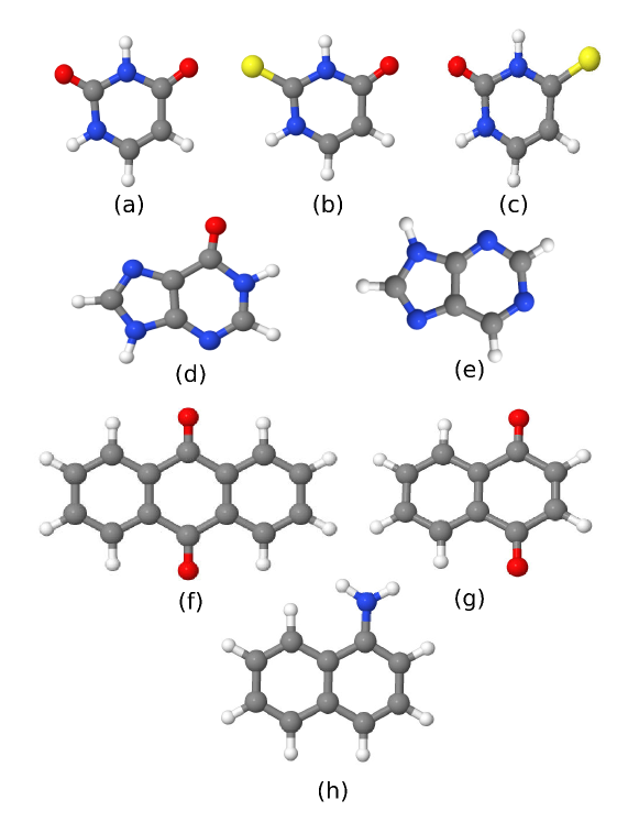
Figure 1: The molecules considered in this study: (a) uracil, (b) 2-thiouracil, (c) 4-thiouracil, (d) hypoxanthine, (e) purine, (f) 9,10-anthraquinone, (g) 1,4-naphthaquinone, (h) 1-naphthylamine.

Figure 2: The clusters with water considered in this study: (a) uracil + 4$\cdot$H₂O; (b) purine + 4$\cdot$H₂O, (c) hypoxanthine + 5$\cdot$H₂O.

The correlation-consistent aug-cc-pVDZ basis set Dunning Jr (1989) was used in the calculations of the $\mathcal{B}$ term. The RICC2 calculations were carried out with Turbomole. Balasubramani et al. (2020) In all calculations the gauge origin was placed in center of the nuclear charges. The convergence threshold for response equations was set equal to 10^-4 in all calculations. For ease of comparison with the experimental bands, we report in the tables the negative of the $\mathcal{B}$ term—according to the standard convention, a positive MCD band corresponds to a negative $\mathcal{B}$ term. Mason (2007) The OPA spectra are reported as decadic molar extinction coefficients $\epsilon(\omega)$ (in standard units M^-1cm^-1): Rizzo, Coriani, and Ruud (2012)

$$\epsilon(\omega)=703.301\times\omega\times\sum_{j}g(\omega,\omega_{j})\frac{3f_{j}}{2\omega_{j}}$$ (17)

where $\omega_{j}$ (in a.u.) and $f_{j}$ are the excitation energy and oscillator strength of electronic transition $j$, respectively, $\omega$ (in a.u.) is the frequency of the incoming radiation, and $g(\omega,\omega_{j})$ is a broadening function.

The MCD spectra are reported as extinction coefficient anisotropy, $\Delta\epsilon$ (in units M^-1cm^-1T^-1), which are connected to the $\mathcal{B}$ terms by Rizzo, Coriani, and Ruud (2012)

$$\Delta\epsilon=-\frac{8\pi^{2}N_{A}\omega{B}_{\textrm{ext}}}{3\times 1000\times\ln(10)(4\pi\epsilon_{0}\hbar c_{0})}\sum_{j}g(\omega,\omega_{j}){\mathcal{B}}(0\rightarrow{j}),$$ (18)

where ${B}_{\textrm{ext}}$ is the strength of external magnetic field, $\epsilon_{0}$ is the vacuum permittivity, and $N_{A}$ is Avogadro’s number. In both expressions, we use a Lorentzian broadening function

$$g(\omega,\omega_{j})=\frac{1}{\pi}\frac{\gamma}{(\omega-\omega_{j})^{2}+\gamma^{2}}\leavevmode\nobreak\ ,$$ (19)

with a half width at half maximum (HWHM) value of $\gamma\leavevmode\nobreak\ =\leavevmode\nobreak\ 0.0045563$ Hartree (1000 cm^-1), if not stated otherwise.

The discussion of the results in the following section is based on spectra shifted in order to realign with experiment. Details on the shifts applied are given in the figure captions. Tables of raw data (transition energies, oscillator strengths and ${\mathcal{B}}$ terms) are reported in the SI file.

IV Results and Discussion

IV.1 Uracil, 2-thiouracil, 4-thiouracil

Experimental OPA and MCD spectra of uracil and thiouracils in water were recorded by Voelter et al.; Voelter et al. (1968) and Igarashi-Yamamoto et al., Igarashi-Yamamoto et al. (1981) respectively.

A computational study of the MCD spectrum of uracil (and other molecules) was presented by Fahleson et al. Fahleson et al. (2015) at the TD-DFT level of theory. Results from simulations both in vacuo and in water solution were reported, the latter described using the polarizable continuum model (PCM) with explicit water molecules. A detailed computational investigation of OPA and MCD spectra of various thiouracils, including 2-thiuracil and 4-thiouracil, was carried out by Martinez-Fernandez et al., Martinez-Fernandez et al. (2017) also at the TD-DFT level in vacuo and in PCM/water.

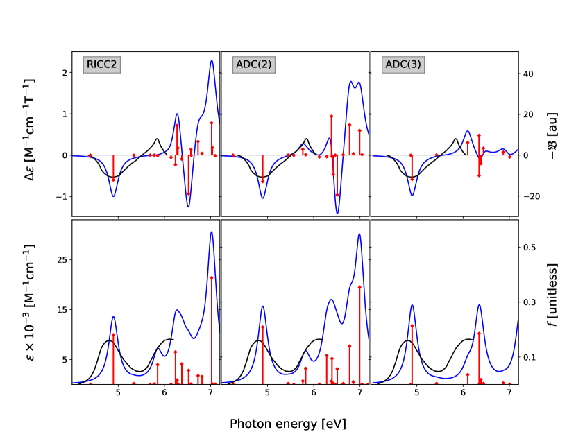
Figure 3: Uracil. MCD (upper panels) and OPA spectra (lower panels) at RICC2, ADC(2) and ADC(3) levels. The experimental spectra recorded in water (black lines) were digitized from Ref. 70. The simulated spectra were shifted to align with experiment by $-0.5$ eV (RICC2), $-0.4$ eV (ADC(2)) and $-0.45$ eV (ADC(3)).

Fig. 3, top panels, collects the MCD spectra computed at RICC2, ADC(2) and ADC(3) levels of theory. Fig. LABEL:SI-fig:Ur:2thio:4thio:ADC2x shows the spectra at the ADC(2)-x level. In the figures, we also report the experimental MCD spectrum of uracil (black line), recorded by Voelter et al. in water Voelter et al. (1968) in-between 4.5 eV (280 nm) and 6.0 eV (205 nm). This shows a negative band centered at around 4.9 eV (255 nm) and a positive one at around 5.8 eV (215 nm). The bottom panels show the OPA spectra, again with the black line as the experimental spectrum recorded in water, Voelter et al. (1968) which shows one well-separated feature centered at $\approx$4.8 eV (260 nm), plus the offset of a second peak.

Keeping in mind that the experimental spectra were recorded in water, whereas the calculations were done without solvent model, all simulated MCD spectra roughly reproduce the shape of the experimental spectrum. All methods attribute the first peak in both OPA and MCD to the bright $\pi\to\pi^{*}$ (1A’) excited state, well separated from the other excitations. The origin of the second feature, however, varies significantly between the four methods. In particular, ADC(2) and ADC(3) attribute it primarily to a transition to the 2A’ state, whereas in RICC2 the positive band comes from the balance between transitions of opposite signs, with 4A’ and 5A” as the main contributors. ADC(2)-x yields an almost negligible intensity of the second feature. Remarkably, the ADC(2) spectrum presents two positive bands in the mid-region (in between 5.5 eV–6.5 eV in the shifted spectrum in Fig. 3). However, as it can be seen from Fig. 4, when including four molecules (corresponding to the first solvation shell), using the optimized configuration of Ref. 66, the additional peak disappears and the agreement with experiment improves.

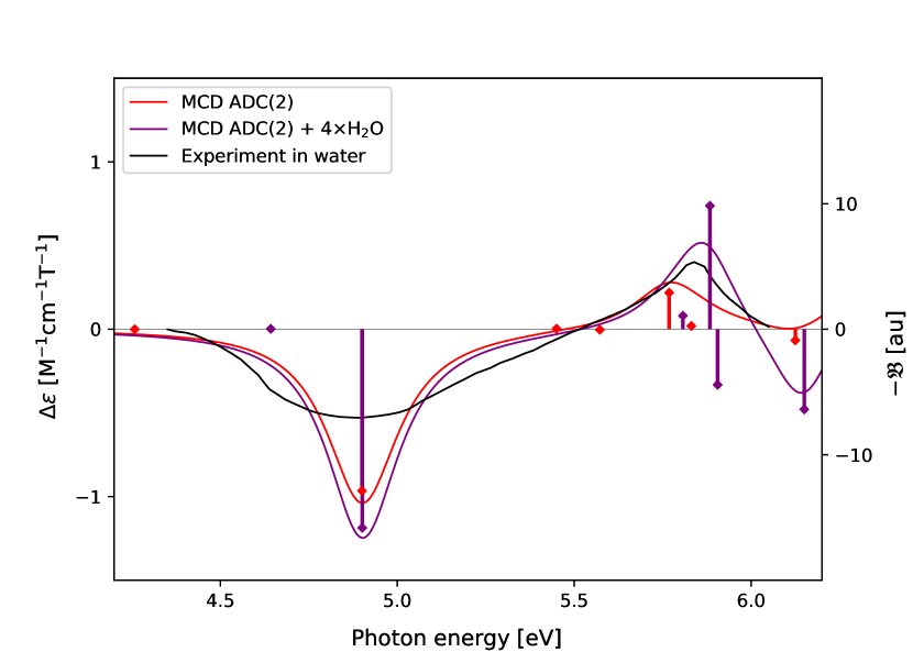
Figure 4: Uracil. Comparison of MCD at ADC(2) level in gas phase and for a model system including 4 explicit water molecules. The geometry of the latter was taken from Ref. 66. The experimental spectrum recorded in water Voelter et al. (1968) is also given. The computed spectra were shifted to align with the lowest energy experimental band, by $-0.4$ eV and $-0.25$ eV for gas phase and explicit solvation model, respectively.

In the experiment, the separation between the first and second band is $\sim$0.94 eV. Among the four computational methods, RICC2 yields (in vacuo) the largest separation, $\sim$1.4 eV while ADC(2)-x predicts the smallest one, around 0.6 eV. The ADC(2) method estimates this separation to be $\sim$0.87 eV and ADC(3) predicts a distance between the first and second feature of approximately 1.2 eV. The ADC(2) calculation with four explicit solvent molecules yields a peak separation of 1 eV, which is the result closest to experiment. Thus, explicit solvation slightly improves the relative distance between first and second peak of uracil, at least at ADC(2) level. Our attempts to cover a larger region were not successful due to convergence problems in the response equations for a higher number of roots.

Comparing to the TD-DFT Fahleson et al. (2015) results in vacuo and in water solution reported in Ref. 66, the TD-CAM-B3LYP Fahleson et al. (2015) spectrum is in agreement with all the ADC spectra, as well as the RICC2 ones. TD-B3LYP, on the other hand, shows a second negative feature at around 6.2 eV not present in the experimental spectrum (in solution). For both ADC(2) and TD-DFT, Fahleson et al. (2015)explicit consideration of a few water molecules improves the agreement with experiment.

Fig. 5 show the computed OPA and MCD spectra of 2-thiouracil. The experimental MCD spectrum, recorded in water, Igarashi-Yamamoto et al. (1981) covers the region from $\sim$3.8 eV (325 nm) to $\sim$5.5 eV (225 nm) and shows a very distinctive bisignate feature, with negative and positive lobes peaking at $\sim$4.3 eV (290 nm) and $\sim$4.7 eV, (263 nm), respectively. A third (negative) band of lower intensity is peaked at 5.2 eV (237 nm). Due to molecular symmetry, the bisignate MCD band is not attributable to an $\mathcal{A}$ term. It corresponds to a broad peak centered at around 4.5 eV in the experimental OPA spectrum, Igarashi-Yamamoto et al. (1981) revealing that more than one excited state contributes to the OPA band. The third, low intensity, MCD peak also appears to correspond to a transition ’hidden’ between the first broad OPA band and the second OPA peak emerging at around 6.2 eV. In the experimental study, the MCD spectrum was interpreted based on the hypothesis that a tautomeric equilibrium exists between thiol and thione forms of 2-thiouracil in solution. Thus, the band at 290 nm was tentatively assigned to a thiol form, and the one at $\approx$270 nm to a thione form. Another possibility to elucidate the spectrum mentioned in the experimental study is that the two peaks are due to two “local” $\pi\pi^{*}$ transitions, one on the thiourea moiety and one on the acrolein moiety. This interpretation was disregarded as too difficult to verify experimentally.

All four methods reproduce the bisignate feature observed in the experimental spectrum, and confirm the presence of two electronic excitations within the first OPA band. Also, all methods indicate the presence of an additional negative band moving towards higher energies, which contains contributions from several excited states. Inspection of the natural transition orbitals (NTOs) for the two dominant excitations (see Figure LABEL:SI-fig:2-thio:NTOs) reveals that the first (negative) MCD band is a $\pi\pi^{*}$ where $\pi^{*}$ involves the S atom, whereas the transition responsible for the positive band is a $\pi\pi^{*}$ one, where $\pi^{*}$ involves the C=O group. This seems to support the second interpretation of the origin of the bisignate feature.

As observed for uracil, the high energy region of the spectra shows remarkably different MCD patterns between the four methods, and we refrain from a detailed discussion, also because the experimentally recorded spectra do not extend in such region.

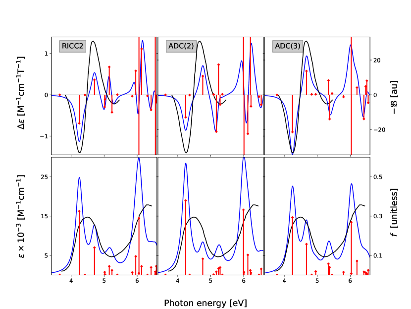
Figure 5: 2-thiouracil. MCD (upper panels) and OPA spectra (lower panels) at RICC2, ADC(2) and ADC(3) levels. The experimental spectra recorded in water, shown as black lines, were digitized from Ref.71 and rescaled following Ref. 72. The simulated spectra were shifted to align with experiment, by $-0.38$ eV (RICC2), $-0.23$ eV (ADC(2)) and $-0.38$ eV (ADC(3)).

Similar to the TD-DFT Martinez-Fernandez et al. (2017) results, in gas-phase the computed intensities are smaller than the experimental ones, except for those yielded by the ADC(3) method. ADC(3) provides an almost identical intensity for the first band and a small underestimation of the second one.

The results at the RICC2, ADC(2) and ADC(3) levels of theory for 4-thiouracil are shown in Fig. 6. The ADC(2)-x spectra are in the SI. The spectral profiles are distinctively different from those of 2-thiouracil, highlighting the ability of MCD spectroscopy to discriminate between the two thiouracil isomers, as well as from uracil. The lower-energy region of the MCD spectrum of 4-thiouracil presents two negative bands ($\sim$3.8 eV and $\sim$4.8) and a positive one at around 5.5 eV. The overall intensity of the MCD spectrum is, according to the experiment, Igarashi-Yamamoto et al. (1981) weaker than in 2-thiouracil. Both trends are reproduced in our calculations, even though for ADC(2)-x and ADC(3) the second negative band is as intense or even more intense than the first band. One should keep in mind, however, that the experiment was recorded in water, so the comparison between theory and experiment can only be qualitative. For all four methods, the first negative band is attributed to one, well-separated, electronic transition, whereas several transitions may be contributing to the second band.

Moving towards higher energies, the experimental and simulated spectra deviate from each other. As before, we do not discuss this region, as solvent effects are not accounted for in the computed spectra.

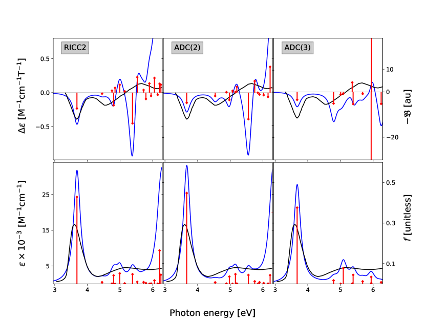
Figure 6: 4-thiouracil. MCD (upper panels) and OPA spectra (lower panels) for RICC2, ADC(2) and ADC(3). Experimental spectra recorded in water are presented as black solid lines. The simulated spectra were shifted to align with experiment by $-0.6$ eV (RICC2), $-0.38$ eV (ADC(2)) and $-0.34$ eV (ADC(3)). The experimental spectra were digitized from Ref.71 and rescaled as in Ref. 72. All three methods also yield a low-energy dark transition, which (once shifted) falls outside the frequency range in the figures.

IV.2 Purine and hypoxanthine

The OPA and MCD spectra of purine were recorded by Djerassi, Bunnenberg, and ElderDjerassi, Bunnenberg, and Elder (1971) in water. A computational investigation at the TD-DFT level both in vacuo and using explicit and implicit solvation models was presented in Ref. 66. Purine was also studied at the CC2 and CCSD level in vacuo and using COSMO in Ref. 24. Experimental spectra data of the purine derivative hypoxanthine have been presented in water by Sutherland and GriffinSutherland and Griffin (1984) and by Voelter et al. Voelter et al. (1968) Hypoxanthine was the subject of computation analysis in Ref. 75 at the Polarizable-Embedding TD-DFT level, and also at TD-DFT level using the polarizable continuum model (PCM) with and without explicit water molecules in Ref. 66. Our computed spectra at RICC2, ADC(2) and ADC(3) level in vacuo for both molecules are presented in Figs. 7 and 9. Fig. LABEL:SI-fig:Pur:Hypo:ADC2-x shows the ADC(2)-x spectra.

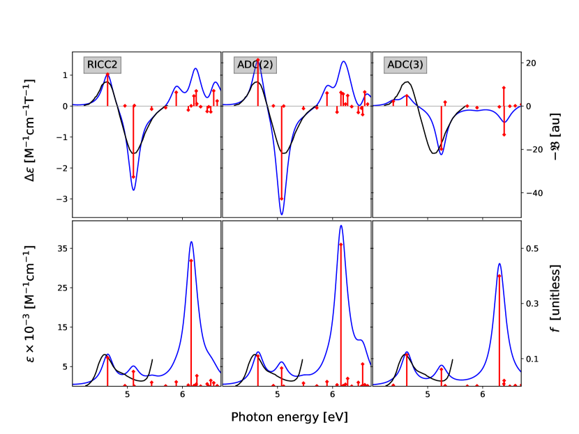
Figure 7: Purine. MCD (upper panels) and OPA (lower panels) at RICC2 and ADC(2) level. Experimental spectra recorded in water are presented as black lines, and were digitized from Ref.73. The simulated spectra were shifted to align with experiment by $-0.54$ eV (RICC2), $-0.51$ eV (ADC(2)) and $-0.34$ eV (ADC(3)). We note that ADC(2) and RICC2 also predict a low-energy optically dark transition (located at $\sim$3.9 eV after shifting), which falls outside the frequency range plotted.

The experimental MCD spectrum of purine is characterized by a bisignate feature with the positive lobe in the low energy region. Both RICC2 and ADC(2) attribute this lowest energy peak to a single excited state state (1A’) with negative $\mathcal{B}$ term, whereas the negative lobe is due to the fourth excited state (2A’) having a positive $\mathcal{B}$ term (For both methods, the first, optically dark state, falls outside the figures range). For ADC(3), both the first (1A”) and the second (1A’) electronic excited states contribute to the first MCD band, even though the first excitation is practically dark in OPA. In ADC(2)-x the fifth excited state is responsible for the negative MCD lobe (also in this case there is a first optically dark state outside the figures range). The larger intensity of the second peak over the first one is reproduced by all four methods. In the high energy region, RICC2 and ADC(2) predict several positive features, due to multiple transitions, while ADC(2)-x predicts only one. In contrast to the other methods, ADC(3) predicts a negatively signed third band. Note that the experimental spectrum does not reach this region.

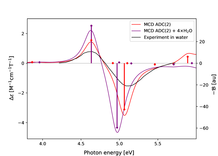
Figure 8: Purine. Comparison of MCD spectra at ADC(2) level in vacuo and for a model system including 4 explicit water molecules. The geometry of the latter was taken from Ref. 66. The experimental spectrum was digitized from Ref.73. The simulated spectra were shifted by $-0.5$ eV (gas phase) and $-0.56$ eV (explicit solvation model) to align them to the inflection point in the experiment.

For purine, the importance of solvent effects is illustrated, at ADC(2) level, in Fig. 8. Including the first solvation shell in the calculations increases the intensity of both features by approximately a factor of two and reduces the separation between the two bands, deteriorating the agreement with the experiment. We also refer to the study by Khani et al.Khani et al. (2018) for a discussion of solvent effects on the MCD spectrum of purine via COSMO.

The spectra of hypoxanthine are presented in Fig. 9. The experimental MCD spectrum (once again in water) shows two bisignate features in-between 4.4–6.9 eV. All methods reproduce the first “pseudo-$\mathcal{A}$” band, due to the 1A’ and 2A’ states; the ADC methods struggle with the one at higher energy, in particular to reproduce the positive lobe. According to RICC2, the fourth spectral feature is due to two close-lying transitions (11A’ and 12A”). In contrast, ADC(2) predicts two low-intensity positive peaks, formed by many transitions with $\mathcal{B}$ terms of different sign and intensity. As we are reaching higher energies, where many transitions contribute to the OPA and MCD bands, the stick-spectrum approach may become inefficient, due to the increasing number of excited states to be converged. In support of our statement, we note that in the TD-DFT study reported by Fahleson et al.Fahleson et al. (2015) using the complex-polarization-propagator approach, where the MCD signal is directly computed, the second bisignate feature is indeed well reproduced.

The ADC(2) simulation using the explicit solvation model for hypoxanthine (Fig. 10) reproduces the first and the second spectral features with slightly larger intensities. As in the analogous calculation for purine, the separation between the bright states becomes smaller, which, in this specific case, does improve a bit the agreement with the experiment.

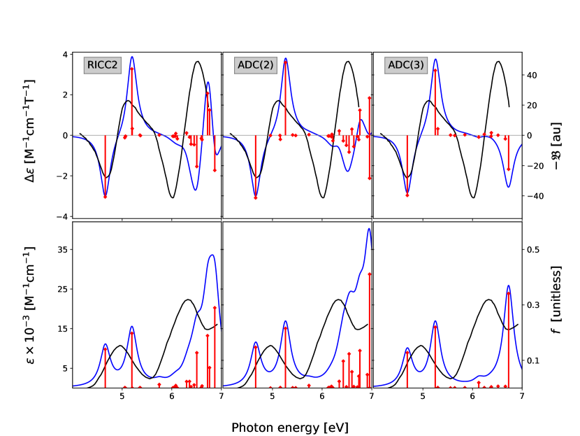
Figure 9: Hypoxanthine. MCD (upper panels) and OPA (lower panels) at RICC2 and ADC(2) levels. The experimental spectra recorded in water (black lines) were digitized from Ref.74. The simulated spectra were shifted to align with experiment: –0.39 eV, –0.26 eV and –0.22 eV for RICC2, ADC(2) and ADC(3) respectively.

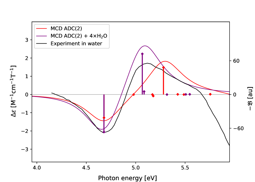
Figure 10: Hypoxanthine. Comparison of MCD spectra at ADC(2) level in vacuo and for a model system including 5 explicit water molecules, whose geometry was taken from Ref. 66. The experimental spectrum was digitized from Ref.74. The simulated spectra were shifted to align them with the experimental inflection point at lowest energy, by $-$0.24 eV (gas) and $-$0.28 eV (solvated), respectively. The $\gamma$ parameter (see Eq. 19) for this figure is 8.56 $\times$10^-3 a.u.

IV.3 1,4-naphthoquinone, 9,10-anthraquinone and 1-naphthylamine

As final examples, we considered two quinones, the smaller 1,4-naphthoquinone (NQ) and the larger 9,10-anthraquinone (AQ), and 1-naphthylamine (1NA). Experimental MCD spectra for NQ and AQ were reported, together with those for other ketones, by Meier and WagnièreMeier and Wagnière (1987) and Dearman.Dearman (1973) These results have earlier provided a reference for theoretical investigations at different levels of theory.Coriani et al. (2000); Meier and Wagnière (1987); Fukuda et al. (1983); Dearman (1973); Sun et al. (2019); Seth et al. (2008a) A TD-DFT study,Seth et al. (2008a) in particular, showed contradictory results with respect to the experimental data, which makes NQ and AQ interesting test cases for our MCD-ADC scheme. Given the size of NQ and AQ, only RICC2 and ADC(2) are considered.

As in Ref. 18, we do not discuss the lowest energy transitions in NQ, which Meier and WagnièreMeier and Wagnière (1987) attributed to n$\pi^{*}$. Simulations of the MCD spectrum for NQ were reported by Seth et al. Seth et al. (2008a) at TD-DFT level, and by Sun et al. Sun et al. (2019) using real-time (RT-) TD-DFT (B3LYP functional) and gauge-including atomic orbitals (6-31G(d) basis set). The experimental spectrum of NQ includes three well-distinguishable features: a low-intensity pseudo-$\mathcal{A}$ feature with inflection point at $\sim$3.8 eV, a positive peak at around 4.9 eV, followed by a series of well-defined negative peaks of progressively increasing intensities. Both ADC(2) and RICC2 reproduce the two first experimental features, though with higher intensities. In correspondence to the positive band at around 5.1 eV, RICC2 shows a numerical instability, as two degenerate transitions with exceedingly large and oppositely signed ${\mathcal{B}}$ terms are obtained. Closer analysis reveals that the RICC2 results for the excitation energies of 1,4-naphthoquinone are quite sensitive to the geometry used in the calculations. In the high energy region, ADC(2) and RICC2 both predict a strong positive peak (due to the 6B₁ transition) at around 6.5 eV, not present in the experimental spectrum (recorded in cyclohexane). The spectra available at TD-DFT level are also in qualitative agreement with the experimental spectral profile of NQ. However, in the spectrum reported by Sun et al. Sun et al. (2019) the relative intensity of the negative peaks is off compared to experiment. The SAOP/QZ3P1D and BP86/DZP spectra reported by Seth et al., Seth et al. (2008a) on the other hand, present a much better agreement of the relative intensities of these two negative bands. BP86/DZP fails in yielding the negative lobe of the low-energy bisignate band of NQ.

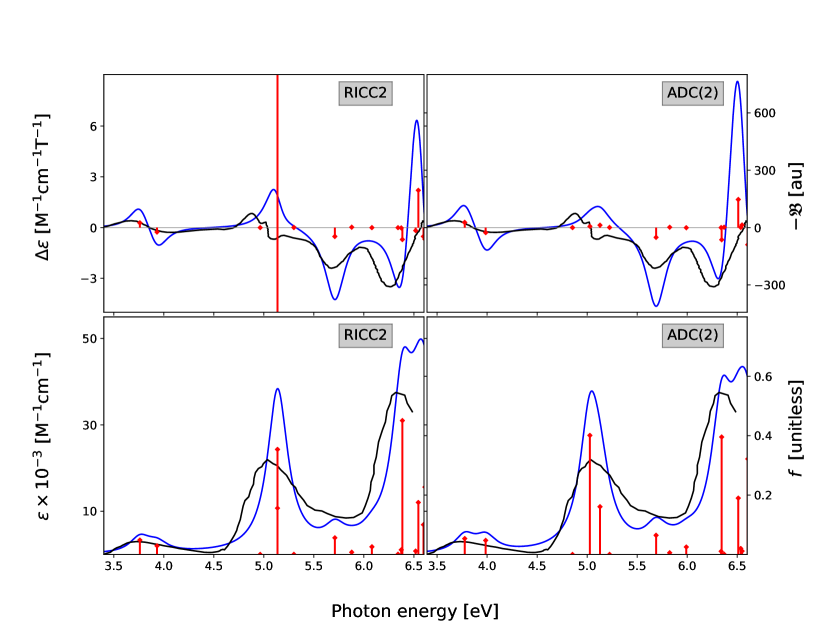
Figure 11: 1,4-naphthoquinone (NQ). MCD (upper panels) and OPA spectra (lower panels) at RICC2 and ADC(2) level. Experimental spectra recorded in cyclohexane (black lines) were digitized from Ref.76 and scaled by 10⁴. The simulated spectra were shifted by $-$0.39 eV (RICC2) and $-$0.38 eV (ADC(2)) to align with experiment. Only one of the two dark transitions [at $\sim$2.81 eV (440 nm) and 2.72 eV (455 nm)], predicted in Ref. 76, was found at $\sim$2.5 eV (ADC(2)) and $\sim$2.6 eV (RICC2) after shifting. This dark transition is not shown.

The experimental spectrum of AQ presents two positive features in the low-energy region, located at $\sim$3.85 eV and at $\sim$4.6 eV, followed by a relatively intense pseudo-$\mathcal{A}$ band in between 4.6 and 5.6 eV. Both SAOP/QZ3P1D and BP86/DZP TD-DFT calculations Seth et al. (2008a) reproduce the first feature in the low-energy part of the spectrum. However, they both predict an opposite sign pattern with respect to the experiment for the pseudo-$\mathcal{A}$ band. In contrast, RICC2 and ADC(2) yield the correct sign pattern of the intense pseudo-$\mathcal{A}$ band, with positive and negative lobes due to the 2B_3u and 2B_2u transitions, respectively. They also reproduce the first weak feature, though shifted (it is located at $\sim$3.9 eV after the overall realignment with experiment). Both second-order methods fail to predict sign and intensity of the feature around 4.6 eV: for RICC2 this transition is basically dark to MCD, while for ADC(2) it is negative (it has a small positive $\mathcal{B}$). From the results reported in Ref. 18, we could not discern whether this feature was reproduced or not by the SAOP/QZ3P1D and BP86/DZ methods. Thus, none of the simulated MCD spectra is fully consistent with the experimental MCD spectrum of AQ. Nonetheless, both RICC2 and ADC(2) reproduce the most important spectral features of AQ.

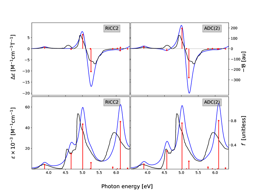
Figure 12: 9,10-anthraquinone (AQ). MCD (upper panels) and OPA spectra (lower panels) at the RICC2 and ADC(2) level. Experimental spectra recorded in cyclohexane are presented as black lines, digitized from Ref.76 and scaled by 10⁴. The simulated spectra were shifted by $-$0.46 eV to align with the inflection point of the pseudo-$\mathcal{A}$ band in the experiment. None of the two dark transitions (at around 3.31 eV (375 nm) and 2.95 eV (420 nm)) otherwise predicted in Ref. 76, was found.

The experimental MCD spectrum of 1NA was recorded in cyclohexane by Whipple, Vasak, and Michl. Whipple, Vasak, and Michl (1978) It includes a bisignate feature in the low-energy region of the spectrum and two negative peaks in the region $\sim$3.4-6 eV. A computational study at the RICC2, TD-B3LYP and TD-CAM-B3LYP levels of theory was recently reported by Ghidinelli et al. Ghidinelli et al. (2020) Ghidinelli et al. noted that RICC2 and TD-CAM-B3LYP methods well reproduced the profile of the experimental spectrum, while TD-B3LYP yielded a small positive peak in-between the two negative features in the high-energy region. Close inspection of our results reveals very similar results for RICC2 and ADC(2), though one of the negative $\mathcal{B}$ terms in the region around $\sim$6.1 eV is slightly larger for ADC(2) than RICC2. If a $\gamma$ value of 1000 cm^-1 is used for the broadening, this results in the emergence of a small positive band for ADC(2), like it was observed for TD-B3LYP.Ghidinelli et al. (2020) One should not forget, however, that the appearance of the spectrum depends on the chosen value of the broadening. Adjusting $\gamma$ to 5.7$\times$10^-3 a.u., the broadened ADC(2) spectrum becomes fully consistent with the RICC2 one. For both second-order methods, the bisignate feature is due to the $L_{a}$ and $L_{b}$ transitions: 1A’ (negative band) and 2A’ (positive band). Several transitions, most of them of relatively low-intensity contribute to the first negative band, while the second one is, in both methods, due to the 7A’ transition.

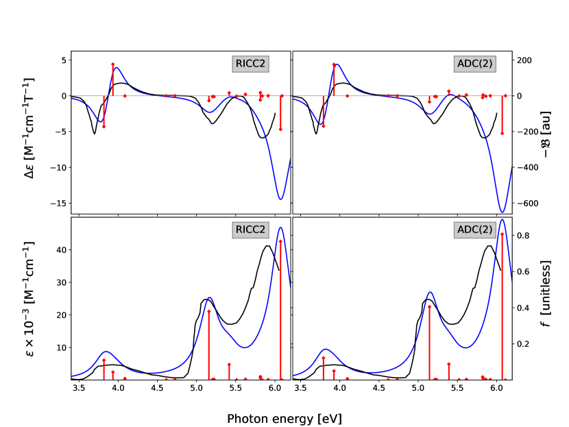
Figure 13: 1-Naphthylamine (1N). MCD (upper panels) and OPA spectra (lower panels) at RICC2 and ADC(2) level. Experimental spectrum, recorded in cyclohexane, is presented as black lines, digitized from Ref.80. Both simulated spectra were shifted by $-$0.17 eV to align with the lower-energy experimental inflection point. Here, $\gamma$ = 5.7$\times$10^-3 a.u. was used.

V Conclusions

We have presented the derivation and implementation of a computational scheme for the $\mathcal{B}$ term of Magnetic Circular Dichroism within the ADC/ISR framework, thus extending the pool of spectroscopic effects that can be simulated using the ADC($n$) methods. In the lowest-energy region of the spectra, an overall qualitative agreement with experiment is observed for all ADC methods. Modelling the higher energy region with the presented approach is more demanding as the density of electronic states increases and a large number of converged states is required. An alternative ansatz is offered by the complex-polarization propagator approach which is more suited for that situation. Work in this direction is currently ongoing.

Supplementary Material

Tables of raw spectral data (energies, oscillator strengths and (negative) ${\mathcal{B}}$ terms; ADC(2)-x spectra; ADC(2) natural transition orbitals of the first two MCD bands in 2-thiouracil; Cartesian coordinates of all molecules.

Author declarations

Conflict of Interest

The authors have no conflicts to disclose.

Author contributions

S. C. and A. D. conceptualized and supervised the project. D. A. F., M. S. and D. R. R. derived the working equations and implemented the computational methodology. D. A. F. performed the calculations. D. A. F. and S. C. drafted the manuscript. All authors revised the draft and discussed its scientific content.

Data Availability

The data that supports the findings of this study are available within the article and its supplementary material.

References

- Buckingham and Stephens (1966) A. D. Buckingham and P. J. Stephens, “Magnetic Optical Activity,” Annu. Rev. Phys. Chem. 17, 399–432 (1966).
- Barron (2004) L. D. Barron, Molecular light scattering and optical activity. Second Edition (Cambridge University Press, Cambridge, UK, 2004).
- Cukras et al. (2016) J. Cukras, J. Kauczor, P. Norman, A. Rizzo, G. L. J. A. Rikken, and S. Coriani, “A complex-polarization-propagator protocol for magneto-chiral axial dichroism and birefringence dispersion,” Phys. Chem. Chem. Phys. 18, 13267–13279 (2016).
- Serber (1932) R. Serber, “The Theory of the Faraday Effect in Molecules,” Phys. Rev. 41, 489–506 (1932).
- Stephens (1970) P. J. Stephens, “Theory of Magnetic Circular Dichroism,” J. Chem. Phys. 52, 3489–3516 (1970).
- Stephens (1974) P. J. Stephens, “Magnetic Circular Dichroism,” Annu. Rev. Phys. Chem. 25, 201–232 (1974).
- Stephens (1976) P. J. Stephens, “Magnetic Circular Dichroism,” in Adv. Chem. Phys. (John Wiley & Sons, Ltd, 1976) pp. 197–264.
- Mason (2007) W. R. Mason, A practical guide to magnetic circular dichroism spectroscopy (Wiley-Interscience, 2007).
- Sutherland and Holmquist (1980) J. C. Sutherland and B. Holmquist, “Magnetic circular dichroism of biological molecules,” Annu. Rev. Biophys. Bioeng 9, 293–326 (1980).
- Kjærgaard, Coriani, and Ruud (2012) T. Kjærgaard, S. Coriani, and K. Ruud, “Ab initio calculation of magnetic circular dichroism,” Wiley Interdisciplinary Reviews: Computational Molecular Science 2, 443–455 (2012).
- Shieh, Lin, and Eyring (1972) D. J. Shieh, S. H. Lin, and H. Eyring, “Magnetic circular dichroism of molecules in dense media. I. Theory,” J. Phys. Chem. 76, 1844–1848 (1972).
- Miles and Eyring (1973) D. W. Miles and H. Eyring, “Molecular orbital calculations of magnetic circular dichroism spectra: A benzene-indole sequence,” Proc. Natl. Acad. Sci. 70, 3754–3758 (1973).
- Goldstein, Vijaya, and Segal (1980) E. Goldstein, S. Vijaya, and G. A. Segal, “Theoretical study of the optical absorption and magnetic circular dichroism spectra of cyclopropane,” J. Am. Chem. Soc. 102, 6198–6204 (1980).
- Warnick and Michl (1974) S. M. Warnick and J. Michl, “Use of semiempirical models for calculation of B terms in MCD [magnetic circular dichroism] spectra. I. General results and the Pariser-Parr-Pople (PPP) model for nonalternant hydrocarbons,” J. Am. Chem. Soc. 96, 6280–6289 (1974).
- Olsen and Jørgensen (1985) J. Olsen and P. Jørgensen, “Linear and nonlinear response functions for an exact state and for an MCSCF state,” J. Chem. Phys. 82, 3235 (1985).
- Coriani et al. (1999) S. Coriani, P. Jørgensen, A. Rizzo, K. Ruud, and J. Olsen, “Ab initio determinations of magnetic circular dichroism,” Chem. Phys. Lett. 300, 61–68 (1999).
- Seth et al. (2004) M. Seth, T. Ziegler, A. Banerjee, J. Autschbach, S. J. A. van Gisbergen, and E. J. Baerends, “Calculation of the Term of Magnetic Circular Dichroism based on Time Dependent-Density Functional Theory I. Formulation and Implementation,” J. Chem. Phys. 120, 10942–10954 (2004).
- Seth et al. (2008a) M. Seth, M. Krykunov, T. Ziegler, J. Autschbach, and A. Banerjee, “Application of Magnetically Perturbed Time-Dependent Density Functional Theory to Magnetic Circular Dichroism: Calculation of Terms,” J. Chem. Phys. 128, 144105 (2008a).
- Seth et al. (2008b) M. Seth, M. Krykunov, T. Ziegler, and J. Autschbach, “Application of Magnetically Perturbed Time-Dependent Density Functional Theory to Magnetic Circular Dichroism. II. Calculation of Terms,” J. Chem. Phys. 128, 234102 (2008b).
- Solheim et al. (2008a) H. Solheim, L. Frediani, K. Ruud, and S. Coriani, “An IEF-PCM Study of Solvent Effects on the Faraday B Term of MCD,” Theor. Chem. Acc. 119, 231–244 (2008a).
- Seth and Ziegler (2010) M. Seth and T. Ziegler, “Calculation of Magnetic Circular Dichroism Spectra With Time-Dependent Density Functional Theory,” Advances in Inorganic Chemistry 62, 41–109 (2010).
- Kjærgaard et al. (2009) T. Kjærgaard, P. Jørgensen, A. J. Thorvaldsen, P. Sałek, and S. Coriani, “Gauge-Origin Independent Formulation and Implementation of Magneto-Optical Activity within Atomic-Orbital-Density Based Hartree- Fock and Kohn- Sham Response Theories,” J. Chem. Theory Comput. 5, 1997–2020 (2009).
- Coriani et al. (2000) S. Coriani, C. Hättig, P. Jørgensen, and T. Helgaker, “Gauge-origin independent magneto-optical activity within coupled cluster response theory,” J. Chem. Phys. 113, 3561–3572 (2000).
- Khani et al. (2018) S. K. Khani, R. Faber, F. Santoro, C. Hättig, and S. Coriani, “UV absorption and magnetic circular dichroism spectra of purine, adenine, and guanine: A coupled cluster study in vacuo and in aqueous solution,” J. Chem. Theory Comput. 15, 1242–1254 (2018).
- Faber et al. (2020) R. Faber, S. Ghidinelli, C. Hättig, and S. Coriani, “Magnetic circular dichroism spectra from resonant and damped coupled cluster response theory,” J. Chem. Phys. 153, 114105 (2020).
- Norman et al. (2001) P. Norman, D. M. Bishop, H. J. A. Jensen, and J. Oddershede, “Near-resonant absorption in the time-dependent self-consistent field and multiconfigurational self-consistent field approximations,” J. Chem. Phys. 115, 10323–10334 (2001).
- Norman (2011) P. Norman, “A perspective on nonresonant and resonant electronic response theory for time-dependent molecular properties,” Phys. Chem. Chem. Phys. 13, 20519–20535 (2011).
- Krykunov et al. (2007) M. Krykunov, M. Seth, T. Ziegler, and J. Autschbach, “Calculation of the Magnetic Circular Dichroism B Term from the Imaginary Part of the Verdet Constant using Damped Time-Dependent Density Functional Theory,” J. Chem. Phys. 127, 244102 (2007).
- Solheim et al. (2008b) H. Solheim, K. Ruud, S. Coriani, and P. Norman, “Complex polarization propagator calculations of magnetic circular dichroism spectra,” J Chem. Phys. 128, 094103 (2008b).
- Ganyushin and Neese (2008) D. Ganyushin and F. Neese, “First-principles calculations of magnetic circular dichroism spectra,” J. Chem. Phys. 128, 114117 (2008).
- Lee, Yabana, and Bertsch (2011) K.-M. Lee, K. Yabana, and G. F. Bertsch, “Magnetic circular dichroism in real-time time-dependent density functional theory,” J. Chem. Phys. 134, 144106 (2011).
- Sun et al. (2019) S. Sun, R. A. Beck, D. Williams-Young, and X. Li, “Simulating Magnetic Circular Dichroism Spectra with Real-Time Time-Dependent Density Functional Theory in Gauge Including Atomic Orbitals,” J. Chem. Theory Comput. 15, 6824–6831 (2019).
- Wormit et al. (2014) M. Wormit, D. R. Rehn, P. H. Harbach, J. Wenzel, C. M. Krauter, E. Epifanovsky, and A. Dreuw, “Investigating excited electronic states using the algebraic diagrammatic construction (ADC) approach of the polarisation propagator,” Mol. Phys. 112, 774–784 (2014).
- Schirmer (1982) J. Schirmer, “Beyond the random-phase approximation: A new approximation scheme for the polarization propagator,” Phys. Rev. A 26, 2395 (1982).
- Trofimov, Stelter, and Schirmer (1999) A. B. Trofimov, G. Stelter, and J. Schirmer, “A consistent third-order propagator method for electronic excitation,” J. Chem. Phys. 111, 9982–9999 (1999).
- Trofimov, Stelter, and Schirmer (2002) A. B. Trofimov, G. Stelter, and J. Schirmer, “Electron excitation energies using a consistent third-order propagator approach: Comparison with full configuration interaction and coupled cluster results,” J. Chem. Phys. 117, 6402–6410 (2002).
- Trofimov and Schirmer (2005) A. B. Trofimov and J. Schirmer, “Molecular ionization energies and ground- and ionic-state properties using a non-dyson electron propagator approach,” J. Chem. Phys. 123, 144115 (2005).
- Handke et al. (1995) G. Handke, F. Tarantelli, A. Tarantelli, and L. Cederbaum, “The ab initio calculation of very many triply ionized states of molecular systems,” J. Electr. Spectros. Rel. Phenom. 75, 109–115 (1995).
- Barth and Schirmer (1985) A. Barth and J. Schirmer, “Theoretical core-level excitation spectra of N2 and CO by a new polarisation propagator method,” J. Phys. B: At. Mol. Phys. 18, 867–885 (1985).
- Plekan et al. (2008) O. Plekan, V. Feyer, R. Richter, M. Coreno, M. de Simone, K. Prince, A. Trofimov, E. Gromov, I. Zaytseva, and J. Schirmer, “A theoretical and experimental study of the near edge X-ray absorption fine structure (NEXAFS) and X-ray photoelectron spectra (XPS) of nucleobases: Thymine and adenine,” Chem. Phys. 347, 360–375 (2008).
- Trofimov et al. (2000) A. Trofimov, T. E. Moskovskaya, E. V. Gromov, N. M. Vitkovskaya, and J. Schirmer, “Core-level electronic spectra in ADC(2) approximation for polarization propagator: carbon monoxyde and nitrogen molecules,” J. Struct. Chem. 41, 483–494 (2000).
- Wenzel et al. (2015) J. Wenzel, A. Holzer, M. Wormit, and A. Dreuw, “Analysis and comparison of cvs-adc approaches up to third order for the calculation of core-excited states,” J. Chem. Phys. 142, 214104 (2015).
- Schirmer (1991) J. Schirmer, “Closed-form intermediate representations of many-body propagators and resolvent matrices,” Phys. Rev. A 43, 4647–4659 (1991).
- Schirmer and Trofimov (2004) J. Schirmer and A. Trofimov, “Intermediate state representation approach to physical properties of electronically excited molecules,” J. Chem. Phys. 120, 11449–11464 (2004).
- Fransson and Dreuw (2018) T. Fransson and A. Dreuw, “Simulating x-ray emission spectroscopy with algebraic diagrammatic construction schemes for the polarization propagator,” J. Chem. Theory Comput. 15, 546–556 (2018).
- Harbach, Wormit, and Dreuw (2014) P. H. P. Harbach, M. Wormit, and A. Dreuw, “The third-order algebraic diagrammatic construction method (ADC (3)) for the polarization propagator for closed-shell molecules: Efficient implementation and benchmarking,” J. Chem. Phys. 141, 064113 (2014).
- Shao et al. (2015) Y. Shao, Z. Gan, E. Epifanovsky, A. T. Gilbert, M. Wormit, J. Kussmann, A. W. Lange, A. Behn, J. Deng, X. Feng, D. Ghosh, M. Goldey, P. R. Horn, L. D. Jacobson, I. Kaliman, R. Z. Khaliullin, T. Kuś, A. Landau, J. Liu, E. I. Proynov, Y. M. Rhee, R. M. Richard, M. A. Rohrdanz, R. P. Steele, E. J. Sundstrom, H. L. Woodcock III, P. M. Zimmerman, D. Zuev, B. Albrecht, E. Alguire, B. Austin, G. J. O. Beran, Y. A. Bernard, E. Berquist, K. Brandhorst, K. B. Bravaya, S. T. Brown, D. Casanova, C.-M. Chang, Y. Chen, S. H. Chien, K. D. Closser, D. L. Crittenden, M. Diedenhofen, R. A. DiStasio Jr., H. Do, A. D. Dutoi, R. G. Edgar, S. Fatehi, L. Fusti-Molnar, A. Ghysels, A. Golubeva-Zadorozhnaya, J. Gomes, M. W. Hanson-Heine, P. H. Harbach, A. W. Hauser, E. G. Hohenstein, Z. C. Holden, T.-C. Jagau, H. Ji, B. Kaduk, K. Khistyaev, J. Kim, J. Kim, R. A. King, P. Klunzinger, D. Kosenkov, T. Kowalczyk, C. M. Krauter, K. U. Lao, A. D. Laurent, K. V. Lawler, S. V. Levchenko, C. Y. Lin, F. Liu, E. Livshits, R. C. Lochan, A. Luenser, P. Manohar, S. F. Manzer, S.-P. Mao, N. Mardirossian, A. V. Marenich, S. A. Maurer, N. J. Mayhall, E. Neuscamman, C. M. Oana, R. Olivares-Amaya, D. P. O’Neill, J. A. Parkhill, T. M. Perrine, R. Peverati, A. Prociuk, D. R. Rehn, E. Rosta, N. J. Russ, S. M. Sharada, S. Sharma, D. W. Small, A. Sodt, T. Stein, D. Stück, Y.-C. Su, A. J. Thom, T. Tsuchimochi, V. Vanovschi, L. Vogt, O. Vydrov, T. Wang, M. A. Watson, J. Wenzel, A. White, C. F. Williams, J. Yang, S. Yeganeh, S. R. Yost, Z.-Q. You, I. Y. Zhang, X. Zhang, Y. Zhao, B. R. Brooks, G. K. Chan, D. M. Chipman, C. J. Cramer, W. A. G. III, M. S. Gordon, W. J. Hehre, A. Klamt, H. F. S. III, M. W. Schmidt, C. D. Sherrill, D. G. Truhlar, A. Warshel, X. Xu, A. Aspuru-Guzik, R. Baer, A. T. Bell, N. A. Besley, J.-D. Chai, A. Dreuw, B. D. Dunietz, T. R. Furlani, S. R. Gwaltney, C.-P. Hsu, Y. Jung, J. Kong, D. S. Lambrecht, W. Liang, C. Ochsenfeld, V. A. Rassolov, L. V. Slipchenko, J. E. Subotnik, T. V. Voorhis, J. M. Herbert, A. I. Krylov, P. M. Gill, and M. Head-Gordon, “Advances in molecular quantum chemistry contained in the q-chem 4 program package,” Mol. Phys. 113, 184–215 (2015).
- Epifanovsky et al. (2021) E. Epifanovsky, A. T. B. Gilbert, X. Feng, J. Lee, Y. Mao, N. Mardirossian, P. Pokhilko, A. F. White, M. P. Coons, A. L. Dempwolff, Z. Gan, D. Hait, P. R. Horn, L. D. Jacobson, I. Kaliman, J. Kussmann, A. W. Lange, K. U. Lao, D. S. Levine, J. Liu, S. C. McKenzie, A. F. Morrison, K. D. Nanda, F. Plasser, D. R. Rehn, M. L. Vidal, Z.-Q. You, Y. Zhu, B. Alam, B. J. Albrecht, A. Aldossary, E. Alguire, J. H. Andersen, V. Athavale, D. Barton, K. Begam, A. Behn, N. Bellonzi, Y. A. Bernard, E. J. Berquist, H. G. A. Burton, A. Carreras, K. Carter-Fenk, R. Chakraborty, A. D. Chien, K. D. Closser, V. Cofer-Shabica, S. Dasgupta, M. de Wergifosse, J. Deng, M. Diedenhofen, H. Do, S. Ehlert, P.-T. Fang, S. Fatehi, Q. Feng, T. Friedhoff, J. Gayvert, Q. Ge, G. Gidofalvi, M. Goldey, J. Gomes, C. E. González-Espinoza, S. Gulania, A. O. Gunina, M. W. D. Hanson-Heine, P. H. P. Harbach, A. Hauser, M. F. Herbst, M. Hernández Vera, M. Hodecker, Z. C. Holden, S. Houck, X. Huang, K. Hui, B. C. Huynh, M. Ivanov, A. Jász, H. Ji, H. Jiang, B. Kaduk, S. Kähler, K. Khistyaev, J. Kim, G. Kis, P. Klunzinger, Z. Koczor-Benda, J. H. Koh, D. Kosenkov, L. Koulias, T. Kowalczyk, C. M. Krauter, K. Kue, A. Kunitsa, T. Kus, I. Ladjánszki, A. Landau, K. V. Lawler, D. Lefrancois, S. Lehtola, R. R. Li, Y.-P. Li, J. Liang, M. Liebenthal, H.-H. Lin, Y.-S. Lin, F. Liu, K.-Y. Liu, M. Loipersberger, A. Luenser, A. Manjanath, P. Manohar, E. Mansoor, S. F. Manzer, S.-P. Mao, A. V. Marenich, T. Markovich, S. Mason, S. A. Maurer, P. F. McLaughlin, M. F. S. J. Menger, J.-M. Mewes, S. A. Mewes, P. Morgante, J. W. Mullinax, K. J. Oosterbaan, G. Paran, A. C. Paul, S. K. Paul, F. Pavošević, Z. Pei, S. Prager, E. I. Proynov, Á. Rák, E. Ramos-Cordoba, B. Rana, A. E. Rask, A. Rettig, R. M. Richard, F. Rob, E. Rossomme, T. Scheele, M. Scheurer, M. Schneider, N. Sergueev, S. M. Sharada, W. Skomorowski, D. W. Small, C. J. Stein, Y.-C. Su, E. J. Sundstrom, Z. Tao, J. Thirman, G. J. Tornai, T. Tsuchimochi, N. M. Tubman, S. P. Veccham, O. Vydrov, J. Wenzel, J. Witte, A. Yamada, K. Yao, S. Yeganeh, S. R. Yost, A. Zech, I. Y. Zhang, X. Zhang, Y. Zhang, D. Zuev, A. Aspuru-Guzik, A. T. Bell, N. A. Besley, K. B. Bravaya, B. R. Brooks, D. Casanova, J.-D. Chai, S. Coriani, C. J. Cramer, G. Cserey, A. E. DePrince, R. A. DiStasio, A. Dreuw, B. D. Dunietz, T. R. Furlani, W. A. Goddard, S. Hammes-Schiffer, T. Head-Gordon, W. J. Hehre, C.-P. Hsu, T.-C. Jagau, Y. Jung, A. Klamt, J. Kong, D. S. Lambrecht, W. Liang, N. J. Mayhall, C. W. McCurdy, J. B. Neaton, C. Ochsenfeld, J. A. Parkhill, R. Peverati, V. A. Rassolov, Y. Shao, L. V. Slipchenko, T. Stauch, R. P. Steele, J. E. Subotnik, A. J. W. Thom, A. Tkatchenko, D. G. Truhlar, T. Van Voorhis, T. A. Wesolowski, K. B. Whaley, H. L. Woodcock, P. M. Zimmerman, S. Faraji, P. M. W. Gill, M. Head-Gordon, J. M. Herbert, and A. I. Krylov, “Software for the frontiers of quantum chemistry: An overview of developments in the Q-Chem 5 package,” J. Chem. Phys. 155, 084801 (2021).
- Knippenberg et al. (2012) S. Knippenberg, D. R. Rehn, M. Wormit, J. H. Starcke, I. L. Rusakova, A. B. Trofimov, and A. Dreuw, “Calculations of nonlinear response properties using the intermediate state representation and the algebraic-diagrammatic construction polarization propagator approach: Two-photon absorption spectra,” J. Chem. Phys. 136, 064107 (2012), https://doi.org/10.1063/1.3682324 .
- Rehn, Dreuw, and Norman (2017) D. R. Rehn, A. Dreuw, and P. Norman, “Resonant Inelastic X-ray Scattering Amplitudes and Cross Sections in the Algebraic Diagrammatic Construction/Intermediate State Representation (ADC/ISR) Approach,” J. Chem. Theory Comput. 13, 5552–5559 (2017).
- Fransson et al. (2017) T. Fransson, D. R. Rehn, A. Dreuw, and P. Norman, “Static polarizabilities and dispersion coefficients using the algebraic-diagrammatic construction scheme for the complex polarization propagator,” J. Chem. Phys. 146, 094301 (2017).
- Scheurer et al. (2020) M. Scheurer, T. Fransson, P. Norman, A. Dreuw, and D. R. Rehn, “Complex excited state polarizabilities in the ADC/ISR framework,” J. Chem. Phys. 153, 074112 (2020).
- Scott et al. (2021) M. Scott, D. R. Rehn, S. Coriani, P. Norman, and A. Dreuw, “Electronic circular dichroism spectra using the algebraic diagrammatic construction schemes of the polarization propagator up to third order,” J. Chem. Phys. 154, 064107 (2021).
- Hättig (2009) C. Hättig, “Electronic structure: Hartree-Fock and correlation methods,” in Multiscale Simulation Methods in Molecular Sciences, Lecture Notes, edited by J. Grotendorst, A. Attig, S. Bügel, and D. Marx (Jülich Supercomputing Centre, 2009).
- Hättig (2005) C. Hättig, “Structure optimizations for excited states with correlated second-order methods: Cc2 and adc (2),” Adv. Quantum Chem. 50, 37–60 (2005).
- Hättig and Köhn (2002) C. Hättig and A. Köhn, “Transition moments and excited-state first-order properties in the coupled-cluster model cc2 using the resolution-of-the-identity approximation.” J. Chem. Phys. 117, 6939–6951 (2002).
- Dreuw and Wormit (2015) A. Dreuw and M. Wormit, “The algebraic diagrammatic construction scheme for the polarization propagator for the calculation of excited states,” Wiley Interdisciplinary Reviews: Comput. Mol. Sci. 5, 82–95 (2015).
- Koch and Jørgensen (1990) H. Koch and P. Jørgensen, “Coupled cluster response functions,” J. Chem. Phys. 93, 3333–3344 (1990).
- Christiansen, Jørgensen, and Hättig (1998) O. Christiansen, P. Jørgensen, and C. Hättig, “Response functions from fourier component variational perturbation theory applied to a time-averaged quasienergy,” Int. J. Quantum Chem. 68, 1–52 (1998).
- Stanton and Bartlett (1993) J. F. Stanton and R. J. Bartlett, “The equation of motion coupled-cluster method. A systematic biorthogonal approach to molecular excitation energies, transition probabilities, and excited state properties,” J. Chem. Phys. 98, 7029–7039 (1993).
- Coriani et al. (2016) S. Coriani, F. Pawłowski, J. Olsen, and P. Jørgensen, “Molecular response properties in equation of motion coupled cluster theory: A time-dependent perspective,” J. Chem. Phys. 144, 024102 (2016).
- Liu et al. (2018) J. Liu, A. Asthana, L. Cheng, and D. Mukherjee, “Unitary coupled-cluster based self-consistent polarization propagator theory: A third-order formulation and pilot applications,” J. Chem. Phys. 148, 244110 (2018).
- Hodecker and Dreuw (2020) M. Hodecker and A. Dreuw, “Unitary coupled cluster ground- and excited-state molecular properties,” J. Chem. Phys. 153, 084112 (2020).
- Hodecker, Rehn, and Dreuw (2020) M. Hodecker, D. R. Rehn, and A. Dreuw, “Hermitian second-order methods for excited electronic states: Unitary coupled cluster in comparison with algebraic–diagrammatic construction schemes,” J. Chem. Phys. 152, 094106 (2020).
- Pulay (1980) P. Pulay, “Convergence acceleration of iterative sequences. the case of scf iteration,” Chemical Physics Letters 73, 393–398 (1980).
- Fahleson et al. (2015) T. Fahleson, J. Kauczor, P. Norman, F. Santoro, R. Improta, and S. Coriani, “TD-DFT Investigation of the Magnetic Circular Dichroism Spectra of Some Purine and Pyrimidine Bases of Nucleic Acids,” J. Phys. Chem. A 119, 5476–5489 (2015).
- Dunning Jr (1989) T. H. Dunning Jr, “Gaussian basis sets for use in correlated molecular calculations. I. The atoms boron through neon and hydrogen,” J. Chem. Phys. 90, 1007–1023 (1989).
- Balasubramani et al. (2020) S. G. Balasubramani, G. P. Chen, S. Coriani, M. Diedenhofen, M. S. Frank, Y. J. Franzke, F. Furche, R. Grotjahn, M. E. Harding, C. Hättig, A. Hellweg, B. Helmich-Paris, C. Holzer, U. Huniar, M. Kaupp, A. Marefat Khah, S. Karbalaei Khani, T. Müller, F. Mack, B. D. Nguyen, S. M. Parker, E. Perlt, D. Rappoport, K. Reiter, S. Roy, M. Rückert, G. Schmitz, M. Sierka, E. Tapavicza, D. P. Tew, C. van Wüllen, V. K. Voora, F. Weigend, A. Wodyński, and J. M. Yu, “TURBOMOLE: Modular program suite for ab initio quantum-chemical and condensed-matter simulations,” J. Chem. Phys. 152, 184107 (2020).
- Rizzo, Coriani, and Ruud (2012) A. Rizzo, S. Coriani, and K. Ruud, “Response function theory computational approaches to linear and nonlinear optical spectroscopy,” in Computational strategies for spectroscopy: from small molecules to nano systems, edited by V. Barone (Wiley Online Library, 2012) pp. 77–135.
- Voelter et al. (1968) W. Voelter, R. Records, E. Bunnenberg, and C. Djerassi, “Magnetic circular dichroism studies. VI. Investigation of some purines, pyrimidines, and nucleosides,” J. Am. Chem. Soc. 90, 6163–6170 (1968).
- Igarashi-Yamamoto et al. (1981) N. Igarashi-Yamamoto, A. Tajiri, M. Hatano, S. Shibuya, and T. Ueda, “Ultraviolet absorption, circular dichroism and magnetic circular dichroism studies of sulfur-containing nucleic acid bases and their nucleosides,” BBA - Nucleic Acids and Protein Synthesis 656, 1–15 (1981).
- Martinez-Fernandez et al. (2017) L. Martinez-Fernandez, T. Fahleson, P. Norman, F. Santoro, S. Coriani, and R. Improta, “Optical absorption and magnetic circular dichroism spectra of thiouracils: A quantum mechanical study in solution,” Photochem. & Photobio. Sci. 16, 1415–1423 (2017).
- Djerassi, Bunnenberg, and Elder (1971) C. Djerassi, E. Bunnenberg, and D. L. Elder, “Organic chemical applications of magnetic circular dichroism,” Pure Appl. Chem. 25, 57–90 (1971).
- Sutherland and Griffin (1984) J. C. Sutherland and K. Griffin, “Magnetic circular dichroism of adenine, hypoxanthine, and guanosine 5’-diphosphate to 180 nm,” Biopolymers: Original Research on Biomolecules 23, 2715–2724 (1984).
- Nørby, Coriani, and Kongsted (2018) M. Nørby, S. Coriani, and J. Kongsted, “Modeling magnetic circular dichroism within the polarizable embedding approach,” Theor. Chem. Acc. 137 (2018).
- Meier and Wagnière (1987) A. A. Meier and G. H. Wagnière, “The long-wavelength MCD of some quinones and its interpretation by semi-empirical MO methods,” Chem. Phys. 113, 287–307 (1987).
- Dearman (1973) H. H. Dearman, “On the magnetic circular dichroism of aromatic carbonyl compounds,” J. Chem. Phys. 58, 2135–2144 (1973).
- Fukuda et al. (1983) M. Fukuda, A. Tajiri, M. Oda, and M. Hatano, “Electronic Structures and Spectra of a Novel Diquinone; 1, 4: 5, 8-Anthracenediquinone,” Bulletin of the Chemical Society of Japan 56, 592–596 (1983).
- Whipple, Vasak, and Michl (1978) M. R. Whipple, M. Vasak, and J. Michl, “Magnetic circular dichroism of cyclic. pi.-electron systems. 8. derivatives of naphthalene,” J. Am. Chem. Soc. 100, 6844–6852 (1978).
- Ghidinelli et al. (2020) S. Ghidinelli, G. Longhi, S. Abbate, C. Hättig, and S. Coriani, “Magnetic circular dichroism of naphthalene derivatives: A coupled cluster singles and approximate doubles and time-dependent density functional theory study,” J. Phys. Chem. A 125, 243–250 (2020).