minitocpagestyle

W any W odels for Water Waves

A unified theoretical approach

Vincent Duchêne

Centre national de la recherche scientifique (CNRS)
Institut de Recherche Mathématique de Rennes (IRMAR), Université de Rennes 1

vincent.duchene@univ-rennes1.fr

Caveat lector

This document is an announcement and preview of a memoir whose full version is available on the Open Math Notes repository of the American Mathematical Society. In this memoir, I try to provide a fairly comprehensive picture of (mostly shallow water) asymptotic models for water waves. The work and presentation is heavily inspired by the book of D. Lannes [263], yet extends the discussion into several directions, notably high order and fully dispersive models, and internal/interfacial waves.

I plan to update this memoir from time to time when novel material fitting in the picture will arise. Please do not hesitate to contact me when you notice typos or mistakes, or if you have any question, comment or query, using the email address provided on the front page.

In the memoir one derives, discusses, and justifies as much as possible a large class of models describing in an approximate manner the propagation of waves at the surface of water, at the interface between two homogeneous fluids, or in the bulk of a continuously density-stratified fluid. In the considered idealized frameworks, these waves propagate from an initial perturbation of the rest state under the influence of gravity forces. Let me unveil a little bit of the material contained in the memoir in order to warn the potentially disappointed reader.

• The motivation is theoretical, in the sense that practical direct use of the results is not the main objective. The problem of the propagation of water waves is one example of partial differential equations which may be written under a compact formulation but forecasts a fascinating variety of phenomena, while enjoying a rich mathematical structure. It is hence a formidable toy on which one can apply advanced tools of modelization. Yet it is impossible not to have in mind that practical applications are just a few steps away, and many choices in the modelization procedure are grounded on applicative views, for instance robustness of the models or easy numerical implementation.

• The «  master  » equations, that is the system of equations from which all subsequent simplified models are derived, already incorporates many idealizations. To name a few, earth curvature, the Coriolis force, wind forcing, any dissipative effect and—most of the time—surface tension are neglected. In the «  water waves  » case one considers homogeneous fluids and potential flows. Moreover, the analysis is restricted to laminar (i.e. regular) rather than turbulent flows.

• While the equations at stake are of dispersive nature, little or none of the advanced tools on dispersive equations is used, and we barely report on the latest mathematical developments involving paradifferential calculus, normal forms, KAM theory, etc. The main mathematical tools that are put to use are rather old but robust: on one hand the elliptic theory to derive models from approximate solutions to a Laplace problem; and on the other hand the energy method to justify rigorously the resulting evolution equations (being of quasilinear hyperbolic nature). The heart of the matter consists in using these tools in a sufficiently refined manner so as to offer error estimates uniform with respect to the relevant parameters at stake.

• Given their number and diversity, it is impossible to present all relevant models based on the water waves system, even restricting to a specific asymptotic regime (the shallow water regime in our case). The memoir focuses on models which preserve as much as possible the structure (and in particular the Hamiltonian formulation) of the master equations, as well as mathematical properties (typically the well-posedness of the initial-value problem). That such models are often historical and among the most studied is not, to my opinion, a coincidence. Hence most of this work is dedicated to fairly standard models in oceanography. The aim of this document is to present such models together with more recent ones in a unified framework, and to address the state of their rigorous justification.

Table des matières

1. The linear acoustic wave equation
2. The linearized (Airy) water waves equations
3. The Saint-Venant system
4. Boussinesq systems
5. The Korteweg–de Vries and Whitham equations
6. A The “master” equations
7. B Hydrostatic models
8. C Weakly dispersive models
9. D Higher order models
10. E Non-hydrostatic models for interfacial waves
    1. Foreword

Table des figures

1. i Disintegration of heap of water, according to the linear acoustic wave equation and linearized water waves system, in dimension $d=1$.
2. (a) Linear acoustic wave equation, eq. i
3. (b) Linearized water waves system, eq. ii
4. ii Disintegration of a heap of water, according to the linear acoustic wave equation and linearized water waves system, in dimension $d=2$
5. (a) Linear acoustic wave equation, eq. i
6. (b) Linearized water waves system, eq. ii
7. iii Phase and group velocities of the linearized water waves system
8. iv Wavebreaking according to the inviscid Burgers equation
9. (a) Evolution in time
10. (b) Characteristics
11. v Disintegration of a heap of water and solitary wave solutions of a Boussinesq system
12. (a) Disintegration of Gaussian initial data
13. (b) Traveling waves
14. vi Solitary wave solutions to the Korteweg–de Vries and Whitham equations
15. (a) KdV equation, eq. viii
16. (b) Whitham equation, eq. x
17. B Models in Chapter B and some filiations
18. C Models in Chapter C and some filiations
19. D Models in Chapter D and some filiations
20. E Models in Chapter E and some filiations

Prologue

Prologue

Y’a tant de vagues, et tant d’idées qu’on n’arrive plus à décider le faux du vrai

— Michel Berger, Le paradis blanc

Foreword

In this monograph we aim at describing the evolution in time of a body of fluid—typically water. Of course the features of the dynamics depend greatly on the framework, and in particular on the scales involved. As a rule of thumb, we will be motivated by the description of the motion of the surface of water as seen by a human eye. These are often referred to as surface gravity waves, or simply water waves. As any wanderer knows, despite the restrictive framework, water waves are still remarkably diverse, and this is what makes them a fascinating subject of study. In order to get a grasp at the behavior of water waves in a given situation, one typically uses simplified models. Below we give examples of a few such models which appeared in the early literature, with the aim at emphasizing the diversity of possible waves and the hope of giving an insight at the possible mechanisms involved in the full picture. The models described further on in this work are refinements of such models.

There are many ways to formally derive the models presented below. Considering the Saint-Venant system for instance, a typical way consists in integrating the horizontal velocity over the fluid layer and invoking a closure formula, based on physical principles such as energy conservation. One can also use some ad hoc hypotheses, such as columnar motion and hydrostatic approximation. Or a loose assumption that derivatives of a function are smaller than the function itself. Our strategy, called asymptotic modeling, is akin to the latter one, and provides a justification of the former ones, with quantitative estimates of the inaccuracies. We start with the so-called full Euler system (or more precisely, for models in this Prologue, the water waves system) whose solutions are regarded as “exact” (although, admittedly, the derivation of the equations relies on many oversimplifications). Using the typical scales of the flow, we can extract dimensionless parameters describing the strength of the main mechanisms involved. The asymptotic models are obtained through a description of the operators involved in the water waves system using assumptions on the size of these parameters, which will be called the asymptotic regime.

The complete rigorous justification of models in a given asymptotic regime typically proceeds in two steps. First we prove that sufficiently regular solutions to the water waves system satisfy the equations of the model—or the other way around—up to a small remainder term, measured by the size of the dimensionless parameters and data in a prescribed metric space; this is called consistency. Anticipating with future notations and results, we find that the water waves system is consistent with the acoustic wave equation (i) with precision $\mathcal{O}(\mu+\varepsilon)$, with the linearized (Airy) equations (ii) with precision $\mathcal{O}(\varepsilon)$, with the Saint-Venant system (iii) with precision $\mathcal{O}(\mu)$, with all the Boussinesq systems (vii) with precision $\mathcal{O}(\mu^{2}+\mu\varepsilon)$, etc. This is however not sufficient, and there remains to prove that for a large class of sufficiently regular initial data (typically a neighborhood of the rest state in the aforementioned metric space), there exist unique solutions to both the water waves system and the asymptotic model, and that the two remain close on the relevant timescale. Following Lannes [263], we call the former property (uniform) well-posedness, and the latter convergence.

An important portion of this monograph is dedicated to the rigorous justification in the above sense—together with the study of a few basic properties—of standard and less-standard models for the propagation of surface, interfacial and internal gravity waves.

The linear acoustic wave equation

Arguably the simplest (partial differential) equation describing the motion of water waves, already put forward by Lagrange [260], is the following:

$$\partial_{\dt}^{2}\dzeta=\dg\dH\,\Delta_{\bm{x}}\dzeta\,.$$ (i)

Here $\dzeta$ represents the deformation of the free surface, in the sense that the surface of the body of water at time $\dt$ is parameterized as

$$\dGamma_{\rm top}=\{(\dbx,\dz)\in\mathbb{R}^{d+1}\ :\ \dz=\dzeta(\dt,\dbx)\}.$$

Hence the function $\dzeta$ depends on time, $\dt$, and horizontal space variable, $\dbx$. For simplicity we assume that the horizontal variable lies in the full space $\mathbb{R}^{d}$. The constant $\dg$ denotes the gravity acceleration and $\dH$ is the depth of the layer. Equation i is called the linear acoustic wave equation as it governs the propagation of infinitesimally small acoustic waves through a material medium. It is only a coincidence that it also describes—very roughly, remember Feynman’s quote—water waves. In fact the above equation describes infinitely small and infinitely long water waves.

In the special case of horizontal dimension $d=1$, the solution of the initial-value problem is easily found as

$$\dzeta(\dt,\dx)=\frac{1}{2}\Big{(}\dzeta(0,\dx+\dc_{0}\dt)+\dzeta(0,\dx-\dc_{0}\dt)\Big{)}+\frac{1}{2\dc_{0}}\int_{\dx-\dc_{0}\dt}^{\dx+\dc_{0}\dt}\partial_{t}\zeta(0,\dy)\operatorname{d\!}\dy.$$

with $\dc_{0}=\sqrt{\dg\dH}$. Hence the wave decomposes into the superposition of a right-going and a left-going components, both translating with velocity $\dc_{0}$. This is shown in Figure i where the evolution of the surface deformation when taken initially as Gaussians (with zero initial velocities) according to eq. i and eq. ii in dimension $d=1$ is represented.

Overlapped initial and final time snapshots

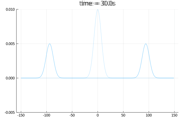
(a) Linear acoustic wave equation, eq. i

Overlapped initial and final time snapshots

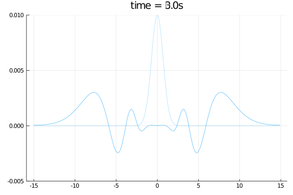
(b) Linearized water waves system, eq. ii

Figure i: Disintegration of Gaussian initial data, $\dzeta(\dt=0,\dx)=0.01\exp(-(0.1\,\dx)^{2})$ (left) and $\dzeta(\dt=0,\dx)=0.01\exp(-\dx^{2})$ (right), with zero initial velocities. $\dg=9.81\,{\rm m}.{\rm s}^{-2}$, $\dH=1\,{\rm m}$.

In dimension $d=2$, the solution is less explicit, but a formula can still be written—at least for sufficiently regular initial data—with the use of Green’s function (we could also use Fourier representation as in the next section):

$$\dzeta(\dt,\dbx)=\frac{1}{2\pi\dc_{0}}\int_{|\dby-\dbx|\leq\dc_{0}\dt}\frac{\partial_{\dt}\dzeta(0,\dby)}{\sqrt{(\dc_{0}\dt)^{2}-|\dby-\dbx|^{2}}}\operatorname{d\!}\dby+\frac{1}{2\pi\dc_{0}}\partial_{\dt}\int_{|\dby-\dbx|\leq\dc_{0}\dt}\frac{\dzeta(0,\dby)}{\sqrt{(\dc_{0}\dt)^{2}-|\dby-\dbx|^{2}}}\operatorname{d\!}\dby.$$

We can observe that the solution satisfies causality (but not Huygens’ principle): waves must be given enough time to propagate between two specified points. Again, $\dc_{0}$ is a good measure of the (scalar) velocity of waves according to eq. i. Less obvious is the fact that for sufficiently smooth and decaying initial data, the amplitude of the solution decays for large time as $(\dc_{0}\dt)^{-1/2}$. Figure ii represents the evolution of the surface deformation when taken initially as Gaussians (with zero initial velocities) according to eq. i and eq. ii, in dimension $d=2$.

Overlapped initial and final time snapshots

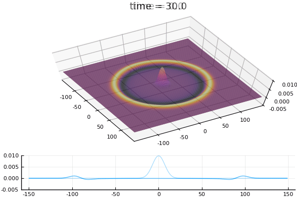
(a) Linear acoustic wave equation, eq. i

Overlapped initial and final time snapshots

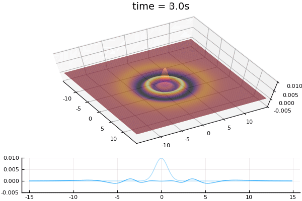
(b) Linearized water waves system, eq. ii

Figure ii: Disintegration of Gaussian initial data, with zero initial velocities.
$\dg=9.81\,{\rm m}.{\rm s}^{-2}$, $\dH=1\,{\rm m}$. The bottom plot represents the solution on $\{(\dx,\dy)\ :\ \dy=0\}$.

The linearized (Airy) water waves equations

The following equations describe the propagation of infinitesimally small waves without the long wave assumption of the previous section: it is the linearized system about the rest-state solution to the water waves equations, whose solutions shall be considered as “exact”, and which is introduced in Chapter A. Consider the linearized water waves equations as

$$\left\{\begin{array}[]{l}\partial_{\dt}\dzeta-\dmG_{0}\dpsi=0,\\[4.30554pt] \partial_{\dt}\dpsi+\dg\dzeta=0\end{array}\right.$$ (ii)

where $\dmG_{0}=|D|\tanh(\dH|D|)$ is the Fourier multiplier operator defined on sufficiently regular solutions by

$$\forall\dbxi\in\mathbb{R}^{d},\qquad\widehat{\dmG_{0}\dpsi}(\dbxi)=|\dbxi|\tanh(\dH|\dbxi|)\widehat{\dpsi}(\dbxi).$$

Here, $\dg$, $\dH$ and $\dzeta$ are as above and $\dpsi$ represents the trace of the velocity potential at the surface. Equation ii is a system of linear constant-coefficient equations of the form

$$\partial_{\dt}\begin{pmatrix}\dzeta\\ \dpsi\end{pmatrix}={\sf L}(D)\begin{pmatrix}\dzeta\\ \dpsi\end{pmatrix}$$

where ${\sf L}(D)$ is a matrix with Fourier multiplier coefficients.

Formally taking the limit $\dH\to 0$, we may replace $\tanh(\dH|\dbxi|)$ with $\dH|\dbxi|$ in $\dmG_{0}$, and then we recover the acoustic wave equation, eq. i. In fact using eq. ii instead of eq. i in the left side of Figure i and Figure ii yields a very similar outcome; such is not the case for the narrower initial data used for right sides.

Modal analysis

Plane waves of the form $(\dzeta,\dpsi)=(\dzeta_{0}e^{i(\dbxi\cdot\dbx-\domega\dt)},\dpsi_{0}e^{i(\dbxi\cdot\dbx-\domega\dt)})$ are solutions to eq. ii provided that $i\domega\dpsi_{0}=\dg\dzeta_{0}$ and the dispersion relation holds [245, 7]:

$$\domega(\dbxi)^{2}=\dg|\dbxi|\tanh(\dH|\dbxi|).$$

In other words, we can explicitly solve the equation in the Fourier space:

$$\begin{pmatrix}\widehat{\dzeta}(\dt,\dbxi)\\ \widehat{\dpsi}(\dt,\dbxi)\end{pmatrix}=\exp({\sf L}(\dbxi)\dt)\begin{pmatrix}\widehat{\dzeta}(0,\dbxi)\\ \widehat{\dpsi}(0,\dbxi)\end{pmatrix}=\begin{pmatrix}\cos(|\domega(\dbxi)|\dt)&\frac{|\domega(\dbxi)|}{\dg}\sin(|\domega(\dbxi)|\dt)\\ -\frac{\dg}{|\domega(\dbxi)|}\sin(|\domega(\dbxi)|\dt)&\cos(|\domega(\dbxi)|\dt)\end{pmatrix}\begin{pmatrix}\widehat{\dzeta}(0,\dbxi)\\ \widehat{\dpsi}(0,\dbxi)\end{pmatrix}.$$

For such plane wave solutions, $\domega$ is called the (angular) frequency, $\dbxi$ the (angular) wave vector (wavenumber if $d=1$), and $|\dbxi|$ the (angular) wavenumber. Phase velocities describe the velocity in a given direction of a plane wave with wave vector $\dbxi$, and satisfy

$${\dbc}_{p}\cdot\dbxi=\domega(\dbxi).$$

The group velocity represents the traveling velocity of a wave packet about wave vector $\dbxi$, and is given by

$$\dbc_{g}=\nabla_{\dbxi}(\domega(\dbxi)).$$

Misusing these definitions, we shall also refer to

$$\dc_{p}=\frac{|\domega(\dbxi)|}{|\dbxi|}=\sqrt{\dg\dH}\Big{(}\frac{\tanh(\dH|\dbxi|)}{\dH|\dbxi|}\Big{)}^{1/2}$$

as the phase velocity, and to

$$\dc_{g}=|\dbc_{g}|=\sqrt{\dg\dH}\left(\frac{1}{2}\Big{(}\frac{\tanh(\dH|\dbxi|)}{\dH|\dbxi|}\Big{)}^{1/2}+\frac{\operatorname{{sech}}^{2}(\dH|\dbxi|)}{2}\Big{(}\frac{\dH|\dbxi|}{\tanh(\dH|\dbxi|)}\Big{)}^{1/2}\right)$$

as the group velocity. They are represented in Figure iii. That the phase velocity is different (and greater) than the group velocity manifests the essential feature of the (linearized) water waves equations as being dispersive. Notice however that for small-normed wave vectors, $\dH|\dbxi|\ll 1$, both velocities converge to $\dc_{0}=\sqrt{\dg\dH}$, the velocity of (non-dispersive) infinitely long waves. In the opposite direction, for $\dH|\dbxi|\gg 1$, we have $\dc_{g}\sim\frac{1}{2}\dc_{p}\sim\frac{\sqrt{\dg}}{2|\dbxi|^{1/2}}$.

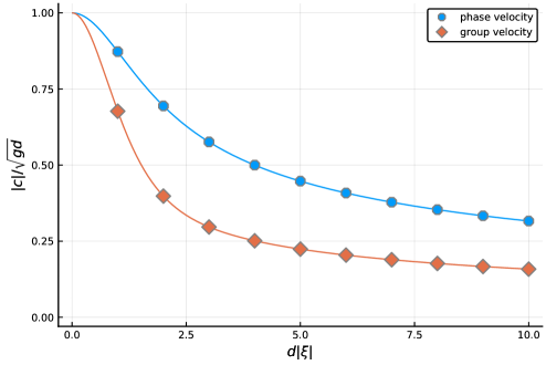
Figure iii: Phase and group velocities of the linearized water waves system.

Large-time behavior

We can infer the large-time behavior of the solution, at least in dimension $d=1$, through the stationary phase theorem on oscillatory integrals; see e.g.  [384]. Indeed, for any $\dc\in\mathbb{R}$, and initial data such that $(\widehat{\dzeta}(0,\cdot),|\domega|(\cdot)\widehat{\dpsi}(0,\cdot))\in L^{1}(\mathbb{R})^{2}$, we have from the above

$$\dzeta(\dt,\dc\dt)=\frac{1}{4\pi}\int_{\mathbb{R}}e^{i(\dc\dxi-\domega(\dxi))\dt}\left(\widehat{\dzeta}(0,\dxi)+i\frac{\domega(\dxi)}{\dg}\widehat{\dpsi}(0,\dxi)\right)+e^{i((\dc\dxi+\domega(\dxi))\dt}\left(\widehat{\dzeta}(0,\dxi)-i\frac{\domega(\dxi)}{\dg}\widehat{\dpsi}(0,\dxi)\right)\operatorname{d\!}\dxi$$

where we denote $\domega(\xi)=\operatorname{{sgn}}(\xi)(\dg|\xi|\tanh(\dH|\dxi|))^{1/2}$, and use a standard convention for the Fourier transform. We deduce that the following holds for sufficiently decaying and regular initial data.

1. For any $\dc\in(-\infty,-\sqrt{\dg\dH})\cup(\sqrt{\dg\dH},+\infty)$, one has for any $n\in\mathbb{N}$,

   $$|\dzeta|(\dt,\dc\dt)=\mathcal{O}(\dt^{-n}).$$

2. For any $\dc\in(-\sqrt{\dg\dH},\sqrt{\dg\dH})\setminus\{0\}$, one has

   $$|\dzeta|(\dt,\dc\dt)\sim_{t\to\infty}\frac{1}{4\pi}(2!)^{1/2}\Gamma(\tfrac{3}{2})|\dA(\dxi_{\dc})|\big{(}|\domega^{\prime\prime}(\dxi_{\dc})|\,\dt\big{)}^{-\frac{1}{2}}$$

   where $\dxi_{\dc}$ is defined by the relation $\dc=\domega^{\prime}(\dxi_{\dc})$ and $\dA(\dxi_{\dc})\stackrel{{\scriptstyle\rm def}}{{=}}\widehat{\dzeta}(0,\dxi_{\dc})+\operatorname{{sgn}}(\dc)i\frac{\domega(\dxi_{c})}{\dg}\widehat{\dpsi}(0,\dxi_{\dc})$; unless $\dA(\dxi_{\dc})=0$ in which case the decay is at least $\mathcal{O}(\dt^{-1})$.

3. If $\dc\in\{-\sqrt{\dg\dH},\sqrt{\dg\dH}\}$ , one has

   $$|\dzeta|(\dt,\dc\dt)\sim_{t\to\infty}\frac{1}{4\pi}(3!)^{\frac{1}{3}}\Gamma(\tfrac{4}{3})|\dA(0)|\big{(}\dH^{2}\sqrt{\dg\dH}\,\dt\big{)}^{-\frac{1}{3}}\approx\da\,((\dH^{2}/\dL^{2})\sqrt{\dg\dH}/\dL\dt)^{-\frac{1}{3}},$$

   with $\dA(0)\stackrel{{\scriptstyle\rm def}}{{=}}\lim_{\dxi\to 0}\dA(\dxi)$ (notice we require regularity only on $\dxi\widehat{\dpsi}(0,\dxi)$); unless $\dA(0)=0$, in which case the decay is at least $\mathcal{O}(\dt^{-\frac{2}{3}})$. The last approximation is meant in a loose sense, where we set $\dA(0)\approx\da\dL$. This allows to hint at the timescale for which dispersive mechanisms have a bearing on the behavior of the flow, which is large compared with the time period of long waves, $\dT\stackrel{{\scriptstyle\rm def}}{{=}}\dL/\sqrt{\dg\dH}$, when $\dH^{2}/\dL^{2}\ll 1$.

Above, $\Gamma$ is the Euler Gamma function: $\Gamma(s)\stackrel{{\scriptstyle\rm def}}{{=}}\int_{0}^{+\infty}\tau^{s-1}e^{-\tau}\operatorname{d\!}\tau$. A loose interpretation of the above is that for large time, the dominant part of the wave which will remain visible is the large wavelength component, traveling at velocity $|\dc|\approx\dc_{0}=\sqrt{\dg\dH}$.

The Saint-Venant system

Our first nonlinear model is the so-called shallow water, or Saint-Venant system system [364]:

$$\left\{\begin{array}[]{l}\partial_{\dt}\dzeta+\nabla\cdot(\ddh\dbu)=0,\\[4.30554pt] \partial_{\dt}\dbu+\dg\nabla\dzeta+(\dbu\cdot\nabla)\dbu={\bm{0}},\end{array}\right.$$ (iii)

where $\ddh\stackrel{{\scriptstyle\rm def}}{{=}}\dH+\dzeta$ represents the water depth, and $\dbu$ a horizontal velocity (it can be the layer-averaged horizontal velocity, velocity at a certain depth, or $\nabla\dpsi$). Pursuing the analogy of The linear acoustic wave equation, one can notice that the Saint-Venant system is equivalent to the isentropic, compressible Euler equation for ideal gases with the pressure law $\ddp(\drho)\propto\drho^{2}$ (identifying $\drho$ with $\ddh$).

System (iii) is hence a prototype of quasilinear hyperbolic systems. Hyperbolicity amounts to the non-cavitation assumption, that is restricting data to $\{(\dzeta,\dbu)\ :\ \dH+\dzeta>0\}$. Indeed, the system in dimension $d=2$ reads

$$\partial_{\dt}\begin{pmatrix}\dzeta\\ \du_{\dx}\\ \du_{\dy}\end{pmatrix}+\begin{pmatrix}\du_{\dx}&\ddh&0\\ \dg&\du_{\dx}&0\\ 0&0&\du_{\dx}\end{pmatrix}\partial_{\dx}\begin{pmatrix}\dzeta\\ \du_{\dx}\\ \du_{\dy}\end{pmatrix}+\begin{pmatrix}\du_{\dy}&0&\ddh\\ 0&\du_{\dy}&0\\ \dg&0&\du_{\dy}\end{pmatrix}\partial_{\dy}\begin{pmatrix}\dzeta\\ \du_{\dx}\\ \du_{\dy}\end{pmatrix}=\begin{pmatrix}0\\ 0\\ 0\end{pmatrix}$$

and the eigenvalues of the associated symbol (see e.g. [306]) are

$$\dbu\cdot\dbxi\quad\text{ and }\quad\dbu\cdot\dbxi\pm\sqrt{\dg\ddh}|\dbxi|\,.$$

Notice here again the “sound speed” of long surface gravity waves as being $\dc_{0}=\sqrt{\dg\dH}$.

In dimension $d=1$, as any quasilinear system of two scalar balance laws, eq. iii enjoys a basis of Riemann invariants. The Riemann invariants are explicit in this case: setting $\dr_{\pm}=\du\pm 2\sqrt{\dg\ddh}$, the system (iii) is equivalent to

$$\left\{\begin{array}[]{l}\partial_{\dt}\dr_{+}+\frac{3\dr_{+}+\dr_{-}}{4}\partial_{\dx}\dr_{+}=0,\\[4.30554pt] \partial_{\dt}\dr_{-}+\frac{3\dr_{-}+\dr_{+}}{4}\partial_{\dx}\dr_{-}=0.\end{array}\right.$$ (iv)

Notice that $\frac{3r_{+}+r_{-}}{4}=\du+\sqrt{\dg\ddh}$ and $\frac{3r_{-}+r_{+}}{4}=\du-\sqrt{\dg\ddh}$, consistently with the hyperbolicity discussion. The diagonal formulation, eq. iv, allows to construct simple waves, i.e. solutions of the form

$$(\dr_{+},\dr_{-})=\dbR(\dtheta(t,x))$$

where $\theta$ is a scalar function. For instance, any sufficiently regular solution to eq. iv with initial data satisfying $\du\left|{}_{{}_{\dt=0}}\right.=2\sqrt{\dg\ddh\left|{}_{{}_{\dt=0}}\right.}-2\sqrt{\dg\dH}$, the second equation yields $\dr_{-}\equiv-2\sqrt{\dg\dH}$ for all times, from which we deduce $\dr_{+}=2\sqrt{\dg\dH}+2\du$, where $\du(\dt,\dx)$ satisfies the inviscid Burgers (or Hopf) equation

$$\partial_{\dt}\du+\big{(}\sqrt{\dg\dH}+\tfrac{3}{2}\du\big{)}\partial_{\dx}\du=0.$$ (v)

Conversely, any solution to the above equation provides a particular solution to eq. iv by setting $(\dr_{-},\dr_{+})=(2\sqrt{\dg\dH}+2\du,-2\sqrt{\dg\dH})$, or equivalently a solution to eq. iii with $\dzeta=\dg^{-1}\big{(}\sqrt{\dg\dH}\du+\tfrac{1}{4}\du^{2}\big{)}$.

Equation v may be solved by the hodograph transform, or the characteristics method, and exhibits a new phenomenon with respect to the linear equations discussed in previous sections: finite-time singularity formation. Assume $\du$ is a Lipschitz solution to eq. v and define, for any $\dx_{0}\in\mathbb{R}$, $\dv_{\dx_{0}}(\dt)\stackrel{{\scriptstyle\rm def}}{{=}}\du(t,\dx_{\dx_{0}}(\dt))$ where $\dx_{\dx_{0}}(\dt)$ is defined by the initial condition $\dx_{\dx_{0}}(t)=\dx_{0}$ and the ordinary differential equation $\dx_{\dx_{0}}^{\prime}(\dt)=\sqrt{\dg\dH}+\tfrac{3}{2}\du(\dt,\dx_{\dx_{0}}(\dt))$. Chain rule and eq. v yields $\dv_{\dx_{0}}^{\prime}(\dt)=0$, and hence $\dv_{\dx_{0}}(\dt)=\du(0,\dx_{0})$ and finally $\dx_{\dx_{0}}(t)=\dx_{0}+(\sqrt{\dg\dH}+\tfrac{3}{2}\du(0,\dx_{0}))\dt$. In other words, the solution is constant along the characteristics defined by $\dx_{\dx_{0}}(\dt)$, for any $\dx_{0}\in\mathbb{R}$, and the characteristics are straight lines. This allows to define and describe solutions as long as two characteristics do not cross, i.e. as long as for any $\dt\in(0,\dT)$, there does not exists $\dx_{0}\neq\dx_{1}\in\mathbb{R}$ with

$$\dx_{0}+\big{(}\sqrt{\dg\dH}+\tfrac{3}{2}\du(0,\dx_{0})\big{)}\dt=\dx_{1}+\big{(}\sqrt{\dg\dH}+\tfrac{3}{2}\du(0,\dx_{1})\big{)}\dt\quad\Longleftrightarrow\quad\tfrac{\du(0,\dx_{1})-\du(0,\dx_{0})}{\dx_{1}-\dx_{0}}=-\tfrac{2}{3\dt}.$$

Hence we see that for any Lipschitz initial data $\du(\dt=0,\cdot)=\du_{0}\in W^{1,\infty}(\mathbb{R})$, the solution described above (which is unique) exists on the time domain $[0,\dT^{\star})$ where $\dT^{\star}=-\frac{2}{3}(\inf_{\mathbb{R}}\du_{0}^{\prime})^{-1}$ with the convention $\dT^{\star}=\infty$ if $\inf_{\mathbb{R}}\du_{0}^{\prime}\geq 0$. In the situation where $\inf_{\mathbb{R}}\du_{0}^{\prime}<0$ (in particular for any non-trivial $\du_{0}$ such that $\du_{0}\to 0$ as $|\dx|\to\infty$), there exists indeed a singularity formation as $t\to\dT^{\star}$: since the solution remains bounded but $\inf_{\mathbb{R}}\partial_{\dx}u(\dt,\cdot)\to-\infty$ as $\dt\nearrow\dT^{\star}$, we say that a shock, or a wavebreaking, occurs. We represent this situation in Figure iv.

Overlapped initial and final time snapshots

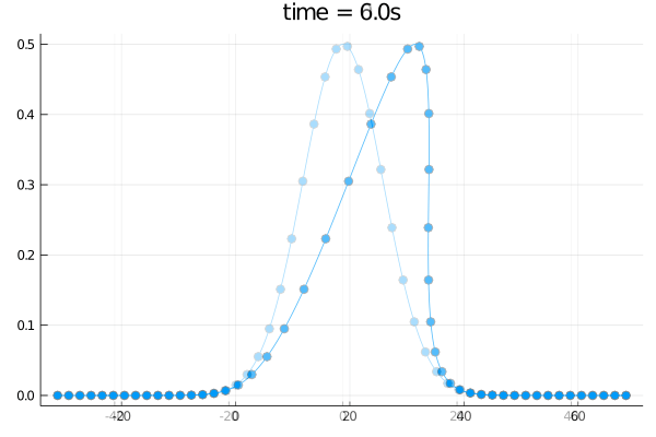
(a) Evolution in time

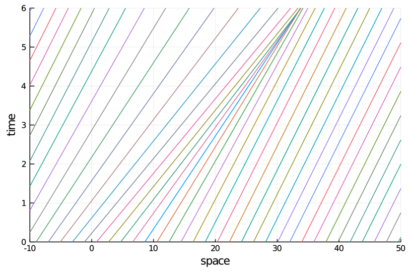
(b) Characteristics

Figure iv: Wavebreaking of a simple wave according to eq. v. The initial data for $\dzeta$ is the Gaussian $\dzeta(\dt=0,\dx)=0.5\exp(-(0.1\,\dx)^{2})$ and corresponding velocity. $\dg=9.81\,{\rm m}.{\rm s}^{-2}$, $\dH=1\,{\rm m}$.

Going back to the system case, eq. iv, each of the Riemann invariants, $\dr_{\pm}$, is constant along characteristics curves defined by

$$\dx_{\pm,\dx_{0}}(0)=\dx_{0},\quad\dx_{\pm,\dx_{0}}^{\prime}(\dt)=\frac{1}{4}(3\dr_{\pm}+\dr_{\mp})(\dt,\dx_{\pm,\dx_{0}}(\dt)).$$

However the characteristics curves are no longer straight lines in general. Still we can infer the behavior of solutions for instance if we assume that initial data $(\dzeta(t=0,\cdot),\du(t=0,\cdot))\stackrel{{\scriptstyle\rm def}}{{=}}(\dzeta_{0},\du_{0})$ have compact support, say in $(-\dL,\dL)$, and are are sufficiently small so that there exists $\dc\in(0,\dc_{0})$ with

$$\dr_{+,0}\stackrel{{\scriptstyle\rm def}}{{=}}\du_{0}+2\sqrt{\dH+\dzeta_{0}}\in(2\dc_{0}-\dc,2\dc_{0}+\dc)\quad\text{ and }\quad\dr_{-,0}\stackrel{{\scriptstyle\rm def}}{{=}}\du_{0}-2\sqrt{\dH+\dzeta_{0}}\in(-2\dc_{0}-\dc,-2\dc_{0}+\dc).$$

Because the Riemann invariants are constant along characteristics, we have, as long as the solution remains regular, $\frac{3\dr_{+}+\dr_{-}}{4}\in(\dc_{0}-\dc,\dc_{0}+\dc)$ and $\frac{3\dr_{-}+\dr_{+}}{4}\in(-\dc_{0}-\dc,-\dc_{0}+\dc)$, and as a consequence

$$\dr_{+}(\dt,\dx)\equiv 2\dc_{0}\text{ if $\dx\leq-\dL+(\dc_{0}-\dc)\dt$}\quad\text{ and }\quad\dr_{-}(\dt,\dx)\equiv-2\text{ if $\dx\geq\dL-(\dc_{0}-\dc)\dt$}.$$

If the initial data is sufficiently small in order to ensure that no shock formation occurs before $\dT_{\star}=\frac{\dL}{\dc-\dc_{0}}$, we can afterwards decompose the flow as the superposition of two simple waves described by Hopf equations, and in particular a shock inevitably occurs after sufficiently large time.

Boussinesq systems

In his celebrated manuscript [59], Boussinesq introduced the first models for the propagation of surface gravity waves taking into account both (first order) nonlinear and dispersive effects. While restricted in the original work to unidirectional waves, models with similar flavor were later on obtained for general waves. Eventually, one may obtain a full family of systems [290, 51], often called ($abcd$) Boussinesq systems, of the form

$$\left\{\begin{array}[]{l}\partial_{\dt}(\dzeta-b\dH^{2}\Delta\dzeta)+\nabla\cdot(\ddh\dbu+a\dH^{3}\nabla\nabla\cdot\dbu)=0,\\[4.30554pt] \partial_{\dt}(\dbu-d\dH^{2}\nabla\nabla\cdot\dbu)+\dg\nabla(\dzeta+c\dH^{2}\Delta\dzeta)+(\dbu\cdot\nabla)\dbu={\bm{0}},\end{array}\right.$$ (vii)

where $\mathfrak{p}=(a,b,c,d)\in\mathbb{R}^{4}$ is such that (when neglecting surface tension) $a+b+c+d=\tfrac{1}{3}$. In eq. vii the precise meaning of the velocity variable depends on the choice of the parameters. The freedom in the choice of $(a,b,c,d)\in\mathfrak{p}$ is at the same time a blessing—for instance one may tune parameters so as to enhance the accuracy of the dispersion relation—and a curse, since important properties of the system will typically depend on the choice of $(a,b,c,d)\in\mathfrak{p}$. In particular, the initial-value problem of a subfamily of eq. vii is strongly ill-posed, as can be seen from modal instabilities of the linearized equations about the rest state: the dispersion relation being

$$\domega(\dbxi)^{2}=\dg\dH|\dbxi|^{2}\frac{(1-a|\dH\dbxi|^{2})(1-c|\dH\dbxi|^{2})}{(1+b|\dH\dbxi|^{2})(1+d|\dH\dbxi|^{2})}\,$$

with right-hand side taking arbitrarily large negative values at large wavenumbers, $|\dbxi|$, for ill-chosen $(a,b,c,d)\in\mathfrak{p}$. Incidentally, this is also the case for the original “bad” Boussinesq equation, eq. vi. This is a useful reminder that consistency is not the only property to look for in a model.

In the other way, it is expected that for “good” choices of $(a,b,c,d)\in\mathfrak{p}$, dispersive properties of the Boussinesq systems prevent the wavebreaking scenario in the Saint-Venant model, eq. iii. As a matter of fact, for several families of parameters, $(a,b,c,d)\in\mathfrak{p}$, global-in-time existence and uniqueness of solutions have been proved (see [369, Remark 1.1]) and—to the author’s knowledge—the emergence of finite-time singularity has not been proved or numerically witnessed on any of the models, at least for solutions maintaining positive layer depth. In the situation of long waves and relatively large amplitude, the solution typically generates a zone of rapid oscillations (or modulations) often called dispersive shock wave, in place of the shock predicted by the Saint-Venant system. Properties of these dispersive shock waves will typically depend on the choice of $(a,b,c,d)\in\mathfrak{p}$, and is not expected to accurately describe the real-life phenomenon.

An important property of nonlinear and dispersive equations such as eq. vii is that they allow the existence of traveling waves, that is solutions that maintain their shape while propagating at a constant velocity, including solitary waves which in addition bear finite energy. Once again the reader will find in [132] the fascinating and tumultuous story of the discovery and progressive acceptance of these waves. Existence and properties of traveling waves again typically depend on the choice of $(a,b,c,d)\in\mathfrak{p}$. We however expect that they exist at least for small supercritical velocities, $0<\dc-\dc_{0}\ll 1$, and grow in amplitude with the velocity parameter; see e.g. [140]. We show examples in Figure v.

Overlapped initial and final time snapshots

(a) Disintegration of Gaussian initial data

Overlapped initial and final time snapshots

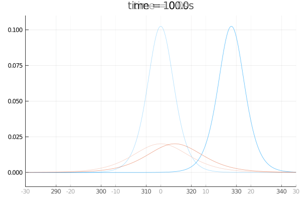
(b) Traveling waves

Figure v: Left: Disintegration of the Gaussian $\dzeta(\dt=0,\dx)=0.25\exp(-0.1\dx^{2})$, with zero initial velocity. Right: Solitary wave solutions with velocities $\dc=1.05\dc_{0}$ and $\dc=1.01\dc_{0}$.
Both according to system (vii) with $-a=b=d=\tfrac{1}{3}$, $c=0$, $\dg=9.81\,{\rm m}.{\rm s}^{-2}$, $\dH=1\,{\rm m}$.

It would be impossible to review all known results on Boussinesq systems and closely related (symmetric, Abbott, etc.) variants. Let me lazily refer to [149, 264, 369]—in addition to previous references—and references therein, and conclude with a last warning. The Boussinesq systems typically lose important properties of the original water waves equations and in particular its Hamiltonian structure. Hence unless the parameters $(a,b,c,d)\in\mathfrak{p}$ are well-chosen,we do not expect energy conservation, or Galilean invariance, etc.

The Korteweg–de Vries and Whitham equations

It was mentioned in the previous section that Boussinesq’s original motivation was the study of unidirectional waves, and in particular solitary waves. Using such assumption one may derive (as did Boussinesq) simplified scalar equations, of which the most famous is the Korteweg–de Vries equation [61, 257] for right-going waves in dimension $d=1$:

$$\partial_{\dt}\dzeta+\sqrt{\dg\dH}\partial_{\dx}(\dzeta+\tfrac{3}{4\dH}\dzeta^{2}+\tfrac{1}{6}\dH^{2}\partial_{\dx}^{2}\dzeta)=0\,.$$ (viii)

One of the many reasons for the importance of the Korteweg–de Vries equation is the family of explicit solitary wave solutions

$$\dzeta(\dt,\dx)=\dzeta_{\dc}(\dx-\dc t),\qquad\dzeta_{\dc}(\dx)\stackrel{{\scriptstyle\rm def}}{{=}}2\dH(\tfrac{\dc}{\dc_{0}}-1)\operatorname{{sech}}^{2}\big{(}\sqrt{\tfrac{3}{2\dH^{2}}(\tfrac{\dc}{\dc_{0}}-1)}\,\dx\big{)}$$

where the velocity variable, $\dc$, may take any value $\dc>\dc_{0}=\sqrt{\dg\dH}$.

The existence of traveling waves with arbitrarily large amplitude and arbitrarily large velocity may found undesirable as nonphysical [387]. Such is the case also for the global-in-time well-posedness properties, preventing the aforedescribed wavebreaking scenario. With this in mind, Whitham [406] introduced the following equation which is now called Whitham equation:

$$\partial_{\dt}\dzeta+\sqrt{\dg\dH}\partial_{\dx}\Big{(}\sqrt{\tfrac{\tanh(\dH|D|)}{\dH|D|}}\dzeta+\tfrac{3}{4\dH}\dzeta^{2}\Big{)}=0\,.$$ (x)

arguing that the fact that its linear dispersion relation reproduces exactly one branch of the dispersion relation of eq. ii would authorize wavebreaking and peaked traveling waves of extreme height. This prediction turned out to be valid, as recently shown in [216, 172, 396, 368]. A numerical comparison of solitary wave solutions to the Korteweg–de Vries and Whitam equations is shown in Figure vi.

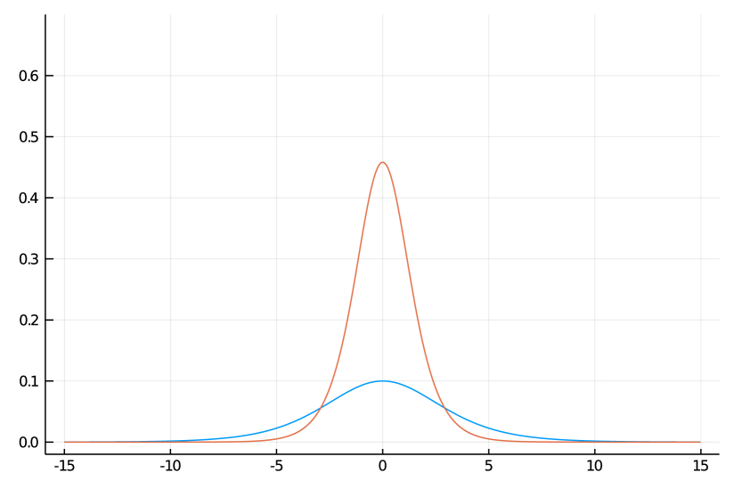
(a) KdV equation, eq. viii

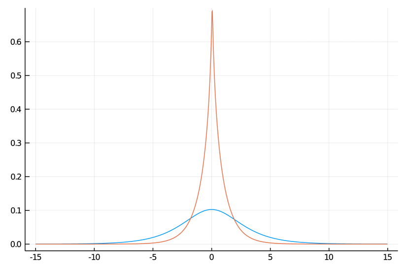
(b) Whitham equation, eq. x

Figure vi: Solitary waves of unidirectional models with velocity $\dc=1.05\dc_{0}$ (blue, smaller) and $\dc=1.2290408\dc_{0}$ (red, larger). $\dg=9.81\,{\rm m}.{\rm s}^{-2}$, $\dH=1\,{\rm m}$, $\dc_{0}=\sqrt{\dg\dH}$.

Chapitre A The “master” equations

Le problème de l’établissement […] des équations différentielles du mouvement, et ensuite de leur intégration approchée, aura encore sa difficulté souvent grande. Mais il ne présentera plus, envisagé ainsi, cette désespérante énigme contre laquelle des esprits distingués se sont heurtés en vain.

— Adhémar Barré de Saint-Venant, Comptes rendus des séances de l’Académie des sciences, séance du 18 mars 1872

Foreword

In this chapter, we introduce and provide a preliminary study of the systems of equations from which asymptotic models are derived in subsequent chapters. The presentation, as well as most of the notations, are borrowed from Lannes’ book [263]. However concision has been pursued and I cannot encourage enough a thorough reading of the book for a detailed account.

We first write down the most general system of equations which is considered in this work, that is Euler equations for a layer of (non-necessarily homogeneous) incompressible ideal fluid, coupled with boundary conditions accounting for the impermeable bottom and the free surface. The only external force acting on the system will be the gravity force, assumed constant and vertical. We refer to the system we obtain as the full Euler system. Then we focus on particular settings.

The homogeneous and irrotational framework is particularly rewarding, as it allows to rewrite the whole system as two evolution equations for unknown functions of time and horizontal space variables only. This system is referred to as the water waves equations.

Prominently important in the water waves equations is the Dirichlet-to-Neumann operator, which is defined after solving a Laplace problem on the fluid domain with Dirichlet and Neumann boundary conditions. Its study, and in particular the asymptotic expansions which allow to derive asymptotic models, are briefly reviewed.

Meanwhile we make a small step outside the world of homogeneous and potential flows to consider interfacial waves between two layers of homogeneous fluids with irrotational velocities. Additional Dirichlet/Neumann operators appearing in this framework are tackled.

Chapitre B Hydrostatic models

“Begin at the beginning," the King said gravely, “and go on till you come to the end: then stop."

— Lewis Carroll, Alice in Wonderland

Figure B: Models in Chapter B (in green) and some filiations.

Foreword

We start our journey towards asymptotic models with ones among the oldest and simplest-looking. The so-called hydrostatic models can be formally derived from the “master” full Euler equations by using the hydrostatic assumption, that is approximating the pressure terms using an explicit formula stemming from neglecting the velocity advection terms in the horizontal momentum conservation equation, specifically

$$-\partial_{\dz}\dP=\drho\dg,$$

which we can integrate using the known pressure at the free surface. Additionally, one often adds the assumption of columnar motion, stating that the horizontal velocity (approximately) does not depend on the vertical variable. When both assumptions are made, then we quickly obtain models with the rewarding properties that the vertical space variable has disappeared from the equations and only (first order) differential operators are involved.

Yet we shall not assume a priori—but indirectly prove—the hydrostatic assumption nor the columnar motion and will rather justify models asymptotically—with quantitative error estimates—in the shallow water regime, as $\mu\ll 1$; and using the irrotationality assumption in lieu of columnar motion.

Our first model is derived from the water waves system, that is assuming that the density is homogeneous and the flow potential (as this allows to discard the vertical variable except in the Dirichlet-to-Neumann operator). We then obtain the well-known and much-studied Saint-Venant system, already introduced in The Saint-Venant system. Its derivation and rigorous justification, together with a very short description of some of its properties, is the subject of a first section.

Then we move to the bilayer framework, with two layers of homogeneous potential flows. The situation is slightly messier as models differ whether we use the free-surface framework or the rigid-lid framework, and in the latter one often uses the so-called Boussinesq approximation. It turns out the rigid-lid assumption and Boussinesq approximation both follow from the same assumption of weak density contrast.

Finally we quickly extend the analysis to $N\geq 2$ layers as above. While this multilayer framework may appear artificial, it is expected to approximate (as $N\gg 1$) the setting of continuously stratified flows, in view of withdrawing the assumptions of homogeneous density and potential flows while keeping the hydrostatic approximation in the shallow water regime.

Hydrostatic equations for continuously stratified flows are also discussed. It turns out very little is known on these equations, despite the fact that they are at the core of the primitive equations which are widely used in studies and numerical simulations of geophysical flows. This offers stimulating mathematical challenges.

Chapitre C Weakly dispersive models

parce que, [les Anciens] s’étant élevés jusqu’à un certain degré où ils nous ont portés, le moindre effort nous fait monter plus haut, et avec moins de peine et moins de gloire nous nous trouvons au-dessus d’eux. C’est de là que nous pouvons découvrir des choses qu’il leur était impossible d’apercevoir.

— Blaise Pascal, traité du vide

Figure C: Models in Chapter C (in green) and some filiations.

Foreword

This chapter is devoted to the derivation and analysis of weakly dispersive models. These models refine the hydrostatic equations studied in Chapter B (in fact, more precisely, the Saint-Venant equations since here we restrict the analysis to the water waves framework; see Chapter E for an extension to the bilayer framework) by introducing dispersive effects at first order. More refined models are presented in Chapter D.

The first section of this chapter has been meant as a showcase for a thorough study of water waves models. Here we introduce and analyze the so-called (Serre–)Green–Naghdi model. Firstly the model is quickly derived as an asymptotic model from the expansion of the Dirichlet-to-Neumann operator obtained in Chapter A. Yet the result which follows (namely the consistency of the model) is far from being sufficient to validate the Green–Naghdi equations as a good model for water waves. Firstly, its rigorous justification must be completed by well-posedness, stability and convergence results. They follow from careful energy estimates in suitable functional spaces. In a looser way, we also expect “good” models to retain important properties of the master equations (here the water waves system). Here we focus mostly on the variational structure of the equations: we observe that the Green–Naghdi equations not only preserve Zakharov’s canonical Hamiltonian structure of the water waves system, but it also enjoys a deeper Lagrangian formalism which embeds the system inside a natural family of conservation laws, which can be interpreted as equations for compressible fluids with inertia effects. Hence the structure of the equations becomes richer as we simplify the equations from the water waves system to the Green–Naghdi equations (and then from the Green–Naghdi equations to the Saint-Venant system). This explains in my opinion why the Green–Naghdi equations, among many other loosely equivalent models, has attracted so much attention from diverse communities. We review some basic properties of the Green–Naghdi equations: preserved quantities, modal analysis and dispersion relation, solitary wave solutions. Finally, some open questions are discussed.

Of course I do not claim that the Green–Naghdi model is perfect! One of its main drawback is certainly that numerically approximating the equations turns out to be quite costly. In a second section we explore some equations which have been proposed by Favrie and Gavrilyuk [180] to circumvent this issue. The equations are constructed using the aforementioned Lagrangian formalism, using a strategy akin to relaxation limits. Hence the system contains additional unknowns as well as a (large) parameter which is expected to measure the precision of solutions to the augmented equations with respect to solutions to the original Green–Naghdi equations, at least when initial data are well-prepared. The rigorous study of this singular limit is based on [156]. Again, the section is concluded by perspectives and open questions.

In a third section we introduce a fully dispersive analogue of the Green–Naghdi system, which we name Whitham–Green–Naghdi. When linearized about trivial equilibrium solutions, fully dispersive models coincide with the corresponding (Airy) linearized water waves equations, as introduced in The linearized (Airy) water waves equations. Interest in such fully dispersive models in the context of long water waves started with the work of Whitham, which proposed eq. x and eq. ix as suitable modifications of the standard Korteweg-de Vries equation, eq. viii, in view of reproducing at least qualitatively important features of water waves such as wavebreaking and peaked traveling waves. Much more recently, the interest was renewed as Whitham’s predictions were proved to be valid [216, 172, 396, 368]. Yet the question of validating fully dispersive models as asymptotic models with improved accuracy with respect to their standard counterparts was mostly left aside. The precision of the Whitham–Green–Naghdi model (respectively Whitham–Boussinesq) introduced in this section significantly improves the precision of the Green–Naghdi (respectively Boussinesq) model for weak nonlinearities and mild bottom variations with the important price to pay that nonlocal operators (Fourier multipliers) are involved. These models also allow to rigorously justify the Whitham equations and observe a similar improvement with respect to the Korteweg–de Vries equation [176].

Chapitre D Higher order models

Jésus a dit : « Que celui qui cherche ne cesse pas de chercher, jusqu’à ce qu’il trouve. Et quand il aura trouvé, il sera troublé ; quand il sera troublé, il sera émerveillé, et il régnera sur le Tout. »

— Thomas l’apôtre, évangile selon Thomas

Figure D: Models in Chapter D (in green) and some filiations.

Foreword

In this chapter we introduce and discuss higher order models for the water waves system, building upon the Saint-Venant system (Chapter B) and the Green–Naghdi system (Chapter C). These are hierarchies of models, that is families of system depending on a parameter—always denoted $N$—which we call the rank of the model, of which the Saint-Venant and/or the Green–Naghdi system are typically the first rank elements. The Saint-Venant (resp. Green–Naghdi) system has been rigorously justified as a shallow water model for the water waves system, in—roughly speaking—the following way: the size of the difference between solutions to the dimensionless water waves system and the corresponding solutions to the model equations grows proportionally to the size of the initial data with a prefactor bounded as $C\,\mu\,t$ (resp. $C\,\mu^{2}\,t$) over a relevant time interval (being of size inversely proportional to the size of the initial data), where $\mu$ is the shallow water parameter, and $C$ depends on an upper bound on the size of the admissible initial data (together with a lower bound on the minimal depth of the layer, an upper bound on admissible values for $\mu$, and the norms measuring the size of the data). In good cases we expect that a similar result holds for all elements in a hierarchy of models, with different prefactors $C_{N}\,\mu^{\alpha_{N}}\,t$. There are typically two situations:

1. the order as a shallow water model increases with $N$, that is $\alpha_{N}\to\infty$ as $N\to\infty$;

2. the accuracy of the model improves with $N$, that is $C_{N}\to 0$ as $N\to\infty$.

In the latter but not in the former we can hope that the hierarchy provides a robust tool for the approximation of any (sufficiently regular) solution to the water waves system, and can be useful for instance to devise strategies for their numerical integration.

This chapter is decomposed into three sections, corresponding to three different strategies, each producing a variety of families of higher order models.

In the first section, we use an expansion due to Boussinesq [60] and Rayleigh [357] (see [139, §4.1] for discussion and other relevant references) of the velocity potential—as a solution to the Laplace problem—as a series involving powers of the shallow water parameter, $\mu$. We are hence typically in the framework of the first aforementioned situation, and this section emphasizes its possible shortcomings. Among the different models which can be naturally constructed by this way—which we call Friedrichs-type systems in acknowledgment to his Appendix to [386]—we introduce explicitly two families of models: the high order shallow water models and the extended Green–Naghdi models. These models involve differential operators of increasing order as the rank of the model grows, which yields several complications. Firstly, half of these models suffer from very serious high frequency instabilities which prevent any hope as for the well-posedness of the Cauchy problem. But even in good cases, it is expected that for fixed initial data the solutions to the systems—if they exist—do not converge towards the corresponding solution to the water waves system, as $N\to\infty$. This can be seen in particular when studying the dispersion relation of the models, which converge towards the dispersion relation of the water waves system only for wavenumbers in a finite-size neighborhood of the origin.

In the second section we set up a Galerkin dimension reduction strategy to a reformulation of the Laplace problem, to devise the approximate formula for the velocity potential—or, more precisely, the horizontal velocity. As a second step, the usual procedure consists in using this approximate formula in the Hamiltonian functional of the water waves system, and express the model as the canonical Hamiltonian equations associated with the approximate Hamiltonian. This procedure produces a different model for any (reasonable) choice of subspace of real-valued functions of the fluid domain used in the Galerkin method. Natural examples of such spaces in the shallow water framework are functions of the form

$$\Phi(t,{\bm{x}},z)=\sum_{i=1}^{N}\phi_{i}(t,{\bm{x}})\,\Psi_{i}({\bm{x}},z) \star$$ ()

where $\phi_{i}(t,{\bm{x}})$ are variable unknowns of the resulting model, which is characterized by the choice of the vertical distribution, $\{\Psi_{i}\}_{i\in\{1,\dots,N\}}$. We explore the outcome of vertical distribution defined, following the finite element method, as piecewise polynomials in the vertical variable, $z$. We particularly emphasize two families of models (respectively playing with the degrees of the polynomials and the number of elements in the vertical discretization): the augmented Green–Naghdi models and the “multilayer” Green–Naghdi models. In each case, the system consists in two evolution equations coupled with a system of differential equations of order two mimicking the Laplace problem. The first family is a higher order shallow water hierarchy comparable to the models of the preceding section, yet instead of involving high order differential operators, the size of the system of differential equations grows with the rank, $N$. The second family has different properties, akin to the second situation described above. The term “multilayer” stems from the fact that the models can be interpreted as resulting from the vertical discretization of the fluid layer in $N$ prescribed—typically proportional—sublayers.

In the third section we describe the strategy referred in [256, 255] as “variational” (see [349] for an overview of related earlier and subsequent works). Of course the preceding strategy was also variational in nature, and we argue that the two strategies in fact differ only by the choice of the variational formulation of the Laplace problem. Yet in the latter, we plug directly the decomposition into Luke’s Lagrangian action for the water waves system, and let Hamilton’s principle do all the work in one single step. The outcome is surprising at first, as we obtain an overdetermined/underdetermined composite system of $N$ evolution equations for the surface deformation, $\zeta$, and only one evolution equation for $(\phi_{1},\ldots,\phi_{N})$. Yet the systems can in fact be written—as in the above hierarchies—under a canonical Hamiltonian formulation of two evolution equations coupled with a system of differential equations of order two. Again each choice of the vertical distribution, $\{\Psi_{i}\}_{i\in\{1,\dots,N\}}$, yields a different model. We only quickly mention the “multilayer” systems and instead focus on the shallow water system named the Isobe–Kakinuma models in reference to [228, 234]. Indeed the latter benefit from a rigorous justification theory, thanks to the work of Iguchi and collaborators, culminating with [223].

Chapitre E Non-hydrostatic models for interfacial waves

Toujours vouloir tout essayer, et recommencer

— Michel Berger, Le paradis blanc

Figure E: Models in Chapter E (in green) and some filiations.

Foreword

In Chapter A the equations extending the water waves system to the framework of interfacial waves between two layers of incompressible, homogeneous, inviscid and immiscible fluids with potential flows are introduced. The physical motivation for studying such systems is the reported (and ubiquitous) existence of coherent waves traveling at the sharp interface between, say, fresh and warm water above denser salted cold water. One can refer to e.g.  [230, 210] for a small peek at the vast literature on the subject. The main features of these waves is that they have tremendously large amplitudes—sometimes of the order of magnitude of the layer itself—, very long wave length, and travel over very long distances. Hence the assumptions of the shallow water regime, and in particular the fact that we do not impose any smallness assumption on the amplitude of the wave, is perfectly suited to the study of such waves. It is therefore very tempting to introduce asymptotic models for interfacial waves which are analogous to the asymptotic models for the water waves system. This is done in the hydrostatic framework in Chapter B and non-hydrostatic models are the subject of this chapter.

In addition to the physical motivation, there are interesting new features and challenges when studying interfacial waves. First and foremost, three additional dimensionless parameters come into view, namely

$$\alpha=\frac{\da_{\rm top}}{\da_{\rm int}}\quad;\quad\delta=\frac{\dH_{1}}{\dH_{2}}\quad;\quad\gamma=\frac{\drho_{1}}{\drho_{2}}$$

respectively the amplitude ratio of the free surface and interface, the depth ratio between the two layers, and the density ratio. Hence there are plethora of interesting limits to consider. We will focus here on the framework which is the most similar to the one-layer case and in particular we will assume that the two layers are of comparable depth, both small with respect to the typical horizontal wavelength of the flow. The relation between the limit of small density contrast, $\gamma\nearrow 1$ and the rigid-lid hypothesis, is discussed in details in the hydrostatic framework in Chapter B. Somewhat inconsistently, we will restrict henceforth to the rigid-lid situation without assuming the Boussinesq approximation, yet allowing $\gamma$ to approach unity. To summarize, our results hold for parameters in the following set.

Definition (Shallow water/Shallow water asymptotic regime).

Given $\mu^{\star},\delta_{\star},\delta^{\star}>0$, we let

$$\mathfrak{p}_{{\tfrac{\cramped[\scriptscriptstyle]{\rm SW}}{\cramped[\scriptscriptstyle]{\rm SW}}}}=\big{\{}(\mu,\varepsilon,\beta,\delta,\gamma)\ :\ \mu\in(0,\mu^{\star}],\ \varepsilon\in[0,1],\ \beta\in[0,1],\ \delta\in[\delta_{\star},\delta^{\star}],\gamma\in[0,1)\big{\}}.$$

One of the main striking difference between the water waves system and the corresponding interfacial waves system is the emergence of Kelvin–Helmholtz instabilities in the latter. Recall that the provided modal analysis shows that large wavenumber modes are unstable, and that the exponential growth rate takes arbitrarily large values as the wavenumber goes to infinity. This explains why the initial-value problem associated with the nonlinear system is strongly ill-posed outside of the analytic framework. This appears to contradict the fact that, as we said, large interfacial waves do exist and appear remarkably stable! An answer to this paradox has been given by Lannes in [262], by introducing interfacial tension effects: it is shown that well-posedness is restored, and more importantly the time of existence of solutions grows as $\mu\searrow 0$, consistently with the fact that the hydrostatic equations for interfacial waves are well-posed. It should be emphasized however that interfacial tension is not physical at the interface between two miscible fluids such as fresh and salted water; here it plays the role of a regularizing operator acting mostly on the high (spatial) frequency component of the flow. The real physical explanation is that mixing occurs, yet on a very thin transition layer: the pycnocline. In the absence—to my knowledge—of a simple expression revealing the effective influence of such mixing in the equations, we shall discard any effect when deriving asymptotic models.

It should be emphasized however that the models studied in this manuscript behave very differently regarding Kelvin–Helmholtz instabilities. Indeed, as the derivation focuses on the low frequency (large wavelength) component of the flow, the high frequency behavior can be very dissimilar between the different models, and hence with respect to the original interfacial waves system. A key revelation of the forthcoming study is the following.

• The Miyata–Choi–Camassa model, which is analogous to the Green–Naghdi system (see Chapter C), overestimates Kelvin–Helmholtz instabilities.

• This unfortunate behavior can be corrected through artificial—but harmless for the precision (in the sense of consistency) of the asymptotic model—modifications, which naturally yields fully dispersive systems named Whitham–Choi–Camassa; or regularized systems.

• The Kakinuma model, which extends the Isobe–Kakinuma model (see Chapter D) to the bilayer framework, inherently tames Kelvin–Helmholtz instabilities.

The latter model can be expected to be useful for understanding the propagation of long interfacial waves, focusing on the large-scale dynamics of the flow, and discarding small-scale effects as irrelevant. Once again, this should not blurry the fact that mixing do occur, and may in some circumstances play an important role on the large-scale dynamics. Models with the aim of tracking these effects—at least at first order—should use the continuously stratified Euler equations as a starting point. Yet as mentioned in Chapter B, very little is known for this system in the shallow water regime. An important reference—in my opinion—dealing with long weakly dispersive internal (and not interfacial) waves is [137]. The Perspectives section in that reference supports and complements the present discussion.

Appendix

- [1] H. D. I. Abarbanel, D. D. Holm, J. E. Marsden, and T. S. Ratiu. Nonlinear stability analysis of stratified fluid equilibria. Philos. Trans. Roy. Soc. London Ser. A, 318(1543):349–409, 1986.
- [2] M. Abbott, H. Petersen, and O. Skovgaard. On the numerical modelling of short waves in shallow water. J. Hydr. Res., 16(3):173–204, 1978.
- [3] M. B. Abbott, A. D. McCowan, and I. R. Warren. Accuracy of short-wave numerical models. J. Hydr. Eng. ASCE, 110(10):1287–1301, 1984.
- [4] M. Abramowitz and I. A. Stegun. Handbook of mathematical functions with formulas, graphs, and mathematical tables, volume 55 of National Bureau of Standards Applied Mathematics Series. U.S. Government Printing Office, Washington, D.C., 1964.
- [5] P. Aceves-Sánchez, A. A. Minzoni, and P. Panayotaros. Numerical study of a nonlocal model for water-waves with variable depth. Wave Motion, 50(1):80–93, 2013.
- [6] A. Ai, M. Ifrim, and D. Tataru. Two dimensional gravity waves at low regularity II: Global solutions. arXiv preprint:2009.11513.
- [7] G. B. Airy. Tides and waves. Encycl. Metropolitana, 5:291–396, 1845.
- [8] N. Aïssiouene, M.-O. Bristeau, E. Godlewski, A. Mangeney, C. Parés Madroñal, and J. Sainte-Marie. A two-dimensional method for a family of dispersive shallow water models. SMAI J. Comput. Math., 6:187–226, 2020.
- [9] T. Alazard. A minicourse on the low Mach number limit. Discrete Contin. Dyn. Syst. Ser. S, 1(3):365–404, 2008.
- [10] T. Alazard, N. Burq, and C. Zuily. The water-wave equations: from Zakharov to Euler. In Studies in phase space analysis with applications to PDEs, volume 84 of Progr. Nonlinear Differential Equations Appl., pages 1–20. Birkhäuser/Springer, New York, 2013.
- [11] T. Alazard, N. Burq, and C. Zuily. On the Cauchy problem for gravity water waves. Invent. Math., 198(1):71–163, 2014.
- [12] T. Alazard, N. Burq, and C. Zuily. Cauchy theory for the gravity water waves system with non-localized initial data. Ann. Inst. H. Poincaré Anal. Non Linéaire, 33(2):337–395, 2016.
- [13] S. Alinhac and P. Gérard. Opérateurs pseudo-différentiels et théorème de Nash-Moser. Savoirs Actuels. InterEditions et Editions du CNRS, Paris, 1991.
- [14] B. Alvarez-Samaniego and D. Lannes. Large time existence for 3D water-waves and asymptotics. Invent. Math., 171(3):485–541, 2008.
- [15] B. Alvarez-Samaniego and D. Lannes. A Nash-Moser theorem for singular evolution equations. Application to the Serre and Green-Naghdi equations. Indiana Univ. Math. J., 57(1):97–131, 2008.
- [16] D. M. Ambrose. Well-posedness of vortex sheets with surface tension. SIAM J. Math. Anal., 35(1):211–244 (electronic), 2003.
- [17] D. M. Ambrose, J. L. Bona, and D. P. Nicholls. On ill-posedness of truncated series models for water waves. Proc. R. Soc. Lond. Ser. A Math. Phys. Eng. Sci., 470(2166):20130849, 16, 2014.
- [18] D. M. Ambrose, R. Camassa, J. L. Marzuola, R. M. McLaughlin, Q. Robinson, and J. Wilkening. Numerical Algorithms for Water Waves with Background Flow over Obstacles and Topography. arXiv preprint:2108.01786.
- [19] D. M. Ambrose and N. Masmoudi. Well-posedness of 3D vortex sheets with surface tension. Commun. Math. Sci., 5(2):391–430, 2007.
- [20] D. Ambrosi. Hamiltonian formulation for surface waves in a layered fluid. Wave Motion, 31(1):71–76, 2000.
- [21] C. J. Amick. Regularity and uniqueness of solutions to the Boussinesq system of equations. J. Differential Equations, 54(2):231–247, 1984.
- [22] C. J. Amick, L. E. Fraenkel, and J. F. Toland. On the Stokes conjecture for the wave of extreme form. Acta Math., 148:193–214, 1982.
- [23] C. J. Amick and J. F. Toland. On solitary water-waves of finite amplitude. Arch. Rational Mech. Anal., 76(1):9–95, 1981.
- [24] D. Andrade and A. Nachbin. A three-dimensional Dirichlet-to-Neumann operator for water waves over topography. J. Fluid Mech., 845:321–345, 2018.
- [25] D. C. Antonopoulos, V. A. Dougalis, and D. E. Mitsotakis. On the well-posedness of the Galerkin semidiscretization of the periodic initial-value problem of the Serre equations. arXiv preprint:2107.04403.
- [26] L. Armi. The hydraulics of two flowing layers with different densities. J. Fluid Mech., 163:27–58, 1986.
- [27] K. Asano. On the incompressible limit of the compressible Euler equation. Japan J. Appl. Math., 4(3):455–488, 1987.
- [28] G. A. Athanassoulis and K. A. Belibassakis. A consistent coupled-mode theory for the propagation of small-amplitude water waves over variable bathymetry regions. Journal of Fluid Mechanics, 389:275–301, 1999.
- [29] G. A. Athanassoulis and C. E. Papoutsellis. Exact semi-separation of variables in waveguides with non-planar boundaries. Proc. A., 473(2201):20170017, 18, 2017.
- [30] E. Audusse, M.-O. Bristeau, M. Pelanti, and J. Sainte-Marie. Approximation of the hydrostatic Navier-Stokes system for density stratified flows by a multilayer model: kinetic interpretation and numerical solution. J. Comput. Phys., 230(9):3453–3478, 2011.
- [31] E. Audusse, M.-O. Bristeau, B. Perthame, and J. Sainte-Marie. A multilayer Saint-Venant system with mass exchanges for shallow water flows. Derivation and numerical validation. ESAIM Math. Model. Numer. Anal., 45(1):169–200, 2011.
- [32] K. I. Babenko. Some remarks on the theory of surface waves of finite amplitude. Dokl. Akad. Nauk SSSR, 294(5):1033–1037, 1987.
- [33] H. Bae and R. Granero-Belinchón. Singularity formation for the Serre-Green-Naghdi equations and applications to abcd-Boussinesq systems. arXiv preprint:2001.11937.
- [34] H. Bahouri, J.-Y. Chemin, and R. Danchin. Fourier analysis and nonlinear partial differential equations, volume 343. Springer, 2011.
- [35] P. G. Baines. A general method for determining upstream effects in stratified flow of finite depth over long two-dimensional obstacles. J. Fluid Mech., 188:1–22, 1988.
- [36] D. Bambusi. Hamiltonian studies on counter-propagating water waves. Water Waves, pages 1–35, 2020.
- [37] C. Bardos and N. Besse. The Cauchy problem for the Vlasov-Dirac-Benney equation and related issues in fluid mechanics and semi-classical limits. Kinet. Relat. Models, 6(4):893–917, 2013.
- [38] C. Bardos and N. Besse. Hamiltonian structure, fluid representation and stability for the Vlasov-Dirac-Benney equation. In Hamiltonian partial differential equations and applications, volume 75 of Fields Inst. Commun., pages 1–30. Fields Inst. Res. Math. Sci., Toronto, ON, 2015.
- [39] R. Barros and W. Choi. On the hyperbolicity of two-layer flows. In Frontiers of applied and computational mathematics, pages 95–103. World Sci. Publ., Hackensack, NJ, 2008.
- [40] E. Barthélemy. Nonlinear shallow water theories for coastal waves. Surveys in Geophysics, 25(3-4):315–337, 2004.
- [41] C. Bassi, L. Bonaventura, S. Busto, and M. Dumbser. A hyperbolic reformulation of the Serre-Green-Naghdi model for general bottom topographies. Comput. & Fluids, 212:104716, 21, 2020.
- [42] S. Bazdenkov, N. Morozov, and O. Pogutse. Dispersive effects in two-dimensional hydrodynamics. In Soviet Physics Doklady, volume 32, page 262, 1987. In Russian.
- [43] J. T. Beale. The existence of solitary water waves. Comm. Pure Appl. Math., 30(4):373–389, 1977.
- [44] K. A. Belibassakis and G. A. Athanassoulis. A coupled-mode system with application to nonlinear water waves propagating in finite water depth and in variable bathymetry regions. Coastal Engineering, 58(4):337–350, 2011.
- [45] T. B. Benjamin and T. J. Bridges. Reappraisal of the Kelvin-Helmholtz problem. I. Hamiltonian structure. J. Fluid Mech., 333:301–325, 1997.
- [46] T. B. Benjamin and P. J. Olver. Hamiltonian structure, symmetries and conservation laws for water waves. J. Fluid Mech., 125:137–185, 1982.
- [47] D. J. Benney. Some properties of long nonlinear waves. Studies in Appl. Math., 52(1):45–50, 1973.
- [48] G. S. Benton. The occurrence of critical flow and hydraulic jumps in a multi-layered fluid system. Journal of Meteorology, 11(2):139–150, 1954.
- [49] S. Benzoni-Gavage and D. Serre. Multidimensional hyperbolic partial differential equations. First-order systems and applications. Oxford Mathematical Monographs. The Clarendon Press Oxford University Press, Oxford, 2007.
- [50] J. Bezanson, A. Edelman, S. Karpinski, and V. B. Shah. Julia: a fresh approach to numerical computing. SIAM Rev., 59(1):65–98, 2017.
- [51] J. L. Bona, M. Chen, and J.-C. Saut. Boussinesq equations and other systems for small-amplitude long waves in nonlinear dispersive media. I. Derivation and linear theory. J. Nonlinear Sci., 12(4):283–318, 2002.
- [52] J. L. Bona, M. Chen, and J.-C. Saut. Boussinesq equations and other systems for small-amplitude long waves in nonlinear dispersive media. II. The nonlinear theory. Nonlinearity, 17(3):925–952, 2004.
- [53] J. L. Bona, T. Colin, and D. Lannes. Long wave approximations for water waves. Arch. Ration. Mech. Anal., 178(3):373–410, 2005.
- [54] J. L. Bona, D. Lannes, and J.-C. Saut. Asymptotic models for internal waves. J. Math. Pures Appl. (9), 89(6):538–566, 2008.
- [55] J. L. Bona and R. Smith. The initial-value problem for the Korteweg-de Vries equation. Philos. Trans. Roy. Soc. London Ser. A, 278(1287):555–601, 1975.
- [56] A.-S. Bonnet-Ben Dhia, M.-O. Bristeau, E. Godlewski, S. Imperiale, A. Mangeney, and J. Sainte-Marie. Pseudo-compressibility, dispersive model and acoustic waves in shallow water flows. preprint available at https://hal.inria.fr/hal-02493518.
- [57] A. Boonkasame and P. Milewski. The stability of large-amplitude shallow interfacial non-Boussinesq flows. Stud. Appl. Math., 128(1):40–58, 2012.
- [58] A. Boonkasame and P. A. Milewski. A model for strongly nonlinear long interfacial waves with background shear. Stud. Appl. Math., 133(2):182–213, 2014.
- [59] J. Boussinesq. Théorie des ondes et des remous qui se propagent le long d’un canal rectangulaire horizontal, en communiquant au liquide contenu dans ce canal des vitesses sensiblement pareilles de la surface au fond. J. Math. Pures Appl., 17(2):55–108, 1872.
- [60] J. Boussinesq. Addition au mémoire sur la théorie des ondes et des remous qui se propagent le long d’un canal rectangulaire, etc. J. Math. Pures Appl., 17(2):47–52, 1873.
- [61] J. Boussinesq. Essai sur la théorie des eaux courantes. Mém. présent. divers savants Acad. sci. Inst. Fr., 23:1–680, 1877.
- [62] D. Bresch and G. Métivier. Anelastic limits for Euler-type systems. Appl. Math. Res. Express. AMRX, 2010(2):119–141, 2010.
- [63] D. Bresch and M. Renardy. Well-posedness of two-layer shallow water flow between two horizontal rigid plates. Nonlinearity, 24:1081–1088, 2011.
- [64] T. J. Bridges, M. D. Groves, and D. P. Nicholls, editors. Lectures on the theory of water waves, volume 426 of London Mathematical Society Lecture Note Series. Cambridge University Press, Cambridge, 2016. Papers from the talks given at the Isaac Newton Institute for Mathematical Sciences, Cambridge, July–August, 2014.
- [65] M.-O. Bristeau, A. Mangeney, J. Sainte-Marie, and N. Seguin. An energy-consistent depth-averaged Euler system: derivation and properties. Discrete Contin. Dyn. Syst. Ser. B, 20(4):961–988, 2015.
- [66] G. Browning and H.-O. Kreiss. Problems with different time scales for nonlinear partial differential equations. SIAM J. Appl. Math., 42(4):704–718, 1982.
- [67] B. Buffoni, M. D. Groves, S. M. Sun, and E. Wahlén. Existence and conditional energetic stability of three-dimensional fully localised solitary gravity-capillary water waves. J. Differential Equations, 254(3):1006–1096, 2013.
- [68] S. Busto, M. Dumbser, C. Escalante, N. Favrie, and S. Gavrilyuk. On High Order ADER Discontinuous Galerkin Schemes for First Order Hyperbolic Reformulations of Nonlinear Dispersive Systems. J. Sci. Comput., 87(2):48, 2021.
- [69] J. G. B. Byatt-Smith. An integral equation for unsteady surface waves and a comment on the Boussinesq equation. J. Fluid Mech., 49:625–633, 1971.
- [70] R. Camassa, S. Chen, G. Falqui, G. Ortenzi, and M. Pedroni. An inertia ‘paradox’ for incompressible stratified Euler fluids. J. Fluid Mech., 695:330–340, 2012.
- [71] R. Camassa, S. Chen, G. Falqui, G. Ortenzi, and M. Pedroni. Effects of inertia and stratification in incompressible ideal fluids: pressure imbalances by rigid confinement. J. Fluid Mech., 726:404–438, 2013.
- [72] R. Camassa, G. Falqui, G. Ortenzi, M. Pedroni, and C. Thomson. Hydrodynamic models and confinement effects by horizontal boundaries. J. Nonlinear Sci., 29(4):1445–1498, 2019.
- [73] R. Camassa, D. D. Holm, and C. D. Levermore. Long-time effects of bottom topography in shallow water. Phys. D, 98(2-4):258–286, 1996. Nonlinear phenomena in ocean dynamics (Los Alamos, NM, 1995).
- [74] R. Camassa, D. D. Holm, and C. D. Levermore. Long-time shallow-water equations with a varying bottom. J. Fluid Mech., 349:173–189, 1997.
- [75] C. Cao, J. Li, and E. S. Titi. Global well-posedness of the three-dimensional primitive equations with only horizontal viscosity and diffusion. Comm. Pure Appl. Math., 69(8):1492–1531, 2016.
- [76] C. Cao, J. Li, and E. S. Titi. Strong solutions to the 3D primitive equations with only horizontal dissipation: near initial data. J. Funct. Anal., 272(11):4606–4641, 2017.
- [77] R. A. Capistrano-Filho, F. A. Gallego, and A. F. Pazoto. On the well-posedness and large-time behavior of higher order Boussinesq system. Nonlinearity, 32(5):1852–1881, 2019.
- [78] J. D. Carter. Bidirectional Whitham equations as models of waves on shallow water. Wave Motion, 82:51–61, 2018.
- [79] J. D. Carter and R. Cienfuegos. The kinematics and stability of solitary and cnoidal wave solutions of the Serre equations. Eur. J. Mech. B Fluids, 30(3):259–268, 2011.
- [80] A. Castro, D. Córdoba, C. Fefferman, F. Gancedo, and J. Gómez-Serrano. Finite time singularities for the free boundary incompressible Euler equations. Ann. of Math. (2), 178(3):1061–1134, 2013.
- [81] A. Castro, D. Córdoba, C. Fefferman, F. Gancedo, and M. López-Fernández. Rayleigh-Taylor breakdown for the Muskat problem with applications to water waves. Ann. of Math. (2), 175(2):909–948, 2012.
- [82] A. Castro, D. Córdoba, C. L. Fefferman, F. Gancedo, and J. Gómez-Serrano. Splash singularity for water waves. Proc. Natl. Acad. Sci. USA, 109(3):733–738, 2012.
- [83] A. Castro and D. Lannes. Fully nonlinear long-waves models in presence of vorticity. J. Fluid Mech., 759:642–675, 2014.
- [84] A. Castro and D. Lannes. Well-posedness and shallow-water stability for a new Hamiltonian formulation of the water waves equations with vorticity. Indiana Univ. Math. J., 64(4):1169–1270, 2015.
- [85] M. Cathala. Problématiques d’analyse numérique et de modélisation pour écoulements de fluides environnementaux. PhD thesis, Université Montpellier II, 2013.
- [86] M. Cathala. Asymptotic shallow water models with non smooth topographies. Monatsh. Math., 179(3):325–353, 2016.
- [87] S. Chandrasekhar. Hydrodynamic and hydromagnetic stability. The International Series of Monographs on Physics. Clarendon Press, Oxford, 1961.
- [88] R. M. Chen and J. Jin. Global bifurcation of solitary waves to the Boussinesq system. arXiv preprint:2103.10812.
- [89] R. M. Chen and S. Walsh. Orbital stability of internal waves. arXiv preprint:2102.13590.
- [90] R. M. Chen and S. Walsh. Continuous dependence on the density for stratified steady water waves. Arch. Ration. Mech. Anal., 219(2):741–792, 2016.
- [91] B. Cheng, Q. Ju, and S. Schochet. Three-scale singular limits of evolutionary PDEs. Arch. Ration. Mech. Anal., 229(2):601–625, 2018.
- [92] C.-H. A. Cheng, D. Coutand, and S. Shkoller. On the motion of vortex sheets with surface tension in three-dimensional Euler equations with vorticity. Comm. Pure Appl. Math., 61(12):1715–1752, 2008.
- [93] A. A. Chesnokov, G. A. El, S. L. Gavrilyuk, and M. V. Pavlov. Stability of shear shallow water flows with free surface. SIAM J. Appl. Math., 77(3):1068–1087, 2017.
- [94] W. Choi. Modeling of strongly nonlinear internal gravity waves. In Proceedings of 4thInternational Conference on Hydrodynamics, Yokohama, Japan, pages 453–458, 2000.
- [95] W. Choi. Fifth-order nonlinear spectral model for surface gravity waves: From pseudo-spectral to spectral formulations (workshop on nonlinear water waves). RIMS Kokyuroku, 2109:47–60, 2019.
- [96] W. Choi. On Rayleigh expansion for nonlinear long water waves. J. Hydrodyn., 31(6):1115–1126, 2019.
- [97] W. Choi, R. Barros, and T.-C. Jo. A regularized model for strongly nonlinear internal solitary waves. J. Fluid Mech., 629:73–85, 2009.
- [98] W. Choi and R. Camassa. Weakly nonlinear internal waves in a two-fluid system. J. Fluid Mech., 313:83–103, 1996.
- [99] W. Choi and R. Camassa. Exact evolution equations for surface waves. J. Eng. Mech., 125(7):756–760, 1999.
- [100] W. Choi and R. Camassa. Fully nonlinear internal waves in a two-fluid system. J. Fluid Mech., 396:1–36, 1999.
- [101] L. Chumakova, F. E. Menzaque, P. A. Milewski, R. R. Rosales, E. G. Tabak, and C. V. Turner. Shear instability for stratified hydrostatic flows. Comm. Pure Appl. Math., 62(2):183–197, 2009.
- [102] L. Chumakova, F. E. Menzaque, P. A. Milewski, R. R. Rosales, E. G. Tabak, and C. V. Turner. Stability properties and nonlinear mappings of two and three-layer stratified flows. Stud. Appl. Math., 122(2):123–137, 2009.
- [103] L. Chumakova and E. G. Tabak. Simple waves do not avoid eigenvalue crossings. Comm. Pure Appl. Math., 63(1):119–132, 2010.
- [104] R. Cienfuegos, E. Barthélemy, and P. Bonneton. A fourth-order compact finite volume scheme for fully nonlinear and weakly dispersive Boussinesq-type equations. I. Model development and analysis. Internat. J. Numer. Methods Fluids, 51(11):1217–1253, 2006.
- [105] K. M. Claassen and M. A. Johnson. Numerical bifurcation and spectral stability of wavetrains in bidirectional Whitham models. Stud. Appl. Math., 141(2):205–246, 2018.
- [106] D. Clamond and D. Dutykh. Practical use of variational principles for modeling water waves. Phys. D, 241(1):25–36, 2012.
- [107] D. Clamond and D. Dutykh. Accurate fast computation of steady two-dimensional surface gravity waves in arbitrary depth. J. Fluid Mech., 844:491–518, 2018.
- [108] D. Clamond, D. Dutykh, and D. Mitsotakis. Conservative modified Serre-Green-Naghdi equations with improved dispersion characteristics. Commun. Nonlinear Sci. Numer. Simul., 45:245–257, 2017.
- [109] E. D. Cokelet. Steep gravity waves in water of arbitrary uniform depth. Philos. Trans. Roy. Soc. London Ser. A, 286(1335):183–230, 1977.
- [110] M. Colin and T. Iguchi. Solitary wave solutions to the Isobe-Kakinuma model for water waves. Stud. Appl. Math., 145(1):52–80, 2020.
- [111] A. Constantin. Nonlinear water waves with applications to wave-current interactions and tsunamis, volume 81 of CBMS-NSF Regional Conference Series in Applied Mathematics. Society for Industrial and Applied Mathematics (SIAM), Philadelphia, PA, 2011.
- [112] A. Constantin and W. Strauss. Exact steady periodic water waves with vorticity. Comm. Pure Appl. Math., 57(4):481–527, 2004.
- [113] A. Constantin and E. Varvaruca. Steady periodic water waves with constant vorticity: regularity and local bifurcation. Arch. Ration. Mech. Anal., 199(1):33–67, 2011.
- [114] D. Córdoba and C. Fefferman. Water waves with or without surface tension. In Handbook of mathematical analysis in mechanics of viscous fluids, pages 1329–1349. Springer, Cham, 2018.
- [115] C. J. Cotter, D. D. Holm, and J. R. Percival. The square root depth wave equations. Proc. R. Soc. Lond. Ser. A Math. Phys. Eng. Sci., 466(2124):3621–3633, 2010.
- [116] W. Craig. An existence theory for water waves and the Boussinesq and Korteweg-de Vries scaling limits. Comm. Partial Differential Equations, 10(8):787–1003, 1985.
- [117] W. Craig, M. Gazeau, C. Lacave, and C. Sulem. Bloch theory and spectral gaps for linearized water waves. SIAM J. Math. Anal., 50(5):5477–5501, 2018.
- [118] W. Craig and M. D. Groves. Hamiltonian long-wave approximations to the water-wave problem. Wave Motion, 19(4):367–389, 1994.
- [119] W. Craig and M. D. Groves. Normal forms for wave motion in fluid interfaces. Wave Motion, 31(1):21–41, 2000.
- [120] W. Craig, P. Guyenne, and H. Kalisch. Hamiltonian long-wave expansions for free surfaces and interfaces. Comm. Pure Appl. Math., 58(12):1587–1641, 2005.
- [121] W. Craig, P. Guyenne, D. P. Nicholls, and C. Sulem. Hamiltonian long-wave expansions for water waves over a rough bottom. Proc. R. Soc. Lond. Ser. A Math. Phys. Eng. Sci., 461(2055):839–873, 2005.
- [122] W. Craig, P. Guyenne, and C. Sulem. Water waves over a random bottom. J. Fluid Mech., 640:79–107, 2009.
- [123] W. Craig, P. Guyenne, and C. Sulem. Coupling between internal and surface waves. Natural Hazards, 57(3):617–642, 2010.
- [124] W. Craig, P. Guyenne, and C. Sulem. The surface signature of internal waves. J. Fluid Mech., 710:277–303, 2012.
- [125] W. Craig, P. Guyenne, and C. Sulem. Internal waves coupled to surface gravity waves in three dimensions. Commun. Math. Sci, 13:893–910, 2015.
- [126] W. Craig, D. Lannes, and C. Sulem. Water waves over a rough bottom in the shallow water regime. Ann. Inst. H. Poincaré Anal. Non Linéaire, 29(2):233–259, 2012.
- [127] W. Craig and D. P. Nicholls. Travelling two and three dimensional capillary gravity water waves. SIAM J. Math. Anal., 32(2):323–359, 2000.
- [128] W. Craig and C. Sulem. Numerical simulation of gravity waves. J. Comput. Phys., 108(1):73–83, 1993.
- [129] W. Craig, C. Sulem, and P.-L. Sulem. Nonlinear modulation of gravity waves: a rigorous approach. Nonlinearity, 5(2):497–522, 1992.
- [130] R. Creedon, B. Deconinck, and O. Trichtchenko. High-Frequency Instabilities of a Boussinesq–Whitham System: A Perturbative Approach. Fluids, 6(4):136, 2021.
- [131] C. M. Dafermos. Hyperbolic conservation laws in continuum physics, volume 325 of Grundlehren der Mathematischen Wissenschaften [Fundamental Principles of Mathematical Sciences]. Springer-Verlag, Berlin, third edition, 2010.
- [132] O. Darrigol. The spirited horse, the engineer, and the mathematician: water waves in nineteenth-century hydrodynamics. Arch. Hist. Exact Sci., 58(1):21–95, 2003.
- [133] B. Deconinck and O. Trichtchenko. High-frequency instabilities of small-amplitude solutions of Hamiltonian PDEs. Discrete Contin. Dyn. Syst., 37(3):1323–1358, 2017.
- [134] P. Degond and M. Tang. All speed scheme for the low Mach number limit of the isentropic Euler equations. Commun. Comput. Phys., 10(1):1–31, 2011.
- [135] J.-M. Delort. Long time existence results for solutions of water waves equations. In Proceedings of the International Congress of Mathematicians—Rio de Janeiro 2018. Vol. III. Invited lectures, pages 2241–2260. World Sci. Publ., Hackensack, NJ, 2018.
- [136] T. Deneke, A. Tesfahun, and T. Temesgen. Dispersive estimates for linearized water wave type equations in . arXiv preprint:2106.02717.
- [137] B. Desjardins, D. Lannes, and J.-C. Saut. Normal mode decomposition and dispersive and nonlinear mixing in stratified fluids. Water Waves, pages 1–40, 2020.
- [138] F. Dias and P. Milewski. On the fully-nonlinear shallow-water generalized Serre equations. Phys. Lett., A, 374(8):1049–1053, 2010.
- [139] M. W. Dingemans. Water Wave Propagation Over Uneven Bottoms: Non-linear wave propagation, volume 13 of Advanced Series on Ocean Engineering. World Scientific, Cornell Univ., Hollister Hall, 1997.
- [140] E. Dinvay. Travelling waves in the Boussinesq type systems. arXiv preprint:2011.09543.
- [141] E. Dinvay. On well-posedness of a dispersive system of the Whitham-Boussinesq type. Appl. Math. Lett., 88:13–20, 2019.
- [142] E. Dinvay, D. Dutykh, and H. Kalisch. A comparative study of bi-directional Whitham systems. Appl. Numer. Math., 141:248–262, 2019.
- [143] E. Dinvay and N. Kuznetsov. Modified Babenko’s equation for periodic gravity waves on water of finite depth. Quart. J. Mech. Appl. Math., 72(4):415–428, 2019.
- [144] E. Dinvay and D. Nilsson. Solitary wave solutions of a Whitham-Boussinesq system. Nonlinear Anal. Real World Appl., 60:103280, 2021.
- [145] E. Dinvay, S. Selberg, and A. Tesfahun. Well-Posedness for a Dispersive System of the Whitham–Boussinesq Type. SIAM J. Math. Anal., 52(3):2353–2382, 2020.
- [146] D. G. Dommermuth and D. K. Yue. A high-order spectral method for the study of nonlinear gravity waves. J. Fluid Mech., 184:267–288, 1987.
- [147] V. A. Dorodnitsyn, E. I. Kaptsov, and S. V. Meleshko. Symmetries, conservation laws, invariant solutions and difference schemes of the one-dimensional Green-Naghdi equations. arXiv preprint:2008.12852.
- [148] V. A. Dougalis, A. Duran, and L. Saridaki. Notes on numerical analysis and solitary wave solutions of Boussinesq/Boussinesq systems for internal waves. arXiv preprint:2012.07992.
- [149] V. A. Dougalis and D. E. Mitsotakis. Theory and numerical analysis of Boussinesq systems: a review. In Effective computational methods for wave propagation, volume 5 of Numer. Insights, pages 63–110. Chapman & Hall/CRC, Boca Raton, FL, 2008.
- [150] V. Duchêne. Asymptotic shallow water models for internal waves in a two-fluid system with a free surface. SIAM J. Math. Anal., 42(5):2229–2260, 2010.
- [151] V. Duchêne. Boussinesq/Boussinesq systems for internal waves with a free surface, and the KdV approximation. ESAIM Math. Model. Numer. Anal., 46(1):145–185, 2012.
- [152] V. Duchêne. A note on the well-posedness of the one-dimensional multilayer shallow water model. hal preprint:00922045, 2013.
- [153] V. Duchêne. Decoupled and unidirectional asymptotic models for the propagation of internal waves. Math. Models Methods Appl. Sci., 24(1):1–65, 2014.
- [154] V. Duchêne. On the rigid-lid approximation for two shallow layers of immiscible fluids with small density contrast. J. Nonlinear Sci., 24(4):579–632, 2014.
- [155] V. Duchêne. The multilayer shallow water system in the limit of small density contrast. Asymptot. Anal., 98(3):189–235, 2016.
- [156] V. Duchêne. Rigorous justification of the Favrie-Gavrilyuk approximation to the Serre-Green-Naghdi model. Nonlinearity, 32(10):3772–3797, 2019.
- [157] V. Duchêne and T. Iguchi. A mathematical analysis of the Kakinuma model for interfacial gravity waves. Part I: Structures and well-posedness. arXiv preprint:2103.12392.
- [158] V. Duchêne and T. Iguchi. A mathematical analysis of the Kakinuma model for interfacial gravity waves. Part II: Justification as a shallow-water approximation. In preparation.
- [159] V. Duchêne and T. Iguchi. A hamiltonian structure of the isobe–kakinuma model for water waves. Water Waves, 3:1–19, 2020.
- [160] V. Duchêne and S. Israwi. Well-posedness of the Green-Naghdi and Boussinesq-Peregrine systems. Ann. Math. Blaise Pascal, 25(1):21–74, 2018.
- [161] V. Duchêne, S. Israwi, and R. Talhouk. Shallow water asymptotic models for the propagation of internal waves. Discrete Contin. Dyn. Syst. Ser. S, 7(2):239–269, 2014.
- [162] V. Duchêne, S. Israwi, and R. Talhouk. A new class of two-layer Green-Naghdi systems with improved frequency dispersion. Stud. Appl. Math., 137(3):356–415, 2016.
- [163] V. Duchêne and C. Klein. Numerical study of the Serre-Green-Naghdi equations and a fully dispersive counterpart. arXiv preprint:2005.13234.
- [164] V. Duchêne, D. Nilsson, and E. Wahlén. Solitary Wave Solutions to a Class of Modified Green–Naghdi Systems. J. Math. Fluid Mech., 20(3):1059–1091, 2018.
- [165] A. Duran and F. Marche. Discontinuous-Galerkin discretization of a new class of Green-Naghdi equations. Commun. Comput. Phys., 17(3):721–760, 2015.
- [166] D. Dutykh and D. Clamond. Efficient computation of steady solitary gravity waves. Wave Motion, 51(1):86–99, 2014.
- [167] D. Dutykh, D. Clamond, P. Milewski, and D. Mitsotakis. Finite volume and pseudo-spectral schemes for the fully nonlinear 1D Serre equations. European J. Appl. Math., 24(5):761–787, 2013.
- [168] A. I. Dyachenko, E. A. Kuznetsov, M. Spector, and V. E. Zakharov. Analytical description of the free surface dynamics of an ideal fluid (canonical formalism and conformal mapping). Phys. Lett. A, 221(1-2):73–79, 1996.
- [169] D. G. Ebin. Ill-posedness of the Rayleigh-Taylor and Helmholtz problems for incompressible fluids. Comm. Partial Differential Equations, 13(10):1265–1295, 1988.
- [170] M. Ehrnström, M. D. Groves, and E. Wahlén. On the existence and stability of solitary-wave solutions to a class of evolution equations of Whitham type. Nonlinearity, 25(10):2903–2936, 2012.
- [171] M. Ehrnström, M. A. Johnson, and K. M. Claassen. Existence of a highest wave in a fully dispersive two-way shallow water model. Arch. Ration. Mech. Anal., 231(3):1635–1673, 2019.
- [172] M. Ehrnström and E. Wahlén. On Whitham’s conjecture of a highest cusped wave for a nonlocal dispersive equation. Ann. Inst. H. Poincaré Anal. Non Linéaire, 36(6):1603–1637, 2019.
- [173] G. A. El, R. H. J. Grimshaw, and N. F. Smyth. Unsteady undular bores in fully nonlinear shallow-water theory. Phys. Fluids, 18(2):027104, 17, 2006.
- [174] G. A. El, M. A. Hoefer, and M. Shearer. Expansion shock waves in regularized shallow-water theory. Proc. A., 472(2189):20160141, 10, 2016.
- [175] L. Emerald. Local well-posedness result for a class of non-local quasi-linear systems and its application to the Whitham-Boussinesq systems. In preparation.
- [176] L. Emerald. Rigorous derivation of the Whitham equations from the water waves equations in the shallow water regime. arXiv preprint:2101.02940.
- [177] L. Emerald. Rigorous derivation from the water waves equations of some full dispersion shallow water models. SIAM J. Math. Anal., 53(4):3772–3800, 2021.
- [178] C. Escalante, M. Dumbser, and M. J. Castro. An efficient hyperbolic relaxation system for dispersive non-hydrostatic water waves and its solution with high order discontinuous Galerkin schemes. J. Comput. Phys., 394:385–416, 2019.
- [179] C. Escalante and T. Morales de Luna. A general non-hydrostatic hyperbolic formulation for Boussinesq dispersive shallow flows and its numerical approximation. J. Sci. Comput., 83(3):Paper No. 62, 37, 2020.
- [180] N. Favrie and S. Gavrilyuk. A rapid numerical method for solving Serre-Green-Naghdi equations describing long free surface gravity waves. Nonlinearity, 30(7):2718–2736, 2017.
- [181] Z. I. Fedotova, G. S. Khakimzyanov, and D. Dutykh. Energy equation for certain approximate models of long-wave hydrodynamics. Russian J. Numer. Anal. Math. Modelling, 29(3):167–178, 2014.
- [182] R. Feola and F. Giuliani. Quasi-periodic traveling waves on an infinitely deep fluid under gravity. arXiv preprint:2005.08280.
- [183] E. D. Fernández-Nieto, M. Parisot, Y. Penel, and J. Sainte-Marie. A hierarchy of dispersive layer-averaged approximations of Euler equations for free surface flows. Commun. Math. Sci., 16(5):1169–1202, 2018.
- [184] A. G. Filippini, S. Bellec, M. Colin, and M. Ricchiuto. On the nonlinear behaviour of Boussinesq type models: Amplitude-velocity vs amplitude-flux forms. Coast. Eng., 99:109–123, 2015.
- [185] J.-P. Fouque, J. Garnier, and A. Nachbin. Shock structure due to stochastic forcing and the time reversal of nonlinear waves. Phys. D, 195(3-4):324–346, 2004.
- [186] K. O. Friedrichs and D. H. Hyers. The existence of solitary waves. Comm. Pure Appl. Math., 7:517–550, 1954.
- [187] J. T. Frings. An adaptive multilayer model for density-layered shallow water flows. PhD thesis, Aachen University, 2012.
- [188] H. Fujiwara and T. Iguchi. A shallow water approximation for water waves over a moving bottom. In Nonlinear dynamics in partial differential equations, volume 64 of Adv. Stud. Pure Math., pages 77–88. Math. Soc. Japan, Tokyo, 2015.
- [189] I. Gallagher. Résultats récents sur la limite incompressible. Astérisque, 299:Exp. No. 926, vii, 29–57, 2005. Séminaire Bourbaki. Vol. 2003/2004.
- [190] T. Gallay. Stability of Vortices in Ideal Fluids : the Legacy of Kelvin and Rayleigh. arXiv preprint:1901.02815.
- [191] T. Gallay and D. Smets. On the linear stability of vortex columns in the energy space. J. Math. Fluid Mech., 21(4):Paper No. 48, 27, 2019.
- [192] S. Gavrilyuk. Multiphase flow modeling via Hamilton’s principle. In Variational models and methods in solid and fluid mechanics, volume 535 of CISM Courses and Lect., pages 163–210. SpringerWienNewYork, Vienna, 2011.
- [193] S. Gavrilyuk and H. Gouin. A new form of governing equations of fluids arising from Hamilton’s principle. Internat. J. Engrg. Sci., 37(12):1495–1520, 1999.
- [194] S. Gavrilyuk, H. Kalisch, and Z. Khorsand. A kinematic conservation law in free surface flow. Nonlinearity, 28(6):1805–1821, 2015.
- [195] S. Gavrilyuk, B. Nkonga, K.-M. Shyue, and L. Truskinovsky. Stationary shock-like transition fronts in dispersive systems. Nonlinearity, 33(10):5477–5509, 2020.
- [196] S. L. Gavrilyuk and V. M. Teshukov. Generalized vorticity for bubbly liquid and dispersive shallow water equations. Contin. Mech. Thermodyn., 13(6):365–382, 2001.
- [197] P. R. Gent and J. C. Mcwilliams. Isopycnal mixing in ocean circulation models. J. Phys. Oceanogr., 20(1):150–155, 1990.
- [198] P. R. Gent, J. Willebrand, T. J. McDougall, and J. C. McWilliams. Parameterizing eddy-induced tracer transports in ocean circulation models. Journal of Physical Oceanography, 25(4):463–474, 1995.
- [199] B. J. Geurts and D. D. Holm. Leray and LANS- modelling of turbulent mixing. J. Turbul., 7:Paper 10, 33, 2006.
- [200] A. E. Gill. Atmosphere-ocean dynamics, volume 30 of International geophysics series. Academic Press, 1982.
- [201] A. E. Green and P. M. Naghdi. A derivation of equations for wave propagation in water of variable depth. J. Fluid Mech., 78(02):237–246, 1976.
- [202] M. D. Groves and S.-M. Sun. Fully localised solitary-wave solutions of the three-dimensional gravity-capillary water-wave problem. Arch. Ration. Mech. Anal., 188(1):1–91, 2008.
- [203] J.-L. Guermond, B. Popov, E. Tovar, and C. Kees. Hyperbolic relaxation technique for solving the dispersive Serre equations with topography. arXiv preprint:2103.01286.
- [204] J.-L. Guermond, B. Popov, E. Tovar, and C. Kees. Robust explicit relaxation technique for solving the Green-Naghdi equations. J. Comput. Phys., 399:108917, 17, 2019.
- [205] P. Guyenne. HOS simulations of nonlinear water waves in complex media. In D. Henry, K. Kalimeris, E. Părău, J. M. Vanden-Broeck, and E. Wahlén, editors, Nonlinear Water Waves, Tutorials, Schools, and Workshops in the Mathematical Sciences, pages 53–69. Birkhäuser, Cham, 2019.
- [206] P. Guyenne, D. Lannes, and J.-C. Saut. Well-posedness of the Cauchy problem for models of large amplitude internal waves. Nonlinearity, 23(2):237–275, 2010.
- [207] J. Hamilton. Differential equations for long-period gravity waves on fluid of rapidly varying depth. J. Fluid Mech., 83(2):289–310, 1977.
- [208] S. V. Haziot, V. M. Hur, W. Strauss, J. F. Toland, E. Wahlén, S. Walsh, and M. H. Wheeler. Traveling water waves – the ebb and flow of two centuries. arXiv preprint:2109.09208.
- [209] M. W. Hecht, D. D. Holm, M. R. Petersen, and B. A. Wingate. Implementation of the LANS- turbulence model in a primitive equation ocean model. J. Comput. Phys., 227(11):5691–5716, 2008.
- [210] K. R. Helfrich and W. K. Melville. Long nonlinear internal waves. In Annual review of fluid mechanics. Vol. 38, pages 395–425. 2006.
- [211] D. D. Holm. Hamiltonian structure for two-dimensional hydrodynamics with nonlinear dispersion. Phys. Fluids, 31(8):2371–2373, 1988.
- [212] D. D. Holm and B. Long. Lyapunov stability of ideal stratified fluid equilibria in hydrostatic balance. Nonlinearity, 2(1):23–35, 1989.
- [213] L. N. Howard. Note on a paper of John W. Miles. J. Fluid Mech., 10:509–512, 1961.
- [214] T. J. R. Hughes, T. Kato, and J. E. Marsden. Well-posed quasi-linear second-order hyperbolic systems with applications to nonlinear elastodynamics and general relativity. Arch. Rational Mech. Anal., 63(3):273–294, 1976.
- [215] J. K. Hunter, M. Ifrim, and D. Tataru. Two dimensional water waves in holomorphic coordinates. Comm. Math. Phys., 346(2):483–552, 2016.
- [216] V. M. Hur. Wave breaking in the Whitham equation. Adv. Math., 317:410–437, 2017.
- [217] V. M. Hur and A. K. Pandey. Modulational instability in a full-dispersion shallow water model. Stud. Appl. Math., 142(1):3–47, 2019.
- [218] V. M. Hur and L. Tao. Wave breaking in a shallow water model. SIAM J. Math. Anal., 50(1):354–380, 2018.
- [219] M. Ifrim and D. Tataru. Two dimensional water waves in holomorphic coordinates II: Global solutions. Bull. Soc. Math. France, 144(2):369–394, 2016.
- [220] M. Ifrim and D. Tataru. The lifespan of small data solutions in two dimensional capillary water waves. Arch. Ration. Mech. Anal., 225(3):1279–1346, 2017.
- [221] T. Iguchi. A shallow water approximation for water waves. J. Math. Kyoto Univ., 49(1):13–55, 2009.
- [222] T. Iguchi. Isobe-Kakinuma model for water waves as a higher order shallow water approximation. J. Differential Equations, 265(3):935–962, 2018.
- [223] T. Iguchi. A mathematical justification of the Isobe-Kakinuma model for water waves with and without bottom topography. J. Math. Fluid Mech., 20(4):1985–2018, 2018.
- [224] T. Iguchi, N. Tanaka, and A. Tani. On the two-phase free boundary problem for two-dimensional water waves. Math. Ann., 309(2):199–223, 1997.
- [225] D. Ionescu-Kruse. Variational derivation of the Green-Naghdi shallow-water equations. J. Nonlinear Math. Phys., 19(suppl. 1):1240001, 12, 2012.
- [226] C. O. Iselin. The influence of vertical and lateral turbulence on the characteristics of the waters at mid-depths. Eos, Trans. AGU, 20(3):414–417, 1939.
- [227] M. Isobe. A proposal on a nonlinear gentle slope wave equation. Proc. Coast. Eng. Jpn. Soc. Civ. Eng., 41:1–5, 1994. [Japanese].
- [228] M. Isobe. Time-dependent mild-slope equations for random waves. In Proceedings of 24th International Conference on Coastal Engineering, pages 285–299. ASCE, 1994.
- [229] S. Israwi. Large time existence for 1D Green-Naghdi equations. Nonlinear Analysis: Theory, Methods & Applications, 74(1):81–93, 2011.
- [230] C. R. Jackson. An atlas of internal solitary-like waves and their properties, 2004. http://www.internalwaveatlas.com/Atlas2_index.html.
- [231] S. Jin. Asymptotic preserving (AP) schemes for multiscale kinetic and hyperbolic equations: a review. Riv. Math. Univ. Parma (N.S.), 3(2):177–216, 2012.
- [232] T.-C. Jo and W. Choi. Dynamics of strongly nonlinear internal solitary waves in shallow water. Stud. Appl. Math., 109(3):205–227, 2002.
- [233] T. Kakinuma. [title in japanese]. Proc. Coast. Eng. Jpn. Soc. Civ. Eng., 47:1–5, 2000. [Japanese].
- [234] T. Kakinuma. A set of fully nonlinear equations for surface and internal gravity waves. In Coastal Engineering V: Computer Modelling of Seas and Coastal Regions, pages 225–234. WIT Press, 2001.
- [235] T. Kakinuma. A nonlinear numerical model for surface and internal waves shoaling on a permeable beach. In Coastal engineering VI: Computer Modelling and Experimental Measurements of Seas and Coastal Regions, pages 227–236. WIT Press, 2003.
- [236] H. Kalisch and D. Pilod. On the local well-posedness for a full-dispersion Boussinesq system with surface tension. Proc. Amer. Math. Soc., 147(6):2545–2559, 2019.
- [237] V. Kamotski and G. Lebeau. On 2D Rayleigh-Taylor instabilities. Asymptot. Anal., 42(1-2):1–27, 2005.
- [238] T. Kano. Une théorie trois-dimensionnelle des ondes de surface de l’eau et le développement de Friedrichs. II. J. Math. Kyoto Univ., 26(2):157–175, 1986.
- [239] T. Kano and T. Nishida. Sur les ondes de surface de l’eau avec une justification mathématique des équations des ondes en eau peu profonde. J. Math. Kyoto Univ., 19(2):335–370, 1979.
- [240] T. Kano and T. Nishida. Water waves and Friedrichs expansion. In Recent topics in nonlinear PDE (Hiroshima, 1983), volume 98 of North-Holland Math. Stud., pages 39–57. North-Holland, Amsterdam, 1984.
- [241] E. I. Kaptsov, S. V. Meleshko, and N. F. Samatova. The one-dimensional green–naghdi equations with a time dependent bottom topography and their conservation laws. Phys. Fluids, 32(12):123607, 2020.
- [242] T. Kato. Nonstationary flows of viscous and ideal fluids in . J. Functional Analysis, 9:296–305, 1972.
- [243] T. Kato. Perturbation theory for linear operators. Classics in Mathematics. Springer-Verlag, Berlin, 1995. Reprint of the 1980 edition.
- [244] M. Kazakova. Dispersive models of ocean waves propagation: Numerical issues and modelling. PhD thesis, Université Toulouse 3 Paul Sabatier, 2018.
- [245] P. Kelland. On the theory of waves. Trans. R. Soc. Edinburgh, 14:497–545, 1840.
- [246] B. Khorbatly and S. Israwi. Full justification for the extended Green-Naghdi system for an uneven bottom with surface tension. Preprint hal-02994586.
- [247] B. Khorbatly, R. Lteif, S. Israwi, and S. Gerbi. Mathematical modeling and numerical analysis for the higher order Boussinesq system. arXiv preprint:2102.08045.
- [248] B. Khorbatly, I. Zaiter, and S. Isrwai. Derivation and well-posedness of the extended Green-Naghdi equations for flat bottoms with surface tension. J. Math. Phys., 59(7):071501, 20, 2018.
- [249] P. D. Killworth. On the parameterization of eddy transfer part i. theory. J. Mar. Res.,, 55(6):1171–1197, 1997.
- [250] J. W. Kim, K. J. Bai, R. C. Ertekin, and W. C. Webster. A derivation of the Green-Naghdi equations for irrotational flows. J. Engrg. Math., 40(1):17–42, 2001.
- [251] J. Kirby. Nonlinear ocean surface waves, 2004.
- [252] S. Klainerman and A. Majda. Singular limits of quasilinear hyperbolic systems with large parameters and the incompressible limit of compressible fluids. Comm. Pure Appl. Math., 34(4):481–524, 1981.
- [253] C. Klein, F. Linares, D. Pilod, and J.-C. Saut. On Whitham and related equations. Stud. Appl. Math., 140(2):133–177, 2018.
- [254] R. Klein. Semi-implicit extension of a Godunov-type scheme based on low Mach number asymptotics. I. One-dimensional flow. J. Comput. Phys., 121(2):213–237, 1995.
- [255] G. Klopman. Variational Boussinesq modelling of surface gravity waves over bathymetry. PhD thesis, Univ. of Twente, 2010.
- [256] G. Klopman, B. van Groesen, and M. W. Dingemans. A variational approach to Boussinesq modelling of fully nonlinear water waves. J. Fluid Mech., 657:36–63, 2010.
- [257] D. J. Korteweg and G. De Vries. On the change of form of long waves advancing in a rectangular canal, and on a new type of long stationary waves. Philos. Mag., 5(39):422–443, 1895.
- [258] G. Kreisel. Surface waves. Quart. Appl. Math., 7(1):21–44, 1949.
- [259] I. Kukavica, R. Temam, V. C. Vicol, and M. Ziane. Local existence and uniqueness for the hydrostatic Euler equations on a bounded domain. J. Differential Equations, 250(3):1719–1746, 2011.
- [260] J. L. de Lagrange. Mémoire sur la théorie du mouvement des fluides. In Œuvres complètes, tome 4, pages 695–748. Nouveaux mémoires de l’Académie royale des sciences et belles-lettres de Berlin, 1781.
- [261] H. Lamb. Hydrodynamics. Cambridge Mathematical Library. Cambridge University Press, Cambridge, reprint of the 1932 sixth edition. edition, 1993.
- [262] D. Lannes. A Stability Criterion for Two-Fluid Interfaces and Applications. Arch. Ration. Mech. Anal., 208(2):481–567, 2013.
- [263] D. Lannes. The water waves problem, volume 188 of Mathematical Surveys and Monographs. American Mathematical Society, Providence, RI, 2013. Mathematical analysis and asymptotics.
- [264] D. Lannes. Modeling shallow water waves. Nonlinearity, 33(5):R1–R57, 2020.
- [265] D. Lannes and P. Bonneton. Derivation of asymptotic two-dimensional time-dependent equations for surface water wave propagation. Phys. Fluids, 21(1):016601, 2009.
- [266] D. Lannes and F. Marche. A new class of fully nonlinear and weakly dispersive Green-Naghdi models for efficient 2D simulations. J. Comput. Phys., 282:238–268, 2015.
- [267] D. Lannes and G. Métivier. The shoreline problem for the one-dimensional shallow water and Green-Naghdi equations. J. Éc. polytech. Math., 5:455–518, 2018.
- [268] D. Lannes and M. Ming. The Kelvin-Helmholtz instabilities in two-fluids shallow water models. In Hamiltonian partial differential equations and applications, volume 75 of Fields Inst. Commun., pages 185–234. Fields Inst. Res. Math. Sci., Toronto, ON, 2015.
- [269] M. A. Lavrent′ev. I. On the theory of long waves. II. A contribution to the theory of long waves. Amer. Math. Soc. Translation, 1954(102):53, 1954.
- [270] O. Le Métayer, S. Gavrilyuk, and S. Hank. A numerical scheme for the Green-Naghdi model. J. Comput. Phys., 229(6):2034–2045, 2010.
- [271] D. Le Touzé. Méthodes spectrales pour la modélisation non-linéaire d’écoulements a surface libre instationnaires. PhD thesis, École Centrale de Nantess, 2003.
- [272] G. Lebeau. Régularité du problème de Kelvin-Helmholtz pour l’équation d’Euler 2d. ESAIM Control Optim. Calc. Var., 8:801–825 (electronic), 2002. A tribute to J. L. Lions.
- [273] C. D. Levermore, M. Oliver, and E. S. Titi. Global well-posedness for models of shallow water in a basin with a varying bottom. Indiana Univ. Math. J., 45(2):479–510, 1996.
- [274] T. Levi-Civita. Détermination rigoureuse des ondes permanentes d’ampleur finie. Math. Ann., 93(1):264–314, 1925.
- [275] J. Li and E. S. Titi. Recent advances concerning certain class of geophysical flows. In Handbook of mathematical analysis in mechanics of viscous fluids, pages 933–971. Springer, Cham, 2018.
- [276] M. Li, P. Guyenne, F. Li, and L. Xu. High order well-balanced CDG-FE methods for shallow water waves by a Green-Naghdi model. J. Comput. Phys., 257(part A):169–192, 2014.
- [277] Y. A. Li. Linear stability of solitary waves of the Green-Naghdi equations. Comm. Pure Appl. Math., 54(5):501–536, 2001.
- [278] Y. A. Li. Hamiltonian structure and linear stability of solitary waves of the Green-Naghdi equations. J. Nonlinear Math. Phys., 9(suppl. 1):99–105, 2002. Recent advances in integrable systems (Kowloon, 2000).
- [279] Y. A. Li. A shallow-water approximation to the full water wave problem. Comm. Pure Appl. Math., 59(9):1225–1285, 2006.
- [280] Y. A. Li, J. M. Hyman, and W. Choi. A numerical study of the exact evolution equations for surface waves in water of finite depth. Stud. Appl. Math., 113(3):303–324, 2004.
- [281] P.-L. Lions. The concentration-compactness principle in the calculus of variations. The locally compact case. I. Ann. Inst. H. Poincaré Anal. Non Linéaire, 1(2):109–145, 1984.
- [282] R. Liska and B. Wendroff. Analysis and computation with stratified fluid models. J. Comput. Phys., 137(1):212–244, 1997.
- [283] P. L.-F. Liu and X. Wang. A multi-layer model for nonlinear internal wave propagation in shallow water. J. Fluid Mech., 695:341–365, 2012.
- [284] J. C. Luke. A variational principle for a fluid with a free surface. J. Fluid Mech., 27:395–397, 1967.
- [285] P. Lynett and P. L.-F. Liu. Linear analysis of the multi-layer model. Coastal Engineering, 51(5-6):439–454, 2004.
- [286] P. Lynett and P. L.-F. Liu. A two-layer approach to wave modelling. Proc. R. Soc. Lond. Ser. A Math. Phys. Eng. Sci., 460(2049):2637–2669, 2004.
- [287] P. A. Madsen, H. B. Bingham, and H. Liu. A new Boussinesq method for fully nonlinear waves from shallow to deep water. J. Fluid Mech., 462:1–30, 2002.
- [288] P. A. Madsen, H. B. Bingham, and H. A. Schäffer. Boussinesq-type formulations for fully nonlinear and extremely dispersive water waves: derivation and analysis. R. Soc. Lond. Proc. Ser. A Math. Phys. Eng. Sci., 459(2033):1075–1104, 2003.
- [289] P. A. Madsen and D. R. Fuhrman. High-order Boussinesq-type modelling of nonlinear wave phenomena in deep and shallow water. In Q. Ma, editor, Advances in Numerical Simulation of Nonlinear Water Waves, chapter 7, pages 245–285. World Scientific, 2010.
- [290] P. A. Madsen and H. A. Schäffer. A review of boussinesq-type equations for gravity waves. Advances in Coastal and Ocean Engineering, 5:1–94, 1999.
- [291] N. Makarenko. A second long-wave approximation in the cauchy-poisson problem. Dyn. Contin. Media, 77:56–72, 1986. In Russian.
- [292] Z. L. Mal′tseva. Unsteady long waves in a two-layer fluid. Dinamika Sploshn. Sredy, (93-94):96–110, 1989.
- [293] J. E. Marsden and S. Shkoller. Global well-posedness for the Lagrangian averaged Navier-Stokes (LANS-) equations on bounded domains. In Topological methods in the physical sciences, volume 359, pages 1449–1468. R. Soc. Lond. Philos. Trans. Ser. A Math. Phys. Eng. Sci., 2001.
- [294] N. Masmoudi. Examples of singular limits in hydrodynamics. In Handbook of differential equations: evolutionary equations. Vol. III, Handb. Differ. Equ., pages 195–275. Elsevier/North-Holland, Amsterdam, 2007.
- [295] N. Masmoudi and T. K. Wong. On the theory of hydrostatic Euler equations. Arch. Ration. Mech. Anal., 204(1):231–271, 2012.
- [296] Y. Matsuno. Hamiltonian formulation of the extended Green-Naghdi equations. Phys. D, 301/302:1–7, 2015.
- [297] Y. Matsuno. Hamiltonian structure for two-dimensional extended green–naghdi equations. Proc. R. Soc. Lond. Ser. A Math. Phys. Eng. Sci., 472(2190):20160127–, 2016.
- [298] C. C. Mei and B. Le Méhauté. Note on the equations of long waves over an uneven bottom. J. Geophys. Res., 71:393–400, 1966.
- [299] A. Meister. Asymptotic single and multiple scale expansions in the low Mach number limit. SIAM J. Appl. Math., 60(1):256–271, 2000.
- [300] B. Melinand. A mathematical study of meteo and landslide tsunamis: the Proudman resonance. Nonlinearity, 28(11):4037–4080, 2015.
- [301] B. Melinand and V. Duchêne. Rectification of a deep water model for surface gravity waves. arXiv preprint:2203.03277.
- [302] B. Mésognon-Gireau. The singular limit of the Water-Waves equations in the rigid lid regime. arXiv preprint:1512.02424.
- [303] B. Mésognon-Gireau. The Cauchy problem on large time for a Boussinesq-Peregrine equation with large topography variations. Adv. Differential Equations, 22(7-8):457–504, 2017.
- [304] B. Mésognon-Gireau. The Cauchy problem on large time for the water waves equations with large topography variations. Ann. Inst. H. Poincaré Anal. Non Linéaire, 34(1):89–118, 2017.
- [305] B. Mésognon-Gireau. A dispersive estimate for the linearized water-waves equations in finite depth. J. Math. Fluid Mech., 19(3):469–500, 2017.
- [306] G. Métivier. Para-differential calculus and applications to the Cauchy problem for nonlinear systems, volume 5 of Centro di Ricerca Matematica Ennio De Giorgi (CRM) Series. Edizioni della Normale, Pisa, 2008.
- [307] G. Métivier. The mathematics of nonlinear optics. In Handbook of differential equations: evolutionary equations. Vol. V, Handb. Differ. Equ., pages 169–313. Elsevier/North-Holland, Amsterdam, 2009.
- [308] G. Métivier and S. Schochet. The incompressible limit of the non-isentropic Euler equations. Arch. Ration. Mech. Anal., 158(1):61–90, 2001.
- [309] A. Mielke. Reduction of quasilinear elliptic equations in cylindrical domains with applications. Math. Methods Appl. Sci., 10(1):51–66, 1988.
- [310] J. Miles and R. Salmon. Weakly dispersive nonlinear gravity waves. J. Fluid Mech., 157:519–531, 1985.
- [311] J. W. Miles. On the stability of heterogeneous shear flows. J. Fluid Mech., 10:496–508, 1961.
- [312] J. W. Miles. On Hamilton’s principle for surface waves. J. Fluid Mech., 83(1):153–158, 1977.
- [313] P. Milewski, E. Tabak, C. Turner, R. Rosales, and F. Menzaque. Nonlinear stability of two-layer flows. Commun. Math. Sci., 2(3):427–442, 2004.
- [314] P. A. Milewski, J.-M. Vanden-Broeck, and Z. Wang. Dynamics of steep two-dimensional gravity–capillary solitary waves. J. Fluid Mech., 664:466–477, 2010.
- [315] M. Ming and C. Wang. Water waves problem with surface tension in a corner domain I: A priori estimates with constrained contact angle. SIAM J. Math. Anal., 52(5):4861–4899, 2020.
- [316] M. Ming and C. Wang. Water-waves problem with surface tension in a corner domain II: the local well-posedness. Comm. Pure Appl. Math., 74(2):225–285, 2021.
- [317] D. Mitsotakis, D. Dutykh, and J. Carter. On the nonlinear dynamics of the traveling-wave solutions of the Serre system. Wave Motion, 70:166–182, 2017.
- [318] D. Mitsotakis, D. Dutykh, and J. Carter. On the nonlinear dynamics of the traveling-wave solutions of the Serre system. Wave Motion, 70:166–182, 2017.
- [319] D. Mitsotakis, C. Synolakis, and M. McGuinness. A modified Galerkin/finite element method for the numerical solution of the Serre-Green-Naghdi system. Internat. J. Numer. Methods Fluids, 83(10):755–778, 2017.
- [320] M. Miyata. An internal solitary wave of large amplitude. La mer, 23(2):43–48, 1985.
- [321] M. Miyata. Long internal waves of large amplitude. In Nonlinear Water Waves: IUTAM Symposium, pages 399–405, Tokyo, Aug. 1987. Springer.
- [322] D. Moldabayev, H. Kalisch, and D. Dutykh. The Whitham equation as a model for surface water waves. Phys. D, 309:99–107, 2015.
- [323] L. Molinet, R. Talhouk, and I. Zaiter. The classical Boussinesq system revisited. arXiv preprint:2001.11870.
- [324] R. Monjarret. Local well-posedness of the multi-layer shallow-water model with free surface. arXiv preprint:1411.2342.
- [325] R. Monjarret. Local well-posedness of the two-layer shallow water model with free surface. SIAM J. Appl. Math., 75(5):2311–2332, 2015.
- [326] H. Montanelli and N. Bootland. Solving periodic semilinear stiff PDEs in 1D, 2D and 3D with exponential integrators. Math. Comput. Simulation, 178:307–327, 2020.
- [327] R. Montgomery. The present evidence on the importance of lateral mixing processes in the ocean. Bull. Amer. Meteor. Soc., 21(3):87–94, 1940.
- [328] C.-D. Munz. Computational fluid dynamics and aeroacoustics for low Mach number flow. In Hyperbolic partial differential equations (Hamburg, 2001), pages 269–320. Friedr. Vieweg, Braunschweig, 2002.
- [329] C.-D. Munz, S. Roller, R. Klein, and K. J. Geratz. The extension of incompressible flow solvers to the weakly compressible regime. Comput. & Fluids, 32(2):173–196, 2003.
- [330] Y. Murakami and T. Iguchi. Solvability of the initial value problem to a model system for water waves. Kodai Math. J., 38(2):470–491, 2015.
- [331] A. Nachbin. A terrain-following Boussinesq system. SIAM J. Appl. Math., 63(3):905–922, 2003.
- [332] A. Nachbin and K. Sø lna. Apparent diffusion due to topographic microstructure in shallow waters. Phys. Fluids, 15(1):66–77, 2003.
- [333] K. Nakayama and T. Kakinuma. Internal waves in a two-layer system using fully nonlinear internal-wave equations. Internat. J. Numer. Methods Fluids, 62(5):574–590, 2010.
- [334] V. I. Nalimov. The Cauchy-Poisson problem. Dinamika Splošn. Sredy, (Vyp. 18 Dinamika Zidkost. so Svobod. Granicami):104–210, 254, 1974.
- [335] A. I. Nekrasov. Točnaya teoriya voln ustanovivšegocya vida na poverhnosti tyaželoĭ židkosti. Izdat. Akad. Nauk SSSR, Moscow, 1951.
- [336] R. Nemoto and T. Iguchi. Solvability of the initial value problem to the Isobe-Kakinuma model for water waves. J. Math. Fluid Mech., 20(2):631–653, 2018.
- [337] H. Y. Nguyen and F. Dias. A Boussinesq system for two-way propagation of interfacial waves. Phys. D, 237(18):2365–2389, 2008.
- [338] D. P. Nicholls. High-order perturbation of surfaces short course: boundary value problems. In Lectures on the theory of water waves, volume 426 of London Math. Soc. Lecture Note Ser., pages 1–18. Cambridge Univ. Press, Cambridge, 2016.
- [339] D. Nilsson and Y. Wang. Solitary wave solutions to a class of Whitham-Boussinesq systems. Z. Angew. Math. Phys., 70(3):Paper No. 70, 13, 2019.
- [340] O. Nwogu. Alternative form of boussinesq equations for nearshore wave propagation. Journal of waterway, port, coastal, and ocean engineering, 119(6):618–638, 1993.
- [341] M. Oliver. Classical solutions for a generalized Euler equation in two dimensions. J. Math. Anal. Appl., 215(2):471–484, 1997.
- [342] P. J. Olver. Hamiltonian and non-Hamiltonian models for water waves. In Trends and applications of pure mathematics to mechanics (Palaiseau, 1983), volume 195 of Lecture Notes in Phys., pages 273–290. Springer, Berlin, 1984.
- [343] S. A. Orszag. On the elimination of aliasing in finite-difference schemes by filtering high-wavenumber components. J. Atmos. Sci., 28:1074, 1971.
- [344] S. A. Orszag. Comparison of pseudospectral and spectral approximation. Stud. Appl. Math., 51:253–259, 1972.
- [345] L. V. Ovsjannikov. To the shallow water theory foundation. Arch. Mech. (Arch. Mech. Stos.), 26:407–422, 1974.
- [346] L. V. Ovsjannikov. Cauchy problem in a scale of Banach spaces and its application to the shallow water theory justification. In Applications of methods of functional analysis to problems in mechanics (Joint Sympos., IUTAM/IMU, Marseille, 1975), pages 426–437. Lecture Notes in Math., 503. 1976.
- [347] L. V. Ovsjannikov. Models of two-layered “shallow water”. Zh. Prikl. Mekh. i Tekhn. Fiz., (2):3–14, 180, 1979.
- [348] A. K. Pandey. The effects of surface tension on modulational instability in full-dispersion water-wave models. Eur. J. Mech. B Fluids, 77:177–182, 2019.
- [349] C. Papoutsellis. Nonlinear water waves over varying bathymetry: theoretical and numerical study using variational methods. PhD thesis, National Technical University of Athens, 2017.
- [350] C. E. Papoutsellis and G. A. Athanassoulis. A new efficient hamiltonian approach to the nonlinear water-wave problem over arbitrary bathymetry. arXiv preprint:1704.03276.
- [351] L. Pei and Y. Wang. A note on well-posedness of bidirectional Whitham equation. Appl. Math. Lett., 98:215–223, 2019.
- [352] M. Petcu, R. M. Temam, and M. Ziane. Some mathematical problems in geophysical fluid dynamics. In Handbook of numerical analysis. Vol. XIV. Special volume: computational methods for the atmosphere and the oceans, volume 14 of Handb. Numer. Anal., pages 577–750. Elsevier/North-Holland, Amsterdam, 2009.
- [353] J. P. A. Pitt, C. Zoppou, and S. G. Roberts. Behaviour of the Serre equations in the presence of steep gradients revisited. Wave Motion, 76:61–77, 2018.
- [354] P. I. Plotnikov. Proof of the Stokes conjecture in the theory of surface waves. Stud. Appl. Math., 108(2):217–244, 2002. Translated from Dinamika Sploshn. Sredy No. 57 (1982), 41–76 [ MR0752600 (85f:76036)].
- [355] P. I. Plotnikov and J. F. Toland. Nash-Moser theory for standing water waves. Arch. Ration. Mech. Anal., 159(1):1–83, 2001.
- [356] T. de Poyferré. A priori estimates for water waves with emerging bottom. Arch. Ration. Mech. Anal., 232(2):763–812, 2019.
- [357] J. W. S. Rayleigh. On waves. Philos. Mag., 1(5):251–271, 1876.
- [358] M. Renardy. Ill-posedness of the hydrostatic Euler and Navier-Stokes equations. Arch. Ration. Mech. Anal., 194(3):877–886, 2009.
- [359] P. Ripa. General stability conditions for a multi-layer model. J. Fluid Mech., 222:119–137, 1991.
- [360] R. R. Rosales and G. C. Papanicolaou. Gravity waves in a channel with a rough bottom. Stud. Appl. Math., 68(2):89–102, 1983.
- [361] A. Ruiz de Zárate, D. G. A. Vigo, A. Nachbin, and W. Choi. A higher-order internal wave model accounting for large bathymetric variations. Stud. Appl. Math., 122(3):275–294, 2009.
- [362] Y. Saad and M. H. Schultz. GMRES: a generalized minimal residual algorithm for solving nonsymmetric linear systems. SIAM J. Sci. Statist. Comput., 7(3):856–869, 1986.
- [363] A. R. Said. A geometric proof of the quasi-linearity of the water-waves system. arXiv preprint:2002.02940.
- [364] B. de Saint-Venant. Théorie du mouvement non-permanent des eaux, avec application aux crues des rivières et à l’introduction des marées dans leur lit. C.R. Acad. Sci. Paris, 73:147–154, 1871.
- [365] R. Salmon. Hamiltonian fluid mechanics. Annual Review of Fluid Mechanics, 20(1):225–256, 1988.
- [366] C. E. Sánchez, E. D. Fernández-Nieto, T. M. de Luna, Y. Penel, and J. Sainte-Marie. Numerical Simulations of a Dispersive Model Approximating Free-Surface Euler Equations. J. Sci. Comput., 89(3):Paper No. 55, 2021.
- [367] J.-C. Saut. Asymptotic models for surface and internal waves. Publicações Matemáticas do IMPA. [IMPA Mathematical Publications]. Instituto Nacional de Matemática Pura e Aplicada (IMPA), Rio de Janeiro, 2013. 29 Colóquio Brasileiro de Matemática. [29th Brazilian Mathematics Colloquium].
- [368] J.-C. Saut and Y. Wang. The wave breaking for Whitham-type equations revisited. arXiv preprint:2006.03803.
- [369] J.-C. Saut and L. Xu. Long time existence for a two-dimensional strongly dispersive Boussinesq system. Comm. Partial Differential Equations, 2021.
- [370] H. A. Schäffer. Comparison of dirichlet–neumann operator expansions for nonlinear surface gravity waves. Coastal Engineering, 55(4):288–294, 2008.
- [371] T. Schneider, N. Botta, K. J. Geratz, and R. Klein. Extension of finite volume compressible flow solvers to multi-dimensional, variable density zero Mach number flows. J. Comput. Phys., 155(2):248–286, 1999.
- [372] S. Schochet. Symmetric hyperbolic systems with a large parameter. Comm. Partial Differential Equations, 11(15):1627–1651, 1986.
- [373] S. Schochet. The mathematical theory of low Mach number flows. M2AN Math. Model. Numer. Anal., 39(3):441–458, 2005.
- [374] M. E. Schonbek. Existence of solutions for the Boussinesq system of equations. J. Differential Equations, 42(3):325–352, 1981.
- [375] L. W. Schwartz. Computer extension and analytic continuation of Stokes’ expansion for gravity waves. J. Fluid Mech., 62(3):553–578, 1974.
- [376] F. J. Seabra-Santos, D. P. Renouard, and A. M. Temperville. Numerical and experimental study of the transformation of a solitary wave over a shelf or isolated obstacle. J. Fluid Mech., 176:117–134, 3 1987.
- [377] F. Serre. Contribution à l’étude des écoulements permanents et variables dans les canaux. La Houille Blanche, (6):830–872, 1953.
- [378] J. Shatah and C. Zeng. A priori estimates for fluid interface problems. Comm. Pure Appl. Math., 61(6):848–876, 2008.
- [379] J. Shatah and C. Zeng. Local well-posedness for fluid interface problems. Arch. Ration. Mech. Anal., 199(2):653–705, 2011.
- [380] T. G. Shepherd. Symmetries, conservation laws, and Hamiltonian structure in geophysical fluid dynamics. Advances in Geophysics, 32:287–338, 1990.
- [381] S. Shkoller and T. C. Sideris. Global existence of near-affine solutions to the compressible Euler equations. Arch. Ration. Mech. Anal., 234(1):115–180, 2019.
- [382] B. Simon. Sturm oscillation and comparison theorems. In Sturm-Liouville theory, pages 29–43. Birkhäuser, Basel, 2005.
- [383] A. Stefanov and J. D. Wright. Small amplitude traveling waves in the full-dispersion Whitham equation. J. Dynam. Differential Equations, 32(1):85–99, 2020.
- [384] E. M. Stein. Harmonic analysis: real-variable methods, orthogonality, and oscillatory integrals, volume 43 of Princeton Mathematical Series. Princeton University Press, Princeton, NJ, 1993. With the assistance of Timothy S. Murphy, Monographs in Harmonic Analysis, III.
- [385] A. L. Stewart and P. J. Dellar. Multilayer shallow water equations with complete coriolis force. part 3. hyperbolicity and stability under shear. J. Fluid Mech., 723:289–317, 5 2013.
- [386] J. J. Stoker. The formation of breakers and bores. The theory of nonlinear wave propagation in shallow water and open channels. Communications on Appl. Math., 1:1–87, 1948.
- [387] G. G. Stokes. On the theory of oscillatory waves. Trans. Cambridge Philos. Soc., 8:441–455, 1847.
- [388] D. J. Struik. Détermination rigoureuse des ondes irrotationelles périodiques dans un canal à profondeur finie. Math. Ann., 95(1):595–634, 1926.
- [389] C. Sturm. Mémoire sur les équations différentielles linéaires du second ordre. J. Math. Pures Appl. (1), 1:106–186, 1834.
- [390] C. H. Su and C. S. Gardner. Korteweg-de Vries equation and generalizations. III. Derivation of the Korteweg-de Vries equation and Burgers equation. J. Mathematical Phys., 10:536–539, 1969.
- [391] T. Tao. Nonlinear dispersive equations, volume 106 of CBMS Regional Conference Series in Mathematics. Published for the Conference Board of the Mathematical Sciences, Washington, DC; by the American Mathematical Society, Providence, RI, 2006. Local and global analysis.
- [392] T. Tao. Incompressible fluid equations, 2018. Blog posts available at https://terrytao.wordpress.com/category/teaching/254a-incompressible-fluid-equations/.
- [393] M. E. Taylor. Partial differential equations. III Nonlinear equations, volume 117 of Applied Mathematical Sciences. Springer-Verlag, New York, 1997.
- [394] J. F. Toland. On the existence of a wave of greatest height and Stokes’s conjecture. Proc. Roy. Soc. London Ser. A, 363(1715):469–485, 1978.
- [395] L. N. Trefethen. Spectral methods in MATLAB, volume 10 of Software, Environments, and Tools. Society for Industrial and Applied Mathematics (SIAM), Philadelphia, PA, 2000.
- [396] T. Truong, E. Wahlén, and M. H. Wheeler. Global bifurcation of solitary waves for the Whitham equation. Math. Ann., 2021.
- [397] S. Ukai. The incompressible limit and the initial layer of the compressible Euler equation. J. Math. Kyoto Univ., 26(2):323–331, 1986.
- [398] R. M. Vargas-Magaña and P. Panayotaros. A Whitham-Boussinesq long-wave model for variable topography. Wave Motion, 65:156–174, 2016.
- [399] R. M. Vargas-Magaña, P. Panayotaros, and A. A. Minzoni. Linear modes for channels of constant cross-section and approximate Dirichlet–Neumann operators. Water Waves, 1:343–370, 2019.
- [400] C. Viotti, D. Dutykh, and F. Dias. The conformal-mapping method for surface gravity waves in the presence of variable bathymetry and mean current. Procedia IUTAM, 11:110–118, 2014.
- [401] F. d. M. Viríssimo and P. A. Milewski. Three-layer flows in the shallow water limit. Stud. Appl. Math., 142(4):487–512, 2019.
- [402] F. d. M. Viríssimo and P. A. Milewski. Nonlinear stability of two-layer shallow water flows with a free surface. Proc. A., 476(2236):20190594, 20, 2020.
- [403] Y. Wang. Well-posedness to the cauchy problem of a fully dispersive boussinesq system. J. Dynam. Differential Equations, pages 1–12, 2020.
- [404] G. Wei, J. T. Kirby, S. T. Grilli, and R. Subramanya. A fully nonlinear Boussinesq model for surface waves. I. Highly nonlinear unsteady waves. J. Fluid Mech., 294:71–92, 1995.
- [405] B. J. West, K. A. Brueckner, R. S. Janda, D. M. Milder, and R. L. Milton. A new numerical method for surface hydrodynamics. J. Geophys. Res., 92:11803–11824, 1987.
- [406] G. B. Whitham. Variational methods and applications to water waves. Proc. R. Soc. Lond. Ser. A Math. Phys. Eng. Sci., 299, 06 1967.
- [407] G. B. Whitham. Linear and nonlinear waves. Pure and Applied Mathematics (New York). John Wiley & Sons Inc., New York, 1999. Reprint of the 1974 original, A Wiley-Interscience Publication.
- [408] J. Wilkening and V. Vasan. Comparison of five methods of computing the Dirichlet-Neumann operator for the water wave problem. In Nonlinear wave equations: analytic and computational techniques, volume 635 of Contemp. Math., pages 175–210. Amer. Math. Soc., Providence, RI, 2015.
- [409] S. Wu. The quartic integrability and long time existence of steep water waves in 2D. arXiv preprint:2010.09117.
- [410] S. Wu. Well-posedness in Sobolev spaces of the full water wave problem in -D. Invent. Math., 130(1):39–72, 1997.
- [411] S. Wu. Mathematical analysis of vortex sheets. Comm. Pure Appl. Math., 59(8):1065–1206, 2006.
- [412] T. Y. Wu. A unified theory for modeling water waves. Adv. in Appl. Mech., 37:1–88, 2001.
- [413] Z. Xu. Asymptotic analysis and numerical analysis of the Benjamin-Ono equation. PhD thesis, University of Michigan, 2010.
- [414] Y. J. Yang, Y. C. Fang, T. Y. Tang, and S. R. Ramp. Convex and concave types of second baroclinic mode internal solitary waves. Nonlin. Processes Geophys., 17(6):605–614, 2010.
- [415] M. L. Yates and M. Benoit. Accuracy and efficiency of two numerical methods of solving the potential flow problem for highly nonlinear and dispersive water waves. Internat. J. Numer. Methods Fluids, 77(10):616–640, 2015.
- [416] H. Yosihara. Gravity waves on the free surface of an incompressible perfect fluid of finite depth. Publ. Res. Inst. Math. Sci., 18(1):49–96, 1982.
- [417] J. Yu and L. N. Howard. Exact Floquet theory for waves over arbitrary periodic topographies. J. Fluid Mech., 712:451–470, 2012.
- [418] V. E. Zakharov. Stability of periodic waves of finite amplitude on the surface of a deep fluid. J. Appl. Mech. Tech. Phys., 9:190–194, 1968.
- [419] V. E. Zakharov. Benney equations and quasiclassical approximation in the inverse problem method. Funktsional. Anal. i Prilozhen., 14(2):15–24, 1980.
- [420] V. E. Zakharov, A. I. Dyachenko, and O. A. Vasilyev. New method for numerical simulation of a nonstationary potential flow of incompressible fluid with a free surface. Eur. J. Mech. B Fluids, 21(3):283–291, 2002.
- [421] Z. L. Zou, K. Z. Fang, and Z. B. Liu. Inter-comparisons of different forms of higher-order Boussinesq equations. In Q. Ma, editor, Advances in Numerical Simulation of Nonlinear Water Waves, chapter 8, pages 287–323. World Scientific, 2010.