Landscape Analysis for Surrogate Models in the Evolutionary Black-Box Context
Abstract
Surrogate modeling has become a valuable technique for black-box optimization tasks with expensive evaluation of the objective function. In this paper, we investigate the relationship between the predictive accuracy of surrogate models and features of the black-box function landscape. We also study properties of features for landscape analysis in the context of different transformations and ways of selecting the input data. We perform the landscape analysis of a large set of data generated using runs of a surrogate-assisted version of the Covariance Matrix Adaptation Evolution Strategy on the noiseless part of the Comparing Continuous Optimisers benchmark function testbed.
Keywords
Black-box optimization, Surrogate modeling, Landscape analysis, Metalearning CMA-ES
1 Introduction
When solving a real-world optimization problem we often have no information about the analytic form of the objective function. Evaluation of such black-box functions is frequently expensive in terms of time and money (Baerns and Holeňa,, 2009; Lee et al.,, 2016; Zaefferer et al.,, 2016), which has been for two decades the driving force of research into surrogate modeling of black-box objective functions (Büche et al.,, 2005; Forrester and Keane,, 2009; Jin,, 2011). Given a set of observations, a surrogate model can be fitted to approximate the landscape of the black-box function.
The Covariance Matrix Adaptation Evolution Strategy (CMA-ES) by Hansen, (2006), which we consider the state-of-the-art evolutionary black-box optimizer, has been frequently combined with surrogate models. However, different surrogate models can show significant differences in the performance of the same optimizer on different data (Pitra et al.,, 2021). Such performance can also change during the algorithm run due to varying landscape of the black-box function in different parts of the search space. Moreover, the predictive accuracy of individual models is strongly influenced by the choice of their parameters. Therefore, the investigation of the relationships between the settings of individual models and the optimized data is necessary for better understanding of the whole surrogate modeling task.
In last few years, research into landscape analysis of objective functions (cf. the overview by Kerschke, (2017)) has emerged in the context of algorithm selection and algorithm configuration. However, to our knowledge, such features have been investigated in connection with surrogate models in the context of black-box optimization using static settings only, where the model is selected once at the beginning of the optimization process (Saini et al.,, 2019). Moreover, the analysis of landscape features also had less attention so far than it deserves and not in the context of surrogate models (Renau et al.,, 2019, 2020).
In this paper, we study properties of features representing the fitness landscape in the context of the data from actual runs of a surrogate-assisted version of the CMA-ES on the noiseless part of the Comparing Continuous Optimisers (COCO) benchmark function testbed (Hansen et al.,, 2016). From the large number of available features, we select a small number of representatives for subsequent research, based on their robustness to sampling and similarity to other features. Basic investigation in connection with landscape features of CMA-ES assisted by a surrogate model based on Gaussian processes (Rasmussen and Williams,, 2006) was recently presented in a conference paper by Pitra et al., (2019). Here, we substantially more thoroughly investigate the relationships between selected representatives of landscape features and the error of several kinds of surrogate models using different settings of their parameters and the criteria for selecting points for their training. Such study is crucial due to completely different properties of data from runs of a surrogate-assisted algorithm compared with generally utilized sampling strategies, which imply different values of landscape features as emphasized in Renau et al., (2020).
The paper is structured as follows. Section 2 briefly summarizes the basics of surrogate modeling in the context of the CMA-ES, surrogate models used in this investigation, and landscape features from the literature. In Section 3, properties of landscape features are thoroughly tested and their connection to surrogate models is analysed. Section 4 concludes the paper and suggests a few future research objectives.
2 Background
The goal of black-box optimization is to find a point For this function, we are only able to obtain the value of an objective function , a. k. a. fitness, in a point , but no analytic expression is known, neither an explicit one as a composition of known mathematical functions, nor an implicit one as a solution of an equation (e. g., algebraic or differential). In case of minimization:
| (1) |
2.1 Surrogate Modeling in the Context of the CMA-ES
Black-box optimization problems frequently appear in the real world, where the values of a fitness function can be obtained only empirically through experiments or via computer simulations. As recalled in the Introduction, such empirical evaluation is sometimes very time-consuming or expensive. Thus, we assume that evaluating the fitness represents a considerably higher cost than training a regression model.
As a surrogate model, we understand any regression model that is trained on the already available input–output value pairs stored in an archive , and is used instead of the original expensive fitness to evaluate some of the points needed by the optimization algorithm.
2.1.1 The CMA-ES
The Covariance Matrix Adaptation Evolution Strategy (CMA-ES) proposed by Hansen and Ostermeier, (1996) has become one of the most successful algorithms in the field of continuous black-box optimization. Its pseudocode is outlined in Algorithm 1.
After generating new candidate solutions using the mean of the mutation distribution added to a random Gaussian mutation with covariance matrix in generation (step 3), the fitness function is evaluated for the new offspring (step 4). The new mean of the mutation distribution is computed as the weighted sum of the best points among the ordered offspring (step 5).
The sum of consecutive successful mutation steps of the algorithm in the search space is utilized to compute two evolution path vectors and (step 6). Successful steps are tracked in the sampling space and stored in using the transformation . The evolution path is calculated similarly to ; however, the coordinate system is not changed (step 8). The two remaining evolution path elements are a decay factor decreasing the impact of successful steps with increasing generations, and used to normalize the variance of .
The covariance matrix adaptation (step 10) is performed using rank-one and rank- updates. The rank-one update utilizes to calculate the covariance matrix . The rank- update cummulates successful steps of best individuals in matrix (step 9).
The step-size (step 11) is updated according to the ratio between the evolution path length and the expected length of a random evolution path. If the ratio is greater than 1, the step-size is increasing, and decreasing otherwise.
The CMA-ES uses restart strategies to deal with multimodal fitness landscapes and to avoid being trapped in local optima. A multi-start strategy where the population size is doubled in each restart is referred to as IPOP-CMA-ES (Auger and Hansen,, 2005).
2.1.2 Training Sets
The level of the model precision is highly determined by the selection of the points from the archive to the training set . Considering the surrogate models we use in this paper, we list the following training set selection (TSS) methods:
-
TSS full, taking all the already evaluated points, i. e., ,
-
TSS nearest, selecting the union of the sets of -nearest neighbors of all points for which the fitness should be predicted, where is maximal such that the total number of selected points does not exceed a given maximum number of points and no point is further from current mean than a given maximal distance (e. g., in Bajer et al., (2019)).
The models in this paper use the Mahalanobis distance given by the CMA-ES matrix (see Equation 4) for selecting points into training sets, similarly to, e. g., Kruisselbrink et al., (2010). Considering the fact that TSS knn is the original TSS method of the model from Kern et al., (2006) only (see Subsection 2.1.3), we list it here and utilize it only in connection with this particular model.
2.1.3 Response Surfaces
Basically, the purpose of surrogate modeling – to approximate an unknown functional dependence – coincides with the purpose of response surface modeling in the design of experiments (Hosder et al.,, 2001; Myers et al.,, 2009). Therefore, it is not surprising that typical response surface models, i. e., low order polynomials, also belong to most traditional and most successful surrogate models (Rasheed et al.,, 2005; Kern et al.,, 2006; Auger et al.,, 2013; Hansen,, 2019). Here, we present two surrogate models using at most quadratic polynomial utilized in two successful surrogate-assisted variants of the CMA-ES: the local-metamodel-CMA (lmm-CMA) by Kern et al., (2006) and the linear-quadratic CMA-ES (lq-CMA-ES) by Hansen, (2019).
Local-metamodel
The linear-quadratic model in the algorithm lq-CMA-ES differs from the lmm-CMA in an important aspect:
Whereas surrogate models in the lmm-CMA are always full quadratic, the lq-CMA-ES admits also pure quadratic or linear models. The employed kind of model depends on the number of points in (according to the employed TSS method).
2.1.4 Gaussian Processes
A Gaussian process (GP) is a collection of random variables , , any finite number of which has a joint Gaussian distribution (Rasmussen and Williams,, 2006). The GP is completely defined by a mean function , typically assumed to be some constant , and by a covariance function such that
| (5) |
The value of is typically a noisy observation , where is a zero-mean Gausssian noise with a variance . Then
| (6) |
where equals 1 when a proposition is true and 0 otherwise.
Consider now the prediction of the random variable in a point if we already know in points . Introduce the vectors , , , and the matrix such that . Then the probability density of the vector is
| (7) |
where denotes the determinant of a matrix . Further, as a consequence of the assumption of Gaussian joint distribution, also the conditional distribution of conditioned on is Gaussian:
| (8) |
2.1.5 Regression Forest
Regression forest (Breiman,, 2001) (RF) is an ensemble of regression decision trees (Breiman,, 1984). Recently, the gradient tree boosting (Friedman,, 2001) has been shown useful in connection with the CMA-ES (Pitra et al.,, 2018). Therefore, we will focus only on this method.
Let us consider binary regression trees, where each observation passes through a series of binary split functions associated with internal nodes and arrives in the leaf node containing a real-valued constant trained to be the prediction of an associated function value . Let be the prediction of the -th point of the -th tree. The -th tree is obtained in the -th iteration of the boosting algorithm through optimization of the following function:
is a differentiable convex loss function , is the number of leaves in a tree , are weights of its individual leaves, and are penalization constants. The gain can be derived using (2.1.5) as follows (see Chen and Guestrin, (2016) for details):
| (9) |
where set is split into and , and are the first and second order derivatives of the loss function.
The overall boosted forest prediction is obtained through averaging individual tree predictions, where each leaf in a -th tree has weight
| (10) |
where is the set of all training inputs that end in the leaf . As a prevention of overfitting, the random subsampling of input features or traning data can be employed.
2.2 Landscape Features
Let us consider a sample set of pairs of observations in the context of continuous black-box optimization , where denotes missing value (e. g., was not evaluated yet). Then the sample set can be utilized to describe landscape properties using a landscape feature , where denotes impossibility of feature computation.
A large number of various landscape features have been proposed in recent years in literature. Mersmann et al., (2011) proposed six easy to compute feature sets (each containing a number of individual features for continuous domain) representing different properties: y-Distribution set with measures related to the distribution of the objective function values, Levelset features capturing the relative position of each value with respect to objective quantiles, Meta-Model features extracting the information from linear or quadratic regression models fitted to the sampled data, Convexity set describing the level of function landscape convexity, Curvature set with gradient and Hessian approximation statistics, and Local Search features related to local searches conducted from sampled points. The last three feature sets require additional objective function evaluations.
The cell-mapping (CM) approach proposed by Kerschke et al., (2014) discretizes the input space to a user-defined number of blocks (i. e., cells) per dimension. Afterwards, the corresponding features are based on the relations between the cells and points within. Six cell-mapping feature sets were defined: CM Angle, CM Convexity, CM Gradient Homogeneity, Generalized CM, Barrier and SOO Trees by Flamm et al., (2002) and Derbel et al., (2019). It should be noted that CM approach is less useful in higher dimensions where the majority of cells is empty and feature computation can require a lot of time and memory.
Nearest better clustering (NBC) features proposed by Kerschke et al., (2015) are based on the detection of funnel structures. The calculation of such features relies on the comparison of distances from observations to their nearest neighbors and their nearest better neighbors, which are the nearest neighbors among the set of all observations with a better objective value. Lunacek and Whitley, (2006) proposed the set of dispersion features comparing the dispersion among the data points and among subsets of these points from the sample set. The information content features of a continuous landscape by Muñoz et al., 2015a are derived from methods for calculating the information content of discrete landscapes. In Kerschke, (2017), other three feature sets were proposed: Basic set with features such as the number of points, search space boundaries or dimension, the proportion of Principal Components for a given percentage of variance, coefficients of Linear Model fitted in each cell. A comprehensive survey of landscape analysis can be found, e. g., in Muñoz et al., 2015b . A more detailed description of feature sets used in our research can be found in the online available Supplementary material111https://raw.githubusercontent.com/jdgregorian/surrogate-cmaes-pages/gh-pages/supp/ec2022/supp_mat.pdf.
3 Landscape Analysis of Surrogate Models
In recent years, several surrogate-model approaches have been developed to increase the performance of the CMA-ES (cf. the overview in Pitra et al., (2017)). Each such approach has two complementary aspects: the employed regression model and the so called evolution control (Jin et al.,, 2001) managing when to evaluate the model and when the true objective function while replacing the fitness evaluation step on line 4 in Algorithm 1. In Pitra et al., (2021), we have shown a significant influence of the surrogate model on the CMA-ES performance. Thus, we are interested in relationships between the prediction error of surrogate models using various features of the fitness function landscape.
First, we state the problem and research question connected with the relations between surrogate models and landscape features. Then, we present our set of new landscape features based on the CMA-ES state variables. Afterwards, we investigate the properties of landscape features in the context of the training set selection methods and select the most convenient features for further research. Finally, we analyse relationships between the selected features and measured errors of the surrogate models with various settings.
3.1 Problem Statement
The problem can be formalized as follows: In a generation of a surrogate-assisted version of the CMA-ES, a set of surrogate models with hyperparameters are trained utilizing particular choices of the training set . The training set is selected out of an archive () containing all points in which the fitness has been evaluated so far, using some TSS method (see Section 2.1.2). Afterwards, is tested on the set of points sampled using the CMA-ES distribution , where depends on the evolution control. The research question connected to this problem is: What relationships between the suitability of different models for predicting the fitness and the considered landscape features do the testing results indicate?
3.2 CMA-ES Landscape Features
To utilize additional information comprised in CMA-ES state variables, we have proposed a set of features based on the CMA-ES (Pitra et al.,, 2019).
In each CMA-ES generation during the fitness evaluation step (Step 4), the following additional features are obtained for the set of points :
-
Generation number indicates the phase of the optimization process.
-
Step-size provides an information about the extent of the approximated region.
-
Number of restarts performed till generation may indicate landscape difficulty.
-
Mahalanobis mean distance of the CMA-ES mean to the sample mean of
(11) where is the sample covariance of . This feature indicates suitability of for model training from the point of view of the current state of the CMA-ES algorithm.
-
Square of the evolution path length is the only possible non-zero eigenvalue of rank-one update covariance matrix (see Subsection 2.1.1). That feature providing information about the correlations between consecutive CMA-ES steps indicates a similarity of function landscapes among subsequent generations.
-
evolution path ratio, i. e., the ratio between the evolution path length and the expected length of a random evolution path used to update step-size. It provides a useful information about distribution changes:
(12) -
CMA similarity likelihood. The log-likelihood of the set of points with respect to the CMA-ES distribution may also serve as a measure of its suitability for training
(13)
3.3 Landscape Features Investigation
Based on the studies in Bajer et al., (2019) and Pitra et al., (2021), we have selected the Doubly trained surrogate CMA-ES (DTS-CMA-ES) (Pitra et al.,, 2016) as a successful representative of surrogate-assisted CMA-ES algorithms.
During the model training procedure in the DTS-CMA-ES, shown in general in Algorithm 2, a set of training points is selected and transformations of using matrix and to zero mean and unit variance () are calculated in Steps 2 and 3 before the model hyperparameters are fitted. In case of a successful fitting procedure, the resulting model is tested for constancy on an extra generated population due to the CMA-ES restraints against stagnation. Using the same transformation, the points in are transformed before obtaining the model prediction of fitness values , which is then inversely transformed to the original output space.
3.3.1 Investigation Settings
To investigate landscape features in the context of surrogate-assisted optimization, we have generated222 Source codes covering all mentioned datasets generation and experiments are available on https://github.com/bajeluk/surrogate-cmaes/tree/meta. a dataset of sample sets using independent runs of the 8 model settings from Pitra et al., (2019) for the DTS-CMA-ES algorithm (Bajer et al.,, 2019; Pitra et al.,, 2016) on the 24 noiseless single-objective benchmark functions from the COCO framework (Hansen et al.,, 2016). All runs were performed in dimensions 2, 3, 5, 10, and 20 on instances 11–15. These instances all stem from the same base problem, and are obtained by translation and/or rotation in the input space and also translation of the objective values. The algorithm runs were terminated if the target fitness value was reached or the budget of function evaluations per dimension was depleted. Taking into account the double model training in DTS-CMA-ES, we have extracted archives and testing sets only from the first model training. The DTS-CMA-ES was employed in the overall best non-adaptive settings from Bajer et al., (2019). To obtain 100 comparable archives and testing sets for landscape features investigation, we have generated a new collection of sample sets , where points for new archives and new populations are created using the weighted sum of original archive distributions from . The -th generated dataset uses the weight vector , which provides distribution smoothing across the available generations333 The weighted sum of the original archive distributions satisfies , where is the maximal generation reached by the considered original archive and and are the mean and covariance matrix in CMA-ES generation . . The data from well-known benchmarks were also used by Saini et al., (2019) and Renau et al., (2020).
Because each TSS method in Subsection 2.1.2 results in a different training set using identical , we have performed all the feature investigations for each TSS method separately. By combining the two basic sample sets for feature calculation and with a population consisting of the points without a known value of the original fitness to be evaluated by the surrogate model, we have obtained two new sets and . Step 2 of Algorithm 2 performing the transformation of the input could also influence the landscape features. Thus, we have utilized either transformed and non-transformed sets for feature calculations, resulting in 8 different sample sets (4 in case of TSS full due to ): , , , , , , , , where denotes the transformation.
From each generated run in , we have uniformly selected 100 generations. In each such generations, we have computed all features from the following feature sets for all 3 TSS methods on all sample sets:
These sets do not require additional evaluations of the objective function and can be computed even in higher dimensions. Some features were not computed due to the following reasons (see Section 2 in Supplementary material for feature definitions): From , we have used only and because the remaining ones were constant on the whole dataset. is identical regardless the sample set. and all features from were not computed using the transformation matrix because it does not influence their resulting values. The feature was excluded because it is useless if fitness normalization is performed (see Step 3 in Algorithm 2). The remaining features from , all the features from , and all three features from were not computed on sample sets with because it also does not influence their resulting values.
For the rest of the paper, we will consider features which are independent of the sample set (i. e., and 5 features) as a part of -based features only. This results in the total numbers of landscape features equal to 197 for TSS full (all were -based) and 388 for TSS nearest and TSS knn (from which 191 features were -based).
3.3.2 Feature Analysis Process and Its Results
The results of experiments concerning landscape features are presented in Tables S1–S6 in Supplementary material. In the paper, we report only main highlights of the results in Tables 1 and 2.
First, we have investigated the impossibility of feature calculation (i. e., the feature value ) for each feature. Such information can be valuable and we will consider it as a valid output of any feature. On the other hand, large amount of values on the tested dataset suggests low usability of the respective feature. Therefore, we have excluded features yielding in more than 25% of all measured values, which were for all TSS methods the feature on , , , and and for the TSS knn also the features , , , on , , , and , as well as on and . This decreased the numbers of features to 195 for TSS full, 384 for TSS nearest, and 366 for TSS knn. Many features are difficult to calculate using low numbers of points. Therefore, for each feature we have measured the minimal number of points in a particular combination of feature and sample set, for which the calculation resulted in in at most 1% of cases. All measured values can be found in Tables S1–S6 in Supplementary material and values of selected robust features (see below) in Table 2. For the calculation of most of the features, the CMA-ES default population size value in : , or initial point plus doubled default population size in : was sufficient in all sample sets indexed with . Considering sample-set-independent features, no points are needed, because the values concern the CMA-ES iteration or CMA-ES run as a whole, not particular points. As can be seen from Tables S1–S6 in Supplementary material, the quantile of function values used for splitting the sample set decreases as the dispersion features require more points to be computable (). For quantile values, see Section 2.3 in Supplementary material. Finally, and have also high values of , which is plausible taking into account their descriptions (see Section 2.6 in Supplementary material).
To increase comparability of investigated features, we normalize all the features to interval using sigmoid function
| (14) |
where and are and quantiles of feature on the whole dataset considering values . The normalization is derived to map feature quantiles to and , i. e., and . Such normalization maps infinity values to and and increases comparability of features with large differences in possible values (e. g., , whereas ).
We have tested the dependency of individual features on the dimension using feature medians from 100 samples for each distribution from . The Friedman’s test rejected the hypothesis that the feature medians are independent of the dimension for all features at the family-wise significance level 0.05 using the Bonferroni-Holm correction. Moreover, for most of the features, the subsequently performed pairwise tests rejected the hypothesis of equality of feature medians for all pairs od dimensions. There were only several features for which the hypothesis was not rejected for some pairs of dimensions (see Tables S1–S6 in Supplementary material). Therefore, the influence of the dimension on the vast majority of features is essential.
| threshold | TSS full | TSS nearest | TSS knn |
|---|---|---|---|
| 0.5 | 125/195 | 244/384 (119/189) | 188/366 ( 63/171) |
| 0.6 | 82/195 | 158/384 ( 76/189) | 131/366 ( 49/171) |
| 0.7 | 54/195 | 102/384 ( 48/189) | 93/366 ( 39/171) |
| 0.8 | 43/195 | 80/384 ( 37/189) | 73/366 ( 30/171) |
| 0.9 | 33/195 | 60/384 ( 27/189) | 59/366 ( 26/171) |
| 0.99 | 28/195 | 50/384 ( 22/189) | 30/366 ( 2/171) |
Our analysis of the influence of multiple landscape features on the predictive error of surrogate models requires high robustness of features against random sampling of points. To have a robust set of independent features, which return identical values for input in 95% cases, we would like all features to be identical in cases. Thus, for our dataset with 100 samples for each distribution even a small requires all values to be identical, which is almost impossible to achieve for most of the investigated features. Therefore, we define feature robustness as a proportion of cases for which the difference between the 1st and 100th percentile calculated after standardization on samples from the same CMA-ES distribution is . Table 1 lists numbers of features achieving different levels of robustness. We have selected the robustness to be used for subsequent analyses. The robustness calculated for individual features is listed in Tables S1–S6 in Supplementary material and its values for features with robustness in Table 2. The chosen level of robustness excluded from further computations all features from and for every TSS and all features from for TSS full and TSS nearest. Both and are rather sensitive to the input data, where the influence of non-uniform sampling of data is probably not negligible. Features from have very varied robustness. Whereas provides high robustness around 0.85 on transformed sample sets (up to 0.97 for TSS knn), computations of and resulted in the robustness and , respectively, which were the two lowest among all features. The majority of features provided high robustness caused mainly due to the independence of most of the features on the sample set. Features from based on quadratic discriminant analysis (qda) showed nearly double robustness compared to the rest of features. The transformation of the input increased robustness of specific types of features from and . In particular, it increased the robustness of difference-based features from to more than 0.99 and also of features based on model coefficients from . TSS knn is more sample dependent, therefore, the number of points in a sample set can vary. This also decreases the robustness of some ratio-based features. On the other hand, coefficients of simple models from show robustness over 0.99 and mostly over 0.9. A noticeable dependence of robustness on which of the sets , , or is used was not observed.
TSS full
| rob.(%) | ||
|---|---|---|
| 1 | 100.00 | |
| 0 | 100.00 | |
| 13 | 100.00 | |
| 6 | 95.21 | |
| 1 | 99.75 | |
| 12 | 99.52 | |
| 6 | 99.55 | |
| 13 | 99.75 | |
| 25 | 99.52 | |
| 15 | 99.55 | |
| 27 | 99.49 | |
| 27 | 99.46 | |
| 42 | 99.49 | |
| 42 | 99.48 | |
| 12 | 99.48 | |
| 6 | 99.49 | |
| 25 | 99.49 | |
| 15 | 99.50 |
| rob.(%) | ||
| 71 | 99.52 | |
| 71 | 99.44 | |
| 86 | 99.52 | |
| 86 | 99.45 | |
| 0 | 100.00 | |
| 1 | 99.96 | |
| 13 | 99.96 | |
| 0 | 100.00 | |
| 0 | 100.00 | |
| 15 | 94.13 | |
| 15 | 94.12 | |
| 0 | 100.00 | |
| 18 | 92.37 | |
| 18 | 92.38 | |
| 0 | 100.00 |
TSS nearest (1/2)
| rob.(%) | ||
|---|---|---|
| 18 | 92.37 | |
| 18 | 92.38 | |
| 18 | 92.37 | |
| 18 | 92.38 | |
| 27 | 99.49 | |
| 27 | 99.46 | |
| 42 | 99.49 | |
| 42 | 99.48 | |
| 27 | 99.49 | |
| 27 | 99.46 | |
| 42 | 99.49 | |
| 42 | 99.48 | |
| 1 | 99.75 | |
| 12 | 99.52 | |
| 6 | 99.55 | |
| 13 | 99.75 | |
| 25 | 99.52 | |
| 15 | 99.55 | |
| 1 | 99.75 | |
| 12 | 99.52 | |
| 6 | 99.55 | |
| 13 | 99.75 | |
| 25 | 99.52 | |
| 15 | 99.55 |
| rob.(%) | ||
| 12 | 99.48 | |
| 6 | 99.49 | |
| 25 | 99.49 | |
| 15 | 99.50 | |
| 12 | 99.48 | |
| 6 | 99.49 | |
| 25 | 99.49 | |
| 15 | 99.50 | |
| 0 | 100.00 | |
| 1 | 100.00 | |
| 0 | 100.00 | |
| 13 | 100.00 | |
| 1 | 100.00 | |
| 13 | 100.00 | |
| 1 | 99.96 | |
| 13 | 99.96 | |
| 1 | 99.96 | |
| 13 | 99.96 | |
| 0 | 100.00 | |
| 0 | 100.00 | |
| 0 | 100.00 |
TSS nearest (2/2)
| rob.(%) | ||
| 6 | 95.21 | |
| 6 | 95.21 | |
| 15 | 94.13 | |
| 15 | 94.12 | |
| 15 | 94.13 | |
| 15 | 94.12 | |
| 0 | 100.00 |
| rob.(%) | ||
|---|---|---|
| 71 | 99.52 | |
| 71 | 99.44 | |
| 86 | 99.52 | |
| 86 | 99.45 | |
| 71 | 99.52 | |
| 71 | 99.44 | |
| 86 | 99.52 | |
| 86 | 99.45 |
TSS knn
| rob.(%) | ||
|---|---|---|
| 0 | 100.00 | |
| 1 | 99.75 | |
| 27 | 99.49 | |
| 27 | 99.46 | |
| 12 | 99.52 | |
| 12 | 99.48 | |
| 6 | 99.55 | |
| 6 | 99.49 | |
| 13 | 99.75 | |
| 42 | 99.49 | |
| 42 | 99.48 | |
| 25 | 99.52 | |
| 25 | 99.49 | |
| 15 | 99.55 | |
| 15 | 99.50 | |
| 6 | 98.12 | |
| 6 | 98.40 | |
| 13 | 98.71 | |
| 1 | 99.96 | |
| 13 | 99.96 | |
| 1 | 99.95 | |
| 13 | 99.96 | |
| 1 | 98.81 | |
| 13 | 98.80 | |
| 0 | 100.00 | |
| 0 | 100.00 | |
| 13 | 93.96 | |
| 30 | 96.80 | |
| 30 | 95.80 | |
| 53 | 96.85 | |
| 53 | 95.82 |
| rob.(%) | ||
| 0 | 100.00 | |
| 15 | 94.13 | |
| 15 | 94.12 | |
| 6 | 97.40 | |
| 6 | 97.84 | |
| 13 | 97.70 | |
| 6 | 92.55 | |
| 0 | 100.00 | |
| 15 | 96.96 | |
| 15 | 96.09 | |
| 6 | 97.06 | |
| 6 | 96.27 | |
| 28 | 97.02 | |
| 28 | 96.16 | |
| 15 | 97.12 | |
| 15 | 96.36 | |
| 1 | 100.00 | |
| 0 | 100.00 | |
| 6 | 95.21 | |
| 13 | 100.00 | |
| 1 | 92.16 | |
| 13 | 92.26 | |
| 18 | 92.37 | |
| 18 | 92.38 | |
| 71 | 99.52 | |
| 71 | 99.44 | |
| 86 | 99.52 | |
| 86 | 99.45 |
The large number of features suggests that for the purpose of investigation of their relationships to surrogate models, they should be clustered into a smaller number of groups of similar features. To this end, we have performed agglomerative hierarchical clustering according to , where is the measure by Schweizer and Wolff, (1981) and , are the vectors of all medians from for the features and . To compensate for the ordering-dependency of agglomerative hierarchical clustering, we have performed 5 runs of clustering for each TSS method to find the optimal number of clusters. The number of clusters exceeding a threshold 0.9 for , averaged over all 15 runs, was 14, that number was subsequently used as the value of for subsequent -medoid clustering using again Schweizer-Wolff measure as a similarity. The features that are medoids of those 14 clusters are listed in Table 2. Even such a small number of feature representatives can be sufficient for achieving excellent performance in a subsequent investigation (Hoos et al.,, 2018; Renau et al.,, 2021). A majority of clusters contain features from the same feature set. Sometimes, the whole cluster is composed of the same features calculated only on different sample sets which suggests that the influence of feature calculation on various sample sets might be negligible in those clusters. On the other hand, feature clusters for TSS knn often all share the base sample set ( or ), or the same transformation even if the features are not from the same set of features. Considering the large numbers of available features, it is worth noticing that most of medoids are identical or at least very similar for all TSS methods. TSS full and TSS nearest medoids share identical features, where only 4 (, , , ) differ in the sample set ( vs. , vs. , vs. , and vs. respectively). Notice that sample sets differ only in using or . Moreover, 10 out of 14 representatives (, , , , , , , , , ) are the same for all considered TSS methods, whereas sample sets utilized for feature calculation sometimes differ. Such similarity can indicate great importance of those features for characterizing the fitness landscape in the CMA-ES surrogate modeling context.
3.4 Relationships of Landscape Features and Surrogate Models
To investigate the relationships between surrogate model errors and 14 landscape features selected for each TSS in the previous subsection, we have utilized 4 surrogate models: lq, lmm, GPs, and RFs. The latter two models in 8 and 9 different settings respectively. In (Saini et al.,, 2019), features were utilized to investigate connection with several surrogate models in default settings in static scenario only, where the model is selected once for a specific problem regardless the possible following optimization process.
3.4.1 Settings
We have split the dataset into validation and testing parts ( and ) on the covariance function level uniformly at random (considering following levels of : dimension, function, instance, covariance function). More specifically, for each dimension, function, and instance in , we have uniformly selected runs using 7 covariance functions to and 1 covariance to . In each of those runs, data from 25 uniformly selected generations were used.
The two error measures utilized in our research each follow different aspects of model precision: The mean-squared error () measures how much the model differs directly from the objective function landscape. On the other hand, the ranking difference error () (Bajer et al.,, 2019) reflects that the CMA-ES state variables are adjusted according to the ordering of best points from the current population due to the invariance of the CMA-ES with respect to monotonous transformations. The of with respect to considering best components is defined:
| (15) |
where is the rank of among the components of .
The regression model from lmm-CMA was used in its improved version published by Auger et al., (2013). The lmm model operates with the transformation matrix in its own way, thus, the transformation step during training (step 2 in Algorithm 2) is not performed for this model.
The linear-quadratic model was used in the version published by Hansen, (2019). The original version utilizes all data without a transformation, therefore, the input data for lq model are not transformed for TSS full.
The GP regression model was employed in the version published by Bajer et al., (2019) using 8 different covariance functions described in Table 3.
| name | covariance function |
|---|---|
| linear | |
| quadratic | |
| squared-exponential | |
| Matérn | |
| rational quadratic | |
| neural network | |
| spatially varying length-scale (Gibbs,, 1997) | |
| composite |
The RF model was utilized in 9 different settings described in detail in Table 4.
| TSS | error measure | CART (Breiman,, 1984) | SCRT (Dobra and Gehrke,, 2002) | OC1 (Murthy et al.,, 1994) | PAIR (Chaudhuri et al.,, 1994) | SUPP (Hinton and Revow,, 1996) |
|---|---|---|---|---|---|---|
| full | ||||||
| nearest | ||||||
3.4.2 Results
The results of analysing relationships between landscape features and two error measures for selected surrogate models with the appropriate settings are presented in Figures 1–3, Tables 5 and 6 and Tables S7–S13 in Supplementary material.
| GP | RF | lmm | lq | ||||||||||||||||
|---|---|---|---|---|---|---|---|---|---|---|---|---|---|---|---|---|---|---|---|
| TSS | |||||||||||||||||||
| full | 50.3 | 8.4 | 26.7 | 7.6 | 22.1 | 5.3 | 8.5 | 3.3 | 5.2 | 9.6 | 2.3 | 20.4 | 17.9 | 18.8 | 2.3 | 7.0 | 23.6 | 8.8 | 2.5 |
| nearest | 40.9 | 29.5 | 27.8 | 24.1 | 19.8 | 4.5 | 7.6 | 3.1 | 23.0 | 22.7 | 23.4 | 23.3 | 23.4 | 22.9 | 23.0 | 23.7 | 23.1 | 10.3 | 2.4 |
| knn | — | — | — | — | — | — | — | — | — | — | — | — | — | — | — | — | — | 5.5 | — |
We have summed up the cases when the model did not provide the prediction, i. e., the error value is not available, in Table 5. Such cases can occur when hyperparameters fitting fails, fitness prediction fails, or the model is considered constant (Steps 4, 6, and 8 in Algorithm 2 respectively). The numbers more or less confirm that more complex methods are more likely to fail. Whereas the lq model, the most simple model among all tested, provided predictions in almost 98% of all cases, where the missing results can be attributed to constant predictions, the GP model with Gibbs covariance function provided only 55% of the required predictions. Generally, the models were able to provide predictions more often when using TSS full than when using TSS nearest, probably due to the locality of the training set, considering that it is easier to train a constant model on a smaller area, where the differences between objective values are more likely negligible. The TSS knn was the most successful selection method for lmm, probably because it was designed directly for this model. In the following investigation, the cases where the error values were missing for a particular model, were excluded from all comparisons involving that model.
| RDE | TSS | full | nearest | knn | |||||||||||||||||||||||||||||||||||||
|---|---|---|---|---|---|---|---|---|---|---|---|---|---|---|---|---|---|---|---|---|---|---|---|---|---|---|---|---|---|---|---|---|---|---|---|---|---|---|---|---|---|
| model | GP | RF | lmm | lq | GP | RF | lmm | lq | lmm | ||||||||||||||||||||||||||||||||
| TSS | model | setting | |||||||||||||||||||||||||||||||||||||||
| full | GP | 76 | 63 | 55 | 47 | 42 | 44 | 48 | 63 | 62 | 67 | 67 | 67 | 67 | 58 | 62 | 58 | 62 | 62 | 42 | 74 | 60 | 55 | 42 | 39 | 39 | 41 | 60 | 60 | 56 | 63 | 60 | 63 | 59 | 57 | 61 | 50.03 | 51 | 50.1 | ||
| 24 | 34 | 29 | 26 | 24 | 26 | 27 | 35 | 32 | 34 | 33 | 39 | 40 | 25 | 33 | 24 | 36 | 36 | 17 | 41 | 25 | 19 | 16 | 10 | 10 | 11 | 25 | 25 | 21 | 28 | 24 | 28 | 24 | 22 | 26 | 17 | 18 | 17 | ||||
| 37 | 66 | 40 | 33 | 31 | 32 | 34 | 48 | 47 | 52 | 51 | 53 | 54 | 42 | 47 | 41 | 43 | 47 | 32 | 62 | 40 | 37 | 27 | 24 | 24 | 25 | 43 | 43 | 40 | 47 | 43 | 47 | 42 | 41 | 45 | 31 | 33 | 33 | ||||
| 45 | 71 | 60 | 43 | 37 | 39 | 42 | 58 | 57 | 61 | 61 | 64 | 64 | 51 | 57 | 51 | 57 | 57 | 35 | 68 | 51 | 42 | 33 | 23 | 23 | 25 | 53 | 53 | 48 | 57 | 53 | 57 | 52 | 51 | 54 | 34 | 37 | 34 | ||||
| 53 | 74 | 67 | 57 | 44 | 46 | 51 | 62 | 61 | 65 | 65 | 67 | 67 | 56 | 61 | 56 | 62 | 63 | 44 | 72 | 58 | 51 | 39 | 35 | 34 | 36 | 58 | 57 | 54 | 61 | 58 | 61 | 57 | 56 | 59 | 45 | 46 | 44 | ||||
| 58 | 76 | 69 | 63 | 56 | 54 | 57 | 65 | 64 | 68 | 68 | 70 | 70 | 60 | 64 | 59 | 65 | 65 | 44 | 74 | 62 | 53 | 44 | 30 | 31 | 33 | 61 | 61 | 57 | 64 | 61 | 64 | 60 | 59 | 62 | 42 | 45 | 41 | ||||
| 56 | 74 | 68 | 61 | 54 | 46 | 57 | 64 | 63 | 67 | 66 | 69 | 69 | 59 | 62 | 58 | 63 | 63 | 43 | 72 | 61 | 52 | 43 | 30 | 29 | 31 | 60 | 60 | 56 | 63 | 60 | 63 | 59 | 58 | 61 | 40 | 43 | 40 | ||||
| 52 | 73 | 66 | 58 | 49 | 43 | 43 | 62 | 60 | 65 | 64 | 67 | 68 | 55 | 61 | 55 | 62 | 62 | 40 | 71 | 58 | 49 | 38 | 28 | 26 | 27 | 57 | 57 | 52 | 60 | 57 | 61 | 56 | 54 | 58 | 38 | 41 | 37 | ||||
| RF | 37 | 65 | 52 | 42 | 38 | 35 | 36 | 38 | 48 | 55 | 53 | 58 | 59 | 40 | 48 | 41 | 51 | 51 | 30 | 61 | 42 | 34 | 29 | 20 | 21 | 21 | 44 | 44 | 38 | 48 | 43 | 49 | 42 | 41 | 46 | 30 | 33 | 30 | |||
| 38 | 68 | 53 | 43 | 39 | 36 | 37 | 40 | 52 | 57 | 55 | 60 | 60 | 41 | 49.8 | 41 | 53 | 53 | 30 | 63 | 43 | 36 | 29 | 22 | 22 | 23 | 44 | 44 | 39 | 49 | 44 | 49.7 | 43 | 42 | 47 | 32 | 35 | 32 | ||||
| 33 | 66 | 48 | 39 | 35 | 32 | 33 | 35 | 45 | 43 | 48 | 53 | 54 | 35 | 43 | 34 | 48 | 49 | 27 | 60 | 39 | 31 | 26 | 20 | 20 | 21 | 37 | 37 | 33 | 43 | 37 | 43 | 36 | 36 | 39 | 30 | 32 | 30 | ||||
| 33 | 67 | 49 | 39 | 35 | 32 | 34 | 36 | 47 | 45 | 52 | 55 | 55 | 35 | 45 | 34 | 49.6 | 50.2 | 27 | 63 | 40 | 31 | 26 | 19 | 19 | 20 | 39 | 39 | 33 | 45 | 38 | 45 | 37 | 36 | 41 | 30 | 32 | 30 | ||||
| 33 | 61 | 47 | 36 | 33 | 30 | 31 | 33 | 42 | 40 | 47 | 45 | 51 | 33 | 40 | 33 | 45 | 46 | 26 | 56 | 37 | 28 | 24 | 16 | 16 | 17 | 36 | 36 | 31 | 42 | 35 | 42 | 35 | 34 | 39 | 26 | 28 | 26 | ||||
| 33 | 60 | 46 | 36 | 33 | 30 | 31 | 32 | 41 | 40 | 46 | 45 | 49 | 32 | 39 | 32 | 45 | 45 | 26 | 56 | 36 | 27 | 23 | 16 | 16 | 17 | 35 | 35 | 30 | 40 | 34 | 41 | 34 | 33 | 38 | 25 | 28 | 25 | ||||
| 42 | 75 | 58 | 49 | 44 | 40 | 41 | 45 | 60 | 59 | 65 | 65 | 67 | 68 | 58 | 49.8 | 59 | 59 | 35 | 71 | 50.02 | 42 | 34 | 28 | 27 | 29 | 53 | 52 | 47 | 58 | 52 | 58 | 51 | 50.3 | 55 | 39 | 41 | 39 | ||||
| 38 | 67 | 53 | 43 | 39 | 36 | 38 | 39 | 52 | 50.2 | 57 | 55 | 60 | 61 | 42 | 42 | 53 | 53 | 31 | 63 | 43 | 35 | 29 | 22 | 22 | 22 | 46 | 45 | 40 | 49.9 | 45 | 50.3 | 44 | 42 | 48 | 32 | 34 | 32 | ||||
| 42 | 76 | 59 | 49 | 44 | 41 | 42 | 45 | 59 | 59 | 66 | 66 | 67 | 68 | 50.2 | 58 | 60 | 60 | 35 | 73 | 51 | 43 | 34 | 28 | 28 | 29 | 53 | 53 | 47 | 59 | 53 | 59 | 52 | 51 | 56 | 40 | 42 | 40 | ||||
| lmm | 38 | 64 | 57 | 43 | 38 | 35 | 37 | 38 | 49 | 47 | 52 | 50.4 | 55 | 55 | 41 | 47 | 40 | 55 | 32 | 60 | 44 | 37 | 30 | 23 | 23 | 23 | 43 | 42 | 38 | 46 | 42 | 46 | 41 | 40 | 44 | 28 | 31 | 29 | |||
| lq | 38 | 64 | 53 | 43 | 37 | 35 | 37 | 38 | 49 | 47 | 51 | 49.8 | 54 | 55 | 41 | 47 | 40 | 45 | 32 | 60 | 43 | 37 | 30 | 22 | 22 | 22 | 42 | 42 | 39 | 46 | 42 | 46 | 41 | 40 | 43 | 27 | 29 | 28 | |||
| nearest | GP | 58 | 83 | 68 | 65 | 56 | 56 | 57 | 60 | 70 | 70 | 73 | 73 | 74 | 74 | 65 | 69 | 65 | 68 | 68 | 80 | 67 | 63 | 52 | 47 | 46 | 49 | 68 | 68 | 65 | 71 | 67 | 70 | 67 | 66 | 68 | 59 | 60 | 60 | ||
| 26 | 59 | 38 | 32 | 28 | 26 | 28 | 29 | 39 | 37 | 40 | 37 | 44 | 44 | 29 | 37 | 27 | 40 | 40 | 20 | 26 | 21 | 17 | 12 | 12 | 13 | 29 | 29 | 25 | 32 | 28 | 32 | 27 | 26 | 30 | 20 | 22 | 21 | ||||
| 40 | 75 | 60 | 49 | 42 | 38 | 39 | 42 | 58 | 57 | 61 | 60 | 63 | 64 | 49.98 | 57 | 49 | 56 | 57 | 33 | 74 | 42 | 28 | 24 | 24 | 26 | 52 | 51 | 47 | 56 | 51 | 56 | 50.2 | 49 | 53 | 34 | 37 | 37 | ||||
| 45 | 81 | 63 | 58 | 49 | 47 | 48 | 51 | 66 | 64 | 69 | 69 | 72 | 73 | 58 | 65 | 57 | 63 | 63 | 37 | 79 | 58 | 38 | 26 | 26 | 29 | 61 | 60 | 56 | 65 | 60 | 66 | 59 | 59 | 61 | 43 | 45 | 44 | ||||
| 58 | 84 | 73 | 67 | 61 | 56 | 57 | 62 | 71 | 71 | 74 | 74 | 76 | 77 | 66 | 71 | 66 | 70 | 70 | 48 | 83 | 72 | 62 | 40 | 36 | 40 | 68 | 68 | 65 | 72 | 68 | 72 | 67 | 67 | 69 | 53 | 55 | 53 | ||||
| 61 | 90 | 76 | 77 | 65 | 70 | 70 | 72 | 80 | 78 | 80 | 81 | 84 | 84 | 72 | 78 | 72 | 77 | 78 | 53 | 88 | 76 | 74 | 60 | 47 | 52 | 75 | 75 | 72 | 78 | 75 | 78 | 74 | 74 | 75 | 63 | 67 | 63 | ||||
| 61 | 90 | 76 | 77 | 66 | 69 | 71 | 74 | 79 | 78 | 80 | 81 | 84 | 84 | 73 | 78 | 72 | 77 | 78 | 54 | 88 | 76 | 74 | 64 | 53 | 62 | 75 | 75 | 72 | 78 | 75 | 78 | 74 | 74 | 75 | 64 | 67 | 64 | ||||
| 59 | 89 | 75 | 75 | 64 | 67 | 69 | 73 | 79 | 77 | 79 | 80 | 83 | 83 | 71 | 78 | 71 | 77 | 78 | 51 | 87 | 74 | 71 | 60 | 48 | 38 | 74 | 73 | 70 | 76 | 73 | 77 | 72 | 72 | 74 | 61 | 65 | 62 | ||||
| RF | 40 | 75 | 57 | 47 | 42 | 39 | 40 | 43 | 56 | 56 | 63 | 61 | 64 | 65 | 47 | 54 | 47 | 57 | 58 | 32 | 71 | 48 | 39 | 32 | 25 | 25 | 26 | 49 | 43 | 56 | 49 | 57 | 48 | 47 | 53 | 37 | 39 | 38 | |||
| 40 | 75 | 57 | 47 | 43 | 39 | 40 | 43 | 56 | 56 | 63 | 61 | 64 | 65 | 48 | 55 | 47 | 58 | 58 | 32 | 71 | 49 | 40 | 32 | 25 | 25 | 27 | 51 | 44 | 57 | 49.8 | 57 | 49 | 47 | 53 | 38 | 40 | 38 | ||||
| 44 | 79 | 60 | 52 | 46 | 43 | 44 | 48 | 62 | 61 | 67 | 67 | 69 | 70 | 53 | 60 | 53 | 62 | 61 | 35 | 75 | 53 | 44 | 35 | 28 | 28 | 30 | 57 | 56 | 63 | 56 | 63 | 55 | 55 | 59 | 41 | 43 | 42 | ||||
| 37 | 72 | 53 | 43 | 39 | 36 | 37 | 40 | 52 | 51 | 57 | 55 | 58 | 60 | 42 | 50.1 | 41 | 54 | 54 | 29 | 68 | 44 | 35 | 28 | 22 | 22 | 24 | 44 | 43 | 37 | 43 | 51 | 42 | 41 | 47 | 34 | 37 | 35 | ||||
| 40 | 76 | 57 | 47 | 42 | 39 | 40 | 43 | 57 | 56 | 63 | 62 | 65 | 66 | 48 | 55 | 47 | 58 | 58 | 33 | 72 | 49 | 40 | 32 | 25 | 25 | 27 | 51 | 50.2 | 44 | 57 | 58 | 49 | 47 | 53 | 38 | 40 | 38 | ||||
| 37 | 72 | 53 | 43 | 39 | 36 | 37 | 39 | 51 | 50.3 | 57 | 55 | 58 | 59 | 42 | 49.7 | 41 | 54 | 54 | 30 | 68 | 44 | 34 | 28 | 22 | 22 | 23 | 43 | 43 | 37 | 49 | 42 | 41 | 40 | 46 | 34 | 36 | 35 | ||||
| 41 | 76 | 58 | 48 | 43 | 40 | 41 | 44 | 58 | 57 | 64 | 63 | 65 | 66 | 49 | 56 | 48 | 59 | 59 | 33 | 73 | 49.8 | 41 | 33 | 26 | 26 | 28 | 52 | 51 | 45 | 58 | 51 | 59 | 49.5 | 55 | 39 | 41 | 39 | ||||
| 43 | 78 | 59 | 49 | 44 | 41 | 42 | 46 | 59 | 58 | 64 | 64 | 66 | 67 | 49.7 | 58 | 49 | 60 | 60 | 34 | 74 | 51 | 41 | 33 | 26 | 26 | 28 | 53 | 53 | 45 | 59 | 53 | 60 | 50.5 | 55 | 40 | 42 | 40 | ||||
| 39 | 74 | 55 | 46 | 41 | 38 | 39 | 42 | 54 | 53 | 61 | 59 | 61 | 62 | 45 | 52 | 44 | 56 | 57 | 32 | 70 | 47 | 39 | 31 | 25 | 25 | 26 | 47 | 47 | 41 | 53 | 47 | 54 | 45 | 45 | 37 | 39 | 38 | ||||
| lmm | 49.97 | 83 | 69 | 66 | 55 | 58 | 60 | 62 | 70 | 68 | 70 | 70 | 74 | 75 | 61 | 68 | 60 | 72 | 73 | 41 | 80 | 66 | 57 | 47 | 37 | 36 | 39 | 63 | 62 | 59 | 66 | 62 | 66 | 61 | 60 | 63 | 61 | 50.1 | |||
| lq | 49 | 82 | 67 | 63 | 54 | 55 | 57 | 59 | 67 | 65 | 68 | 68 | 72 | 72 | 59 | 66 | 58 | 69 | 71 | 40 | 78 | 63 | 55 | 45 | 33 | 33 | 35 | 61 | 60 | 57 | 63 | 60 | 64 | 59 | 58 | 61 | 39 | 45 | |||
| knn | lmm | 49.9 | 83 | 67 | 66 | 56 | 59 | 60 | 63 | 70 | 68 | 70 | 70 | 74 | 75 | 61 | 68 | 60 | 71 | 72 | 40 | 79 | 63 | 56 | 47 | 37 | 36 | 38 | 62 | 62 | 58 | 65 | 62 | 65 | 61 | 60 | 62 | 49.9 | 55 | ||
We have tested the statistical significance of the and differences for 19 surrogate model settings using TSS full and TSS nearest methods and also the lmm surrogate model utilizing TSS knn, i. e., 39 different combinations of model settings and TSS methods , on all available sample sets using the Friedman test. The resulting p-values of the two Friedman tests, one for each error measure, are below the smallest double precision number. A pairwise comparison of the model settings with respect to and revealed significant differences among the vast majority of pairs of model settings according to the non-parametric two-sided Wilcoxon signed rank test with the Holm correction for the family-wise error. To better illustrate the differences between individual settings, we also count the percentage of cases at which one setting had the error lower than the other. The pairwise score and the statistical significance of the pairwise differences are summarized in Table 6 for and Tables S7 and S8 in Supplementary material for both error measures. Results of statistical tests confirmed that the obtained and values are sufficiently diverse for further investigation of model settings suitability. The best overall results were provided by GPs with all covariances except LIN. Especially, GP using SE+Q as a covariance function in TSS nearest significantly outperformed all other combinations. The polynomial models using TSS nearest take the second place in such comparison, being outperformed only by the GP models mentioned above. Generally, models using TSS nearest provided better results than when using TSS full (in case of lmm also better than TSS knn). The percentages of show smaller differences in precision than due to the larger probability of error equality on the limited number of possible values compared to the infinite number of possible values.
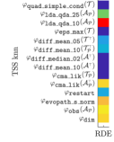

To compare the suitability of individual features as descriptors, we separated areas where the surrogate model with a particular combination has the best performance. Subseqently, we compared the distributions of each feature value on the whole with a distribution of each feature value of the selected part using Kolmogorov-Smirnov test (KS test) for MSE and RDE separately. The hypothesis of distribution equality is tested at the family-wise significance level after the Holm correction. The resulting p-values summarized in Tables S9–S13 in Supplementary material and visualised in color in Figure 1 show significant differences in distribution among combinations of model settings and TSS method for the vast majority of considered features. Features from and provided the most significant differences for almost all models. For the GP models and the sample set leading to the lowest , the p-values were often even below the smallest double precision number. These features also provided very low p-values for lmm and lq model. The only exception is providing notably higher p-values for all model settings. Moreover, features calculated on -based sample sets for TSS nearest provided in most cases higher p-values than when calculated on -based. From the model point of view, differences of RF model settings are much lower than the rest of settings for all the tested features. This might suggest the lower ability to distinguish between the individual RF settings maybe due to the low performance of these settings on the dataset. The p-values for the and the also differ notably mainly due to the different ranges of values of these two error measures. As its consequence, p-values for more clearly suggest the distinctive power of individual features on model precision, regardless the fact that is more convenient for CMA-ES related problems. Overall, the results of the KS test have shown that there is no tested landscape feature representative for which the selection of the covariance function would be negligible for the vast majority of model settings.
To perform a multivariate statistical analysis we have built two classification trees (CTs): one for TSS full and one for TSS nearest. The data for each TSS method described by 14 features selected in Subsection 3.3 were divided into 19 classes according to which of the 19 considered surrogate model settings achieved the lowest . In case of a tie, the model with the lowest among models with the lowest was the chosen one. The CT trained on those data is the MATLAB implementation of the CART (Breiman,, 1984), where the minimal number of cases in leaf was set to 5000, the twoing rule was used as a splitting criterion, was considered as a discrete variable and the remaining 13 features were considered as continuous. The resulting CTs are depicted in Figures 2 and 3.
The most successful kind of models are GPs, present in most of the leaves proving the leading role shown in pairwise comparisons of model setting errors. Gibbs and covariances of the GP models constitute the winning GP settings regardless the fact that both provided the lowest numbers of predictions (see Table 5). This is probably caused by the removal of cases where predictions of any model setting were missing. The winning model setting of RF is OC1 method being the most often selected leaf of the CT for TSS full method. The polynomial models are not present in the resulting CT for TSS nearest. The feature plays possibly the most important role in the CT for TSS full, being in the root node as well as in 4 other nodes, and also very important in the TSS nearest CT, where it is in the root node. This confirms the very strong decisive role of features indicated in the results of KS test. Basic features and in few nodes provide the decisions resulting in GP model if both feature values are small and in RF model otherwise. Such dependency coincides with the better ability of RF models to preserve the prediction quality with the growing dimension than the ability of GP models. Features from the are also very important at least in connection with the TSS nearest. The features are present only in very few nodes. We can observe the connection between the feature and the lq model in the CT for TSS full showing the possible ability of features to detect convenience of polynomial model usage.
4 Conclusion
This paper has presented a study of relationships between the prediction error of the surrogate models, their settings, and features describing the fitness landscape during evolutionary optimization by the CMA-ES state-of-the-art optimizer for expensive continuous black-box tasks. Four models in 39 different settings for the DTS-CMA-ES, a surrogate-assisted version of the CMA-ES, were compared using three sets of 14 landscape features selected according to their properties, especially according to their robustness and similarity to other features. We analysed and dependence of various models and model settings on the features calculated using three methods selecting sample sets extracted from DTS-CMA-ES runs on noiseless benchmarks from the COCO framework. Up to our knowledge, this analysis of landscape feature properties and their connection to surrogate models in evolutionary optimization is more profound than any other published so far.
Most of the landscape features were designed to be calculated on some initial sample set from the more or less uniform distribution covering the whole search space to easily identify the optimized function and/or the algorithm with the highest performance on such function. In this paper, we operate on a more local level using only data from the actual runs of the optimization algorithm generated in each generation using Gaussian distribution, i. e., data completely different from the original design of those features. Therefore, the low number of robust and mostly similar features confirms the findings of Renau et al., (2020) that the distribution of the initial design has a notable impact on landscape analysis.
The statistical analysis has shown significant differences in the error values among all 39 model settings using different TSS methods for both and . The GP model settings provided the highest perfomance followed by polynomial models. Most of the investigated features had distributions on sample sets with particular model settings achieving the lowest error values significantly different from the overall distribution of all data for both error measures and all 3 TSS methods. Finally, the overall results have shown the dispersion features as highly influential on the model settings error values, followed by features based on CMA state variables, features describing the similarity of fitness function to some simple model, features splitting space according to the black-box function values, and simple features such as dimension and number of observations.
The results of this research could be utilized to design a metalearning-based system (Kerschke et al.,, 2019; Saini et al.,, 2019) for selection of surrogate models in surrogate-assisted evolutionary optimization algorithms context. The landscape features investigated in this paper are in metalearning known as metafeatures.
References
- Auger et al., (2013) Auger, A., Brockhoff, D., and Hansen, N. (2013). Benchmarking the local metamodel CMA-ES on the noiseless BBOB’2013 test bed. GECCO ’13, pages 1225–1232.
- Auger and Hansen, (2005) Auger, A. and Hansen, N. (2005). A restart CMA evolution strategy with increasing population size. volume 2 of CEC ’05, pages 1769–1776. IEEE.
- Baerns and Holeňa, (2009) Baerns, M. and Holeňa, M. (2009). Combinatorial Development of Solid Catalytic Materials. Design of High-Throughput Experiments, Data Analysis, Data Mining. Imperial College Press / World Scientific, London.
- Bajer et al., (2019) Bajer, L., Pitra, Z., Repický, J., and Holeňa, M. (2019). Gaussian process surrogate models for the CMA Evolution Strategy. Evolutionary Computation, 27(4):665–697.
- Breiman, (1984) Breiman, L. (1984). Classification and regression trees. Chapman & Hall/CRC.
- Breiman, (2001) Breiman, L. (2001). Random forests. Machine learning, 45(1):5–32.
- Büche et al., (2005) Büche, D., Schraudolph, N. N., and Koumoutsakos, P. (2005). Accelerating evolutionary algorithms with Gaussian process fitness function models. IEEE Transactions on Systems, Man, and Cybernetics, Part C, 35(2):183–194.
- Chaudhuri et al., (1994) Chaudhuri, P., Huang, M.-C., Loh, W.-Y., and Yao, R. (1994). Piecewise-polynomial regression trees. Statistica Sinica, 4(1):143–167.
- Chen and Guestrin, (2016) Chen, T. and Guestrin, C. (2016). XGBoost: A scalable tree boosting system. KDD ’16, pages 785–794. ACM.
- Derbel et al., (2019) Derbel, B., Liefooghe, A., Verel, S., Aguirre, H., and Tanaka, K. (2019). New features for continuous exploratory landscape analysis based on the SOO tree. FOGA ’19, pages 72–86. ACM.
- Dobra and Gehrke, (2002) Dobra, A. and Gehrke, J. (2002). SECRET: A scalable linear regression tree algorithm. KDD ’02, pages 481–487. ACM.
- Flamm et al., (2002) Flamm, C., Hofacker, I. L., Stadler, P. F., and Wolfinger, M. T. (2002). Barrier Trees of Degenerate Landscapes. Zeitschrift für Physikalische Chemie International Journal of Research in Physical Chemistry and Chemical Physics, 216(2):155–173.
- Forrester and Keane, (2009) Forrester, A. and Keane, A. (2009). Recent advances in surrogate-based optimization. Progress in Aerospace Sciences, 45:50–79.
- Friedman, (2001) Friedman, J. H. (2001). Greedy function approximation: A gradient boosting machine. The Annals of Statistics, 29(5):1189–1232.
- Gibbs, (1997) Gibbs, M. N. (1997). Bayesian Gaussian Processes for Regression and Classification. PhD thesis, Department of Physics, University of Cambridge.
- Hansen, (2006) Hansen, N. (2006). The CMA evolution strategy: A comparing review. In Towards a New Evolutionary Computation, Studies in Fuzziness and Soft Comp., pages 75–102. Springer.
- Hansen, (2019) Hansen, N. (2019). A global surrogate assisted CMA-ES. GECCO ’19, pages 664–672.
- Hansen et al., (2016) Hansen, N., Auger, A., Mersmann, O., Tusar, T., and Brockhoff, D. (2016). COCO: A platform for comparing continuous optimizers in a black-box setting. arXiv:1603.08785.
- Hansen and Ostermeier, (1996) Hansen, N. and Ostermeier, A. (1996). Adapting arbitrary normal mutation distributions in evolution strategies: The covariance matrix adaptation. CEC ’96., pages 312–317. IEEE.
- Hinton and Revow, (1996) Hinton, G. E. and Revow, M. (1996). Using pairs of data-points to define splits for decision trees. In Advances in Neural Information Processing Systems, volume 8, pages 507–513. MIT Press.
- Hoos et al., (2018) Hoos, H. H., Peitl, T., Slivovsky, F., and Szeider, S. (2018). Portfolio-based algorithm selection for circuit QBFs. CP ’18, pages 195–209. Springer.
- Hosder et al., (2001) Hosder, S., Watson, L., and Grossman, B. (2001). Polynomial response surface approximations for the multidisciplinary design optimization of a high speed civil transport. Optimization and Engineering, 2:431–452.
- Jin, (2011) Jin, Y. (2011). Surrogate-assisted evolutionary computation: Recent advances and future challenges. Swarm and Evolutionary Computation, 1:61–70.
- Jin et al., (2001) Jin, Y., Olhofer, M., and Sendhoff, B. (2001). Managing approximate models in evolutionary aerodynamic design optimization. CEC ’01, pages 592–599. IEEE.
- Kern et al., (2006) Kern, S., Hansen, N., and Koumoutsakos, P. (2006). Local Meta-models for Optimization Using Evolution Strategies. PPSN ’06, pages 939–948. Springer.
- Kerschke, (2017) Kerschke, P. (2017). Comprehensive feature-based landscape analysis of continuous and constrained optimization problems using the R-package flacco. ArXiv e-prints.
- Kerschke et al., (2019) Kerschke, P., Hoos, H. H., Neumann, F., and Trautmann, H. (2019). Automated Algorithm Selection: Survey and Perspectives. Evolutionary Computation, 27(1):3–45.
- Kerschke et al., (2014) Kerschke, P., Preuss, M., Hernández, C., Schütze, O., Sun, J.-Q., Grimme, C., Rudolph, G., Bischl, B., and Trautmann, H. (2014). Cell mapping techniques for exploratory landscape analysis. EVOLVE V, pages 115–131. Springer.
- Kerschke et al., (2015) Kerschke, P., Preuss, M., Wessing, S., and Trautmann, H. (2015). Detecting funnel structures by means of exploratory landscape analysis. GECCO ’15, pages 265–272.
- Kruisselbrink et al., (2010) Kruisselbrink, J., Emmerich, M. T. M., Deutz, A., and Back, T. (2010). A robust optimization approach using Kriging metamodels for robustness approximation in the CMA-ES. CEC ’10, pages 1–8. IEEE.
- Lee et al., (2016) Lee, H., Jo, Y., Lee, D., and Choi, S. (2016). Surrogate model based design optimization of multiple wing sails considering flow interaction effect. Ocean Engineering, 121:422–436.
- Lunacek and Whitley, (2006) Lunacek, M. and Whitley, D. (2006). The dispersion metric and the CMA evolution strategy. GECCO ’06, pages 477–484.
- Mersmann et al., (2011) Mersmann, O., Bischl, B., Trautmann, H., Preuss, M., Weihs, C., and Rudolph, G. (2011). Exploratory landscape analysis. GECCO ’11, pages 829–836.
- (34) Muñoz, M. A., Kirley, M., and Halgamuge, S. K. (2015a). Exploratory landscape analysis of continuous space optimization problems using information content. IEEE Transactions on Evolutionary Computation, 19(1):74–87.
- (35) Muñoz, M. A., Sun, Y., Kirley, M., and Halgamuge, S. K. (2015b). Algorithm selection for black-box continuous optimization problems. Inf. Sci., 317(C):224–245.
- Murthy et al., (1994) Murthy, S. K., Kasif, S., and Salzberg, S. (1994). A system for induction of oblique decision trees. J. Artif. Int. Res., 2(1):1–32.
- Myers et al., (2009) Myers, R., Montgomery, D., and Anderson-Cook, C. (2009). Response Surface Methodology: Process and Product Optimization Using Designed Experiments. John Wiley & Sons, Hob.
- Pitra et al., (2016) Pitra, Z., Bajer, L., and Holeňa, M. (2016). Doubly trained evolution control for the Surrogate CMA-ES. PPSN ’16, pages 59–68. Springer.
- Pitra et al., (2017) Pitra, Z., Bajer, L., Repický, J., and Holeňa, M. (2017). Overview of surrogate-model versions of covariance matrix adaptation evolution strategy. GECCO ’17, pages 1622–1629.
- Pitra et al., (2021) Pitra, Z., Hanuš, M., Koza, J., Tumpach, J., and Holeňa, M. (2021). Interaction between model and its evolution control in surrogate-assisted CMA evolution strategy. GECCO ’21, pages 528–536.
- Pitra et al., (2018) Pitra, Z., Repický, J., and Holeňa, M. (2018). Boosted regression forest for the doubly trained surrogate covariance matrix adaptation evolution strategy. ITAT ’18, pages 72–79. CEUR.
- Pitra et al., (2019) Pitra, Z., Repický, J., and Holeňa, M. (2019). Landscape analysis of Gaussian process surrogates for the covariance matrix adaptation evolution strategy. GECCO ’19, pages 691–699.
- Rasheed et al., (2005) Rasheed, K., Ni, X., and Vattam, S. (2005). Methods for using surrogate models to speed up genetic algorithm oprimization: Informed operators and genetic engineering. In Knowledge Incorporation in Evolutionary Computation, pages 103–123. Springer.
- Rasmussen and Williams, (2006) Rasmussen, C. E. and Williams, C. K. I. (2006). Gaussian Processes for Machine Learning. MIT Press.
- Renau et al., (2020) Renau, Q., Doerr, C., Dréo, J., and Doerr, B. (2020). Exploratory landscape analysis is strongly sensitive to the sampling strategy. PPSN ’20, pages 139–153. Springer.
- Renau et al., (2019) Renau, Q., Dréo, J., Doerr, C., and Doerr, B. (2019). Expressiveness and robustness of landscape features. GECCO ’19, pages 2048–2051.
- Renau et al., (2021) Renau, Q., Dréo, J., Doerr, C., and Doerr, B. (2021). Towards explainable exploratory landscape analysis: Extreme feature selection for classifying BBOB functions. EvoStar ’21, pages 17–33.
- Saini et al., (2019) Saini, B. S., Lopez-Ibanez, M., and Miettinen, K. (2019). Automatic surrogate modelling technique selection based on features of optimization problems. GECCO ’19, pages 1765–1772.
- Schweizer and Wolff, (1981) Schweizer, B. and Wolff, E. F. (1981). On nonparametric measures of dependence for random variables. Annals of Statistics, 9(4):879–885.
- Zaefferer et al., (2016) Zaefferer, M., Gaida, D., and Bartz-Beielstein, T. (2016). Multi-fidelity modeling and optimization of biogas plants. Applied Soft Computing, 48:13–28.