Faster Asynchronous Nonconvex Block Coordinate
Descent with Locally Chosen Stepsizes

Abstract

Distributed nonconvex optimization problems underlie many applications in learning and autonomy, and such problems commonly face asynchrony in agents’ computations and communications. When delays in these operations are bounded, they are called partially asynchronous. In this paper, we present an uncoordinated stepsize selection rule for partially asynchronous block coordinate descent that only requires local information to implement, and it leads to faster convergence for a class of nonconvex problems than existing stepsize rules, which require global information in some form. The problems we consider satisfy the error bound condition, and the stepsize rule we present only requires each agent to know (i) a certain type of Lipschitz constant of its block of the gradient of the objective and (ii) the communication delays experienced between it and its neighbors. This formulation requires less information to be available to each agent than existing approaches, typically allows for agents to use much larger stepsizes, and alleviates the impact of stragglers while still guaranteeing convergence to a stationary point. Simulation results provide comparisons and validate the faster convergence attained by the stepsize rule we develop.

I Introduction

A number of applications in learning and autonomy take the form of distributed optimization problems in which a network of agents minimizes a global objective function $f$. As these problems grow in size, asynchrony may result from delays in computations and communications between agents. For many problems (i.e., those such that $\nabla^{2}f$ is not block-diagonally dominant [1, Theorem 4.1(c)]), arbitrarily long delays may cause the system to fail to converge [2, Chapter 7, Example 1.3]. Synchrony can be enforced by making faster agents idle while waiting for communications from slower agents, though the network will suffer from “straggler” slowdown, where the progress of the network is restricted by its slowest agent. This has led to interest in partially asynchronous algorithms, which converge to a solution when all delays in communications and computations are bounded by a known upper limit $B$ [3, 4].

Partially asynchronous algorithms avoid requiring agents to idle by instead “damping” the dynamics of the system based on knowledge of $B$. For gradient-based algorithms, this is achieved by reducing agents’ stepsize $\gamma$ as $B$ grows. While this method (along with mild assumptions on $f$) ensures convergence when all delays are bounded by $B$, straggler slowdown is still present. Specifically, in existing block coordinate descent algorithms, if just one agent’s delays have length up to $B$, then every agent’s stepsize is $O(1/B)$, even if the delays experienced by the other agents are much shorter than $B$ [5, 4, 3]. When $B$ is large, this method leads to excessively small stepsizes, which significantly slow convergence. This stepsize rule also requires agents to have knowledge of $B$, which may be difficult to gain. For example, agents in a large network may not know the lengths of all delays experienced by all agents.

In this paper, we will instead show that, under the same standard assumptions on $f$ in seminal work in [3], a gradient-based partially asynchronous algorithm converges to a solution while allowing agents to choose uncoordinated stepsizes using only local information. That is, agent $i$ may choose its own stepsize $\gamma_{i}$ as a function of only a few entries of $\nabla f$ and only the communication delays between itself and its neighbors. We analyze block coordinate descent because it is widely used and because it is a building block for many other algorithms. In this and related algorithms, the stepsize is the only free parameter and it has a substantial impact on convergence rate, which makes the use of larger values essential when possible. We prove that agents still converge to a stationary point under this new stepsize rule, and comparisons in simulation validate the significant speedup that we attain. To the best of the authors’ knowledge, this is the first proof of convergence of a partially asynchronous algorithm with uncoordinated stepsizes chosen using only local information.

Related work in [6, 7, 8, 9, 10, 11] allows for uncoordinated stepsizes that differ across agents, though they must still obey a bound computed with global information. In contrast, in this paper each agent’s stepsize bound can be computed using only local information, i.e., global Lipschitz constants and global delay bounds are not required, hence the “locally chosen” label. Existing literature with locally chosen stepsizes either requires a synchronous setting [12], diminishing stepsizes [13, 14], or for $\nabla^{2}f$ to be block diagonally-dominant [15], whereas we do not require any of these.

The rest of the paper is organized as follows. Section II gives the problems and algorithm we study. Then Section III proves convergence under the local stepsize rule we develop and gives a detailed discussion of our developments in relation to recent work. Section IV empirically verifies the speedup we attain, and finally Section V concludes.

II Problem Statement and Preliminaries

This section establishes the problems we solve, the assumptions placed on them, and the algorithm we use. Below, we use the notation $[d]=\{1,\ldots,d\}$ for $d\in\mathbb{N}$.

II-A Problem Statement and Assumptions

We solve problems of the following form:

Problem 1

Given $N$ agents, a function $f:\mathbb{R}^{n}\to\mathbb{R}$, and a set $X\subseteq\mathbb{R}^{n}$, asynchronously solve

$$\underset{x\in X}{\textnormal{minimize}}\,\,f(x). \triangle$$

We first make the following assumption about $X$:

Assumption 1

There exist sets $X_{1},\ldots,X_{N}$ such that $X=X_{1}\times X_{2}\times\dots\times X_{N}$, where $X_{i}\subseteq\mathbb{R}^{n_{i}}$ is nonempty, closed, and convex for all $i\in[N]$, and $n=\sum_{i\in[N]}n_{i}$. $\triangle$

We emphasize that $X$ need not be compact, e.g., it can be all of $\mathbb{R}^{n}$. This decomposition will allow each agent to execute a projected gradient update law asynchronously and still ensure set constraint satisfaction. For any closed, convex set $\Omega$, we use $\Pi_{\Omega}[y]$ to denote the Euclidean projection of $y$ onto $\Omega$.

In our analysis, we will divide $n$-dimensional vectors into $N$ blocks. Given a vector $v\in\mathbb{R}^{n}$, where $n=\sum_{i=1}^{N}n_{i}$, the $i^{th}$ block of $v$, denoted $v^{[i]}$, is the $n_{i}$-dimensional vector formed by entries of $v$ with indices $\sum_{k=1}^{i-1}n_{k}+1$ through $\sum_{k=1}^{i}n_{k}$. In other words, $v^{[1]}$ is the first $n_{1}$ entries of $v$, $v^{[2]}$ is the next $n_{2}$ entries, etc. Thus, for $x\in X$, we have $x^{[k]}\in X_{k}$ for all $k\in[N]$. For $\nabla f(x)$, we write $\nabla^{[1]}f(x)$ for its first $n_{1}$ entries, $\nabla^{[2]}f(x)$ for its next $n_{2}$ entries, etc.

We assume the following about $f$.

Assumption 2

$f$ is bounded from below on $X$. $\triangle$

Assumption 3

$f$ is $L^{i}_{j}$-smooth on $X$. That is, for all $i,j\in[N]$ and for any $x,y\in X$ with $x^{[k]}=y^{[k]}$ for all $k\neq j$, there exists a constant $L^{i}_{j}\geq 0$ such that $\|\nabla^{[i]}f(x)-\nabla^{[i]}f(y)\|\leq L^{i}_{j}\|x^{[j]}-y^{[j]}\|$. $\triangle$

In words, each block of $\nabla f$ must be Lipschitz in each block of its argument. We note that any $L$-smooth function $f$ in the traditional sense (i.e., satisfying $\|\nabla f(x)-\nabla f(y)\|\leq L\|x-y\|$ for all $x,y\in X$) trivially satisfies Assumption 3 by setting $L^{i}_{j}=L$ for all $i,j\in[N]$. Thus, Assumption 3 is no stronger than the standard $L$-smooth assumption, but it will allow us to leverage more fine-grained information from the problem. Note also from this construction that $L^{i}_{j}=L^{j}_{i}$.

II-B Algorithm Setup

For all $i\in[N]$, agent $i$ stores a local copy of $x$, denoted $x_{i}$. Due to asynchrony, we can have $x_{i}\neq x_{j}$ for $i\neq j$. Agent $i$ is tasked with updating the $i^{th}$ block of the decision variable, and thus it performs computations on its own block $x^{[i]}_{i}$. For $j\neq i$, agent $i$’s copy of agent $j$’s block, denoted $x_{i}^{[j]}$, only changes when it receives a communication from agent $j$.

Due to asynchrony in communications, at time $t$ we expect $x^{[j]}_{i}(t)\neq x^{[j]}_{j}(t)$. We define the term $\tau^{j}_{i}(t)$ to be the largest time index such that $\tau^{j}_{i}(t)\leq t$ and $x^{[j]}_{i}(t)=x^{[j]}_{j}(\tau^{j}_{i}(t))$. In words, $\tau^{j}_{i}(t)$ is the most recent time at which $x^{j}_{j}$ equaled the value of $x^{i}_{j}(t)$. Note that $\tau^{i}_{i}(t)=t$ for all $i\in[N]$. Using this notation, for all $i\in[N]$, we may write agent $i$’s local copy of $x$ as ${x_{i}(t)=(x^{[1]}_{1}(\tau^{1}_{i}(t)),\dots,x^{[n]}_{n}(\tau^{n}_{i}(t))}$.

Defining $T^{i}$ as the set of all time indices for which agent $i$ computes an update to $x^{[i]}_{i}$, we formalize the partially asynchronous block coordinate descent algorithm as follows.

Algorithm 1: Let $f$, $X$, $x_{1}(0),\ldots,x_{N}(0)$, and $\gamma_{1},\ldots,\gamma_{N}>0$ be given. For all $i\in[N]$ and $j\in[N]\backslash\{i\}$, execute

$$x_{i}^{[i]}(t+1) =\begin{cases}\Pi_{X_{i}}\left[x_{i}^{[i]}(t)-\gamma_{i}\nabla^{[i]}f(x_{i}(t))\right]&t\in T^{i}\\ x_{i}^{[i]}(t)&t\notin T^{i}\end{cases}$$

$$x_{j}^{[i]}(t\!+\!1) =\begin{cases}x_{j}^{[j]}\left(\tau_{i}^{j}(t\!+\!1)\right)&\text{$i$ receives~{}$x^{[j]}_{j}$ at time~{}$t\!+\!1$}\\ x_{j}^{[i]}(t)&\text{otherwise.}\hfill\diamond\end{cases}$$

We emphasize that agents do not need to know $T^{i}$ or $\tau^{j}_{i}$ for any $i$ or $j$; these are only used in our analysis. Additionally, communications in Algorithm 1 are generally not all-to-all; agents $i$ and $j$ only need to communicate if $\nabla^{[i]}f$ has an explicit dependence on agent $j$’s block (i.e., if $L^{i}_{j}\neq 0$).

Below, we will analyze the “true” state of the network, denoted $x(t)=(x^{[1]}_{1}(t),\dots,x^{[n]}_{n}(t))$, which contains each agent’s current value of its own block. For clarity we will write $x^{[i]}(t)$ when discussing the $i^{th}$ block of the global state $x(t)$, and we will write $x^{[i]}_{i}(t)$ when discussing the $i^{th}$ block of agent $i$’s local copy $x_{i}(t)$, though we note that $x^{[i]}(t)=x^{[i]}_{i}(t)$ by definition.

Partial asynchrony is enforced by the next two assumptions

Assumption 4

For every $i,j\in[N]$, there exists an integer $D^{j}_{i}\geq 0$ such that $0\leq t^{i}-\tau^{j}_{i}(t^{i})\leq D^{j}_{i}$ for all $t^{i}\in T^{i}$. $\triangle$

Assumption 4 states that when agent $i$ computes an update, its value of agent $j$’s block equals some value that $x^{[j]}_{j}$ had at some point in the last $D^{j}_{i}+1$ timesteps. Note that $D^{i}_{i}=0$, and we allow $D^{j}_{i}\neq D^{i}_{j}$, i.e., delays not need be symmetric for any pair of agents. For completeness, if two agents $i$ and $j$ do not communicate (i.e., $L^{i}_{j}=0$), then $D^{i}_{j}=D^{j}_{i}=0$.

Assumption 5

For each $i\in[N]$, there exists an integer $G_{i}\geq 0$ such that for every $t$, $T^{i}\cap\{t,t+1,\dots,t+G_{i}\}\neq\emptyset$. $\triangle$

Assumption 5 simply states that agent $i$ updates at least once every $G_{i}+1$ timesteps. Note that in the existing partially asynchronous literature $B=\max_{i,j\in[N]}\{D^{j}_{i},D^{i}_{j},G_{i}\}$, and this is used to calibrate stepsizes. We show in the next section that a finer-grained analysis leads to local stepsize rules that still ensure convergence.

III Convergence Results

The goal of Algorithm 1 is to find an element of the solution set $X^{*}:=\{x\in X:x=\Pi_{X}\left[x-\nabla f(x)\right]\}$. That is, we wish to show $\lim_{t\rightarrow\infty}\|x(t)-x^{*}\|=0$, where $x^{*}$ is some element of $X^{*}$. Our proof strategy is to first establish that the sequence $\{x(t)\}^{\infty}_{t=0}$ has square summable successive differences, then show that its limit point is indeed an element of $X^{*}$.

III-A Analysis of Algorithm 1

The forthcoming theorem uses the following lemma.

Lemma 1

Let Assumption 3 hold. For all $i\in[N]$ and $x,y\in X$, $\|\nabla^{[i]}f(x)-\nabla^{[i]}f(y)\|\leq\sum_{j=1}^{N}L^{i}_{j}\|x^{[j]}-y^{[j]}\|$.

Proof: Fix $x,y\in X$. For all $k\in\{0,\dots,N\}$, define a vector $z_{k}\in\mathbb{R}^{n}$ as $z^{[j]}_{k}=x^{[j]}$ if $j>k$ and $z^{[j]}_{k}=y^{[j]}$ if $j\leq k$. By this definition, $z_{0}=x$ and $z_{N}=y$. Then $\|\nabla^{[i]}f(x)-\nabla^{[i]}f(y)\|=\|\sum_{k=1}^{N}\nabla^{[i]}f(z_{k-1})-\nabla^{[i]}f(z_{k})\|\leq\sum_{k=1}^{N}\|\nabla^{[i]}f(z_{k-1})-\nabla^{[i]}f(z_{k})\|.$ We note that $z_{k-1}$ and $z_{k}$ differ in only one block, i.e., $z_{k-1}^{[j]}=z_{k}^{[j]}$ for all $j\neq k$, and $z_{k-1}^{[k]}\neq z_{k}^{[k]}$. Then each element of the sum satisfies the conditions of Assumption 3, and applying it to each element of the sum completes the proof. $\hfill\blacksquare$

For conciseness, we define $s(t)=x(t+1)-x(t)$. The following theorem shows that the sequence $\{s(t)\}^{\infty}_{t=0}$ decays to zero.

Theorem 1

Let Assumptions 1-5 hold. If for all ${i\in[N]}$ we have $\gamma_{i}\in\left(0,\frac{2}{\sum_{j=1}^{N}L^{i}_{j}(1+D^{j}_{i}+D^{i}_{j})}\right)$, then under Algorithm 1 we have $\lim_{t\rightarrow\infty}\|x(t+1)-x(t)\|=0$ and, for all $i\in[N]$, $\lim_{t\rightarrow\infty}\|x(t)-x_{i}(t)\|=0$.

Proof: See Appendix A. $\hfill\blacksquare$

III-B Convergence of Algorithm 1 to a Stationary Point

Theorem 1 on its own does not necessarily guarantee that Algorithm 1 converges to an element of $X^{*}$, and in order to do so we must impose additional assumptions on $f$. The first is the error bound condition.

Assumption 6 ([16])

For every $\alpha>0$, there exist $\delta,\kappa>0$ such that for all $x\in X$ with $f(x)\leq\alpha$ and $\|x-\Pi_{X}\left[x-\nabla f(x)\right]\|\leq\delta$,

$$\min_{\bar{x}\in X^{*}}\|x-\bar{x}\|\leq\kappa\|x-\Pi_{X}\left[x-\nabla f(x)\right]\|. \triangle$$

Assumption 6 is satisfied by a number of problems, including several classes of non-convex problems [17, 18]. It also holds when $f$ is strongly convex on $X$ or satisfies the quadratic growth condition on $X$ [17, 18], and when $X$ is polyhedral and $f$ is either quadratic [16] or the dual functional associated with minimizing a strictly convex function subject to linear constraints [19].

Additionally, we make the following assumption on $X^{*}$, which simply states that the elements of $X^{*}$ are isolated and sufficiently separated from each other.

Assumption 7

There exists a scalar $\epsilon>0$ such that for every distinct $x,y\in X^{*}$ we have $\|x-y\|\geq\epsilon$. $\triangle$

In addition to Assumptions 6 and 7, we will utilize the following lemma.

Lemma 2

For any $x\in X$, any $i\in[N]$, and any $\gamma_{i}>0$,

$$\left\|x^{[i]}(t)-\Pi_{X_{i}}\left[x^{[i]}(t)-\nabla^{[i]}f(x(t))\right]\right\|\leq\max\left\{1,\frac{1}{\gamma_{i}}\right\}\left\|x^{[i]}(t)-\Pi_{X_{i}}\left[x^{[i]}(t)-\gamma_{i}\nabla^{[i]}f(x(t))\right]\right\|.$$ (1)

Proof: This follows from [3, Lemma 3.1] with $\gamma_{i}$, $x^{[i]}(t)$, $\nabla^{[i]}f(x(t))$, and $X_{i}$ replacing $\gamma,x,\nabla f$, and $X$. $\blacksquare$

Theorem 2

Let the conditions of Theorem 1 and Assumptions 6 and 7 hold. Then, for some $x^{*}\in X^{*}$,

$$\lim_{t\rightarrow\infty}\|x(t)-x^{*}\|=0.$$ (2)

Proof: For every $t$ and $i\in[N]$, define $k_{i}(t)=\hat{t}_{i}$, where $\hat{t}_{i}$ is the largest element of $T^{i}$ such that $\hat{t}_{i}\leq t$. By Assumption 5, $k_{i}(t)\geq t-G_{i}$ for all $t$. Therefore, as $t\rightarrow\infty$, $k_{i}(t)\rightarrow\infty$, which, under Theorem 1, gives $\lim_{t\rightarrow\infty}\|s^{[i]}(k_{i}(t))\|=0$ for all $i\in[N]$. The definition of $s^{[i]}$ and Algorithm 1 give

$$s^{[i]}(k_{i}(t))=\Pi_{X_{i}}\left[x^{[i]}(k_{i}(t))-\gamma_{i}\nabla^{[i]}f(x_{i}(k_{i}(t)))\right]-x^{[i]}(k_{i}(t)).$$ (3)

We now define the residual vector $r^{[i]}(k_{i}(t))$ as

$$r^{[i]}(k_{i}(t))=\Pi_{X_{i}}\left[x^{[i]}(k_{i}(t))-\gamma_{i}\nabla^{[i]}f(x(k_{i}(t)))\right]-x^{[i]}(k_{i}(t))$$ (4)

for all $i\in[N]$. Note that the arguments of the gradient term differ between $s^{[i]}$ and $r^{[i]}$. Here, $s^{[i]}$ represents the update performed by agent $i$ with its asynchronous information, while $r^{[i]}$ represents the update that agent $i$ would take if it had completely up to date information from its neighbors. The non-expansive property of $\Pi_{X_{i}}$ gives

$$\|s^{[i]}(k_{i}(t))-r^{[i]}(k_{i}(t))\| \leq\gamma_{i}\|\nabla^{[i]}f(x(k_{i}(t)))-\nabla^{[i]}f(x_{i}(k_{i}(t)))\|$$ (5)

$$\leq\gamma_{i}\sum_{j=1}^{N}L^{i}_{j}\|x^{[j]}(k_{i}(t))-x^{[j]}_{i}(k_{i}(t))\|,$$ (6)

where the last line follows from Lemma 1.

Theorem 1 gives $\lim_{t\rightarrow\infty}\|x^{[j]}(t)-x^{[j]}_{i}(t)\|=0$ for all $i,j\in[N]$, implying $\lim_{t\rightarrow\infty}\|x^{[j]}(k_{i}(t))-x^{[j]}_{i}(k_{i}(t))\|=0$. Combined with (6), this gives $\lim_{t\rightarrow\infty}\|s^{[i]}(k_{i}(t))-r^{[i]}(k_{i}(t))\|=0$. Because $\lim_{t\rightarrow\infty}\|s^{[i]}(k_{i}(t))\|=0$, we have $\lim_{t\rightarrow\infty}\|r^{[i]}(k_{i}(t))\|=0$ for all $i\in[N]$ and therefore $\lim_{t\rightarrow\infty}\|r^{[i]}(t)\|=0$. Using Lemma 2, we have

$$\|x(t)-\Pi_{X}\left[x(t)-\nabla f(x(t))\right]\| \leq\sum^{N}_{i=1}\left\|x^{[i]}(t)-\Pi_{X_{i}}\left[x^{[i]}(t)-\nabla^{[i]}f(x(t))\right]\right\|$$ (7)

$$\leq\sum^{N}_{i=1}\max\left\{1,\frac{1}{\gamma_{i}}\right\}\left\|x^{[i]}(t)-\Pi_{X_{i}}\left[x^{[i]}(t)-\gamma_{i}\nabla^{[i]}f(x(t))\right]\right\|$$ (8)

$$=\sum^{N}_{i=1}\max\left\{1,\frac{1}{\gamma_{i}}\right\}\|r^{[i]}(t)\|,$$ (9)

implying $\lim_{t\rightarrow\infty}\|x(t)-\Pi_{X}\left[x(t)-\nabla f(x(t))\right]\|=0$. Since $\{f(x(t))\}_{t=1}^{\infty}$ is bounded by Theorem 1, then by Assumption 6 there exists a threshold $\bar{t}\geq 0$ and scalar $\kappa>0$ such that

$$\min_{\bar{x}\in X^{*}}\|x(t)-\bar{x}\|\leq\kappa\|x(t)-\Pi_{X}\left[x(t)-\nabla f(x(t))\right]\|$$ (10)

for all $t\geq\bar{t}$. For each $t$, let $\bar{x}(t)=\arg\min_{\bar{x}\in X^{*}}\|x(t)-\bar{x}\|$. Then, combining (10) with (9) gives $\lim_{t\rightarrow\infty}\|x(t)-\bar{x}(t)\|=0$, which along with Theorem 1 implies $\lim_{t\rightarrow\infty}\|\bar{x}(t+1)-\bar{x}(t)\|=0$. Then Assumption 7 implies that there exists a $\hat{t}\geq\bar{t}$ such that $\bar{x}(t)=x^{*}$ for all $t\geq\hat{t}$, where $x^{*}=\bar{x}(\hat{t})$. This gives $\lim_{t\rightarrow\infty}\|x(t)-x^{*}\|=0$, as desired. $\hfill\blacksquare$

III-C Comparison to Existing Works

We make a few remarks on the two preceding theorems.

Remark 1

Our locally chosen stepsize rule given in Theorem 1 improves on the one provided in [4], which is the most relevant work, in a few ways. For clarity, our rule is

$$\gamma_{i}\in\left(0,\frac{2}{\sum_{j=1}^{N}L^{i}_{j}(1+D^{j}_{i}+D^{i}_{j})}\right)\text{ for all }i\in[N],$$ (11)

while the global, coordinated rule in [4] is

$$\gamma\in\left(0,\frac{2}{L(1+2\sqrt{N}B)}\right).$$ (12)

First, while the similarity in structure between  (11) and (12) is evident, (11) only requires agent $i$ to know $\nabla^{[i]}f$ and the inward and outward communication delays to and from its neighbors to compute $\gamma_{i}$. Second, the $\sqrt{N}$ in (12) is eliminated. The elimination of this explicit dependence on $B$ and $N$ is significant, especially when $B$ is large compared to the communication delays experienced by a particular agent, and $N$ is large compared to the number of neighbors a particular agent communicates with, in which case the upper bound in (11) will be significantly larger than in (12).

Remark 2

Under Assumptions 1-7, our stepsize rule can be shown to provide geometric convergence by following a similar argument to [3] and [4]. However, (as seen in [3] and [4]) a convergence rate proof is quite involved, and due to space constraints is deferred to a future publication. Thus, to reiterate, the contribution of this paper is providing, to the best of the authors’ knowledge, the first proof of convergence of a partially asynchronous algorithm with uncoordinated stepsizes chosen using only local information.

IV Simulations

We compare the performance of the locally chosen stepsize rule (11) with the globally coordinated rule (12) on a set-constrained quadratic program of the form $f(x)=\frac{1}{2}x^{T}Qx+r^{T}x$. There are $N=20$ agents, each of which updates a scalar variable. $Q$ and $r$ are generated such that $Q\nsucceq 0$, $n=20$, $L=100$, and $X_{i}=\{x\in\mathbb{R}:|x|\leq 10,000\}$ for all $i\in[N]$. Under this setup, $f$ is a nonconvex quadratic function on a polyhedral constraint set $X$, which satisfies Assumption 6 [16]. Each communication bound $D^{j}_{i}$ is randomly chosen from $\{0,\dots,20\}$.

Since the effect of asynchronous communications is maximized when communications are less frequent than computations, we have every agent compute an update at every timestep, i.e., $T_{i}=\mathbb{N}$ for all $i\in[N]$. In this simulation communications between agents are instantaneous, with asynchrony arising from them being infrequent, with the number of timesteps between communications from agent $j$ to agent $i$ being bounded by $D^{j}_{i}$. If agent $j$ communicates with agent $i$ at time $t$, the next such communication will occur at $t+1+\delta^{j}_{i}(t)$, where $\delta^{j}_{i}(t)$ is a randomly chosen element of $\{0,\dots,D^{j}_{i}\}$. This simulation is run from $t=0$ to $t=500$, and every agent is initialized with $x_{i}(0)=0$.

To ensure a fair comparison, both simulations are run using the same communication and computation time indices; one using a global coordinated stepsize, and the other using locally chosen stepsizes. The global coordinated stepsize is chosen to be the upper bound in (12) multiplied by 0.95 (to satisfy the strict inequality), which gives $\gamma=2.1\times 10^{-4}$. The local stepsizes are chosen as the upper bounds in (11) multiplied by 0.95, and range from $4.9\times 10^{-4}$ to $2.8\times 10^{-3}$. The values of $f(x(t))$ for each simulation are plotted against $t$ in Figure 1, where a clear speedup in convergence can be seen.

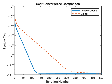
Figure 1: Convergence comparison of $f(x(t))$ for algorithms using globally chosen (12) (orange dashed line) and locally chosen (11) (blue solid line) stepsizes. (12) is to the best of the authors’ knowledge the best available result in the literature, and the stepsize rule developed in this paper is shown to significantly accelerate convergence beyond it.

In Figure 1, we can see that both stepsize schemes appear to achieve geometric convergence, with our locally chosen scheme reaching a solution significantly faster. In particular, the algorithm using locally chosen stepsizes converges to a stationary point and stops updating at $t=239$, while the algorithm using a global stepsize is still updating as of $t=500$. This illustrates better performance when using the stepsize rule presented in this paper compared to the current state of the art, in addition to allowing the agents to implement this rule using only local information.

V Conclusions

We have presented, to the best of the authors’ knowledge, the first proof of convergence of a partially asynchronous algorithm with uncoordinated stepsizes chosen using only local information. The local stepsize selection rule in this paper generally allows for larger stepsizes than the current state of the art and is empirically shown to significantly accelerate convergence. Future work will develop a full proof of geometric convergence of Algorithm 1 and extend this stepsize rule to other algorithms.

Appendix A Proof of Theorem 1

In addition to Lemma 1, proof of Theorem 1 will use the following lemmas:

Lemma 3

Under Assumption 1, for all $t$ and all $i\in[N]$ in Algorithm 1 we have $\langle s^{[i]}(t),\nabla^{[i]}f(x_{i}(t))\rangle\leq-\frac{1}{\gamma_{i}}\|s^{[i]}(t)\|^{2}$.

Proof: This is a property of orthogonal projections [3]. $\blacksquare$

Lemma 4

Consider the set $\{0,\dots,M\}$, with $M\leq\infty$. Then $\sum_{i=0}^{M}\sum_{j=0}^{M}a^{j}_{i}=\sum_{i=0}^{M}\sum_{j=0}^{M}a^{i}_{j}$

Proof: This follows by re-labeling indices. $\blacksquare$

Proof of Theorem 1: The identities $x(t+1)=x(t)+s(t)$ and $f(a)-f(b)=\int^{1}_{0}\langle(a-b),\nabla f(b+\tau(a-b))\rangle d\tau$ give

$$f(x(t+1))-f(x(t)) =\int^{1}_{0}\langle s(t),\nabla f(x(t)+\tau s(t)\rangle d\tau$$ (13)

$$=\sum_{i=1}^{N}\int^{1}_{0}\langle s^{[i]}(t),\nabla^{[i]}f(x(t)+\tau s(t))\rangle d\tau$$ (14)

$$=\sum_{i=1}^{N}\langle s^{[i]}(t),\nabla^{[i]}f(x_{i}(t))\rangle+H_{i}(t)$$ (15)

$$\leq\sum_{i=1}^{N}-\frac{1}{\gamma_{i}}\|s^{[i]}(t)\|^{2}+H_{i}(t),$$ (16)

where the last line uses Lemma 3 and $H_{i}(t)=\int^{1}_{0}\langle s^{[i]}(t),\nabla^{[i]}f(x(t)+\tau s(t))-\nabla^{[i]}f(x_{i}(t))\rangle d\tau$. Next,

$$H_{i}(t) \leq\int^{1}_{0}\|s^{[i]}(t)\|\|\nabla^{[i]}f(x(t)+\tau s(t))-\nabla^{[i]}f(x_{i}(t))\|d\tau$$ (17)

$$\leq\|s^{[i]}(t)\|\sum_{j=1}^{N}L^{i}_{j}\int^{1}_{0}\|x^{[j]}(t)+\tau s^{[j]}(t)-x^{[j]}_{i}(t)\|d\tau$$ (18)

$$\leq\|s^{[i]}(t)\|\sum_{j=1}^{N}L^{i}_{j}\int^{1}_{0}\left(\tau\|s^{[j]}(t)\|+\|x^{[j]}(t)-x^{[j]}_{i}(t)\|\right)d\tau$$ (19)

$$=\|s^{[i]}(t)\|\sum_{j=1}^{N}L^{i}_{j}\left(\frac{1}{2}\|s^{[j]}(t)\|+\|x^{[j]}(t)-x^{[j]}_{i}(t)\|\right),$$ (20)

where the $2^{nd}$ line uses Lemma 1. Using $ab\leq\frac{a^{2}+b^{2}}{2}$ gives

$$\|s^{[i]}(t)\|\sum_{j=1}^{N}L^{i}_{j}\frac{1}{2}\|s^{[j]}(t)\|\leq\frac{1}{2}\sum_{j=1}^{N}L^{i}_{j}\left(\frac{1}{2}\|s^{[i]}(t)\|^{2}+\frac{1}{2}\|s^{[j]}(t)\|^{2}\right).$$ (21)

To bound the term $\|s^{[i]}(t)\|\sum_{j=1}^{N}L^{i}_{j}\|x^{[j]}(t)-x^{[j]}_{i}(t)\|$ in (20), recall that $x^{[j]}(t)=x^{[j]}_{j}(t)$ and $x^{[j]}_{i}(t)=x^{[j]}_{j}(\tau^{j}_{i}(t))$. Then

$$\|x^{[j]}(t)-x^{[j]}_{i}(t)\| =\|x^{[j]}_{j}(t)-x^{[j]}_{j}(\tau^{j}_{i}(t))\|$$ (22)

$$=\left\|\sum^{t-1}_{k=\tau^{j}_{i}(t)}s^{[j]}(k)\right\|$$ (23)

$$\leq\sum^{t-1}_{k=\tau^{j}_{i}(t)}\|s^{[j]}(k)\|,$$ (24)

If $\tau^{j}_{i}(t)=t$, the above sum is $0$. Using (24) and $ab\leq\frac{a^{2}+b^{2}}{2}$, we have

$$\|s^{[i]}(t)\|\sum_{j=1}^{N}L^{i}_{j}\|x^{[j]}(t)-x^{[j]}_{i}(t)\| \leq\|s^{[i]}(t)\|\sum_{j=1}^{N}L^{i}_{j}\sum^{t-1}_{k=\tau^{j}_{i}(t)}\|s^{[j]}(k)\|$$ (25)

$$\leq\sum_{j=1}^{N}L^{i}_{j}\sum^{t-1}_{k=\tau^{j}_{i}(t)}\frac{1}{2}\left(\|s^{[i]}(t)\|^{2}+\|s^{[j]}(k)\|^{2}\right)$$ (26)

$$=\frac{1}{2}\sum_{j=1}^{N}L^{i}_{j}\left(\!(t-\tau^{j}_{i}(t))\|s^{[i]}(t)\|^{2}+\!\!\!\sum^{t-1}_{k=\tau^{j}_{i}(t)}\!\!\|s^{[j]}(k)\|^{2}\!\right)$$ (27)

$$\leq\frac{1}{2}\sum_{j=1}^{N}L^{i}_{j}\left(D^{j}_{i}\|s^{[i]}(t)\|^{2}+\sum^{t-1}_{k=\tau^{j}_{i}(t)}\|s^{[j]}(k)\|^{2}\right),$$ (28)

where the last line follows from Assumption 4. Using (21) and (28) in (20) gives

$$H_{i}(t)\leq\frac{1}{2}\sum_{j=1}^{N}L^{i}_{j}\left(\frac{1}{2}+D^{j}_{i}\right)\|s^{[i]}(t)\|^{2}+\frac{1}{2}\sum_{j=1}^{N}L^{i}_{j}\left(\frac{1}{2}\|s^{[j]}(t)\|^{2}+\sum^{t-1}_{k=\tau^{j}_{i}(t)}\|s^{[j]}(k)\|^{2}\right),$$ (29)

which combined with (16) gives

$$f(x(t\!+\!1))-f(x(t))\leq\sum_{i=1}^{N}\!\left(\!-\frac{1}{\gamma_{i}}\!+\!\frac{1}{2}\sum_{j=1}^{N}L^{i}_{j}\left(\frac{1}{2}\!+\!D^{j}_{i}\right)\right)\|s^{[i]}(t)\|^{2}+\sum^{N}_{i=1}\frac{1}{2}\sum_{j=1}^{N}L^{i}_{j}\left(\frac{1}{2}\|s^{[j]}(t)\|^{2}+\sum^{t-1}_{k=\tau^{j}_{i}(t)}\|s^{[j]}(k)\|^{2}\right).$$ (30)

From Lemma 4, we see

$$\sum^{N}_{i=1}\frac{1}{2}\sum_{j=1}^{N}L^{i}_{j}\left(\frac{1}{2}\|s^{[j]}(t)\|^{2}+\sum^{t-1}_{k=\tau^{j}_{i}(t)}\|s^{[j]}(k)\|^{2}\right)=\sum^{N}_{i=1}\frac{1}{2}\sum_{j=1}^{N}L^{j}_{i}\left(\frac{1}{2}\|s^{[i]}(t)\|^{2}+\sum^{t-1}_{k=\tau^{i}_{j}(t)}\|s^{[i]}(k)\|^{2}\right),$$ (31)

which, using the fact that $L^{i}_{j}=L^{j}_{i}$, gives

$$f(x(t+1))-f(x(t))\leq\sum_{i=1}^{N}\left(-\frac{1}{\gamma_{i}}+\frac{1}{2}\sum_{j=1}^{N}L^{i}_{j}\left(1+D^{j}_{i}\right)\right)\|s^{[i]}(t)\|^{2}+\sum^{N}_{i=1}\frac{1}{2}\sum_{j=1}^{N}L^{i}_{j}\sum^{t-1}_{k=\tau^{i}_{j}(t)}\|s^{[i]}(k)\|^{2}.$$ (32)

Summing this inequality over $t$ from $0$ to $m-1$ and rearranging gives

$$f(x(m))-f(x(0))\leq\sum_{i=1}^{N}\left(-\frac{1}{\gamma_{i}}+\frac{1}{2}\sum_{j=1}^{N}L^{i}_{j}\left(1+D^{j}_{i}\right)\right)\sum^{m-1}_{t=0}\|s^{[i]}(t)\|^{2}+\sum^{N}_{i=1}\sum_{j=1}^{N}\frac{1}{2}L^{i}_{j}\sum^{m-1}_{t=0}\sum^{t-1}_{k=\tau^{i}_{j}(t)}\|s^{[i]}(k)\|^{2}.$$ (33)

Using Lemma 4 and $\tau^{i}_{j}(t)\geq 0$ we see

$$\sum^{m-1}_{t=0}\sum^{t-1}_{k=\tau^{i}_{j}(t)}\|s^{[i]}(k)\|^{2} =\sum^{m-1}_{t=0}\sum^{t-1}_{k=\tau^{i}_{j}(t)}\|s^{[i]}(t)\|^{2}$$ (34)

$$=\sum^{m-1}_{t=0}(t-\tau^{i}_{j}(t))\|s^{[i]}(t)\|^{2}$$ (35)

$$\leq\sum^{m-1}_{t=0}D^{i}_{j}\|s^{[i]}(t)\|^{2},$$ (36)

which combined with (33) and rearranging gives

$$f (x(m))-f(x(0))\leq-\sum_{i=1}^{N}C_{i}\sum^{m-1}_{t=0}\|s^{[i]}(t)\|^{2},$$ (37)

where $C_{i}\!=\!\frac{1}{\gamma_{i}}\!-\!\frac{1}{2}\sum_{j=1}^{N}L^{i}_{j}\left(1\!+\!D^{j}_{i}\!+\!D^{i}_{j}\right)$. Next, $C_{i}>0$ if

$$0<\gamma_{i}<\frac{2}{\sum_{j=1}^{N}L^{i}_{j}\left(1+D^{j}_{i}+D^{i}_{j}\right)}.$$ (38)

Choosing $\gamma_{i}$ this way for each $i\in[N]$, taking $m\rightarrow\infty$ gives

$$\limsup\limits_{m\rightarrow\infty}f(x(m))\leq f(x(0))-\sum^{N}_{i=1}C_{i}\sum^{\infty}_{t=0}\|s^{[i]}(t)\|^{2}.$$ (39)

Rearranging gives

$$\sum^{N}_{i=1}C_{i}\sum^{\infty}_{t=0}\|s^{[i]}(t)\|^{2} \leq f(x(0))-\limsup\limits_{m\rightarrow\infty}f(x(m))$$ (40)

$$\leq f(x(0))-\inf_{z\in X}f(z),$$ (41)

and rearranging once more gives

$$\sum^{\infty}_{t=0}\|s^{[i]}(t)\|^{2}\leq\frac{f(x(0))-\inf_{z\in X}f(z)}{C_{i}}<\infty,$$ (42)

for all $i\in[N]$, where the final inequality follows from Assumption 2 and the fact that each $C_{i}$ is positive. The final inequality implies $\lim_{t\rightarrow\infty}\|s^{[i]}(t)\|=0$ for all $i\in[N]$. Following from the definition of $s^{[i]}(t)$ this in turn implies $\lim_{t\rightarrow\infty}\|x^{[i]}(t+1)-x^{[i]}(t)\|=0$ for all $i\in[N]$ and therefore $\lim_{t\rightarrow\infty}\|x(t+1)-x(t)\|=0$.

We now wish to show $\lim_{t\rightarrow\infty}\|x(t)-x_{i}(t)\|=0$ for all $i\in[N]$. To do so, consider $x^{[j]}(t)-x^{[j]}_{i}(t)$. Using (24) and Assumption 4 gives

$$\|x^{[j]}(t)-x^{[j]}_{i}(t)\|\leq\sum^{t-1}_{k=t-D^{j}_{i}}\|s^{[j]}(k)\|.$$ (43)

Then the fact that $\lim_{t\rightarrow\infty}\|s^{[j]}(t)\|=0$ implies $\lim_{t\rightarrow\infty}\|x^{[j]}(t)-x^{[j]}_{i}(t)\|=0$ for all $i,j\in[N]$, which gives $\lim_{t\rightarrow\infty}\|x(t)-x_{i}(t)\|=0$ for all $i\in[N]$. $\blacksquare$

References

- [1] A. Frommer and D. B. Szyld, “On asynchronous iterations,” Journal of computational and applied mathematics, vol. 123, no. 1-2, pp. 201–216, 2000.
- [2] D. P. Bertsekas and J. N. Tsitsiklis, Parallel and distributed computation: numerical methods. Prentice hall, 1989, vol. 23.
- [3] P. Tseng, “On the rate of convergence of a partially asynchronous gradient projection algorithm,” SIAM Journal on Optimization, vol. 1, no. 4, pp. 603–619, 1991.
- [4] Y. Zhou, Y. Liang, Y. Yu, W. Dai, and E. P. Xing, “Distributed proximal gradient algorithm for partially asynchronous computer clusters,” The Journal of Machine Learning Research, vol. 19, no. 1, pp. 733–764, 2018.
- [5] L. Cannelli, F. Facchinei, G. Scutari, and V. Kungurtsev, “Asynchronous optimization over graphs: Linear convergence under error bound conditions,” IEEE Transactions on Automatic Control, vol. 66, no. 10, pp. 4604–4619, 2021.
- [6] A. Nedić, A. Olshevsky, W. Shi, and C. A. Uribe, “Geometrically convergent distributed optimization with uncoordinated step-sizes,” in 2017 American Control Conference (ACC). IEEE, 2017, pp. 3950–3955.
- [7] J. Xu, S. Zhu, Y. C. Soh, and L. Xie, “Augmented distributed gradient methods for multi-agent optimization under uncoordinated constant stepsizes,” in 2015 54th IEEE Conference on Decision and Control (CDC). IEEE, 2015, pp. 2055–2060.
- [8] ——, “Convergence of asynchronous distributed gradient methods over stochastic networks,” IEEE Transactions on Automatic Control, vol. 63, no. 2, pp. 434–448, 2017.
- [9] P. Latafat and P. Patrinos, “Multi-agent structured optimization over message-passing architectures with bounded communication delays,” in 2018 IEEE Conference on Decision and Control (CDC). IEEE, 2018, pp. 1688–1693.
- [10] Q. Lü, H. Li, and D. Xia, “Geometrical convergence rate for distributed optimization with time-varying directed graphs and uncoordinated step-sizes,” Information Sciences, vol. 422, pp. 516–530, 2018.
- [11] H. Li, H. Cheng, Z. Wang, and G.-C. Wu, “Distributed nesterov gradient and heavy-ball double accelerated asynchronous optimization,” IEEE Transactions on Neural Networks and Learning Systems, vol. 32, no. 12, pp. 5723–5737, 2020.
- [12] Z. Li, W. Shi, and M. Yan, “A decentralized proximal-gradient method with network independent step-sizes and separated convergence rates,” IEEE Transactions on Signal Processing, vol. 67, no. 17, pp. 4494–4506, 2019.
- [13] Y. Tian, Y. Sun, and G. Scutari, “Asy-sonata: Achieving linear convergence in distributed asynchronous multiagent optimization,” in 2018 56th Annual Allerton Conference on Communication, Control, and Computing (Allerton). IEEE, 2018, pp. 543–551.
- [14] ——, “Achieving linear convergence in distributed asynchronous multiagent optimization,” IEEE Transactions on Automatic Control, vol. 65, no. 12, pp. 5264–5279, 2020.
- [15] M. Ubl and M. Hale, “Totally asynchronous large-scale quadratic programming: Regularization, convergence rates, and parameter selection,” IEEE Transactions on Control of Network Systems, vol. 8, no. 3, pp. 1465–1476, 2021.
- [16] Z.-Q. Luo and P. Tseng, “Error bound and convergence analysis of matrix splitting algorithms for the affine variational inequality problem,” SIAM Journal on Optimization, vol. 2, no. 1, pp. 43–54, 1992.
- [17] D. Drusvyatskiy and A. S. Lewis, “Error bounds, quadratic growth, and linear convergence of proximal methods,” Mathematics of Operations Research, vol. 43, no. 3, pp. 919–948, 2018.
- [18] H. Zhang, “The restricted strong convexity revisited: analysis of equivalence to error bound and quadratic growth,” Optimization Letters, vol. 11, no. 4, pp. 817–833, 2017.
- [19] Z.-Q. Luo and P. Tseng, “On the convergence rate of dual ascent methods for linearly constrained convex minimization,” Mathematics of Operations Research, vol. 18, no. 4, pp. 846–867, 1993.