A new approach to constrained total variation solvation models and the study of solute-solvent interface profiles

Abstract.

In the past decade, variational implicit solvation models (VISM) have achieved great success in solvation energy predictions. However, all existing VISMs in literature lack the uniqueness of an energy minimizing solute-solvent interface and thus prevent us from studying many important properties of the interface profile. To overcome this difficulty, we introduce a new constrained VISM and conduct a rigorous analysis of the model. Existence, uniqueness and regularity of the energy minimizing interface has been studied. A necessary condition for the formation of a sharp solute-solvent interface has been derived. Moreover, we develop a novel approach to the variational analysis of the constrained model, which provides a complete answer to a question in our previous work [55]. Model validation and numerical implementation have been demonstrated by using several common biomolecular modeling tasks. Numerical simulations show that the solvation energies calculated from our new model match the experimental data very well.

1. Introduction

The description of the complex interactions between the solute and solvent plays an important role in essentially all chemical and biological processes. Solute-solvent interactions are typically described by solvation energies (or closely related quantities): the free energy of transferring the solute (e.g. macromolecules including proteins, DNA, RNA) from the vacuum to a solvent environment of interest (e.g. water at a certain ionic strength). There are two major approaches for solvation energy analysis, i.e., explicit solvent models and implicit solvent models [47]. Explicit models, treating solvent as individual molecules, are too computationally expensive for large solute-solvent systems, such as the solvation of macromolecules in ionic environments; in contrast, implicit models, by averaging the effect of solvent phase as continuum media [31, 5, 9, 6, 10, 15, 46], are much more efficient and thus are able to handle much larger systems [6, 20, 37, 40, 32, 61, 49, 36].

Central in the description of the solvation energy in implicit solvent models is an interface separating the discrete solute and the continuum solvent domains. All of the physical properties of interest, including electrostatic free energies, biomolecular surface areas, molecular cavitation volumes and p$K_{a}$ values are very sensitive to the interface definition [26, 59, 63]. Variational implicit solvation models (VISM) stand out as a successful approach to compute the disposition of an interface separating the solute and the solvent [65, 8, 28, 28, 21, 16, 17, 71, 22]. In a VISM, the desired interface profile is obtained by minimizing a solvation energy functional coupling the discrete description of solute and the continuum description of solvent.

Despite of their initial successes in solvation energy calculations, sharp solute-solvent interface models suffer from several drawbacks. Firstly, from a physical point of view, there should be a smooth transition region, in which atoms of solute and solvent are mixed. In principle, an isolated molecule can be analyzed by the first principle — a quantum mechanical description of the wave function or density distribution of all the electrons and nuclei. However, such a description is computationally intractable for large biomolecules. Under physiological conditions, biomolecules are in a non-isolated environment, and are interacting with solvent molecules and/or other biomolecules. Therefore, their wave functions overlap spatially, so do their electron density distributions. Secondly, from an analytic point of view, the presence of geometric singularities is inevitable in many conventional VISMs. It makes the underlying model lack stability and differentiability, which generates an intrinsic difficulty in the rigorous analysis of the model. Thirdly, from a computational point of view, these surface configurations produce fundamental difficulty in the simulation of the governing partial differential equations (PDEs), like the Poisson-Boltzmann (PB) equation. Those considerations motivate the use of the diffuse solvent-solute interface definition.

Among all effort to ameliorate the solvent-solute interface definition, arguably, one of the most extensively used models is the total variation based model (TVBVISM), cf. [17, 27, 66, 67, 64, 68]. The main idea of TVBVISM is based on a transition parameter $u:\Omega\to[0,1]$ such that $u$ takes value $1$ in the solute and $0$ in the solvent region. More precisely, the following total solvation free energy was proposed in terms of $u$:

$$I= \gamma\|Du\|(\Omega)+\int_{\Omega}P_{h}u(x)dx+\int_{\Omega}\rho_{s}(1-u(x))U^{\mathrm{vdW}}(x)\,dx$$

$$+\int_{\Omega}\left\{u(x)\left[\rho_{m}(x)\psi(x)-\frac{1}{2}\epsilon_{m}|\nabla\psi(x)|^{2}\right]\right.$$

$$\left.+(1-u(x))\left[-\frac{1}{2}\epsilon_{s}|\nabla\psi(x)|^{2}-\beta^{-1}\sum\limits_{j=1}^{N_{c}}c_{j}^{\infty}(e^{-\beta q_{j}\psi(x)}-1)\right]\right\}dx.$$ (1.1)

Here the constant $\gamma>0$ is the surface tension. By the coarea formula for a Lipschitz function $u:\Omega\to[0,1]$,

$$\|Du\|(\Omega):=\int_{\Omega}d|Du|=\int_{0}^{1}\mathcal{H}^{2}(\Omega\cap u^{-1}(t))\,dt,$$

where $\mathcal{H}^{2}$ stands for the 2-dimensional Hausdorff measure. Hence, the total variation term $\|Du\|(\Omega)$ represents the mean surface area of a family of isosurfaces $\Omega\cap u^{-1}(t)$. See [66] for more detail. According to this geometric interpretation, $\gamma\|Du\|(\Omega),$ measures the disruption of intermolecular and/or intramolecular bonds during the solvation process.

The constant $P_{h}$ is the hydrodynamic pressure. In a previous work [55], we proposed a novel physical interpretation of the characteristic function $u$ so that $u(x)$ represents the volume ratio of the solute at $x\in\Omega$. Therefore, $\int_{\Omega}P_{h}u\,dx$ is the mechanical work of creating the biomolecular size vacuum in the solvent. $\rho_{s}$ is the constant solvent bulk density, and $U^{\mathrm{vdW}}(x)$ is the attractive portion of the Van der Waals potential at point $x$. It represents the attractive dispersion effects near the solute-solvent interface and has been shown by Wagoner and Baker[63] to play a crucial role in accurate nonpolar solvation analysis. The first three terms are usually termed the nonpolar portion of the solvation free energy.

The second and third lines of (1) are usually called the polar portion of the solvation free energy, in which $\psi$ is the electrostatic potential. $\rho_{m}$ is an $L^{\infty}$-approximation of the density of molecular charges; $\epsilon_{m}$ and $\epsilon_{s}$ are the dielectric constants of the solute molecule and the solvent, respectively, with $0<\epsilon_{m}\ll\epsilon_{s}$. $q_{j}$ is the charge of ion species $j=1,2,\cdots,N_{c}$; and $c_{j}^{\infty}$ is the bulk concentration of the $j$-th ionic species. Finally, $\beta=1/k_{B}T$, where $k_{B}$ is the Boltzmann constant and $T$ is the absolute temperature. For notational brevity, throughout this paper, we put

$$B(s)=\beta^{-1}\left[\sum\limits_{j=1}^{N_{c}}c_{j}^{\infty}\left(e^{-\beta sq_{j}}-1\right)\right].$$ (1.2)

Numerical simulations show that diffuse-interface models can significantly improve the accuracy and efficiency of solvation energy computation [65, 8, 28, 28, 21, 16, 17, 71, 22, 45]. In contrast, on a theoretic level, there are several open questions concerning model (1).

First, the uniqueness of a minimizer is unknown for (1). Indeed, most of the solvation energy functionals, regardless of sharp or diffuse interfaces, only predict local minimizers, cf. [65, 8, 28, 21, 16, 17, 71, 22, 45]. As a consequence, solutions of the corresponding Euler-Lagrange equations may not correctly depict the energy minimizing interface profile. In contrast, any minimizer of (1) is global. However, lacking strict convexity, (1) may admit multiple global minimizers. This prevents us from studying many properties of the interface profile, e.g. the size of the set of discontinuities. These observations motivate us to introduce strict convexity into model (1) by including a new parameter $p=\frac{2N}{2N-1}$ with $N\in\mathbb{N}$ so that $u^{p}(x)$ represents the volume ratio of the solute at $x\in\Omega$. It is important to notice that the geometric meaning of the term $\|Du\|(\Omega)$ remains the same as in the original model (1). We will establish the existence, uniqueness and regularity of the global minimizer of the modified model, see (2.11).

Second, the natural admissible space to minimize (1) is the space of $BV-$functions. Therefore, it is possible that model (1) is minimized by the characteristic function of a set of finite perimete. This corresponds to a sharp solute-solvent interface, an unrealistic situation as discussed before. Nevertheless, it is mathematically impossible to exclude such situations in model (1) due to the lack of uniqueness of a minimizer. Based on the modified model, this work provides a partial answer to the question why the solvation free energy is not minimized by a sharp interface. More precisely, we show that a necessary condition for a nonpolar molecule to have a sharp energy-minimizing interface is that the mean curvature of its Van Der Waals surface is everywhere nonpositive, which is unrealistic for almost all real-world biomolecules. To the best of our knowledge, our work is the first to give a mathematical explanation of such phenomenon.

Third, the physical meaning of the characteristic function $u$ enforces two biological constraints: (1) $u$ needs to be 1 for the pure solute region and 0 in the pure solvent area, and (2) as a volume ratio function, it must satisfy that $0\leq u\leq 1.$ This leads to a constrained total variation model (2.11), which is a non-differentiable functional with a two-sided obstacle. It is known that the Euler-Lagrange equations of similar functionals with simpler structure and without obstacle, e.g. Rudin-Osher-Fatemi models, were formally derived by using the $1-$Laplacian operator [54]. With the presence of the obstacle, on a heuristic level with sufficiently smooth minimizer $u$ and energy functional, one expects the corresponding first variations with respect to $u$ to take the form of a variational inequality, or equivalently, of a $1-$Laplacian type equation involving a measure supported on the coincidence sets $\{u=0\}$ and $\{u=1\}$. Unfortunately, both the functional  (2.11) and the minimizer $u$ lack the required smoothness. This casts a shadow over the study of the first variations of the constrained total variation model, not even formally. In [55], we proposed a novel approach to the variational analysis of such constrained VISM via approximation by a sequence of $q$-energy type functionals. This approach was applied to the numerical study of the nonpolar energy in our previous work [55]. Using a similar idea and the new volume ratio function $u^{p}$, we will rigorously derive the variational formulas of the new total energy functional.

The rest of the paper is organized as follows. A list of the main theorems is stated at the end of the introduction. In Section 2, we state the precise definition of our new model. In Section 3, we study a family of perturbed Poisson-Boltzmann equations. These equations will be used in Sections 4 and 6. Section 4 is devoted to the validation of the model, in which we prove the existence and uniqueness of a minimizer and the continuous dependence of the solvation energy on the biological constraints. In Section 5, a necessary condition for the formation of a sharp solute-solvent interface is derived. The argument heavily relies on the tools from nonsmooth convex analysis. In Section 6, we conduct a variational analysis of our new model by means of an approximation argument. Base on this analysis, our model, including its solvation energy and solute-solvent interface predictions, is studied through numerical simulations. For the readers’ convenience, we include two appendices at the end of this article, one on $BV-$functions and the other on nonsmooth convex analysis.

For the reader’s convenience, we will give a list of the main theoretic results here:

• Theorem 4.1: the existence and uniqueness of global minimizers of the total solvation energy;

• Theorem 4.2: the continuous dependence of the solvation energy on the biological constraints;

• Theorem 5.10: a necessary condition for the formation of a sharp solute-solvent interface;

• Theorem 6.3: the theoretic basis of the numerical simulations.

2. Solvation Free Energy Functional

2.1. Notations

In this article, we use $x=(x_{1},x_{2},\cdots,x_{N})$ to denote the coordinates in $\mathbb{R}^{N}$. $\mathbb{S}^{N-1}$ denotes the $(N-1)-$sphere in $\mathbb{R}^{N}$. Given two vectors $u,v\in\mathbb{R}^{N}$, $u\cdot v$ is their inner products.

Given $U\subseteq\mathbb{R}^{N}$, $\overline{U}$ stands for the closure of $U$. The topological boundary of $U$ is denoted by $\partial U$. Given two domains $U$ and $\Omega$ in $\mathbb{R}^{N}$, $U\subset\subset\Omega$ means that $\overline{U}\subset\Omega$.

For any two Banach spaces $X,Y$, the notation

$$X\hookrightarrow Y$$

means that $X$ is continuously embedded in $Y$. Given a sequence $\{u_{k}\}_{k=1}^{\infty}=(u_{1},u_{2},\cdots)$ in $X$, $u_{k}\rightharpoonup u$ in $X$ means that $u_{k}$ converge weakly to some $u\in X$.

Given $1\leq p\leq\infty$, let $p^{\prime}$ be its Hölder conjugate. $L^{p}(U,X)$ is the set of all $X$-valued $p-$integrable (Lebesgue) measurable functions defined on $U$, whose norm is denoted by $\|\cdot\|_{p}$. The notation $X$ is sometimes omitted when its choice is clear from the context. $W^{k,p}(U)$ stands for the Sobolev space consisting of functions whose weak derivatives up to $k-$th power belong to $L^{p}(U)$. Additionally, $H^{1}(U)=W^{1,2}(U)$.

Given two sets $A$ and $B$, $A\subseteq B$ and $A\subset B$ mean that $A$ is a subset and a proper subset of $B$, respectively.

Finally, we denote by $\mathcal{L}^{N}$ and $\mathcal{H}^{N-1}$ the $N-$dimensional Lebesgue measure and the $(N-1)-$dimensional Hausdorff measure, respectively.

2.2. An Experimental Based Domain Decomposition

Let $\Omega\subseteq\mathbb{R}^{3}$ be a bounded and connected Lipschitz domain composed of three disjoint subdomains:

• $\Omega_{m}$: solute (molecular) region;

• $\Omega_{s}$: solvent region;

• $\Omega_{t}$: solute-solvent mixing region.

We further assume that $\partial\Omega\subset\partial\Omega_{s}$ and $\partial\Omega_{m}\subset\partial\Omega_{t}$. Let

$$\Sigma_{1}=\partial\Omega_{m}$$

be a smoothed Van Der Waals surface enclosing the pure solute region and

$$\Sigma_{0}=\partial\Omega_{s}\setminus\partial\Omega=\partial\Omega_{t}\setminus\Sigma_{1}$$

be the smoothed solvent accessible surface outside which is the pure solvent domain. Suppose that $\Sigma_{1}\cap\Sigma_{0}=\emptyset$ and $\Omega_{m},\Omega_{s}$ are non-empty. In addition, we assume that $\Sigma_{i}$, $i=0,1$, are embedded closed Lipschitz surfaces. In this article, a closed surface always means one that is compact, without boundary and embedded in $\mathbb{R}^{3}$. We further assume that the solute region $\Omega_{m}$ contains $N_{a}$ solute atoms located at $x_{1},\cdots,x_{N_{a}}$; and there are $N_{c}$ ion species outside $\Omega_{m}$. Finally, for notational brevity, we put $\Omega_{w}=\Omega\setminus\overline{\Omega}_{s}$. A picture illustration of the domain definition and decomposition can be found in Figure 3(A).

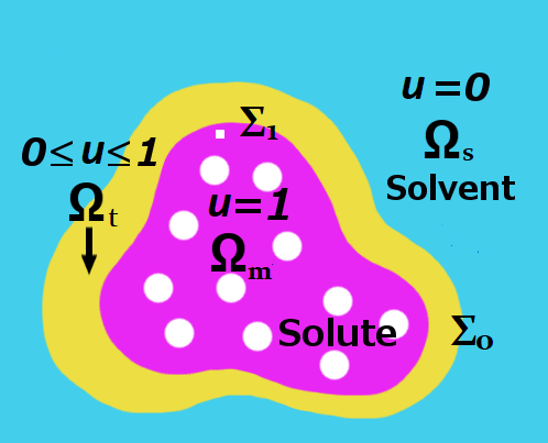
(a)

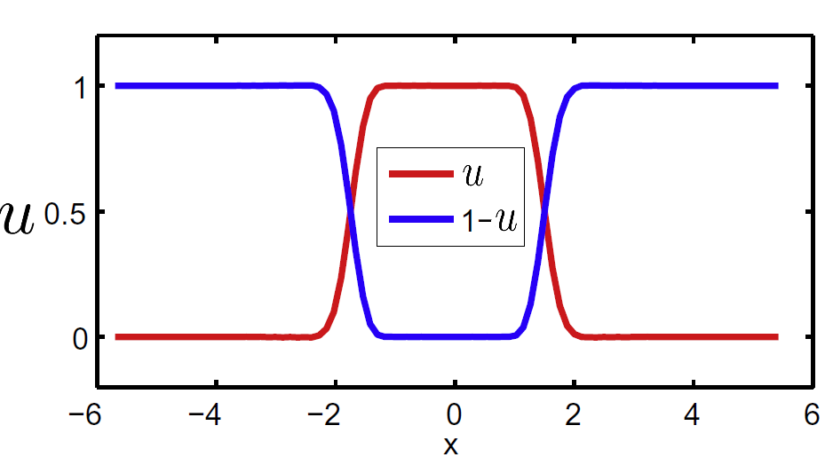
(b)

Figure 1. (A) Illustration of the model domain definition and decomposition: $\Omega_{m}$: solute (molecular) region; $\Omega_{s}$: solvent region; $\Omega_{t}$: solute-solvent mixing region; (B) The cross line of $u$ and $(1-u)$ of a diatomic system.

2.3. A Novel Solvation Energy Functional

As an improvement of the previous differential geometric based solvation model [17, 55], we study a novel solvation free energy, whose nonpolar portion is defined as

$$I_{\rm np}(u)=\gamma\int_{\Omega}d|Du|+\int_{\Omega}\left[P_{h}u^{p}+\rho_{s}(1-u^{p})U^{\mathrm{vdW}}\right]\,dx$$

with $p=\frac{2N}{2N-1}$ for some integer $N>1$ and $\lambda,P_{h}>0$. Note that $1<p<\frac{3}{2}$. Since $\frac{3}{2}=1^{*}$ is the Sobolev dual of $1$, we have

$$BV(\Omega)\hookrightarrow L^{p}(\Omega).$$

Here $u:\Omega\to\mathbb{R}$ represents a characterizing function of the solute such that $u^{p}(x)$ is the volume ratio at position $x\in\Omega$ (as shown in Figure 3). As such, the physical constraints

$$u(x)\in[0,1]\quad\text{for a.a. }x\in\Omega$$ (2.1)

and

$$u=1\quad\text{a.e. in }\Omega_{m}\quad\text{and}\quad u=0\quad\text{a.e. in }\Omega_{s}$$ (2.2)

need to be imposed. Note that $U^{\mathrm{vdW}}(x)$ can be formulated by $\sum_{i}U_{i}^{\rm att}(x)$ in which $U_{i}^{\rm att}(x)$ represents the attractive part of Lennard-Jones potential [63, 17]. To this end, the L-J potential can be divided into attractive $U_{i}^{\rm att}$ and repulsive $U_{i}^{\rm rep}$ in different ways. Here we take a Weeks-Chandler-Andersen (WCA) decomposition based on the original WCA theory [42]:

$$U_{i}^{\rm att,WCA}({\vec{r}}) = \left\{\begin{array}[]{ l l }-\epsilon_{is}(x)&0<\|x-x_{i}\|<2^{1/6}\sigma_{is}\\ U_{i}^{\rm LJ}(x){}{}{}&\|x-x_{i}\|\geq 2^{1/6}\sigma_{is},\end{array}\right.$$ (2.4)

$$U_{i}^{\rm rep,WCA}(x) = \left\{\begin{array}[]{ l l }U_{i}^{\rm LJ}(x)+\epsilon_{is}(x){}{}&0<\|x-x_{i}\|<2^{1/6}\sigma_{is}\\ 0&\|x-x_{i}\|\geq 2^{1/6}\sigma_{is}.\\ \end{array}\right.$$ (2.6)

where

$$U_{i}^{\rm LJ}(r)=4\epsilon_{is}\left[\left(\frac{\sigma_{is}}{r}\right)^{12}-\left(\frac{\sigma_{is}}{r}\right)^{6}\right]$$

with parameters $\epsilon_{is}$ of energy and $\sigma_{is}$ of length.

We choose $\Omega_{m}$ in such a way that there exist balls $B(x_{i},\tau)$ with $i=1,\cdots,N_{a}$ and $\tau>0$ such that

$$\bigcup\limits_{i=1}^{N_{a}}\overline{B}(x_{i},\tau)\subset\Omega_{m}$$ (2.7)

The polar portion of the solvation free energy is defined as

$$I_{\rm p}(u,\psi)=\int_{\Omega} \left[\rho_{m}\psi-\frac{1}{2}\epsilon(u)|\nabla\psi|^{2}-(1-u^{p})B(\psi)\right]\,dx.$$

Here $\epsilon(u)=u^{p}\epsilon_{m}+(1-u^{p})\epsilon_{s}$ is the dielectric constant of the solvent/solute mixture. $\rho_{m}$ is supported in $\Omega_{m}$. In addition, the neutral condition holds

$$\sum\limits_{j=1}^{N_{c}}c_{j}^{\infty}q_{j}=0.$$ (2.8)

Recall the definition of $B(\cdot)$ from (1.2). It is important to observe that $B(0)=0$ and, by (2.8), $B^{\prime}(0)=0$ and $B^{\prime}(\pm\infty)=\pm\infty$. Further, $B^{\prime\prime}(s)>0$. We thus conclude that $B(0)=\underset{{s\in\mathbb{R}}}{{\rm min}}B(s)$ and $B$ is strictly convex.

The problem of interest to us is to minimize the the total energy functional

$$L(u,\psi)=I_{\rm np}(u)+I_{\rm p}(u,\psi),$$ (2.9)

where $\psi$ satisfies the Dirichlet problem of a generalized Poisson-Boltzmann equation

$$\left\{\begin{aligned} {\rm div}(\epsilon(u)\nabla\psi)-(1-u^{p})B^{\prime}(\psi)&=-\rho_{m}&&\text{in}&&\Omega;\\ \psi&=\psi_{\infty}&&\text{on}&&\partial\Omega\end{aligned}\right.$$ (2.10)

for some

$$\psi_{\infty}\in W^{1,\infty}(\Omega).$$

Therefore given $u\in BV(\Omega)$ satisfying (2.1), $\psi=\psi(u)$ is determined via the elliptic boundary value problem (2.10).

With the above observations, the minimization problem can be restated as to minimize

$$I(u)=\gamma\int_{\Omega}d|Du|+\int_{\Omega}\left[P_{h}u^{p}+\rho_{s}(1-u^{p})U^{\mathrm{vdW}}\right]\,dx+\int_{\Omega}\left[\rho_{m}\psi-\frac{1}{2}\epsilon(u)|\nabla\psi|^{2}-(1-u^{p})B(\psi)\right]\,dx$$ (2.11)

in the admissible space

$$\mathcal{Y}=\{ u\in BV(\Omega):\,u\,\text{ satisfies Constraints }\eqref{constrain 1}\text{ and }\eqref{constrain 2}\}$$

and $\psi=\psi(u)$ is determined via (2.10) in the space

$$\mathcal{A}=\{v\in H^{1}(\Omega):\,v|_{\partial\Omega}=\psi_{\infty}\}.$$

3. A Family of Perturbed Poisson-Boltzmann Equation

In this section, we study a sequence of functionals associated with the polar free energy, which will be used in the numerical simulations in Section 6.

Let $\{q_{k}\}_{k=1}^{\infty}$ be a sequence of decreasing real numbers with $\lim\limits_{k\to\infty}q_{k}=1$ and taking values in $\displaystyle\left(1,\frac{\epsilon_{s}}{\epsilon_{s}-\epsilon_{m}}\right)$. In addition, set $q_{0}=1$. For any $u\in BV(\Omega)$ and $k=0,1,\cdots$, we put

$$G^{k}_{u}(\psi):=\int_{\Omega}\left[\frac{1}{2}\epsilon(u)|\nabla\psi|^{2}-\rho_{m}\psi+(q_{k}-u^{p})B(\psi)\right]\,dx.$$

Particularly, $G^{0}_{u}(\psi):=-I_{\rm p}(u,\psi)$. Further, let $\mathcal{Y}_{0}=\mathcal{Y}$ and for $k=1,2,\cdots$ define

$$\mathcal{Y}_{k}=\{u\in W^{1,q_{k}}(\Omega):\,|u|\leq\sqrt[p]{q_{k}}\text{ a.e. in }\Omega\quad\text{and $u$ satisfies Constraint~{}\eqref{constrain 2}}\}.$$ (3.1)

Correspondingly, we introduce a sequence of perturbed Poisson-Boltzmann equations for $k=0,1,\cdots$

$$\left\{\begin{aligned} {\rm div}(\epsilon(u)\nabla\psi)-(q_{k}-u^{p})B^{\prime}(\psi)&=-\rho_{m}&&\text{in}&&\Omega;\\ \psi&=\psi_{\infty}&&\text{on}&&\partial\Omega.\end{aligned}\right.$$ (3.2)

In particular, when $k=0$, (3.2) coincides with (2.10). Similar problems have been studied in [22, 44, 45, 55].

Proposition 3.1.

Given any $u\in\mathcal{Y}_{k}$, $k=0,1,\cdots$, there exists a unique $\psi_{u}\in\mathcal{A}$ such that

$$G_{u}^{k}(\psi_{u})=\underset{\psi\in\mathcal{A}}{{\rm min}}G_{u}^{k}(\psi)<\infty.$$

Moreover, $\psi_{u}$ is the unique weak solution to (3.2). Further, $\psi_{u}$ satisfies

$$\|\psi_{u}\|_{H^{1}}+\|\psi_{u}\|_{\infty}\leq\widetilde{C}_{0}.$$ (3.3)

In particular, the constant $\widetilde{C}_{0}$ is independent of $\Omega_{m}$, $\Omega_{s}$, $u$ and $k$.

Proof.

Analogous problems have been studied in the literature on various Poisson-Boltzmann type equations, cf. [22, 44, 45, 55]. In order to show the determining factors of the constant $\widetilde{C}_{0}$ in (3.3), we will, nevertheless, state a brief proof.

For every $k$, $\epsilon(u)\in L^{\infty}(\Omega)$ with $0<\epsilon_{s}-q_{1}(\epsilon_{s}-\epsilon_{m})\leq\epsilon(u)\leq\epsilon_{s}$. Standard elliptic theory, see[34, Theorems 8.3 and 8.16], implies that

$$\left\{\begin{aligned} {{\rm div}}(\epsilon(u)\nabla\psi)+\rho_{m}&=0&&\text{in}&&\Omega;\\ \psi&=\psi_{\infty}&&\text{on}&&\partial\Omega\end{aligned}\right.$$ (3.4)

has a unique weak solution $\hat{\psi}_{u}$, i.e.

$$\int_{\Omega}\epsilon(u)\nabla\hat{\psi}_{u}\cdot\nabla\phi\,dx=\int_{\Omega}\rho_{m}\phi\,dx,\quad\forall\phi\in H^{1}_{0}(\Omega),$$ (3.5)

satisfying

$$\|\hat{\psi}_{u}\|_{H^{1}}+\|\hat{\psi}_{u}\|_{\infty}\leq M_{0}.$$ (3.6)

The constant $M_{0}$ depends only on $\Omega$, $\epsilon_{s}$, $\epsilon_{m}$, $q_{1}$ and $\psi_{\infty}$. Define $\tilde{G}^{k}_{u}:H^{1}_{0}(\Omega)\to\mathbb{R}\cup\{+\infty\}$ by

$$\tilde{G}_{u}^{k}(\psi)=\int_{\Omega}\left[\frac{1}{2}\epsilon(u)|\nabla\psi|^{2}+(q_{k}-u^{p})B(\psi+\hat{\psi}_{u})\right]\,dx.$$

By the direct method of calculus of variation and the strict convexity of $\tilde{G}_{u}^{k}(\cdot)$, there exists a global minimizer $\bar{\psi}_{u}\in H^{1}_{0}(\Omega)$ of $\tilde{G}^{k}_{u}(\cdot)$. (3.5) implies

$$G_{u}^{k}(\psi)=\tilde{G}_{u}^{k}(\psi-\hat{\psi}_{u})+\int_{\Omega}\left[\frac{1}{2}\epsilon(u)|\nabla\hat{\psi}_{u}|^{2}-\rho_{m}\hat{\psi}_{u}\right]\,dx.$$

Let $\psi_{u}=\hat{\psi}_{u}+\bar{\psi}_{u}$. From the above equality, we learn that $\psi_{u}$ minimizes $G_{u}^{k}(\cdot)$ in $\mathcal{Y}_{k}$. Then following Steps (iii) and (iv) in the proof of [55, Proposition 2.2], we can show that

$$\|\bar{\psi}_{u}\|_{\infty}+\|\bar{\psi}_{u}\|_{H^{1}}\leq M_{1}$$

for some constant $M_{1}$ depending only on $M_{0}$. We can take $\widetilde{C}_{0}=M_{0}+M_{1}$. ∎

The above proposition immediately gives the following crucial estimates. For every $k$ and $u\in\mathcal{Y}_{k}$,

$$G_{u}^{k}(\psi_{u})< G_{u}^{k}(\psi_{\infty})=\int_{\Omega}\left[\frac{1}{2}\epsilon(u)|\nabla\psi_{\infty}|^{2}-\rho_{m}\psi_{\infty}+(q_{k}-u^{p})B(\psi_{\infty})\right]\,dx$$

$$\leq C\left[\|\psi_{\infty}\|_{H^{1}}^{2}+\|\psi_{\infty}\|_{\infty}+B(\|\psi_{\infty}\|_{\infty})\right]\leq\widetilde{C}_{1},$$ (3.7)

where $\psi_{u}$ is the solution to (3.2). The constant $\widetilde{C}_{1}$ is independent of $\Omega_{m}$, $\Omega_{s}$, $k$ and the choice of $u$.

Proposition 3.2.

Let $u_{k}\in\mathcal{Y}_{k}$, $k=0,1,\cdots$, be such that

$$u_{k}\to u_{0}\quad\text{in }L^{1}(\Omega)\quad\text{as }k\to\infty.$$

Let $\psi_{k}\in\mathcal{A}$ satisfy $G_{u_{k}}^{k}(\psi_{k})=\underset{w\in\mathcal{A}}{{\rm min}}G_{u_{k}}^{k}(w).$ Then

$$\psi_{k}\to\psi_{0}\quad\text{in }H^{1}(\Omega)\quad\text{and}\quad G_{u_{k}}^{k}(\psi_{k})\to G_{u_{0}}^{0}(\psi_{0})\quad\text{as }k\to\infty.$$ (3.8)

If, in addition, $u_{k}\in\mathcal{Y}$ and $\widetilde{\psi}_{k}\in\mathcal{A}$ satisfies $G_{u_{k}}^{0}(\widetilde{\psi}_{k})=\underset{w\in\mathcal{A}}{{\rm min}}G_{u_{k}}^{0}(w).$ Then

$$\widetilde{\psi}_{k}\to\psi_{0}\quad\text{in }H^{1}(\Omega)\quad\text{and}\quad G_{u_{k}}^{0}(\widetilde{\psi}_{k})\to G_{u_{0}}^{0}(\psi_{0})\quad\text{as }k\to\infty.$$ (3.9)

Proof.

We will only prove (3.8). The proof for (3.9) is similar.

Observe that since $u_{k}\to u_{0}$ in $L^{1}(\Omega)$ and $\{u_{k}\}_{k=0}^{\infty}$ are uniformly bounded in $L^{\infty}(\Omega)$. From the Riesz-Thorin interpolation theorem, we infer that $u_{k}\to u_{0}$ in $L^{r}(\Omega)$ for all $r\in[1,\infty)$. Further, by the mean value theorem

$$\lim\limits_{k\to\infty}\int|u_{k}^{p}-u_{0}^{p}|^{r}\,dx\leq M\lim\limits_{k\to\infty}\|u_{k}-u_{0}\|_{r}^{r}=0,\quad r\in[1,\infty),$$ (3.10)

for some constant $M>0$.

Due to (3.3), there exists a subsequence of $\{\psi_{k}\}_{k=1}^{\infty}$, not relabelled, and some $\psi\in H^{1}(\Omega)$ such that $\psi_{k}\to\psi$ in $L^{2}(\Omega)$ and $\psi_{k}\rightharpoonup\psi$ in $H^{1}(\Omega)$. Since $\psi_{k}$ weakly solves (3.2) with $u=u_{k}$, for any $\phi\in C^{1}_{0}(\Omega)$

$$\int_{\Omega}\left[\epsilon(u_{k})\nabla\psi_{k}\cdot\nabla\phi+(q_{k}-u_{k}^{p})B^{\prime}(\psi_{k})\phi\right]\,dx=\int_{\Omega}\rho_{m}\phi\,dx.$$ (3.11)

The dominated convergence theorem then implies that

$$\int_{\Omega}\left[\epsilon(u_{0})\nabla\psi\cdot\nabla\phi+(1-u_{0}^{p})B^{\prime}(\psi)\phi\right]\,dx=\int_{\Omega}\rho_{m}\phi\,dx.$$ (3.12)

Note that, (3.3) and a standard approximation argument imply that (3.11) and (3.12) hold for any $\phi\in H^{1}_{0}(\Omega)$. In view of Proposition 3.1, we infer that $\psi_{0}=\psi$. Next, we will show that

$$\lim\limits_{k\to\infty}\int_{\Omega}\epsilon(u_{k})|\nabla\psi_{k}-\nabla\psi_{0}|^{2}\,dx=0.$$ (3.13)

Using $\phi=\psi_{k}-\psi_{0}$ as a test function in (3.11), we conclude that

$$\lim\limits_{k\to\infty}\int_{\Omega}\epsilon(u_{k})\nabla\psi_{k}\cdot(\nabla\psi_{k}-\nabla\psi_{0})\,dx=0.$$

By the dominated convergence theorem, we have

$$\lim\limits_{k\to\infty}\int_{\Omega}\epsilon(u_{k})|\nabla\psi_{k}|^{2}\,dx=\lim\limits_{k\to\infty}\int_{\Omega}\epsilon(u_{k})\nabla\psi_{k}\cdot(\nabla\psi_{k}-\nabla\psi_{0})\,dx+\lim\limits_{k\to\infty}\int_{\Omega}\epsilon(u_{k})\nabla\psi_{k}\cdot\nabla\psi_{0}\,dx.$$

Note that $\psi=\psi_{0}-\psi_{\infty}$ weakly solves the Dirichlet problem

$$\left\{\begin{aligned} {\rm div}(\epsilon(u_{0})\nabla\psi)&=(1-u_{0}^{p})B^{\prime}(\psi_{0})-\rho_{m}-{\rm div}(\epsilon(u_{0})\nabla\psi_{\infty})&&\text{in}&&\Omega;\\ \psi&=0&&\text{on}&&\partial\Omega.\end{aligned}\right.$$

In view of (3.3), $\epsilon(u_{0})\nabla\psi_{\infty}$ and $(1-u_{0}^{p})B^{\prime}(\psi_{0})-\rho_{m}$ belong to $L^{\infty}(\Omega)$. By the Calderon-Zygmund type estimates for uniformly elliptic equation, c.f. [48, Theorem 1], there exists some $p_{0}>2$ such that $\psi_{0}\in W^{1,p_{0}}(\Omega)$. Note that [48, Theorem 1] requires $\Omega$ to be of class $\mathscr{D}^{r}$ for some $r>2$, cf. [48, Formulas (19) and (20)]. It follows from [57, Theorems B and 3.1, Lemma 4.1] (by taking $T=\nabla(-\Delta)^{-1}{\rm div}$ in [57, Theorem 3.1]) and the Poincaré’s inequality that any Lipschitz domain satisfies this condition. We thus infer from (3.10) that

$$\lim\limits_{k\to\infty}\int_{\Omega}\epsilon(u_{k})\nabla\psi_{k}\cdot\nabla\psi_{0}\,dx=\int_{\Omega}\epsilon(u_{0})|\nabla\psi_{0}|^{2}\,dx,$$ (3.14)

and in turn,

$$\lim\limits_{k\to\infty}\int_{\Omega}\epsilon(u_{k})|\nabla\psi_{k}|^{2}\,dx=\int_{\Omega}\epsilon(u_{0})|\nabla\psi_{0}|^{2}\,dx.$$ (3.15)

The dominated convergence theorem, (3.14) and (3.15) imply that

$$\lim\limits_{k\to\infty}\int_{\Omega}\epsilon(u_{k})|\nabla\psi_{k}-\nabla\psi_{0}|^{2}\,dx=\lim\limits_{k\to\infty}\int_{\Omega}\epsilon(u_{k})|\left(|\nabla\psi_{k}|^{2}-2\nabla\psi_{k}\cdot\nabla\psi_{0}+|\nabla\psi_{0}|^{2}\right)\,dx=0.$$

This establishes (3.13). It follows from the Poincaré inequality that $\psi_{k}\to\psi_{0}$ in $H^{1}(\Omega)$. The convergence $G_{u_{k}}^{k}(\psi_{k})\to G_{u_{0}}^{0}(\psi_{0})$ then can be shown by using (3.15) and the dominated convergence theorem. ∎

4. Properties of Global Minimizers

The following theorem on the existence and uniqueness of a minimizer of $I(\cdot)$ can be proved essentially in the same way as [55, Theorem 2.4] by using Propositions 3.2, A.2 and A.3.

Theorem 4.1.

There exists a unique $u_{{\rm min}}\in\mathcal{Y}$ such that $I(u_{{\rm min}})=\underset{{u\in\mathcal{Y}}}{{\rm min}}I(u)$.

To show the robustness of the model (2.11), one need to answer the question whether the solvation energy $I(u_{{\rm min}})$ depends continuously on $\Omega_{m}$ and $\Omega_{s}$ in a suitable topology? The answer to the above question is affirmative. We will present the proof of a partial result in this subsection. Due to the length of this article, a complete answer will be presented in a subsequent paper.

Assume that $\{\widetilde{\Omega}_{m;n}\}_{n=1}^{\infty}$ and $\{\widetilde{\Omega}_{s;n}\}_{n=1}^{\infty}$ are two sequences of Lipschitz subdomains such that

$$\bigcup\limits_{i}^{N_{a}}\overline{B}(x_{i},\sigma)\subset\widetilde{\Omega}_{m;n}\subseteq\Omega_{m}\quad\text{and}\quad\widetilde{\Omega}_{s;n}\subseteq\Omega_{s}\quad\text{with }\partial\Omega\subset\partial\widetilde{\Omega}_{s;n}.$$ (4.1)

We consider the sequence of energy functionals $\widetilde{I}_{n}(\cdot)$ defined by replacing $\Omega_{m}$ and $\Omega_{s}$ by $\widetilde{\Omega}_{m;n}$ and $\widetilde{\Omega}_{s;n}$ in $I(\cdot)$, respectively. The corresponding admissible spaces are

$$\widetilde{\mathcal{Y}}_{n}=\{u\in BV(\Omega):\,0\leq u\leq 1\text{ a.e. in }\Omega\quad\text{and}\quad u=1\text{ a.e. in }\widetilde{\Omega}_{m;n}\text{ and }u=0\text{ a.e. in }\widetilde{\Omega}_{s;n}\}.$$

Theorem 4.2.

Assume (4.1) and as $n\to\infty$

$$\chi_{\widetilde{\Omega}_{m;n}}\to\chi_{\Omega_{m}}\quad\text{and}\quad\chi_{\widetilde{\Omega}_{s;n}}\to\chi_{\Omega_{s}}\quad\text{in }L^{1}(\Omega).$$ (4.2)

Then for each $n$, there is a unique minimizer $u_{n}$ of $\widetilde{I}_{n}(\cdot)$ in $\widetilde{\mathcal{Y}}_{n}$. Moreover, $\lim\limits_{n\to\infty}\widetilde{I}_{n}(u_{n})=I(u_{{\rm min}})$.

Proof.

The existence and uniqueness of a minimizer of $\widetilde{I}_{n}(\cdot)$ in $\widetilde{\mathcal{Y}}_{n}$ for each $n$ follows from Theorem 4.1. Observe that $u_{{\rm min}}\in\widetilde{\mathcal{Y}}_{n}$ for all $n$. Thus

$$\widetilde{I}_{n}(u_{n})\leq I(u_{{\rm min}})=\widetilde{I}_{n}(u_{{\rm min}}).$$

This implies that

$$\gamma\int_{\Omega}d|Du_{n}|+P_{h}\|u_{n}\|_{p}^{p}+\rho_{s}\int_{\Omega\setminus\Omega_{m}}U^{\rm vdW}\,dx-\widetilde{C}_{1}\leq I(u_{{\rm min}}),$$

where $\widetilde{C}_{1}$ is the constant in (3.7). Therefore, $\|u_{n}\|_{BV}$ is uniformly bounded with respect to $n$. Proposition A.2 implies that there exists a subsequence, not relabelled, and some $u\in BV(\Omega)$ such that $u_{n}\to u$ in $L^{1}(\Omega)$. From Propositions A.3, Propositions 3.2 and the dominated convergence theorem, we infer that

$$I(u_{{\rm min}})\leq I(u)\leq\liminf\limits_{n\to\infty}\widetilde{I}_{n}(u_{n})\leq\limsup\limits_{n\to\infty}\widetilde{I}_{n}(u_{n})\leq I(u_{{\rm min}}).$$

This proves the convergence assertion. ∎

A case of particular interest is when $\Omega_{t}=\emptyset$, that is, $\Omega=\Omega_{m}\cup\Gamma\cup\Omega_{s}$ with $\Gamma=\partial\Omega_{m}\cap\partial\Omega_{s}$ being the Lipschitz sharp interface separating the solute and solvent regions. Further, suppose that $\Omega_{m}\subset\subset\Omega$. In this case, (2.11) reduces to a sharp interface model. The corresponding sharp-interface solvation free energy is given by the one proposed in [27, 28]

$$E_{0}= \gamma{\rm Per}(\Omega_{m};\Omega)+P_{h}\mathcal{L}^{3}(\Omega_{m})+\int_{\Omega_{s}}\rho_{s}U^{\mathrm{vdW}}\,dx+G_{\rm ele}(\Omega_{m}),$$ (4.3)

where ${\rm Per}(\Omega_{m};\Omega)$ is the perimeter of $\Omega_{m}$ in $\Omega$, see Appendix A, and $G_{\rm ele}(\Omega_{m})$ is the electrostatic free energy. In the classic Poisson-Boltzmann theory, it is defined by

$$G_{\rm ele}(\Omega_{m})=\int_{\Omega_{m}}\left[\rho_{m}\psi-\frac{\epsilon_{m}}{2}|\nabla\psi|^{2}\right]\,dx-\int_{\Omega_{s}}\left[\frac{\epsilon_{s}}{2}|\nabla\psi|^{2}+B(\psi)\right]\,dx,$$

cf. [2, 15, 23, 43, 56, 69, 70]. The electrostatic potential $\psi$ solves the classic sharp-interface Poisson-Boltzmann equation:

$$\left\{\begin{aligned} {\rm div}((\epsilon_{m}\chi_{\Omega_{m}}+\epsilon_{s}\chi_{\Omega_{s}})\nabla\psi)-\chi_{\Omega_{s}}B^{\prime}(\psi)&=-\rho_{m}&&\text{in}&&\Omega;\\ \psi&=\psi_{\infty}&&\text{on}&&\partial\Omega.\end{aligned}\right.$$

The following corollary shows that (4.3) is in some sense the limiting case of our diffuse interface model.

Corollary 4.3.

Assume that $\Omega=\Omega_{m}\cup\Gamma\cup\Omega_{s}$ and $\Gamma=\partial\Omega_{m}\cap\partial\Omega_{s}$ is Lipschitz. Further, suppose that $\Omega_{m}\subset\subset\Omega$. Under the same assumptions as in Theorem 4.2, $\lim\limits_{n\to\infty}\widetilde{I}_{n}(u_{n})=E_{0}.$

Remark 4.4.

In a subsequent paper, we will show that, under mild regularity assumption on $\Sigma_{1}$ and $\Sigma_{0}$, the conditions $\widetilde{\Omega}_{m;n}\subseteq\Omega_{m}$ and $\widetilde{\Omega}_{s;n}\subseteq\Omega_{s}$ in Theorem 4.2 can be relaxed.

5. How to Exclude the Formation of Sharp Interfaces?

In Theorem 4.1, we have shown that there is a unique characterizing function $u_{{\rm min}}\in BV(\Omega)$ minimizing (2.11) in $\mathcal{Y}$. However, since $BV-$functions allow jump discontinuities, a natural question to ask is whether the minimizing energy state is achieved by a sharp interface between the solute and solvent regions, or equivalently, whether the characterizing function $u_{{\rm min}}$ is the characteristic function of a set of finite perimeter.

To simplify the analysis, we will focus on the nonpolar portion of the solvation energy, i.e. (2.3). Motived by the idea in [12, 14, 13], we will show that when the mean curvature of $\Sigma_{0}$ is positive at some point, the energy minimizing state is never achieved by a sharp interface. See Theorem 5.10.

5.1. Necessary Conditions for the Minimizer of Nonpolar Energy

Throughout this section, we assume that $\Omega_{t}\neq\emptyset$. First consider the minimization problem of the nonpolar energy

$$I_{\rm np}(u)= \gamma\int_{\Omega}d|Du|+\int_{\Omega}\left[P_{h}u+\rho_{s}(1-u^{p})U^{\mathrm{vdW}}\right]\,dx$$ (5.1)

in the admissible space

$$\mathcal{X}=\{u\in BV(\Omega):\,u\,\text{ satisfies Constraint }\eqref{constrain 2}\}.$$

One will show that the minimizer $u_{{\rm min}}$ of (5.1) automatically satisfies Constraint (2.1). The reason to exclude (2.1) in the definition of the admissible space is due to the following consideration. Any subdifferential of $I_{\rm np}(\cdot)$ with Constraint (2.1) contains a function which may be discontinuous along $\partial\{u_{{\rm min}}=1\}$ and $\partial\{u_{{\rm min}}=0\}$. This will prevent us from establishing the continuity of $u_{{\rm min}}$ in these two sets.

Theorem 5.1.

(5.1) has a unique minimizer $u_{{\rm min}}\in\mathcal{X}$, which satisfies Constraint (2.1).

Proof.

Note that $\mathcal{X}$ is closed and convex in $BV(\Omega)$. Based on the strict convexity, lower semicontinuity of $I_{\rm np}$ and the direct method of Calculus of Variation, we can readily establish the existence and uniqueness of a global minimizer $u_{{\rm min}}$. If $\mathcal{L}^{3}(\{u_{{\rm min}}>1\}\cup\{u_{{\rm min}}<0\})>0$, let

$$\widetilde{u}_{\rm min}(x)=\begin{cases}1\quad&\text{when }u_{{\rm min}}(x)>1;\\ 0&\text{when }u_{{\rm min}}(x)<0;\\ u_{{\rm min}}(x)&\text{elsewhere}.\end{cases}$$

Direct computations show that $I_{\rm np}(\widetilde{u}_{\rm min})<I_{\rm np}(u_{{\rm min}})$. A contradiction. Therefore, $0\leq u_{{\rm min}}\leq 1$ a.e. in $\Omega$. ∎

Next, we derive necessary conditions for the minimizer of (5.1). We will use tools from non-smooth analysis, c.f. [29, 24, 25], to derive the subdifferential of (5.1). However, very little is known about the dual space of $BV(\Omega)$. To overcome this difficulty and tackle the Constraint (2.2), we will consider $I_{\rm np}$ as a functional defined on $L^{p}(\Omega)$ and include two extra terms. Define

$$E_{\rm np}(u)=I_{\rm np}(u)+\gamma\int_{\partial\Omega}|{\rm Tr}u|\,d\mathcal{H}^{2}+I_{K}(u)$$ (5.2)

in $L^{p}(\Omega)$, where ${\rm Tr}u$ is the trace of $u$ on $\partial\Omega$ and

$$K=\{u\in L^{p}(\Omega):\,u=1\text{ in }\Omega_{m},\text{ and }u=0\text{ in }\Omega_{s}\text{ a.e.}\}$$

and $I_{K}$ is the indicator function of $K$. In addition, we put

$$E_{1}(u)=\gamma\|Du\|(\Omega)+\gamma\int_{\partial\Omega}|{\rm Tr}u|\,d\mathcal{H}^{2},$$

and

$$E_{2}(u)=\int_{\Omega}\left[P_{h}u^{p}+\rho_{s}(1-u^{p})U^{\mathrm{vdW}}\right]\,dx.$$

The latter is Lipschitz continuous in $L^{p}(\Omega)$. It is understood that

$$E_{1}(u)=\begin{cases}\gamma\|Du\|(\Omega)+\gamma\int_{\partial\Omega}|{\rm Tr}u|\,d\mathcal{H}^{2}\quad&\text{if }u\in BV(\Omega)\\ +\infty&\text{if }u\in L^{p}(\Omega)\setminus BV(\Omega).\end{cases}$$

So, ${\rm dom}(E_{1})=BV(\Omega)$ and ${\rm dom}(I_{K})=K$. Using these notations, we can restate Problem (5.2) as to minimize a functional $E_{\rm np}:L^{p}(\Omega)\to\mathbb{R}\cup\{\infty\}$ defined by

$$E_{\rm np}(u):=E_{1}(u)+E_{2}(u)+I_{K}(u).$$ (5.3)

Direct computations show that $u_{{\rm min}}$ minimizes (5.1) in $\mathcal{X}$ iff it minimizes $E_{\rm np}(\cdot)$ in $L^{p}(\Omega)$.

Note that $K$ is closed and convex in $L^{p}(\Omega)$. This implies that $I_{K}$ is convex and lower semicontinuous. What is more, by the definition of subdifferentials, for every $u\in K$, $u^{*}\in\partial I_{K}(u)$ iff

$$\langle u^{*},u\rangle\geq\langle u^{*},v\rangle,\quad\forall v\in K.$$

Here $\langle\cdot,\cdot\rangle$ is the duality pairing between $L^{p}(\Omega)$ and $L^{p^{\prime}}(\Omega)$, that is

$$\langle v,w\rangle=\int_{\Omega}vw\,dx,\quad v\in L^{p}(\Omega),\,w\in L^{p^{\prime}}(\Omega).$$

If $\mathcal{L}^{3}(\{u^{*}>0\}\cap\Omega_{t})>0$, set $D=\{u^{*}>0\}\cap\Omega_{t}$. We define

$$v(x)=\begin{cases}u(x)+1,\quad&x\in D\\ u(x),&\text{elsewhere}.\end{cases}$$

Then $v\in K$ and

$$\langle u^{*},v-u\rangle>0.$$

A contradiction. Similarly, we can show that $\mathcal{L}^{3}(\{u^{*}<0\}\cap\Omega_{t})=0$. Thus, $u^{*}=0$ a.e. in $\Omega_{t}$. This is also the sufficient condition of $u^{*}\in\partial I_{K}(u)$. Indeed, given any $u^{*}\in L^{p^{\prime}}(\Omega)$ with $u^{*}=0$ a.e. in $\Omega_{t}$, for any $v\in K$,

$$\langle u^{*},v-u\rangle=\int_{\Omega\setminus\Omega_{t}}u^{*}(u-v)\,dx+\int_{\Omega_{t}}u^{*}(u-v)\,dx=0.$$

To sum up, a function $u^{*}\in L^{p^{\prime}}(\Omega)$ belongs to $\partial I_{K}(u)$ iff $u^{*}=0$ in $\Omega_{t}$.

To compute $\partial E_{1}(u)$, we define

$$X^{\infty}_{p^{\prime}}:=\{z\in L^{\infty}(\Omega,\mathbb{R}^{3}):\,{\rm div}z\in L^{p^{\prime}}(\Omega)\}.$$

Here, ${\rm div}z\in L^{p^{\prime}}(\Omega)$ means that there exists $f\in L^{p^{\prime}}(\Omega)$ such that

$$\int_{\Omega}f\phi\,dx=-\int_{\Omega}z\cdot\nabla\phi\,dx$$

for all $\phi\in C_{0}^{\infty}(\Omega)$. Given any $u\in BV(\Omega)$ and $z\in X^{\infty}_{p^{\prime}}$, there exists a Radon measure, denoted by $z\cdot Du$, such that for any $\phi\in C_{0}^{\infty}(\Omega)$, with a little abuse of notation,

$$\langle z\cdot Du,\phi\rangle:=\int_{\Omega}\phi(z\cdot Du)=-\int_{\Omega}uz{\rm div}\phi\,dx-\int_{\Omega}u\phi{\rm div}z\,dx.$$

The measure $z\cdot Du$ is absolutely continuous with respect to $|Du|$. By the Radon-Nikodym Theorem, there is a $|Du|$-measurable function $\theta(z,Du)$ s.t.

$$\int_{A}z\cdot Du=\int_{A}\theta(z,Du)d|Du|$$ (5.4)

for all Borel sets $A\subseteq\Omega$. Let

$$M^{*}_{p^{\prime}}:=\{v^{*}\in L^{p^{\prime}}(\Omega):\,v^{*}=-{\rm div}z\text{ for some }z\in X^{\infty}_{p^{\prime}}\text{ with }\|z\|_{\infty}\leq 1\}.$$

One can follow the idea of [39, Proposition 4.23(1)] and prove that

$$u^{*}\in\partial E_{1}(u)\quad\text{iff}\quad E_{1}(u)=\gamma\langle u^{*},u\rangle,\quad u^{*}\in M^{*}_{p^{\prime}},$$

that is,

$$E_{1}(u)=-\gamma\int_{\Omega}u{\rm div}z\,dx=\gamma\int_{\Omega}z\cdot Du-\gamma\int_{\partial\Omega}(z\cdot\nu_{\partial\Omega})u\,d\mathcal{H}^{2}$$ (5.5)

for some $z\in X^{\infty}_{p^{\prime}}$ with $\|z\|_{\infty}\leq 1$, where $\nu_{\partial\Omega}$ is the outward unit normal of $\Omega$. The last equality follows from [3, Theorem 1.9]. In addition, [3, Corollary 1.6] shows that $\|z\|_{\infty}=1$ whenever $u\neq 0$.

Next, Proposition B.1 implies that for any $u\in L^{p}(\Omega)$,

$$\partial E_{2}(u)=pP_{h}u^{p-1}-p\rho_{s}u^{p-1}U^{\rm vdW}.$$

Because of the lack of continuity of $E_{1}$ and $I_{K}$, in general, we can only conclude that $\partial E_{1}(u)+\partial I_{K}(u)\subseteq\partial(E_{1}+I_{K})(u)$. In order to compute $\partial(E_{1}+I_{K})(u)$, we will use Propositions B.3. It suffices to verify the closed linear space condition. An easy computation shows that

$${\rm dom}(E_{1})-{\rm dom}(I_{K})=\{v\in L^{p}(\Omega):\,v|_{\Omega_{m}\cup\Omega_{s}}\in BV(\Omega_{m}\cup\Omega_{s})\},$$

which is obviously a linear subspace of $L^{p}(\Omega)$. We learn from Propositions A.3 and A.6 that ${\rm dom}(E_{1})-{\rm dom}(I_{K})$ is closed. Now Proposition B.3 immediately implies that

$$\partial(E_{1}+I_{K})(u)=\partial E_{1}(u)+\partial I_{K}(u).$$

We thus have

$$\partial E(u)=\partial E_{1}(u)+\partial E_{2}(u)+\partial I_{K}(u).$$ (5.6)

From the definition of subdifferential and (5.6), we learn that

$$u\in\mathcal{X}\text{ minimizes }\eqref{minimization pb nonpolar 2}\quad\text{iff}\quad 0\in\partial E(u)=\partial E_{1}(u)+\partial E_{2}(u)+\partial I_{K}(u).$$

More precisely, this means that there is some $z\in X^{\infty}_{p^{\prime}}$ with $\|z\|_{\infty}=1$ satisfying (5.5) and $w\in L^{p^{\prime}}(\Omega)$ with $w\equiv 0$ in $\Omega_{t}$ such that

$$0=-\gamma{\rm div}z+pu_{{\rm min}}^{p-1}\left(P_{h}-\rho_{s}U^{\mathrm{vdW}}\right)+w\quad\text{in }\Omega,$$ (5.7)

where $z$ satisfies

$$\int_{\Omega}z\cdot Du_{{\rm min}}=-\int_{\Omega}u_{{\rm min}}{\rm div}z\,dx=\|Du_{{\rm min}}\|(\Omega).$$

In particular, it holds that

$$0=-\gamma{\rm div}z+pu_{{\rm min}}^{p-1}\left(P_{h}-\rho_{s}U^{\mathrm{vdW}}\right)\quad\text{in }\Omega_{t}.$$

5.2. Regularity of the Minimizer $u_{{\rm min}}$

As in the previous subsection, $u_{{\rm min}}$ is the minimizer of (5.2) in $L^{p}(\Omega)$. Set

$$E_{t}:=\{u_{{\rm min}}>t\},\quad t\in[0,1)$$ (5.8)

to be the super-level sets of $u_{{\rm min}}$. Recall $\Omega_{w}=\Omega\setminus\overline{\Omega}_{s}$.

Proposition 5.2.

For all $t\in[0,1)$, $E_{t}$ is a solution of

$$\underset{E\in\mathcal{M}}{{\rm min}}\left[\gamma{\rm Per}(E;\Omega)+\int_{E}pt^{p-1}\left(P_{h}-\rho_{s}U^{\mathrm{vdW}}\right)\,dx\right],$$ (5.9)

where the minimum is taken in the set

$$\mathcal{M}=\{E\subset\Omega\text{ is of finite perimeter}:\,\Omega_{m}\subseteq E\subseteq\Omega_{w}\}.$$

Proof.

Take $z$ as in (5.7). (5.4) and (5.5) show that

$$\|Du_{{\rm min}}\|(\Omega)=\int_{\Omega}z\cdot Du_{{\rm min}}=\int_{\Omega}\theta(z,Du_{{\rm min}})d|Du_{{\rm min}}|.$$

By [3, Corollary 1.6], it holds that $\|\theta(z,Du_{{\rm min}})\|_{L^{\infty}(\Omega,|Du_{{\rm min}}|)}\leq\|z\|_{\infty}=1$. We thus infer that $\theta(z,Du_{{\rm min}})=1$ $|Du_{{\rm min}}|$-a.e. For any $a,b\in[0,1)$ with $a<b$, define

$$v(x)=\begin{cases}b\quad&\text{if }u_{{\rm min}}(x)>b\\ u_{{\rm min}}(x)&\text{if }a\leq u_{{\rm min}}(x)\leq b\\ a&\text{if }u_{{\rm min}}(x)<a.\end{cases}$$

Given any $\phi\in C_{0}(\Omega)$, by [3, Proposition 2.7(i) and Formula (2.15)], we have

$$\int_{\Omega}\phi\,d|Dv|=\int_{\Omega}\phi\theta(z,Dv)d|Dv|=\langle z\cdot Dv,\phi\rangle=\int_{a}^{b}\int_{\Omega}\phi(z\cdot D\chi_{E_{t}})\,dt.$$

On the other hand, by the coarea formula (A.4),

$$\int_{\Omega}\phi\,d|Dv|=\int_{a}^{b}\int_{\Omega}\phi\,d|D\chi_{E_{t}}|\,dt.$$

It shows that

$$\int_{a}^{b}\int_{\Omega}\phi(z\cdot D\chi_{E_{t}})\,dt=\int_{a}^{b}\int_{\Omega}\phi\,d|D\chi_{E_{t}}|\,dt,\quad\forall\phi\in C^{\infty}_{0}(\Omega).$$

Because $a$ and $b$ are arbitrary, $(z\cdot D\chi_{E_{t}})=|D\chi_{E_{t}}|$ in the sense of measure for a.a. $t\in[0,1)$. This implies that

$$\int_{\Omega}z\cdot D\chi_{E_{t}}=\|D\chi_{E_{t}}\|(\Omega)\quad\text{for a.a. }t\in[0,1).$$ (5.10)

Denote by $D$ the set of all $t$ satisfying (5.10). If $t\in D$, (5.10) and [3, Corollary 1.6, Theorem 1.9] imply that

$$-\int_{\Omega}{\rm div}z(\chi_{F}-\chi_{E_{t}})\,dx= \int_{\Omega}z\cdot D\chi_{F}\,dx-\int_{\Omega}z\cdot D\chi_{E_{t}}\,dx=\int_{\Omega}z\cdot D\chi_{F}\,dx-{\rm Per}(E_{t};\Omega)$$

$$\leq {\rm Per}(F;\Omega)-{\rm Per}(E_{t};\Omega)$$

holds for all $F\in\mathcal{M}$. Combining with (5.7), we thus deduce that

$$\gamma{\rm Per}(F;\Omega)-\gamma{\rm Per}(E_{t};\Omega)$$

$$\geq -\int_{\Omega}pu_{{\rm min}}^{p-1}\left(P_{h}-\rho_{s}U^{\mathrm{vdW}}\right)(\chi_{F}-\chi_{E_{t}})\,dx-\int_{\Omega}w(\chi_{F}-\chi_{E_{t}})\,dx$$

$$\geq -\int_{\Omega}pt^{p-1}\left(P_{h}-\rho_{s}U^{\mathrm{vdW}}\right)(\chi_{F}-\chi_{E_{t}})\,dx$$

$$+\int_{\Omega}p(t^{p-1}-u_{{\rm min}}^{p-1})\left(P_{h}-\rho_{s}U^{\mathrm{vdW}}\right)(\chi_{F}-\chi_{E_{t}})\,dx$$

$$\geq -\int_{\Omega}pt^{p-1}\left(P_{h}-\rho_{s}U^{\mathrm{vdW}}\right)(\chi_{F}-\chi_{E_{t}})\,dx$$

by observing that

$$(t^{p-1}-u_{{\rm min}}^{p-1})(P_{h}-\rho_{s}U^{\mathrm{vdW}})(\chi_{F}-\chi_{E_{t}})\geq 0$$

and

$$\int_{\Omega}w(\chi_{F}-\chi_{E_{t}})\,dx=0.$$

If $t\notin D$, then take a decreasing sequence $\{t_{n}\}_{n=1}^{\infty}\subset D$ such that $t_{n}\to t^{+}$. It is clear that $\bigcup\limits_{n}E_{t_{n}}=E_{t}$. By the dominated convergence theorem, $\chi_{E_{t_{n}}}\to\chi_{E_{t}}$ in $L^{1}(\Omega)$. Then Proposition A.3 shows that

$${\rm Per}(E_{t};\Omega)\leq\liminf\limits_{n\to\infty}{\rm Per}(E_{t_{n}};\Omega).$$

On the other hand, (5.10) and [3, Corollary 1.6 and Theorem 1.9] imply that

$${\rm Per}(E_{t_{n}};\Omega) =\int_{\Omega}z\cdot D\chi_{E_{t_{n}}}=-\int_{E_{t_{n}}}{\rm div}z\,dx$$

$$\to -\int_{E_{t}}{\rm div}z\,dx=\int_{\Omega}z\cdot D\chi_{E_{t}}\leq{\rm Per}(E_{t};\Omega),\quad\text{as }n\to\infty.$$

Therefore, (5.10) holds for $t$. We thus deduce that the assertion holds for any $t\in[0,1)$. ∎

Remark 5.3.

The existence of a minimizer of (5.9) can be proved by using the classical method of Calculus of Variation for every $t\in[0,1)$. See [38] for a related problem.

Lemma 5.4.

Let $t^{\prime}<t$. If $F_{t}$ and $F_{t^{\prime}}$ are minimizers of (5.9) with $t$ and $t^{\prime}$, respectively, then $F_{t}\subseteq F_{t^{\prime}}$.

Proof.

We clearly have

$$\gamma{\rm Per}(F_{t};\Omega)+\int_{F_{t}}pt^{p-1}\left(P_{h}-\rho_{s}U^{\mathrm{vdW}}\right)\,dx\leq\gamma{\rm Per}(F_{t}\cap U_{t^{\prime}};\Omega)+\int_{F_{t}\cap F_{t^{\prime}}}pt^{p-1}\left(P_{h}-\rho_{s}U^{\mathrm{vdW}}\right)\,dx$$

and

$$\gamma{\rm Per}(F_{t^{\prime}};\Omega)+\int_{F_{t^{\prime}}}p({t^{\prime}})^{p-1}\left(P_{h}-\rho_{s}U^{\mathrm{vdW}}\right)\,dx\leq\gamma{\rm Per}(F_{t}\cup F_{t^{\prime}};\Omega)+\int_{F_{t}\cup F_{t^{\prime}}}p({t^{\prime}})^{p-1}\left(P_{h}-\rho_{s}U^{\mathrm{vdW}}\right)\,dx.$$

Because

$${\rm Per}(F_{t}\cap F_{t^{\prime}};\Omega)+{\rm Per}(F_{t}\cup F_{t^{\prime}};\Omega)\leq{\rm Per}(F_{t};\Omega)+{\rm Per}(F_{t^{\prime}};\Omega),$$

we deduce that

$$({t^{\prime}})^{p-1}\left[\int_{F_{t^{\prime}}}\left(P_{h}-\rho_{s}U^{\mathrm{vdW}}\right)\,dx-\int_{F_{t}\cup F_{t^{\prime}}}\left(P_{h}-\rho_{s}U^{\mathrm{vdW}}\right)\,dx\right]$$

$$\leq t^{p-1}\left[\int_{F_{t}\cap F_{t^{\prime}}}\left(P_{h}-\rho_{s}U^{\mathrm{vdW}}\right)\,dx-\int_{F_{t}}\left(P_{h}-\rho_{s}U^{\mathrm{vdW}}\right)\,dx\right],$$

i.e.

$$({t^{\prime}})^{p-1}\int_{F_{t}\setminus F_{t^{\prime}}}\left(P_{h}-\rho_{s}U^{\mathrm{vdW}}\right)\,dx\geq t^{p-1}\int_{F_{t}\setminus F_{t^{\prime}}}\left(P_{h}-\rho_{s}U^{\mathrm{vdW}}\right)\,dx.$$

But $t^{\prime}<t$. This implies that $F_{t}\subseteq F_{t^{\prime}}$. ∎

Proposition 5.5.

For all but countably many $t\in(0,1]$, the minimizer of (5.9) is unique, i.e. $E_{t}$.

Proof.

Fix $t\in(0,1)$ and assume that $F$ is a minimizer of (5.9). Take an arbitrary increasing sequence $\{s_{n}\}_{n=1}^{\infty}\subseteq(0,1)$ and an arbitrary decreasing sequence $\{t_{n}\}_{n=1}^{\infty}\subseteq(0,1)$ such that $\lim\limits_{n\to\infty}s_{n}=t=\lim\limits_{n\to\infty}t_{n}$.

It follows from Proposition 5.2 and Lemma 5.4 that

$$\bigcup\limits_{n}E_{t_{n}}\subseteq F\subseteq\bigcap\limits_{n}E_{s_{n}}.$$

Note that

$$\bigcap\limits_{n}E_{s_{n}}=E_{t}\cup\{u=t\}\quad\text{and}\quad\bigcup\limits_{n}E_{t_{n}}=E_{t}.$$

However, there are only countably many $t$ such that $\mathcal{L}^{3}(\{u=t\})>0$. This implies that

$$F=E_{t}\quad\text{for a.a. }t\in[0,1).$$

This completes the proof. ∎

Proposition 5.6.

For any $t\in[0,1)$, the singular set of $E_{t}$ is contained in $\Sigma_{0}\cup\Sigma_{1}$ and $\partial E_{t}\setminus(\Sigma_{0}\cup\Sigma_{1})$ is of class $C^{\infty}$.

Proof.

For any $x\in\partial E_{t}\cap\Omega_{t}$, for sufficiently small $r>0$, the ball $B(x,r)$ is contained in $\Omega_{t}$. For any local perturbation of $E_{t}$ in $B(x,r)$, i.e. a set $F$ of finite perimeter such that $F\Delta E_{t}=(F\setminus E_{t})\cup(E_{t}\setminus F)\subset\!\subset B(x,r)$, we have

$${\rm Per}(E_{t};B(x,r))\leq {\rm Per}(F;B(x,r))+C\int_{B(x,r)}pt^{p-1}\left(P_{h}-\rho_{s}U^{\mathrm{vdW}}\right)\,dx$$

$$\leq {\rm Per}(F;B(x,r))+Cr^{2+\delta}$$

by Hölder inequality for any $\delta\in(0,1)$. Note that the constant $C$ in the above inequality is independent of the position of $x$. Hence $E_{t}\cap\Omega_{t}$ is almost minimal in $\Omega_{t}$ in the sense of [60, Definition 1.5]. Therefore, [60, Theorem 1.9] implies that the singular set of $E_{t}$ is contained in $\Sigma_{0}\cup\Sigma_{1}$ and $\partial E_{t}\setminus(\Sigma_{0}\cup\Sigma_{1})$ is a $C^{1}$-hypersurface. Then the assertion follows from the standard regularity theorem of non-parametric minimizing surfaces, see [35] for example. For the reader’s convenience, we will state a proof here. For every $x_{0}\in\partial E_{t}\setminus(\Sigma_{0}\cup\Sigma_{1})$, denote by $H_{x_{0}}$ the tangent plane of $\partial E_{t}$ at $x_{0}$. Near $x_{0}$, we can rewrite the coordinates in the form $x=(y,z)$, where $y$ is the coordinates in $H$ and $z$ is the coordinate in the normal direction of $H$. We use the convention $z=y=0$ at $x_{0}$. For sufficiently small $r>0$, let $U_{r}=B(x,r)\cap H_{x_{0}}$. Build a cylinder $C_{r}=U_{r}\times(-r,r)\subset\subset\Omega_{t}$ in $(y,z)-$coordinates centered at $x_{0}$. Inside $C_{r}$, we can express $\partial E_{t}$ as the graph of a $C^{1}-$function $v$:

$$z=v(y),\quad y\in U_{r}.$$

See Figure 2.

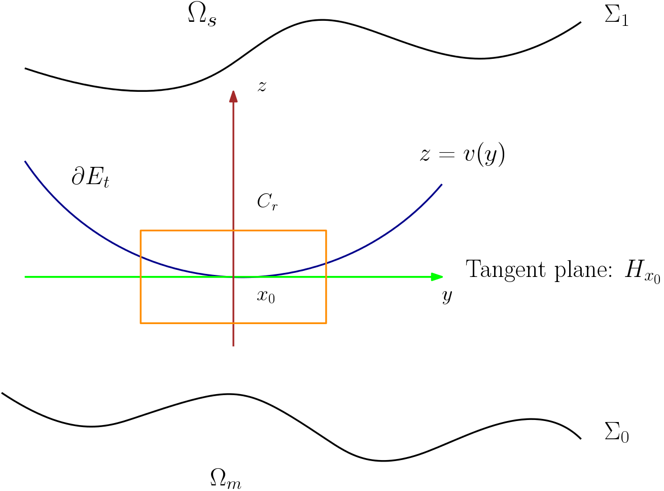
Figure 2. A coordinate system near $x_{0}\in\partial E_{t}\setminus(\Sigma_{0}\cup\Sigma_{1})$

Then

$$\gamma{\rm Per}(E_{t};C_{r})+\int_{C_{r}\cap E_{t}}pt^{p-1}\left(P_{h}-\rho_{s}U^{\mathrm{vdW}}\right)\,dx$$

$$= \gamma\int_{U_{r}}\sqrt{1+|\nabla_{y}v(y)|^{2}}\,dy+\int_{U_{r}}\int_{0}^{v(y)}\left(P_{h}-\rho_{s}U^{\mathrm{vdW}}(y,z)\right)\,dzdy.$$

By the fundamental theorem of Calculus, $v$ solves

$$\left\{\begin{aligned} A(v)v&=f(y,v(y))&&\text{in}&&U_{r};\\ v&=g&&\text{on}&&\partial U_{r}\end{aligned}\right.$$

for some $g\in C^{1}(\partial U_{r})$. Here

$$A(v)w=\frac{\Delta_{y}w(y)}{\sqrt{1+|\nabla_{y}v(y)|^{2}}}-\frac{(\nabla_{y}v)\nabla^{2}_{y}w(\nabla_{y}v)^{T}}{(\sqrt{1+|\nabla_{y}v(y)|^{2}})^{3}},\quad f(y,z)=\left(P_{h}-\rho_{s}U^{\mathrm{vdW}}(y,z)\right)/\gamma.$$

By choosing $r>0$ sufficiently small, one can infer from [34, Theorems 16.10] that $v\in C^{2}(\overline{U_{r}})$. The remaining regularity follows from a bootstrapping argument, cf. [34, Theorems 6.13 and 6.17]. ∎

Remark 5.7.

If we assume, in addition, that $\Sigma_{i}\in C^{1,1}$ for $i=0,1$, then following the argument in [60, Section 1.14(iv)], one can show that the singular set of $E_{t}$ is empty and $\partial E_{t}\in C^{1,1}$. Since this fact will not be used below, to keep the article in a reasonable length, we will not provide a rigorous proof here.

Proposition 5.8.

The jump set, $J_{u_{{\rm min}}}$, of $u_{{\rm min}}$ is contained in $\Sigma_{0}\cup\Sigma_{1}$.

Proof.

The proof follows the idea in [13, Theorem 3.4]. By (A.5), it suffices to show that for any $t_{1}<t_{2}\in[0,1)$ and $t_{1},t_{2}\in\mathbb{Q}$, it holds

$$(\partial E_{t_{1}}\cap\partial E_{t_{2}})\setminus(\Sigma_{0}\cup\Sigma_{1})=\emptyset.$$

Assume that $x_{0}\in(\partial E_{t_{1}}\cap\partial E_{t_{2}})\setminus(\Sigma_{0}\cup\Sigma_{1})$. By Proposition 5.6, both $\partial E_{t_{1}}$ and $\partial E_{t_{2}}$ are regular in a neighbourhood of $x_{0}$. From the fact $E_{t_{2}}\subseteq E_{t_{1}}$, we deduce that the tangent space of $E_{t_{2}}$ and $E_{t_{1}}$ at $x_{0}$ agree. Denote the tangent space by $H_{x_{0}}$. We define the coordinates in the form $x=(y,z)$ and the cylinder $C_{r}=(-r,r)\times U_{r}$ as in the previous proof. Then we can express $E_{t_{i}}$ with $i=1,2$ as graphs over $U_{r}$ as

$$z=v_{i}(y)\quad i=1,2$$

with $v_{i}\in C^{\infty}(U_{r})$. $E_{t_{2}}\subseteq E_{t_{1}}$ implies that $v_{1}\geq v_{2}$ in $U_{r}$. Similar to the previous proof, we have

$$\gamma{{\rm div}}_{y}\left(\frac{\nabla_{y}v_{i}(y)}{\sqrt{1+|\nabla_{y}v_{i}(y)|^{2}}}\right)=pt_{i}^{p-1}\left(P_{h}-\rho_{s}U^{\mathrm{vdW}}(y,v_{i}(y))\right).$$

Since $t_{2}>t_{1}$, $v_{i}(0)=0$, $\nabla_{y}v_{i}(0)=0$, by choosing $r>0$ small enough, we have

$$pt_{2}^{p-1}\left(P_{h}-\rho_{s}U^{\mathrm{vdW}}(y,v_{2}(y))\right)\Big{(}\sqrt{1+|\nabla_{y}v_{2}(y)|^{2}}\Big{)}^{3}>pt_{1}^{p-1}\left(P_{h}-\rho_{s}U^{\mathrm{vdW}}(y,v_{1}(y))\right)\Big{(}\sqrt{1+|\nabla_{y}v_{1}(y)|^{2}}\Big{)}^{3}$$

for all $y\in U_{r}$. This implies that

$$\left(1+|\nabla_{y}v_{2}|^{2}\right)\Delta_{y}v_{2}-\nabla_{y}v_{2}\nabla^{2}_{y}v_{2}\nabla_{y}v_{2}>\left(1+|\nabla_{y}v_{1}|^{2}\right)\Delta_{y}v_{1}-\nabla_{y}v_{1}\nabla^{2}_{y}v_{1}\nabla_{y}v_{1}$$

in $U_{r}$. In view of the boundary condition $v_{1}\geq v_{2}$ on $\partial U_{r}$, we infer from [34, Theorem 10.1] that $v_{2}<v_{1}$ in $U_{r}$, which contradicts $v_{1}(x_{0})=v_{2}(x_{0})$. Therefore, $(\partial E_{t_{1}}\cap\partial E_{t_{2}})\setminus(\Sigma_{0}\cup\Sigma_{1})=\emptyset$. ∎

Remark 5.9.

In particular, Proposition 5.8 implies that $u\in C(\Omega_{t})$.

5.3. Necessary Conditions for the Formation of a Sharp Interface

In this section, we first consider the case that $\Omega_{t}$ is connected. In order to state the main theorem of this section, we define the orientations of $\Sigma_{i}$ in such a way that

• the outer normal of $\Sigma_{1}$ points into $\Omega_{t}$, and

• the outer normal of $\Sigma_{0}$ points into $\Omega_{s}$.

With these conventions, a sphere of radius $R>0$ has constant mean curvature $-1/R$.

Theorem 5.10.

Suppose that $\Omega_{t}$ is connected and $\Sigma_{i}$, for $i=0,1$, are $C^{2}-$closed surfaces. Let $\kappa$ be the mean curvature of $\Sigma_{1}$. If $\kappa(\mathsf{p})>0$ for some $\mathsf{p}\in\Sigma_{1}$, then there is no sharp solute-solvent interface, that is, the minimizer $u_{{\rm min}}$ of (2.11) is not the characteristic function of a set $E$ of finite perimeter with $\Omega_{m}\subseteq E\subseteq\Omega_{w}$.

Proof.

Assume, to the contrary, that there exists a set $E$ of finite perimeter such that $\Omega_{m}\subseteq E\subseteq\Omega_{w}$ and $\chi_{E}$ minimizes (2.11).

(1) By the De Giorgi Theorem, cf. [1, Theorem 3.59 and Example 3.68], we have

$$\partial^{*}E\subseteq J_{\chi_{E}}\subseteq\Sigma_{0}\cup\Sigma_{1}.$$

For every $x\in\Omega_{t}\cap E$, (A.2) implies that ${\rm Per}(E;B(x,r))=0$ for all $r>0$ so small that $B(x,r)\subset\Omega_{t}$. Thus the isoperimeteric inequality, cf. [30, Theorem 5.6.2], implies that

$${\rm min}\{\mathcal{L}^{3}(B(x,r)\cap E),\mathcal{L}^{3}(B(x,r)\setminus E)\}^{2/3}\leq C{\rm Per}(E;B(x,r))=0.$$

If $\mathcal{L}^{3}(E\cap\Omega_{t})>0$, assume that there exist two distinct points $x_{1},x_{2}\in\Omega_{t}$ such that $\mathcal{L}^{3}(B(x_{1},r)\cap E)=0$ and $\mathcal{L}^{3}(B(x_{2},r)\setminus E)=0$. Since $\Omega_{t}$ is connected, we can find a continuous path $\gamma:[0,1]\to\Omega_{t}$ such that

$$\gamma(0)=x_{1},\quad\gamma(1)=x_{2}.$$

Further assume that $r>0$ is so small that $B(x,r)\subset\Omega_{t}$ for all $x\in\gamma([0,1]).$ Then for any $x\in\gamma([0,1])\cap B(x_{1},r)$, we have $\mathcal{L}^{3}(B(x,r)\cap E)=0$. Repeating this argument for finitely many times shows that $\mathcal{L}^{3}(B(x_{2},r)\cap E)=0$. A contradiction. Therefore, $\mathcal{L}^{3}(B(x,r)\setminus E)=0$ for all $x\in\Omega_{t}$ and all $r>0$ so small that $B(x,r)\subset\Omega_{t}$. We immediately infer that

$$\mathcal{L}^{3}(\Omega_{t}\setminus E)=0$$

and thus $\chi_{E}=\chi_{\Omega_{w}}$ a.e. To sum up, we have either $E=\Omega_{m}$ or $E=\Omega_{w}$.

(2) Consider the case that $E=\Omega_{m}$, or equivalently $u_{{\rm min}}=\chi_{E}$. Define $E_{t}$ as in (5.8). Then for each $t\in[0,1)$, $E_{t}=\Omega_{m}$. Therefore, $\chi_{\Omega_{m}}$ is the unique minimizer of (5.9) for every $t\in[0,1)$.

Since $\Sigma_{1}$ is $C^{2}$, it has a tubular neighborhood $B_{\mathfrak{a}}(\Sigma_{1})$ of width $\mathfrak{a}>0$, cf. [34, Exercise 2.11] and [41, Remark 3.1]. Given any $\rho\in C^{1}(\Sigma_{1})$ with $0\leq\rho\leq 1$, the map

$$\Psi_{\rho}:(-\mathfrak{a},\mathfrak{a})\times\Sigma_{1}\to\mathbb{R}^{3}:\,(\varepsilon,\mathsf{p})\mapsto\mathsf{p}+\varepsilon\rho(\mathsf{p})\nu_{\Sigma_{1}}(\mathsf{p}),$$

is a $C^{1}$-diffeomorphism onto its image, where $\nu_{\Sigma_{1}}$ is the outward unit normal of $\Sigma_{1}$ pointing into $\Omega_{t}$. Put $\Gamma_{\varepsilon}:=\Psi_{\rho}(\varepsilon,\Sigma)$ and $\Omega_{\varepsilon}$ as the region enclosed by $\Gamma_{\varepsilon}$. Observe that $\Omega_{0}=\Omega_{m}$ and

$$\Omega_{m}\subseteq\Omega_{\varepsilon}\subseteq\Omega_{w}$$

for all $\varepsilon\in[0,\mathfrak{a})$ with sufficiently small $\mathfrak{a}$. Define a functional

$$F_{t}(\varepsilon)=\gamma{\rm Per}(\Gamma_{\varepsilon};\Omega)+\int_{\Omega_{\varepsilon}}pt^{p-1}\left(P_{h}-\rho_{s}U^{\mathrm{vdW}}\right)\,dx,\quad\varepsilon\in[0,\mathfrak{a}).$$

Note that $F_{t}(\varepsilon)\geq F_{t}(0)$. By [38, Equation (21)],

$$\lim\limits_{\varepsilon\to 0^{+}}\frac{F_{t}(\varepsilon)-F_{t}(0)}{\varepsilon}= \int_{\Sigma_{1}}\rho\left(-2\gamma\kappa+pt^{p-1}P_{h}-pt^{p-1}\rho_{s}U^{\mathrm{vdW}}\right)\,d\Sigma_{1},$$

where $d\Sigma_{1}$ is the volume element on $\Sigma_{1}$. Thus

$$\int_{\Sigma_{1}}\rho\left(-2\gamma\kappa+pt^{p-1}P_{h}-pt^{p-1}\rho_{s}U^{\mathrm{vdW}}\right)\,d\Sigma_{1}\geq 0$$

for all $\rho\in C^{1}(\Sigma_{1})$ with $\rho\geq 0$. This implies that

$$pt^{p-1}P_{h}-pt^{p-1}\rho_{s}U^{\mathrm{vdW}}\geq 2\gamma\kappa$$

for all $t\in[0,1)$. Taking $t=0$ above yields

$$0\geq\kappa\quad\text{on }\Sigma_{1}.$$

This is a necessary condition for $E=\Omega_{m}$. Therefore, if $\kappa(\mathsf{p})>0$ for some $\mathsf{p}\in\Sigma_{1}$, then $E\neq\Omega_{m}$.

(3) Let $\widehat{\kappa}$ be the mean curvature of $\Sigma_{0}$. If $E=\Omega_{w}$, then following the above argument, we conclude that

$$\int_{\Sigma_{0}}\rho\left(-2\gamma\widehat{\kappa}+pt^{p-1}P_{h}-pt^{p-1}\rho_{s}U^{\mathrm{vdW}}\right)\,d\Sigma_{0}\geq 0$$

for all $\rho\in C^{1}(\Sigma_{0})$ with $\rho\leq 0$ and $t\in[0,1)$. Here $d\Sigma_{0}$ is the volume element on $\Sigma_{0}$. Pushing $t\to 1^{-}$ implies that

$$\widehat{\kappa}\geq\frac{pP_{h}-p\rho_{s}U^{\mathrm{vdW}}}{2\gamma}>0$$

is a necessary condition for $E=\Omega_{w}$ However, it is well known that there is no closed hypersurface with everywhere positive mean curvature in $\mathbb{R}^{3}$. Therefore, $E\neq\Omega_{w}$ ∎

Remark 5.11.

The mean curvature condition $\kappa(\mathsf{p})>0$ for some $\mathsf{p}\in\Sigma_{1}$ is satisfied by almost all macromolecules. This explains why diffuse interfaces are indeed more realistic in real-world solvation processes. It is equally important to point out that the mean curvature condition is in some sense “stable”. Recall that the Hausdorff metric on compact subsets $K\subset\mathbb{R}^{n}$, $n\in\mathbb{N}$, is defined by

$$d_{\mathcal{H}}(K_{1},K_{2})={\rm max}\left\{\sup\limits_{x\in K_{1}}d(x,K_{2}),\sup\limits_{x\in K_{2}}d(x,K_{1})\right\}.$$

Given a closed surface $\Sigma$ in $\mathbb{R}^{3}$, its second normal bundle is given by

$$\mathcal{N}^{2}\Sigma=\{(\mathsf{p},\nu_{\Sigma}(\mathsf{p}),\nabla_{\Sigma}\nu_{\Sigma}(\mathsf{p})):\,\mathsf{p}\in\Sigma\}\subset\mathbb{R}^{3}\times\mathbb{R}^{3}\times\mathbb{R}^{9},$$

where $\nabla_{\Sigma}$ is the surface gradient defined by

$$\nabla_{\Sigma}\vec{v}(\mathsf{p})=P_{\Sigma}(\mathsf{p})\nabla\vec{v}(\mathsf{p}),\quad\vec{v}\in C^{1}(B_{r}(\Sigma),\mathbb{R}^{3})$$

for some $r>0$. Here $P_{\Sigma}(\mathsf{p})=I-\nu_{\Sigma}(\mathsf{p})\otimes\nu_{\Sigma}(\mathsf{p})$. Denote by $\mathcal{M}$ the set of all connected closed surfaces in $\mathbb{R}^{3}$. Equipped with the metric $d_{\mathcal{H}}$, $\mathcal{M}$ is a Banach manifold, cf. [51, 52]. If a connected component, $\mathsf{M}_{1}$, of $\Sigma_{1}$ satisfies the condition in Theorem 5.10, then any $\Sigma\in\mathcal{M}$ that is sufficiently close to $\mathsf{M}_{1}$ with respect to the metric $d_{\mathcal{H}}$ satisfies the same condition.

Remark 5.12.

The connectedness condition of $\Omega_{t}$ was used in the proof of Theorem 5.10. It is well-known that cavities may appear inside macromolecules, which corresponds to the situation of disconnected $\Omega_{m}$. In the case of $N$ cavities inside $\Omega_{m}$, $\Omega_{t}$ consists of $N+1$ connected components. More precisely,

$$\Sigma_{1}=\bigcup\limits_{j=0}^{N}\Gamma_{j},$$

where $\Gamma_{j}$ are $C^{2}-$closed and connected hypersurfaces and $\Gamma_{j}$, $j=1,\cdots,N$, is the boundary of the $j-$th cavity. Correspondingly,

$$\Omega_{t}=\bigcup\limits_{j=0}^{N}\Omega_{t,j},$$

where $\Omega_{t,j}$ are the connected components of $\Omega_{t}$ and $\Omega_{t,j}$, $j=1,\cdots,N$, is the $j-$th cavity bounded by $\Gamma_{j}$ and $\overline{\Omega}_{t,0}\cap\overline{\Omega}_{s}\neq\emptyset$. See Figure 3 for a picture illustration of a solute molecule with one cavity inside. To make the convention of the mean curvature consistent, we define the orientation of $\Gamma_{j}$ in the following way:

• the outer normal of $\Gamma_{0}$ points into $\Omega_{b,0}$;

• for $j=1,\cdots,N$, the outer normal of $\Gamma_{j}$ points into $\Omega_{m}$.

Under these conventions, we can follow the proof of Theorem 5.10 and show that $\Gamma_{j}$ $(j=1,\cdots,N)$ is a sharp interface iff $\Gamma_{j}$ has everywhere positive mean curvature, which is impossible. Therefore, none of the cavities can be purely occupied by the solvent.

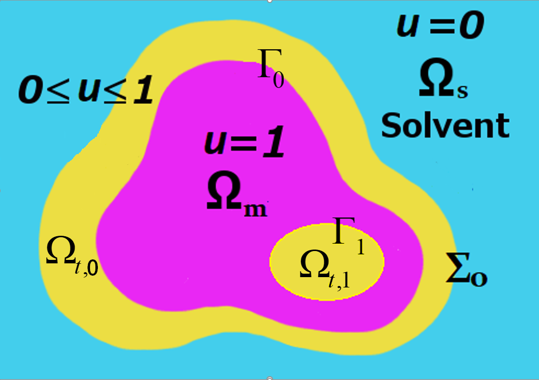
Figure 3. Illustration of a solute with one cavity inside.

6. Numerical Simulations

The non-differentiable structure of (2.11) and the Constraints (2.1) and (2.2) generate an essential difficulty in the numerical simulations of (2.11). This motives us to study a sequence of approximation problems.

6.1. An Approximation Problem

Recall the definition of $\{q_{k}\}_{k=1}^{\infty}$ from Section 3. We introduce a family of perturbed solvation free energy functionals

$$I_{k}(u)= \gamma\int_{\Omega}|\nabla u|^{q_{k}}\,dx+\int_{\Omega}\left[P_{h}u^{p}+\rho_{s}(1-u^{p})U^{\mathrm{vdW}}\right]\,dx$$

$$+\int_{\Omega}\left[\rho_{m}\psi-\frac{1}{2}\epsilon(u)|\nabla\psi|^{2}-(q_{k}-u^{p})B(\psi)\right]\,dx,$$ (6.1)

where $\psi\in\mathcal{A}$ satisfies (3.2). We will seek a minimizer of $I_{k}(\cdot)$ in $\mathcal{Y}_{k}$, c.f. (3.1). For notational brevity, we term the second line of (6.1) $I_{{\rm p},k}(u,\psi)$.

Let $u_{{\rm min}}$ be a minimizer of (2.11) in $\mathcal{Y}$ and $\psi_{{\rm min}}=\psi_{u_{{\rm min}}}$ be the solution of (2.10) with $u=u_{{\rm min}}$.

To prepare for the main result of this section, we introduce

$$\Omega_{j,k}:=\{x\in\Omega:{\rm dis}(x,\Omega_{j})<1/k\},\quad j\in\{m,s\}$$

and

$$\mathcal{X}_{k}:=\{u\in\mathcal{Y}:u\equiv 1\,\,\text{ in }\Omega_{m,k}\quad\text{and}\quad u\equiv 0\,\,\text{ in }\Omega_{s,k}\},\quad k\in\mathbb{N},$$

and quote the following two lemmas from [55].

Lemma 6.1.

([55, Lemma 2.6]) For every $f\in\mathcal{X}_{k}$, there exists a sequence $\{f_{n}\}_{n=1}^{\infty}\subset C^{\infty}(\overline{\Omega})$ satisfying Constraints (2.1) and (2.2) such that

• $f_{n}\to f$ in $L^{1}(\Omega)$, and

• $\|Df_{n}\|(\Omega)\to\|Df\|(\Omega)$ as $n\to\infty$.

Lemma 6.2.

([55, Lemma 2.7]) For every $f\in\mathcal{Y}$, we define $\{f_{k}\}_{k=1}^{\infty}\subset BV(\Omega)$ by

$$f_{k}(x)=\begin{cases}1,\quad&x\in\Omega_{m,k}\\ 0,&x\in\Omega_{s,k}\\ f(x),&\text{elsewhere}.\end{cases}$$

If $\Sigma_{i}\in C^{2}$ with $i\in\{0,1\}$, then

• $f_{k}\to f$ in $L^{1}(\Omega)$ and

• $\|Df_{k}\|(\Omega)\to\|Df\|(\Omega)$ as $k\to\infty$.

The theoretic basis of the numerical simulation is the following theorem.

Theorem 6.3.

For each $k=1,2,\cdots$, there exists a unique $u_{{\rm min},k}\in\mathcal{Y}_{k}\cap\mathcal{Y}$ such that $I_{k}(u_{{\rm min},k})=\underset{{u\in\mathcal{Y}_{k}}}{{\rm min}}I_{k}(u)$. If, in addition, $\Sigma_{i}\in C^{2}$, $i\in\{0,1\}$,

$$\lim\limits_{k\to\infty}I_{k}(u_{{\rm min},k})=I(u_{{\rm min}}),$$

and as $k\to\infty$

$$u_{{\rm min},k}\to u_{{\rm min}}\quad\text{in }L^{r}(\Omega)$$

for all $r\in[1,\infty)$ and

$$\psi_{{\rm min},k}\to\psi_{{\rm min}}\quad\text{in }H^{1}(\Omega),$$

where $\psi_{{\rm min},k}=\psi_{u_{{\rm min},k}}$ is the solution to (3.2) with $u=u_{{\rm min},k}$.

Proof.

(i) The existence and uniqueness of a minimizer $u_{{\rm min},k}\in\mathcal{Y}_{k}$ of $I_{k}(\cdot)$ for each $k$ can be proved in the same manner as in Theorem 4.1.

(ii) We will show that $u_{{\rm min},k}$ is a global minimizer of $I_{k}(\cdot)$ iff $(u_{{\rm min},k},\psi_{{\rm min},k})$ is a saddle point of

$$L_{k}(u,\psi):=\!\int_{\Omega}\left[\gamma|\nabla u|^{q_{k}}+P_{h}u^{p}+\rho_{s}(1-u^{p})U^{\mathrm{vdW}}\right]\,dx+\int_{\Omega}\left[\rho_{m}\psi-\frac{1}{2}\epsilon(u)|\nabla\psi|^{2}-(q_{k}-u^{p})B(\psi)\right]\,dx$$ (6.2)

in $\mathcal{Y}_{k}\times\mathscr{A}$, where

$$\mathscr{A}:=\{v\in\mathcal{A}:\|v\|_{H^{1}}\leq\widetilde{C}_{0}\text{ and }\|v\|_{\infty}\leq\widetilde{C}_{0}\}.$$

Here $\widetilde{C}_{0}$ is the constant in (3.3). Proposition 3.1 shows that $\psi_{{\rm min},k}\in\mathscr{A}$. Denote by $\mathcal{S}_{k}$ the set of all saddle points of $L_{k}$. Recall that $(u_{0},\psi_{0})\in\mathcal{S}_{k}$ iff

$$L_{k}(u_{0},\psi)\leq L_{k}(u_{0},\psi_{0})\leq L_{k}(u,\psi_{0}),\quad\forall(u,\psi)\in\mathcal{Y}_{k}\times\mathscr{A}.$$ (6.3)

It follows from Proposition 3.1 and Theorem 4.1 that

$$I_{k}(u_{{\rm min},k})=:M_{k}=\underset{{u\in\mathcal{Y}_{k}}}{{\rm min}}\underset{{\psi\in\mathscr{A}}}{{\rm max}}L_{k}(u,\psi).$$

Note that $\mathcal{Y}_{k}$ and $\mathscr{A}$ are closed and convex in $W^{1,q_{k}}(\Omega)$ and $H^{1}(\Omega)$, respectively. Moreover,

$$[u\mapsto L_{k}(u,\psi)]\text{ is strictly convex and lower semi-continuous }\forall\psi\in\mathscr{A},$$

and

$$[\psi\mapsto L_{k}(u,\psi)]\text{ is strictly concave and upper semi-continuous }\forall u\in\mathcal{Y}_{k}.$$

Since $\mathscr{A}$ is bounded in $H^{1}(\Omega)$, [29, Remark VI.2.3] implies that

$$\underset{{\psi\in\mathscr{A}}}{{\rm max}}\inf\limits_{u\in\mathcal{Y}_{k}}L_{k}(u,\psi)=\underset{{u\in\mathcal{Y}_{k}}}{{\rm min}}\underset{{\psi\in\mathscr{A}}}{{\rm max}}L_{k}(u,\psi)=M_{k}.$$

It follows from the direct method of Calculus of Variation that the infimum is achieved. Therefore,

$$\underset{{\psi\in\mathscr{A}}}{{\rm max}}\underset{{u\in\mathcal{Y}_{k}}}{{\rm min}}L_{k}(u,\psi)=\underset{{u\in\mathcal{Y}_{k}}}{{\rm min}}\underset{{\psi\in\mathscr{A}}}{{\rm max}}L_{k}(u,\psi)=L_{k}(u_{{\rm min},k},\psi_{{\rm min},k}).$$ (6.4)

By [29, Proposition VI.1.2], $(u_{{\rm min},k},\psi_{{\rm min},k})\in\mathcal{S}_{k}$. Conversely, if $(u_{0},\psi_{0})\in\mathcal{S}_{k}$, then (6.3) and Proposition 3.1 show that $\psi_{0}$ is the solution of (3.2) with $u=u_{0}$. What is more, since (6.4) still holds true if we replace $(u_{{\rm min},k},\psi_{{\rm min},k})$ by $(u_{0},\psi_{0})$, we infer that $u_{0}=u_{{\rm min},k}$.

If $\mathcal{L}^{3}(\{u_{{\rm min},k}>1\}\cup\{u_{{\rm min},k}<0\})>0$, define

$$\bar{u}_{{\rm min},k}(x)=\begin{cases}1,\quad&\text{if }u_{{\rm min},k}(x)>1,\\ 0,&\text{if }u_{{\rm min},k}(x)<0,\\ u_{{\rm min},k}(x),&\text{elsewhere.}\end{cases}$$

Then direct computations show that

$$L_{k}(\bar{u}_{{\rm min},k},\psi_{{\rm min},k})<L_{k}(u_{k},\psi_{{\rm min},k}).$$

A contradiction. Hence, $u_{{\rm min},k}\in\mathcal{Y}$.

(iii) Fix $v\in\mathcal{Y}_{k}$. Then, by (3.7), $G_{v}^{k}(\psi_{v})<\widetilde{C}_{1},$ where $\psi_{v}$ is the solution to (3.2) with $u=v$. Then

$$I_{k}(v)\leq\gamma\int_{\Omega}|\nabla v|^{q_{k}}\,dx+2P_{h}{\rm Vol}(\Omega)-\int_{\Omega\setminus\Omega_{s}}\rho_{s}U^{{\rm vdW}}\,dx+\widetilde{C}_{0}\|\rho_{m}\|_{\infty}{\rm Vol}(\Omega_{m})\leq C_{2},$$

where $\widetilde{C}_{0}$ is the constant in Proposition 3.1 and $C_{2}$ is independent of $k$ and $v$. This yields that

$$C_{2}\geq I_{k}(u_{{\rm min},k})\geq\gamma\int_{\Omega}|\nabla u_{{\rm min},k}|^{q_{k}}\,dx+P_{h}\|u_{{\rm min},k}\|_{p}^{p}+C_{3}-\widetilde{C}_{1}$$

$$\geq \gamma\|\nabla u_{{\rm min},k}\|_{1}^{q_{k}}\left({\rm Vol}(\Omega)\right)^{1-{q_{k}}}+P_{h}\|u_{{\rm min},k}\|_{p}^{p}+C_{3}-\widetilde{C}_{1},$$ (6.5)

where $C_{3}=\int_{\Omega\setminus\Omega_{m}}\rho_{s}U^{{\rm vdW}}\,dx$. We thus infer from (6.5) that

$$\|u_{{\rm min},k}\|_{W^{1,1}}=\|u_{{\rm min},k}\|_{BV}\leq C_{4}$$

for some $C_{4}$ independent of $k$. Proposition A.2 implies that there exists a subsequence of $\{u_{{\rm min},k}\}_{k=1}^{\infty}$, not relabelled, converging to some $u_{0}\in\mathcal{Y}$ in $L^{1}(\Omega)$. The Riesz-Thorin interpolation theorem then implies that $u_{{\rm min},k}\to u_{0}$ in $L^{r}(\Omega)$ for all $r\in[1,\infty)$ as $k\to\infty$. Note that

$$\int_{\Omega}|\nabla u_{{\rm min},k}|^{q_{k}}\,dx\geq\|\nabla u_{{\rm min},k}\|_{1}^{q_{k}}\left({\rm Vol}(\Omega)\right)^{1-{q_{k}}}.$$

Then it follows from Propositions A.3 and 3.2 that

$$I(u_{0})\leq\liminf\limits_{k\to\infty}I_{q_{k}}(u_{{\rm min},k}).$$

On the other hand, we define

$$w_{n}(x)=\begin{cases}1,\quad&x\in\Omega_{m,n}\\ 0,&x\in\Omega_{s,n}\\ u_{0}(x),&\text{elsewhere}.\end{cases}$$

We will show that

$$\limsup\limits_{k\to\infty}I_{k}(u_{{\rm min},k})\leq I(w_{n}).$$ (6.6)

Lemma 6.1 implies that we can find a sequence $\{w_{n,i}\}_{i=1}^{\infty}$ such that $w_{n,i}\in C^{\infty}(\overline{\Omega})\cap\mathcal{Y}_{k}$ for all $k$ and

$$w_{n,i}\to w_{n}\,\,\text{ in }L^{1}(\Omega)\quad\text{and}\quad\|Dw_{n,i}\|(\Omega)\to\|Dw_{n}\|(\Omega)\quad\text{as }i\to\infty.$$

Since $u_{{\rm min},k}$ minimizes $I_{k}(\cdot)$ in $\mathcal{Y}_{k}$, we have

$$I_{k}(u_{{\rm min},k})\leq I_{k}(w_{n,i}).$$

Pushing $k\to\infty$, the dominated convergence theorem and Proposition 3.2 imply that

$$\limsup\limits_{k\to\infty}I_{k}(u_{{\rm min},k})\leq I(w_{n,i}).$$

Then Lemma 6.1 and Proposition 3.2 immediately yield (6.6). Now Lemma 6.2 and Proposition 3.2 give that

$$\limsup\limits_{k\to\infty}I_{k}(u_{{\rm min},k})\leq I(u_{0}).$$

Finally, the convergence of $\psi_{{\rm min},k}$ is a direct consequence of Proposition 3.2.

(iv) Denote by $\psi_{k}$ the solution of (3.2) with $u=u_{{\rm min}}$. Then by Proposition 3.1,

$$I(u_{{\rm min}})\geq I_{\rm np}(u_{{\rm min}})+I_{\rm p}(u_{{\rm min}},\psi_{k})\geq I_{\rm np}(u_{{\rm min}})+I_{{\rm p},k}(u_{{\rm min}},\psi_{k})\geq I_{k}(u_{{\rm min},k}).$$

This yields

$$I(u_{{\rm min}})\geq\lim\limits_{k\to\infty}I_{k}(u_{{\rm min},k})=I(u_{0}).$$

By the uniqueness of a global minimizer of $I(\cdot)$, we conclude that $u_{0}=u_{{\rm min}}$. ∎

6.2. Variation of Solvation Free Energy

Motivated by Theorem 6.3, we will study the numerical simulations of the approximating functional (6.1). As the first step, we will derive the variational formulas of (6.1) at $u_{{\rm min},k}$. Recall that $u_{{\rm min},k}$ minimizes (6.1) in $\mathcal{Y}_{k}$ iff $(u_{{\rm min},k},\psi_{{\rm min},k})$ is a saddle point of (6.2) in $\mathcal{Y}_{k}\times\mathscr{A}$, where $\psi_{{\rm min},k}$ solves (3.2) with $u=u_{{\rm min},k}$. This means that

$$L_{k}(u_{{\rm min},k},\psi_{{\rm min},k})=\underset{{u\in\mathcal{Y}_{k}}}{{\rm min}}L_{k}(u,\psi_{{\rm min},k}).$$

Given any $\phi\in C^{\infty}_{0}(\Omega_{t})$, as $u_{{\rm min},k}\in\mathcal{Y}$, for sufficiently small $\delta>0$,

$$u_{{\rm min},k}+\varepsilon\phi\in\mathcal{Y}_{k},\quad|\varepsilon|<\delta.$$

Therefore, we can verify that $u_{{\rm min},k}$ satisfies

$$\gamma\int_{\Omega}q_{k}|\nabla u_{{\rm min},k}|^{q_{k}-2}\nabla u_{{\rm min},k}\cdot\nabla\phi\,dx+\int_{\Omega}\left[pu_{{\rm min},k}^{p-1}\left(P_{h}-\rho_{s}U^{\mathrm{vdW}}\right)\phi\right]\,dx$$

$$+ \int_{\Omega}\left[pu_{{\rm min},k}^{p-1}\left(B(\psi_{{\rm min},k})+\frac{\epsilon_{s}-\epsilon_{m}}{2}|\nabla\psi_{{\rm min},k}|^{2}\right)\phi\right]\,dx=0$$

for all $\phi\in C^{\infty}_{0}(\Omega_{t})$. Therefore, $u_{{\rm min},k}$ solves

$$\gamma q_{k}{\rm div}\left(|\nabla u|^{q_{k}-2}\nabla u\right)-pu^{p-1}V(\psi_{{\rm min},k})=0\quad\text{in }\Omega_{t}$$

in the weak sense, where

$$V(\psi)=P_{h}-\rho_{s}U^{\mathrm{vdW}}+B(\psi)+\frac{\epsilon_{s}-\epsilon_{m}}{2}|\nabla\psi|^{2}.$$

In view of (3.2), $(u_{{\rm min},k},\psi_{{\rm min},k})$ solves the following elliptic system

$$\left\{\begin{aligned} {\rm div}(\epsilon(u)\nabla\psi)+(q_{k}-u^{p})\sum\limits_{j=1}^{N_{c}}c_{j}^{\infty}q_{j}e^{-\beta\psi q_{j}}&=-\rho_{m}&&\text{in}&&\Omega;\\ \psi&=\psi_{\infty}&&\text{on}&&\partial\Omega;\\ \gamma q_{k}{\rm div}\left(|\nabla u|^{q_{k}-2}\nabla u\right)-pu^{p-1}V(\psi)&=0&&\text{in}&&\Omega_{t};\\ u&=1&&\text{on}&&\Sigma_{1};\\ u&=0&&\text{on}&&\Sigma_{0}.\end{aligned}\right.$$ (6.7)

Remark 6.4.

The approach in this section actually gives a solution to the variational analysis of (1) with Constraints 2.1 and 2.2, which provides a complete answer to a question in our previous work [55].

6.3. Computational methods

This section presents the computational methods and algorithms for the solution of the coupled system (6.7) and its associated parameterization process. The solution of (6.7) provides a physically sound “diffuse solute-solvent interface profile” $u$ and the electrostatic potential $\psi$, and thereby the calculation of the total solvation free energy.

While solving for $u$ and $\psi$, the surface evolution equation and the perturbed PB equation cannot be decoupled and thus need to be solved simultaneously. In the following, we first describe in more detail about the solution methods for each equation and their discretized formulations. Then the scheme for the convergence of two coupled equations is presented as well as a simple parameterization approach for optimal parameter values.

6.3.1. The perturbed Poisson-Boltzmann equation

For the solution of perturbed PB (PPB) equation, we adopted the finite difference scheme. Thanks to the continuous dielectric function, an accurate solution can be achieved with a standard second-order center difference scheme. Specifically, for a solvent without salt, the PPB equation can be simplified to a perturbed Poisson equation. If the position $(x_{i},y_{j},z_{k})$ is represented by the pixel $(i,j,k)$, its discretized form becomes

$$\epsilon(i+\frac{1}{2},j,k)[\psi(i+1,j,k)-\psi(i,j,k)] - \epsilon(i-\frac{1}{2},j,k)[\psi(i-1,j,k)-\psi(i,j,k)]$$

$$+\epsilon(i,j+\frac{1}{2},k)[\psi(i,j+1,k)-\psi(i,j,k)] - \epsilon(i,j-\frac{1}{2},k)[\psi(i,j-1,k)-\psi(i,j,k)]$$

$$+\epsilon(i,j,k+\frac{1}{2})[\psi(i,j,k+1)-\psi(i,j,k)] - \epsilon(i,j,k-\frac{1}{2})[\psi(i,j,k-1)-\psi(i,j,k)]=-q(i,j,k)/h$$

where the uniform grid spacing $h$ is applied at $x$, $y$ and $z$ directions, and $\epsilon(i+\frac{1}{2},j,k)=\epsilon(u(x_{i}+\frac{1}{2}h,y_{j},z_{k}))$, $q(i,j,k)$ is used to describe the fractional charge at grid point $(x_{i},y_{j},z_{k})$. The fractional charge is calculated by the second-order interpolation (trilinear) of the charge density $\rho_{m}$. Then a standard linear algebraic equation system is resulted from the the discretized perturbed Poisson equation in the form of $AX=B$, in which $X$ is the targeted solution. Matrix $A$ is the discretization matrix and $B$ is the source term according to the discrete charges.

The boundary condition of PPB equation is computed via the summation of electrostatic potential contributions of individual atom charges [33]. The resulted linear system can be solved by various linear solvers (like biconjugate gradient in this study) together with pre-conditioners for potential acceleration. $0$ can be used for the initial guess of the solution and convergence tolerance is set as a small number such as $10^{-6}$. It has been shown that the designed PB solver is capable of delivering second-order accuracy [17].

6.3.2. The surface evolution equation

The solution of the surface evolution equation can be attained via the following parabolic PDE as done in earlier work [7, 17].

$$\frac{\partial u}{\partial t}=|\nabla u|^{2-q_{k}}\left[{\rm div}\left(\gamma q_{k}\frac{\nabla u}{|\nabla u|^{2-q_{k}}}\right)+pu^{p-1}V\right],$$ (6.8)

As a result, the steady state solution of Equation (6.8) can be directly taken as the solution of the original elliptic equation.

Computationally, the equation (6.8) can be expanded into a form as follows.

$$\frac{\partial u}{\partial t}= \gamma q_{k}\frac{(u_{x}^{2}+u_{y}^{2}+(q_{k}-1)u_{z}^{2})u_{zz}+(u_{x}^{2}+(q_{k}-1)u_{y}^{2}+u_{z}^{2})u_{yy}+((q_{k}-1)u_{x}^{2}+u_{y}^{2}+u_{z}^{2})u_{xx}}{u_{x}^{2}+u_{y}^{2}+u_{z}^{2}}$$ (6.9)

$$-\gamma(2-q_{k})q_{k}\frac{2u_{x}u_{y}u_{xy}+2u_{x}u_{z}u_{xz}+2u_{z}u_{y}u_{yz}}{u_{x}^{2}+u_{y}^{2}+u_{z}^{2}}$$

$$+\left(\sqrt{u_{x}^{2}+u_{y}^{2}+u_{z}^{2}}\right)^{2-q_{k}}pu^{p-1}V.$$

In particular, the time-dependent derivative is carried out by explicit Euler scheme. Note that other implicit schemes can be designed to improve the solution efficiency and will be pursued later. The first and second order spatial derivatives are handled by finite difference schemes [17]. To impose the domain decomposition in (6.7), we let $u$ be fixed as one in the pure solute area $\Omega_{m}$ and as zero in the pure solvent region $\Omega_{s}$. Here the pure solute area is numerically defined to be enclosed by a smoothed Van Der Waals surface (vdW) and the the pure solvent region is the area outside a smoothed solvent accessible surface (SAS). The initial value of $u$ in between $\Omega_{m}$ and $\Omega_{s}$ can be set between 0 and 1.

6.3.3. Coupling of the perturbed Poisson Boltzmann and surface evolution equations

In principle, the surface evolution equation needs to be solved simultaneously with the perturbed PB equation until the solution process reaches a self-consistency. To speed up the whole iterative process, electrostatic potential $\psi$ is updated after a number of time steps (i.e., 10 to 100 steps) evolution of the parabolic surface equation [17].

Moreover, a simple relaxation algorithm is adopted to guarantee the convergence of the iterative process as follows [17] :

$$u=\alpha u_{new}+(1-\alpha)u_{old}, \quad 0<\alpha<1,$$ (6.10)

$$\psi=\alpha^{\prime}\psi_{\rm new}+(1-\alpha^{\prime})\psi_{\rm old}, \quad 0<\alpha^{\prime}<1,$$ (6.11)

where $u_{new}$ and $u_{old}$ are the new and old $u$ profile values from current and previous steps, respectively. $\psi_{\rm old}$ and $\psi_{\rm new}$ denote previous and new electrostatic potentials, respectively. $\alpha=0.5$ and $\alpha^{\prime}=0.5$ are set in our calculation.

In addition, a simple cutoff strategy is conducted to apply Constraint (2.1) and to avoid possible numerical errors:

$$u=\begin{cases}u(x)\quad&u\in[0,1]\\ 0&u<0\\ 1&u>1.\end{cases}$$ (6.12)

The cutoff checkup is carried out every time step or several steps during the solution of surface evolution equation.

Finally, to reduces the total iteration number and save the computational time significantly, first of all, one may start the iterative process with an initial $u$ from solving Eq. (6.8) without the electrostatic potential term. Second, one may take the prior potential $\psi$ as a good guess for the next resulted linear system in the PPB solution. That will make the PPB solver converge faster.

6.3.4. Parameterization

There are some parameter values that need to be determined for real numerical simulations of solvation free energy. They include solvent density $\rho_{s}$, the solvent radius $\sigma_{s}$,$\gamma$, $P_{h}$ and so on. Since most of the parameters are involved in nonpolar solvation energy, a previous simple parameter fitting strategy is adopted here [19, 55]. In particular, on the one side, some parameter values are fixed or given such as: $\rho_{s}$=0.03341/ų; solvent radius $\sigma_{s}$ =0.65 Š; radii of solute atoms like $\sigma_{c}$ =1.87 Š. On the other side, some are considered as fitting parameters like $\gamma$, $P_{h}$, and well depth parameters $\epsilon_{is}$ where $i$ denotes different atom types. The following iterative procedure is used to obtain the optimal fitting parameter values:

Step 0: An initial guess of fitting parameters and a trial set of molecules are determined with their existing informaion such as atomic coordinates, radii, and experimental data of solvation free energies.

Step 1: For individual $j$-th molecule, $j=1,\cdots N_{m}$ where $N_{m}$ is the total number of molecules in the trial set, the coupled system (6.7) is solved until self-consistency is reached to find the quasi-steady state solution of $u_{j}$ and $\psi_{j}$ with latest parameter values. Note that if the trial set is nonpolar, one only needs to solve the surface evolution equation without a driven potential from the electrostatic field. Then the fitting process is exactly the same as our previous paper [55].

Step 2: Electrostatic solvation energy $I_{p,q_{k}}^{j}$ is calculated for each molecules using the profile of $\psi_{j}$.

Step 3: A non-negative least squares algorithm is used to update all non-negative parameters $P_{h}$, $\gamma$, and $\epsilon_{is}$ with a minimization problem

$$T=\underset{(p,\gamma,\epsilon_{is})}{{\rm min}}\sum\limits_{j=1}^{N_{m}}\left(I_{np,q_{k}}^{j}+I_{p,q_{k}}^{j}-I_{q_{k}}^{j,\rm exp}\right)^{2},$$

where $I_{q_{k}}^{j,\rm exp}$ is the existing experimental data of solvation free energies in the literature.

Step 4: The iterative loop from Step 1 to Step 3 is repeated until all fitting parameters converge to a certain set of values within a pre-set tolerance.

6.4. Simulation Results

In this section, both nonpolar and polar molecules are taken for the numerical simulation and model validation. Nonpolar molecules are simulated first to justify the usage of $u^{p}$ which represents the volume ratio of solute. That may minimize modeling uncertainties from solvent-solute electrostatic interactions. It is followed by the calculation of polar molecules to demonstrate the potential of current proposed model for the prediction of polar solvation energies.

6.4.1. Nonpolar molecules

To validate the current constrained variational model, we start with a set of 11 alkanes as a calibration set for numerical implementation of model solution and the associated parameterizaton process. First of all, two parameters $N$ and $q_{k}$ need to be pre-determined for each simulation. It turns out that optimal fitting parameters are uniquely computed for a set of arbitrary $N>1$ and $q_{k}$, where $p=\frac{2N}{2N-1}$, and $q_{k}\to 1^{+}$. For instance, when $N=40$ and $q_{k}=1.00001$, the calculated optimal fitting parameters are the following: $\gamma=0.0746$ kcal/(mol Ų), $P_{h}=0.0090$ kcal/(mol ų) and $\epsilon_{cs}=0.486$ kcal/mol, and $\epsilon_{hs}=0.00$ kcal/mol. Note that $\epsilon_{hs}$ and $\epsilon_{cs}$ are well depth parameters of the hydrogen and carbon, respectively. Moreover, it is shown that the current model is able to reproduce the total solvation free energies of 11 alkanes very well (see Table 1). The root mean square (RMS) error of 11 alkenes is 0.109 kcal/mol. For the nonpolar solvation free energy, the repulsive and attractive parts of solvation free energy are also calculated for detailed comparisons with others in the literature. Note that the first two terms of (2.3) are considered as the repulsive part of solvation free energy.

Table 1. Computed total solvation free energies of the trial set of 11 alkane compounds and their repulsive and attractive decomposition when $q_{k}=1.00001$. $\gamma=0.0746$ kcal/(mol Ų), $P_{h}=0.0090$ kcal/(mol ų) and $\epsilon_{cs}=0.486$ kcal/mol, and $\epsilon_{hs}=0.00$ kcal/mol

Compound	Rep. part	Att. part	Numerical	Experimental [11]
	(kcal/mol)
methane	4.21	-2.21	2.00	2.00
ethane	5.90	-3.95	1.95	1.83
propane	9.00	-6.89	2.12	1.96
butane	7.45	-5.42	2.03	2.08
pentane	10.58	-8.27	2.30	2.33
hexane	12.13	-9.75	2.38	2.49
isobutane	8.90	-6.64	2.26	2.52
2-methylbutane	10.20	-7.80	2.40	2.38
neopentane	10.21	-7.61	2.60	2.50
cyclopentane	9.21	-8.04	1.17	1.20
cyclohexane	10.45	-9.08	1.37	1.23
RMS of calibration set			0.109

Next, it is interesting to see whether the model parameter $N$ or equivalently $p=\frac{2N}{2N-1}$, which is introduced in the volume ratio of solute $u^{p}$, plays an important role in the solvation free energy calculation and prediction. For this purpose, different $N$ values are chosen for the set of 11 alkanes while fixing all other simulation setting. It is evident that almost identical simulation results are obtained for large enough $N$ (See Table 2).

Table 2. Different optimized parameters and RMS errors for various $N$ values when $q_{k}=1.00001$

$q$ value	$\gamma$ (kcal/(mol Å2))	$P_{h}$ (kcal/(mol Å3))	$\epsilon_{cs}$ (kcal/mol)	RMS (kcal/mol)
1	0.0758	0.0078	0.493	0.105
2	0.0749	0.0085	0.487	0.108
5	0.0746	0.009	0.486	0.109
10	0.0746	0.009	0.486	0.109
20	0.0746	0.009	0.486	0.109
40	0.0746	0.009	0.486	0.109

Moreover, with $q=1.00001$ and $N=40$, a predictive study is conducted for a set of 11 alkene compounds which was also used before [53, 19, 55]. The assumed similar solvent environment allows one to apply the above-obtained optimized parameters of 11 alkanes here because of the fact that both nonpolar sets only possess two types of atoms (C and H). It turns out that the numerical prediction of the current model matches the experimental data well as shown in Table 3. The RMS error of 11 alkenes is 0.21 kcal/mol.

Table 3. Computed total solvation free energies of 11 alkene compounds when $q=1.00001$ and $N=40$.

Compound	Rep. part	Att. part	Numerical	Experimental [53]
	(kcal/mol)
3-methyl-1- butene	10.15	-8.32	1.84	1.82
1-butene	8.68	-7.04	1.64	1.38
ethene	5.51	-4.12	1.49	1.27
1-heptene	13.42	-11.58	1.84	1.66
1-hexene	11.83	-10.05	1.78	1.68
1-nonene	16.64	-14.59	1.95	2.06
2-methyl-2-butene	10.08	-8.33	1.74	1.31
1-octene	14.99	-13.01	1.98	2.17
1-pentene	10.22	-8.58	1.65	1.66
1-propene	7.12	-5.59	1.53	1.27
trans-2-heptene	13.45	-11.62	1.83	1.66
RMS of prediction set			0.209

Furthermore, we have theoretically proved that total solvation energies converge to the case of $q_{k}=1$ when $q_{k}\to 1^{+}$. Numerically, the convergence can be demonstrated as follow: choosing a set of molecules like the above alkene compounds and fixing all other numerical settings, one allows the value of $q_{k}$ to approach 1 by creating a sequence of $q_{k}$ ($q_{k}=1.01,1.001,1.0001,1.00001,1.000001$). Then the total solvation free energy of each molecule is computed. Table 4 illustrates the convergence of total solvation free energies for all eleven alkenes.

Table 4. Convergence of total solvation free energies of of eleven alkene molecules when $q\to 1^{+}$ with other parameter values fixed.

Compound	1.01	1.001	1.0001	1.00001	1.000001
	(kcal/mol)
3-methyl-1- butene	2.567	1.908	1.844	1.837	1.837
1-butene	2.268	1.701	1.647	1.641	1.641
ethene	1.888	1.524	1.489	1.485	1.485
1-heptene	2.797	1.930	1.846	1.837	1.837
1-hexene	2.625	1.857	1.784	1.776	1.775
1-nonene	3.126	2.060	1.957	1.946	1.946
2-methyl-2-butene	2.468	1.751	1.744	1.745	1.745
1-octene	3.049	2.083	1.990	1.980	1.980
1-pentene	2.381	1.716	1.653	1.646	1.645
1-propene	2.043	1.575	1.530	1.525	1.525
trans-2-heptene	2.789	1.918	1.835	1.826	1.826

Remark that regarding the numerical calculation of solvation free energy for nonpolar molecules, the currently computed results are almost the same as the previous constrained solvation model [55] when $N$ is large enough. The similarity can be explained by the fact that $pu^{p-1}\to 1$ for $0<u<1$ when $p=\frac{2N}{2N-1}\to 1$ with $N\to\infty$.

6.4.2. Polar molecules

The introduction of $u^{p}$ as solute volume ratio enables us to derive the system (6.7) from proposed constrained total solvation energy model (2.11). It has been a theoretical advance from our previous constrained model in which a PDE was derived only for nonpolar energy functional due to the complex two-obstacle problem [55].

In this section, the model potential and validation are demonstrated numerically for polar molecules. To the end, a challenging set of 17 compounds is chosen. The challenge arises partially due to strong solvent-solute interactions caused by polyfunctional or interacting polar groups. Actually, its challenge can be seen quantitatively. For instance, using an explicit solvent model, Nicholls et al. obtained the root mean square error (RMS) as $1.71\pm 0.05$ kcal/mol via [50]. With an improved multiscale model equipped with self-consistent quantum charge density by Chen et al [18], RMS was still around 1.50 kcal/mol.

For the current simulation, the structure data of the set of 17 molecules is taken from the supporting information of the paper of Nicholls et al [50] as we did before. The dielectric constants are slightly adjusted. In the solute region $\epsilon_{m}\approx 1$, while $\epsilon_{s}\leq 80$ for the solvent region. For this 17 set, different well-depth parameters $\epsilon_{is}$ need to be optimized based on the above-described simple parameterization scheme. It is shown that the computed solvation free energy is quite comparable with the experimental data. The root mean square error can be improved to 1.107 kcal/mol (See table 5) when $\epsilon_{m}=1.15$ and $\epsilon_{s}=70$. In addition, it is found that almost identical simulation results are obtained for large enough $N$. In other words, model parameter value $N$ does not play an important role for the solvation energy prediction while it obviously benefits the theoretical derivation and the proof for current constrained variational model. The minor effect of different $N$ values can be found in Table 6.

Table 5. Comparison of total free energies (kcal/mol) for 17 compounds

Compound	$\Delta G$	Exptl	Error
glycerol triacetate	-10.10	-8.84	-1.26
benzyl bromide	-2.38	-2.38	0.00
benzyl chloride	-3.95	-1.93	-2.02
m-bis(trifluoromethyl)benzene	1.07	1.07	0.00
N,N-dimethyl-p-methoxybenzamide	-8.74	-11.01	2.27
N,N-4-trimethylbenzamide	-8.60	-9.76	1.16
bis-2-chloroethyl ether	-3.26	-4.23	0.97
1,1-diacetoxyethane	-5.49	-4.97	-0.52
1,1-diethoxyethane	-4.51	-3.28	-1.23
1,4-dioxane	-4.84	-5.05	0.21
diethyl propanedioate	-5.10	-6.00	-0.90
dimethoxymethane	-1.28	-2.93	1.65
ethylene glycol diacetate	-6.48	-6.34	-0.14
1,2-diethoxyethane	-4.64	-3.54	-1.10
diethyl sulfide	-1.43	-1.43	0.00
phenyl formate	-4.35	-4.08	-0.27
imidazole	-10.83	-9.81	-1.02
RMS of 17 polar molecules		1.107

Table 6. Some optimized parameters and RMS errors from various $N$ values when $q_{k}=1.00001$

$q$ value	$\gamma$ (kcal/(mol Å2))	$P_{h}$ (kcal/(mol Å3))	$\epsilon_{cs}$ (kcal/mol)	RMS (kcal/mol)
4	0.314	0.000	1.105	1.107
8	0.314	0.000	1.105	1.107
16	0.314	0.000	1.105	1.107
32	0.314	0.000	1.105	1.107

7. Conclusions

Variational implicit solvation models (VISM) with diffuse solvent-solute interface definition have been considered as a successful approach to compute the disposition of an interface separating the solute and the solvent. It has been shown numerically that variational diffuse-interface solvation models can significantly improve the accuracy and efficiency of solvation energy computation. However, there are several open questions concerning those models at a theoretic level. In particular, all existing VISMs in literature lack the uniqueness of an energy minimizing solute-solvent interface and thus prevent us from studying many important properties of the interface profile.

Therefore, by introducing a new volume ratio function $u^{p}$, in this work, we have developed a novel constrained VISM based on a promising previously-proposed total variation based model (TVBVISM). Existence, uniqueness and regularity of the energy minimizing solute-solvent interface have been studied. Moreover, with the assistance of the precise depiction of the interface profile, this work provides a partial answer to the question why the solvation free energy is not minimized by a sharp solute-solvent interface. It turns out that when the mean curvature of $\Sigma_{0}$ is positive at some point, the energy minimizing state is never achieved by a sharp interface.

In addition, for the variational analysis of the new model and for the numerical computation of the solvation energy, a novel approach has been proposed to overcome the essential difficulty generated by the involved constraints in the model. Specifically, the variational formulas of the new energy functional can be rigorously derived via the introduction of the new volume ratio function $u^{p}$ together with an approximation technique by a sequence of $q$-energy type functionals. This is another advance from our previous work in which only the numerical study of nonpolar energy can be conducted for a constrained VISM. Model validation and numerical implementation have been demonstrated by using several common biomolecular modeling tasks. Numerical simulations show that the solvation energies calculated from our new model match the experimental data very well.

For the future work, we will provide a complete proof for the continuous dependence of the solvation free energy on the surfaces $\Omega_{m}$ and $\Omega_{s}$ in a suitable topology. Numerically, based on the derived elliptic system, we intend to further improve the accuracy and efficiency of the solvation energy prediction via refined parameterization schemes. Moreover, analysis of the current and potential numerical schemes like convergence will be a topic for future study.

Appendix A BV-functions

In Appendix A, we will introduce some notations and preliminaries of $BV-$functions. The main reference is [30, 1]. Let $\Omega\subset\mathbb{R}^{N}$ be open.

Definition A.1.

The space of functions of bounded variations on $\Omega$, denoted by $BV(\Omega)$, is the collections of all $L^{1}(\Omega)-$functions whose gradient $Df$ in the sense of distributions is a (vector-valued) Radon measure with finite total variation in $\Omega$. The total variation of $f$ in $\Omega$ is defined by

$$\sup\left\{\int_{\Omega}f{\rm div}z\,dx:\,z\in C_{0}^{\infty}(\Omega;\mathbb{R}^{N}),\,\|z\|_{\infty}\leq 1\right\}$$

and is denoted by $\|Df\|(\Omega)$ or $\int_{\Omega}\,d|Df|$. $BV(\Omega)$ is a Banach space endowed with the norm

$$\|f\|_{BV}:=\|f\|_{1}+\|Df\|(\Omega).$$

By the structure theorem of $BV-$functions, for every $f\in BV(\Omega)$, there exist Radon measure $\mu$ and a $\mu-$measurable function $\sigma:\Omega\to\mathbb{R}^{N}$ such that

• $|\sigma(x)|=1$ a.e. and

• $\int_{\Omega}f{\rm div}z\,dx=-\int_{\Omega}z\cdot\sigma\,d\mu$ for all $z\in C_{0}^{\infty}(\Omega;\mathbb{R}^{N})$.

We write $|Df|$ for the measure $\mu$.

Sobolev embedding also holds for functions of bounded variations:

$$BV(\Omega)\hookrightarrow L^{p}(\Omega),\quad\text{for all }1\leq p\leq 1^{*}=\frac{N}{N-1}.$$ (A.1)

The embedding is compact when $1\leq p<1^{*}$.

Proposition A.2.

Let $\Omega$ be bounded and with Lipschitz boundary. Assume that $\{f_{n}\}_{n=1}^{\infty}\subset BV(\Omega)$ satisfies

$$\sup\limits_{n}\|f_{n}\|_{BV}<\infty.$$

Then there exists a subsequence, not relabelled, such that

$$f_{n}\to f\quad\text{in }L^{1}(\Omega)\quad\text{for some }f\in BV(\Omega).$$

Proposition A.3.

Suppose that $\{f_{n}\}_{n=1}^{\infty}\subset BV(\Omega)$ and $f_{n}\to f$ in $L^{1}_{loc}(\Omega)$. Then

$$\|Df\|(\Omega)\leq\liminf\limits_{n\to\infty}\|Df_{n}\|(\Omega).$$

An Lebesgue measurable set $E\subset\mathbb{R}^{N}$ is said to have finite perimeter in $\Omega$ if

$$\chi_{E}\in BV(\Omega).$$

${\rm Per}(E;\Omega):=\|D\chi_{E}\|(\Omega)$ is called the perimeter of $E$ in $\Omega$.

Definition A.4.

Let $E$ be of finite perimeter in $\Omega$. We call the reduced boundary $\partial E^{*}$ the collection of all points $x\in{\rm supp}|D\chi_{E}|\cap\Omega$ such that the limit

$$\nu_{E}(x):=-\lim\limits_{r\to 0^{+}}\frac{D\chi_{E}(B(x,r))}{\|D\chi_{E}\|(B(x,r))}$$

exists in $\mathbb{R}^{N}$ and satisfies $|\nu_{E}|(x)=1$ a.e.. The function $\nu_{E}:\partial E^{*}\to\mathbb{S}^{N-1}$ is called the generalized outer normal to $E$. $\partial E\setminus\partial E^{*}$ is called the singular set of $E$. In particular, we have

$${\rm Per}(E;\mathbb{R}^{N}\setminus\partial E^{*})=0.$$ (A.2)

Proposition A.5.

Let $\Omega$ be bounded and with Lipschitz boundary. There is a bounded linear map

$${\rm Tr}:BV(\Omega)\to L^{1}(\partial\Omega)$$

such that

$$\int_{\Omega}f{\rm div}\phi\,dx=-\int_{\Omega}\phi\cdot Df+\int_{\partial\Omega}(\phi\cdot\nu){\rm Tr}f\,d\mathcal{H}^{N-1},$$

where $\nu$ is the outer unit normal on $\partial\Omega$. It is understood that the measure on $\partial\Omega$ is $\mathcal{H}^{N-1}$. The function ${\rm Tr}f$, which is uniquely defined $\mathcal{H}^{N-1}$ a.e. on $\partial\Omega$, is called the trace of $f$ on $\partial\Omega$.

Proposition A.6.

Let $\Omega$ be bounded and Lipschitz. Assume that $f_{1}\in BV(\Omega)$ and $f_{2}\in BV(\mathbb{R}^{N}\setminus\overline{\Omega})$. Define

$$f(x)=\begin{cases}f_{1}(x)\quad&x\in\Omega\\ f_{2}(x)&x\in\mathbb{R}^{N}\setminus\overline{\Omega}.\end{cases}$$

Then $f\in BV(\mathbb{R}^{N})$. Moreover,

$$\|Df\|(\mathbb{R}^{N})=\|Df_{1}\|(\Omega)+\|Df_{2}\|(\mathbb{R}^{N}\setminus\overline{\Omega})+\int_{\partial\Omega}|{\rm Tr}f_{1}-{\rm Tr}f_{2}|\,d\mathcal{H}^{N-1}.$$

Given $f\in L^{1}_{loc}(\Omega)$, we say that $f$ has an approximate limit at $x\in\Omega$ if there exists $z\in\mathbb{R}$ such that

$$\lim\limits_{r\to 0^{+}}\frac{1}{|B(x,r)|}\int_{B(x,r)}|u(y)-z|\,dy=0.$$ (A.3)

The set of points where this does not hold is called the approximate discontinuity set of $f$, and it is denoted by $S_{f}$. By Lebesgue differentiation theorem, $\mathcal{L}^{N}(S_{f})=0$. $z$ is uniquely determined via (A.3) and is denoted by $\tilde{f}(x)$. $f$ is said to be approximately continuous at $x$ if $x\notin S_{f}$ and $f(x)=\tilde{f}(x)$.

We say $f\in L^{1}_{loc}(\Omega)$ has an approximate jump point at $x\in\Omega$ if there exist $a\neq b\in\mathbb{R}$ and $\mu\in\mathbb{S}^{N-1}$ such that $a\neq b$ and

$$\lim\limits_{r\to 0^{+}}\frac{1}{|B(x,r)|}\int_{B^{+}_{\nu}(x,r)}|f(y)-a|\,dy=0\quad\text{and}\quad\lim\limits_{r\to 0^{+}}\frac{1}{|B(x,r)|}\int_{B^{-}_{\nu}(x,r)}|f(y)-b|\,dy=0.$$

Here

$$\begin{cases}B^{+}_{\nu}(x,r):=&\{y\in B(x,r):\,\nu\cdot(y-x)>0\}\\ B^{-}_{\nu}(x,r):=&\{y\in B(x,r):\,\nu\cdot(y-x)<0\}.\end{cases}$$

The set of all approximate jump points of $f$ is denoted by $J_{f}$. When $f\in BV(\Omega)$, $S_{f}$ is countably $\mathcal{H}^{N-1}-$rectifiable and $J_{f}$ is a Borel subset of $S_{f}$. Further $\mathcal{H}^{N-1}(S_{f}\setminus J_{f})=0$.

If $f\in BV(\Omega)$, we define the super-level sets of $f$ by

$$E_{t}:=\{f>t\},\quad t\in\mathbb{R}.$$

Then for $\mathcal{L}^{1}-$a.a. $t$, $E_{t}$ is of finite perimeter and the function

$$[t\mapsto{\rm Per}(E_{t};\Omega)]$$

is $\mathcal{L}^{1}-$measurable. Moreover, the coarea formula holds:

$$\int_{\Omega}v(x)d|Du|=\int_{-\infty}^{\infty}\int_{\Omega}v(x)d|D\chi_{E_{t}}|\,dt$$ (A.4)

for all $|Du|-$integrable function $v:\Omega\to\mathbb{R}$. In addition,

$$J_{f}=\bigcup\limits_{t_{1},t_{2}\in\mathbb{Q},\,t_{1}<t_{2}}\partial E_{t_{1}}\cap\partial E_{t_{2}}.$$ (A.5)

If $E\subset\mathbb{R}^{N}$ is measurable, we can define the upper and lower density of $E$ at $x$ by

$$\overline{D}(E,x)=\limsup\limits_{r\to 0^{+}}\frac{|E\cap B(x,r)|}{|B(x,r)|}\quad\text{and}\quad\underline{D}(E,x)=\liminf\limits_{r\to 0^{+}}\frac{|E\cap B(x,r)|}{|B(x,r)|},$$

respectively. If $u\in BV(\Omega)$, we define

$$u^{*}(x)=\inf\{s:\,\overline{D}(\{u\geq s\},x)=0\}\quad\text{and}\quad u_{*}(x)=\sup\{s:\,\underline{D}(\{u\leq s\},x)=0\}.$$

Then $u$ is approximately continuous at $x\in\Omega$ iff $u^{*}(x)=u_{*}(x)$.

Appendix B Tools from convex analysis

In Appendix B, we will state some useful tools from Convex Analysis. Interested readers may refer to the books [29, 58] for more details.

Let $X$ be a Banach space with norm $\|\cdot\|$. Throughout, we assume that $f:X\to\mathbb{R}\cup\{\pm\infty\}$ is convex and lower semicontinuous (l.s.c.) function. Its effective domain is defined by is

$${\rm dom}(f)=\{u\in X:\,f(u)<+\infty\}.$$

$f$ is said to be proper if it nowhere takes value $-\infty$ and is not identically equal to $+\infty$ on $X$.

Given any subset $U\subset X$, its indicator function $I_{U}$ is defined by

$$I_{U}(x)=\begin{cases}0\quad&\text{when }x\in U\\ \infty&\text{when }x\in X\setminus U.\end{cases}$$ (B.1)

We denote by $X^{*}$ the topological dual of $X$ and $\langle\cdot,\cdot\rangle$ the duality pairing. When $f$ is proper, the subdifferential of $f$ at $u\in{\rm dom}(f)$ is the set of all $u^{*}\in X^{*}$ such that

$$\langle u^{*},v-u\rangle\leq f(v)-f(u),\quad\forall v\in X,$$

and is denoted by $\partial f(u)$. Each element of $\partial f(u)$ is called a subdifferential of $f$ at $u$. When $\partial f(u)\neq\emptyset$, we say that $f$ is subdifferentiable at $u$.

The relationship between subdifferentiability and Gâteaux-differentiability is described by the following proposition.

Proposition B.1.

Let $f:X\to\mathbb{R}\cup\{+\infty\}$ be convex and proper. If $f$ is Gâteaux-differentiable at $u\in{\rm int}({\rm dom}(f))$, then $\partial f(u)=f^{\prime}(u)$, where $f^{\prime}(u)$ is the Gâteaux-derivative of $f$ at $u$.

By the definition of the subdifferential, it is obvious that

$$\partial f_{1}(v)+\partial f_{2}(v)\subseteq\partial(f_{1}+f_{2})(v).$$

However, the converse is not always true. We list below several cases where the converse holds.

Proposition B.2.

Suppose that $f_{1},f_{2}:X\to\mathbb{R}\cup\{+\infty\}$ is convex and l.s.c. and $u\in{\rm dom}(F_{1})\cap{\rm dom}(F_{2})$. If $f_{2}$ is continuous at $u$, then

$$\partial f_{1}(v)+\partial f_{2}(v)=\partial(f_{1}+f_{2})(v)\quad\forall v\in X.$$

Proposition B.3.

Let $f,g:X\to\mathbb{R}\cup\{\infty\}$ be proper, l.s.c. and convex functions such that

$$\bigcup\limits_{\mu>0}\mu({\rm dom}(f)-{\rm dom}(g))\text{ is a closed linear subspace of }X,$$

then

$$\partial(f+g)(u)=\partial f(u)+\partial g(u)\quad\forall u\in{\rm dom}(f)\cap{\rm dom}(g).$$

Proof.

This is [4, Corollary 2.1]. See also [62] for an easy proof. ∎

Literature cited

Literature cited

- [1] Luigi Ambrosio, Nicola Fusco, and Diego Pallara. Functions of bounded variation and free discontinuity problems. Oxford Mathematical Monographs. The Clarendon Press, Oxford University Press, New York, 2000.
- [2] D. Andelman. Chapter 12 - electrostatic properties of membranes: The poisson-boltzmann theory. In R. Lipowsky and E. Sackmann, editors, Structure and Dynamics of Membranes, volume 1 of Handbook of Biological Physics, pages 603–642. North-Holland, 1995.
- [3] Gabriele Anzellotti. Pairings between measures and bounded functions and compensated compactness. Ann. Mat. Pura Appl. (4), 135:293–318 (1984), 1983.
- [4] Hédy Attouch and Haïm Brezis. Duality for the sum of convex functions in general Banach spaces. In Aspects of mathematics and its applications, volume 34 of North-Holland Math. Library, pages 125–133. North-Holland, Amsterdam, 1986.
- [5] N. A. Baker. Improving implicit solvent simulations: a Poisson-centric view. Current Opinion in Structural Biology, 15(2):137–43, 2005.
- [6] Nathan A. Baker, David Sept, Simpson Joseph, Michael J. Holst, and J. Andrew McCammon. Electrostatics of nanosystems: Application to microtubules and the ribosome. Proceedings of the National Academy of Sciences, 98(18):10037–10041, 2001.
- [7] P. W. Bates, Z. Chen, Y. H. Sun, G. W. Wei, and S. Zhao. Geometric and potential driving formation and evolution of biomolecular surfaces. J. Math. Biol., 59:193–231, 2009.
- [8] P. W. Bates, G. W. Wei, and Shan Zhao. Minimal molecular surfaces and their applications. Journal of Computational Chemistry, 29(3):380–91, 2008.
- [9] A. H. Boschitsch and M. O. Fenley. Hybrid boundary element and finite difference method for solving the nonlinear Poisson-Boltzmann equation. Journal of Computational Chemistry, 25(7):935–955, 2004.
- [10] Wesley M. Botello-Smith, Xingping Liu, Qin Cai, Zhilin Li, Hongkai Zhao, and Ray Luo. Numerical poisson–boltzmann model for continuum membrane systems. Chemical Physics Letters, 555:274–281, 2013.
- [11] S. Cabani, P. Gianni, V Mollica, and L Lepori. Group Contributions to the Thermodynamic Properties of Non-Ionic Organic Solutes in Dilute Aqueous Solution. Journal of Solution Chemistry, 10(8):563–595, 1981.
- [12] V. Caselles, K. Jalalzai, and M. Novaga. On the jump set of solutions of the total variation flow. Rend. Semin. Mat. Univ. Padova, 130:155–168, 2013.
- [13] Vicent Caselles, Antonin Chambolle, and Matteo Novaga. The discontinuity set of solutions of the TV denoising problem and some extensions. Multiscale Model. Simul., 6(3):879–894, 2007.
- [14] Vicent Caselles, Antonin Chambolle, and Matteo Novaga. Regularity for solutions of the total variation denoising problem. Rev. Mat. Iberoam., 27(1):233–252, 2011.
- [15] Jianwei Che, Joachim Dzubiella, Bo Li, and J. Andrew McCammon. Electrostatic free energy and its variations in implicit solvent models. The Journal of Physical Chemistry B, 112(10):3058–3069, 2008. PMID: 18275182.
- [16] C. J. Chen, Rishu Saxena, and G. W. Wei. Differential geometry based multiscale models for virus formation and evolution. Int. J. Biomed. Imaging, 2010(308627), 2010.
- [17] Z. Chen, N. A. Baker, and G. W. Wei. Differential geometry based solvation models I: Eulerian formulation. J. Comput. Phys., 229:8231–8258, 2010.
- [18] Z. Chen and G. W. Wei. Differential geometry based solvation models III: Quantum formulation. J. Chem. Phys., 135:1941108, 2011.
- [19] Zhan Chen. Minimization and eulerian formulation of differential geormetry based nonpolar multiscale solvation models. Computational and Mathematical Biophysics, 1(open-issue), 2016.
- [20] Zhan Chen, Shan Zhao, Jaehun Chun, Dennis G. Thomas, Nathan A. Baker, Peter W. Bates, and G. W. Wei. Variational approach for nonpolar solvation analysis. The Journal of Chemical Physics, 137(8):084101, 2012.
- [21] L. T. Cheng, Joachim Dzubiella, Andrew J. McCammon, and B. Li. Application of the level-set method to the implicit solvation of nonpolar molecules. Journal of Chemical Physics, 127(8), 2007.
- [22] Shibin Dai, Bo Li, and Jianfeng Lu. Convergence of phase-field free energy and boundary force for molecular solvation. Arch. Ration. Mech. Anal., 227(1):105–147, 2018.
- [23] Malcolm E. Davis and J. Andrew McCammon. Electrostatics in biomolecular structure and dynamics. Chemical Reviews, 90(3):509–521, 1990.
- [24] Marco Degiovanni and Marco Marzocchi. A critical point theory for nonsmooth functionals. Ann. Mat. Pura Appl. (4), 167:73–100, 1994.
- [25] Marco Degiovanni and Friedemann Schuricht. Buckling of nonlinearly elastic rods in the presence of obstacles treated by nonsmooth critical point theory. Math. Ann., 311(4):675–728, 1998.
- [26] F. Dong and H. X. Zhou. Electrostatic contribution to the binding stability of protein-protein complexes. Proteins, 65(1):87–102, 2006.
- [27] J. Dzubiella, J. M. J. Swanson, and J. A. McCammon. Coupling hydrophobicity, dispersion, and electrostatics in continuum solvent models. Phys. Rev. Lett., 96:087802, Mar 2006.
- [28] J. Dzubiella, J. M. J. Swanson, and J. A. McCammon. Coupling nonpolar and polar solvation free energies in implicit solvent models. The Journal of Chemical Physics, 124(8):084905, 2006.
- [29] Ivar Ekeland and Roger Témam. Convex analysis and variational problems, volume 28 of Classics in Applied Mathematics. Society for Industrial and Applied Mathematics (SIAM), Philadelphia, PA, english edition, 1999. Translated from the French.
- [30] Lawrence C. Evans and Ronald F. Gariepy. Measure theory and fine properties of functions. Studies in Advanced Mathematics. CRC Press, Boca Raton, FL, 1992.
- [31] M. Feig and C. L. Brooks III. Recent advances in the development and application of implicit solvent models in biomolecule simulations. Curr Opin Struct Biol., 14:217 – 224, 2004.
- [32] F. Fogolari, A. Brigo, and H. Molinari. The Poisson-Boltzmann equation for biomolecular electrostatics: a tool for structural biology. Journal of Molecular Recognition, 15(6):377–92, 2002.
- [33] Weihua Geng, Sining Yu, and G. W. Wei. Treatment of charge singularities in implicit solvent models. Journal of Chemical Physics, 127:114106, 2007.
- [34] David Gilbarg and Neil S. Trudinger. Elliptic partial differential equations of second order, volume 224 of Grundlehren der Mathematischen Wissenschaften [Fundamental Principles of Mathematical Sciences]. Springer-Verlag, Berlin, second edition, 1983.
- [35] Enrico Giusti. Minimal surfaces and functions of bounded variation, volume 80 of Monographs in Mathematics. Birkhäuser Verlag, Basel, 1984.
- [36] J. A. Grant, B. T. Pickup, M. T. Sykes, C. A. Kitchen, and A. Nicholls. The Gaussian Generalized Born model: application to small molecules. Physical Chemistry Chemical Physics, 9:4913–22, 2007.
- [37] P. Grochowski and Joanna Trylska. Continuum molecular electrostatics, salt effects and counterion binding. a review of the Poisson-Boltzmann theory and its modifications. Biopolymers, 89(2):93–113, 2007.
- [38] Elizabeth Hawkins, Yuanzhen Shao, and Zhan Chen. New variational analysis on the sharp interface of multiscale implicit solvation: general expressions and applications. Communications in Information and Systems, 21(1):37–64, 2021.
- [39] Bernd Kawohl and Friedemann Schuricht. Dirichlet problems for the 1-Laplace operator, including the eigenvalue problem. Commun. Contemp. Math., 9(4):515–543, 2007.
- [40] G. Lamm. The Poisson-Boltzmann equation. In K. B. Lipkowitz, R. Larter, and T. R. Cundari, editors, Reviews in Computational Chemistry, pages 147–366. John Wiley and Sons, Inc., Hoboken, N.J., 2003.
- [41] Jeremy LeCrone, Yuanzhen Shao, and Gieri Simonett. The surface diffusion and the Willmore flow for uniformly regular hypersurfaces. Discrete Contin. Dyn. Syst. Ser. S, 13(12):3503–3524, 2020.
- [42] R. M. Levy, L. Y. Zhang, E. Gallicchio, and A. K. Felts. On the nonpolar hydration free energy of proteins: surface area and continuum solvent models for the solute-solvent interaction energy. Journal of the American Chemical Society, 125(31):9523–9530, 2003.
- [43] Bo Li. Minimization of electrostatic free energy and the Poisson-Boltzmann equation for molecular solvation with implicit solvent. SIAM J. Math. Anal., 40(6):2536–2566, 2009.
- [44] Bo Li, Xiaoliang Cheng, and Zhengfang Zhang. Dielectric boundary force in molecular solvation with the Poisson-Boltzmann free energy: a shape derivative approach. SIAM J. Appl. Math., 71(6):2093–2111, 2011.
- [45] Bo Li and Yuan Liu. Diffused solute-solvent interface with Poisson-Boltzmann electrostatics: free-energy variation and sharp-interface limit. SIAM J. Appl. Math., 75(5):2072–2092, 2015.
- [46] Chuan Li, Lin Li, Jie Zhang, and Emil Alexov. Highly efficient and exact method for parallelization of grid-based algorithms and its implementation in delphi. Journal of Computational Chemistry, 33(24):1960–1966, 2012.
- [47] Lin Li, Chuan Li, Zhe Zhang, and Emil Alexov. On the dielectric “constant” of proteins: Smooth dielectric function for macromolecular modeling and its implementation in delphi. Journal of Chemical Theory and Computation, 9(4):2126–2136, 2013. PMID: 23585741.
- [48] Norman G. Meyers. An e-estimate for the gradient of solutions of second order elliptic divergence equations. Ann. Scuola Norm. Sup. Pisa Cl. Sci. (3), 17:189–206, 1963.
- [49] J. Mongan, C. Simmerling, J. A. McCammon, D. A. Case, and A. Onufriev. Generalized Born model with a simple, robust molecular volume correction. Journal of Chemical Theory and Computation, 3(1):159–69, 2007.
- [50] Anthony Nicholls, David L. Mobley, Peter J. Guthrie, John D. Chodera, and Vijay S. Pande. Predicting small-molecule solvation free energies: An informal blind test for computational chemistry. Journal of Medicinal Chemistry, 51(4):769–79, 2008.
- [51] Jan Prüss and Gieri Simonett. On the manifold of closed hypersurfaces in . Discrete Contin. Dyn. Syst., 33(11-12):5407–5428, 2013.
- [52] Jan Prüss and Gieri Simonett. Moving interfaces and quasilinear parabolic evolution equations, volume 105 of Monographs in Mathematics. Birkhäuser/Springer, [Cham], 2016.
- [53] E. L. Ratkova, G. N. Chuev, V. P. Sergiievskyi, and M. V. Fedorov. An accurate prediction of hydration free energies by combination of molecular integral equations theory with structural descriptors. J. Phys. Chem. B, 114(37):12068–2079, 2010.
- [54] Leonid I. Rudin, Stanley Osher, and Emad Fatemi. Nonlinear total variation based noise removal algorithms. volume 60, pages 259–268. 1992. Experimental mathematics: computational issues in nonlinear science (Los Alamos, NM, 1991).
- [55] Yuanzhen Shao, Elizabeth Hawkins, Kai Wang, and Zhan Chen. A constrained variational model of biomolecular solvation and its numerical implementation. Computers & Mathematics with Applications, 107:17–28, 2022.
- [56] Kim A. Sharp and Barry Honig. Electrostatic interactions in macromolecules: Theory and applications. Annual Review of Biophysics and Biophysical Chemistry, 19(1):301–332, 1990. PMID: 2194479.
- [57] Zhongwei Shen. Bounds of Riesz transforms on spaces for second order elliptic operators. Ann. Inst. Fourier (Grenoble), 55(1):173–197, 2005.
- [58] R. E. Showalter. Monotone operators in Banach space and nonlinear partial differential equations, volume 49 of Mathematical Surveys and Monographs. American Mathematical Society, Providence, RI, 1997.
- [59] J. M. J. Swanson, J. Mongan, and J. A. McCammon. Limitations of atom-centered dielectric functions in implicit solvent models. Journal of Physical Chemistry B, 109(31):14769–72, 2005.
- [60] Italo Tamaninni. Regularity results for almost minimal oriented hypersurfaces in . Quaderni del Dipartimento di Matematica, Universita di Lecce 1, 1984.
- [61] H. Tjong and H. X. Zhou. GBr6NL: A generalized Born method for accurately reproducing solvation energy of the nonlinear Poisson-Boltzmann equation. Journal of Chemical Physics, 126:195102, 2007.
- [62] A. Verona and M. E. Verona. A simple proof of the sum formula. Bull. Austral. Math. Soc., 63(2):337–339, 2001.
- [63] J. A. Wagoner and N. A. Baker. Assessing implicit models for nonpolar mean solvation forces: the importance of dispersion and volume terms. Proceedings of the National Academy of Sciences of the United States of America, 103(22):8331–6, 2006.
- [64] Bao Wang and GW Wei. Parameter optimization in differential geometry based solvation models. The Journal of chemical physics, 143(13):134119, 2015.
- [65] G. W. Wei, Y. H. Sun, Y. C. Zhou, and M. Feig. Molecular multiresolution surfaces. arXiv:math-ph/0511001v1, pages 1 – 11, 2005.
- [66] Guo-Wei Wei. Differential geometry based multiscale models. Bulletin of Mathematical Biology, 72(6):1562–1622, Aug 2010.
- [67] Guo Wei Wei and Nathan A Baker. Differential geometry-based solvation and electrolyte transport models for biomolecular modeling: a review. In Many-Body Effects and Electrostatics in Biomolecules, pages 435–480. Jenny Stanford Publishing, 2016.
- [68] Shan Zhao. Pseudo-time-coupled nonlinear models for biomolecular surface representation and solvation analysis. International Journal for Numerical Methods in Biomedical Engineering, 27(12):1964–1981, 2011.
- [69] Huan‐Xiang Zhou. Macromolecular electrostatic energy within the nonlinear poisson–boltzmann equation. The Journal of Chemical Physics, 100(4):3152–3162, 1994.
- [70] Shenggao Zhou, Li-Tien Cheng, Joachim Dzubiella, Bo Li, and J. Andrew McCammon. Variational implicit solvation with poisson–boltzmann theory. Journal of Chemical Theory and Computation, 10(4):1454–1467, 2014. PMID: 24803864.
- [71] Yongcheng Zhou. On curvature driven rotational diffusion of proteins on membrane surfaces. SIAM Journal on Applied Mathematics, 80(1):359–381, 2020.