Mixed QCD-electroweak corrections to dilepton production at the LHC in the high invariant mass region

Abstract

We compute mixed QCD-electroweak corrections to the neutral-current Drell-Yan production of a pair of massless leptons in the high invariant mass region. Our computation is fully differential with respect to the final state particles. At relatively low values of the dilepton invariant mass, $m_{\ell\ell}\sim 200$ GeV, we find unexpectedly large mixed QCD-electroweak corrections at the level of -1%. At higher invariant masses, $m_{\ell\ell}\sim 1$ TeV, we observe that these corrections can be well approximated by the product of QCD and electroweak corrections. Hence, thanks to the well-known Sudakov enhancement of the latter, they increase at large invariant mass and reach e.g. -3% at $m_{\ell\ell}=3$ TeV. Finally, we note that the inclusion of mixed corrections reduces the theoretical uncertainty related to the choice of electroweak input parameters to below the percent level.

1 Introduction

The production of lepton pairs in hadron collisions, commonly referred to as the Drell-Yan (DY) process Drell:1970wh , continues to play an important role in testing the Standard Model (SM) of particle physics and searching for physics beyond it. In particular, many recent studies of the DY process CMS:2021ctt ; ATLAS:2017fih have focused on the dilepton high invariant mass region, where high-precision experimental results are becoming available.

Interest in the high invariant mass region stems from the fact that many extensions of the SM contain weakly-coupled states which can decay to lepton pairs. Even if such states are too heavy to be directly produced at the LHC, their presence can still be detected through searches for shape distortions in kinematic distributions of SM signatures. Such a strategy was explored to improve on the mass reach of direct searches for heavy neutral gauge bosons in Ref. Alioli:2017nzr . More generally, studies of dileptons with high invariant masses can be used to constrain heavy New Physics in a model-independent way, using the Standard Model Effective Field Theory (SMEFT) Buchmuller:1985jz ; Grzadkowski:2010es . In particular, the dilepton invariant mass distribution is affected by SMEFT operators that also impact the so-called oblique parameters Peskin:1990zt constrained with a few per mille precision using LEP data Falkowski:2015krw . Since studies of the DY process in the high invariant-mass region are expected to reach only percent-level precision at the LHC, it may seem surprising that the LHC data could help to improve constraints on SMEFT operators. However, since such contributions are generated by dimension-6 operators, they grow quadratically with energy. Effectively, the higher energy of the LHC compensates for the limited precision, since the enhancement factor for $\sqrt{s}\simeq 1$ TeV is around 150 Farina:2016rws ; Dawson:2021ofa when compared to studies at $\sqrt{s}=m_{Z}$. Investigations of dilepton pairs with high invariant mass may also help to elucidate the physical origin of flavour anomalies  LHCb:2017avl ; LHCb:2019hip ; LHCb:2021trn ; Bifani:2018zmi . Indeed, by looking at the difference between dimuon and dielectron production at high invariant masses, one can set appropriate bounds on the corresponding models Greljo:2017vvb .

To achieve these goals, high-precision theoretical predictions within the SM are needed; in fact, to constrain the Wilson coefficients of SMEFT operators, percent precision is required. Since the strong coupling constant $\alpha_{s}$ is about $0.1$, QCD corrections have to be accounted for through, at least, next-to-next-to leading order (NNLO). At this perturbative order, both inclusive and fully-differential results are available Hamberg:1990np ; vanNeerven:1991gh ; Harlander:2002wh ; Anastasiou:2003yy ; Anastasiou:2003ds ; Melnikov:2006kv ; Catani:2009sm ; Gavin:2010az . Very recently, N³LO QCD corrections to DY processes were calculated Duhr:2020seh ; Duhr:2020sdp ; Duhr:2021vwj ; Chen:2021vtu ; Camarda:2021ict ; Chen:2022cgv and found to be close to a percent, motivating their inclusion at this level of precision. In addition to QCD corrections, electroweak (EW) contributions also need to be accounted for to achieve percent-level precision. The NLO EW corrections were calculated long ago Dittmaier:2001ay ; Baur:2001ze ; Baur:2004ig ; Arbuzov:2005dd ; Zykunov:2005tc ; CarloniCalame:2006zq ; Zykunov:2006yb ; CarloniCalame:2007cd ; Arbuzov:2007db ; Dittmaier:2009cr , and found to be small, close to one percent for moderate values of the dilepton invariant mass. However, it was also found that EW corrections are significantly enhanced at large invariant masses $\sqrt{s}\gg m_{Z}$ and can reach tens of percent in this region because of so-called electroweak Sudakov logarithms Kuhn:1999nn ; Ciafaloni:2001vu ; Denner:2000jv ; Denner:2001gw .

The enhancement of EW corrections at large dilepton invariant masses and the fact that QCD corrections can be as large as twenty percent at $\sqrt{s}\gg m_{Z}$ raise the question of the magnitude of mixed QCDxEW corrections and make it plausible that these corrections can reach $\mathcal{O}(1\%)$ at high invariant masses. If so, they become relevant for the many interesting phenomenological studies that were mentioned earlier. Although the impact of QCD and electroweak radiation has been studied using parton showers Barze:2013fru ; Frederix:2018nkq , it is important to obtain predictions for the exact mixed QCDxEW corrections to the DY process, and their explicit computation is the goal of this paper.

We note that mixed QCDxEW corrections have already been studied for resonant production of $Z$ and $W$ bosons Delto:2019ewv ; Buccioni:2020cfi ; Bonciani:2020tvf ; Behring:2020cqi ; Behring:2021adr ; Bonciani:2021iis and were found to be small, close to one per mille. Although one may think that calculations of these corrections in the resonance and high invariant mass regions are technically similar, this is actually not the case. Indeed, in the resonance region, all contributions that connect initial and final states are suppressed by the ratio of the vector boson width to its mass $\Gamma_{V}/m_{V}\sim 10^{-2}$ and can be neglected Dittmaier:2014qza ; Dittmaier:2015rxo . Hence, when computing mixed QCDxEW corrections in such a case, it is sufficient to only consider corrections to the subprocesses $q\bar{q}^{\prime}\to V$ and $V\to\ell_{1}\bar{\ell}_{2}$. However, in the high invariant mass region this is no longer the case and corrections to the full $q\bar{q}^{\prime}\to\ell_{1}\bar{\ell}_{2}$ process need to be considered.

This leads to two significant complications with respect to the resonant case. First, one has to deal with the full $q\bar{q}^{\prime}\to\ell_{1}\bar{\ell}_{2}$ two-loop amplitude and compute Feynman integrals that include e.g. two-loop four-point functions with various internal and external masses. Fortunately, the relevant integrals and helicity amplitudes have been computed recently in Refs. Bonciani:2016ypc ; vonManteuffel:2017myy ; Heller:2019gkq ; Heller:2020owb ; Hasan:2020vwn ; Armadillo:2022bgm and can be used to describe the mixed QCDxEW virtual corrections in the high invariant mass region. Second, computing fully differential second-order corrections to the $q\bar{q}^{\prime}\to\ell_{1}\ell_{2}$ process requires properly extracting soft and collinear singularities arising from real emission of partons off the initial and final state.

In this paper, we develop the nested soft-collinear subtraction scheme of Ref. Caola:2017dug to deal with infrared singularities originating from QCD and EW emissions. In particular, we extend our previous results Buccioni:2020cfi ; Behring:2020cqi to cope with parton radiation off both initial and final states. This, combined with the availability of the two-loop amplitudes Heller:2020owb , allows us to obtain mixed QCDxEW corrections to neutral-current DY at high invariant mass in a robust and efficient way. As a consequence, we are able to perform an in-depth phenomenological study of high-mass dilepton production at the LHC that accounts for both NNLO QCD and mixed QCDxEW corrections.

We note that an independent calculation of the mixed QCDxEW corrections to the production of massive dileptons was performed recently Bonciani:2021zzf . In the high invariant-mass region, Ref. Bonciani:2021zzf observed percent-level effects. A direct comparison of our results with the ones in Ref. Bonciani:2021zzf is not possible because this reference performed studies in the so-called “bare lepton” setup (i.e. without recombining leptons and photons). However, our analysis qualitatively confirms these findings.

The rest of the paper is organised as follows. In Section 2 we review the nested soft-collinear subtraction scheme and explain how to apply it to the computation of mixed QCDxEW corrections to dilepton production. In Section 3 we provide a brief summary of the relevant virtual amplitudes and discuss the adaptation of the two-loop amplitudes of Refs. Heller:2019gkq ; Heller:2020owb for our numerical code. Phenomenological results are reported in Section 4. We conclude in Section 5. Useful formulas are collected in several appendices.

2 Subtraction scheme for mixed QCDxEW corrections

The goal of this section is to review the theoretical framework that we employ for calculating mixed QCDxEW corrections to the Drell-Yan process. We begin by describing the main obstacles in performing perturbative computations at higher orders and discuss how these obstacles manifest themselves when computing mixed QCDxEW corrections.

2.1 General considerations

Higher-order computations in quantum field theory suffer from ultraviolet and infrared divergences that need to be regularized and extracted. While ultraviolet divergences are removed once measurable quantities are used as input parameters in perturbative computations, the situation with infrared divergences is more subtle. Indeed, although these are present both in virtual and real corrections to physical observables, they manifest themselves in different ways. Virtual corrections to scattering amplitudes contain explicit poles in $\epsilon$ that arise once the integration over loop momenta is performed. On the other hand, since real emission contributions represent a distinct physical process, they are regular in the bulk of the phase space, but develop singularities if one or several emitted partons become soft or collinear to other partons in the process. When integrated over energies and emission angles of soft and collinear partons, these singularities turn into poles in $\epsilon$ which cancel against similar poles in virtual corrections for infrared safe observables.

However, the integration over unresolved phase space of soft and collinear partons has to be performed in a manner that preserves the fully-differential nature of a particular calculation. This can be achieved in two different ways. One possibility is to restrict such integrations to regions of phase space where unresolved partons are either soft or collinear, ensuring that they do not affect the kinematic features of hard observable partons. This method is usually referred to as slicing. Another option is to subtract suitably-defined expressions from the full matrix element so that the difference is integrable throughout the entire phase space. One has then to add back the subtracted terms and ensure that they are observable-independent, so that they can be integrated to produce explicit poles in $\epsilon$. This procedure defines a subtraction scheme which can be used to perform fully-differential computations at higher orders in perturbation theory. In recent years, both subtraction and slicing schemes have been developed and used to compute NNLO QCD corrections to various processes at the LHC and beyond, see e.g. Refs. Heinrich:2020ybq ; TorresBobadilla:2020ekr for a review.

In this paper we use the so-called nested soft-collinear subtraction scheme Caola:2017dug ; Caola:2018pxp ; Caola:2019nzf ; Delto:2019asp for NNLO QCD calculations. It is designed by exploiting two properties of scattering amplitudes. The first one is their factorization in the soft and collinear limits into a product of universal kernels and lower-multiplicity on-shell amplitudes Altarelli:1977zs ; Catani:1999ss ; Bern:1999ry ; Catani:2000pi ; Kosower:1999rx . The second one is QCD color coherence Ermolaev:1981cm ; Bassetto:1983mvz ; Dokshitzer:1987nm , which implies that soft and collinear limits of on-shell amplitudes are not entangled. One can use these features to set up an iterative subtraction procedure that starts with the subtraction of soft divergences. To regulate the remaining collinear singularities, one introduces a partitioning of the phase space to deal with the minimal number of collinear configurations at a time. This allows one to subtract collinear divergences in a relatively simple and modular way. This method was developed for NLO QCD computations in Ref. Frixione:1995ms and then extended to NNLO in Refs. Czakon:2010td ; Czakon:2011ve .

The nested soft-collinear subtraction scheme can also be used to compute mixed QCDxEW corrections Buccioni:2020cfi ; Behring:2020cqi . In fact, in this case, significant simplifications can be expected since gluons and photons do not interact with each other. As a result, NNLO soft limits are described by a product of two NLO eikonal functions and no singularities are present when a photon and a gluon become collinear to each other. However, triple-collinear limits remain complicated and their integration over unresolved phase space is non-trivial. The integration of the triple-collinear subtraction terms for the QCD and mixed QCDxEW cases was performed in Refs. Delto:2019asp and Behring:2020cqi respectively.

We note that the particular features of mixed QCDxEW corrections to DY production which can be used to simplify the subtraction of infrared divergences do not depend on whether the vector boson that decays into a lepton pair is produced on the mass shell or not. However, computations in the latter case require more care because, since radiation off initial and final states has to be considered simultaneously, more singular limits need to be considered with respect to the on-shell case. Nevertheless, this complication does not affect the overall structure of the subtraction and it can easily be addressed by adapting singular kernels and phase space partitions used in NNLO QCD computations.

Despite significant similarities between this calculation of mixed QCDxEW corrections to DY production and the earlier ones with on-shell vector bosons Buccioni:2020cfi ; Behring:2020cqi , we describe the subtraction of infrared singularities in detail in this paper, both to make it self-contained and to highlight the differences with respect to the on-shell case. We do this in the next two sections, starting with the calculation of QCD and EW corrections at next-to-leading order and continuing with the discussion of mixed QCDxEW corrections.

2.2 Computation of EW and QCD corrections at next-to-leading order

We begin the discussion of NLO corrections by considering the real emission process

$$f_{1}(p_{1})+f_{2}(p_{2})\rightarrow\ell^{-}(p_{3})+\ell^{+}(p_{4})+f_{5}(p_{5})\;,$$ (1)

where the label $f_{i}=\{\gamma,g,q,\bar{q}\}$ specifies the parton that participates in the hard scattering and $p_{i}$ is the four-momentum of the parton $i$. Following Ref. Caola:2017dug we define the function

$$F_{\rm{LM}}(1_{f_{1}},2_{f_{2}},3,4|5_{f_{5}})=\mathcal{N}\sum_{\rm col,\,pol}\int{\rm dLips}_{34}\,(2\pi)^{d}\,\delta^{(d)}\Big{(}p_{12}-\sum_{j=3}^{5}p_{j}\Big{)}\,\big{|}{\cal M}(p_{1}\dots p_{5})\big{|}^{2}\;,$$ (2)

where $p_{12}=p_{1}+p_{2}$, ${\cal M}$ is the matrix element of the process in Eq. (1), ${\rm dLips}_{34}$ is the Lorentz-invariant phase space of the two leptons and ${\cal N}$ is a quantity that includes spin- and color-averaging factors, if required.

The partonic cross section of the process Eq. (1) is obtained by integrating Eq. (2) over the phase space of parton $f_{5}$

$$2s\cdot d\hat{\sigma}^{f_{1}f_{2}}_{\rm r}=\int[dp_{5}]\,F_{\rm{LM}}(1_{f_{1}},2_{f_{2}},3,4|5_{f_{5}})\equiv\big{\langle}F_{\rm{LM}}(1_{f_{1}},2_{f_{2}},3,4|5_{f_{5}})\big{\rangle}\;,$$ (3)

where $s=2p_{1}\cdot p_{2}$ is the partonic center-of-mass energy squared. In the nested soft-collinear subtraction framework, the phase space element $[dp]$ is assumed to include an upper bound on the parton energy $E_{\rm max}$ Caola:2017dug

$$[dp]=\frac{d^{d-1}p}{(2\pi)^{d-1}2E_{p}}\,\theta\big{(}E_{\rm max}-E_{p}\big{)}\,.$$ (4)

We note that any $E_{\rm max}$ can be chosen as long as it exceeds the maximal energy that parton $f_{5}$ can reach in the process Eq. (1). The reason for introducing $E_{\rm max}$ will become clear momentarily.

For the sake of concreteness, we will now focus on NLO electroweak corrections to the $q\bar{q}$ production channel; then $f_{1}=q,\,f_{2}=\bar{q}\,,f_{5}=\gamma$. The matrix element in Eq. (2) develops singularities when the photon becomes either soft or collinear to one of the four charged partons; we need to regulate these singularities and extract them without integrating over resolved parts of the photon’s phase space. To accomplish this, we follow Ref. Caola:2017dug and introduce operators $S_{5}$ and $C_{5i}$, $i=1,2,3,4$, that extract leading singularities of the function $F_{\rm{LM}}$ in the soft $p_{5}\to 0$ and collinear $\vec{p}_{5}||\vec{p}_{i}$ limits, respectively. These singular limits can be written as products of universal functions and lower-multiplicity matrix elements. More specifically, we have

$$S_{5}\,F_{\rm{LM}}(1_{q},2_{\bar{q}},3,4|5_{\gamma})=-2\,e^{2}\sum_{j>i=1}^{4}\,\lambda_{ij}\;Q_{i}Q_{j}\;\frac{p_{i}\cdot p_{j}}{p_{i}\cdot p_{5}\;p_{j}\cdot p_{5}}\,F_{\rm{LM}}(1_{q},2_{\bar{q}},3,4)\,,$$ (5)

where $e=\sqrt{4\pi\alpha}$ is the electric charge of the positron, $Q_{i}$ is the physical electric charge of parton $i$ in units of the positron charge, and $\lambda_{ij}$ is equal to $+1$ if $i,j$ are both incoming or outgoing and $-1$ otherwise. For our process, $Q_{1}=-Q_{2}=Q_{q}$ and $Q_{3}=-Q_{4}=Q_{e^{-}}\equiv Q_{e}$.

To describe collinear limits, we need to distinguish between cases where the photon is collinear to an incoming QCD parton or to an outgoing lepton. The corresponding formulas read

$$C_{5i}\,F_{\rm LM}(1_{q},2_{\bar{q}},3,4|5_{\gamma})=e^{2}\,Q_{i}^{2}\;\frac{P_{qq}(z)}{p_{i}\cdot p_{5}}\cdot\begin{cases}\frac{F_{\rm LM}(\dots z\cdot i\dots)}{z},\;\;\;\;\;\;\;\;\;\;z=\frac{E_{i}-E_{5}}{E_{i}},\;i\in\{1,2\},\\ \;\;F_{\rm{LM}}\left(\dots\frac{i}{z}\dots\right),\;z=\frac{E_{i}}{E_{i}+E_{5}},\;i\in\{3,4\},\end{cases}$$ (6)

where $P_{qq}(z)$ is the color-stripped quark splitting function

$$P_{qq}(z)=\frac{1+z^{2}}{1-z}-\epsilon(1-z),$$ (7)

and the notation $z\cdot i$ in Eq. (6) implies that the function $F_{\rm{LM}}$ has to be computed with the momentum of the parton $i$ set to $zp_{i}$.

We can use these soft and collinear operators to construct expressions that are finite in the corresponding limits. We start with the soft operator $S_{5}$ and write

$$\big{\langle}F_{\rm{LM}}(1_{q},2_{\bar{q}},3,4|5_{\gamma})\big{\rangle}=\big{\langle}S_{5}\,F_{\rm{LM}}(1_{q},2_{\bar{q}},3,4|5_{\gamma})\big{\rangle}+\big{\langle}[I-S_{5}]\,F_{\rm{LM}}(1_{q},2_{\bar{q}},3,4|5_{\gamma})\big{\rangle}\,,$$ (8)

where $I$ is the identity operator. The two terms in Eq. (8) have very different properties. Indeed, according to Eq. (5), in the first term of Eq. (8) the four-momentum $p_{5}$ factorizes from the function $F_{\rm{LM}}$. Hence, we can analytically integrate over $p_{5}$ without affecting the kinematics of other particles. We note that the integration over the photon energy becomes UV divergent once the soft limit is taken; this potential divergence is regulated by $E_{\rm max}$. The result of such integration is well-known (see e.g. Caola:2018pxp ) and can be written as follows

$$\begin{split}&\big{\langle}S_{5}\,F_{\rm{LM}}(1_{q},2_{\bar{q}},3,4|5_{\gamma})\big{\rangle}=\\ &-\frac{2[\alpha]}{\epsilon^{2}}\big{(}2E_{\rm max}\big{)}^{-2\epsilon}\sum_{j>i=1}^{4}\lambda_{ij}\;Q_{i}Q_{j}\,\big{\langle}\eta_{ij}^{-\epsilon}\;\mathcal{F}(\eta_{ij})\;F_{\rm{LM}}(1_{q},2_{\bar{q}},3,4)\big{\rangle}\,.\end{split}$$ (9)

In Eq. (9) we introduced

$$\eta_{ij}=\frac{\rho_{ij}}{2}=\frac{1-\cos\theta_{ij}}{2},$$ (10)

where $\theta_{ij}$ is the relative angle between the directions of partons $i$ and $j$, and

$$\mathcal{F}(\eta)=\frac{\Gamma^{2}(1-\epsilon)}{\Gamma(1-2\epsilon)}\;\eta^{1+\epsilon}\;{}_{2}F_{1}(1,1,1-\epsilon;1-\eta).$$ (11)

We have also introduced the coupling $[\alpha]$, that reads

$$[\alpha]=\frac{e^{2}}{8\pi^{2}}\frac{(4\pi)^{\epsilon}}{\Gamma(1-\epsilon)}\;.$$ (12)

The second term on the r.h.s. of Eq. (8) is regular in the soft $p_{5}\to 0$ limit but it still contains collinear singularities that arise when the emitted photon is collinear to quarks or leptons. Since we would like to deal with one collinear singularity at a time, we introduce a partition of unity

$$1=\omega^{51}+\omega^{52}+\omega^{53}+\omega^{54}\;,$$ (13)

where the partition functions $\omega^{5i}$ are designed to have the following property

$$C_{5i}\,\omega^{5j}=\delta_{ij}.$$ (14)

This implies that the function $\omega^{5i}[I-S_{5}]F_{\rm{LM}}(1_{q},2_{\bar{q}},3,4|5_{\gamma})$ is only singular in the limit $\vec{p}_{5}||\vec{p}_{i}$, while all other collinear singularities are damped. Our choice of partition functions reads

$$\omega^{5i}=\frac{1/\rho_{5i}}{\sum_{j=1}^{4}1/\rho_{5j}}\;,$$ (15)

with $\rho_{ij}$ defined in Eq. (10). It is straightforward to check that with this choice Eqs. (13, 14) are satisfied. We can use Eqs. (14, 15) to extract collinear singularities from the soft-regulated contribution in Eq. (8). We arrive at

$$\begin{split}&\big{\langle}F_{\rm{LM}}(1_{q},2_{\bar{q}},3,4|5_{\gamma})\big{\rangle}=\big{\langle}S_{5}\,F_{\rm{LM}}(1_{q},2_{\bar{q}},3,4|5_{\gamma})\big{\rangle}\\ &+\displaystyle\sum_{i=1}^{4}\big{\langle}{[I-S_{5}]\,C_{5i}\,F_{\rm{LM}}(1_{q},2_{\bar{q}},3,4|5_{\gamma})}\big{\rangle}+\,\big{\langle}\mathcal{O}^{\gamma}_{\rm{nlo}}\,F_{\rm{LM}}(1_{q},2_{\bar{q}},3,4|5_{\gamma})\big{\rangle}\;,\end{split}$$ (16)

where

$$\big{\langle}\mathcal{O}^{\gamma}_{\rm{nlo}}\,F_{\rm{LM}}(1_{q},2_{\bar{q}},3,4|5_{\gamma})\big{\rangle}=\big{\langle}[I-S_{5}]\,\sum_{i=1}^{4}[I-C_{5i}]\,\omega^{5i}F_{\rm{LM}}(1_{q},2_{\bar{q}},3,4|5_{\gamma})\big{\rangle}$$ (17)

is fully regulated and can be numerically computed in four dimensions with any infrared safe restriction on the phase space.

The only ingredients that we still require to compute the function $\langle F_{\rm{LM}}(1_{q},2_{\bar{q}},3,4|5_{\gamma})\rangle$ in Eq. (16) are the hard-collinear subtraction terms $(I-S_{5})C_{5i}F_{\rm{LM}}$, with $i=1,..,4$. They were calculated in Refs. Caola:2017dug ; Caola:2019pfz and can be borrowed from there. The results read

$$\big{\langle}{[1-S_{5}]\,C_{5i}\,F_{\rm{LM}}(1_{q},2_{\bar{q}},3,4|5_{\gamma})}\big{\rangle}=\frac{[\alpha]\,Q_{i}^{2}}{\epsilon}\,\frac{\Gamma^{2}(1-\epsilon)}{\Gamma(1-2\epsilon)}\,\,\big{(}2E_{i}\big{)}^{-2\epsilon}\mathcal{H}\mathcal{C}_{i}(L_{i})\;,$$ (18)

where $L_{i}=\log\left(E_{\rm max}/E_{i}\right)$ and

$$\mathcal{H}\mathcal{C}_{i}(L_{i})=\begin{cases}-\int\limits_{0}^{1}dz\,\big{\langle}P_{qq}^{\rm NLO}(z,L_{i})\,F_{\rm LM}^{(i)}(1_{q},2_{\bar{q}},3,4;z)\big{\rangle}\,,\quad i\in\{1,2\}\,,\\[3.0pt] \big{\langle}P_{qq}^{\rm NLO}(L_{i})\;F_{\rm{LM}}(1_{q},2_{\bar{q}},3,4)\big{\rangle}\,,\hskip 62.59605pti\in\{3,4\}\,.\end{cases}$$ (19)

Following Ref. Behring:2020cqi we have used the notation

$$F_{\rm LM}^{(i)}(1_{q},2_{\bar{q}},3,4;z)=\begin{cases}F_{\rm LM}(z\cdot 1_{q},2_{\bar{q}},3,4)/z\;,\qquad i=1\;,\\ F_{\rm LM}(1_{q},z\cdot 2_{\bar{q}},3,4)/z\;,\qquad i=2\;.\end{cases}$$ (20)

The splitting functions $P_{qq}^{\rm NLO}$ are related to the Altarelli-Parisi splitting functions and their integrals. Their explicit expressions can be found in Eq. (114). It is important to emphasize that the integration over $z$ in Eq. (19) does not introduce additional $1/\epsilon$ singularities.

The explicit $1/\epsilon$ poles that appear in Eqs. (9, 18) have to cancel against similar poles in the one-loop EW corrections to $q\bar{q}\rightarrow\ell^{+}\ell^{-}$ and in contributions that describe collinear renormalization of parton distribution functions (PDFs). Infrared divergences that appear in one-loop virtual corrections can be written in a process-independent way, see e.g. Catani:1998bh . To do so, we introduce the function $F_{\rm LV}$ that describes the contributions of virtual electroweak corrections to the DY cross section and write

$$\begin{split}&2s\cdot d\hat{\sigma}^{q\bar{q}}_{\rm v}=\big{\langle}F_{\rm LV}(1_{q},2_{{\bar{q}}},3,4)\big{\rangle}=\\ &\mathcal{N}\sum_{\rm col,\,pol}\int{\rm dLips}_{34}\,(2\pi)^{d}\,\delta^{(d)}\Big{(}p_{12}-\sum_{j=3}^{4}p_{j}\Big{)}\,2{\rm Re}\Big{[}\,{\cal M}^{\rm 1loop}(p_{1}\dots p_{4}){\cal M}^{\dagger}(p_{1}\dots p_{4})\Big{]}\,.\end{split}$$ (21)

This function can be written as a sum of divergent and finite terms

$$\big{\langle}F_{\rm LV}(1_{q},2_{{\bar{q}}},3,4)\big{\rangle}=[\alpha]\,I^{(1)}_{EW}\,\langle F_{\rm LM}(1_{q},2_{{\bar{q}}},3,4)\rangle+\big{\langle}F_{\rm LV}^{\rm fin}(1_{q},2_{{\bar{q}}},3,4)\big{\rangle}\,,$$ (22)

with Catani’s operator $I^{(1)}_{EW}$ defined as follows Catani:1998bh

$$I^{(1)}_{EW}=\Big{(}\frac{1}{\epsilon^{2}}+\frac{3}{2}\frac{1}{\epsilon}\Big{)}\;\sum_{j>i=1}^{4}2\,\tilde{\lambda}_{ij}\;Q_{i}Q_{j}\;\bigg{(}\frac{\mu^{2}}{s_{ij}}\bigg{)}^{\epsilon},$$ (23)

where $s_{ij}=2p_{i}\cdot p_{j}$ and $\tilde{\lambda}_{ij}=\cos(\pi\epsilon)$ if $i,j$ are both incoming or outgoing and $\tilde{\lambda}_{ij}=-1$ otherwise. We note that the finite remainder of the virtual corrections $\big{\langle}F_{\rm LV}^{\rm fin}(1_{q},2_{{\bar{q}}},3,4)\big{\rangle}$ can only be obtained through a dedicated computation; for the current discussion the only important point is that it contains no divergences, either explicit or implicit.

Finally, we note that collinear singularities related to the photon emission by incoming quarks are removed by re-defining parton distribution functions. The corresponding contribution to the cross section in the $\overline{\rm MS}$ scheme reads (see e.g. Behring:2020cqi )

$$2s\cdot d\hat{\sigma}^{q\bar{q}}_{\rm pdf}=[\alpha]\frac{Q_{q}^{2}}{\epsilon}\frac{\Gamma(1-\epsilon)}{\,\mu^{2\epsilon}e^{\epsilon\gamma_{E}}}\;\sum\limits_{i=1}^{2}\;\int\limits_{0}^{1}dz\,\bar{P}_{qq}^{\rm AP,0}(z)\;\big{\langle}F_{\rm LM}^{(i)}(1_{q},2_{\bar{q}},3,4;z)\big{\rangle}\;,$$ (24)

where we used the fact that the absolute values of electric charges of the incoming quark and anti-quark are equal. We also note that $\bar{P}_{qq}^{\rm AP,0}$ in Eq. (24) is the color-stripped leading order Altarelli-Parisi splitting function; it reads

$$\bar{P}_{qq}^{\rm AP,0}(z)=2\mathcal{D}_{0}(z)-(1+z)+\frac{3}{2}\delta(1-z)\,,\qquad\mathcal{D}_{0}(z)=\Big{[}\frac{1}{1-z}\Big{]}_{+}\;.$$ (25)

To compute the NLO EW contribution to the partonic cross section $q\bar{q}\to\ell^{+}\ell^{-}$, we need to combine Eqs. (16, 22, 24) and expand the result up to $\mathcal{O}(\epsilon^{0})$. Working in the partonic center-of-mass frame and choosing $E_{\rm max}=\sqrt{s}/2$, we obtain the following result

$$\begin{split}&2s\cdot d\hat{\sigma}_{\rm nlo,EW}^{q\bar{q}}=\big{\langle}\mathcal{O}_{\rm nlo}^{\gamma}\,F_{\rm LM}(1_{q},2_{\bar{q}},3,4|5_{\gamma})\big{\rangle}+\big{\langle}F_{\rm LV}^{\rm fin}(1_{q},2_{\bar{q}},3,4)\big{\rangle}\\ &+\frac{\alpha}{2\pi}\bigg{\{}Q_{q}^{2}\,\sum_{i=1}^{2}\int_{0}^{1}dz\Big{[}\bar{P}_{qq}^{\rm AP,0}(z)\log\Big{(}\frac{s}{\mu^{2}}\Big{)}+P^{{}^{\prime}}_{qq}(z)\Big{]}\big{\langle}F_{\rm LM}^{(i)}(1_{q},2_{\bar{q}},3,4;z)\big{\rangle}\\ &\hskip 42.67912pt+\big{\langle}\,\mathcal{G}_{\mathrm{EW}}\,F_{\rm LM}(1_{q},2_{\bar{q}},3,4)\big{\rangle}\bigg{\}}\;,\end{split}$$ (26)

where we have defined

$$\mathcal{G}_{\mathrm{EW}}=Q_{q}^{2}\,\frac{2\pi^{2}}{3}+Q_{e}^{2}\Big{(}13-\frac{2\pi^{2}}{3}\Big{)}+2\,Q_{q}Q_{e}\bigg{[}3\log\Big{(}\frac{\eta_{13}}{\eta_{23}}\Big{)}+2\,{\rm Li}_{2}(1-\eta_{13})-2\,{\rm Li}_{2}(1-\eta_{23})\bigg{]}\,,$$ (27)

and

$$P^{{}^{\prime}}_{qq}(z)=4\,\mathcal{D}_{1}(z)+(1-z)-2\,(1+z)\,\log(1-z),\leavevmode\nobreak\ \leavevmode\nobreak\ \leavevmode\nobreak\ \leavevmode\nobreak\ \mathcal{D}_{n}(z)=\left[\frac{\ln^{n}(1-z)}{1-z}\right]_{+}\,.$$ (28)

We note that in the chosen reference frame, the momentum-conserving delta function included in $F_{\rm LM}(1_{q},2_{\bar{q}},3,4)$ forces $\eta_{13}=\eta_{24}$ and $\eta_{23}=\eta_{14}$; we have used this fact to simplify the appearance of Eq. (27).

Before moving to the discussion of NNLO mixed QCDxEW corrections, we note that NLO QCD corrections to the $q\bar{q}$ channel can easily be obtained from the above formulas by replacing electric charges with QCD charges, $\alpha\to\alpha_{s}$, $Q_{e}\to 0$ and $Q_{q}^{2}\to C_{F}$, and restricting the collinear subtractions in $\cal{O}_{\rm nlo}^{\gamma}$ to incoming partons only. We also note that the computations described above can easily be extended to other partonic channels and for this reason we do not consider them here. Their discussion in a similar case can be found in Ref. Behring:2020cqi .

2.3 Computation of mixed QCDxEW corrections

We continue with mixed QCDxEW corrections and focus on the $q\bar{q}$ partonic channel. To obtain a finite partonic cross section in this case, we need to combine the following contributions

$$\begin{split}d\hat{\sigma}_{\rm mix}^{q\bar{q}}=d\hat{\sigma}_{\rm vv}^{q\bar{q}}+d\hat{\sigma}_{{\rm rv},\gamma}^{q\bar{q}}+d\hat{\sigma}_{{\rm rv},g}^{q\bar{q}}+d\hat{\sigma}_{{\rm rr},g\gamma}^{q\bar{q}}+d\hat{\sigma}_{{\rm rr},q\bar{q}}^{q\bar{q}}+d\hat{\sigma}_{\rm pdf}^{q\bar{q}}\;,\end{split}$$ (29)

where $d\hat{\sigma}_{\rm vv}$ is the double-virtual correction to the elastic process $q{\bar{q}}\rightarrow\ell^{-}\ell^{+}$, $d\hat{\sigma}_{{\rm rv},\gamma}$ describes the one-loop QCD correction to the process with an additional photon in the final state, $d\hat{\sigma}_{{\rm rv},g}$ is the one-loop EW correction to the process with an additional gluon, $d\hat{\sigma}_{{\rm rr},ij}$ represents the tree-level double-real emission of partons $i$ and $j$, and $d\hat{\sigma}_{\rm pdf}$ describes the collinear renormalization of parton distribution functions.

We note that the singularity structures of the processes $q{\bar{q}}\to\ell_{1}\ell_{2}+g\gamma$ and $q{\bar{q}}\to\ell_{1}\ell_{2}+q\bar{q}$ are very different. Indeed, the latter only contains triple-collinear singularities, which are removed through PDF renormalization. Because of this, we find it convenient to treat the $g\gamma$ and $q\bar{q}$ final states separately. Hence, we write

$$d\hat{\sigma}_{{\rm mix}}^{q\bar{q}}=d\hat{\sigma}_{{\rm mix},g\gamma}^{q\bar{q}}+d\hat{\sigma}_{{\rm mix},q\bar{q}}^{q\bar{q}}\,,$$ (30)

with

$$\begin{split}&d\hat{\sigma}_{{\rm mix},g\gamma}^{q\bar{q}}=d\hat{\sigma}_{\rm vv}^{q\bar{q}}+d\hat{\sigma}_{{\rm rv},\gamma}^{q\bar{q}}+d\hat{\sigma}_{{\rm rv},g}^{q\bar{q}}+d\hat{\sigma}_{{\rm rr},g\gamma}^{q\bar{q}}+d\hat{\sigma}_{{\rm pdf},g\gamma}^{q\bar{q}}\;,\\ &d\hat{\sigma}_{{\rm mix},q\bar{q}}^{q\bar{q}}=d\hat{\sigma}_{{\rm rr},q\bar{q}}^{q\bar{q}}+d\hat{\sigma}_{{\rm pdf},q\bar{q}}^{q\bar{q}}\;.\end{split}$$ (31)

In this section, we describe in detail the infrared regularization of $d\hat{\sigma}_{{\rm mix},g\gamma}^{q\bar{q}}$. Results for the much simpler contribution $d\hat{\sigma}_{{\rm mix},q\bar{q}}^{q\bar{q}}$ are reported in Appendix A.4.

We begin with the analysis of the double-real emission cross section. We write it as

$$2s\cdot d\hat{\sigma}_{{\rm rr},g\gamma}^{q\bar{q}}\equiv\int[dp_{5}][dp_{6}]F_{\rm LM}(1_{q},2_{\bar{q}},3,4|5_{g},6_{\gamma})\equiv\big{\langle}F_{\rm LM}(1_{q},2_{\bar{q}},3,4|5_{g},6_{\gamma})\big{\rangle}.\;\;$$ (32)

The phase space elements for the gluon and the photon are defined in Eq. (4) and the meaning of the function $F_{\rm{LM}}$ should be clear from the discussion in the previous section. In analogy to the NLO case, we first isolate soft singularities in Eq. (32). Since in the case of mixed QCDxEW corrections they factorize, we can write

$$\begin{split}\big{\langle}F_{\rm LM}(1_{q},2_{\bar{q}},3,4|5_{g},6_{\gamma})\big{\rangle}&=\big{\langle}S_{g}\,S_{\gamma}\,F_{\rm LM}(1_{q},2_{\bar{q}},3,4|5_{g},6_{\gamma})\big{\rangle}\\ &+\big{\langle}\big{[}(I-S_{g})\,S_{\gamma}+(I-S_{\gamma})\,S_{g}\,\big{]}F_{\rm LM}(1_{q},2_{\bar{q}},3,4|5_{g},6_{\gamma})\big{\rangle}\\ &+\big{\langle}(I-S_{g})\,(I-S_{\gamma})\,F_{\rm LM}(1_{q},2_{\bar{q}},3,4|5_{g},6_{\gamma})\big{\rangle}\;.\end{split}$$ (33)

In Eq. (33), $S_{g}$ and $S_{\gamma}$ are operators that extract the leading soft behavior of the function $F_{\rm LM}$ in the limits $E_{5}\rightarrow 0$ and $E_{6}\rightarrow 0$ respectively. The first term on the right hand side of Eq. (33) corresponds to the double-soft limit; it is equal to the product of two NLO soft factors (cf. Eq. (9))

$$\begin{split}\big{\langle}S_{g}\,S_{\gamma}\,F_{\rm LM}(1_{q},2_{\bar{q}},3,4|5_{g},6_{\gamma})\big{\rangle}&=-4\,\frac{[\alpha_{s}][\alpha]}{\epsilon^{4}}\,C_{F}\,\big{(}2E_{\rm max}\big{)}^{-4\epsilon}\,\eta_{12}^{-\epsilon}\,\mathcal{F}(\eta_{12})\\ &\times\sum_{j>i=1}^{4}\lambda_{ij}\;Q_{i}Q_{j}\;\big{\langle}\eta_{ij}^{-\epsilon}\,\mathcal{F}(\eta_{ij})\,F_{\rm{LM}}(1_{q},2_{\bar{q}},3,4)\big{\rangle}.\end{split}$$ (34)

The two contributions in the second line of Eq. (33) correspond to kinematic configurations where either a gluon or a photon is soft. These terms still contain single collinear singularities that need to be regulated. We follow the discussion in the previous section and write

$$\begin{split}&\langle S_{g}\,(I-S_{\gamma})\,F_{\rm LM}(1_{q},2_{\bar{q}},3,4|5_{g},6_{\gamma})\rangle=\frac{2\,C_{F}[\alpha_{s}]\big{(}2E_{\rm max}\big{)}^{-2\epsilon}}{\epsilon^{2}}\;\Big{\langle}\eta_{12}^{-\epsilon}\,\mathcal{F}(\eta_{12})\\ &\times\,\bigg{[}\mathcal{O}^{\gamma}_{\rm nlo}\,F_{\rm LM}(1_{q},2_{\bar{q}},3,4|6_{\gamma})+\frac{[\alpha]}{\epsilon}\,\frac{\Gamma^{2}(1-\epsilon)}{\Gamma(1-2\epsilon)}\,\sum_{i=1}^{4}Q_{i}^{2}\;\big{(}2E_{i}\big{)}^{-2\epsilon}\;\mathcal{H}\mathcal{C}_{i}(L_{i})\bigg{]}\Big{\rangle}\,,\end{split}$$ (35)

and

$$\begin{split}&\langle S_{\gamma}\,(I-S_{g})\,F_{\rm LM}(1_{q},2_{\bar{q}},3,4|5_{g},6_{\gamma})\rangle=\\ &-2\,[\alpha]\,\frac{1}{\epsilon^{2}}\big{(}2E_{\rm max}\big{)}^{-2\epsilon}\Big{\langle}\sum_{j>i=1}^{4}\lambda_{ij}\;Q_{i}Q_{j}\;\eta_{ij}^{-\epsilon}\,\mathcal{F}(\eta_{ij})\,\,\bigg{[}\mathcal{O}_{\rm nlo}^{g}\,F_{\rm LM}(1_{q},2_{\bar{q}},3,4|5_{g})\\ &-[\alpha_{s}]\frac{C_{F}}{\epsilon}\,\frac{\Gamma^{2}(1-\epsilon)}{\Gamma(1-2\epsilon)}\sum_{i=1}^{2}\big{(}2E_{i}\big{)}^{-2\epsilon}\int\limits_{0}^{1}dz\,P_{qq}^{\rm NLO}(z,L_{i})\,F_{\rm LM}^{(i)}(1_{q},2_{\bar{q}},3,4;z)\bigg{]}\Big{\rangle}\;,\end{split}$$ (36)

where $\mathcal{O}_{\rm nlo}^{g}=(I-S_{g})(I-C_{g1}-C_{g2})$. Eqs. (35, 36) provide formulas for $\langle S_{g}\,(I-S_{\gamma})\,F_{\rm LM}\rangle$ and $\langle S_{\gamma}\,(I-S_{g})\,F_{\rm LM}\rangle$ with all the $1/\epsilon$ singularities extracted and no implicitly divergent contributions left.

We now focus on the term in the last line of Eq. (33) which is soft-regulated, but still contains multiple collinear singularities that need to be isolated. To do this, we partition the phase space in such a way that for each partition only a subset of kinematic configurations becomes singular. Using the $\eta_{ij}$ defined in Eq. (10), we construct the partition functions

$$\omega^{\gamma i,gj}=\frac{\eta_{gj}^{-1}}{\sum\limits_{k=1}^{2}\eta^{-1}_{gk}}\times\frac{\eta^{-1}_{\gamma i}}{\sum\limits_{k=1}^{4}\eta^{-1}_{\gamma k}}\;,$$ (37)

with $i\in\{1,2,3,4\}\,,\,j\in\{1,2\}$. They clearly add up to unity

$$1=\sum_{i=1}^{4}\sum_{j=1}^{2}\omega^{\gamma i,gj}\,.$$ (38)

The partition functions $\omega^{\gamma i,gj}$ are designed in such a way that $\omega^{\gamma i,gj}\,F_{\rm LM}(1,2,3,4|5_{g},6_{\gamma})$ is only singular when the photon becomes collinear to parton $i$ and/or the gluon becomes collinear to parton $j$. They also satisfy the further relations

$$\begin{split}&C_{g\gamma,i}\,\omega^{\gamma i,gi}=C_{g\gamma,i}\;,\qquad\quad\,\;\;\;\;\;i\in\{1,2\}\;,\\ &C_{\gamma i}\,C_{gj}\,\omega^{\gamma i,gj}=C_{\gamma i}\,C_{gj}\;,\qquad\,i\in\{1,2,3,4\}\;,\qquad j\in\{1,2\}\;,\end{split}$$ (39)

where $C_{g\gamma,i}$ is the projection operator that describes the triple-collinear limit $\vec{p}_{g}||\vec{p}_{\gamma}||\vec{p}_{i}$.

We note that triple-collinear configurations, which correspond to the partition functions $\omega^{\gamma 1,g1}$ and $\omega^{\gamma 2,g2}$ in Eq. (38), contain overlapping collinear limits. To disentangle them, we further split these partitions into sectors Behring:2020cqi

$$\omega^{\gamma i,gi}=\omega^{\gamma i,gi}\,\big{(}\theta^{(i)}_{A}+\theta^{(i)}_{B}\big{)}\equiv\omega^{\gamma i,gi}\,\Big{[}\theta\big{(}\eta_{\gamma i}-\eta_{gi}\big{)}+\theta\big{(}\eta_{gi}-\eta_{\gamma i}\big{)}\Big{]}\;.$$ (40)

We then write the soft-regulated term in Eq. (33) as follows

$$\big{\langle}(I-S_{g})\,(I-S_{\gamma})\,F_{\rm LM}(1_{q},2_{\bar{q}},3,4|5_{g},6_{\gamma})\big{\rangle}=\Big{\langle}(I-S_{g})\,(I-S_{\gamma})\,\Big{[}\omega^{\gamma 1,g1}\,\big{(}\theta^{(1)}_{A}+\theta^{(1)}_{B}\big{)}$$

$$\qquad+\,\omega^{\gamma 2,g2}\,\big{(}\theta^{(2)}_{A}+\theta^{(2)}_{B}\big{)}+\sum_{i=1}^{4}\sum_{\begin{subarray}{c}j=1\\ j\neq i\end{subarray}}^{2}\omega^{\gamma i,gj}\Big{]}F_{\rm LM}(1_{q},2_{\bar{q}},3,4|5_{g},6_{\gamma})\Big{\rangle},$$ (41)

and note that each term that appears on the r.h.s in Eq. (2.3) is singular in one collinear configuration only. To simplify the analytic computation of the corresponding limits, we re-write Eq. (2.3) as follows

$$\begin{split}&\big{\langle}(I-S_{g})(I-S_{\gamma})F_{\rm LM}(1_{q},2_{\bar{q}},3,4|5_{g},6_{\gamma})\big{\rangle}=\\ &\sum_{i=1}^{4}\big{\langle}(I-S_{g})(I-S_{\gamma})\,\Omega_{i}^{q{\bar{q}}}\,F_{\rm LM}(1_{q},2_{\bar{q}},3,4|5_{g},6_{\gamma})\big{\rangle},\end{split}$$ (42)

where the four operators $\Omega^{q\bar{q}}_{i}$ read

$$\begin{split}\Omega^{\,q\bar{q}}_{1}&=(1-C_{g\gamma,1})(1-C_{g1})\,\omega^{\gamma 1,g1}\,\theta_{A}^{(1)}+(1-C_{g\gamma,1})(1-C_{\gamma 1})\,\omega^{\gamma 1,g1}\,\theta_{B}^{(1)}\\ &+\,(1-C_{g\gamma,2})(1-C_{g2})\,\omega^{\gamma 2,g2}\,\theta_{A}^{(2)}+(1-C_{g\gamma,2})(1-C_{\gamma 2})\,\omega^{\gamma 2,g2}\,\theta_{B}^{(2)}\\ &+\,(1-C_{g2})(1-C_{\gamma 1})\,\omega^{\gamma 1,g2}+(1-C_{g1})(1-C_{\gamma 2})\,\omega^{\gamma 2,g1}\\ &+\,(1-C_{g2})(1-C_{\gamma 3})\,\omega^{\gamma 3,g2}+(1-C_{g2})(1-C_{\gamma 4})\,\omega^{\gamma 4,g2}\\ &+\,(1-C_{g1})(1-C_{\gamma 3})\,\omega^{\gamma 3,g1}+(1-C_{g1})(1-C_{\gamma 4})\,\omega^{\gamma 4,g1},\\[10.0pt] \Omega^{\,q\bar{q}}_{2}&=C_{g\gamma,1}(1-C_{g1})\,\omega^{\gamma 1,g1}\,\theta_{A}^{(1)}+C_{g\gamma,1}(1-C_{\gamma 1})\,\omega^{\gamma 1,g1}\,\theta_{B}^{(1)}\\ &+\,C_{g\gamma,2}(1-C_{g2})\,\omega^{\gamma 2,g2}\,\theta_{A}^{(2)}+C_{g\gamma,2}(1-C_{\gamma 2})\,\omega^{\gamma 2,g2}\,\theta_{B}^{(2)}\;,\\[10.0pt] \Omega^{\,q\bar{q}}_{3}&=-\,C_{g2}\,C_{\gamma 1}\,\omega^{\gamma 1,g2}-C_{g1}\,C_{\gamma 2}\,\omega^{\gamma 2,g1}-C_{g2}\,C_{\gamma 3}\,\omega^{\gamma 3,g2}\\ &-\,C_{g2}\,C_{\gamma 4}\,\omega^{\gamma 4,g2}-C_{g1}\,C_{\gamma 3}\,\omega^{\gamma 3,g1}-C_{g1}\,C_{\gamma 4}\,\omega^{\gamma 4,g1}\;,\\[10.0pt] \Omega^{\,q\bar{q}}_{4}&=C_{g1}\,\big{[}\omega^{\gamma 1,g1}\,\theta_{A}^{(1)}+\omega^{\gamma 2,g1}+\omega^{\gamma 3,g1}+\omega^{\gamma 4,g1}\big{]}\\ &+\,C_{g2}\,\big{[}\omega^{\gamma 2,g2}\,\theta_{A}^{(2)}+\omega^{\gamma 1,g2}+\omega^{\gamma 3,g2}+\omega^{\gamma 4,g2}\big{]}\\ &+C_{\gamma 1}\,\big{[}\omega^{\gamma 1,g1}\,\theta_{B}^{(1)}+\omega^{\gamma 1,g2}\big{]}+C_{\gamma 2}\,\big{[}\omega^{\gamma 2,g2}\,\theta_{B}^{(2)}+\omega^{\gamma 2,g1}\big{]}\\ &+C_{\gamma 3}\,\big{[}\omega^{\gamma 3,g1}+\omega^{\gamma 3,g2}\big{]}+C_{\gamma 4}\,\big{[}\omega^{\gamma 4,g2}+\omega^{\gamma 4,g1}\big{]}.\end{split}$$ (43)

We now discuss the integrated subtraction terms for each of the four operators separately. The $\Omega_{1}^{q\bar{q}}$ contribution is fully regulated, i.e. all the soft and collinear limits have been extracted. Hence,

$$\big{\langle}(I-S_{g})(I-S_{\gamma})\,\Omega^{q\bar{q}}_{1}F_{\rm LM}(1_{q},2_{\bar{q}},3,4|5_{g},6_{\gamma})\big{\rangle}$$ (44)

can be numerically integrated in four space-time dimensions and does not require further discussion.

The operator $\Omega_{2}^{q\bar{q}}$ contains all triple-collinear limits. The corresponding integrated counterterm can be found in Refs. Delto:2019asp ; Delto:2019ewv ; Behring:2020cqi and yields

$$\begin{split}&\big{\langle}(I-S_{g})(I-S_{\gamma})\,\Omega^{q\bar{q}}_{2}F_{\rm LM}(1_{q},2_{\bar{q}},3,4|5_{g},6_{\gamma})\big{\rangle}=\\ &-2[\alpha_{s}][\alpha]\,Q_{q}^{2}\,C_{F}\sum_{i=1}^{2}(2E_{i})^{-4\epsilon}\int\limits_{0}^{1}dz\,P_{qq}^{TC}(z)\;\big{\langle}F_{\rm LM}^{(i)}(1_{q},2_{\bar{q}},3,4;z)\big{\rangle}\,,\end{split}$$ (45)

where the function $P_{qq}^{TC}(z)$ is defined as

$$P_{qq}^{TC}(z) =\frac{1}{\epsilon}\bigg{[}\frac{3}{2}(1-z)+z\log(z)+\frac{3+z^{2}}{4(1-z)}\,\log^{2}(z)\bigg{]}+(1-z)\,\bigg{[}\frac{11}{2}-6\log(1-z)\bigg{]}$$

$$-\frac{2\pi^{2}\,z}{3}-\frac{z}{2}\,\log^{2}(z)-\frac{19+9z^{2}}{12(1-z)}\,\log^{3}(z)+4z\,{\rm Li}_{2}(z)$$

$$-\log(z)\bigg{[}z+\frac{\pi^{2}\,(5+3z^{2})}{3(1-z)}+\frac{2(1+z^{2})}{1-z}\,{\rm Li}_{2}(z)\bigg{]}$$ (46)

$$+\frac{2(5+3z^{2})}{1-z}\,\big{(}{\rm Li}_{3}(z)-\zeta_{3}\big{)}+\mathcal{O}(\epsilon)\,.$$

We continue with the discussion of double-collinear terms which are contained in the operator $\Omega^{\,q\bar{q}}_{3}$. There are two types of such contributions that need to be considered separately: a contribution where a photon and a gluon are emitted by two different initial-state particles and a contribution where a gluon is emitted by one of the initial-state quarks and a photon is emitted by one of the final-state leptons. In both cases collinear limits are described by leading order splitting functions; the main difference between the two cases is the kinematics of the underlying Born process. We obtain

$$\big{\langle}(I-S_{g})(I-S_{\gamma})\,\Omega^{\,q\bar{q}}_{3}F_{\rm LM}(1_{q},2_{\bar{q}},3,4|5_{g},6_{\gamma})\big{\rangle}=\frac{[\alpha_{s}][\alpha]C_{F}}{\epsilon^{2}}\,\bigg{\{}-2Q_{q}^{2}\,\big{(}4E_{1}E_{2}\big{)}^{-2\epsilon}$$

$$\times\,\int\limits_{0}^{1}dz_{1}\,dz_{2}\,P_{qq}^{\rm NLO}(z_{1},L_{1})\,P_{qq}^{\rm NLO}(z_{2},L_{2})\;\Big{\langle}\frac{F_{\rm LM}(z_{1}\cdot 1_{q},z_{2}\cdot 2_{\bar{q}}\cdot 2,3,4)}{z_{1}\,z_{2}}\Big{\rangle}$$ (47)

$$+\,Q_{e}^{2}\sum_{\begin{subarray}{c}i=1,2\\ j=3,4\end{subarray}}\Big{\langle}\big{(}2E_{j}\big{)}^{-2\epsilon}P_{qq}^{\rm NLO}(L_{j})\big{(}2E_{i}\big{)}^{-2\epsilon}\int\limits_{0}^{1}dz\,P_{qq}^{\rm NLO}(z,L_{i})\,\,F_{\rm LM}^{(i)}(1_{q},2_{\bar{q}},3,4;z)\Big{\rangle}\bigg{\}}\;.$$

Finally we consider the operator $\Omega^{q{\bar{q}}}_{4}$ which contains all single-collinear singularities. It is convenient to split it into two terms

$$\Omega^{\,q\bar{q}}_{4}\equiv\Omega^{\,q\bar{q},\,\rm IS}_{4}+\Omega^{\,q\bar{q},\,\rm IS\times FS}_{4}\,,$$ (48)

defined as follows

$$\begin{split}\Omega^{\,q\bar{q},\,\rm IS}_{4}&=C_{g1}\,\big{[}\omega^{\gamma 1,g1}\,\theta_{A}^{(1)}+\omega^{\gamma 2,g1}+\,C_{g2}\,\big{[}\omega^{\gamma 2,g2}\,\theta_{A}^{(2)}+\omega^{\gamma 1,g2}\big{]}\\ &+\,C_{\gamma 1}\,\big{[}\omega^{\gamma 1,g1}\,\theta_{B}^{(1)}+\omega^{\gamma 1,g2}\big{]}+C_{\gamma 2}\,\big{[}\omega^{\gamma 2,g2}\,\theta_{B}^{(2)}+\omega^{\gamma 2,g1}\big{]}\;,\\ \Omega^{\,q\bar{q},\,\rm IS\times FS}_{4}&=C_{g1}\,\big{[}\omega^{\gamma 3,g1}+\omega^{\gamma 4,g1}\big{]}+\,C_{g2}\,\big{[}\omega^{\gamma 3,g2}+\omega^{\gamma 4,g2}\big{]}\\ &+\,C_{\gamma 3}\,\big{[}\omega^{\gamma 3,g1}+\omega^{\gamma 3,g2}\big{]}+C_{\gamma 4}\,\big{[}\omega^{\gamma 4,g2}+\omega^{\gamma 4,g1}\big{]}\;.\end{split}$$ (49)

The $\Omega^{\,q\bar{q},\,\rm IS}_{4}$ operator describes the emission of collinear photons and gluons by the incoming quark and anti-quark. It is important that it contains partitions that only allow for initial state singularities. For this reason this contribution is closely related to similar contributions studied earlier in the context of NNLO QCD computations. The result can be extracted from Refs. Caola:2017dug ; Caola:2019nzf . After obvious modifications that account for the fact that we deal with mixed QCDxEW rather than NNLO QCD corrections, we find

$$\big{\langle}(I-S_{g})(I-S_{\gamma})\,\Omega^{\,q\bar{q},\,\rm IS}_{4}\,F_{\rm LM}(1_{q},2_{\bar{q}},3,4|5_{g},6_{\gamma})\big{\rangle}=$$

$$-\frac{1}{\epsilon}\,\sum_{i=1}^{2}\Big{\langle}\big{(}2E_{i}\big{)}^{-2\epsilon}\int\limits_{0}^{1}dz\,P_{qq}^{\rm NLO}(z,L_{i})\,\bigg{\{}[\alpha_{s}]\,C_{F}\,\mathcal{O}_{\rm nlo}^{\gamma}\,\Big{[}\Delta_{\gamma i}\,F_{\rm LM}^{(i)}(1_{q},2_{\bar{q}},3,4|6_{\gamma};z)\,\Big{]}$$

$$\qquad\qquad\qquad+[\alpha]\,Q_{q}^{2}\,\mathcal{O}_{\rm nlo}^{g}\Big{[}\Delta_{gi}\,F_{\rm LM}^{(i)}(1_{q},2_{\bar{q}},3,4|5_{g};z)\,\Big{]}\bigg{\}}\Big{\rangle}$$

$$+[\alpha_{s}][\alpha]\,\frac{C_{F}\,Q_{q}^{2}}{\epsilon^{2}}\,\frac{\Gamma(1-\epsilon)\,\Gamma(1-2\epsilon)}{\Gamma(1-3\epsilon)}\,$$ (50)

$$\quad\qquad\times\,\sum_{i=1}^{2}\Big{\langle}\big{(}2E_{i}\big{)}^{-4\epsilon}\int\limits_{0}^{1}dz\,\big{[}P_{qq}^{\rm NLO}\otimes P_{qq}^{\rm NLO}\big{]}(z,E_{i})\;F_{\rm LM}^{(i)}(1_{q},2_{\bar{q}},3,4;z)\Big{\rangle}$$

$$+4\,\frac{[\alpha_{s}][\alpha]C_{F}\,Q_{q}^{2}}{\epsilon^{2}}\;\frac{\Gamma^{2}(1-\epsilon)}{\Gamma(1-2\epsilon)}\,\big{(}2E_{1}\big{)}^{-2\epsilon}\big{(}2E_{2}\big{)}^{-2\epsilon}\;$$

$$\quad\qquad\times\,\Big{\langle}\int\limits_{0}^{1}dz_{1}dz_{2}\,P_{qq}^{\rm NLO}(z_{1},L_{1})\,P_{qq}^{\rm NLO}(z_{2},L_{2})\,\frac{F_{\rm LM}(z_{1}\cdot 1,z_{2}\cdot 2,3,4)}{z_{1}z_{2}}\Big{\rangle}\;.$$

The convolution $\big{[}P_{qq}^{\rm NLO}\otimes P_{qq}^{\rm NLO}\big{]}$ that appears in Eq. (2.3) is defined as

$$\big{[}P_{qq}^{\rm NLO}\otimes P_{qq}^{\rm NLO}\big{]}(z,E_{i})=\int\limits_{0}^{1}dz_{1}dz_{2}\,z_{1}^{-2\epsilon}\,P_{qq}^{\rm NLO}(z_{1},L_{i})\,P_{qq}^{\rm NLO}(z_{2},L_{iz_{i}})\,\delta(z-z_{1}z_{2})\,,\;\;$$ (51)

with $L_{iz_{i}}=\log\left(E_{\rm max}/(z_{i}E_{i})\right)$. The quantities $\Delta_{\gamma(g)i}$ are remnants of the partition functions and the phase-space measure in relevant collinear limits. They read

$$\Delta_{\gamma i}=\tilde{\omega}^{\gamma i,gi}_{g\parallel i}\,\eta_{\gamma i}^{-\epsilon}+\tilde{\omega}^{\gamma j,gi}_{g\parallel i}\;,\qquad\Delta_{gi}=\tilde{\omega}^{\gamma i,gi}_{\gamma\parallel i}\,\eta_{gi}^{-\epsilon}+\tilde{\omega}^{\gamma i,gj}_{\gamma\parallel i}\;,$$ (52)

where we have introduced

$$\tilde{\omega}^{\gamma i,gj}_{g\parallel j}\equiv C_{gj}\,\omega^{\gamma i,gj},\qquad\tilde{\omega}^{\gamma i,gj}_{\gamma\parallel i}\equiv C_{\gamma i}\,\omega^{\gamma i,gj}.$$ (53)

The operator $\Omega^{\,q\bar{q},\,\rm IS\times FS}_{4}$ contains partition functions that only allow for initial-final state singularities. They can be computed following the steps discussed in the context of NLO computations in Section 2.2. We find

$$\big{\langle}(I-S_{g})(I-S_{\gamma})\Omega^{\,q\bar{q},\,\rm IS\times FS}_{4}F_{\rm LM}(1_{q},2_{\bar{q}},3,4|5_{g},6_{\gamma})\big{\rangle}=$$

$$-[\alpha_{s}]\frac{C_{F}}{\epsilon}\sum_{i=1}^{2}\Big{\langle}\mathcal{O}_{\rm nlo}^{\gamma}\,\Big{(}\tilde{\omega}^{\gamma 3,gi}_{g\parallel i}+\tilde{\omega}^{\gamma 4,gi}_{g\parallel i}\Big{)}\,\big{(}2E_{i}\big{)}^{-2\epsilon}\int\limits_{0}^{1}dz\,P_{qq}^{\rm NLO}(z,L_{i})\,F_{\rm LM}^{(i)}(1_{q},2_{\bar{q}},3,4|6_{\gamma};z)\Big{\rangle}$$

$$+[\alpha]\frac{Q_{e}^{2}}{\epsilon}\,\sum_{i=3}^{4}\Big{\langle}\mathcal{O}_{\rm nlo}^{g}\,\Big{(}\tilde{\omega}^{\gamma i,g1}_{\gamma\parallel i}+\tilde{\omega}^{\gamma i,g2}_{\gamma\parallel i}\Big{)}\,\big{(}2E_{i}\big{)}^{-2\epsilon}P_{qq}^{\rm NLO}(L_{i})\,F_{\rm LM}(1_{q},2_{\bar{q}},3,4|5_{g})\Big{\rangle}$$ (54)

$$-2\,\frac{[\alpha_{s}][\alpha]C_{F}\,Q_{e}^{2}}{\epsilon^{2}}\;\frac{\Gamma^{2}(1-\epsilon)}{\Gamma(1-2\epsilon)}\,$$

$$\qquad\times\sum_{\begin{subarray}{c}i=1,2\\ j=3,4\end{subarray}}\Big{\langle}\big{(}2E_{i}\big{)}^{-2\epsilon}\big{(}2E_{j}\big{)}^{-2\epsilon}P_{qq}^{\rm NLO}(L_{j})\int\limits_{0}^{1}dz\,P_{qq}^{\rm NLO}(z,L_{i})\,F_{\rm LM}^{(i)}(1_{q},2_{\bar{q}},3,4;z)\Big{\rangle}\;.$$

To compute the double-real emission contribution to the partonic cross section $d\hat{\sigma}_{{\rm rr},g\gamma}^{q\bar{q}}$ we add Eqs. (34-36, 44, 45, 2.3, 2.3, 2.3) and expand in $\epsilon$. It is straightforward to do this since there are no implicit singularities left. We do not show such a result here since it is not very illuminating.

We now proceed with the calculation of real-virtual contributions to mixed QCDxEW corrections. As we have mentioned earlier, these contributions are generated in two different ways, either as QCD corrections to the process $q\bar{q}\rightarrow\ell^{-}\ell^{+}+\gamma$ or as electroweak corrections to the process $q\bar{q}\rightarrow\ell^{-}\ell^{+}+g$. We write

$$2s\cdot\sum\limits_{f=g,\gamma}d\hat{\sigma}_{{\rm rv},f}^{q\bar{q}}=\big{\langle}F_{\rm LRV}^{\rm(EW)}(1_{q},2_{{\bar{q}}},3,4|5_{g})\big{\rangle}+\big{\langle}F_{\rm LRV}^{\rm(QCD)}(1_{q},2_{{\bar{q}}},3,4|5_{\gamma})\big{\rangle},$$ (55)

where the superscript on the r.h.s. specifies whether the loop correction involves a gluon or an electroweak boson. Since gluons and photons do not interact with each other, soft limits of loop corrections are trivial. Collinear limits can be dealt with by adapting analogous QCD results Caola:2017dug . At the end, we find

$$2s\cdot\sum\limits_{f=g,\gamma}d\hat{\sigma}_{{\rm rv},f}^{q\bar{q}}=2C_{F}\frac{[\alpha_{s}]}{\epsilon^{2}}\big{(}2E_{\rm max}\big{)}^{-2\epsilon}\big{\langle}\eta_{12}^{-\epsilon}\,\mathcal{F}(\eta_{12})\,F_{\rm LV}^{({\rm EW})}(1_{q},2_{\bar{q}},3,4)\big{\rangle}$$

$$-2\frac{[\alpha]}{\epsilon^{2}}\big{(}2E_{\rm max}\big{)}^{-2\epsilon}\sum_{j>i=1}^{4}\lambda_{ij}\;Q_{i}Q_{j}\;\Big{\langle}\eta_{ij}^{-\epsilon}\,\mathcal{F}(\eta_{ij})\,F_{\rm LV}^{({\rm QCD})}(1_{q},2_{\bar{q}},3,4)\Big{\rangle}$$

$$-C_{F}\,\frac{[\alpha_{s}]}{\epsilon}\,\frac{\Gamma^{2}(1-\epsilon)}{\Gamma(1-2\epsilon)}\sum_{i=1}^{2}\;(2E_{i})^{-2\epsilon}\int\limits_{0}^{1}dz\,P_{qq}^{\rm NLO}(z,L_{i})\,\,\Big{\langle}F_{\rm LV}^{(i),({\rm EW})}(1_{q},2_{\bar{q}},3,4;z)\Big{\rangle}$$

$$+2C_{F}\,Q_{q}^{2}\,\frac{[\alpha_{s}][\alpha]}{\epsilon}\,\frac{\Gamma^{4}(1-\epsilon)\,\Gamma(1+\epsilon)}{\Gamma(1-3\epsilon)}\,$$

$$\qquad\times\,\sum_{i=1}^{2}(2E_{i})^{-4\epsilon}\,\int\limits_{0}^{1}dz\,\mathcal{P}_{qq}^{{\rm loop},\,RV}(z)\,\big{\langle}F_{\rm LM}^{(i)}(1_{q},2_{\bar{q}},3,4;z)\big{\rangle}$$ (56)

$$-\frac{[\alpha]}{\epsilon}\,Q_{q}^{2}\,\frac{\Gamma^{2}(1-\epsilon)}{\Gamma(1-2\epsilon)}\sum_{i=1}^{2}(2E_{i})^{-2\epsilon}\int\limits_{0}^{1}dz\,P_{qq}^{\rm NLO}(z,L_{i})\Big{\langle}F_{\rm LV}^{(i),({\rm QCD})}(1_{q},2_{\bar{q}},3,4;z)\Big{\rangle}$$

$$+\frac{[\alpha]}{\epsilon}\,Q^{2}_{e}\,\frac{\Gamma^{2}(1-\epsilon)}{\Gamma(1-2\epsilon)}\Big{\langle}\sum_{i=3}^{4}(2E_{i})^{-2\epsilon}\,P_{qq}^{\rm NLO}(L_{i})F_{\rm LV}^{({\rm QCD})}(1_{q},2_{\bar{q}},3,4)\Big{\rangle}$$

$$+\langle\mathcal{O}_{\rm nlo}^{g}\,F_{\rm LRV}^{({\rm EW})}(1_{q},2_{\bar{q}},3,4|5_{g})\rangle+\langle\mathcal{O}_{\rm nlo}^{\gamma}\,F_{\rm LRV}^{({\rm QCD})}(1_{q},2_{\bar{q}},3,4|5_{\gamma})\rangle\;,$$

where $\mathcal{P}_{qq}^{\mathrm{loop},\,RV}(z)$ is defined in Eq. (120). In Eq. (2.3), we have used the following parametrization for the explicit infrared $1/\epsilon$ poles that are present in both QCD and electroweak virtual amplitudes

$$\big{\langle}F_{\rm LRV}^{({\rm X})}(1_{q},2_{\bar{q}},3,4|5_{i})\big{\rangle}=[\alpha_{X}]\big{\langle}I^{(1)}_{X}F_{\rm LM}(1_{q},2_{\bar{q}},3,4|5_{i})\big{\rangle}+\big{\langle}F_{\rm LV}^{\rm(X),\,fin}(1_{q},2_{\bar{q}},3,4|5_{i})\big{\rangle}\,,$$ (57)

where $\{X,\alpha_{X},i\}=\{{\rm EW},\alpha,g\}$ for EW and $\{X,\alpha_{X},i\}=\{{\rm QCD},\alpha_{s},\gamma\}$ for QCD corrections. In Eq. (57), $F_{\rm LV}^{\rm(X),\,fin}$ are one-loop finite remainders, $I^{(1)}_{EW}$ is the electroweak Catani’s operator given in Eq. (23) and $I_{QCD}^{(1)}$ is the QCD one, defined as Catani:1998bh

$$I_{QCD}^{(1)}=-2C_{F}\;\bigg{(}\frac{1}{\epsilon^{2}}+\frac{3}{2\epsilon}\bigg{)}\cos(\pi\epsilon)\;\Big{(}\frac{\mu^{2}}{s_{12}}\Big{)}^{\epsilon}.$$ (58)

Next, we consider the double-virtual mixed QCD-electroweak corrections. Their infrared singularities can be derived by abelianizing the NNLO QCD case in Ref. Catani:1998bh . We find

$$2s\cdot d\hat{\sigma}_{\rm vv}^{q\bar{q}} =[\alpha_{s}][\alpha]\bigg{[}I^{(1)}_{QCD}\cdot I^{(1)}_{EW}+2C_{F}\,Q_{q}^{2}\,\frac{e^{\epsilon\,\gamma_{E}}}{\Gamma(1-\epsilon)}\frac{1}{\epsilon}\,\Big{(}\frac{\pi^{2}}{2}-6\zeta_{3}-\frac{3}{8}\Big{)}\bigg{]}\big{\langle}F_{\rm LM}(1_{q},2_{\bar{q}},3,4)\big{\rangle}$$

$$+[\alpha_{s}]I^{(1)}_{QCD}\,\big{\langle}F_{\rm LV}^{\rm(EW),\,fin}(1_{q},2_{\bar{q}},3,4)\big{\rangle}+[\alpha]I^{(1)}_{EW}\,\big{\langle}F_{\rm LV}^{\rm(QCD),\,fin}(1_{q},2_{\bar{q}},3,4)\big{\rangle}$$ (59)

$$+\big{\langle}F^{\rm(QCD\times EW),\,fin}_{\rm LVV+LV^{2}}(1_{q},2_{\bar{q}},3,4)\big{\rangle}\,.$$

The quantity $F^{\rm(QCD\times EW),\,fin}_{\rm LVV+LV^{2}}$ represents the finite remainder of two- and one-loop virtual corrections to the process $q\bar{q}\to\ell^{-}\ell^{+}$. It was recently calculated in Ref. Heller:2020owb , and we briefly discuss its computation in the next section.

The last ingredient that we require to obtain a finite partonic cross section comes from the renormalization of parton distribution functions. It can be obtained from the results reported in Ref. Behring:2021adr . We find

$$\begin{split}2s\cdot d\hat{\sigma}_{{\rm pdf},g\gamma}^{q\bar{q}}=\,&-2[\alpha][\alpha_{s}]\frac{\Gamma^{2}(1-\epsilon)}{\mu^{4\epsilon}e^{2\epsilon\gamma_{E}}}\bigg{\{}\frac{Q_{q}^{2}\,C_{F}}{2\epsilon^{2}}\;\\ &\qquad\times\,\sum_{i=1}^{2}\int\limits_{0}^{1}dz\,\big{[}\bar{P}_{qq}^{\rm AP,0}\otimes\bar{P}_{qq}^{\rm AP,0}\big{]}(z)\,\big{\langle}F_{\rm LM}^{(i)}(1_{q},2_{\bar{q}},3,4;z)\big{\rangle}\\ &+\frac{Q_{q}^{2}\,C_{F}}{\epsilon^{2}}\int\limits_{0}^{1}dz_{1}\,dz_{2}\,\bar{P}_{qq}^{\rm AP,0}(z_{1})\,\bar{P}_{qq}^{\rm AP,0}(z_{2})\,\Big{\langle}\frac{F_{\rm LM}(z_{1}\cdot 1,z_{2}\cdot 2,3,4)}{z_{1}\,z_{2}}\Big{\rangle}\bigg{\}}\\ &+\frac{2s}{\epsilon}\cdot\,\bigg{\{}C_{F}\,[\alpha_{s}]\frac{\Gamma(1-\epsilon)}{\mu^{2\epsilon}e^{\epsilon\gamma_{E}}}\Big{[}\bar{P}_{qq}^{\rm AP,0}\otimes d\hat{\sigma}_{\rm nlo,EW}^{q\bar{q}}+d\hat{\sigma}_{\rm nlo,EW}^{q\bar{q}}\otimes\bar{P}_{qq}^{\rm AP,0}\Big{]}\\ &\qquad\;\;+Q_{q}^{2}\,[\alpha]\frac{\Gamma(1-\epsilon)}{\mu^{2\epsilon}e^{\epsilon\gamma_{E}}}\Big{[}\bar{P}_{qq}^{\rm AP,0}\otimes d\hat{\sigma}_{\rm nlo,QCD}^{q\bar{q}}+d\hat{\sigma}_{\rm nlo,QCD}^{q\bar{q}}\otimes\bar{P}_{qq}^{\rm AP,0}\Big{]}\bigg{\}}\\ &+[\alpha][\alpha_{s}]\frac{\Gamma^{2}(1-\epsilon)}{\mu^{4\epsilon}e^{2\epsilon\gamma_{E}}}\,\frac{Q_{q}^{2}\,C_{F}}{\epsilon}\sum_{i=1}^{2}\int\limits_{0}^{1}dz\,\bar{P}_{qq}^{\rm AP,1}(z)\,\big{\langle}F_{\rm LM}^{(i)}(1_{q},2_{\bar{q}},3,4;z)\big{\rangle}\;,\end{split}$$ (60)

where the NLO corrections $d\hat{\sigma}^{q\bar{q}}_{\rm nlo,EW/QCD}$ have been discussed in the previous section. The explicit expressions for the various Altarelli-Parisi splitting functions and their convolutions appearing in Eq. (60) can be found in Appendix B.

2.4 Analytic results for mixed QCDxEW corrections in the $q{\bar{q}}$ channel

Following the discussion in the previous section, we obtain a manifestly finite expression for the partonic cross section $d\hat{\sigma}_{{\rm mix},g\gamma}^{q\bar{q}}$ defined in Eq. (31). We find it convenient to write it as a combination of four terms that describe processes with different multiplicities of resolved final-state particles and/or distinct kinematic configurations. We write

$$d\hat{\sigma}_{{\rm mix},g\gamma}^{q\bar{q}}=d\hat{\sigma}_{{\rm el},g\gamma}^{q\bar{q}}+d\hat{\sigma}_{{\rm bt},g\gamma}^{q\bar{q}}+d\hat{\sigma}_{{\mathcal{O}_{\rm nlo}},g\gamma}^{q\bar{q}}+d\hat{\sigma}_{{\rm reg},g\gamma}^{q\bar{q}}\,.$$ (61)

For the sake of simplicity, we present results in the center-of-mass frame of the colliding partons and choose $E_{\max}=E_{1}=E_{2}\equiv E_{c}=\sqrt{s}/2$.

The last term in Eq. (61) corresponds to the fully-regulated contribution

$$2s\cdot d\hat{\sigma}_{{\rm reg},g\gamma}^{q\bar{q}}=\big{\langle}(I-S_{g})(I-S_{\gamma})\,\Omega^{\,q\bar{q}}_{1}\,F_{\rm LM}(1_{q},2_{\bar{q}},3,4|5_{g},6_{\gamma})\big{\rangle}\,,$$ (62)

with $\Omega^{\,q\bar{q}}_{1}$ defined in Eq. (43). It can be computed numerically in four dimensions without further ado.

The elastic cross section $d\hat{\sigma}_{{\rm el},g\gamma}^{q\bar{q}}$ contains all contributions with Born kinematics. It reads

$$2s\cdot d\hat{\sigma}_{{\rm el},g\gamma}^{q\bar{q}} =\big{\langle}F^{\rm(QCD\times EW),\,fin}_{\rm LVV+LV^{2}}(1_{q},2_{\bar{q}},3,4)\big{\rangle}$$

$$+[\alpha]\,\Big{\langle}\Big{[}\mathcal{G}_{\mathrm{EW}}+3Q_{q}^{2}\,\log\Big{(}\frac{s}{\mu^{2}}\Big{)}\Big{]}\,F_{\rm LV}^{\rm(QCD),\,fin}(1_{q},2_{\bar{q}},3,4)\Big{\rangle}$$

$$+[\alpha_{s}]\,C_{F}\,\Big{[}\frac{2}{3}\pi^{2}+3\log\Big{(}\frac{s}{\mu^{2}}\Big{)}\Big{]}\big{\langle}F_{\rm LV}^{\rm(EW),\,fin}(1_{q},2_{\bar{q}},3,4)\big{\rangle}$$ (63)

$$+[\alpha]\,[\alpha_{s}]\,C_{F}\,\Big{\langle}\bigg{\{}Q_{q}^{2}\,\Big{[}-\frac{4\pi^{4}}{45}+\left(2\pi^{2}+32\zeta_{3}\right)\log\Big{(}\frac{s}{\mu^{2}}\Big{)}$$

$$+\Big{(}9-\frac{4\pi^{2}}{3}\Big{)}\log^{2}\Big{(}\frac{s}{\mu^{2}}\Big{)}\Big{]}+\mathcal{G}_{\mathrm{EW}}\Big{(}\frac{2\pi^{2}}{3}+3\log\Big{(}\frac{s}{\mu^{2}}\Big{)}\Big{)}\bigg{\}}F_{\rm LM}(1_{q},2_{\bar{q}},3,4)\Big{\rangle}\;,$$

where the function $\mathcal{G}_{\mathrm{EW}}$ already appeared at NLO and was defined in Eq. (27).

The boosted contribution reads

$$2s \cdot d\sigma_{{\rm bt},g\gamma}^{q\bar{q}}=[\alpha]\,[\alpha_{s}]\,2C_{F}\,Q_{q}^{2}\,$$

$$\qquad\times\int_{0}^{1}dz_{1}dz_{2}\,\tilde{P}_{qq}^{\rm NLO}(z_{1},E_{c})\,\Big{\langle}\frac{F_{\rm LM}(z_{1}\cdot 1,z_{2}\cdot 2,3,4)}{z_{1}\,z_{2}}\Big{\rangle}\,\tilde{P}_{qq}^{\rm NLO}(z_{2},E_{c})$$

$$+\sum_{i=1}^{2}\int_{0}^{1}dz\,\tilde{P}_{qq}^{\rm NLO}(z,E_{c})\bigg{[}[\alpha]\,Q_{q}^{2}\,\Big{\langle}F_{\rm LV}^{(i),\rm(QCD),\,fin}(1_{q},2_{\bar{q}},3,4;z)\Big{\rangle}$$

$$\hskip 85.35826pt+[\alpha_{s}]\,C_{F}\,\Big{\langle}F_{\rm LV}^{(i),\rm(EW),\,fin}(1_{q},2_{\bar{q}},3,4;z)\Big{\rangle}\bigg{]}$$

$$+[\alpha]\,Q_{q}^{2}\,\sum_{i=1}^{2}\,\int_{0}^{1}dz\,\Big{\langle}\mathcal{O}_{\rm nlo}^{g}\,\Big{[}\tilde{P}_{qq}^{\rm NLO}(z,E_{c})$$

$$\hskip 85.35826pt+\tilde{\omega}_{\gamma\parallel i}^{\gamma i,gi}\,\log\eta_{i5}\;\bar{P}_{qq,R}^{\rm AP,0}(z)\Big{]}F_{\rm LM}^{(i)}(1_{q},2_{\bar{q}},3,4|5_{g};z)\Big{\rangle}$$

$$+[\alpha_{s}]\,C_{F}\,\sum_{i=1}^{2}\,\int_{0}^{1}dz\,\Big{\langle}\mathcal{O}_{\rm nlo}^{\gamma}\,\Big{[}\tilde{P}_{qq}^{\rm NLO}(z,E_{c})$$ (64)

$$\hskip 85.35826pt+\tilde{\omega}_{g\parallel i}^{\gamma i,gi}\,\log\eta_{i5}\;\bar{P}_{qq,R}^{\rm AP,0}(z)\Big{]}F_{\rm LM}^{(i)}(1_{q},2_{\bar{q}},3,4|5_{\gamma};z)\Big{\rangle}$$

$$+[\alpha]\,[\alpha_{s}]\,C_{F}\,\sum_{i=1}^{2}\,\int_{0}^{1}dz\,\Big{\langle}\bigg{\{}Q_{q}^{2}\,P_{qq}^{\rm NNLO}(z,E_{c})+\tilde{P}_{qq}^{\rm NLO}(z,E_{c})$$

$$\times\Big{[}Q_{e}^{2}\,G_{e^{2}}+\,2Q_{q}Q_{e}\,\Big{(}G^{(1,2)}_{eq}+(-1)^{i}\log\Big{(}\frac{s_{i3}}{s_{i4}}\Big{)}\log(z)\Big{)}\Big{]}\bigg{\}}\,F_{\rm LM}^{(i)}(1_{q},2_{\bar{q}},3,4;z)\Big{\rangle}\;.$$

The $\mathcal{O}_{\rm nlo}$ term reads

$$2s \cdot d\sigma_{\mathcal{O}_{\rm nlo},g\gamma}^{q\bar{q}}=\big{\langle}\mathcal{O}_{\rm nlo}^{g}\,F_{\rm LV}^{\rm(EW),\,fin}(1_{q},2_{\bar{q}},3,4|5_{g})\big{\rangle}$$

$$+\big{\langle}\mathcal{O}_{\rm nlo}^{\gamma}\,F_{\rm LV}^{\rm(QCD),\,fin}(1_{q},2_{\bar{q}},3,4|5_{\gamma})\big{\rangle}$$ (65)

$$+[\alpha]\,\Big{\langle}\mathcal{O}_{\rm nlo}^{g}\,\Big{[}Q_{q}^{2}\,\bigg{(}\frac{2}{3}\pi^{2}+3\log\Big{(}\frac{s}{\mu^{2}}\Big{)}\bigg{)}+2Q_{q}Q_{e}\,G^{(1,2)}_{eq}+Q_{e}^{2}\,G_{e^{2}}\Big{]}F_{\rm LM}(1_{q},2_{\bar{q}},3,4|5_{g})\Big{\rangle}$$

$$+[\alpha_{s}]\,C_{F}\,\Big{[}\,\frac{2}{3}\pi^{2}+3\log\Big{(}\frac{s}{\mu^{2}}\Big{)}\Big{]}\,\big{\langle}\mathcal{O}_{\rm nlo}^{\gamma}\,F_{\rm LM}(1_{q},2_{\bar{q}},3,4|5_{\gamma})\big{\rangle}\;.$$

Here we have introduced

$$\begin{split}&\tilde{P}_{qq}^{\rm NLO}(z,E)=4\mathcal{D}_{1}(z)-2(1+z)\log(1-z)+(1-z)+\bar{P}_{qq,R}^{\rm AP,0}(z)\,\log\Big{(}\frac{4E^{2}}{\mu^{2}}\Big{)}\,,\\ &\bar{P}_{qq,R}^{\rm AP,0}(z)=2\mathcal{D}_{0}(z)-(1+z)\,,\end{split}$$ (66)

while $P_{qq}^{\rm NNLO}(z,E_{c})$ is defined in Eq. (B). Finally, the functions $G_{eq}$ and $G_{e^{2}}$ in Eq. (2.4) and Eq. (2.4) are given by

$$\begin{split}G^{(i,j)}_{eq}=\,&{\rm Li_{2}}(1-\eta_{i3})-{\rm Li_{2}}(1-\eta_{i4})-{\rm Li_{2}}(1-\eta_{j3})+{\rm Li_{2}}(1-\eta_{j4})\\ &+\left[\frac{3}{2}-\log\left(\frac{E_{3}}{E_{c}}\right)\right]\log\left(\frac{\eta_{i3}}{\eta_{j3}}\right)-\left[\frac{3}{2}-\log\left(\frac{E_{4}}{E_{c}}\right)\right]\log\left(\frac{\eta_{i4}}{\eta_{j4}}\right)\,,\\ G_{e^{2}}&=13-\frac{2}{3}\pi^{2}+\log^{2}\Big{(}\frac{E_{3}}{E_{4}}\Big{)}+\left[3-2\log\Big{(}\frac{E_{3}E_{4}}{E_{c}^{2}}\Big{)}\right]\log(\eta_{34})+2\rm Li_{2}(1-\eta_{34})\;.\end{split}$$ (67)

Similar analytic expressions for all the remaining partonic channels are collected in Appendix A.

3 Virtual corrections

In the previous section we have described the extraction and cancellation of infrared singularities in mixed QCDxEW corrections to DY production within the framework of the nested soft-collinear subtraction scheme. In doing so, we discussed the infrared singularity structure of virtual corrections but did not explain how to obtain the finite remainders, cf. Eqs. (22, 57, 2.3). In this section we briefly outline their computation, focusing especially on how the two-loop amplitudes presented in Ref. Heller:2019gkq ; Heller:2020owb can be adapted to our subtraction framework and implemented in a numerical code.

The complete calculation of mixed QCDxEW corrections to dilepton production requires the computation of various one- and two-loop contributions. We need one-loop QCD and electroweak corrections to the partonic process $q\bar{q}\to\ell^{-}\ell^{+}$, one-loop QCD corrections to the process $q\bar{q}\to\ell^{-}\ell^{+}+\gamma$ and one-loop electroweak corrections to the process $q\bar{q}\to\ell^{-}\ell^{+}+{\rm jet}$ (and their crossings), as well as two-loop mixed QCDxEW corrections to the $q\bar{q}\to\ell^{-}\ell^{+}$ amplitude.

We first discuss one-loop contributions. Using the definition of infrared divergent and finite contributions described in Section 2.3, we obtain the finite part of the one-loop QCD correction

$$\big{\langle}F^{(\mathrm{QCD}),\,\mathrm{fin}}_{\mathrm{LV}}(1_{q},2_{\bar{q}},3,4)\big{\rangle}=\mathcal{C}^{\mathrm{QCD}}\big{\langle}F_{\mathrm{LM}}(1_{q},2_{\bar{q}},3,4)\big{\rangle}\,,\quad\text{with}\quad\mathcal{C}^{\mathrm{QCD}}=-8C_{F}\,\frac{\alpha_{s}(\mu)}{2\pi}\,.$$ (68)

The one-loop QCD amplitudes for the process $q\bar{q}\to\ell^{-}\ell^{+}+\gamma$ are obtained from the well-known QCD amplitudes for the $q\bar{q}\to Z+j$ process Bern:1997sc , which we borrow from MCFM Campbell:1999ah . The one-loop electroweak corrections to the processes $q\bar{q}\to\ell^{-}\ell^{+}$ and $q\bar{q}\to\ell^{-}\ell^{+}+g$ are instead computed using OpenLoops 2 Cascioli:2011va ; Buccioni:2017yxi ; Buccioni:2019sur . It is simple to obtain the infrared finite part of all these amplitudes, following the discussion in Section 2.3.

Figure 1: Examples of Feynman diagrams that contribute to the two-loop amplitude. Left: two-loop fermionic non-factorizable corrections, middle: factorizable corrections, right: bosonic non-factorizable corrections.

The double-virtual corrections to the process $q\bar{q}\to\ell^{-}\ell^{+}$ are calculated starting from the two-loop amplitudes presented in Refs. Heller:2019gkq ; Heller:2020owb . We note, however, that in that reference only bosonic contributions to the amplitudes were considered, see middle and right diagrams in Fig. 1 for examples. Thus, we have calculated the additional terms arising from closed fermionic loops, see the left diagram in Fig. 1 for an example. We note that fermionic corrections to dilepton production in both the charged- and neutral-current cases were studied earlier in Ref. Dittmaier:2020vra . We have performed an independent calculation and checked our analytic results against those in Refs. Djouadi:1993ss ; Dittmaier:2020vra . We also note that these contributions are the only ones relevant for the on-shell renormalization of the electroweak coupling $\alpha$, and they are the only diagrams that make the extension of the complex mass scheme to $\mathcal{O}(\alpha\alpha_{s})$ non-trivial, see Ref. Dittmaier:2020vra for further details.

In our implementation, we find it convenient to separate virtual corrections into a factorizable and a non-factorizable part. We define the former as the product of the one-loop EW contribution and the QCD $K$-factor from Eq. (68):

$$\left\langle F^{\rm fact}_{\rm LVV+LV^{2}}(1_{q},2_{\bar{q}},3,4)\right\rangle\equiv\mathcal{C}^{\rm QCD}\left\langle F^{\rm(EW),fin}_{\rm LV}(1_{q},2_{\bar{q}},3,4)\right\rangle.$$ (69)

Also, we separate the non-factorizable contribution into a bosonic part – extracted from Ref. Heller:2020owb – and a fermionic part which accounts for closed fermion loops. In summary, we write the finite two-loop contribution to the cross section as

$$\begin{split}\big{\langle}F^{\rm(QCD\times EW),\,fin}_{\rm LVV+LV^{2}}(1_{q},2_{\bar{q}},3,4)\big{\rangle}&=\big{\langle}F^{\rm fact}_{\rm LVV+LV^{2}}(1_{q},2_{\bar{q}},3,4)\big{\rangle}+\big{\langle}F^{{\rm non-fact,bos}}_{\rm LVV}(1_{q},2_{\bar{q}},3,4)\big{\rangle}\\ &+\big{\langle}F^{{\rm non-fact,ferm}}_{\rm LVV}(1_{q},2_{\bar{q}},3,4)\big{\rangle}\,.\end{split}$$ (70)

To avoid confusion, we note that the non-factorizable fermionic term only contains 1PI contributions similar to the leftmost diagram in Fig. 1. Indeed, it is easy to convince oneself that all reducible terms involving closed fermion loops are included in the factorizable part. A representative diagram for each of the three terms on the right-hand side of Eq. (70) is shown in Fig. 1.

The reason for separating the two-loop virtual corrections into factorizable and non-factorizable parts is that the former should be dominant at high energy since it contains leading Sudakov logarithms. Indeed, we have checked that the non-factorizable contribution to the cross section is typically an order of magnitude smaller than the factorizable one. This happens across the entire phase space that we have investigated. The practical advantage of this observation is that the non-factorizable contribution – whose numerical evaluation is CPU expensive – can be determined to a much lower accuracy to obtain the cross section with a target precision. We also note that the separation of two-loop virtual corrections shown in Eq. (70) allows us to capture the bulk of the contribution coming from virtual top quarks, as we now explain. Computing such contributions exactly for the full two-loop amplitude is beyond the reach of current technology. As a consequence, they were dropped in Ref. Heller:2020owb . Here, we neglect them in the finite part of the bosonic non-factorizable term but include them in all the other contributions. Since bosonic non-factorizable contributions should be subdominant, this approach indeed allows us to capture the leading top-quark effects in a relatively simple way.

We now discuss how to obtain the bosonic non-factorizable contributions from Ref. Heller:2020owb . This reference presents the result in terms of infrared subtracted finite helicity remainders, referred to as “hard functions”. Hard functions that describe $\mathcal{O}(\alpha^{i}\alpha_{s}^{j})$ corrections to the scattering amplitude are denoted as $\mathcal{H}^{(i,j)}$. We stress that the $\mathcal{H}^{(i,j)}$ finite remainders do not include contributions arising from closed fermion loops. We also note that in Ref. Heller:2020owb wave functions and masses are renormalized in the on-shell scheme but both the QCD and EW couplings are renormalized in the $\overline{\rm MS}$ scheme. In contrast, in this paper we renormalize the EW coupling on-shell, so in principle we should perform a scheme change. However, it is easy to convince oneself that such a change does not affect the bosonic non-factorizable contribution. Hence, we can take the amplitudes from Ref. Heller:2020owb as they are.

To obtain $F_{\rm LVV}^{\rm non-fact,bos}$, we first define the non-factorizable hard function

$$\mathcal{H}^{(1,1)}_{\rm non-fact}=\mathcal{H}^{(1,1)}-\frac{\mathcal{H}^{(1,0)}\mathcal{H}^{(0,1)}}{\mathcal{H}^{(0,0)}},$$ (71)

and then use it to compute a non-factorizable $K$-factor

$$\begin{split}K_{\rm LVV}^{\rm non-fact,bos}=\frac{1}{2}\frac{\sum\limits_{\rm spin,color}\mathrm{Re}\left[{\mathcal{H}^{(0,0)*}}\mathcal{H}^{(1,1)}_{\rm non-fact}\right]}{\sum\limits_{\rm spin,color}|\mathcal{H}^{(0,0)}|^{2}}&+\Delta\mathcal{H}(\mu^{2},s),\end{split}$$ (72)

where

$$\Delta\mathcal{H}(\mu^{2},s)=Q_{q}^{2}\,C_{F}\,\left[-\frac{1}{8}+29\zeta_{2}-30\zeta_{3}-22\zeta_{4}-\left(\frac{3}{2}-12\zeta_{2}+24\zeta_{3}\right)\log\Big{(}\frac{\mu^{2}}{s}\Big{)}\right]\,.$$ (73)

The non-factorizable bosonic contribution to the cross section then reads

$$\begin{split}\big{\langle}F^{\rm non-fact,bos}_{\rm LVV}(1_{q},2_{\bar{q}},3,4)\big{\rangle}&=\frac{\alpha_{s}(\mu)}{2\pi}\frac{\alpha}{2\pi}\;\big{\langle}K_{\rm LVV}^{\rm non-fact,bos}F_{\mathrm{LM}}(1_{q},2_{\bar{q}},3,4)\big{\rangle}\;.\end{split}$$ (74)

We note that the $\Delta\mathcal{H}$ term in Eq. (73) appears because the definition of the two-loop finite remainders in Ref. Heller:2020owb is slightly different from ours, cf. Eq. (2.3). We also note that the $\Delta\mathcal{H}$ term is the only source of explicit scale dependence in the double-virtual finite contribution to the cross section $\big{\langle}F^{\rm(QCD\times EW),\,fin}_{\rm LVV+LV^{2}}\big{\rangle}$.

We conclude this section by briefly discussing the numerical implementation of these results. We have developed an efficient C++ code for the evaluation of the finite remainders of the non-factorizable two-loop bosonic corrections Heller:2020owb . These are given in terms of complicated rational functions multiplying Goncharov polylogarithms. We have minimized the set of rational functions by finding $\mathbb{Q}$-linear relations among them Abreu:2019odu ; Chawdhry:2019bji ; Agarwal:2021grm , performed a partial fraction decomposition with minimal denominator powers Agarwal:2021grm using the package MultivariateApart Heller:2020owb , and identified common subexpressions to optimize the performance. For the evaluation of the Goncharov polylogarithms we employ the handyG library Naterop:2019xaf . The total evaluation time of the double-virtual contributions for a single phase-space point is, on average, about $0.7$ s. We have also performed an independent Mathematica implementation of Eq. (74) and found perfect agreement with the C++ result for a random kinematic configuration.

4 Phenomenological results

We are now in position to perform a phenomenological study of dilepton production at high invariant mass. We begin by specifying the renormalization scheme and the input parameters. As we have mentioned, wave functions, masses and the electric charge are renormalized on-shell. The strong coupling and parton distribution functions are instead renormalized in the $\overline{\rm MS}$ scheme. We use the so-called $G_{\mu}$ input scheme for the EW parameters. We also employ the complex-mass scheme Denner:2005fg and its extension to $\mathcal{O}(\alpha\alpha_{s})$ corrections as described in Ref. Dittmaier:2020vra .

We consider proton-proton collisions at 13.6 TeV center-of-mass energy. We use the NNPDF31_nnlo_as_0118_luxqed NNPDF:2017mvq parton distribution functions for all computations reported in this paper, including leading and next-to-leading order ones. We use the strong coupling constant $\alpha_{s}$ as provided by the PDF set; numerically, $\alpha_{s}(m_{Z})=0.118$. In our numerical code, we have used both the LHAPDF library Buckley:2014ana and Hoppet Salam:2008qg to deal with PDFs. For the electroweak input parameters, the following values are used: $m_{Z}=91.1876\leavevmode\nobreak\ \text{GeV}$, $\Gamma_{Z}=2.4952\leavevmode\nobreak\ \text{GeV}$, $m_{W}=80.398\leavevmode\nobreak\ \text{GeV}$, $\Gamma_{W}=2.1054\leavevmode\nobreak\ \text{GeV}$, $m_{H}=125\leavevmode\nobreak\ \text{GeV}$, $\Gamma_{H}=4.165\leavevmode\nobreak\ {\rm MeV}$, $m_{t}=173.2\leavevmode\nobreak\ \text{GeV}$ and $G_{F}=1.16639\cdot 10^{-5}\leavevmode\nobreak\ {\rm GeV}^{-2}$. With these input parameters, the fine structure constant reads $\alpha=1/132.277$.

We note that since we work with massless leptons, their momenta are not collinear-safe quantities. For this reason, we cluster photons and leptons into “lepton jets”, often referred to as “dressed leptons” in the literature, if the separation between leptons and photons $R_{\ell\gamma}=\sqrt{(y_{\ell}-y_{\gamma})^{2}+(\varphi_{\ell}-\varphi_{\ell})^{2}}$ is smaller than $R_{\rm{cut}}$. We choose $R_{\rm cut}$ to be $0.1$. We recombine momenta in the so-called $E$ scheme, i.e. to obtain the dressed-lepton momentum we sum the four-momenta of the clustered leptons and photons. For numerical computations, we take the renormalization scale $\mu_{R}$ and the factorization scale $\mu_{F}$ to be equal, and we choose the invariant mass of the (dressed) dilepton system divided by two i.e. $\mu_{F}=\mu_{R}=\mu=m_{\ell\ell}/2$ as the central value. Scale uncertainty is estimated by increasing or decreasing the scale $\mu$ by a factor of two.

Following the ATLAS analysis in the high invariant mass region ATLAS:2016gic , we define the fiducial region by requiring

$$m_{\ell\ell}>200\,\text{GeV}\,,\quad p_{T,\ell^{\pm}}>30\,\text{GeV}\,,\quad\sqrt{p_{T,\ell^{-}}p_{T,\ell^{+}}}>35\,\text{GeV}\,,\quad|y_{\ell^{\pm}}|<2.5\,.$$ (75)

We note, however, that at variance with Ref. ATLAS:2016gic we do not impose asymmetric cuts on the lepton transverse momenta but we adopt the product cuts recently proposed in Ref. Salam:2021tbm . We also note that all quantities that appear in Eq. (75), are defined in terms of dressed leptons. This applies to leptons’ transverse momenta and rapidities $p_{T,\ell}$ and $y_{\ell}$, respectively, as well as to the dilepton invariant mass $m_{\ell\ell}$.

To discuss the impact of the various higher-order corrections, we find it convenient to introduce the following notation for the differential cross section $d\sigma$ and its integrated counterpart $\delta\sigma$

$$d\sigma=\sum_{i,j=0}d\sigma^{(i,j)}\,,\quad\quad\delta\sigma^{(i,j)}=\int d\sigma^{(i,j)}\quad\text{with}\quad\sigma^{(0,0)}\equiv\delta\sigma^{(0,0)}\,.$$ (76)

In the above equation, $d\sigma^{(0,0)}$ and $\sigma^{(0,0)}$ represent the LO cross sections while $d\sigma^{(i,j)}$ and $\delta\sigma^{(i,j)}$ with $i,j>0$ stand for contributions to cross sections at order ${\cal O}(\alpha_{s}^{i}\alpha^{j})$.

$\sigma$[fb]	$\sigma^{(0,0)}$	$\delta\sigma^{(1,0)}$	$\delta\sigma^{(0,1)}$	$\delta\sigma^{(2,0)}$	$\delta\sigma^{(1,1)}$
$q\bar{q}$	$1561.42$	$340.31$	$-49.907$	$44.60$	$-16.80$
$\gamma\gamma$	$59.645$		$3.166$
$qg$		$0.060$		$-32.66$	$1.03$
$q\gamma$			$-0.305$		$-0.207$
$g\gamma$					$0.2668$
$gg$				$1.934$
sum	$1621.06$	$340.37$	$-47.046$	$13.88$	$-15.71$

Table 1: Results for fiducial cross sections for central value of the renormalization and factorization scales $\mu_{R}=\mu_{F}=m_{\ell\ell}/2$. Contributions are separated by partonic channels. Selection cuts for final-state leptons and jets are given in Eq. (75). Here, $\delta\sigma^{(i,j)}$ denotes the correction of relative order $\alpha_{s}^{i}\alpha^{j}$. We note that the numerical precision on the correction $\delta\sigma^{(1,1)}$ is about 1%.

The results for fiducial cross sections are summarized in Table 1. We note that we have compared NLO QCD and EW results against Sherpa Sherpa:2019gpd and MoCaNLO+Recola Actis:2016mpe ; Denner:2016kdg ; Denner:2021hqi ; Denner:2021csi . We have found perfect agreement for all the channels listed in Table  1. We observe that NLO QCD corrections increase the leading-order cross section by about twenty percent, the NNLO QCD corrections change it by about $0.9\%$, and the NLO electroweak corrections reduce it by about $3\%$. We note that numerical results reported in Table 1 are consistent with expectations based on the magnitude of the respective coupling constants, although the NNLO QCD corrections are slightly smaller than could have been anticipated. In particular, NLO EW corrections are compatible with a naive power counting $\delta^{\rm EW}\sim\alpha/\sin^{2}\theta_{W}\sim 0.03$, where $\theta_{W}$ is the weak mixing angle.

An interesting feature of the results shown in Table 1 is that the contribution of the diphoton channel at leading order, where dileptons are produced directly in collisions of photon “partons” that originate from the proton, is quite large, about $3.6\%$ of the total cross section. The reason for this is the enhancement of this contribution by a logarithm $\ln(m_{\ell\ell}^{2}/p_{T,\ell^{\pm}}^{2})\sim 5$. We also note that there is a strong cancellation between this contribution and the NLO electroweak corrections.

We observe that the NLO QCD correction does not show the cancellation between $q\bar{q}$ and $qg$ partonic channels that is observed in the resonant region; in fact, we see that at high invariant masses, QCD corrections to the $q\bar{q}$ channel are the dominant ones with the $qg$ channel playing only a minor role. The picture changes if we consider scales $\mu=m_{\ell\ell}/4$ or $\mu=m_{\ell\ell}$, in which case the contributions of the $qg$ channels are of the same order as the $q\bar{q}$ ones. At NNLO QCD, there is a strong cancellation between these two partonic channels, making this correction even smaller than the NLO EW one. This, of course, illustrates the somewhat unphysical nature of individual partonic channels at higher orders since they require collinear subtractions to be well-defined.

It follows from Table 1 that mixed QCDxEW corrections are quite large and decrease the fiducial cross section by about $1\%$, whereas an estimate based on power counting suggests that $\mathcal{O}(\alpha\alpha_{s})$ corrections should be at the per mille level. In fact, the mixed QCDxEW corrections are about $30\%$ of the electroweak corrections and larger than the NNLO QCD ones. These corrections receive the dominant contribution from the $q\bar{q}$ partonic channel; all other channels affect the fiducial cross section by a much smaller amount.

It is also instructive to compare the magnitude of the mixed QCDxEW corrections with the theoretical uncertainty. To estimate it, we increase and decrease the central scale $\mu=m_{\ell\ell}/2$ by a factor of two and also choose a different input scheme for the electroweak parameters. In particular, we consider the so-called $\alpha(m_{Z})$-scheme where $\alpha(m_{Z})=1/128$ is an input parameter, and the other input parameters are kept fixed. We then take the envelope of these results as an estimate of the theoretical uncertainty. We find that the (asymmetric) uncertainty of the leading-order cross section is $+12\%$ and $-6\%$. Instead, if the cross section is computed through NNLO QCD and NLO EW, but the mixed QCDxEW corrections are neglected, we find

$$\sigma^{(0,0)}+\delta\sigma^{(1,0)}+\delta\sigma^{(0,1)}+\delta\sigma^{(2,0)}=1928.3^{+1.8\%}_{-0.15\%}\leavevmode\nobreak\ {\rm fb}.$$ (77)

We note that the main source of the theoretical uncertainty in Eq. (77) is the input-scheme change which, however, is reduced from about 6% at leading order to about two percent when NLO EW contributions are accounted for. The mixed QCD-electroweak corrections are about $-1\%$ and, thus, comparable in size to the theoretical uncertainty in Eq. (77). Upon including them, the central value of the fiducial cross section and its uncertainty decrease. We obtain

$$\sigma_{\mathrm{QCD}\times\mathrm{EW}}\equiv\sigma^{(0,0)}+\delta\sigma^{(1,0)}+\delta\sigma^{(0,1)}+\delta\sigma^{(2,0)}+\delta\sigma^{(1,1)}=1912.6^{+0.65\%}_{-0\%}\leavevmode\nobreak\ {\rm fb}.$$ (78)

The main reason behind the reduction of uncertainty with respect to Eq. (77) is that now the mixed QCDxEW corrections remove a large source of input-scheme dependence coming from the NLO QCD contribution. We note that the above error estimates do not include uncertainties from PDFs, which are known to be significant. Indeed, the uncertainty on the $q\bar{q}$ luminosity ranges from about 2% for $m_{\ell\ell}\lesssim 1\leavevmode\nobreak\ \text{TeV}$ to about $\sim 5\%$ for $m_{\ell\ell}\sim 2\leavevmode\nobreak\ \text{TeV}$.

It is well-known that at high invariant masses, EW corrections are dominated by the universal Sudakov logarithms. This implies that the mixed QCD-electroweak corrections should be well described by the product of QCD and electroweak corrections, at least inasmuch as the leading logarithms are concerned. Although it is not clear when this “factorized” approximation becomes a good representation of the full result, it is easy to check its efficacy by comparing exact and approximate results for mixed QCDxEW corrections at various values of $m_{\ell\ell}$. To this end, we consider four invariant-mass windows defined as follows

$$\begin{split}\Phi^{(1)}:&\leavevmode\nobreak\ \leavevmode\nobreak\ 200\leavevmode\nobreak\ \text{GeV}<m_{\ell\ell}<300\leavevmode\nobreak\ \text{GeV},\\ \Phi^{(2)}:&\leavevmode\nobreak\ \leavevmode\nobreak\ 300\leavevmode\nobreak\ \text{GeV}<m_{\ell\ell}<500\leavevmode\nobreak\ \text{GeV},\\ \Phi^{(3)}:&\leavevmode\nobreak\ \leavevmode\nobreak\ 500\leavevmode\nobreak\ \text{GeV}<m_{\ell\ell}<1.5\leavevmode\nobreak\ \text{TeV},\\ \Phi^{(4)}:&\leavevmode\nobreak\ \leavevmode\nobreak\ 1.5\leavevmode\nobreak\ \text{TeV}<m_{\ell\ell}<\infty.\end{split}$$ (79)

For each of these windows, we apply the $m_{\ell\ell}$-independent kinematic cuts described in Eq. (75).

$\sigma\left[\mathrm{fb}\right]$	$\sigma^{(0,0)}$	$\delta\sigma^{(1,0)}$	$\delta\sigma^{(0,1)}$	$\delta\sigma^{(2,0)}$	$\delta\sigma^{(1,1)}$	$\delta\sigma^{(1,1)}_{\mathrm{fact.}}$	$\sigma_{\mathrm{QCD}\times\mathrm{EW}}$
$\Phi^{(1)}$	$1169.8$	$254.3$	$-30.98$	$10.18$	$-10.74$	$-6.734$	$1392.6^{+0.75\%}_{-0\%}$
$\Phi^{(2)}$	$368.29$	$71.91$	$-11.891$	$2.85$	$-4.05$	$-2.321$	$427.1^{+0.41\%}_{-0.02\%}$
$\Phi^{(3)}$	$82.08$	$14.31$	$-4.094$	$0.691$	$-1.01$	$-0.7137$	$91.98^{+0.22\%}_{-0.14\%}$
$\Phi^{(4)}\times 10$	$9.107$	$1.577$	$-1.124$	$0.146$	$-0.206$	$-0.1946$	$9.500^{+0\%}_{-0.97\%}$

Table 2: Fiducial cross sections in the invariant mass windows specified through Eq. (79). We show the LO predictions, $\sigma^{(0,0)}$ and the higher-order ones, $\delta\sigma^{(i,j)}$. In order to improve readability, we multiply the fiducial cross sections in the $\Phi^{(4)}$ phase space by a factor 10. In the next-to-last column we quote the result of the factorized approximation defined in Eq. (80). In the last column we show our best predictions obtained by including all the higher-order corrections considered in this paper, cf. Eq. (78).

To compare the quality of the factorized approximation in each of the four mass regions, we define approximate mixed corrections as follows

$$\delta\sigma_{\rm fact}^{(1,1)}=\delta_{\rm NLO}^{(1,0)}\;\delta_{\rm NLO}^{(0,1)}\;\sigma^{(0,0)},$$ (80)

where

$$\delta_{\rm NLO}^{(1,0)}=\frac{\delta\sigma^{(1,0)}}{\sigma^{(0,0)}},\;\;\;\;\;\;\delta_{\rm NLO}^{(0,1)}=\frac{\delta\sigma^{(0,1)}}{\sigma^{(0,0)}}.$$ (81)

The approximate mixed corrections are compared to their exact counterparts in Table 2. We find that $\delta\sigma^{(1,1)}_{\rm fact}$ captures the main features of the mixed corrections but underestimates them for lower invariant masses. At high invariant masses $m_{\ell\ell}>1\leavevmode\nobreak\ {\rm TeV}$ the situation changes and the quality of the factorized approximation improves. For the highest invariant-mass window the factorized approximation captures more than $90\%$ of the exact result. This behavior is not surprising since, as we already mentioned, the factorized approximation correctly reproduces the leading Sudakov logarithms that are expected to provide the dominant contribution at large invariant masses. In this table, we also show our predictions for the quantity $\sigma_{\rm QCD\times EW}$ defined in Eq. (78), i.e. including NLO QCD, NLO EW, NNLO QCD and mixed QCDxEW corrections, in the four invariant mass windows. We observe that the theoretical uncertainty, estimated by a simultaneous variation of scales and input scheme, is below the percent level across the different windows considered.

Figure 2: Dilepton invariant mass distribution for the Drell-Yan process $pp\to\ell^{-}\ell^{+}$ at the 13.6 TeV LHC. The upper pane shows our best prediction for $d\sigma$ which included NLO QCD, NNLO QCD, NLO EW, and mixed QCDxEW corrections. The middle pane shows the ratio of the NLO EW and mixed QCDxEW corrections to the full NLO QCD result. The lower pane shows the ratio of mixed QCDxEW corrections to a result which includes both QCD and EW NLO corrections. The left plot shows results in the range $200\leavevmode\nobreak\ {\rm GeV}<m_{\ell\ell}<1\leavevmode\nobreak\ {\rm TeV}$, the right plot shows the range $1\leavevmode\nobreak\ {\rm TeV}<m_{\ell\ell}<3\leavevmode\nobreak\ {\rm TeV}$. See text for details.

We now turn to the discussion of kinematic distributions. The dilepton invariant mass case is shown in Fig. 2. There, the distributions in the upper panes include all corrections considered in this paper

$$d\sigma_{\mathrm{QCD}\times\mathrm{EW}}=d\sigma^{(0,0)}+d\sigma^{(1,0)}+d\sigma^{(0,1)}+d\sigma^{(2,0)}+d\sigma^{(1,1)},$$ (82)

the middle panes show the impact of the NLO EW and mixed QCDxEW corrections on the results computed through NLO QCD, and the lower panes show the impact of the mixed QCDxEW corrections on cross sections computed through NLO QCD and NLO EW accuracy. To this end, we define the following quantities

$$R_{\rm QCD}^{(0,1)}=\frac{d\sigma^{(0,0)}+d\sigma^{(1,0)}+d\sigma^{(0,1)}}{d\sigma^{(0,0)}+d\sigma^{(1,0)}},\quad R_{\rm QCD}^{(1,1)}=\frac{d\sigma^{(0,0)}+d\sigma^{(1,0)}+d\sigma^{(0,1)}+d\sigma^{(1,1)}}{d\sigma^{(0,0)}+d\sigma^{(1,0)}},$$ (83)

$$R^{(1,1)}_{\rm QCD+EW}=R_{\rm QCD}^{(1,1)}/R_{\rm QCD}^{(0,1)}=\frac{d\sigma^{(0,0)}+d\sigma^{(1,0)}+d\sigma^{(0,1)}+d\sigma^{(1,1)}}{d\sigma^{(0,0)}+d\sigma^{(1,0)}+d\sigma^{(0,1)}},$$ (84)

and plot them in Fig. 2 as a function of the dilepton invariant mass. It follows from Fig. 2 that NLO EW corrections grow from ${\cal O}(-2\%)$ at $m_{\ell\ell}\leavevmode\nobreak\ =\leavevmode\nobreak\ 200\leavevmode\nobreak\ {\rm GeV}$ to ${\cal O}(-15\%)$ at $3$ TeV, and that the mixed QCDxEW corrections follow the shape of the NLO EW ones. Nevertheless, $R_{\rm QCDxEW}$ is not entirely flat over the range of invariant masses that we consider; indeed, the magnitude of QCDxEW corrections slowly increases from ${\mathcal{O}}(1.5\%)$ at $m_{\ell\ell}\approx 200\leavevmode\nobreak\ {\rm GeV}$ to ${\mathcal{O}}(3\%)$ at $m_{\ell\ell}\approx 3\leavevmode\nobreak\ {\rm TeV}$. These results are consistent with those presented in Table 2 and are indicative of the presence of Sudakov logarithms in the virtual EW corrections, as mentioned previously. We note that the small dip in the middle pane at $m_{\ell\ell}\approx 340$ GeV originates from the $t\bar{t}$ thresholds in closed fermion loops that modify the propagators of the electroweak bosons.

While the magnitude of mixed QCD-electroweak corrections at large invariant masses is fairly easy to understand, their size at lower values of $m_{\ell\ell}$ is more puzzling as they seem to be enhanced relative to naive expectations. Indeed, it follows both from Table 1 and Table 2 that mixed QCDxEW corrections are only three times smaller than the EW corrections themselves and it is unclear why this is the case, given that one does not expect large Sudakov logarithms at such energy scales. However, one should also keep in mind that the NLO QCD corrections to the leading-order cross section are twenty percent whereas the mixed QCDxEW corrections are thirty percent of the NLO EW contribution which implies that the difference is not too large. Hence, it can also be that these fairly large effects at small invariant masses are just the result of a numerical interplay of various contributions and that the observed enhancement is more or less accidental.

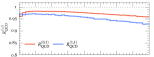
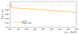
Figure 3: Transverse momentum distribution of the positively charged lepton. See the caption in Fig. 2 and the text for details.

We continue with the discussion of other observables. In Fig. 3 we show the transverse momentum distribution of the positively-charged lepton. Since at leading order the lepton transverse momentum $p_{T,\ell}$ is always smaller than $m_{\ell\ell}/2$, there is a correlation between the $p_{T,\ell}$ and the $m_{\ell\ell}$ distributions. Indeed, it follows from Fig. 3 that corrections to the transverse momentum distribution are similar to the ones to the $m_{\ell\ell}$ distribution, in that NLO EW corrections are negative and quite large, while the relative QCDxEW corrections are unusually large at low values of $p_{T,\ell}$, which give the largest contribution to the fiducial cross section. Mixed QCDxEW corrections largely follow the pattern of the NLO EW corrections. Nevertheless, the impact of the QCDxEW corrections does become slightly more important at higher values of $p_{T,\ell}$, amounting to around -3% on top of the NLO QCD and EW result at $p_{T,\ell}=500\,\text{GeV}$.

Figure 4: Distributions of the rapidity of the dilepton system and the cosine of the Collins-Soper angle. See the caption in Fig. 2 and the text for details.

Another interesting class of observables are rapidity and angular distributions. In left panes of Fig. 4 we show the rapidity of the dilepton system. We observe that both the NLO EW corrections and the mixed QCDxEW corrections are fairly flat over the considered rapidity range and amount to ${\cal O}(-3\%)$ and ${\cal O}(-1\%)$, respectively. As the fiducial cross sections are dominated by low values of $m_{\ell\ell}\approx 200$ GeV, the corrections that we see in the rapidity distribution correspond to those shown in Table 1.

Angular distributions can be used to analyze the structure of the currents that facilitate the transition from quarks to leptons both within and beyond the Standard Model. Although these angular distributions can be computed in full generality, it is simpler to discuss an integrated quantity – the forward-backward asymmetry of a lepton relative to the direction of an incoming quark. A convenient variable that allows one to study such an asymmetry is the Collins-Soper angle Collins:1977iv , defined as follows

$$\cos\theta^{*}=\frac{p_{\ell^{-}}^{+}p^{-}_{\ell^{+}}-p_{\ell^{-}}^{-}p^{+}_{\ell^{+}}}{m_{\ell\ell}\,\sqrt{m^{2}_{\ell\ell}+p_{\ell\ell,\perp}^{2}}}\times{\rm sgn}(p_{\ell\ell,z})\;.$$ (85)

In Eq. (85), $p_{i}^{\pm}=E_{i}\pm p_{z,i}$ and $p_{\ell\ell}=p_{\ell^{-}}+p_{\ell^{+}}$. We show the $\cos\theta^{*}$ distribution for events in the fiducial volume Eq. (75) in the right panel of Fig. 4. Similar to the dilepton rapidity distribution, both the NLO EW and mixed QCDxEW corrections to the Collins-Soper angle are fairly flat and are comparable to corrections to the fiducial cross section, cf. Table 1.

It is clear from Fig. 4 that the distribution of the Collins-Soper angle is not symmetric and that there are more events with $\cos\theta^{*}>0$ than with $\cos\theta^{*}<0$. To quantify this effect, we consider the forward-backward asymmetry

$$A_{\rm FB}=\frac{\sigma_{F}-\sigma_{B}}{\sigma_{F}+\sigma_{B}},$$ (86)

where

$$\sigma_{F}=\int\limits_{0}^{1}{\rm d}\cos\theta^{*}\;\frac{{\rm d}\sigma(pp\to\ell^{-}\ell^{+})}{{\rm d}\cos\theta^{*}},\;\;\;\;\;\sigma_{B}=\int\limits_{-1}^{0}{\rm d}\cos\theta^{*}\;\frac{{\rm d}\sigma(pp\to\ell^{-}\ell^{+})}{{\rm d}\cos\theta^{*}}.$$ (87)

We calculate the forward-backward asymmetry for the fiducial phase space defined in Eq. (75) including all corrections computed in this paper and find

$$A_{\rm FB}=0.1580^{+0.15\%}_{-0.07\%}\;,$$ (88)

where the uncertainties are estimated from a simultaneous scale and input-scheme variations as described above. Omitting the mixed QCDxEW corrections changes the prediction in Eq. (88) by about 2 per mille which is again comparable with the uncertainty on the central value.

It is well-known that the forward-backward asymmetry increases with the invariant mass of dileptons. For this reason, it is instructive to study the forward-backward asymmetry and mixed QCD-electroweak corrections to it in the four $m_{\ell\ell}$ windows defined in Eq. (79). The results are shown in Table 3. There we display predictions for the forward-backward asymmetry that include all corrections considered in this paper ($A_{\rm FB}$) as well as the prediction for the forward-backward asymmetry without the mixed QCDxEW correction ($\tilde{A}_{\rm FB}$). We observe that the mixed QCDxEW corrections impact the value of $A_{\rm FB}$ below the percent level in the lower invariant mass windows, and reach $-1.3\%$ at high $m_{\ell\ell}$. Such percent-level shifts above $m_{\ell\ell}\sim\text{TeV}$ should become observable at the high-luminosity LHC, provided that systematic uncertainties can be controlled.

	$\tilde{A}_{\rm FB}$	$A_{\rm FB}$
$\Phi^{(1)}$	$0.1442^{+0.05\%}_{-0.31\%}$	$0.1440^{+0.11\%}_{-0.09\%}$
$\Phi^{(2)}$	$0.1852^{+0.08\%}_{-0.40\%}$	$0.1847^{+0.10\%}_{-0.19\%}$
$\Phi^{(3)}$	$0.2401^{+0.13\%}_{-0.64\%}$	$0.2388^{+0.06\%}_{-0.47\%}$
$\Phi^{(4)}$	$0.3070^{+0.49\%}_{-1.5\%}$	$0.3031^{+0.19\%}_{-1.2\%}$

Table 3: Forward-backward asymmetry in the invariant mass windows specified through Eq. (79). We label as $\tilde{A}_{\rm FB}$ the predictions including the LO contribution and higher order corrections from NLO-QCD, NLO-EW and NNLO-QCD, whereas $A_{\rm FB}$ further includes the mixed QCDxEW correction computed here.

5 Conclusions

We presented a computation of mixed QCD-electroweak corrections to the production of dilepton pairs in proton-proton collisions, $pp\to\ell^{-}\ell^{+}$, focusing on the high-invariant mass region. We have used the two-loop amplitudes computed in Ref. Heller:2020owb and the nested soft-collinear subtraction scheme Caola:2017dug to extract and regulate the real-emission contributions. Our results are fully differential with respect to the kinematics of resolved final-state particles and can be used to compute any infrared safe observable.

We applied our result to the study of high-mass dilepton production at the 13.6  TeV LHC. We presented results for fiducial cross sections and distributions defined by kinematic cuts applied to final-state leptons in typical experimental analyses. We have selected the high-mass region by requiring that the dilepton invariant mass is larger than $200\leavevmode\nobreak\ {\rm GeV}$. With these cuts, the mixed QCDxEW corrections amount to about $-1\%$ of the LO cross section. They are therefore larger than what could have been expected based on the magnitudes of the coupling constants. In fact, in this setup they are larger than the NNLO QCD ones. The remaining uncertainty coming from scale and input-scheme variation is reduced to the sub-percent level.

For even higher invariant masses, above $1\leavevmode\nobreak\ {\rm TeV}$, the mixed corrections become even larger and appear to be driven by Sudakov logarithms. For this reason, the exact mixed QCDxEW corrections can be reliably approximated by a product of NLO QCD and EW contributions. We have checked that this factorized approximation reproduces the size of mixed corrections at $m_{\ell\ell}\sim 1\leavevmode\nobreak\ {\rm TeV}$ to within thirty percent and the accuracy of this approximation increases at higher invariant masses. We have also found that mixed QCDxEW corrections may affect the forward-backward asymmetry in the process $pp\to\ell^{-}\ell^{+}$ at the percent level for dilepton invariant masses above $1\leavevmode\nobreak\ {\rm TeV}$. This region is especially interesting for searching for New Physics effects in dilepton production. Hopefully, measurements with such a precision can be performed at the HL-LHC.

Appendix A Analytic results for mixed QCDxEW corrections for other partonic channels

A.1 The $g\bar{q}$ and $qg$ channels

In this section we present the finite partonic cross sections for the $g{\bar{q}}(gq)$ and $qg(\bar{q}g)$ channels. For the sake of simplicity we only present results for the $g{\bar{q}}(gq)$ case, results for the $qg(\bar{q}g)$ channel can be obtained with straightforward modifications that will be mentioned below. Similar to the $q{\bar{q}}$ channel (see Sec. 2.4), we isolate four different structures

$$d\hat{\sigma}_{\rm nnlo}^{g\bar{q}}=d\hat{\sigma}_{\rm bt}^{g\bar{q}}+d\hat{\sigma}_{\mathcal{O}_{\rm nlo}}^{g\bar{q}}+d\hat{\sigma}_{\rm reg}^{g\bar{q}}.$$ (89)

The regulated term reads

$$2s\cdot d\hat{\sigma}_{\rm reg}^{g\bar{q}}=\left\langle\left(I-S_{6}\right)\Omega_{g\bar{q}}F_{\rm LM}(1_{g},2_{\bar{q}},3_{\ell^{-}},4_{\ell^{+}},5_{\bar{q}},6_{\gamma})\right\rangle,$$ (90)

with

$$\begin{split}\Omega_{g\bar{q}}&=(1-C_{56,1})\,\omega^{65}\,\tilde{\theta}_{A}+(1-C_{56,1})(1-C_{56})\,\omega^{65}\,\tilde{\theta}_{B}\\ &+\,(1-C_{56,1})(1-C_{51})\,\omega^{65}\,\tilde{\theta}_{C}+(1-C_{56,1})(1-C_{56})\,\omega^{65}\,\tilde{\theta}_{D}\\ &+\,\sum_{i=2}^{4}(1-C_{51})(1-C_{6i})\,\omega^{6i},\end{split}$$ (91)

and

$$\begin{gathered}\tilde{\theta}_{A}=\theta\left(\eta_{16}<\frac{\eta_{15}}{2}\right)\leavevmode\nobreak\ \leavevmode\nobreak\ \leavevmode\nobreak\ \leavevmode\nobreak\ \tilde{\theta}_{B}=\theta\left(\frac{\eta_{15}}{2}<\eta_{16}<\eta_{15}\right)\\ \tilde{\theta}_{C}=\theta\left(\eta_{15}<\frac{\eta_{16}}{2}\right)\leavevmode\nobreak\ \leavevmode\nobreak\ \leavevmode\nobreak\ \leavevmode\nobreak\ \tilde{\theta}_{D}=\theta\left(\frac{\eta_{16}}{2}<\eta_{15}<\eta_{16}\right).\end{gathered}$$ (92)

In Eq. (91) we have also introduced the damping factors

$$\omega^{6i}=\frac{1/\eta_{6i}}{\sum_{a=2}^{5}1/\eta_{6a}}\;.$$ (93)

We note that Eq. (91) is finite, and can be evaluated numerically.

The other contributions are reported below assuming $E_{\rm max}=E_{1}=E_{2}\equiv E_{c}$. We have

$$\begin{split}2s\cdot d\hat{\sigma}_{\rm bt}^{g\bar{q}}=\,&[\alpha]\,[\alpha_{s}]\,T_{R}\,Q_{q}^{2}\,\int_{0}^{1}dz_{1}dz_{2}\,\tilde{P}^{\rm NLO}_{\bar{q}g}(z_{1},E_{c})\\ &\hskip 28.45274pt\times\Big{\langle}\frac{F_{\rm LM}(z_{1}\cdot 1_{q},z_{2}\cdot 2_{\bar{q}},3,4))}{z_{1}\,z_{2}}\Big{\rangle}\,\tilde{P}_{qq}^{\rm NLO}(z_{2},E_{c})\\ &+[\alpha_{s}]\,T_{R}\int_{0}^{1}dz\,\tilde{P}^{\rm NLO}_{\bar{q}g}(z,E_{c})\,\Big{\langle}\frac{F_{\rm LV}^{\rm(EW),\,fin}(z\cdot 1_{q},2_{\bar{q}},3,4)}{z}\Big{\rangle}\\ &+[\alpha][\alpha_{s}]\,T_{R}\int_{0}^{1}dz\,\Big{\langle}\Big{[}\tilde{P}^{\rm NLO}_{\bar{q}g}(z,E_{c})\,\Big{(}2\,Q_{e}Q_{q}\,G^{(1,2)}_{eq}\\ &\hskip 28.45274pt-\log\Big{(}\frac{s_{13}}{s_{14}}\Big{)}\log(z)+Q_{e}^{2}\,G_{e^{2}}\Big{)}+Q_{q}^{2}\,P_{{\bar{q}}g}^{\rm NNLO}(z,E_{c})\Big{]}\;\\ &\hskip 28.45274pt\times\;\frac{F_{\rm LM}(z\cdot 1_{q},2_{\bar{q}},3,4)}{z}\Big{\rangle}\;,\end{split}$$ (94)

where $P_{{\bar{q}}g}^{\rm NNLO}(z,E_{c})$ is reported in Eq. (B). The $\mathcal{O}_{\rm nlo}$ term reads

$$2s\cdot d\hat{\sigma}_{\mathcal{O}_{\rm nlo}}^{g\bar{q}}=\, \Big{\langle}\mathcal{O}^{{\bar{q}}}_{\rm nlo}\;F_{\rm LV}^{\rm(EW),\,fin}(1_{g},2_{\bar{q}},3,4|5_{\bar{q}})\Big{\rangle}$$

$$+\,[\alpha]\Big{\langle}\mathcal{O}^{{\bar{q}}}_{\rm nlo}\,\bigg{[}Q_{q}^{2}\left(G^{(5,2)}_{q^{2}}-\Big{(}\frac{3}{2}-2\log\Big{(}\frac{E_{5}}{E_{c}}\Big{)}\Big{)}\,\log\Big{(}\frac{\eta_{51}}{1-\eta_{51}}\Big{)}\right)$$

$$+\,Q_{e}^{2}\;G_{e^{2}}+2\,Q_{e}Q_{q}\left(G^{(5,2)}_{eq}-\log\Big{(}\frac{E_{5}}{E_{c}}\Big{)}\log\Big{(}\frac{s_{35}}{s_{45}}\Big{)}\right)\bigg{]}$$

$$\hskip 99.58464pt\times F_{\rm LM}(1_{g},2_{\bar{q}},3,4|5_{\bar{q}})\Big{\rangle}$$ (95)

$$+\,[\alpha]\,Q_{q}^{2}\int_{0}^{1}dz\,\tilde{P}_{qq}^{\rm NLO}(z,E_{c})\,\Big{\langle}\mathcal{O}^{\bar{q}}_{\rm nlo}\,\frac{F_{\rm LM}(1_{g},z\cdot 2_{\bar{q}},3,4|5_{\bar{q}})}{z}\Big{\rangle}$$

$$+[\alpha_{s}]\,T_{R}\int_{0}^{1}dz\,\Big{\langle}\mathcal{O}^{\gamma}_{\rm nlo}\,\Big{[}\tilde{P}^{\rm NLO}_{\bar{q}g}(z,E_{c})+\tilde{\omega}_{5\parallel 1}^{65}\,\log\Big{(}\frac{\eta_{16}}{2}\Big{)}\,\bar{P}_{{\bar{q}}g}^{\rm AP,0}(z)\Big{]}$$

$$\hskip 99.58464pt\times\,\frac{F_{\rm LM}(z\cdot 1_{q},2_{\bar{q}},3,4|6_{\gamma})}{z}\Big{\rangle}\;.$$

Here, $\mathcal{O}^{{\bar{q}}}_{\rm nlo}=1-C_{15}$, $\mathcal{O}^{\gamma}_{\rm nlo}$ is defined in Eq. (17) and $\tilde{\omega}_{5\parallel 1}^{65}=C_{51}\,\omega^{65}$. The relevant splitting functions are

$$\begin{split}&\tilde{P}^{\rm NLO}_{\bar{q}g}(z,E_{c})=2\bar{P}_{{\bar{q}}g}^{\rm AP,0}(z)\log(1-z)+2z(1-z)+\bar{P}_{{\bar{q}}g}^{\rm AP,0}(z)\log\Big{(}\frac{4E_{c}^{2}}{\mu^{2}}\Big{)}\;,\\ &\bar{P}_{{\bar{q}}g}^{\rm AP,0}(z)=(1-z)^{2}+z^{2}\,.\end{split}$$ (96)

Finally, we have

$$\begin{split}G^{(i,j)}_{q^{2}}=&\frac{13}{2}-\pi^{2}+2{\rm Li}_{2}\big{(}1-\eta_{ij}\big{)}+\log^{2}\Big{(}\frac{E_{i}}{E_{c}}\Big{)}+\frac{3}{2}\log\Big{(}\frac{E_{c}^{2}}{\mu^{2}}\Big{)}\\ &+\bigg{(}3-2\log\Big{(}\frac{E_{i}}{E_{c}}\Big{)}\bigg{)}\,\log\big{(}4\,\eta_{ij}\big{)}\;.\end{split}$$ (97)

The functions $G_{e^{2}}$ and $G_{eq}$ have already been defined for the $q{\bar{q}}$ channel in Eq. (67).

In Eqs. (94)–(A.1) we define $Q_{q}$ as minus the electric charge of the initial state anti-quark, i.e. $Q_{q}=\{-1/3,2/3\}$ for the down and up quarks respectively. In order to obtain the results for the $gq$ channel it is sufficient to flip the sign of the quark electric charge, i.e. $Q_{q}\rightarrow-Q_{q}$, and apply the replacement $\bar{q}\to q$ inside the relevant matrix elements. As for the $qg$ channel one can start from Eqs. (94)–(A.1) and follow a simple set of rules. In practice, for Eq. (94) it is enough to consider

$$F_{\rm LM(V)}(z\cdot 1_{q},2_{\bar{q}})\to F_{\rm LM(V)}(1_{q},z\cdot 2_{\bar{q}}),\quad\tilde{P}^{\mathrm{NLO}}_{ij}(z_{1},E_{c})\leftrightarrow\tilde{P}^{\mathrm{NLO}}_{ij}(z_{2},E_{c}),\quad s_{1k}\to s_{2k},$$

whereas for Eq. (A.1), one has

$$F_{\rm LM(V)}(z\cdot 1_{q},2_{\bar{q}})\to F_{\rm LM(V)}(1_{q},z\cdot 2_{\bar{q}}),\quad F_{\rm LM(V)}(1_{g},z\cdot 2_{\bar{q}})\to F_{\rm LM(V)}(z\cdot 1_{q},2_{g}),\quad$$

$$G^{(5,2)}_{q^{2}}\to G^{(5,1)}_{q^{2}}\,,\quad\eta_{k1}\to\eta_{k2}\,,\quad\tilde{\omega}_{5\parallel 1}^{65}\to\tilde{\omega}_{5\parallel 2}^{65}\,.$$

A.2 The $\gamma\bar{q}$ and $q\gamma$ channels

The partonic channels induced by photon-(anti)quark scattering receive contributions from two different configurations: one where an intermediate $Z/\gamma$ decays into leptons, and one where the leptons are produced directly from the initial state photon. The IR structure of the first configuration is similar to the $gq({\bar{q}})$ case. We then expect the final formulas to be similar to Eqs. (94)–(A.1), upon setting $Q_{e}\rightarrow 0$, $T_{R}\rightarrow N_{c}C_{F}$, and replacing the gluon with the photon in all the relevant matrix elements. The contribution of the direct lepton production results in additional terms proportional to Born- and NLO-level boosted matrix elements. For the sake of simplicity we focus on the $\gamma(1){\bar{q}}(2)\rightarrow\ell^{-}\ell^{+}g(5){\bar{q}}(6)$ process. In order to disentangle all the relevant collinear singularities, we introduce the partition

$$1=\omega^{51,61}+\omega^{52,62}+\omega^{52,61}+\omega^{51,62}\,,$$ (98)

where the definition of the $\omega^{5i,6j}$ functions can be found in Ref. Caola:2017dug . We then write the final result as

$$d\hat{\sigma}_{\rm nnlo}^{\gamma\bar{q}}=d\hat{\sigma}_{\rm bt}^{\gamma\bar{q}}+d\hat{\sigma}_{\mathcal{O}_{\rm nlo}}^{\gamma\bar{q}}+d\hat{\sigma}_{\rm reg}^{\gamma\bar{q}}\,.$$ (99)

The regulated contribution reads

$$2s\cdot d\hat{\sigma}_{\rm reg}^{\gamma\bar{q}}=\left\langle(1-S_{5})\Omega_{\gamma{\bar{q}}}F_{\rm LM}(1_{\gamma},2_{\bar{q}},3_{\ell^{-}},4_{\ell^{+}},5_{g},6_{\bar{q}})\right\rangle,$$ (100)

with

$$\begin{split}\Omega_{\,\gamma\bar{q}}&=(1-C_{56,1})(1-C_{61})\,\omega^{51,61}\,\tilde{\theta}_{A}+(1-C_{56,1})(1-C_{56})\,\omega^{51,61}\,\tilde{\theta}_{B}\\ &+\,(1-C_{56,1})\,\omega^{51,61}\,\tilde{\theta}_{C}+(1-C_{56,1})(1-C_{56})\,\omega^{51,61}\,\tilde{\theta}_{D}\\ &+\,(1-C_{56,2})\,\omega^{52,62}\,\tilde{\theta}_{A}+(1-C_{56,2})(1-C_{56})\,\omega^{52,62}\,\tilde{\theta}_{B}\\ &+\,(1-C_{56,2})(1-C_{52})\,\omega^{52,62}\,\tilde{\theta}_{C}+(1-C_{56,2})(1-C_{56})\,\omega^{52,62}\,\tilde{\theta}_{D}\\ &+\omega^{51,62}+(1-C_{52})(1-C_{61})\omega^{52,61}\;,\end{split}$$ (101)

and $\tilde{\theta}_{I}$ defined in Eq. (92).

The boost contribution reads

$$\begin{split}2s\,\cdot\,&d\hat{\sigma}_{\rm bt}^{\gamma\bar{q}}=\,[\alpha]\,[\alpha_{s}]\,Q_{q}^{2}\,N_{c}\,C_{F}\,\int_{0}^{1}dz_{1}dz_{2}\,\tilde{P}^{\rm NLO}_{\bar{q}g}(z_{1},E_{c})\\ &\hskip 56.9055pt\times\Big{\langle}\frac{F_{\rm LM}(z_{1}\cdot 1_{q},z_{2}\cdot 2_{\bar{q}},3,4))}{z_{1}\,z_{2}}\Big{\rangle}\,\tilde{P}_{qq}^{\rm NLO}(z_{2},E_{c})\\ &+[\alpha]\,Q_{q}^{2}\,N_{c}\,\int_{0}^{1}dz\,\tilde{P}^{\rm NLO}_{\bar{q}g}(z,E_{c})\,\Big{\langle}\frac{F_{\rm LV}^{\rm(QCD),\,fin}(z\cdot 1_{q},2_{\bar{q}},3,4)}{z}\Big{\rangle}\\ &+\,[\alpha]\,[\alpha_{s}]\,Q_{q}^{2}\,C_{F}\int_{0}^{1}dz\,\bigg{[}N_{c}\,P^{{\rm NNLO},\,s}_{\gamma\bar{q}}(z,E_{c})\Big{\langle}\frac{F_{LM}(z\cdot 1_{q},2_{\bar{q}},3,4)}{z}\Big{\rangle}\\ &\hskip 56.9055pt+\,P^{{\rm NNLO},\,t}_{\gamma\bar{q}}(z,E_{c})\Big{\langle}\frac{F_{\rm LM}(1_{\gamma},z\cdot 2_{\gamma},3,4)}{z}\Big{\rangle}\bigg{]}\;,\end{split}$$ (102)

where the first term in squared brackets is the same as for the $g{\bar{q}}$ channel, i.e. $P^{{\rm NNLO},\,s}_{\gamma\bar{q}}=P_{{\bar{q}}g}^{\rm NNLO}$, while $P^{{\rm NNLO},\,t}_{\gamma\bar{q}}$ stems from the direct lepton production and is reported in Eq. (B). The $\mathcal{O}_{\rm nlo}$ contributions is

$$\begin{split}2s\,\cdot\,&d\hat{\sigma}_{\mathcal{O}_{\rm nlo}}^{\gamma\bar{q}}=\Big{\langle}\mathcal{O}_{\rm nlo}^{\bar{q}}\;F_{\rm LV}^{\rm(QCD),\,fin}(1_{\gamma},2_{\bar{q}},3,4|6_{\bar{q}})\Big{\rangle}\\ &+[\alpha_{s}]\,C_{F}\;\Big{\langle}\mathcal{O}_{\rm nlo}^{\bar{q}}\;\Big{[}G^{(6,2)}_{q^{2}}-\sum_{i=1}^{2}\bigg{(}\frac{3}{2}-2\log\Big{(}\frac{E_{6}}{E_{c}}\Big{)}\bigg{)}\,\log\Big{(}\frac{\eta_{i6}}{1-\eta_{i6}}\Big{)}\,\tilde{\omega}^{5i,6i}_{5\parallel 6}\Big{]}\\ &\hskip 71.13188pt\;\times F_{\rm LM}(1_{\gamma},2_{\bar{q}},3,4|6_{\bar{q}})\Big{\rangle}\\ &+[\alpha]\,Q_{q}^{2}\,N_{c}\int_{0}^{1}dz\,\Big{\langle}\mathcal{O}_{\rm nlo}^{g}\;\Big{[}\tilde{P}^{\rm NLO}_{\bar{q}g}(z,E_{c})\\ &\hskip 71.13188pt+\,\tilde{\omega}^{51,61}_{6\parallel 1}\,\log\Big{(}\frac{\eta_{51}}{2}\Big{)}\;\bar{P}_{g{\bar{q}}}^{\rm AP,0}(z)\Big{]}\,\frac{F_{\rm LM}(z\cdot 1_{q},2_{\bar{q}},3,4|5_{g})}{z}\Big{\rangle}\\ &+[\alpha_{s}]\,C_{F}\int_{0}^{1}dz\,\Big{\langle}\mathcal{O}_{\rm nlo}^{{\bar{q}}}\;\Big{[}\tilde{P}_{qq}^{\rm NLO}(z,E_{c})\\ &\hskip 71.13188pt+\,\tilde{\omega}^{52,62}_{5\parallel 2}\;\log\Big{(}\frac{\eta_{62}}{2}\Big{)}\,\bar{P}_{qq,\rm R}^{\rm AP,0}(z)\Big{]}\frac{F_{\rm LM}(1_{\gamma},z\cdot 2_{\bar{q}},3,4|6_{\bar{q}})}{z}\Big{\rangle}\;,\end{split}$$ (103)

where we have introduced $\tilde{P}^{\rm NLO}_{\bar{q}g}$ and $\bar{P}_{{\bar{q}}g}^{\rm AP,0}$ in Eq. (96), $G^{(6,2)}_{q^{2}}$ in Eq. (97), and $\bar{P}_{qq,\,\rm R}^{\rm AP,0}$ in Eq. (66). One can obtain results for the $\gamma q$, $q\gamma$ and ${\bar{q}}\gamma$ channels following the discussion at the end of Sec. A.1.

A.3 The $\gamma g$ and $g\gamma$ channels

The NNLO corrections to the cross sections in the $\gamma g$ and $g\gamma$ partonic channels are affected only by collinear singularities that cancel upon combining real corrections and PDF renormalization. In order to regularize real radiations, we introduce the same phase space partition as in Eq. (98). The subtraction then proceeds as usual. The final result for the $\gamma g$ channel can be cast in the following form

$$d\hat{\sigma}_{\rm nnlo}^{\gamma g}=d\hat{\sigma}_{\rm bt}^{\gamma g}+d\hat{\sigma}_{\mathcal{O}_{\rm nlo}}^{\gamma g}+d\hat{\sigma}_{\rm reg}^{\gamma g}\,.$$ (104)

The regulated part reads

$$2s\cdot d\hat{\sigma}_{\rm reg}^{\gamma g}=\left\langle\Omega_{\gamma g}F_{\rm LM}(1_{\gamma},2_{g},3_{\ell^{-}},4_{\ell^{-}},5_{q},6_{\bar{q}})\right\rangle,$$ (105)

where

$$\begin{split}\Omega_{\gamma g}&=(1-C_{51}-C_{61})\,\omega^{51,61}\\ &+\,(1-C_{56,2})\,(1-C_{62})\,\omega^{52,62}\,\tilde{\theta}_{A}+(1-C_{56,2})(1-C_{52})\,\omega^{52,62}\,\tilde{\theta}_{C}\\ &+(1-C_{62})\,(1-C_{51})\,\omega^{51,62}+(1-C_{61})\,(1-C_{52})\,\omega^{52,61}\\ &+\,(1-C_{56,2})\,\omega^{52,62}\,\tilde{\theta}_{B}+(1-C_{56,2})\,\omega^{52,62}\,\tilde{\theta}_{D}\;,\end{split}$$ (106)

with $w^{5i,6j}$ and $\tilde{\theta}$ as in Sec. A.2.

The other relevant definitions are

$$\begin{split}2s\,\cdot\,&d\hat{\sigma}_{\rm bt}^{\gamma g}=[\alpha]\,[\alpha_{s}]\,Q_{q}^{2}\,T_{R}\,N_{c}\,\int_{0}^{1}dz_{1}dz_{2}\,\tilde{P}^{\rm NLO}_{\bar{q}g}(z_{1},E_{c})\,\tilde{P}_{\bar{q}g}^{\rm NLO}(z_{2},E_{c})\\ &\quad\times\bigg{[}\Big{\langle}\frac{F_{\rm LM}(z_{1}\cdot 1_{q},z_{2}\cdot 2_{\bar{q}},3,4))}{z_{1}\,z_{2}}\Big{\rangle}+\Big{\langle}\frac{F_{\rm LM}(z_{1}\cdot 1_{{\bar{q}}},z_{2}\cdot 2_{q},3,4))}{z_{1}\,z_{2}}\Big{\rangle}\bigg{]}\\ &+\,[\alpha]\,[\alpha_{s}]\,Q_{q}^{2}\,T_{R}\,\int_{0}^{1}dz\,P^{\rm NNLO}_{\gamma g}(z,E_{c})\,\Big{\langle}\frac{F_{\rm LM}(1_{\gamma},z\cdot 2_{\gamma},3,4)}{z}\Big{\rangle}\;,\\ 2s\,\cdot\,&d\hat{\sigma}_{\mathcal{O}_{\rm nlo}}^{\gamma g}=[\alpha]\,Q_{q}^{2}\,N_{c}\int_{0}^{1}dz\,\tilde{P}^{\rm NLO}_{\bar{q}g}(z,E_{c})\\ &\qquad\times\,\bigg{[}\Big{\langle}\mathcal{O}_{\rm nlo}^{q}\;\frac{F_{\rm LM}(z\cdot 1_{q},2_{g},3,4|5_{q})}{z}\Big{\rangle}+\Big{\langle}\mathcal{O}_{\rm nlo}^{{\bar{q}}}\;\frac{F_{\rm LM}(z\cdot 1_{{\bar{q}}},2_{g},3,4|6_{\bar{q}})}{z}\Big{\rangle}\bigg{]}\\ &\quad+\,[\alpha_{s}]\,T_{R}\int_{0}^{1}dz\,\Big{\langle}\mathcal{O}_{\rm nlo}^{{\bar{q}}}\;\Big{[}\tilde{P}^{\rm NLO}_{\bar{q}g}(z,E_{c})+\\ &\hskip 71.13188pt+\,\tilde{\omega}^{52,62}_{6\parallel 2}\,\log\Big{(}\frac{\eta_{52}}{2}\Big{)}\;\bar{P}_{g{\bar{q}}}^{\rm AP,0}(z)\Big{]}\,\frac{F_{\rm LM}(1_{\gamma},z\cdot 2_{q},3,4|5_{q})}{z}\Big{\rangle}\\ &\quad+\,[\alpha_{s}]\,T_{R}\int_{0}^{1}dz\,\Big{\langle}\mathcal{O}_{\rm nlo}^{{\bar{q}}}\;\Big{[}\tilde{P}^{\rm NLO}_{\bar{q}g}(z,E_{c})+\\ &\hskip 71.13188pt+\,\tilde{\omega}^{52,62}_{5\parallel 2}\,\log\Big{(}\frac{\eta_{62}}{2}\Big{)}\;\bar{P}_{g{\bar{q}}}^{\rm AP,0}(z)\Big{]}\,\frac{F_{\rm LM}(1_{\gamma},z\cdot 2_{\bar{q}},3,4|6_{\bar{q}})}{z}\Big{\rangle}\;,\end{split}$$ (107)

where $P^{\rm NNLO}_{\gamma g}(z,E_{c})$ is defined in Eq. (B). One can deduce the result for the $g\gamma$ channel by taking Eq. (107) and swapping the indices 1 and 2.

A.4 The $q{\bar{q}}\rightarrow\ell^{-}\ell^{+}q{\bar{q}}$ and $qq$ channels

The $q{\bar{q}}\rightarrow\ell^{-}\ell^{+}q{\bar{q}}$ and $qq\rightarrow\ell^{-}\ell^{+}qq$ partonic processes are only affected by triple collinear singularities, that are compensated by the PDF renormalization contribution. The phase space partition that we choose for both channels reads

$$1=w^{51,61}+w^{52,62}=\frac{\eta_{52}}{\eta_{51}+\eta_{52}}+\frac{\eta_{51}}{\eta_{51}+\eta_{52}}\,.$$ (108)

For both channels we write

$$\begin{split}d\hat{\sigma}_{\rm nnlo}^{qq}=d\hat{\sigma}_{\rm bt}^{qq}+d\hat{\sigma}_{\rm reg}^{qq},\leavevmode\nobreak\ \leavevmode\nobreak\ \leavevmode\nobreak\ \leavevmode\nobreak\ \leavevmode\nobreak\ \leavevmode\nobreak\ \leavevmode\nobreak\ \leavevmode\nobreak\ \leavevmode\nobreak\ \leavevmode\nobreak\ \leavevmode\nobreak\ \leavevmode\nobreak\ d\hat{\sigma}_{{\rm nnlo},q\bar{q}}^{q\bar{q}}=d\hat{\sigma}_{{\rm bt},q\bar{q}}^{q\bar{q}}+d\hat{\sigma}_{{\rm reg},q\bar{q}}^{q\bar{q}}\,.\end{split}$$ (109)

In the $q\bar{q}\to\ell^{-}\ell^{+}q\bar{q}$ channel we have

$$2s\cdot d\hat{\sigma}_{{\rm reg},q\bar{q}}^{q\bar{q}}=\left\langle\sum_{i=1}^{2}(1-C_{56,i})\omega^{5i,6i}F_{\rm LM}(1_{q},2_{\bar{q}},3_{\ell^{-}},4_{\ell^{+}},5_{q},6_{\bar{q}})\right\rangle\,,$$ (110)

and

$$\begin{split}2s\cdot d\hat{\sigma}_{{\rm bt},q\bar{q}}^{q\bar{q}}=\,&[\alpha]\,[\alpha_{s}]\,2\,Q_{q}^{2}\,C_{F}\,\int_{0}^{1}dz\,P^{\rm NNLO}_{q\bar{q}\rightarrow q\bar{q}}(z,E_{c})\\ &\times\,\bigg{[}\Big{\langle}\frac{F_{\rm LM}(z\cdot 1_{q},2_{{\bar{q}}},3,4)}{z}\Big{\rangle}+\Big{\langle}\frac{F_{\rm LM}(1_{q},z\cdot 2_{\bar{q}},3,4)}{z}\Big{\rangle}\bigg{]}\;,\end{split}$$ (111)

with $P^{\rm NNLO}_{q\bar{q}\to q\bar{q}}$ defined in Eq. (B).

For the $qq\to\ell^{-}\ell^{+}qq$ channel, we have instead

$$2s\cdot d\hat{\sigma}_{{\rm reg}}^{qq}=\left\langle\big{[}(1-C_{56,1})\omega^{51,61}+\omega^{52,62}\big{]}F_{\rm LM}(1_{q},2_{q},3_{\ell^{-}},4_{\ell^{+}},5_{q},6_{q})\right\rangle\,,$$ (112)

and

$$\begin{split}2s\cdot d\hat{\sigma}_{\rm bt}^{qq}=\,&[\alpha]\,[\alpha_{s}]\,2\,Q_{q}^{2}\,C_{F}\,\int_{0}^{1}dz\,P^{\rm NNLO}_{qq\rightarrow qq}(z,E_{c})\Big{\langle}\frac{F_{\rm LM}(z\cdot 1_{{\bar{q}}},2_{q},3,4)}{z}\Big{\rangle}\,,\end{split}$$ (113)

with $P^{\rm NNLO}_{qq\rightarrow qq}$ given in Eq. (B).

Appendix B Splitting functions

In this section we collect the splitting functions that we have introduced in the main text. We begin by defining the functions that describe the hard-collinear integrated counterterm. For initial state and final state emission we have, respectively,

$$\begin{split}P_{qq}^{\rm NLO}(z,L_{i})=\,&\bigg{[}(1-z)^{-2\epsilon}P_{qq}(z)+\frac{1}{\epsilon}\,e^{-2\epsilon L_{i}}\,\delta(1-z)\bigg{]}\;,\\ P_{qq}^{\rm NLO}(L_{i})=\,&\gamma_{ee}^{22}+\frac{1}{\epsilon}\bigg{(}1-e^{-2\epsilon L_{i}}\bigg{)}\;,\end{split}$$ (114)

where

$$\gamma_{ee}^{22}=-\int_{0}^{1}dz\;\bigg{\{}\big{[}z(1-z)\big{]}^{-2\epsilon}P_{qq}\big{(}z\big{)}-2\,\frac{(1-z)^{-2\epsilon}}{1-z}\bigg{\}}\;.$$ (115)

The LO Altarelli-Parisi splitting functions we have used are

$$\begin{split}\bar{P}_{qq}^{\rm AP,0}(z)=\,&2\mathcal{D}_{0}(z)-(1+z)+\frac{3}{2}\,\delta(1-z)\,,\\ \bar{P}_{\bar{q}g}^{\rm AP,0}(z)=\,&(1-z)^{2}+z^{2}\,,\\ \bar{P}_{q\gamma}^{\rm AP,0}(z)=\,&\frac{1+(1-z)^{2}}{z}\,,\end{split}$$ (116)

where the regular part of $\bar{P}_{qq}^{\rm AP,0}$ is equal to

$$\bar{P}_{qq,R}^{\rm AP,0}(z)=2\mathcal{D}_{0}(z)-(1+z)\,.$$ (117)

In order to describe the single-collinear limits of the $q{\bar{q}}\rightarrow\ell^{-}\ell^{+}(g\gamma)$ we compute

$$\begin{split}\big{[}\bar{P}_{qq}^{\rm AP,0}\otimes\bar{P}_{qq}^{\rm AP,0}\big{]}(z)=\,&6\mathcal{D}_{0}(z)+8\mathcal{D}_{1}(z)+\Big{(}\frac{9}{4}-\frac{2\pi^{2}}{3}\Big{)}\,\delta(1-z)-\frac{\big{(}3z^{2}+1\big{)}\log(z)}{1-z}\\ &-z-4(z+1)\,\log(1-z)-5\,.\end{split}$$ (118)

At one-loop level, the Altarelli-Parisi splitting function for process $q\rightarrow qg$ reads

$$\begin{split}\bar{P}_{qq}^{\rm AP,1}(z)=&3-2z+2\left[1-\frac{1+z^{2}}{1-z}\log(1-z)\right]\log z+\frac{1+3z^{2}}{2(1-z)}\log^{2}z\\ &+\frac{2(1+z^{2})}{1-z}\,{\rm Li}_{2}(1-z)+\delta(1-z)\left(\frac{3}{8}-\frac{\pi^{2}}{2}+6\zeta_{3}\right).\end{split}$$ (119)

The real-virtual splitting is

$$\begin{split}\mathcal{P}_{qq}^{{\rm loop},\,RV}(z)=\,&\frac{1}{\epsilon}\frac{1+z^{2}}{1-z}\,\log z\\ &-\frac{1+z^{2}}{1-z}\Big{(}{\rm Li}_{2}(1-z)+3\log(1-z)\log z\Big{)}-\frac{z}{2}-(1-z)\log z\\ &-\bigg{[}\frac{1}{2}\Big{(}1+z-3z\log(1-z)\Big{)}-(1-z)\Big{(}3\log(1-z)\,\log z\\ &\quad+{\rm Li}_{2}(1-z)\Big{)}-\frac{1}{2}\,\frac{1+z^{2}}{1-z}\Big{(}9\log^{2}(1-z)\,\log z\\ &\qquad+6\log(1-z)\,{\rm Li}_{2}(1-z)-2{\rm Li}_{3}(1-z)\Big{)}\bigg{]}\epsilon+\mathcal{O}(\epsilon^{2})\,.\end{split}$$ (120)

To express the finite contributions to the $q{\bar{q}}\rightarrow\ell^{-}\ell^{+}(\gamma g)$ channel partonic cross sections we have introduced the NLO splitting function

$$\begin{split}\tilde{P}_{qq}^{\rm NLO}(z,E_{c})&=\,4\mathcal{D}_{1}(z)-2(1+z)\log(1-z)+(1-z)\\ &+2\log\Big{(}\frac{2E_{c}}{\mu}\Big{)}\big{(}2\mathcal{D}_{0}(z)-(1+z)\big{)}\;.\end{split}$$ (121)

The finite contributions to the different partonic channels depend on collinear functions that multiply boosted matrix elements. For the $q{\bar{q}}\rightarrow\ell^{-}\ell^{+}(\gamma g)$ channel we have

$$P_{qq}^{\rm NNLO}(z,E_{c})\, =\mathcal{D}_{0}(z)\Big{[}48\log^{2}\Big{(}\frac{2E_{c}}{\mu}\Big{)}-\frac{16}{3}\log^{3}(z)+32\zeta_{3}\Big{]}+\log\Big{(}\frac{2E_{c}}{\mu}\Big{)}\Big{[}48\mathcal{D}_{1}(z)$$

$$-8(z+1)\text{Li}_{2}(z)-\frac{8(z^{2}+1)\text{Li}_{2}(1-z)}{z-1}-20z+\frac{4}{3}\pi^{2}(z+1)+24\Big{]}$$

$$\,-16(-2\mathcal{D}_{1}(z)+z+2)\log^{2}\Big{(}\frac{2E_{c}}{\mu}\Big{)}+\mathcal{D}_{2}(z)\Big{(}48\log\Big{(}\frac{2E_{c}}{\mu}\Big{)}-16\log(z)\Big{)}$$

$$+\log^{2}(z)\Big{[}-8\mathcal{D}_{1}(z)+2(z+1)\log\Big{(}\frac{2E_{c}}{\mu}\Big{)}-z+2\Big{]}$$

$$+16\mathcal{D}_{3}(z)+\log(1-z)\Big{[}-\frac{\log(z)}{1-z}\Big{(}8(z^{2}+1)\log\Big{(}\frac{2E_{c}}{\mu}\Big{)}$$

$$-2(5z^{2}+2z+5)\Big{)}-16(z+1)\log^{2}\Big{(}\frac{2E_{c}}{\mu}\Big{)}-16(z+2)\log\Big{(}\frac{2E_{c}}{\mu}\Big{)}$$

$$-\frac{6(z^{2}+1)\text{Li}_{2}(1-z)}{z-1}-8(z+1)\text{Li}_{2}(z)-9z+\frac{4}{3}\pi^{2}(z+1)$$ (122)

$$+4(z+1)\log^{2}(z)+12\Big{]}+\log(z)\Big{[}\frac{4(3z^{2}+1)\log^{2}\Big{(}\frac{2E_{c}}{\mu}\Big{)}}{z-1}$$

$$-\frac{8(z^{2}+z+1)\log\Big{(}\frac{2E_{c}}{\mu}\Big{)}}{z-1}-\frac{4(z^{2}+1)\text{Li}_{2}(z)}{z-1}+\frac{\pi^{2}(8z^{2}+8)}{3-3z}-9z+5\Big{]}$$

$$+\log^{2}(1-z)\Big{[}-24(z+1)\log\Big{(}\frac{2E_{c}}{\mu}\Big{)}+\frac{(5z^{2}+13)\log(z)}{1-z}+4(z-1)\Big{]}$$

$$+\frac{(10-6z^{2})\text{Li}_{3}(1-z)}{z-1}+\frac{4(3z^{2}+5)\text{Li}_{3}(z)}{z-1}+(2-2z)\text{Li}_{2}(1-z)$$

$$+4(z-1)\text{Li}_{2}(z)-\frac{4(7z^{2}+1)\zeta_{3}}{z-1}+\frac{(13z^{2}+47)\log^{3}(z)}{6-6z}-\frac{10}{3}\pi^{2}(z-1)$$

$$+2(8z-9)-8(z+1)\log^{3}(1-z)\;.$$

When discussing the finite remainders for the $g\bar{q}$ and $qg$ channels we introduced

$$P_{{\bar{q}}g}^{\rm NNLO}(z,E_{c})=\, \log\Big{(}\frac{2E_{c}}{\mu}\Big{)}\bigg{[}(8z-4)\text{Li}_{2}(z)+\frac{4}{3}\pi^{2}(z-1)^{2}+z(30z-41)$$

$$\quad+\big{(}12(z-1)z+6\big{)}\log^{2}(1-z)+(1-2z)\log^{2}(z)$$

$$\quad-(8(z-2)z+2)\log(1-z)+(20(z-1)z$$

$$\quad-(8(z-1)z+4)\log(1-z)+3)\log(z)+16\bigg{]}$$

$$+\log^{2}\Big{(}\frac{2E_{c}}{\mu}\Big{)}\bigg{[}4z(3z-2)-(8z^{2}-4z+2)\log(z)$$ (123)

$$+(8(z-1)z+4)\log(1-z)+5\bigg{]}+\big{(}2(9-5z)z-9\big{)}\text{Li}_{3}(1-z)$$

$$+\big{(}2(9-7z)z-9\big{)}\text{Li}_{3}(z)-49z^{2}+\text{Li}_{2}(z)\Big{(}\big{(}2(z-1)z+1\big{)}\log(z)$$

$$-(2(z-5)z+5)\log(1-z)+3\Big{)}+\log^{3}(z)\bigg{[}\frac{7z^{2}}{3}-\frac{5z}{2}+\frac{5}{4}\bigg{]}$$

$$+\log^{2}(z)\bigg{[}z^{2}-\frac{z}{2}-\Big{(}5(z-1)z+\frac{5}{2}\Big{)}\log(1-z)-\frac{3}{8}\bigg{]}$$

$$+\log(z)\bigg{[}\frac{35z}{4}+\frac{4}{3}\pi^{2}(2(z-1)z+1)-\Big{(}(z-5)z+\frac{5}{2}\Big{)}\log^{2}(1-z)$$

$$+(14(z-1)z+6)\log(1-z)-8z^{2}+1\bigg{]}$$

$$+\log(1-z)\bigg{[}44z^{2}+\pi^{2}\Big{(}z^{2}-\frac{7z}{3}+\frac{7}{6}\Big{)}-\frac{109z}{2}+16\bigg{]}$$

$$+8(2(z-1)z+1)\zeta_{3}+(4z(4z-5)+10)\zeta_{3}+\frac{255z}{4}$$

$$+\frac{1}{12}\pi^{2}\big{(}2z(9z-13)+11\big{)}+\frac{11}{6}\big{(}2(z-1)z+1\big{)}\log^{3}(1-z)$$

$$+\big{(}(21-17z)z-7\big{)}\log^{2}(1-z)-\frac{69}{4}\;,$$

To present the results for the $\gamma\bar{q}$ and $q\gamma$ channels we have defined the function

$$P^{{\rm NNLO},\,t}_{\gamma\bar{q}}(z,E_{c})= \log\Big{(}\frac{2E_{c}}{\mu}\Big{)}\bigg{[}4(z-2)\text{Li}_{2}(z)+\pi^{2}\Big{(}-2z-\frac{8}{3z}+4\Big{)}-4z+\frac{10}{z}$$

$$\qquad\qquad+6\Big{(}z+\frac{2}{z}-2\Big{)}\log^{2}(1-z)+(2-z)\log^{2}(z)$$

$$\qquad\qquad+\Big{(}-8z-\frac{12}{z}+20\Big{)}\log(1-z)+(5z+8)\log(z)-15\bigg{]}$$

$$+\log^{2}\Big{(}\frac{2E_{c}}{\mu}\Big{)}\bigg{[}-z+\Big{(}4z+\frac{8}{z}-8\Big{)}\log(1-z)+(4-2z)\log(z)+4\bigg{]}$$

$$-(5z+8)\text{Li}_{2}(z)+4(z-2)\text{Li}_{3}(1-z)+(2z-4)\text{Li}_{3}(z)$$ (124)

$$+\Big{(}6z+\frac{16}{z}-12\Big{)}\zeta_{3}+\frac{9\pi^{2}z}{4}-\frac{29z}{4}+\frac{5\pi^{2}}{2z}-\frac{27}{z}-\frac{11\pi^{2}}{6}+\frac{73}{2}$$

$$+\frac{\log(1-z)}{6z}\bigg{[}24(z-2)z\,\text{Li}_{2}(z)-3z(3z+46)-2\pi^{2}\big{(}7(z-2)z+10\big{)}$$

$$+108\bigg{]}+\frac{13\big{(}(z-2)z+2\big{)}\log^{3}(1-z)}{6z}+\frac{1}{12}(2-z)\log^{3}(z)$$

$$+\frac{1}{4}\bigg{(}-27z-\frac{42}{z}+58\bigg{)}\log^{2}(1-z)+\Big{(}\frac{17z}{8}+\frac{5}{2}\Big{)}\log^{2}(z)$$

$$+\Big{(}\frac{1}{4}(5z-3)+2(z-2)\log^{2}(1-z)\Big{)}\log(z)\;.$$

For the $\gamma g$ and $g\gamma$ channels we need

$$P^{\rm NNLO}_{\gamma g}(z,E_{c})=\, \log(1-z)\bigg{[}-16(z+1)\text{Li}_{2}(z)-\frac{8(z-1)\big{(}4z^{2}+7z+4\big{)}}{3z}\log\Big{(}\frac{2E_{c}}{\mu}\Big{)}$$

$$\quad+\frac{4}{9z}\big{(}38z^{3}+6\pi^{2}z(z+1))+39z^{2}-57z-20\big{)}\bigg{]}$$

$$+\text{Li}_{2}(z)\bigg{[}4(3z+1)-16(z+1)\log\Big{(}\frac{2E_{c}}{\mu}\Big{)}\bigg{]}-16(z+1)\text{Li}_{3}(1-z)$$

$$-8(z+1)\text{Li}_{3}(z)-\frac{4(z-1)\big{(}4z^{2}+7z+4\big{)}}{3z}\,\log^{2}\Big{(}\frac{2E_{c}}{\mu}\Big{)}$$

$$+\frac{4}{9z}\big{(}38z^{3}+6\pi^{2}z(z+1)+39z^{2}-57z-20\big{)}\log\Big{(}\frac{2E_{c}}{\mu}\Big{)}$$ (125)

$$+\log^{2}(z)\Big{[}4(z+1)\log\Big{(}\frac{2E_{c}}{\mu}\Big{)}+\frac{1}{2}(-11z-5)\Big{]}$$

$$+\log(z)\bigg{[}8(z+1)\log^{2}\Big{(}\frac{2E_{c}}{\mu}\Big{)}-4(3z+1)\Big{(}\frac{2E_{c}}{\mu}\Big{)}+2(3z+1)$$

$$-8(z+1)\log^{2}(1-z)\bigg{]}-\frac{4(z-1)\big{(}4z^{2}+7z+4\big{)}\log^{2}(1-z)}{3z}$$

$$+8(z+1)\zeta_{3}+\frac{1}{3}(z+1)\log^{3}(z)+\frac{2}{27z}\Big{(}12\pi^{2}(z^{3}-1)-211z^{3}$$

$$-18\pi^{2}z(z+1)-420z^{2}+528z+103\Big{)}\;.$$

Finally, we report the collinear functions appearing in the final results for the $q{\bar{q}}\rightarrow\ell^{-}\ell^{+}(q{\bar{q}})$ and $qq\rightarrow\ell^{-}\ell^{+}(qq)$ channels. We define respectively

$$P^{\rm NNLO}_{q{\bar{q}}\rightarrow q{\bar{q}}}(z,E_{c})=\, \frac{1+z^{2}}{1-z}\bigg{[}\log\Big{(}\frac{2E_{c}}{\mu}\Big{)}\bigg{(}4\text{Li}_{2}(z)-2\log^{2}(z)+4\log(1-z)\log(z)-\frac{2\pi^{2}}{3}\bigg{)}$$

$$+6\text{Li}_{3}(1-z)+8\text{Li}_{3}(-z)+9\text{Li}_{3}(z)+4\text{Li}_{2}(z)\log(1-z)$$

$$-\log(z)\bigg{(}4\text{Li}_{2}(-z)+3\text{Li}_{2}(z)-4\log^{2}(1-z)+\frac{2\pi^{2}}{3}\bigg{)}$$

$$-\frac{7}{6}\log^{3}(z)-\frac{1}{2}\log(1-z)\log^{2}(z)-\frac{2}{3}\pi^{2}\log(1-z)\bigg{]}$$ (126)

$$+\bigg{(}\frac{(10-4z^{2})\log(z)}{z-1}+2(7z-8)\bigg{)}\log\Big{(}\frac{2E_{c}}{\mu}\Big{)}+\frac{(z^{2}+6z-13)\,\text{Li}_{2}(z)}{z-1}$$

$$+4(z+1)\text{Li}_{2}(-z)+\frac{z^{2}(6\zeta_{3}+7)-6z+6\zeta_{3}-1}{2(z-1)}+\frac{\pi^{2}\big{(}z^{2}-6z+11\big{)}}{6(z-1)}$$

$$-\frac{\big{(}4z^{2}+12z-25\big{)}\log^{2}(z)}{4(z-1)}+2(7z-8)\log(1-z)-\Big{(}13z^{2}+19z$$

$$-8(z^{2}-1)\log(z+1)+6(z-1)^{2}\log(1-z)-22\Big{)}\,\frac{\log(z)}{2(z-1)}\;,$$

and

$$P^{\rm NNLO}_{qq\rightarrow qq}(z,E_{c})=\, \log\Big{(}\frac{2E_{c}}{\mu}\Big{)}\bigg{[}\frac{1+z^{2}}{1+z}\bigg{(}-8\text{Li}_{2}(-z)+2\log^{2}(z)-8\log(z+1)\log(z)\bigg{)}$$

$$\qquad\qquad\qquad-\frac{2\pi^{2}\big{(}z^{2}+1\big{)}}{3(z+1)}-8(z-1)+4(z+1)\log(z)\bigg{]}$$

$$+\frac{1+z^{2}}{1+z}\bigg{[}-4\text{Li}_{3}(1-z^{2})+8\text{Li}_{3}(1-z)-18\text{Li}_{3}(-z)-8\text{Li}_{3}(z)$$

$$\hskip 48.36967pt-12\text{Li}_{3}\Big{(}\frac{z}{z+1}\Big{)}+\log(z)\Big{(}2\text{Li}_{2}(-z)+2\text{Li}_{2}(z)-6\log^{2}(z+1)\Big{)}$$

$$\hskip 48.36967pt-8\log(1-z)\Big{(}\text{Li}_{2}(-z)+\log(z)\log(z+1)\Big{)}+\frac{7\log^{3}(z)}{6}$$

$$\hskip 48.36967pt+2\log^{3}(z+1)-\log(z+1)\log^{2}(z)-\pi^{2}\log(z+1)\bigg{]}$$ (127)

$$-6(z+1)\text{Li}_{2}(-z)-2(z+3)\text{Li}_{2}(z)+\frac{5(z^{2}+1)\zeta_{3}}{z+1}$$

$$+\bigg{(}\frac{2\pi^{2}(z^{2}+1)}{3(z+1)}+\frac{1}{2}(11z+19)-6(z+1)\log(z+1)\bigg{)}\log(z)$$

$$-2\log(1-z)\bigg{(}\frac{\pi^{2}(z^{2}+1)}{3(z+1)}+4(z-1)-(z-1)\log(z)\bigg{)}$$

$$+\frac{1}{6}\pi^{2}(3-z)-\frac{15(z-1)}{2}+2(z+2)\log^{2}(z)\;.$$

References

• (1) S. D. Drell and T.-M. Yan, Massive Lepton Pair Production in Hadron-Hadron Collisions at High-Energies, Phys. Rev. Lett. 25 (1970) 316.
• (2) CMS collaboration, Search for resonant and nonresonant new phenomena in high-mass dilepton final states at $\sqrt{s}$ = 13 TeV, JHEP 07 (2021) 208 [2103.02708].
• (3) ATLAS collaboration, Search for new high-mass phenomena in the dilepton final state using 36 $\mathrm{fb}^{-1}$ of proton-proton collision data at $\sqrt{s}=13$ TeV with the ATLAS detector, JHEP 10 (2017) 182 [1707.02424].
• (4) S. Alioli, M. Farina, D. Pappadopulo and J. T. Ruderman, Catching a New Force by the Tail, Phys. Rev. Lett. 120 (2018) 101801 [1712.02347].
• (5) W. Buchmuller and D. Wyler, Effective Lagrangian Analysis of New Interactions and Flavor Conservation, Nucl. Phys. B 268 (1986) 621.
• (6) B. Grzadkowski, M. Iskrzynski, M. Misiak and J. Rosiek, Dimension-Six Terms in the Standard Model Lagrangian, JHEP 10 (2010) 085 [1008.4884].
• (7) M. E. Peskin and T. Takeuchi, A New constraint on a strongly interacting Higgs sector, Phys. Rev. Lett. 65 (1990) 964.
• (8) A. Falkowski and K. Mimouni, Model independent constraints on four-lepton operators, JHEP 02 (2016) 086 [1511.07434].
• (9) M. Farina, G. Panico, D. Pappadopulo, J. T. Ruderman, R. Torre and A. Wulzer, Energy helps accuracy: electroweak precision tests at hadron colliders, Phys. Lett. B 772 (2017) 210 [1609.08157].
• (10) S. Dawson and P. P. Giardino, New Physics Through Drell Yan SMEFT Measurements at NLO, 2105.05852.
• (11) LHCb collaboration, Test of lepton universality with $B^{0}\rightarrow K^{*0}\ell^{+}\ell^{-}$ decays, JHEP 08 (2017) 055 [1705.05802].
• (12) LHCb collaboration, Search for lepton-universality violation in $B^{+}\to K^{+}\ell^{+}\ell^{-}$ decays, Phys. Rev. Lett. 122 (2019) 191801 [1903.09252].
• (13) LHCb collaboration, Test of lepton universality in beauty-quark decays, 2103.11769.
• (14) S. Bifani, S. Descotes-Genon, A. Romero Vidal and M.-H. Schune, Review of Lepton Universality tests in $B$ decays, J. Phys. G 46 (2019) 023001 [1809.06229].
• (15) A. Greljo and D. Marzocca, High-$p_{T}$ dilepton tails and flavor physics, Eur. Phys. J. C 77 (2017) 548 [1704.09015].
• (16) R. Hamberg, W. van Neerven and T. Matsuura, A Complete calculation of the order $\alpha-s^{2}$ correction to the Drell-Yan $K$ factor, Nucl.Phys. B359 (1991) 343.
• (17) W. L. van Neerven and E. B. Zijlstra, The $O(\alpha_{s}^{2})$ corrected Drell-Yan $K$ factor in the DIS and MS scheme, Nucl. Phys. B 382 (1992) 11.
• (18) R. V. Harlander and W. B. Kilgore, Next-to-next-to-leading order Higgs production at hadron colliders, Phys. Rev. Lett. 88 (2002) 201801 [hep-ph/0201206].
• (19) C. Anastasiou, L. J. Dixon, K. Melnikov and F. Petriello, Dilepton rapidity distribution in the Drell-Yan process at NNLO in QCD, Phys. Rev. Lett. 91 (2003) 182002 [hep-ph/0306192].
• (20) C. Anastasiou, L. J. Dixon, K. Melnikov and F. Petriello, High precision QCD at hadron colliders: Electroweak gauge boson rapidity distributions at NNLO, Phys. Rev. D69 (2004) 094008 [hep-ph/0312266].
• (21) K. Melnikov and F. Petriello, Electroweak gauge boson production at hadron colliders through O(alpha(s)**2), Phys. Rev. D74 (2006) 114017 [hep-ph/0609070].
• (22) S. Catani, L. Cieri, G. Ferrera, D. de Florian and M. Grazzini, Vector boson production at hadron colliders: a fully exclusive QCD calculation at NNLO, Phys. Rev. Lett. 103 (2009) 082001 [0903.2120].
• (23) R. Gavin, Y. Li, F. Petriello and S. Quackenbush, FEWZ 2.0: A code for hadronic Z production at next-to-next-to-leading order, Comput. Phys. Commun. 182 (2011) 2388 [1011.3540].
• (24) C. Duhr, F. Dulat and B. Mistlberger, Drell-Yan Cross Section to Third Order in the Strong Coupling Constant, Phys. Rev. Lett. 125 (2020) 172001 [2001.07717].
• (25) C. Duhr, F. Dulat and B. Mistlberger, Charged current Drell-Yan production at N3LO, JHEP 11 (2020) 143 [2007.13313].
• (26) C. Duhr and B. Mistlberger, Lepton-pair production at hadron colliders at N3LO in QCD, 2111.10379.
• (27) X. Chen, T. Gehrmann, N. Glover, A. Huss, T.-Z. Yang and H. X. Zhu, Dilepton Rapidity Distribution in Drell-Yan Production to Third Order in QCD, Phys. Rev. Lett. 128 (2022) 052001 [2107.09085].
• (28) S. Camarda, L. Cieri and G. Ferrera, Drell-Yan lepton-pair production: $q_{T}$ resummation at N3LL accuracy and fiducial cross sections at N3LO, 2103.04974.
• (29) X. Chen, T. Gehrmann, E. W. N. Glover, A. Huss, P. Monni, E. Re, L. Rottoli et al., Third order fiducial predictions for Drell-Yan at the LHC, 2203.01565.
• (30) S. Dittmaier and M. Krämer, Electroweak radiative corrections to W boson production at hadron colliders, Phys. Rev. D 65 (2002) 073007 [hep-ph/0109062].
• (31) U. Baur, O. Brein, W. Hollik, C. Schappacher and D. Wackeroth, Electroweak radiative corrections to neutral current Drell-Yan processes at hadron colliders, Phys.Rev. D65 (2002) 033007 [hep-ph/0108274].
• (32) U. Baur and D. Wackeroth, Electroweak radiative corrections to $p\bar{p}\to W^{\pm}\to\ell^{\pm}\nu$ beyond the pole approximation, Phys. Rev. D 70 (2004) 073015 [hep-ph/0405191].
• (33) A. Arbuzov, D. Bardin, S. Bondarenko, P. Christova, L. Kalinovskaya, G. Nanava and R. Sadykov, One-loop corrections to the Drell-Yan process in SANC. I. The Charged current case, Eur. Phys. J. C 46 (2006) 407 [hep-ph/0506110].
• (34) V. A. Zykunov, Weak radiative corrections to Drell-Yan process for large invariant mass of di-lepton pair, Phys. Rev. D 75 (2007) 073019 [hep-ph/0509315].
• (35) C. M. Carloni Calame, G. Montagna, O. Nicrosini and A. Vicini, Precision electroweak calculation of the charged current Drell-Yan process, JHEP 12 (2006) 016 [hep-ph/0609170].
• (36) V. A. Zykunov, Radiative corrections to the Drell-Yan process at large dilepton invariant masses, Phys. Atom. Nucl. 69 (2006) 1522.
• (37) C. Carloni Calame, G. Montagna, O. Nicrosini and A. Vicini, Precision electroweak calculation of the production of a high transverse-momentum lepton pair at hadron colliders, JHEP 0710 (2007) 109 [0710.1722].
• (38) A. Arbuzov, D. Bardin, S. Bondarenko, P. Christova, L. Kalinovskaya et al., One-loop corrections to the Drell–Yan process in SANC. (II). The Neutral current case, Eur.Phys.J. C54 (2008) 451 [0711.0625].
• (39) S. Dittmaier and M. Huber, Radiative corrections to the neutral-current Drell-Yan process in the Standard Model and its minimal supersymmetric extension, JHEP 01 (2010) 060 [0911.2329].
• (40) J. H. Kuhn, A. A. Penin and V. A. Smirnov, Summing up subleading Sudakov logarithms, Eur. Phys. J. C 17 (2000) 97 [hep-ph/9912503].
• (41) M. Ciafaloni, P. Ciafaloni and D. Comelli, Enhanced electroweak corrections to inclusive boson fusion processes at the TeV scale, Nucl. Phys. B 613 (2001) 382 [hep-ph/0103316].
• (42) A. Denner and S. Pozzorini, One loop leading logarithms in electroweak radiative corrections. 1. Results, Eur. Phys. J. C 18 (2001) 461 [hep-ph/0010201].
• (43) A. Denner and S. Pozzorini, One loop leading logarithms in electroweak radiative corrections. 2. Factorization of collinear singularities, Eur. Phys. J. C 21 (2001) 63 [hep-ph/0104127].
• (44) L. Barze, G. Montagna, P. Nason, O. Nicrosini, F. Piccinini and A. Vicini, Neutral current Drell-Yan with combined QCD and electroweak corrections in the POWHEG BOX, Eur. Phys. J. C73 (2013) 2474 [1302.4606].
• (45) R. Frederix, S. Frixione, V. Hirschi, D. Pagani, H. S. Shao and M. Zaro, The automation of next-to-leading order electroweak calculations, JHEP 07 (2018) 185 [1804.10017].
• (46) M. Delto, M. Jaquier, K. Melnikov and R. Roentsch, Mixed QCD$\otimes$QED corrections to on-shell $Z$ boson production at the LHC, 1909.08428.
• (47) F. Buccioni, F. Caola, M. Delto, M. Jaquier, K. Melnikov and R. Röntsch, Mixed QCD-electroweak corrections to on-shell Z production at the LHC, Phys. Lett. B 811 (2020) 135969 [2005.10221].
• (48) R. Bonciani, F. Buccioni, N. Rana and A. Vicini, Next-to-Next-to-Leading Order Mixed QCD-Electroweak Corrections to on-Shell Z Production, Phys. Rev. Lett. 125 (2020) 232004 [2007.06518].
• (49) A. Behring, F. Buccioni, F. Caola, M. Delto, M. Jaquier, K. Melnikov and R. Röntsch, Mixed QCD-electroweak corrections to W-boson production in hadron collisions, 2009.10386.
• (50) A. Behring, F. Buccioni, F. Caola, M. Delto, M. Jaquier, K. Melnikov and R. Röntsch, Estimating the impact of mixed QCD-electroweak corrections on the $W$-mass determination at the LHC, Phys. Rev. D 103 (2021) 113002 [2103.02671].
• (51) R. Bonciani, F. Buccioni, N. Rana and A. Vicini, On-shell Z boson production through ${\mathcal{O}}(\alpha\alpha_{s})$, JHEP 02 (2022) 095 [2111.12694].
• (52) S. Dittmaier, A. Huss and C. Schwinn, Mixed QCD-electroweak $\mathcal{O}(\alpha_{s}\alpha)$ corrections to Drell-Yan processes in the resonance region: pole approximation and non-factorizable corrections, Nucl.Phys. B885 (2014) 318 [1403.3216].
• (53) S. Dittmaier, A. Huss and C. Schwinn, Dominant mixed QCD-electroweak $\mathcal{O}(\alpha_{s})$ corrections to Drell-Yan processes in the resonance region, Nucl. Phys. B904 (2016) 216 [1511.08016].
• (54) R. Bonciani, S. Di Vita, P. Mastrolia and U. Schubert, Two-Loop Master Integrals for the mixed EW-QCD virtual corrections to Drell-Yan scattering, JHEP 09 (2016) 091 [1604.08581].
• (55) A. von Manteuffel and R. M. Schabinger, Numerical Multi-Loop Calculations via Finite Integrals and One-Mass EW-QCD Drell-Yan Master Integrals, JHEP 04 (2017) 129 [1701.06583].
• (56) M. Heller, A. von Manteuffel and R. M. Schabinger, Multiple polylogarithms with algebraic arguments and the two-loop EW-QCD Drell-Yan master integrals, Phys. Rev. D 102 (2020) 016025 [1907.00491].
• (57) M. Heller, A. von Manteuffel, R. M. Schabinger and H. Spiesberger, Mixed EW-QCD two-loop amplitudes for $q\bar{q}\to\ell^{+}\ell^{-}$ and $\gamma_{5}$ scheme independence of multi-loop corrections, JHEP 05 (2021) 213 [2012.05918].
• (58) S. M. Hasan and U. Schubert, Master Integrals for the mixed QCD-QED corrections to the Drell-Yan production of a massive lepton pair, JHEP 11 (2020) 107 [2004.14908].
• (59) T. Armadillo, R. Bonciani, S. Devoto, N. Rana and A. Vicini, Two-loop mixed QCD-EW corrections to neutral current Drell-Yan, 2201.01754.
• (60) F. Caola, K. Melnikov and R. Röntsch, Nested soft-collinear subtractions in NNLO QCD computations, Eur. Phys. J. C 77 (2017) 248 [1702.01352].
• (61) R. Bonciani, L. Buonocore, M. Grazzini, S. Kallweit, N. Rana, F. Tramontano and A. Vicini, Mixed strong$-$electroweak corrections to the Drell$-$Yan process, 2106.11953.
• (62) L. Buonocore, M. Grazzini, S. Kallweit, C. Savoini and F. Tramontano, Mixed QCD-EW corrections to $\boldsymbol{pp\!\to\!\ell\nu_{\ell}\!+\!X}$ at the LHC, Phys. Rev. D 103 (2021) 114012 [2102.12539].
• (63) G. Heinrich, Collider Physics at the Precision Frontier, Phys. Rept. 922 (2021) 1 [2009.00516].
• (64) W. J. Torres Bobadilla et al., May the four be with you: Novel IR-subtraction methods to tackle NNLO calculations, Eur. Phys. J. C 81 (2021) 250 [2012.02567].
• (65) F. Caola, M. Delto, H. Frellesvig and K. Melnikov, The double-soft integral for an arbitrary angle between hard radiators, Eur. Phys. J. C 78 (2018) 687 [1807.05835].
• (66) F. Caola, K. Melnikov and R. Röntsch, Analytic results for color-singlet production at NNLO QCD with the nested soft-collinear subtraction scheme, Eur. Phys. J. C 79 (2019) 386 [1902.02081].
• (67) M. Delto and K. Melnikov, Integrated triple-collinear counter-terms for the nested soft-collinear subtraction scheme, JHEP 05 (2019) 148 [1901.05213].
• (68) G. Altarelli and G. Parisi, Asymptotic Freedom in Parton Language, Nucl. Phys. B 126 (1977) 298.
• (69) S. Catani and M. Grazzini, Infrared factorization of tree level QCD amplitudes at the next-to-next-to-leading order and beyond, Nucl. Phys. B 570 (2000) 287 [hep-ph/9908523].
• (70) Z. Bern, V. Del Duca, W. B. Kilgore and C. R. Schmidt, The infrared behavior of one loop QCD amplitudes at next-to-next-to leading order, Phys. Rev. D 60 (1999) 116001 [hep-ph/9903516].
• (71) S. Catani and M. Grazzini, The soft gluon current at one loop order, Nucl. Phys. B 591 (2000) 435 [hep-ph/0007142].
• (72) D. A. Kosower and P. Uwer, One loop splitting amplitudes in gauge theory, Nucl. Phys. B 563 (1999) 477 [hep-ph/9903515].
• (73) B. I. Ermolaev and V. S. Fadin, Log - Log Asymptotic Form of Exclusive Cross-Sections in Quantum Chromodynamics, JETP Lett. 33 (1981) 269.
• (74) A. Bassetto, M. Ciafaloni and G. Marchesini, Jet Structure and Infrared Sensitive Quantities in Perturbative QCD, Phys. Rept. 100 (1983) 201.
• (75) Y. L. Dokshitzer, V. A. Khoze, S. I. Troian and A. H. Mueller, QCD Coherence in High-Energy Reactions, Rev. Mod. Phys. 60 (1988) 373.
• (76) S. Frixione, Z. Kunszt and A. Signer, Three jet cross-sections to next-to-leading order, Nucl. Phys. B 467 (1996) 399 [hep-ph/9512328].
• (77) M. Czakon, A novel subtraction scheme for double-real radiation at NNLO, Phys. Lett. B 693 (2010) 259 [1005.0274].
• (78) M. Czakon, Double-real radiation in hadronic top quark pair production as a proof of a certain concept, Nucl. Phys. B 849 (2011) 250 [1101.0642].
• (79) F. Caola, K. Melnikov and R. Röntsch, Analytic results for decays of color singlets to $gg$ and $q\bar{q}$ final states at NNLO QCD with the nested soft-collinear subtraction scheme, Eur. Phys. J. C 79 (2019) 1013 [1907.05398].
• (80) S. Catani, The Singular behavior of QCD amplitudes at two loop order, Phys. Lett. B 427 (1998) 161 [hep-ph/9802439].
• (81) Z. Bern, L. J. Dixon and D. A. Kosower, One loop amplitudes for e+ e- to four partons, Nucl. Phys. B 513 (1998) 3 [hep-ph/9708239].
• (82) J. M. Campbell and R. Ellis, An Update on vector boson pair production at hadron colliders, Phys.Rev. D60 (1999) 113006 [hep-ph/9905386].
• (83) F. Cascioli, P. Maierhofer and S. Pozzorini, Scattering Amplitudes with Open Loops, 1111.5206.
• (84) F. Buccioni, S. Pozzorini and M. Zoller, On-the-fly reduction of open loops, Eur. Phys. J. C 78 (2018) 70 [1710.11452].
• (85) F. Buccioni, J.-N. Lang, J. M. Lindert, P. Maierhöfer, S. Pozzorini, H. Zhang and M. F. Zoller, OpenLoops 2, Eur. Phys. J. C 79 (2019) 866 [1907.13071].
• (86) S. Dittmaier, T. Schmidt and J. Schwarz, Mixed NNLO QCD×electroweak corrections of $\mathcal{O}(N_{f}\alpha_{s}\alpha)$ to single-W/Z production at the LHC, JHEP 12 (2020) 201 [2009.02229].
• (87) A. Djouadi and P. Gambino, Electroweak gauge bosons selfenergies: Complete QCD corrections, Phys. Rev. D 49 (1994) 3499 [hep-ph/9309298].
• (88) S. Abreu, J. Dormans, F. Febres Cordero, H. Ita, B. Page and V. Sotnikov, Analytic Form of the Planar Two-Loop Five-Parton Scattering Amplitudes in QCD, JHEP 05 (2019) 084 [1904.00945].
• (89) H. A. Chawdhry, M. L. Czakon, A. Mitov and R. Poncelet, NNLO QCD corrections to three-photon production at the LHC, JHEP 02 (2020) 057 [1911.00479].
• (90) B. Agarwal, F. Buccioni, A. von Manteuffel and L. Tancredi, Two-loop leading colour QCD corrections to $q\bar{q}\to\gamma\gamma g$ and $qg\to\gamma\gamma q$, JHEP 04 (2021) 201 [2102.01820].
• (91) L. Naterop, A. Signer and Y. Ulrich, handyG —Rapid numerical evaluation of generalised polylogarithms in Fortran, Comput. Phys. Commun. 253 (2020) 107165 [1909.01656].
• (92) C. Duhr and F. Dulat, PolyLogTools — polylogs for the masses, JHEP 08 (2019) 135 [1904.07279].
• (93) C. W. Bauer, A. Frink and R. Kreckel, Introduction to the GiNaC framework for symbolic computation within the C++ programming language, cs/0004015.
• (94) J. Vollinga and S. Weinzierl, Numerical evaluation of multiple polylogarithms, Comput.Phys.Commun. 167 (2005) 177 [hep-ph/0410259].
• (95) A. Denner, S. Dittmaier, M. Roth and L. Wieders, Electroweak corrections to charged-current e+ e- to 4 fermion processes: Technical details and further results, Nucl.Phys. B724 (2005) 247 [hep-ph/0505042].
• (96) NNPDF collaboration, Parton distributions from high-precision collider data, Eur. Phys. J. C 77 (2017) 663 [1706.00428].
• (97) A. Buckley, J. Ferrando, S. Lloyd, K. Nordström, B. Page, M. Rüfenacht, M. Schönherr et al., LHAPDF6: parton density access in the LHC precision era, Eur. Phys. J. C 75 (2015) 132 [1412.7420].
• (98) G. P. Salam and J. Rojo, A Higher Order Perturbative Parton Evolution Toolkit (HOPPET), Comput. Phys. Commun. 180 (2009) 120 [0804.3755].
• (99) ATLAS collaboration, Measurement of the double-differential high-mass Drell-Yan cross section in pp collisions at $\sqrt{s}=8$ TeV with the ATLAS detector, JHEP 08 (2016) 009 [1606.01736].
• (100) G. P. Salam and E. Slade, Cuts for two-body decays at colliders, JHEP 11 (2021) 220 [2106.08329].
• (101) Sherpa collaboration, Event Generation with Sherpa 2.2, SciPost Phys. 7 (2019) 034 [1905.09127].
• (102) S. Actis, A. Denner, L. Hofer, J.-N. Lang, A. Scharf and S. Uccirati, RECOLA: REcursive Computation of One-Loop Amplitudes, Comput. Phys. Commun. 214 (2017) 140 [1605.01090].
• (103) A. Denner, S. Dittmaier and L. Hofer, Collier: a fortran-based Complex One-Loop LIbrary in Extended Regularizations, Comput. Phys. Commun. 212 (2017) 220 [1604.06792].
• (104) A. Denner and G. Pelliccioli, Combined NLO EW and QCD corrections to off-shell $\text{t}\overline{\text{t}}\text{W}$ production at the LHC, Eur. Phys. J. C 81 (2021) 354 [2102.03246].
• (105) A. Denner and G. Pelliccioli, NLO EW and QCD corrections to polarized ZZ production in the four-charged-lepton channel at the LHC, JHEP 10 (2021) 097 [2107.06579].
• (106) A. Denner and S. Dittmaier, Electroweak Radiative Corrections for Collider Physics, Phys. Rept. 864 (2020) 1 [1912.06823].
• (107) J. C. Collins and D. E. Soper, Angular Distribution of Dileptons in High-Energy Hadron Collisions, Phys. Rev. D 16 (1977) 2219.