Three-loop non-singlet matching coefficients for heavy quark currents

Abstract

We compute the matching coefficients between QCD and non-relativistic QCD for external vector, axial-vector, scalar and pseudo-scalar currents up to three-loop order. We concentrate on the non-singlet contributions and present precise numerical results with an accuracy of about ten digits. For the vector current the results from Ref. Marquard:2014pea are confirmed, increasing the accuracy by several orders of magnitude.

I Introduction

The construction of effective field theories with Quantum Chromodynamics (QCD) as a starting point is a very successful approach in order to describe a number of different phenomena, which involve different energy scales following a large hierarchy. A popular example in this context is non-relativistic QCD (NRQCD) which describes systems with two heavy quarks moving with small relative velocity. Prominent applications are the threshold production of top-quark pairs in electron-positron annihilation and properties of charmonium and bottomonioum bound states. For comprehensive reviews we refer to Refs. Pineda:2011dg ; Beneke:2013jia .

For the construction of the effective theories one considers Green functions in the full and effective theories and requires that they are equal up to corrections in the small expansion parameter, which in the case of NRQCD are power-suppressed terms in the inverse heavy quark mass $m$. Such calculations, usually referred to as matching calculations, fix the couplings of the operators in the effective theory. These couplings are typically denoted as matching coefficients.

In this paper we consider QCD and NRQCD as full and effective theories and compute the matching coefficients of external vector, axial-vector, scalar and pseudo-scalar currents up to three-loop order in perturbation theory. For this purpose it is necessary to compute vertex corrections involving one of the currents and a quark-anti-quark pair. We concentrate on the non-singlet contributions where the external currents directly couple to the external quarks. Sample Feynman diagrams up to three loops are shown in Fig. 1.

From the phenomenological point of view the vector current is certainly most important. It enters as building block to the threshold production of top-quark pairs Beneke:2015kwa and the decay width of the $\Upsilon(1S)$ meson Beneke:2014qea ; Egner:2021lxd . Its abelian contribution is an important ingredient to the hyperfine splitting of positronium Baker:2014sua . As possible applications of the scalar and pseudo-scalar matching coefficient one could imagine the decay of CP-even or CP-odd Higgs bosons with mass $M$ into two quarks with mass $m\approx M/2$.

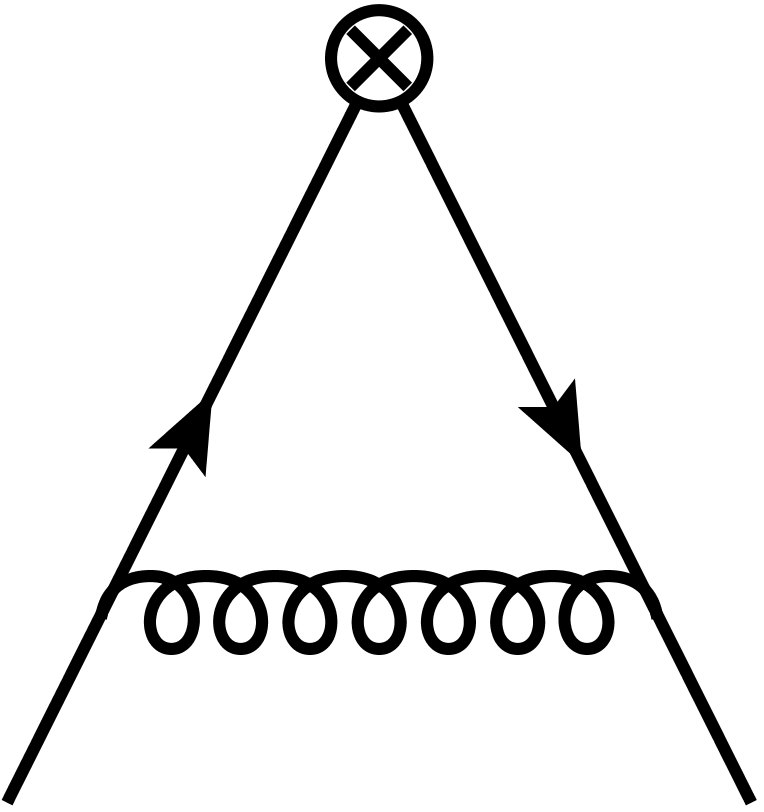
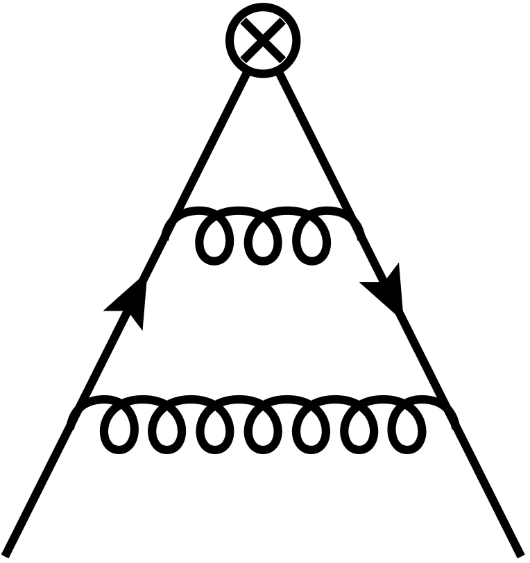
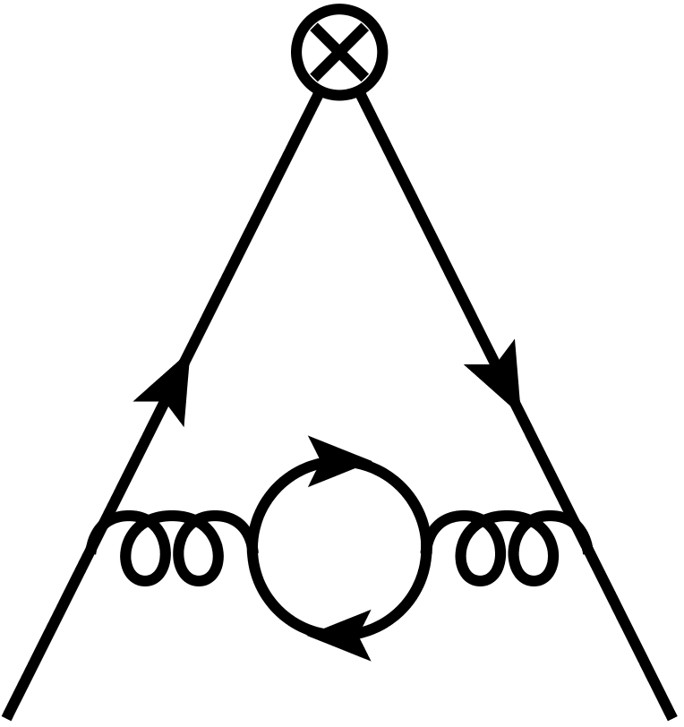
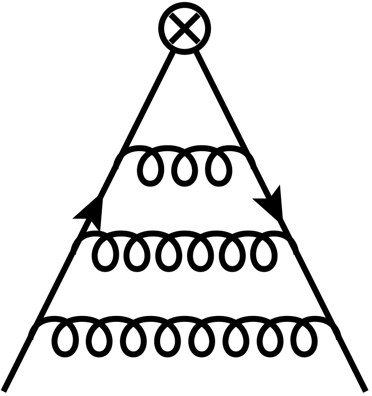
(a)	(b)	(c)	(d)
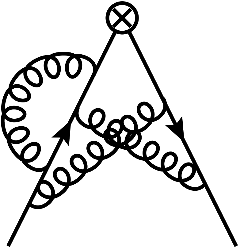
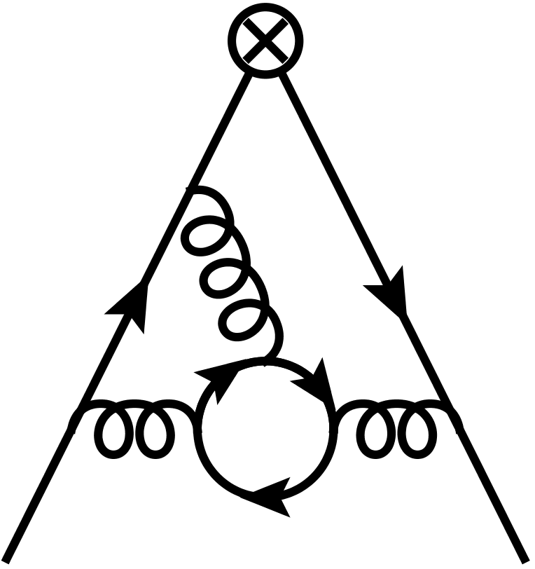
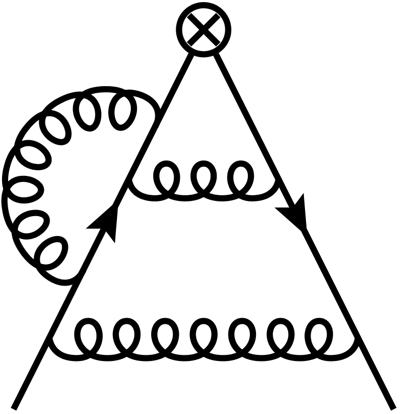
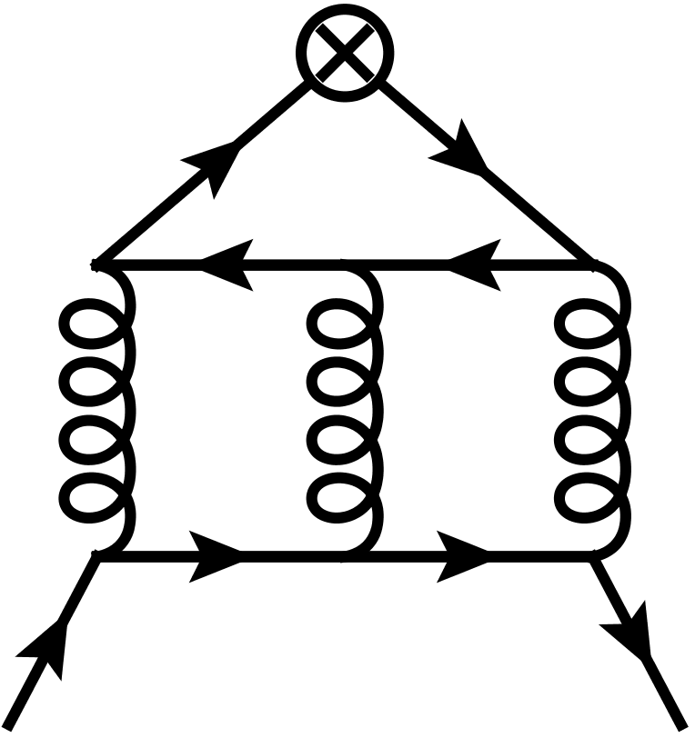
(e)	(f)	(g)	(h)

Figure 1: Sample Feynman diagrams at one-, two- and three-loop order for the current-quark-anti-quark vertex corrections. Solid and curly lines denote quarks and gluons, respectively. The cross represents the coupling to the external current. In this work we only consider non-singlet contributions (a)-(g) and neglect the singlet contributions (h).

Starting point for the matching calculation are the vector, axial-vector, scalar and pseudo-scalar currents in QCD which we define as

$$j_{v}^{\mu} = \bar{\psi}\gamma^{\mu}\psi\,,$$

$$j_{a}^{\mu} = \bar{\psi}\gamma^{\mu}\gamma_{5}\psi\,,$$

$$j_{s} = \bar{\psi}\psi\,,$$

$$j_{p} = \bar{\psi}{\rm i}\gamma_{5}\psi\,.$$ (1)

Note that the anomalous dimensions of the vector and axial-vector current are zero whereas $j_{s}$ and $j_{p}$ involve non-trivial renormalization constants.

Expanding the spinors in Eq. (1) for $|\vec{p}\,|\ll m$, where $\vec{p}$ is the momentum of the anti-quark in the final state, one finds the currents in the effective theory,

$$\tilde{j}_{v}^{k} = \phi^{\dagger}\sigma^{k}\chi\,,$$

$$\tilde{j}_{a}^{k} = \frac{1}{2m}\phi^{\dagger}[\sigma^{k},\vec{p}\cdot\vec{\sigma}]\chi\,,$$

$$\tilde{j}_{s} = -\frac{1}{m}\phi^{\dagger}\vec{p}\cdot\vec{\sigma}\chi\,,$$

$$\tilde{j}_{p} = -{\rm i}\phi^{\dagger}\chi\,,$$ (2)

where $\phi$ and $\chi$ are two-component Pauli spinors.

The currents in Eqs. (1) and (2) are used to form renormalized vertex functions with two external on-shell quarks which we denote by $\Gamma_{x}(q_{1},q_{2})$ and $\tilde{\Gamma}_{x}$ with $x\in\{v,a,s,p\}$, respectively. $q_{1}$ and $q_{2}$ correspond to the momenta of the quark and anti-quark with $q_{1}^{2}=q_{2}^{2}=m^{2}$ where $m$ is the quark mass. We apply an asymptotic expansion around $s=4m^{2}$ Beneke:1997zp ; Smirnov:2002pj , where $s$ is the momentum squared of the external current, which leads to

$$Z_{2}Z_{x}\Gamma_{x}(q_{1},q_{2}) = c_{x}\tilde{Z}_{2}\tilde{Z}_{x}^{-1}\tilde{\Gamma}_{x}+\ldots\,.$$ (3)

The ellipses denote terms suppressed by at least two inverse powers of the heavy quark mass. It is understood that $\Gamma_{x}(q_{1},q_{2})$ is expressed in terms of the heavy quark mass in the on-shell scheme and the strong coupling in the $\overline{\rm MS}$ scheme. $Z_{2}$ and $\tilde{Z}_{2}$ are the on-shell wave function renormalization constants. $Z_{2}$ is needed up to three loops Melnikov:2000zc ; Marquard:2007uj whereas $\tilde{Z}_{2}=1$ since the quantum corrections in NRQCD only involve scaleless integrals which are set to zero in dimensional regularization. Also for $\tilde{\Gamma}_{x}$ only tree-level contributions are needed since the soft, potenial and ultrasoft contributions are present on both sides of Eq. (3) and cancel such that only the hard contribution of $\Gamma_{x}(q_{1},q_{2})$ has to be computed. $Z_{x}$ is the renormalization constant of the current in full QCD which is given by $Z_{v}=Z_{a}=1$ and $Z_{s}=Z_{p}=Z_{m}$. Here $Z_{m}$ is the on-shell quark mass renormalization constant defined via $m=Z_{m}m^{0}$, where $m_{0}$ is the bare heavy quark mass. $\tilde{Z}_{x}$ is the renormalization constant of the current in NRQCD which is determined from the infrared divergences of $c_{x}$. $\tilde{Z}_{x}$ deviates from 1 starting at order $\alpha_{s}^{2}$. The computation of the matching coefficient $c_{x}$ is the main purpose of this work.

Two-loop corrections to $c_{v}$ have been computed for the first time in Refs. Czarnecki:1997vz ; Beneke:1997jm and in Ref. Kniehl:2006qw two-loop corrections to all four currents have been considered, including the singlet contributions. Three-loop corrections to $c_{v}$ have been computed in Refs. Marquard:2006qi ; Marquard:2009bj ; Marquard:2014pea . In these works the reduction to master integrals has been performed analytically. However, most of the master integrals have only been computed numerically with the help of FIESTA Smirnov:2015mct . As a consequence the coefficients of some colour structures are only know with an uncertainty of a few percent. This is sufficient for most phenomenological applications. It is nevertheless desirable to have an independent cross check with improved accuracy. This is provided in this work.

In the next Section we provide details on our calculation and describe our method to extract the matching coefficient from results for the form factors. In Section III we present our results for the matching coefficients and the anomalous dimension of the currents in the effective theory. Section IV contains a brief summary.

II Technical details

For the computation of the hard part of the vertex diagrams we apply the method developed in Ref. Fael:2021kyg . We profit from the findings of Refs. Fael:2022rgm ; FLSS22 where results for massive form factors with external vector, axial-vector, scalar and pseudo-scalar currents have been computed. They can be decomposed into six form factors given by

$$\Gamma_{\mu}^{v}(q_{1},q_{2}) = F_{1}^{v}(s)\gamma_{\mu}-\frac{\mathrm{i}}{2m}F_{2}^{v}(s)\sigma_{\mu\nu}q^{\nu}\,,$$

$$\Gamma_{\mu}^{a}(q_{1},q_{2}) = F_{1}^{a}(s)\gamma_{\mu}\gamma_{5}{-\frac{1}{2m}F_{2}^{a}(s)q_{\mu}}\gamma_{5}\,,$$

$$\Gamma^{s}(q_{1},q_{2}) = {m}F^{s}(s)\,,$$

$$\Gamma^{p}(q_{1},q_{2}) = {\mathrm{i}m}F^{p}(s){\gamma_{5}}\,,$$ (4)

where $\sigma^{\mu\nu}=\mathrm{i}[\gamma^{\mu},\gamma^{\nu}]/2$ and $s$ is the invariant mass of the external current. The quantity $\Gamma_{x}(q_{1},q_{2})$ in Eq. (3) is obtained from the hard part of the form factors evaluated at $s=4m^{2}$ through

$$\Gamma_{v} = (F_{1}^{v}+F_{2}^{v})\big{|}_{\rm hard,\,s=4m^{2}}\,,$$

$$\Gamma_{a} = F_{1}^{a}\big{|}_{\rm hard,\,s=4m^{2}}\,,$$

$$\Gamma_{s} = F^{s}\big{|}_{\rm hard,\,s=4m^{2}}\,,$$

$$\Gamma_{p} = F^{p}\big{|}_{\rm hard,\,s=4m^{2}}\,,$$ (5)

which is discussed in more detail in the remainder of this section.

The basic idea of Ref. Fael:2021kyg is to construct expansions of the master integrals for various values of $s/m^{2}$ with the help of the corresponding differential equations. The unconstrained coefficients of the expansions are fixed by matching two neighboring expressions at an intermediate point. The starting point in Refs. Fael:2022rgm ; FLSS22 is $s=0$ where all master integrals can be computed analytically. In order to arrive at the threshold $s=4m^{2}$ we perform expansions for $s/m^{2}=1,2,5/2,3,7/2$ and $4$.

The expansion around $s/m^{2}=4$ uses the variable

$$x =\sqrt{4-\frac{s}{m^{2}}}\,.$$ (6)

It contains both even and odd powers of $x$ accompanied by $\ln(x)$ terms, since it comprises the contributions from all regions present close to threshold. In particular, each loop momentum can have one of the following scalings Beneke:1997zp :

• hard (h): $k_{0}\sim m$, $k_{i}\sim m$ ,

• potential (p): $k_{0}\sim x^{2}\cdot m$, $k_{i}\sim x\cdot m$ ,

• soft (s): $k_{0}\sim x\cdot m$, $k_{i}\sim x\cdot m$ ,

• ultrasoft (u): $k_{0}\sim x^{2}\cdot m$, $k_{i}\sim x^{2}\cdot m$ .

For the matching coefficients we only need the region where all loop momenta are hard. Here only even powers of $x$ and no $\ln(x)$ terms are present.

Using the scalings from above, we see that in each region the integral is given as $x^{-n\,\epsilon}$ multiplied by a Taylor expansion in $x$, with an integer $n$ which can be derived from the scaling of the loop momenta in the respective region. Here $\epsilon=(4-d)/2$ where $d$ is the space-time dimension. We can insert this ansatz into the system of differential equations for the master integrals and obtain a system of linear equations for the expansion coefficients. For each region the system is reduced to a small set of undetermined boundary constants with the help of a version of Kira Maierhofer:2017gsa ; Klappert:2020nbg with FireFly Klappert:2019emp ; Klappert:2020aqs optimized for solving systems without variables. After summing the contributions from all regions we obtain again the results for the master integrals in full kinematics. We can therefore numerically match the yet undetermined boundary constants with the numerical results computed in Ref. Fael:2022rgm . Substituting the numerical solutions into the ansatz for the $x^{-0\,\epsilon}$ scaling provides the master integrals in the hard expansion.

Let us in the following discuss the calculation in more detail. At two-loop order we find the following scalings for the different regions:

• $x^{-0\epsilon}$: (h-h),

• $x^{-2\epsilon}$: (h-p), (h-s),

• $x^{-4\epsilon}$: (h-u), (p-p), (s-s), (p-s),

• $x^{-6\epsilon}$: (p-u), (s-u),

• $x^{-8\epsilon}$: (u-u),

where the list on the right of the colon specifies the scaling of the two loop momenta. Some of the combinations might vanish due to the presence of scaleless integrals. However, in our approach we do not have to pay attention to this. Since only the spacial parts get continued into $(d-1)$ dimensions, potential and soft regions of the loop momenta lead to the same $\epsilon$-dimensional scalings. The pure ultrasoft region $\sim x^{-8\epsilon}$ does not contribute which we checked by an explicit calculation. For the two-loop calculation we therefore have to consider four independent expansions. Note that the individual regions contributing to one of the $x^{-n\epsilon}$ scalings might develop higher poles in the dimensional regulator $\epsilon$ than the sum. These higher poles lead to Sudakov-like double logarithms which are not present in the threshold expansion considered here. We therefore do not have to extend the ansatz to higher poles in $\epsilon$ compared to the full calculation in Ref. Fael:2022rgm .

At three loop order we have the scalings

• $x^{-0\epsilon}$: (h-h-h),

• $x^{-2\epsilon}$: (h-h-p), (h-h-s),

• $x^{-4\epsilon}$: (h-h-u), (h-p-p), (h-s-s), (h-p-s),

• $x^{-6\epsilon}$: (h-p-u), (h-s-u), (p-p-p), (p-p-s), (p-s-s), (s-s-s),

• $x^{-8\epsilon}$: (h-u-u), (u-p-p), (u-p-s), (u-s-s),

• $x^{-10\epsilon}$: (u-u-p), (u-u-s),

• $x^{-12\epsilon}$: (u-u-u),

which means that we have to construct six independent expansions since the pure-ultrasoft contribution vanishes. After the reduction to boundary constants we are left with $(568,125,248,402,236,51)$ undetermined coefficients for the scalings $x^{-0\epsilon},\ldots,x^{-10\epsilon}$. They can be reduced by utilizing information about the master integrals from the full calculation. On the one hand, we know some integrals analytically, especially those which do not depend on $s$. They can be fixed from the expansion around $s=0$. Furthermore, some of the $\epsilon$ poles also do not have a $s$ dependence and thus also they are available from the calculation performed for $s=0$. On the other hand, we know the leading power in $x$ for each integral from the full result. This knowledge implies relations between the boundary constants from different regions which leads to a reduction of the number of independent boundary constants from 1630 to 578. They are determined as follows: After obtaining the symbolic expansions for each region we equate the sum of all regions with the numerical evaluation of the full result at $s=3.75m^{2}$ from Ref. Fael:2022rgm and solve the resulting linear system for the 578 boundary constants. In particular all 568 coefficients from the pure-hard regions of all 422 master integrals are obtained by this procedure, whereas the regions which scale as $x^{-n\epsilon}$ with $n>0$ can not be disentangled. This is sufficient for the application in the present paper.

Let us mention that in case one wants to construct results for each individual region further information is needed. It can be obtained by determining for each region of every master integral the leading power in $x$. Here the program asy.m Pak:2010pt ; Jantzen:2012mw can be used. In this way one obtains relations for each individual region instead of only for the sum of all of them.

Next we insert the hard regions of the master integrals into the amplitudes for the form factors. It contains terms scaling with inverse powers of $(s-4m^{2})$ from the reduction of the master integrals with full kinematics. It is a non-trivial check that the limit $s\to 4m^{2}$ exists. In fact we have checked that all inverse powers of $(s-4m^{2})$ have coefficients below $3\cdot 10^{-11}$ which is the precision of our calculation. Inserting the form factors into Eq. (5) we finally obtain the vertex functions $\Gamma_{x}$ entering the matching equation (3). As a further check we keep the QCD gauge parameter $\xi$ and observe that it vanishes after renormalization.

III Three-loop matching coefficients

Once all ingredients for the left-hand-side of Eq. (3) are available we can solve it for $c_{x}$ order-by-order in $\alpha_{s}$. At one-loop order all quantities with a tilde on the right-hand-side are equal to 1. At order $\alpha_{s}^{2}$ infrared divergences are left on the left-hand-side which are absorbed into $\tilde{Z}_{x}$. Finally, at order $\alpha_{s}^{3}$ one has to take care of the interference term of $\tilde{Z}_{x}^{-1}$ and the one-loop result of $c_{x}$, which is needed up to order $\epsilon$. The remaining infrared divergences are again absorbed into $\tilde{Z}_{x}$. We parametrize the perturbative results in this section by the strong coupling in the effective theory with $n_{l}$ active quark flavours which we denote by $\alpha_{s}^{(n_{l})}$.

Let us in a first step provide the results for the renormalization constants which are obtained by subtracting the remaining infrared divergences in a minimal way. For the vector current we have

$$\tilde{Z}_{v} = 1+\left(\frac{\alpha_{s}^{(n_{l})}(\mu)}{\pi}\right)^{2}\frac{C_{F}\pi^{2}}{\epsilon}\left(\frac{1}{12}C_{F}+\frac{1}{8}C_{A}\right)+\left(\frac{\alpha_{s}^{(n_{l})}(\mu)}{\pi}\right)^{3}C_{F}\pi^{2}\Bigg{\{}C_{F}^{2}\left[\frac{5}{144\epsilon^{2}}+\left(\frac{43}{144}-\frac{1}{2}l_{2}+\frac{5}{48}L_{\mu}\right)\frac{1}{\epsilon}\right]$$ (7)

$$\mbox{}+C_{F}C_{A}\left[\frac{1}{864\epsilon^{2}}+\left(\frac{113}{324}+\frac{1}{4}l_{2}+\frac{5}{32}L_{\mu}\right)\frac{1}{\epsilon}\right]+C_{A}^{2}\left[-\frac{1}{16\epsilon^{2}}+\left(\frac{2}{27}+\frac{1}{4}l_{2}+\frac{1}{24}L_{\mu}\right)\frac{1}{\epsilon}\right]$$

$$\mbox{}+Tn_{l}\left[C_{F}\left(\frac{1}{54\epsilon^{2}}-\frac{25}{324\epsilon}\right)+C_{A}\left(\frac{1}{36\epsilon^{2}}-\frac{37}{432\epsilon}\right)\right]+C_{F}Tn_{h}\frac{1}{60\epsilon}\Bigg{\}}+{\cal O}(\alpha_{s}^{4})\,,$$

which agrees with the explicit calculations in the effective theory from Refs. Beneke:1997jm ; Marquard:2006qi ; Kniehl:2002yv ; Beneke:2007pj . In Eq. (7) $C_{F}=(N_{c}^{2}-1)/(2N_{c})$ and $C_{A}=2TN_{c}$ are the quadratic Casimir operators of the $\mathrm{SU}(N_{c})$ gauge group in the fundamental and adjoint representation, respectively, $n_{l}$ is the number of massless quark flavors, and $T=1/2$. Furthermore we have $L_{\mu}=\ln(\mu^{2}/m^{2})$ and $l_{2}=\ln(2)$.

For the remaining three currents our results read

$$\tilde{Z}_{a} = 1+\left(\frac{\alpha_{s}^{(n_{l})}(\mu)}{\pi}\right)^{2}\frac{C_{F}\pi^{2}}{\epsilon}\left(\frac{1}{24}C_{A}+\frac{5}{48}C_{F}\right)+\left(\frac{\alpha_{s}^{(n_{l})}(\mu)}{\pi}\right)^{3}C_{F}\pi^{2}\Biggr{\{}C_{F}^{2}\left(\frac{215}{864}-\frac{l_{2}}{3}\right)\frac{1}{\epsilon}$$

$$+C_{F}C_{A}\left[-\frac{25}{576\epsilon^{2}}+\left(\frac{1}{18}l_{2}+\frac{35}{576}L_{\mu}+\frac{1433}{5184}\right)\frac{1}{\epsilon}\right]+C_{A}^{2}\left[-\frac{1}{48\epsilon^{2}}+\left(\frac{5}{36}l_{2}+\frac{1}{72}L_{\mu}+\frac{17}{324}\right)\frac{1}{\epsilon}\right]$$

$$+Tn_{l}\left[C_{F}\left(\frac{5}{216\epsilon^{2}}-\frac{83}{1296\epsilon}\right)+C_{A}\left(\frac{1}{108\epsilon^{2}}-\frac{53}{1296\epsilon}\right)\right]\Biggr{\}}\,,$$

$$\tilde{Z}_{s} = 1+\left(\frac{\alpha_{s}^{(n_{l})}(\mu)}{\pi}\right)^{2}\frac{C_{F}\pi^{2}}{\epsilon}\left(\frac{1}{24}C_{A}+\frac{1}{6}C_{F}\right)+\left(\frac{\alpha_{s}^{(n_{l})}(\mu)}{\pi}\right)^{3}C_{F}\pi^{2}\Biggr{\{}C_{F}^{2}\left(\frac{65}{216}-\frac{1}{3}l_{2}\right)\frac{1}{\epsilon}$$

$$+C_{F}C_{A}\left[-\frac{7}{96\epsilon^{2}}+\left(\frac{461}{1296}+\frac{1}{18}l_{2}+\frac{25}{288}L_{\mu}\right)\frac{1}{\epsilon}\right]+C_{A}^{2}\left[-\frac{1}{48\epsilon^{2}}+\left(\frac{17}{324}+\frac{5}{36}l_{2}+\frac{1}{72}L_{\mu}\right)\frac{1}{\epsilon}\right]$$

$$+Tn_{l}\left[C_{F}\left(\frac{1}{27\epsilon^{2}}-\frac{29}{324\epsilon}\right)+C_{A}\left(\frac{1}{108\epsilon^{2}}-\frac{53}{1296\epsilon}\right)\right]\Biggr{\}}\,,$$

$$\tilde{Z}_{p} = 1+\left(\frac{\alpha_{s}^{(n_{l})}(\mu)}{\pi}\right)^{2}\frac{C_{F}\pi^{2}}{\epsilon}\left(\frac{1}{8}C_{A}+\frac{1}{4}C_{F}\right)+\left(\frac{\alpha_{s}^{(n_{l})}(\mu)}{\pi}\right)^{3}C_{F}\pi^{2}\Biggr{\{}C_{F}^{2}\left[\frac{5}{144\epsilon^{2}}+\left(\frac{31}{144}-\frac{1}{2}l_{2}+\frac{5}{48}L_{\mu}\right)\frac{1}{\epsilon}\right]$$ (8)

$$+C_{F}C_{A}\left[-\frac{5}{96\epsilon^{2}}+\left(\frac{199}{432}+\frac{1}{4}l_{2}+\frac{29}{96}L_{\mu}\right)\frac{1}{\epsilon}\right]+C_{A}^{2}\left[-\frac{1}{16\epsilon^{2}}+\left(\frac{2}{27}+\frac{1}{4}l_{2}+\frac{1}{24}L_{\mu}\right)\frac{1}{\epsilon}\right]$$

$$+Tn_{l}\left[C_{F}\left(\frac{1}{18\epsilon^{2}}-\frac{11}{108\epsilon}\right)+C_{A}\left(\frac{1}{36\epsilon^{2}}-\frac{37}{432\epsilon}\right)\right]+C_{F}Tn_{h}\frac{1}{60\epsilon}\Biggr{\}}\,.$$

Note that our method only provides numerical results for the pole parts. However, the precision is sufficiently high such that the analytic results can be reconstructed using the PSLQ algorithm PSLQ .

The renormalization constants are related to the anomalous dimensions via

$$\gamma_{x}=\frac{\mathrm{d}\ln(\tilde{Z}_{x})}{\mathrm{d}\ln(\mu)}~{},$$ (9)

which leads to

$$\gamma_{x}=-4\left(\frac{\alpha_{s}^{(n_{l})}}{\pi}\right)^{2}\tilde{Z}_{x}^{(2,-1)}-6\left(\frac{\alpha_{s}^{(n_{l})}}{\pi}\right)^{3}\tilde{Z}_{x}^{(3,-1)}+{\cal O}(\alpha_{s}^{4})~{},$$ (10)

where $\tilde{Z}_{x}^{(a,b)}$ denotes the contribution to $\tilde{Z}$ at order $\alpha_{s}^{a}\epsilon^{b}$.

For the perturbative expansion of $c_{x}$ we set the renormalization scale of the strong coupling constant to $\mu^{2}=m^{2}$ and write

$$c_{x} = 1+\frac{\alpha_{s}^{(n_{l})}(m)}{\pi}c_{x}^{(1)}+\left(\frac{\alpha_{s}^{(n_{l})}(m)}{\pi}\right)^{2}c_{x}^{(2)}+\left(\frac{\alpha_{s}^{(n_{l})}(m)}{\pi}\right)^{3}c_{x}^{(3)}+{\cal O}(\alpha_{s}^{4})\,.$$ (11)

The three-loop coefficient is further decomposed according to the color structures as

$$c_{x}^{(3)} = C_{F}\big{[}C_{F}^{2}c^{x}_{FFF}+C_{F}C_{A}c^{x}_{FFA}+C_{A}^{2}c^{x}_{FAA}+Tn_{l}\left(C_{F}c^{x}_{FFL}+C_{A}c^{x}_{FAL}+Tn_{h}c^{x}_{FHL}+Tn_{l}c^{x}_{FLL}\right)$$ (12)

$$\mbox{}+Tn_{h}\left(C_{F}c^{x}_{FFH}+C_{A}c^{x}_{FAH}+Tn_{h}c^{x}_{FHH}\right)\big{]}+\mbox{singlet terms}\,.$$

In the following we present result for $c_{x}$ where for completeness also the one- and two-loop results are shown. For the vector current our results read:

$$c_{v}^{(1)} = -2C_{F}\,,$$

$$c_{v}^{(2)} = \left(-\frac{151}{72}+\frac{89}{144}\pi^{2}-\frac{5}{6}\pi^{2}l_{2}-\frac{13}{4}\zeta(3)\right)C_{A}C_{F}+\left(\frac{23}{8}-\frac{79}{36}\pi^{2}+\pi^{2}l_{2}-\frac{1}{2}\zeta(3)\right)C_{F}^{2}$$

$$\mbox{}+\left(\frac{22}{9}-\frac{2}{9}\pi^{2}\right)C_{F}Tn_{h}+\frac{11}{18}C_{F}Tn_{l}-\frac{1}{2}\pi^{2}\left(\frac{1}{2}C_{A}+\frac{1}{3}C_{F}\right)C_{F}L_{\mu}\,,$$

$$c^{v}_{FFF} = 36.49486246+\left(-\frac{9}{16}+\frac{3}{2}l_{2}\right)\pi^{2}L_{\mu}-\frac{5}{32}\pi^{2}L_{\mu}^{2}\,,$$

$$c^{v}_{FFA} = -188.0778417+\left(-\frac{59}{108}-\frac{3}{4}l_{2}\right)\pi^{2}L_{\mu}-\frac{47}{576}\pi^{2}L_{\mu}^{2}\,,$$

$$c^{v}_{FAA} = -97.73497327+\left(-\frac{2}{9}-\frac{3}{4}l_{2}\right)\pi^{2}L_{\mu}+\frac{1}{6}\pi^{2}L_{\mu}^{2}\,,$$

$$c^{v}_{FFL} = 46.69169291+\frac{25}{108}\pi^{2}L_{\mu}-\frac{1}{18}\pi^{2}L_{\mu}^{2}\,,$$

$$c^{v}_{FAL} = 39.62371855+\frac{37}{144}\pi^{2}L_{\mu}-\frac{1}{12}\pi^{2}L_{\mu}^{2}\,,$$

$$c^{v}_{FHL} = -\frac{557}{162}+\frac{26}{81}\pi^{2}\,,$$

$$c^{v}_{FLL} = -\frac{163}{162}-\frac{4}{27}\pi^{2}\,,$$

$$c^{v}_{FFH} = -0.8435622912-\frac{1}{20}\pi^{2}L_{\mu}\,,$$

$$c^{v}_{FAH} = -0.1024741615\,,$$

$$c^{v}_{FHH} = -\frac{427}{162}+\frac{158}{2835}\pi^{2}+\frac{16}{9}\zeta(3)\,,$$ (13)

The coefficient of the logaritmic contributions and the coefficients $c^{v}_{FHL}$ and $c^{v}_{FLL}$ have been reconstructed using our numerical expressions. They agree with the results presented in Ref. Marquard:2014pea . Our numerical precision is not sufficient to obtain the analytic expressions for $c^{v}_{FHH}$ which we take from Ref. Marquard:2014pea . For all coefficients presented in numerical form we have a precision of at least ten digits, which is a significant improvement. For example, for the non-fermionic coefficients the results in Ref. Marquard:2014pea read $c^{v}_{FFF}=36.55(0.53)$, $c^{v}_{FFA}=-188.10(0.83)$ and $c^{v}_{FAA}=-97.81(0.38)$.

For the remaining three currents we have

$$c_{a}^{(1)} = -C_{F}\,,$$

$$c_{a}^{(2)} = \left(-\frac{9}{8}\zeta(3)+\frac{35}{144}\pi^{2}-\frac{101}{72}-\frac{7}{12}\pi^{2}l_{2}\right)C_{A}C_{F}+\left(-\frac{27}{16}\zeta(3)-\frac{9}{8}\pi^{2}+\frac{23}{24}+\frac{19}{24}\pi^{2}l_{2}\right)C_{F}^{2}$$

$$\mbox{}+\left(\frac{20}{9}-\frac{2}{9}\pi^{2}\right)C_{F}Tn_{h}+\frac{7}{18}C_{F}Tn_{l}+\pi^{2}\left(-\frac{1}{12}C_{A}-\frac{5}{24}C_{F}\right)C_{F}L_{\mu}\,,$$

$$c^{a}_{FFF} = -4.764274486+\left(-\frac{155}{288}+l_{2}\right)\pi^{2}L_{\mu}\,,$$

$$c^{a}_{FFA} = -83.88648515+\left(-\frac{1289}{1728}-\frac{1}{6}l_{2}\right)\pi^{2}L_{\mu}+\frac{115}{1152}\pi^{2}L_{\mu}^{2}\,,$$

$$c^{a}_{FAA} = -63.00619439+\left(-\frac{17}{108}-\frac{5}{12}l_{2}\right)\pi^{2}L_{\mu}+\frac{1}{18}\pi^{2}L_{\mu}^{2}\,,$$

$$c^{a}_{FFL} = 28.13543651+\frac{83}{432}\pi^{2}L_{\mu}-\frac{5}{72}\pi^{2}L_{\mu}^{2}\,,$$

$$c^{a}_{FAL} = 23.17119085+\frac{53}{432}\pi^{2}L_{\mu}-\frac{1}{36}\pi^{2}L_{\mu}^{2}\,,$$

$$c^{a}_{FHL} = -\frac{415}{162}+\frac{20}{81}\pi^{2}\,,$$

$$c^{a}_{FLL} = -\frac{65}{162}-\frac{2}{27}\pi^{2}\,,$$

$$c^{a}_{FFH} = 0.8971357511\,,$$

$$c^{a}_{FAH} = -0.2169123942\,,$$

$$c^{a}_{FHH} = -0.01136428050\,,$$ (14)

$$c_{s}^{(1)} = -\frac{1}{2}C_{F}\,,$$

$$c_{s}^{(2)} = \left(-\frac{5}{4}\zeta(3)+\frac{1}{48}\pi^{2}+\frac{49}{144}-\frac{1}{2}\pi^{2}l_{2}\right)C_{A}C_{F}+\left(-\frac{11}{4}\zeta(3)-\frac{37}{48}\pi^{2}+\frac{5}{16}+\frac{1}{2}\pi^{2}l_{2}\right)C_{F}^{2}$$

$$\mbox{}+\left(\frac{121}{36}-\frac{1}{3}\pi^{2}\right)C_{F}Tn_{h}-\frac{5}{36}C_{F}Tn_{l}+\pi^{2}\left(-\frac{1}{12}C_{A}-\frac{1}{3}C_{F}\right)C_{F}L_{\mu}\,,$$

$$c^{s}_{FFF} = -11.17444530+\left(-\frac{53}{72}+l_{2}\right)\pi^{2}L_{\mu}\,,$$

$$c^{s}_{FFA} = -83.13918787+\left(-\frac{443}{432}-\frac{1}{6}l_{2}\right)\pi^{2}L_{\mu}+\frac{101}{576}\pi^{2}L_{\mu}^{2}\,,$$

$$c^{s}_{FAA} = -67.24288900+\left(-\frac{17}{108}-\frac{5}{12}l_{2}\right)\pi^{2}L_{\mu}+\frac{1}{18}\pi^{2}L_{\mu}^{2}\,,$$

$$c^{s}_{FFL} = 30.10118322+\frac{29}{108}\pi^{2}L_{\mu}-\frac{1}{9}\pi^{2}L_{\mu}^{2}\,,$$

$$c^{s}_{FAL} = 21.41321398+\frac{53}{432}\pi^{2}L_{\mu}-\frac{1}{36}\pi^{2}L_{\mu}^{2}\,,$$

$$c^{s}_{FHL} = -\frac{157}{81}+\frac{5}{27}\pi^{2}\,,$$

$$c^{s}_{FLL} = \frac{73}{324}-\frac{1}{27}\pi^{2}\,,$$

$$c^{s}_{FFH} = 1.879249909\,,$$

$$c^{s}_{FAH} = -0.3740808359\,,$$

$$c^{s}_{FHH} = 0.007237324266\,,$$ (15)

$$c_{p}^{(1)} = -\frac{3}{2}C_{F}\,,$$

$$c_{p}^{(2)} = \left(-3\zeta(3)+\frac{17}{48}\pi^{2}-\frac{17}{48}-\pi^{2}l_{2}\right)C_{A}C_{F}+\left(-\frac{9}{2}\zeta(3)-\frac{79}{48}\pi^{2}+\frac{29}{16}+\pi^{2}l_{2}\right)C_{F}^{2}$$

$$\mbox{}+\left(\frac{43}{12}-\frac{1}{3}\pi^{2}\right)C_{F}Tn_{h}+\frac{1}{12}C_{F}Tn_{l}+\pi^{2}\left(-\frac{1}{4}C_{A}-\frac{1}{2}C_{F}\right)C_{F}L_{\mu}\,,$$

$$c^{p}_{FFF} = -16.65729478+\left(\frac{5}{48}+\frac{3}{2}l_{2}\right)\pi^{2}L_{\mu}-\frac{5}{32}\pi^{2}L_{\mu}^{2}\,,$$

$$c^{p}_{FFA} = -181.0487647+\left(-\frac{145}{144}-\frac{3}{4}l_{2}\right)\pi^{2}+\frac{1}{192}\pi^{2}L_{\mu}^{2}\,,$$

$$c^{p}_{FAA} = -104.3591595+\left(-\frac{2}{9}-\frac{3}{4}l_{2}\right)\pi^{2}L_{\mu}+\frac{1}{6}\pi^{2}L_{\mu}^{2}\,,$$

$$c^{p}_{FFL} = 51.93841187+\frac{11}{36}\pi^{2}L_{\mu}-\frac{1}{6}\pi^{2}L_{\mu}^{2}\,,$$

$$c^{p}_{FAL} = 39.92104383+\frac{37}{144}\pi^{2}L_{\mu}-\frac{1}{12}\pi^{2}L_{\mu}^{2}\,,$$

$$c^{p}_{FHL} = -\frac{76}{27}+\frac{7}{27}\pi^{2}\,,$$

$$c^{p}_{FLL} = -\frac{41}{108}-\frac{1}{9}\pi^{2}\,,$$

$$c^{p}_{FFH} = 3.081762039-\frac{1}{20}\pi^{2}L_{\mu}\,,$$

$$c^{p}_{FAH} = -0.8953812450\,,$$

$$c^{p}_{FHH} = 0.06984121227\,.$$ (16)

For the axial-vector, scalar and pseudo-scalar current the terms proportional to $n_{l}$ and $n_{l}^{2}$ can be found in Ref. Piclum:2007an . There, the non-logarithmic terms of the coefficients $c^{x}_{FFL}$ and $c^{x}_{FAL}$ only have a precision of two significant digits whereas we have a precision of at least ten digits. Our analytic results for $c^{x}_{FHL}$ and $c^{x}_{FLL}$ agree with Piclum:2007an .

After specifying the number of colours to three we have for $\mu^{2}=m^{2}$ and $n_{h}=1$

$$c_{v} \approx 1-\frac{\alpha_{s}^{(n_{l})}}{\pi}\cdot 2.66667+\left(\frac{\alpha_{s}^{(n_{l})}}{\pi}\right)^{2}\left[-44.5510+0.407407\,n_{l}\right]+\left(\frac{\alpha_{s}^{(n_{l})}}{\pi}\right)^{3}\left[-2090.33+120.661\,n_{l}-0.822779\,n_{l}^{2}\right]$$

$$\mbox{}+\mbox{singlet terms}\,,$$

$$c_{a} \approx 1-\frac{\alpha_{s}^{(n_{l})}}{\pi}\cdot 1.33333+\left(\frac{\alpha_{s}^{(n_{l})}}{\pi}\right)^{2}\left[-29.3816+0.259259\,n_{l}\right]+\left(\frac{\alpha_{s}^{(n_{l})}}{\pi}\right)^{3}\left[-1214.40+71.3101\,n_{l}-0.377439\,n_{l}^{2}\right]$$

$$\mbox{}+\mbox{singlet terms}\,,$$

$$c_{s} \approx 1-\frac{\alpha_{s}^{(n_{l})}}{\pi}\cdot 0.666667+\left(\frac{\alpha_{s}^{(n_{l})}}{\pi}\right)^{2}\left[-30.2266-0.0925926\,n_{l}\right]+\left(\frac{\alpha_{s}^{(n_{l})}}{\pi}\right)^{3}\left[-1275.89+69.5462\,n_{l}-0.0467441\,n_{l}^{2}\right]$$

$$\mbox{}+\mbox{singlet terms}\,,$$

$$c_{p} \approx 1-\frac{\alpha_{s}^{(n_{l})}}{\pi}\cdot 2+\left(\frac{\alpha_{s}^{(n_{l})}}{\pi}\right)^{2}\left[-52.1381+0.0555556\,n_{l}\right]+\left(\frac{\alpha_{s}^{(n_{l})}}{\pi}\right)^{3}\left[-2256.42+125.924\,n_{l}-0.492084\,n_{l}^{2}\right]$$ (17)

$$\mbox{}+\mbox{singlet terms}\,.$$

For all four currents the quantum corrections are quite sizable. For applications in the top quark sector, i.e. for $n_{l}=5$, the two- and three-loop corrections have the same order of magnitude as the one-loop term. For $n_{l}=3$ and $n_{l}=4$ the higher order corrections are even larger. Since the matching coefficients on their own are no physical quantities this is no principle problem. However, it shows the importance of the three-loop corrections to $c_{x}$, in particular for $c_{v}$ which has important applications in the bottom Beneke:2014qea ; Egner:2021lxd and top sector Beneke:2015kwa .

IV Conclusions

In this work we have computed the three-loop corrections to the QCD-NRQCD matching coefficients for external vector, axial-vector, scalar and pseudo-scalar currents. We consider the corresponding quark form factors and compute the pure-hard part of each master integral using the method of Ref. Fael:2021kyg supplemented with the information from expansions by regions Beneke:1997zp . We obtain precise numerical results for the three-loop coefficients. For the vector current we provide the first independent cross check for $c_{v}$ which has a significant numerical impact to the N³LO predictions for top-quark-pair production in electron-positron annihilation close to threshold and the leptonic decay width of the $\Upsilon(1S)$ meson. Our new result is several orders of magnitude more precise. The three-loop results for $c_{a}$, $c_{s}$ and $c_{p}$ are new.

Acknowledgements. This research was supported by the Deutsche Forschungsgemeinschaft (DFG, German Research Foundation) under grant 396021762 — TRR 257 “Particle Physics Phenomenology after the Higgs Discovery”. The Feynman diagrams were drawn with the help of Axodraw Vermaseren:1994je and JaxoDraw Binosi:2003yf .

References

(1)
P. Marquard, J. H. Piclum, D. Seidel and M. Steinhauser,
Phys. Rev. D 89 (2014), 034027
[arXiv:1401.3004 [hep-ph]].
(3)
M. Beneke, Y. Kiyo and K. Schuller,
[arXiv:1312.4791 [hep-ph]].
(4)
M. Beneke, Y. Kiyo, P. Marquard, A. Penin, J. Piclum and M. Steinhauser,
Phys. Rev. Lett. 115 (2015), 192001
[arXiv:1506.06864 [hep-ph]].
(5)
M. Beneke, Y. Kiyo, P. Marquard, A. Penin, J. Piclum, D. Seidel and M. Steinhauser,
Phys. Rev. Lett. 112 (2014), 151801
[arXiv:1401.3005 [hep-ph]].
(6)
M. Egner, M. Fael, J. Piclum, K. Schönwald and M. Steinhauser,
Phys. Rev. D 104 (2021), 054033
[arXiv:2105.09332 [hep-ph]].
(7)
M. Baker, P. Marquard, A. A. Penin, J. Piclum and M. Steinhauser,
Phys. Rev. Lett. 112 (2014), 120407
[arXiv:1402.0876 [hep-ph]].
(8)
M. Beneke and V. A. Smirnov,
Nucl. Phys. B 522 (1998), 321-344
[arXiv:hep-ph/9711391].
(9)
V. A. Smirnov,
Springer Tracts Mod. Phys. 177 (2002), 1-262.
(10)
K. Melnikov and T. van Ritbergen,
Nucl. Phys. B 591 (2000), 515-546
[arXiv:hep-ph/0005131].
(11)
P. Marquard, L. Mihaila, J. H. Piclum and M. Steinhauser,
Nucl. Phys. B 773 (2007), 1-18
[arXiv:hep-ph/0702185].
(12)
A. Czarnecki and K. Melnikov,
Phys. Rev. Lett. 80 (1998), 2531
[arXiv:hep-ph/9712222].
(13)
M. Beneke, A. Signer and V. A. Smirnov,
Phys. Rev. Lett. 80 (1998), 2535
[arXiv:hep-ph/9712302].
(14)
B. A. Kniehl, A. Onishchenko, J. H. Piclum and M. Steinhauser,
Phys. Lett. B 638 (2006), 209-213
[arXiv:hep-ph/0604072].
(15)
P. Marquard, J. H. Piclum, D. Seidel and M. Steinhauser,
Nucl. Phys. B 758 (2006), 144-160
[arXiv:hep-ph/0607168].
(16)
P. Marquard, J. H. Piclum, D. Seidel and M. Steinhauser,
Phys. Lett. B 678 (2009), 269-275
[arXiv:0904.0920 [hep-ph]].
(17)
A. V. Smirnov,
Comput. Phys. Commun. 204 (2016), 189-199
[arXiv:1511.03614 [hep-ph]].
(18)
M. Fael, F. Lange, K. Schönwald and M. Steinhauser,
JHEP 09 (2021), 152
[arXiv:2106.05296 [hep-ph]].
(19)
M. Fael, F. Lange, K. Schönwald and M. Steinhauser,
[arXiv:2202.05276 [hep-ph]].
(20)
M. Fael, F. Lange, K. Schönwald and M. Steinhauser,
in preparation.
(21)
P. Maierhöfer, J. Usovitsch and P. Uwer,
Comput. Phys. Commun. 230 (2018), 99-112
[arXiv:1705.05610 [hep-ph]].
(22)
J. Klappert, F. Lange, P. Maierhöfer and J. Usovitsch,
Comput. Phys. Commun. 266 (2021), 108024
[arXiv:2008.06494 [hep-ph]].
(23)
J. Klappert and F. Lange,
Comput. Phys. Commun. 247 (2020), 106951
[arXiv:1904.00009 [cs.SC]].
(24)
J. Klappert, S. Y. Klein and F. Lange,
Comput. Phys. Commun. 264 (2021), 107968
[arXiv:2004.01463 [cs.MS]].
(25)
A. Pak and A. Smirnov,
Eur. Phys. J. C 71 (2011), 1626
[arXiv:1011.4863 [hep-ph]].
(26)
B. Jantzen, A. V. Smirnov and V. A. Smirnov,
Eur. Phys. J. C 72 (2012), 2139
[arXiv:1206.0546 [hep-ph]].
(27)
B. A. Kniehl, A. A. Penin, V. A. Smirnov and M. Steinhauser,
Phys. Rev. Lett. 90 (2003), 212001
[erratum: Phys. Rev. Lett. 91 (2003), 139903]
[arXiv:hep-ph/0210161].
(28)
M. Beneke, Y. Kiyo and A. A. Penin,
Phys. Lett. B 653 (2007), 53-59
[arXiv:0706.2733 [hep-ph]].
(29)
H. R. P. Ferguson, D. H. Bailey and S. Arno,
Math. Comp. 68 (1999), 351-369.
(30)
J. H. Piclum,
“Heavy quark threshold dynamics in higher order,”
Dissertation, Hamburg University 2007.
(31)
J. A. M. Vermaseren,
Comput. Phys. Commun. 83 (1994), 45-58.
(32)
D. Binosi and L. Theußl,
Comput. Phys. Commun. 161 (2004), 76-86
[arXiv:hep-ph/0309015].