Magnetic fields in star formation: from clouds to cores

Abstract

In this chapter we review recent advances in understanding the roles that magnetic fields play throughout the star formation process, gained through observations and simulations of molecular clouds, the dense, star-forming phase of the magnetised, turbulent interstellar medium (ISM). Recent results broadly support a picture in which the magnetic fields of molecular clouds transition from being gravitationally sub-critical and near equipartition with turbulence in low-density cloud envelopes, to being energetically sub-dominant in dense, gravitationally unstable star-forming cores. Magnetic fields appear to play an important role in the formation of cloud substructure by setting preferred directions for large-scale gas flows in molecular clouds, and can direct the accretion of material onto star-forming filaments and hubs. Low-mass star formation may proceed in environments close to magnetic criticality; high-mass star formation remains less well-understood, but may proceed in more supercritical environments. The interaction between magnetic fields and (proto)stellar feedback may be particularly important in setting star formation efficiency. We also review a range of widely-used techniques for quantifying the dynamic importance of magnetic fields, concluding that better-calibrated diagnostics are required in order to use the spectacular range of forthcoming observations and simulations to quantify our emerging understanding of how magnetic fields influence the outcome of the star formation process.
 
 
 

captionbox CAPTIONBOXcaptionbox

1 INTRODUCTION

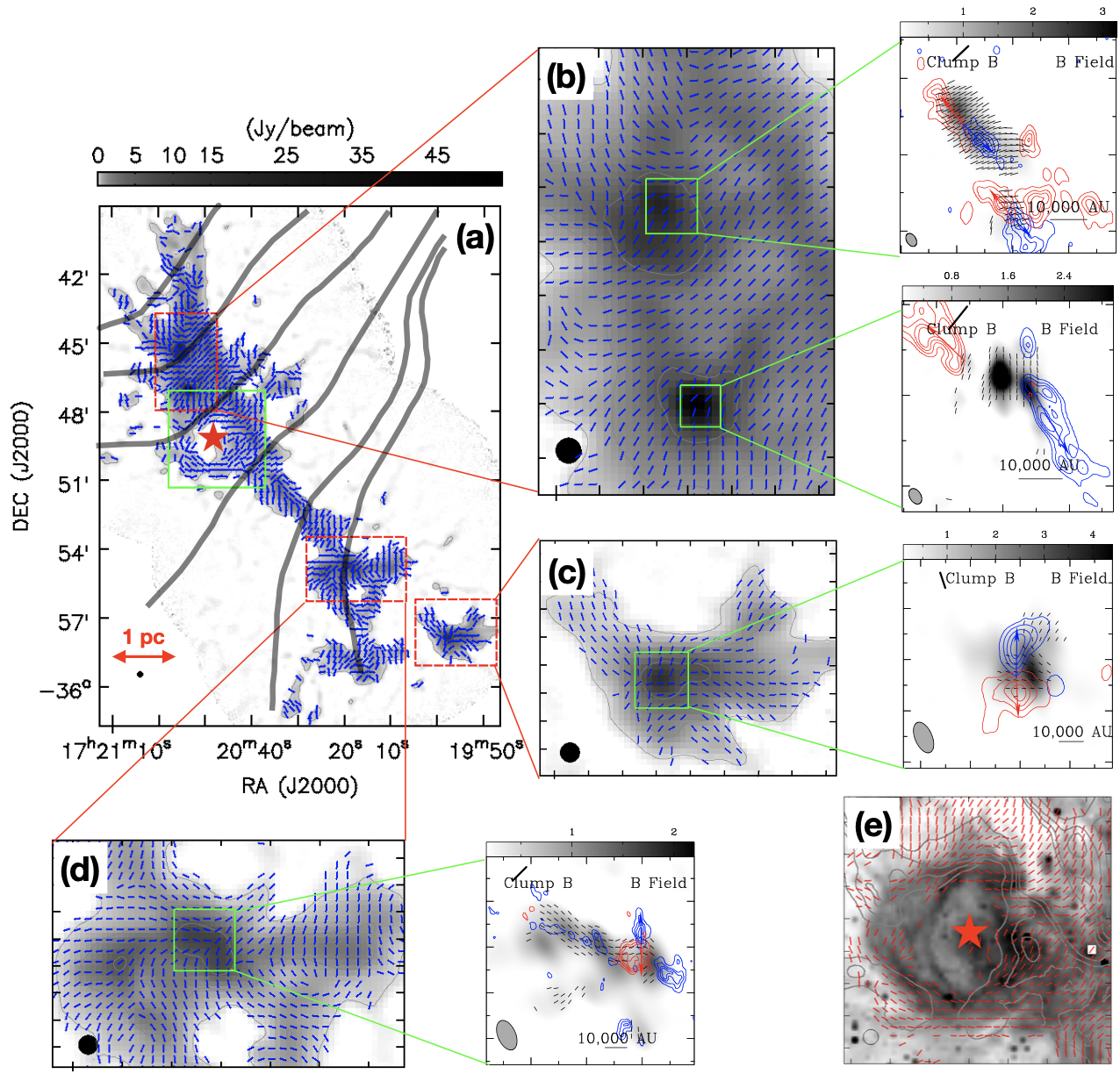
Figure 1: Magnetic fields inside the filamentary cloud NGC 6334. (a) The blue segments show magnetic field orientations obtained with JCMT/POL-2 at 850 $\mu m$ with a pixel size of 12^′′ (Arzoumanian et al., 2021). The background image shows 850 $\mu m$ Stokes I emission. The gray curves show the magnetic field lines inferred from SPARO polarization observations (Li et al., 2015a). (b-d) The blue segments show magnetic field orientations obtained with JCMT/POL-2 at 850 $\mu m$ with a pixel size of 4^′′ (Arzoumanian et al., 2021). The zoom-in aside panels show magnetic field orientations superposed on the Stokes I continuum emission at 345 GHz, observed by SMA at dense core scale (Zhang et al., 2014). The blue and red contours show the high-velocity CO outflow emission (Zhang et al., 2014). (e) Red segments show magnetic field orientations in the region outlined by the green box in panel a. The contours show 850 $\mu m$ Stokes I emission. The contour levels are 0.2, 0.4, 0.6 and 0.8 Jy beam^-1. The red stars in panels a and e represent the Hii region “source II” or “D”. The background image shows the Spitzer/IRAC 3.6 $\mu$m emission, from which the infrared bubble produced by the Hii region is clearly seen. The magnetic fields are reshaped by the Hii region and curved along the compressed shell.

Star formation occurs within clouds of molecular hydrogen, the densest phase of the interstellar medium (ISM). However, the turbulence, magnetization and gravity of the ISM turn star formation into a multi-scale process. Molecular clouds are weakly ionized by UV photons and cosmic rays (McKee and Ostriker, 1977) and, therefore, are coupled to the Galactic magnetic field (Mestel and Spitzer, 1956) at all but the very highest densities in pre-star-formation gas (Caselli et al., 1998). Throughout its volume, the ISM is therefore a magnetised turbulent fluid, in which stars form in the highest-density, gravitationally unstable regions of molecular clouds (e.g., Benson and Myers, 1989). Star formation is not the end-point of the process of ISM evolution; feedback effects from young stars and supernovae play a significant role in molecular cloud evolution and driving ISM turbulence (e.g., Krumholz et al., 2014). Fig. 1 illustrates the ordered magnetic fields that pervade star-forming molecular clouds on all size scales. These magnetic fields can affect the evolution of star-forming regions in many ways: for example by altering the characteristics of turbulence (e.g., Brandenburg and Lazarian, 2013), changing the characteristics of shocks (e.g., Inoue et al., 2009), providing directionality to gas flows (e.g., Soler et al., 2013; Seifried and Walch, 2015), providing pressure support against gravitational instability (e.g., Nakano and Nakamura, 1978), removing angular momentum (e.g., Allen and Burton, 1993), and transporting feedback (e.g., Offner and Liu, 2018) and cosmic rays (e.g., Shukurov et al., 2017) over large scales.

Stars form inefficiently; the Galactic star formation rate is orders of magnitude lower than if clouds were in a state of freefall collapse (e.g., Scalo, 1986), and molecular clouds typically convert only a few percent of their mass into stars (e.g., Leisawitz et al., 1989). Both magnetic fields and turbulence have been invoked as a means of supporting molecular clouds against gravitational collapse. In the past, theories of the role of magnetic fields have tended toward the extremes: star formation either as a secular process mediated by ambipolar diffusion (ion-neutral drift) in a magnetically-dominated ISM (e.g., Shu et al., 1987), or as the result of dynamic cloud evolution driven by supersonic and super-Alfvénic turbulence (e.g., Mac Low and Klessen, 2004). Such disparate models have developed in parallel in large part due to the significant difficulties in measuring interstellar magnetic field morphology and strength (e.g., Crutcher, 2012), and in understanding and modelling the properties of magnetohydrodynamic (MHD) turbulence and so making testable predictions for magnetic field behavior (e.g., Krumholz and Federrath, 2019).

However, a more complete observational and theoretical understanding has emerged over the last decade, thanks to major advances in instrumentation (e.g., Lamarre et al., 2010; Friberg et al., 2016; Cortes et al., 2016) and the frequent inclusion of magnetic fields into simulations of ISM physics (e.g., Vázquez-Semadeni et al., 2011; Seifried and Walch, 2015; Li and Klein, 2019). The increasing community interest in combining our observational and theoretical knowledge is reflected in the direct comparison of theory and observations through production of synthetic observations of simulations (e.g., Soler et al., 2013; Seifried et al., 2019; King et al., 2018).

In this chapter we present a multi-scale review of magnetic fields in star-forming regions, ranging from the formation of giant molecular cloud complexes ($\sim 100$ pc) to dense cores forming individual stellar systems ($\sim 0.01$  pc), focusing in particular on these key questions:
• What are the three-dimensional (3D) morphologies of the magnetic fields of molecular clouds and their substructures, and do the observed field properties agree with different formation models of clouds, filaments and cores?
• Do magnetic fields direct gas accretion onto dense substructures, or are they distorted by gas motions, and how well coupled is the magnetic field to the gas in different density regimes?
• How does the energy balance between magnetic fields, turbulence and gravity change as a function of density and size-scale, and can variations in this balance lead to differences in cloud structure and star formation efficiency?

We first discuss the current state of instrumentation and key metrics and methods for measuring the strength and dynamic importance of magnetic fields in §2. We review magnetic fields in molecular clouds in §3, in dense, star-forming filaments in §4, and in dense molecular cores in §5. In §6 we present a synthesis of these results, revisiting our key questions to discuss our current understanding of how magnetic fields affect the star formation process. Finally, we discuss forthcoming observations and simulations over the next five years, and how these may address the outstanding issues in this rapidly evolving field.

2 MEASUREMENTS, METRICS & METHODS

2.1 Recent advances in instrumentation

In the last decade there have been major advances in polarimetric instrumentation, particularly in the development of far-infrared (FIR) and (sub)millimeter cameras sensitive to polarized dust emission. Perhaps the most important advance has been the $Planck$ satellite (Lamarre et al., 2010), which produced all-sky 353 GHz (850$\mu$m) dust polarization maps (Planck Collaboration VIII, 2015). Significant advances have also been made on the ground: the James Clerk Maxwell Telescope (JCMT)’s POL-2 polarimeter (Friberg et al., 2016) on the SCUBA-2 camera (Holland et al., 2013) operates at 850$\mu$m and 450$\mu$m. The Atacama Pathfinder Experiment (APEX) telescope also offered the PolKa polarimeter at 870$\mu$m (Wiesemeyer et al., 2014). The Atacama Large Millimeter/submillimeter Array (ALMA) has developed polarization capabilities (Cortes et al., 2016; Hull et al., 2020b), while the Submillimeter Array (SMA) has an upgraded correlator (Primiani et al., 2016).

Stratospheric polarimetry is becoming increasingly important, particularly in the absence of any new space-based polarimeters in the intermediate term. The Stratospheric Observatory for Infrared Astronomy (SOFIA)’s HAWC+ camera (Harper et al., 2018) operates in five bands from 53$\mu$m to 214$\mu$m, while the Balloon-borne Large-Aperture Submillimetre Telescope for Polarimetry (BLASTPol; (250$\mu$m, 350$\mu$m, 500$\mu$m) (Galitzki et al., 2014) and PILOT (214$\mu$m) (Foënard et al., 2018) telescopes have flown from different launch sites around the world.

The new large-detector-count cameras on single-dish instruments have made wide-area polarimetric surveys feasible. JCMT/POL-2 and SOFIA/HAWC+ have dedicated surveys of large areas of molecular clouds at resolutions of $\sim 10^{\prime\prime}$ in polarized light (e.g., the JCMT BISTRO Survey; Ward-Thompson et al., 2017). Moreover, optical and near-IR polarimeters have provided detailed large-scale maps of magnetic fields in low-density regions of molecular clouds, including SIRPOL on the InfraRed Survey Facility (IRSF; Kandori et al., 2006), Pico dos Dias (Magalhaes et al., 1996), the ARIES Imaging Polarimeter (AIMPOL) on the Sampurnanand telescope (Rautela et al., 2004), and Mimir on the Perkins Telescope (Clemens et al., 2007, 2020).

2.2 Key ISM magnetic field tracers

2.2.1 Zeeman splitting of spectral lines

Line-of-sight magnetic field strengths can be directly measured through Zeeman splitting of spectral lines of paramagnetic species, observed either in absorption or emission. In species with an unpaired electron, the line shifts induced by the Zeeman effect $\Delta\nu_{z}\propto\mu_{\textsc{b}}B$, where $\mu_{\textsc{b}}$ is the Bohr magneton. The Zeeman effect has been detected in extended gas in Hi, OH and CN. Hi in emission traces the cold neutral medium at hydrogen number densities $\sim 10^{0}-10^{2}$ cm^-3; OH emission and Hi absorption trace a similar range of densities, $\sim 10^{2}-10^{4}$ cm^-3, and CN traces densities $\sim 10^{5}-10^{6}$ cm^-3. The Zeeman effect can in principle give information on both the line-of-sight (LOS) and plane-of-sky (POS) components of the magnetic field ($B_{\textsc{los}}$ and $B_{\textsc{pos}}$ respectively); splitting due to the LOS component is seen in the Stokes $V$ (circular polarization) spectrum, with amplitude $\propto(\Delta\nu_{z}/\sigma_{v})B_{\textsc{los}}$, where $\sigma_{v}$ is the characteristic width of the spectral line, while splitting due to the POS component is seen in the Stokes $Q$ and $U$ (linear polarization) spectra, with amplitude $\propto(\Delta\nu_{z}/\sigma_{v})^{2}B_{\textsc{pos}}$. (See, e.g., Tinbergen 1996 for definitions of the Stokes parameters.) Typically, $\Delta\nu_{z}\ll\sigma_{v}$ and so only the LOS component (and its direction) can be recovered. Detecting the LOS Zeeman effect is itself very observationally intensive and requires Stokes $V$ instrumental polarization to be very well-characterised.

The Zeeman effect is more easily observed in polarized maser emission, which arises from compact (10–100 au) objects with high brightness temperatures and densities (e.g. Crutcher and Kemball, 2019). Maser emission probes the small-scale physics of the later stages of high-mass star formation. Key masing species include OH, associated with ultra-compact HII regions (e.g. Caswell et al., 2011); H₂O, tracing outflow shocks and protostellar discs (e.g. Vlemmings et al., 2006); and CH₃OH, tracing outflow shocks from high-mass star-forming regions (Class I), and the vicinities of massive protostars (Class II) (e.g Cyganowski et al., 2009). The accuracy of magnetic field strength measurements in masing regions is being improved by modelling, including of non-Zeeman maser polarization (Lankhaar and Vlemmings, 2019; Dall’Olio et al., 2020).

The Zeeman effect is a ‘gold standard’ to which indirect measurements of ISM magnetic field strength are typically benchmarked (e.g., Heiles and Robishaw, 2009; Poidevin et al., 2013). Despite this there are some caveats to Zeeman-derived magnetic field strengths: measurements are subject to line-of-sight reversals and beam integration effects (e.g., Poidevin et al., 2013), and the significant time required to make the observations, particularly in higher-density gas traced by CN, mean that measurements at high densities are biased toward high-mass regions (Crutcher et al., 1999; Falgarone et al., 2008). Only a handful of new non-masing Zeeman measurements have been published in the last decade (Pillai et al., 2016; Thompson et al., 2019; Ching et al., 2022).

2.2.2 Faraday rotation

When a linearly polarized electromagnetic (EM) wave passes through a magnetised region that contains free electrons (magnetized plasma), its plane of polarization rotates. This phenomenon is known as Faraday rotation and the amount of rotation can be obtained by:

$$\Delta\psi=\lambda^{2}\big{(}0.812\int{n_{e}\mbox{\boldmath$B$}\cdot\mbox{\boldmath$dl$}}\big{)}=\lambda^{2}\rm{RM},$$ (1)

where $\Delta\psi$ is the amount of rotation (rad), $\lambda$ is the wavelength of the EM wave (m), $n_{e}$ is the electron volume density of the magnetized region (cm^-3), $B$ is the magnetic field strength ($\mu$G), and $dl$ is the path length (pc). The quantity in brackets is the rotation measure (RM; rad m^-2). Faraday rotation occurs because the ISM acts as a birefringent medium in the presence of magnetic fields and free electrons, resulting in different refractive indices for right- and left- circularly polarized EM waves. Faraday rotation provides information about the component of the magnetic field along the LOS. Interstellar synchrotron emission is a source for linearly polarized EM waves.

Traditionally, Faraday rotation of linearly polarized emission from pulsars and extragalactic compact sources was used to study galactic magnetic fields (e.g., Brown et al., 2007; Van Eck et al., 2011) or the magnetic field of strongly ionized regions within the Galaxy (Harvey-Smith et al., 2011). Various RM catalogs are available (e.g, Schnitzeler et al., 2019; Van Eck et al., 2021); currently, the most extensive is that of Taylor et al. (2009), although being made at only two wavelengths, the uncertainty ranges in their derived RM values are relatively high.

Following the development of RM synthesis techniques (Burn, 1966; Brentjens and de Bruyn, 2005), more information could be extracted about the ISM magnetic fields, including cold neutral H$I$1.2ex filaments (e.g., Zaroubi et al., 2015; Van Eck et al., 2019; Bracco et al., 2020b, using Low-Frequency Array, LOFAR, observations) or the foregrounds of H$II$1.2ex regions (Thomson et al., 2019, using the Parkes 64-m Radio Telescope as part of the Global Magneto-Ionic Medium Survey). It was thought that molecular clouds have $\sim$ zero contribution to the RM due to low abundance of free electrons. However, Tahani et al. (2018) showed that a combination of stronger magnetic fields, the presence of free electrons in these regions due to cosmic rays, and higher densities resulting in higher electron densities even with lower ionization fractions, can result in an observable RM in these regions. Even though UV fields can be strongly attenuated in dense molecular clouds, cosmic rays are an important source of ionization in these regions (e.g., Bergin et al., 1999; Everett and Zweibel, 2011; Padovani et al., 2018) and the ionization rates in denser regions can be higher than previously thought (Padovani et al., 2018).

Tahani et al. (2018) developed a new technique using Faraday rotation from extragalactic sources and pulsars to determine the LOS magnetic field component in molecular clouds. This technique exploits an on-off approach to decouple the RM contribution by the cloud from the Galactic contribution (everything along the LOS except the cloud). They then used extinction maps and a chemical evolution code to estimate the electron column densities and so the LOS magnetic field strength. They found that their obtained magnetic field directions were consistent with atomic Zeeman observations in the envelopes of molecular clouds.

2.2.3 Dust extinction/emission polarization

Interstellar dust polarization (Hall, 1949; Hiltner, 1949) in most ISM environments arises from grains aligned with their minor axis parallel to the magnetic field (Davis and Greenstein, 1951), causing preferential polarization of dust-extincted optical and near-infrared (NIR) emission parallel to, and of far-IR and (sub)millimeter dust continuum emission perpendicular to, the POS magnetic field direction. Radiative Alignment Torques (B-RATs; Dolginov and Mitrofanov 1976; Lazarian and Hoang 2007a) is the leading theory of grain alignment, in which paramagnetic grains are spun up by a non-isotropic radiation field to precess around the local magnetic field direction (Andersson et al., 2015)

Dust polarization is a key tool because it allows plane-of-sky magnetic field direction to be traced over large areas and a wide range of densities relatively inexpensively. Polarization fraction is at a maximum of $\sim 0.2$ in the low-density ISM (Planck Collaboration Int. XIX, 2015), and typically decreases significantly with increasing gas column density, to $<0.01$ in starless cores (e.g., Jones et al., 2015). This ‘polarization hole’ effect may be caused by some combination of loss of grain alignment at high visual extinction ($A_{V}$) (e.g., Whittet et al., 2008), integration of complex field geometries within a telescope beam (‘field tangling’) (e.g., Hull et al., 2014), and centrifugal destruction of dust grains by radiative torques in the immediate vicinity of protostars (‘radiative torque disruption’, RATD; Hoang et al. 2019). Interferometric observations of protostellar systems show that grains can remain aligned (e.g., Kwon et al. 2019), but in these sources there is an internal source of photons to drive grain alignment. Observations of the starless core FeST 1-457 have suggested that grains are unaligned beyond $A_{V}\sim 20-30$ mag (Alves et al., 2014; Jones et al., 2015); however, externally-illuminated starless cores may retain some degree of grain alignment to high $A_{V}$ (Pattle et al., 2019). Hoang et al. (2021) proposed an analytical model in which the maximum $A_{V}$ at which grains remain aligned varies as a function of incident radiation anisotropy, gas density and grain size, among other parameters, with larger grains remaining aligned to significantly higher $A_{V}$.

2.2.4 Goldreich-Kylafis effect

Emission line polarization can arise from the Goldreich-Kylafis (GK) effect (Goldreich and Kylafis, 1981), in which molecular line emission may be linearly polarized either parallel or perpendicular to the plane-of-sky magnetic field. The GK effect, which can provide a velocity-resolved probe of magnetic field morphology, has been observed in outflows (e.g. Girart et al., 1999; Ching et al., 2017), and in the high-mass star-forming region NGC6334I(N) using ALMA (Cortes et al., 2021a). However, the uncertainty on polarization direction complicates interpretation. ALMA’s ability to measure both line and continuum polarization in a single spectral set-up will be key to understanding under what conditions the GK effect produces parallel or perpendicular alignment (e.g. Cortes et al., 2021a). A further complication is conversion of linear to circular line polarization by anisotropic resonant scattering by foreground material (Houde et al., 2013; Chamma et al., 2018).

2.2.5 Velocity gradients

The Velocity Gradient Technique (VGT; González-Casanova and Lazarian 2017), is a new method for inferring magnetic field morphologies, primarily in the low-density ISM. VGT makes use of the elongation of turbulent eddies in the ISM along the local magnetic field direction, positing that fast turbulent magnetic reconnection across these eddies results in turbulent fluid motions being preferentially perpendicular to the magnetic field. Tests against simulations suggest that an optically thin gas tracer can be used to trace magnetic fields in regions with supersonic, trans- and sub-Alfvénic turbulence and without strong gravitational collapse (Hsieh et al., 2019), and the method has reproduced the large-scale magnetic field morphology of nearby GMCs with reasonable accuracy (Hu et al., 2019).

VGT assumes that the velocity gradients seen in thin channel maps are associated with turbulent rather than density structures (González-Casanova and Lazarian, 2017). However, Hi structures in the diffuse ISM have been shown to be associated with density enhancements (Clark et al., 2019). A striking alignment between velocity gradients and magnetic field directions is seen in the low-density, non-self-gravitating ISM, but debate continues over the physical origin of this effect (e.g., Kalberla et al., 2020). A major strength of VGT is that it is velocity-resolved, probing the magnetic field structures of multiple velocity components along a single LOS (e.g., Hu et al., 2019). Moreover, where the assumptions of VGT break down may be a good probe of the transition of the ISM to the gravity-dominated regime (cf. Hu et al., 2020, 2021), and VGT could be used to make predictions for where this transition occurs.

2.3 Metrics and methods

2.3.1 Key metrics

We here outline the key metrics by which the relative importance of magnetic fields in the ISM is parameterized, the values of which may change with size and density scale.

Energy balance Magnetic energy is given by

$$E_{B}=\frac{B^{2}V}{2\mu_{0}}\,\,({\rm SI})=\frac{B^{2}V}{8\pi}\,\,({\rm cgs}),$$ (2)

where $V$ is volume, and can be compared to the other energy terms, typically gravitational potential energy, thermal or non-thermal kinetic energy and external pressure energy. $E_{B}$ is typically subject to large uncertainties.

Mass-to-flux ratio The critical mass-to-flux ratio is

$$\left(\frac{M}{\Phi}\right)_{crit}=\frac{1}{2\pi\sqrt{G}}\,\,{\rm(cgs)},$$ (3)

(Nakano and Nakamura, 1978). The mass-to-flux ratio is then given in units of the critical value by

$$\mu_{\Phi}=\frac{(M/\Phi)}{(M/\Phi)_{crit}}=2\pi\sqrt{G}\mu m_{\textsc{h}}\left(\frac{N}{B}\right)\,\,{\rm(cgs)},$$ (4)

where $N$ is column density, $B$ is magnetic field strength, and $\mu$ is mean molecular weight. A value $\mu_{\Phi}>1$ indicates that the region is magnetically supercritical, i.e. the magnetic field cannot prevent gravitational collapse, while $\mu_{\Phi}<1$ indicates that the region is magnetically subcritical, i.e. magnetically supported. Geometric corrections to $\mu_{\Phi}$ can be significant (Crutcher et al., 2004).

Alfvén Mach number The Alfvén velocity,

$$v_{A}=\frac{B}{\sqrt{\mu_{0}\rho}}\,\,({\rm SI})=\frac{B}{\sqrt{4\pi\rho}}\,\,({\rm cgs}),$$ (5)

where $\rho$ is gas density and $\mu_{0}$ is the permeability of free space, is the group velocity of transverse oscillations of matter and magnetic field lines, for which magnetic tension is the restoring force. This must be measured across magnetic field lines; $v_{A}$ along a field line is infinite. The relative importance of magnetism and non-thermal gas motions is parameterised by the Alfvén Mach number,

$$\mathcal{M}_{A}=\frac{\sigma_{v,\textsc{nt}}}{v_{A}}\propto\left(\frac{E_{K,\textsc{nt}}}{E_{B}}\right)^{0.5},$$ (6)

where $\sigma_{v,\textsc{nt}}$ is the non-thermal velocity dispersion, $E_{B}$ is magnetic energy and $E_{K,\textsc{nt}}$ is non-thermal kinetic energy. If turbulence is isotropic then $\sigma_{v,\textsc{nt}}$ should be 3D, i.e. $\sqrt{3}\times$ its measured LOS value (Crutcher et al., 1999). However, turbulence will be anisotropic in the presence of a strong mean magnetic field. $\mathcal{M}_{A}<1$ (sub-Alfvénic) indicates that magnetic fields direct gas motions; $\mathcal{M}_{A}>1$ (super-Alfvénic) indicates the converse. $\mathcal{M}_{A}$ is analogous to sonic Mach number, $\mathcal{M}=\sigma_{v,\textsc{nt}}/c_{s}$, where $c_{s}$ is sound speed.

Plasma beta The thermal-to-magnetic pressure ratio is

$$\beta=\frac{nk_{\textsc{b}}T}{B^{2}/2\mu_{0}}\,\,({\rm SI})=\frac{nk_{\textsc{b}}T}{B^{2}/8\pi}\,\,({\rm cgs})=\frac{E_{K,\textsc{t}}}{E_{B}},$$ (7)

where $T$ is temperature, $n$ is number density, and $E_{K,\textsc{t}}$ is thermal kinetic energy. A value of $\beta\ll 1$ indicates a magnetically-dominated system; $\beta\gg 1$ indicates a thermally-dominated system.

Jeans Mass The classic measure of stability of an isothermal gas sphere is the Jeans mass (Jeans, 1928),

$$M_{J}=\frac{4\pi}{3}\frac{c_{s}^{3}}{G^{3/2}\rho^{1/2}}.$$ (8)

If non-thermal motions are taken to represent an effectively hydrostatic pressure against collapse (the microturbulent assumption, Chandrasekhar 1951), then $c_{s}$ can be replaced by $\sigma_{v,\textsc{nt}}$ or $(c_{s}^{2}+\sigma^{2}_{v,\textsc{nt}})^{0.5}$. A structure with a mass significantly greater than its Jeans mass is suggestive of significant magnetic support (e.g., Sanhueza et al. 2019).

Virial balance The overall energetic balance of a small-scale cloud structure can be estimated in terms of its virial balance; however, this makes the assumption, invalid except on scales smaller than the thermal Jeans wavelength, $\lambda_{J}=c_{s}(\pi/G\rho)^{0.5}$, that the structure is evolving quasistatically, with turbulent motions providing mean support against gravity (Mac Low and Klessen, 2004).

Freefall time An ISM structure in a state of unimpeded gravitational collapse will collapse on its freefall timescale,

$$t_{ff}=\left(\frac{3\pi}{32G\rho}\right)^{0.5}.$$ (9)

Ambipolar diffusion timescale A structure evolving quasistatically to instability in a strong magnetic field will have a lifetime set by the ambipolar diffusion timescale – the characteristic timescale of magnetic flux loss as neutral species drift past ions (e.g., Heitsch and Zweibel, 2003):

$$t_{AD}=\frac{L^{2}}{\lambda_{AD}},$$ (10)

where $L$ is the characteristic size of the structure in question and $\lambda_{AD}$ is the ambipolar diffusivity,

$$\lambda_{AD}=\frac{\mu_{i}+\mu_{n}}{4\pi\langle\sigma v\rangle\mu_{i}\mu_{n}m_{\textsc{h}}x_{i}}\left(\frac{B}{n_{n}}\right)^{2}\,\,{\rm(cgs)},$$ (11)

where $\mu_{i}$ and $\mu_{n}$ are the mean molecular weight of ions and neutrals respectively, $n_{n}$ is the number density of neutrals, $x_{i}$ is ionization fraction, and $\langle\sigma v\rangle$ is the rate coefficient for elastic collisions ($\langle\sigma v\rangle=1.5\times 10^{-9}\,$cm³s^-1; Draine et al. 1983). Various formulations of $t_{AD}$ exist for the dense, cosmic-ray-ionized ISM, many of which assume ionization-recombination balance, and so that

$$x_{i}\propto\left(\frac{n_{n}}{\zeta}\right)^{-0.5}\approx 1.2\times 10^{-5}n_{n}^{-0.5}\,\,({\rm cgs}),$$ (12)

where $\zeta$ is cosmic ray ionization rate (Elmegreen, 1979; Umebayashi and Nakano, 1980). A recent formulation of $t_{AD}$ (Heitsch and Hartmann, 2014) is

$$t_{AD}=1.38\times 10^{3}\left(\frac{L}{1\,{\rm pc}}\right)^{2}\left(\frac{n}{300\,{\rm cm}^{-3}}\right)^{1.5}\left(\frac{B}{5\,\mu{\rm G}}\right)^{-2}\,\,{\rm Myr}.$$ (13)

Magnetic field-density relation The relationship between $B$ and $n$ is typically parameterised as

$$B\propto n^{\kappa}.$$ (14)

Collapse of a spherical cloud with flux-freezing should produce $\kappa\approx 2/3$ (Mestel, 1966), while ambipolar diffusion models predict $0<\kappa<0.5$, evolving from $\kappa\sim 0$ initially (indicating collapse along field lines) to $\kappa\sim 0.5$ in the later stages of collapse (indicating collapse across field lines) (e.g., Mouschovias and Ciolek, 1999). $\kappa>0$ indicates that magnetic flux is increasing with density (e.g., Tritsis et al., 2015), and so that the field is being compressed, typically by gravity, although stellar feedback in Hii regions could also cause such compression. A widely used form of eq. 14, following Crutcher et al. (2010), is

$$B=\begin{cases}B_{0}&(n<n_{0})\\ B_{0}\left(\dfrac{n}{n_{0}}\right)^{\kappa}&(n>n_{0})\end{cases}.$$ (15)

2.3.2 The Davis-Chandrasekhar-Fermi (DCF) method

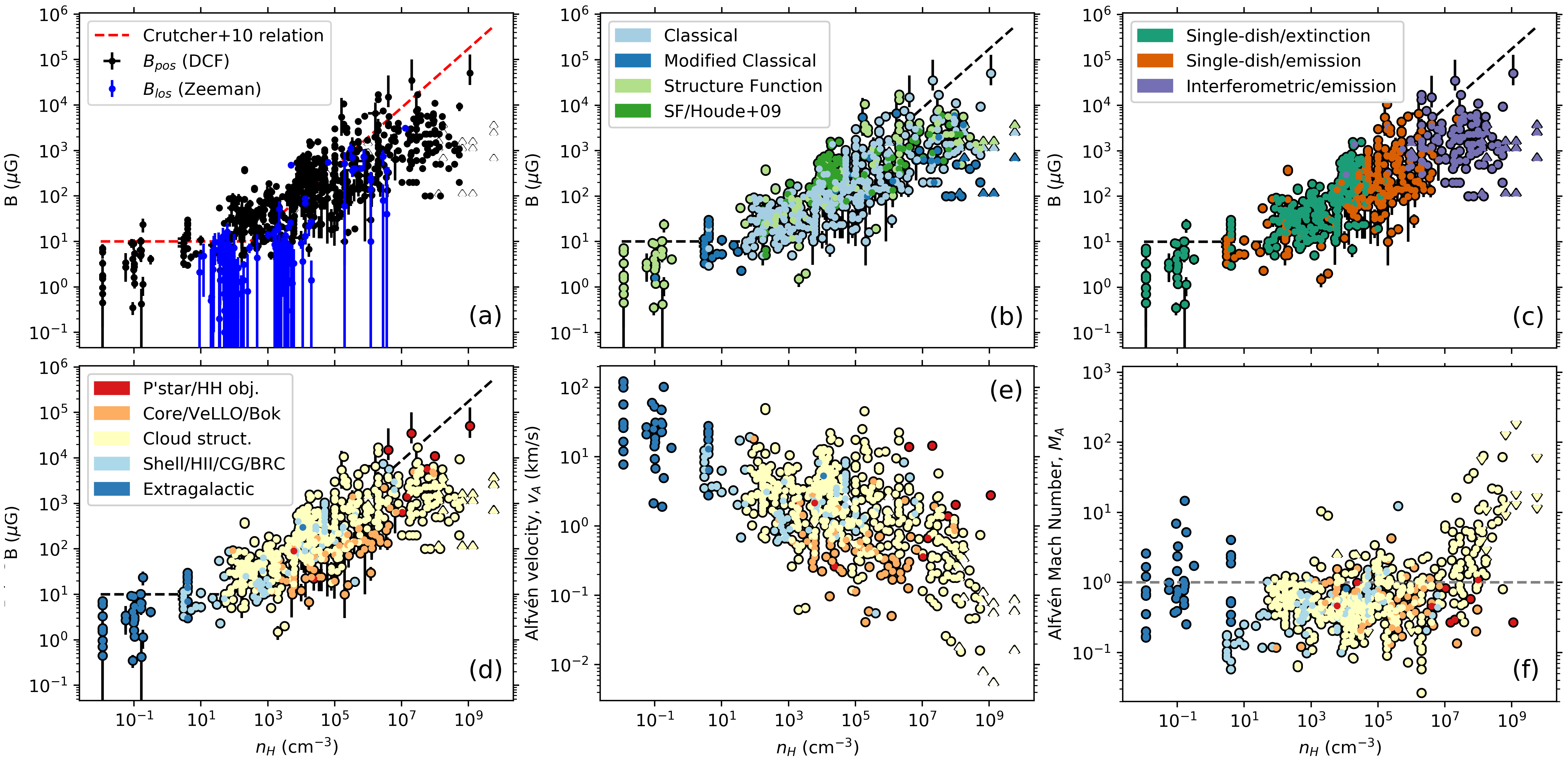
Figure 2: (a): magnetic field strength as a function of hydrogen number density: black points show DCF measurements; blue show Zeeman measurements. Arrows show upper/lower-limit measurements. Red dashed line shows the Crutcher et al. (2010) relation. (b): as (a), but with DCF measurements only. Data points are color-coded by DCF variant. (c): as (b), color-coded by measurement type. (d): as (b), color-coded by object type. (e): Alfvén velocity of the DCF measurements, color-coded by object type. (f): Alfvén Mach number of the DCF measurements, color-coded by object type. Dashed line marks $\mathcal{M}_{A}=1$. References: Alina et al. (2020), Alves et al. (2008, 2011), Andersson and Potter (2005, 2006), Añez-López et al. (2020), Arzoumanian et al. (2021), Attard et al. (2009), Beltrán et al. (2019), Bertrang et al. (2014), Beuther et al. (2010, 2018), Cashman and Clemens (2014), Chakraborty and Das (2016), Chapman et al. (2011), H.-R. Chen et al. (2012a), Z. Chen et al. (2012b; 2017), Ching et al. (2017), Choudhury et al. (2019), Chuss et al. (2019), Cortes and Crutcher (2006); Cortes et al. (2010, 2016, 2019); Cortes et al. (2021b), Coudé et al. (2019), Crutcher et al. (2004), Curran et al. (2004); Curran and Chrysostomou (2007), Dall’Olio et al. (2019), Das et al. (2016), Devaraj et al. (2021), Dewangan et al. (2015, 2018), Eswaraiah et al. (2013, 2017, 2019, 2020, 2021), Franco and Alves (2015), Frau et al. (2014), Girart et al. (2006), Henning et al. (2001), Heyer et al. (2008), Hildebrand et al. (2009), Hily-Blant and Falgarone (2007), Houde et al. (2009, 2016), Hoq et al. (2017), Hull et al. (2017), Joubaud et al. (2019), Juárez et al. (2017), Kandori et al. (2017b, 2020f, 2020d, 2020b, 2020e, 2020a), Karoly et al. (2020), Kim et al. (2016), Kirby (2009), Kirk et al. (2006), Könyves et al. (2021), Kusune et al. (2015, 2016), J. Kwon et al. (2010; 2011; 2016; 2018), W. Kwon et al. (2019), Lada et al. (2004), Lai et al. (2001, 2002), Lee et al. (2014, 2018), Li and Henning (2011); Li et al. (2015a), J. Liu et al. (2019; 2020), T. Liu et al. (2018a; 2018b), Lobo Gomes et al. (2015), Mao et al. (2008), Marchwinski et al. (2012), Matthews et al. (2002, 2005), Neha et al. (2016, 2018), Ngoc et al. (2021), Palau et al. (2021), Panopoulou et al. (2016), Pattle et al. (2017, 2018); Pattle et al. (2021a), Pereyra and Magalhães (2007), Pillai et al. (2015, 2016), Planck Collaboration et al. (2016c), Poidevin and Bastien (2006); Poidevin et al. (2013), Qiu et al. (2013, 2014), Rao et al. (2009), Rathborne et al. (2009), Redaelli et al. (2019), Rodrigues et al. (2007), Sadavoy et al. (2018), Santos et al. (2014, 2016), Sharma et al. (2020), Soam et al. (2015a, b, 2017a, 2017b, 2018b, 2018a, 2019b, 2019a); Soam (2021), Soler et al. (2018), Stephens et al. (2013), Sugitani et al. (2010, 2011, 2019), Tamaoki et al. (2019), Tang et al. (2009, 2019), Tsuboi et al. (2021), Vallée et al. (2003); Vallée and Fiege (2005, 2006, 2007a, 2007b); Vallée (2007), Wang et al. (2019); Wang et al. (2020a), Wisniewski et al. (2007), Wolf et al. (2003), Wright et al. (2014), Zielinski et al. (2021).

The Davis-Chandrasekhar-Fermi (DCF) method (Davis, 1951; Chandrasekhar and Fermi, 1953a) is a means of estimating $B_{\textsc{pos}}$ by taking dispersion in polarization angle from dust emission or extinction measurements to indicate distortion of the magnetic field by non-thermal gas motions, and so to be a measure of $\mathcal{M}_{A}$. For a given turbulent velocity dispersion and gas density, magnetic field strength can then be inferred. The DCF equation in its original form is

$$B_{\textsc{pos}}=\sqrt{\mu_{0}\rho}\frac{\sigma_{v,\textsc{nt}}}{\sigma_{\theta}}\,\,({\rm SI})=\sqrt{4\pi\rho}\frac{\sigma_{v,\textsc{nt}}}{\sigma_{\theta}}\,\,({\rm cgs})$$ (16)

where $\rho$ is gas density, $\sigma_{v,\textsc{nt}}$ is non-thermal linewidth in a gas species taken to trace the same material as the dust polarization observations, and $\sigma_{\theta}$ is dispersion in polarization position angle. DCF makes several assumptions, most notably that turbulence is sub-Alfvénic, but also that the underlying magnetic field geometry is linear, and that $\sigma_{v,\textsc{nt}}$ traces turbulent motions. Nonetheless, it provides an estimation of magnetic field strength from dust polarization, and so is widely used despite long-standing theoretical concerns (e.g., Zweibel, 1990; Myers and Goodman, 1991; Houde et al., 2009). DCF measures an average $B_{\textsc{pos}}$ in the area over which $\sigma_{\theta}$ is measured; however, recent wide-area high-resolution polarimetric mapping of molecular clouds has led to resolved DCF being used to map $B_{\textsc{pos}}$ variation across clouds (Guerra et al., 2021; Hwang et al., 2021).

The original DCF method likely overestimates $B_{\textsc{pos}}$ due to integration of ordered structure on scales smaller than the telescope beam, and from multiple turbulent cells within the beam and along the LOS (e.g., Ostriker et al., 2001; Houde et al., 2009). We outline the methods of accounting for this here; see Pattle and Fissel (2019) for a detailed comparison.

‘Classical’ DCF modifies eq. 16 by a factor $0<Q\leq 1$, generally $Q=0.5$, such that $(1/\sigma_{\theta})\to(Q/\sigma_{\theta})$ to account for integration effects (Ostriker et al., 2001; Heitsch et al., 2001; Padoan et al., 2001). Cho and Yoo (2016) proposed the ratio of velocity centroid dispersion to linewidth as an estimator of the number of turbulent cells along the LOS. Further modifications can be made to account for large-scale magnetic field structure when estimating $\sigma_{\theta}$ (Pillai et al., 2015; Pattle et al., 2017). Classical DCF is often restricted to regions where $\sigma_{\theta}<25^{\circ}$ (Heitsch et al., 2001).

Alternatively, $\sigma_{v,\textsc{nt}}/\sigma_{\theta}$ in eq. 16 can be replaced with the ratio of energies in the turbulent and ordered field components, such that $1/\sigma_{\theta}\to(\langle B_{t}^{2}\rangle/\langle B_{o}^{2}\rangle)^{-0.5}$. This ratio is determined from the structure function of the dispersion in polarization angles (Falceta-Gonçalves et al., 2008); Hildebrand et al. (2009) proposed a means of accounting for large-scale field structure, and Houde et al. (2009) further expanded the method to account for sub-beam and LOS effects. Lazarian et al. (2020) have recently proposed a variation using structure functions to also measure $\sigma_{v,\textsc{nt}}$.

The proliferation of DCF measurements in recent years has led to renewed interest in testing DCF variants against simulations. Skalidis and Tassis (2021) have proposed an alternative DCF equation, taking non-Alfvénic (compressible) modes to dominate Alfvénic (incompressible) modes,

$$B_{\textsc{pos}}=\sqrt{2\pi\rho}\frac{\sigma_{v,\textsc{nt}}}{\sqrt{\sigma_{\theta}}}\,\,({\rm cgs}),$$ (17)

tested against a range of ideal-MHD simulations by (Skalidis et al., 2021). However, Li et al. (2021) argue that while the compressible modes are significant, compressions and rarefactions largely cancel one another out. Li et al. (2021) present a derivation of, and through comparison with simulations advocate, replacement of $\sigma_{\theta}\to\tan\sigma_{\theta}$ in eq. 16 (cf. Heitsch et al. 2001; Falceta-Gonçalves et al. 2008), thereby removing the small-angle restrictions on classical DCF.

Liu et al. (2021a) applied DCF to simulations, finding that $B_{\textsc{pos}}$ is accurately recovered in strong-field cases, but may be significantly overestimated in super-Alfvénic environments. They propose an environment-dependent $Q$ range, and find that structure functions can characterize ordered field structure and sub-beam integration effects, but that the Cho and Yoo (2016) method may best estimate LOS turbulent cells, with DCF unreliable on size scales $<0.1$ pc unless LOS integration is accounted for. These results encapsulate the challenge of DCF: how its applicability can be judged without an independent measure of $\mathcal{M}_{A}$.

2.3.3 Compilation of literature DCF field strengths

Over the last few years, hundreds of DCF measurements have been published. We have attempted to compile every DCF measurement published since the Ostriker et al. (2001), Padoan et al. (2001) and Heitsch et al. (2001) papers with clearly identifiable density and non-thermal velocity dispersion values. These are shown in Fig. 2a, alongside the Crutcher et al. (2010) Zeeman measurements. There is a striking correlation between the two data sets; the DCF $B_{\textsc{pos}}$ estimates, while typically larger than the Zeeman $B_{\textsc{los}}$ measurements at a given density, are largely compatible with the $B\propto n^{0.65}$ relationship up to densities $\sim 10^{7}$ cm^-3, and then become more broadly distributed.

We classified each measurement as ‘classical’ (using eq. 16 modified by a factor $0<Q\leq 1$), ‘modified classical’ (classical DCF modified following Heitsch et al. 2001; Pillai et al. 2015; Pattle et al. 2017; Cho and Yoo 2016), ‘structure function’ (following Falceta-Gonçalves et al. 2008 or Hildebrand et al. 2009) or ‘SF/Houde+09’ (following Houde et al. 2009), as shown in Fig. 2b. We classified each measurement as arising from either extinction, single-dish emission, or interferometric emission polarimetry, as shown in Fig. 2c. We identified five categories of object: (1) protostar, jet or Herbig Haro object, (2) isolated starless or protostellar core, VeLLO or Bok globule, (3) ‘cloud structure’, any GMC or structure within a GMC, including filaments, clumps and massive dense cores, (4) distinct structures under stellar feedback: shells, Hii regions, cometary globules and bright-rimmed clouds, and (5) extragalactic structures, as shown in Figs. 2d-f.

For DCF measurements the $n$ and $B_{\textsc{pos}}$ axes are not independent (cf. eq. 16), and so it is unsurprising that the results in Fig. 2a-d show a strong correlation. The fundamental quantity being measured in DCF analysis is $\mathcal{M}_{A}$, and so we have attempted to recover this quantity for the measurements in our sample. We calculated $v_{A}=B/\sqrt{4\pi\rho}$, assuming $\rho=\mu m_{\textsc{h}}n_{\textsc{h}}$, and taking a mean particle weight $\mu=2.8$ for molecular gas and 1.4 for atomic gas, as shown in Fig. 2e (calculated from $B_{\textsc{pos}}$ only). We then calculated $\mathcal{M}_{A}=\sigma_{v,\textsc{nt}}/v_{A}$ $=\sigma_{\theta}/Q\,\,{\rm(classical)}=(\langle B_{t}^{2}\rangle/\langle B_{o}^{2}\rangle)^{0.5}\,\,{\rm(s.f.)}$, as shown in Fig. 2f. $\mathcal{M}_{A}$ is broadly flat below $n_{\textsc{h}}\sim 10^{7}$ cm^-3, albeit with scatter in the range 0.1–10. The maximum $\mathcal{M}_{A}$ increases significantly at high densities. The mean value of $\mathcal{M}_{A}$ below $10^{7}$ cm^-3 is 0.74, and the median is 0.52 (again calculated from $B_{\textsc{p}os}$ only), suggesting that turbulence is typically slightly sub-Alfvénic. However, DCF assumes sub-Alfvénic turbulence and so it is unsurprising that we generally recover $\mathcal{M}_{A}<1$.

We discuss this compilation further in §6.1.1. As the analysis which we can perform in this chapter is very limited, we have made this data set available as a resource. We draw attention to a recent analysis of a compilation of emission DCF measurements by Liu et al. (2021b).

2.3.4 The Histogram of Relative Orientations (HRO)

The HRO is commonly used in numerical and observational data to measure the alignment between density or column density structures and the local magnetic field (Soler et al., 2013). The method calculates the angle $\phi$ between the local magnetic field and density gradient and its distribution in different density or column density bins. The scale-dependent behavior of the angle is expressed by an alignment parameter, which is positive (negative) when the magnetic field is predominantly parallel (perpendicular) to the density structures at a given bin. Two commonly used parameters are the HRO shape parameter $\xi=(A_{c}-A_{e})/(A_{c}+A_{e})$, where $A_{c}$ and $A_{e}$ are the number of measurements with $|\phi|\leq 22.5^{\circ}$ and $|\phi|\geq 67.5^{\circ}$ respectively, and the projected Rayleigh statistic $Z_{x}=\sum_{i}^{n}cos(2\phi_{i})/\sqrt{n/2}$ (Jow et al., 2018). The HRO can thus condense the statistical behavior of MHD turbulence into a single parameter, making the method particularly attractive for characterizing molecular clouds.

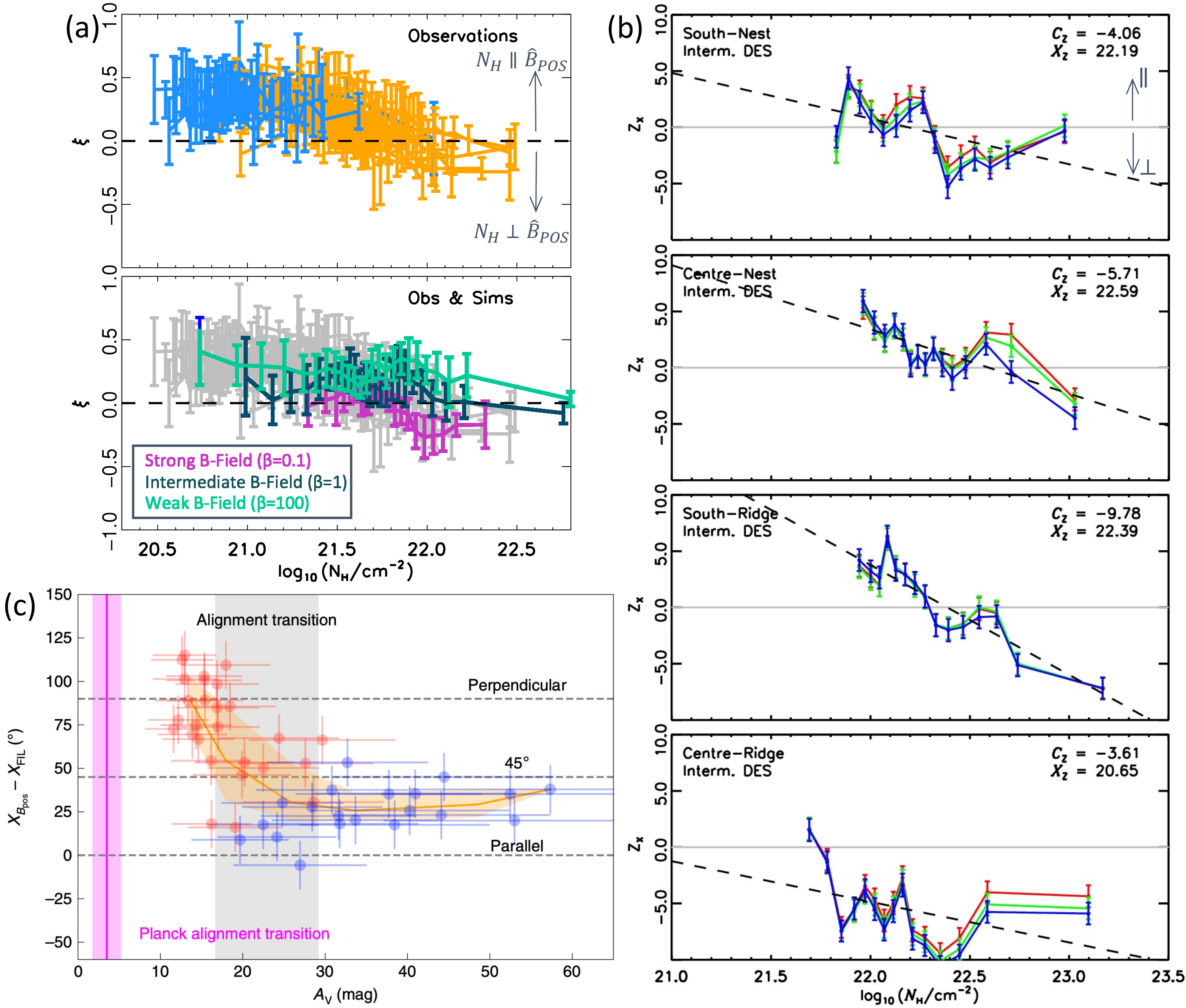
Figure 3: Observations of the relative alignment of cloud column density sub-structure with the magnetic field inferred from dust polarization maps. (a) Comparison of the HRO shape parameter $\xi$ for Planck 10^′ FWHM 353 GHz polarization observations of low column density clouds (blue) and a compilation of higher column density star-forming molecular clouds (orange), bottom panel: Planck $\xi$ vs. $\log(N_{\mathrm{H}})$ observations (gray), compared to the $\xi$ vs. $\log(N_{\mathrm{H}})$ found in simulations from Soler et al. (2013) (adapted from Planck Collaboration et al. 2016c; reproduced with permission © ESO); (b) Relative alignment between Herschel-derived column density maps and BLASTPol 3-color polarization $\hat{B}_{\textsc{pos}}$ maps (red: 500 $\mu$m, green 350 $\mu$m, blue 350 $\mu$m), characterized by the Projected Rayleigh Statistic $Z_{\mathrm{x}}$ vs $\log(N_{\mathrm{H}})$ for four sub-regions of the Vela C cloud (Soler et al., 2017; Jow et al., 2018, Fig. 5; MNRAS 474 1018). The dashed lines show linear fits to $Z_{\mathrm{x}}=C_{\mathrm{Z}}[\log_{10}(N_{\mathrm{H}}/cm^{-2})-X_{\mathrm{Z}}]$; (c) Distribution of relative orientations of the gas filament with respect to $\hat{B}_{\textsc{pos}}$ as a function of $A_{V}$ in the Serpens South cloud (Pillai et al., 2020). The NIR $\hat{B}_{\textsc{pos}}$ are shown as red filled circles and the FIR as blue filled circles. The magenta bar represents the lower $A_{V}$, first alignment transition suggested by Planck data, for the parallel-to-perpendicular transition near $A_{V}\sim$3.5 mag.

HROs indicate that the orientation between density structures in the ISM and the local magnetic field follows a bimodal distribution: below a certain column density, structures preferentially align parallel to the field, and above it, they are perpendicular to it (e.g., Planck Collaboration et al. 2016c, see also Fig. 3). This observation points to a potential metric for the magnetic field strength with respect to gravity and turbulence, discussed in detail in §6.1.3.

2.3.5 Intensity gradients

The intensity gradient method (Koch et al., 2012a, b; Koch et al., 2013) estimates magnetic field strength from the measured angle between the magnetic field direction and the gradient in emission intensity, assumed to be representative of the resultant direction of motion of material due to magnetic, pressure and gravitational forces. This method provides a point-to-point estimate of both ratio of magnetic to gravitional and pressure energy and magnetic field strength, and can be applied to any measure of plane-of-sky magnetic field direction. This method is applicable only where self-gravity is important (Koch et al., 2012a), but in these environments can probe possible evolution of the relative orientation of field/cloud structures (e.g. Koch et al., 2014), and the flow of material within filamentary structures (e.g. Añez-López et al., 2020; Wang et al., 2020a).

2.3.6 Inclination angle

A challenge in studying the magnetic field properties of individual sources is that tracers are usually sensitive to either $B_{\textsc{los}}$ (e.g., Zeeman splitting, Faraday rotation), or POS field morphology (dust polarization, velocity gradients), but not both. For a large sample of objects with a random distribution of 3D magnetic field angles, the mean total magnetic field strength $\langle B\rangle=2\langle B_{\textsc{los}}\rangle$. However, for individual $B_{\textsc{los}}$ measurements, only a lower limit on $B$ can be set.

Magnetic field inclination angles also complicate the interpretation of dust polarization observations. Clouds with weak magnetic fields tend to have less ordered field morphology (e.g. Ostriker et al. 2001; Soler et al. 2013, and §2.3.2), and lower polarization levels due to signal cancellation as the polarization angle changes within the volume probed by a given sightline. However, these observations are also consistent with viewing a more strongly magnetized cloud from an angle nearly parallel to the mean field direction (King et al., 2018), as any small variations in field direction would appear much larger when projected on the POS, while the polarization levels will be lower. It is thus difficult to determine whether a cloud has a weak magnetic field or is viewed from a geometry where $\gamma$, the inclination angle of the magnetic field with respect to the POS, is large.

Some studies have incorporated statistical methods such as Monte Carlo simulations and $\chi^{2}$ analysis to observations of both POS magnetic field morphology and measurements of $B_{\textsc{los}}$ to model the 3D morphology of magnetic fields (Tahani et al., 2019). However this is complicated by the fact that different tracers are sensitive to the field in gas at different ranges of densities and gas phases, so each tracer may have individual biases (see, e.g., §6.1.1).

Chen et al. (2019) developed a method to estimate the mean magnetic field inclination angle from polarized dust emission. Spinning grains with their long axes perfectly perpendicular to the magnetic field should show no projected elongation if viewed parallel to the field ($\gamma\,=\,90^{\circ}$) and so no polarization (Hildebrand, 1988). The projected grain elongation will be maximized when the field is in the POS ($\gamma=0^{\circ}$). If there are no variations in $\hat{B}_{\mathrm{POS}}$, or $\gamma$ along the LOS then measured fractional polarization $p$ is

$$p\,=\,\frac{p_{0}cos^{2}\gamma}{1-p_{0}\left(cos^{2}\gamma-\frac{2}{3}\right)},$$ (18)

where $p_{0}$ is the intrinsic fractional polarization (assumed to be constant within the cloud). $p_{0}$ can be estimated from the maximum $p$ observed in the cloud

$$p_{\mathrm{max}}\,=\,\frac{p_{0}}{1-\frac{1}{3}p_{0}}.$$ (19)

Using Monte Carlo and synthetic observations of MHD simulations Chen et al. (2019) show that estimates of the mean density weighted inclination angle $\hat{\gamma}^{2D}$ from eq. 18 are biased towards intermediate $\gamma$. They derived numerical correction factors from Athena MHD colliding flow simulations that can estimate of $\hat{\gamma}^{2D}$ to within 10–30^∘ accuracy. Sullivan et al. (2021) applied this method to nine polarization maps of molecular clouds from Planck and BLASTPol and found $\langle\gamma\rangle$ ranging from 16^∘ (Musca/Chamaeleon), to 69^∘ (Perseus). Additional numerical and observational studies are needed to determine whether similar methods of estimating $\gamma$ can be applied to low resolution data, to both super- and sub-Alfvénic clouds, and to clouds with variations in dust temperature and grain alignment efficiency.

2.3.7 Ion-to-neutral linewidth ratio

Houde et al. (2000a, b) showed that in molecular clouds, the linewidths of coexisting ions and neutrals differ in the presence of strong magnetic fields. Two effects are posited to cause this difference: firstly, that neutral linewidths trace turbulence, while narrower ion linewidths trace gyromagnetic motion around field lines. This difference may be used to probe 3D magnetic fields by determining the inclination angle $\gamma$ which, combined with Zeeman and dust polarization observations, can describe the 3D field (Houde et al., 2002, 2004).

Alternatively, Li and Houde (2008) suggest that the narrower ion linewidth is due to the differing turbulent velocity dispersion spectra of neutrals and ions below the ambipolar diffusion size scale. They propose

$$B_{pos}=\left[\frac{L^{\prime}}{0.5\,{\rm mpc}}\frac{\sigma_{v,\textsc{nt},n}}{1\,{\rm km\,s}^{-1}}\left(\frac{n_{n}}{10^{6}\,{\rm cm^{-3}}}\right)^{2}\frac{x_{i}}{10^{-7}}\right]^{\frac{1}{2}}\,{\rm mG},$$ (20)

where $L^{\prime}$ is the ambipolar diffusion size scale, at which ions and neutrals decouple (cf. eq. 11), and $\sigma_{v,\textsc{nt},n}$ is measured at $L^{\prime}$. This method has been used to measure field strengths in dense regions (Hezareh et al., 2010; Tang et al., 2018). However, recent observations of the dense core B5 have found an ion linewidth greater than that of the neutrals (Pineda et al., 2021), suggesting more complex field dynamics at high densities. Degeneracies between these two effects, and so between their measurements of $\gamma$ and $B_{pos}$ respectively, may exist (Houde, 2011).

3 MAGNETIC FIELDS WITHIN MOLECULAR CLOUDS

In this section we discuss the properties of magnetic fields within molecular clouds, with a particular focus on large scales ($\gtrsim$ 1 pc), and lower density regions of clouds (n${}_{\mathrm{H}_{2}}\lesssim$ 1000 cm^-3). While we do include a discussion of the role of magnetic fields in the formation of cloud substructure (§3.4), and the influence of magnetic fields on the star formation efficiency within clouds (§3.5), we leave a detailed discussion of the magnetic field properties of dense gas substructures to the following sections.

One bias that should be noted is that while most stars form in giant molecular clouds (GMCs) ($M_{\mathrm{cloud}}\,>\,10^{5}\,M_{\odot}$) we do not have many observations of magnetic fields in the outer envelopes of GMCs. Most GMCs, with the exception of Orion A and B, are within a few degrees of the Galactic plane, where line-of-sight confusion makes unambiguously mapping the magnetic fields of individual cloud envelopes challenging. For such clouds polarized dust emission can generally only probe magnetic fields in the high column density filamentary regions (see, e.g., the discussion of IRDCs in §4.1.1). Similarly, determining the Faraday rotation measure contribution caused by an individual molecular cloud along a crowded line of sight is challenging. Only velocity resolved tracers, such as Zeeman splitting, can probe the magnetic fields of individual clouds along a crowded sightline.

Most of our understanding of magnetic fields on cloud scales therefore comes from maps of mostly low-mass nearby clouds that appear to be off the Galactic plane (e.g., the clouds studied by Planck Collaboration et al. 2016c), or are fortuitously located along relatively uncontaminated sightlines, such as the Vela C molecular cloud (Fissel et al., 2016). Future studies using near-IR extinction polarimetry, e.g., from the Galactic Plane Infrared Polarization Survey (GPIPS) of stars at different distances (Clemens et al., 2020), or resolved observations of GMCs in nearby galaxies that are not observed edge-on are will be needed to better understand cloud magnetic fields and their relation to galaxy-scale fields.

3.1 The structure of magnetic fields in and around molecular clouds

Cloud-scale ($>$1pc) dust polarization, Faraday rotation, and Zeeman splitting observations generally indicate that molecular clouds have an ordered magnetic field structure with a high degree of correlation on $\sim$10 pc scales (Planck Collaboration Int. XXXV, 2016; Fissel et al., 2016; Tahani et al., 2018). These observations are generally found to be consistent with simulations where clouds are strongly magnetized ($\mathcal{M}_{A}\,\approx$ 1), while weaker-field simulations show disordered and tangled field structure (Li et al., 2015b). Dust polarization-derived $\hat{B}_{\textsc{pos}}$ maps of nearby molecular clouds show many examples of large-scale bends in the magnetic field direction projected onto the plane-of-the-sky (Planck Collaboration Int. XXXV, 2016) (e.g., Fig. 4). This may indicate that the magnetic field direction has been altered by interactions between the clouds and their environment.

The $B_{\textsc{los}}$ observations of the Orion A, California, and Perseus clouds find that magnetic fields tend to point toward us on one side of these filamentary GMCs and away from us on the other side (Tahani et al., 2018), i.e., $B_{\textsc{los}}$ reverses direction across the cloud along the filament’s short axis, as shown in Fig. 4. This coherent $B_{\textsc{los}}$ reversal in GMCs indicates a structured magnetic field morphology associated with these clouds. Using Monte-Carlo simulations and considering systematic biases between the $B_{\textsc{los}}$ and $B_{\textsc{pos}}$ observations, Tahani et al. (2019) studied the 3D morphology of magnetic fields associated with Orion A and found that an arc-shaped magnetic field is the most probable candidate to explain the observed $B_{\textsc{los}}$ reversals in this region ($\sim 50$ pc scale), as shown in the inset of Fig. 4. We note that some $B_{\textsc{pos}}$ observations on smaller (sub-parsec) scales near dense filaments suggest a helical morphology (e.g., Poidevin et al., 2011; Álvarez-Gutiérrez et al., 2021), while this arc-shaped morphology has been observationally associated with larger structures thus far. Arc-shaped morphology is consistent with predictions of some cloud-formation scenarios, and it has been observed in ideal MHD simulations by Inoue et al. (2018) and Li and Klein (2019). Although both of these simulations study regions on smaller scales ($\sim 4$ pc), their results are applicable to larger scales ($\sim 50$ pc).

Moreover, mapping the 3D density structure of the ISM (e.g., Großschedl et al., 2018; Zucker et al., 2018, 2019, 2020) can enable us to better determine the 3D magnetic field morphologies of molecular clouds. For example, Großschedl et al. (2018) found that the ‘tail’ of the Orion A cloud is inclined along the line of sight with a 70^∘ inclination angle. The presence of sheets or bubbles in the foreground and background of this cloud, as suggested by Rezaei Kh. et al. (2020), strengthens the conclusion of an arc-shaped magnetic morphology for Orion A. We note that this arc-shaped structure in Tahani et al. (2019) is an approximate smoothed magnetic field morphology for the entire molecular cloud, and since the study focuses on estimating the overall coherent morphology, smaller field variations or observational effects are not resolved.

Furthermore, Tahani et al. (2022, and subm.) used $B_{\textsc{los}}$ observations and Galactic magnetic field (GMF) models, along with 3D cloud morphologies and $B_{\textsc{pos}}$ data, to reconstruct the complete 3D morphology and direction of their arc-shaped fields. This enabled them to find the large-scale plane-of-sky magnetic field directions in the Perseus and Orion A clouds, including the signed direction (without 180^∘ ambiguity). They also found that the Perseus and Orion A clouds retain “memory” of the GMF, while some studies suggest that the Galactic and molecular cloud magnetic fields are decoupled from one another (e.g., Stephens et al., 2011). In the Perseus cloud, they found that the coherent component of GMF, modeled by Jansson and Farrar (2012) has the same orientation as the $B_{\textsc{pos}}$ observations. In Orion A, they suggested that if only plane-of-sky measurements are considered, then the GMF appears parallel to the cloud, while the $B_{\textsc{pos}}$ seen by Planck is perpendicular to the cloud. However, Orion A appears to retain a memory of the GMF if the 3D morphologies of the cloud, the GMF, and the cloud’s magnetic field are all considered.

A likely explanation for formation of an arc-shaped magnetic field morphology is the interaction of the field lines with the cloud’s environment (Heiles, 1989). Feedback effects, such as supernovae explosions or expansion of H$II$1.2ex regions, can influence the magnetic field morphologies (Heiles, 1989; Soler et al., 2018; Tahani et al., 2019). Moreover, observational and theoretical studies suggest that H$II$1.2ex regions can influence the magnetic fields and alter the field morphology of their parental clouds locally on smaller scales, resulting in magnetic field lines tangential to H$II$1.2ex region boundaries (Krumholz et al. 2007; Santos et al. 2014; Fissel et al. 2016; Pattle et al. 2018; Dewangan et al. 2018; Könyves et al. 2021; Devaraj et al. 2021; see also Fig 1e).

Figure 4: Line-of-sight magnetic field of Orion A. The circles and stars depict $B_{\textsc{los}}$ obtained by Tahani et al. (2018) and Crutcher et al. (2010, OH Zeeman), respectively, with blue (red) pointing toward (away from) us. The drapery pattern illustrates $Planck$-measured $B_{\textsc{pos}}$ overlaid on a $Herschel$/$Planck$ column density map (Lombardi et al., 2014). The size of the circles indicate the magnitude of $B_{\textsc{los}}$. The most probable explanation for these observations is an arc-shaped magnetic morphology (Tahani et al., 2019).

3.2 Formation of molecular clouds

The formation of molecular clouds requires the accumulation and condensation of large quantities of diffuse ISM in a small volume, which various mechanisms can achieve. Here we examine each of these processes regarding their predictions for magnetic field morphology. Fig. 6 provides a visual reference for each mechanism.

3.2.1 Gravitational instability of the galactic disk

The interplay between gravity and magnetic buoyancy results in the Parker instability (Parker, 1966; Mouschovias, 1974; Shu, 1974). In this picture, the magnetic field lines are initially parallel to the disk, stabilizing it against gravitational collapse. However, gas volumes can become buoyant due to thermal feedback or cosmic ray propagation (a crucial contributor to the instability – see Rodrigues et al. 2016; Heintz et al. 2020) and rise into the halo, carrying magnetic field lines along. This motion creates bends in the magnetic field and allows the formation of dense structures predominantly in ‘valleys’ of converging magnetic field lines (see Fig. 6). The most unstable mode of the instability has a wavelength of $\sim$1 kpc, with a growth rate of the order of the Alfvén crossing time (Parker, 1966; Rodrigues et al., 2016; Heintz and Zweibel, 2018). For a disk scale height of 100pc, and an Alfvén speed $v_{A}=10{\rm km}/{\rm s}$, $\tau_{A}=h/v_{A}=10$ Myr. (However, smaller-scale modes can grow faster in the non-linear regime – see Heintz et al. 2020). In differentially rotating disks, the Parker instability forms filamentary clouds with the magnetic field perpendicular to their main axis (Chou et al., 2000; Körtgen et al., 2018; Heintz et al., 2020). These clouds, even if initially magnetically sub-critical, quickly become supercritical (Körtgen et al., 2019).

3.2.2 Condensations from large-scale turbulence

The turbulence driven by differential rotation and clustered stellar feedback creates shocks, triggering thermal instability and local collapse. This process involves a vast range of scales, posing a significant challenge for numerical models. However, a novel technique of gradually zooming into clouds from a kpc-scaled box has recently allowed high-resolution studies of molecular clouds while preserving the large-scale dynamics of turbulence and magnetic fields. Examples include the models of Walch et al. (2015b) (SILCC), Ibáñez-Mejía et al. (2016), Kim and Ostriker (2017) (TIGRESS), and Hennebelle (2018) (FRIGG). Due to this setup’s complexity, there is no single prediction regarding the shape of the magnetic field around the formed clouds. However, Girichidis et al. (2018b) report that clouds in SILCC accrete preferentially along field lines.

3.2.3 Colliding atomic flows

When warm atomic flows converge to a shock, a series of fluid instabilities can condense the atomic gas into molecular clouds (Heitsch et al., 2008; Hennebelle et al., 2008; Vázquez-Semadeni et al., 2011): the Non-linear Thin Shell Instability (NTSI) enhances perturbations perpendicular to the shock surface, creating shear within the shock. The shear transitions to turbulence via the Kelvin-Helmholtz instability, and the condensations within the shock become thermally unstable, forming clumps of dense gas. The above scenario occurs in many situations, such as colliding shocks or the passage of spiral arms, so numerous numerical studies evoke it for molecular cloud formation.

The magnetic field in this scenario can have a dominant role because it suppresses the relevant fluid instabilities. For instance, Körtgen and Banerjee (2015) found a magnetic field $B>3\mu$G suppresses star formation. Zamora-Avilés et al. (2018) showed that the magnetic field inhibits the growth of the NTSI, leading to more massive, denser, less turbulent clouds, with higher star-formation activity as the magnetization increases. Sakre et al. (2020) confirmed this effect in colliding cloud simulations that track dense cores.

The orientation of the magnetic field is also a fundamental parameter in these experiments. In general, an increasing inclination of the field with respect to the flows can delay the onset of dense gas formation (Inoue and Inutsuka, 2009; Körtgen and Banerjee, 2015). Iwasaki et al. (2019) found that there is a critical angle $\theta_{cr}$ above which magnetic pressure completely suppresses the formation of molecular gas. The same study included an analytic estimate of $\theta_{cr}\leq 15^{\circ}$ for a magnetic field $B>1\mu G$. This conclusion has important implications for the allowed magnetic field morphology around molecular clouds. In colliding flow simulations, the magnetic field can only be primarily perpendicular to the flow collision interface. However, the magnetic field morphology within the slab and the filaments depends sensitively on the $\mathcal{M}_{A}$ of the flow collision.

3.2.4 Shell expansion and interactions

The expansion and interaction of spherical shells, such as HII regions and superbubbles, is a particular case of colliding flows that has received much attention over the last decades (Elmegreen and Lada, 1977; Whitworth et al., 1994; McCray and Kafatos, 1987; Tenorio-Tagle and Palous, 1987; Ehlerova et al., 1997; Ntormousi et al., 2011) since star-forming clouds commonly surround feedback regions (Deharveng et al., 2005, 2009; Dawson, 2013). However, forming molecular clouds out of a single shell expansion is challenging. One reason is that the timescales for forming molecular clouds out of the diffuse atomic medium significantly exceed the evolution time of a shell. This effect is amplified by the presence of a magnetic field, as noted above. Besides, an arrangement of molecular clouds in a shell could reflect the pre-existing structure of the shell’s surroundings (Walch et al., 2015a). A shell interaction may still be insufficient for forming GMCs out of the diffuse atomic gas. Dawson et al. (2015) found that hydrodynamic simulations of supershell collisions could not explain the properties of an observed cloud between two supershells, hinting at a pre-existing dense structure. Ntormousi et al. (2017) found that magnetization may suppress the dense gas formation around the shells altogether.

Considering these difficulties, the “multiple collisions” model proposed by Inutsuka et al. (2015) becomes an attractive alternative. In this scenario, the passage of a single shell creates CNM, and subsequent shell interactions bring it to a molecular state.

3.2.5 Comparisons with observations

Predictions for velocity and magnetic field structures from these models can enable us to compare them with the available and upcoming observations. This will provide tools to further modify and improve on these cloud-formation models.

For example, the multiple-collision model of Inutsuka et al. (2015) provides predictions of the 3D morphology of magnetic fields associated with formed filamentary structures and their velocity structure. In their model, the shock-cloud interaction can bend the magnetic field lines around the formed filamentary molecular clouds (on scales $\sim 1-100$ pc). This magnetic field bending, regardless of how it is formed, allows for more mass accumulation on to the filamentary structures, resulting in dense filaments. We discussed observations of this arc-shaped magnetic morphology in §3.1. Moreover, velocity observations by Arzoumanian et al. (2018) and Bonne et al. (2020), in a filament within the Taurus cloud and in the Musca filament, respectively, match the velocity description of Inutsuka et al. (2015). Bracco et al. (2020a) showed that their POS magnetic field observations, presence of shells, and evidence for compressed magnetic fields in the Corona Australis molecular cloud were consistent with predictions of Inutsuka et al. (2015) and bubble expansions and interactions. Tahani et al. (2022) explore velocity information, coherent Galactic magnetic field models, and the orientation of line-of-sight magnetic field reversals (see §3.1) associated with the Perseus cloud, and find them consistent with the predictions of shock-cloud interactions.

We note that other filamentary cloud formation scenarios can potentially predict this arc-shaped magnetic field morphology. For example, while the linear phase of the Parker instability predicts bending of the field lines on kpc scales, its non-linear evolution also involves smaller scales. The MRI is also a good candidate for bending magnetic field lines around dense structures. However, due to the complexity of the Galactic ISM, identifying a single origin of the observed features is close to impossible – particularly because several or all of these processes may be at work simultaneously. Therefore, more detailed predictions from each of these models regarding velocities and magnetic field morphologies are required to further distinguish between the models and to study whether one model is more favorable for certain regions within the Galaxy.

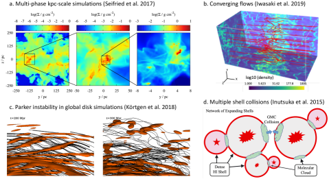
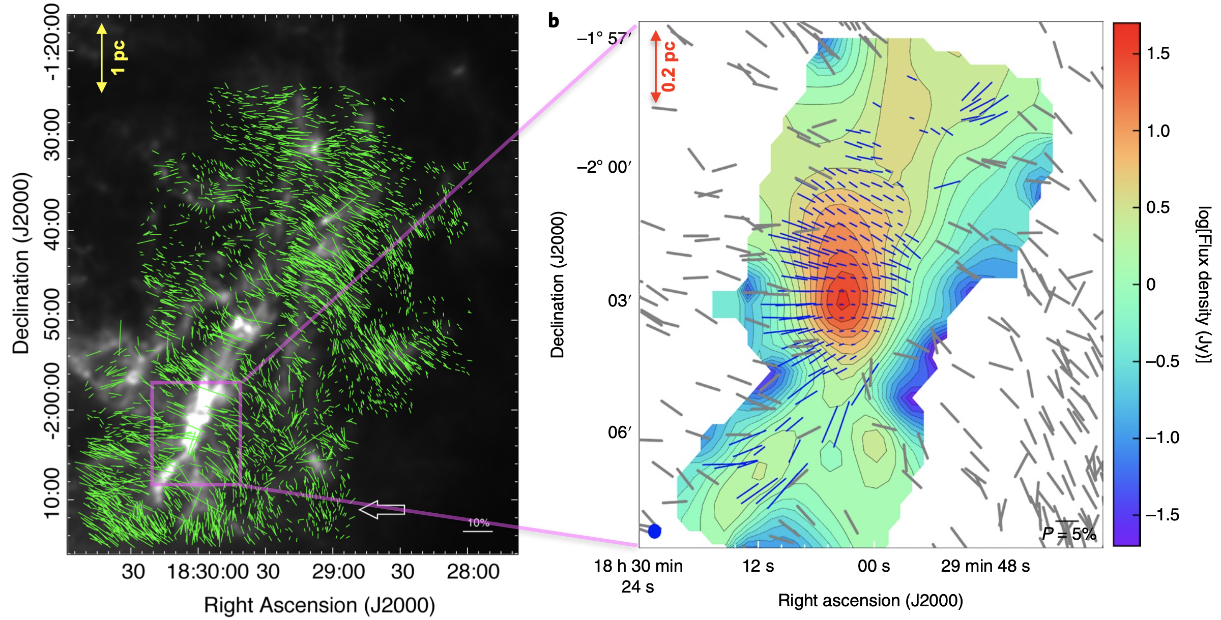
Figure 5: Cloud-formation mechanisms. (a) An example of the zoom-in technique in kpc-scaled simulations (§3.2.2) from the SILCC simulations (Seifried et al., 2017, Fig. 1; MNRAS 472 4797). Boxes show column density projections in the surroundings of a molecular cloud. (b) An illustration of colliding flows (Iwasaki et al., 2019, © AAS. Reproduced with permission) (§3.2.3), showing density in slices and the magnetic field lines along the flows and at the collision interface. (c) A close-up on diffuse clouds (brown surfaces show $10\,{\rm cm}^{-3}$ iso-density contours) formed via the Parker instability in galaxy-scale simulations, showing magnetic field lines (Körtgen et al., 2018, Fig. 3; MNRAS 479 L40) (§3.2.1). (d) An illustration of the multiple shell collision model (Inutsuka et al., 2015, reproduced with permission © ESO) (§3.2.4).

Figure 6: Left: H-band polarization vector map of the Serpens South cloud superposed on a H₂ column density map (Kusune et al., 2019, Fig. 6; PASJ 71 S5). Right: NIR polarization vector map (grey vectors; Sugitani et al. 2011) and SOFIA/HAWC+ 214 $\mu$m polarization vector map (blue vectors), superposed on the SOFIA/HAWC+ 214 $\mu m$ intensity map (Pillai et al., 2020).

3.3 Energetic importance of magnetic fields

Molecular clouds are embedded in lower-density envelopes of mostly atomic hydrogen. Zeeman H$I$1.2ex observations suggest this gas is both strongly sub-critical and has magnetic energy densities in approximate equipartition with turbulence (Heiles and Troland, 2005). Planck observations of the alignment between observed magnetic field orientation and high-latitude filamentary structures are also broadly consistent with approximate equipartition between turbulence and magnetic fields in the diffuse ISM (Planck Collaboration et al., 2016a).

Thompson et al. (2019) published 38 OH absorption Zeeman measurements, which do not target dense sub-regions and therefore trace mostly lower-density molecular gas. They find a mean LOS magnetic strength field $\langle B_{\textsc{los}}\rangle=7.4\,\pm\,0.4\,\mu G$. If the 3D field orientations of these sightlines are randomly distributed, then $\langle B\rangle\,\approx\,2\,\langle B_{\textsc{los}}\rangle$, implying the mean total field strength is $\approx 15\,\mu$G, which is larger than the $\langle B\rangle\,\approx\,6\,\mu$G derived by Heiles and Troland (2005) for H$I$1.2ex. No column density estimates, velocity line widths, or density estimates have been published yet for this sample so it is not possible to estimate the mass-to-flux ratio $\mu_{\Phi}$, or Alfvén Mach number $\mathcal{M}_{A}$.

Dust polarization observations are consistent with models where cloud-scale ($>$ 1 pc) magnetic fields are dynamically important. Planck Collaboration et al. (2016c) observations of 10 nearby clouds show a change in the preferred orientation of column density ($N_{\mathrm{H}}$) structures with respect to $\hat{B}_{\mathrm{pos}}$ from parallel to perpendicular as $N_{\mathrm{H}}$ increases (Fig. 3a), which is most consistent with simulations where the clouds are on average sub- or trans-Alfvénic. Similarly, DCF $B_{\textsc{pos}}$ estimates shown in Fig. 2 and discussed in §2.3.3 are mostly consistent with trans- or sub-Alfvénic gas motions (though as discussed in §6.1.1 these estimates tend to be systematically higher than Zeeman $B_{\textsc{los}}$ estimates at the same $n_{\textsc{H}}$). King et al. (2018) showed using Athena colliding flow simulations that the individual and joint PDFs of polarization fraction $p$ and local angle dispersion $\mathcal{S}$ are sensitive to both $\mathcal{M}_{A}$ and the mean field inclination angle $\gamma$. Applying these techniques to Planck and BLASTPol observations of 9 nearby clouds, Sullivan et al. (2021) found the $\log(p)$ vs $\log(\mathcal{S})$ slope and $\langle\mathcal{S}\rangle$ better match a slightly super-Alfvénic simulation, than a sub-Alfvénic cloud simulation. However, the authors note that if the calculation of $v_{A}$ only considers the velocity component perpendicular to the field direction (rather than the 3D velocity), the super-Alfvénic simulation would be considered trans-Alfvénic.

Line-of-sight velocity structure can also indicate the relative importance of gas turbulence and magnetic fields. Thin spectral cube channel maps, where the velocity width is much smaller than the $\sim$several km/s turbulent linewidth of a GMC, are expected to be more affected by the turbulent velocity structure of the gas than the density structure (Lazarian and Pogosyan, 2000). Heyer and Brunt (2012) used principal component analysis of thin ¹²CO and ¹³CO spectroscopic channels in the Taurus molecular cloud to measure velocity anisotropy. They found a velocity anisotropy aligned with the magnetic field towards low column density cloud sightlines, from which they inferred that the outer cloud envelope of Taurus is sub-Alfvénic, while the dense gas structures are super-Alfvénic. Lazarian et al. (2018) used synthetic observations of turbulent MHD simulations to infer $\mathcal{M}_{A}$ from the PDFs of thin velocity channel gradient orientations. Applying this method to ¹³CO observations of five molecular clouds, Hu et al. (2019) estimated mean cloud $\mathcal{M}_{A}$ ranging from 0.6 to 1.3.

Note that the observations discussed in this section show evidence of significant scatter in the estimated values for the mean Alfvén Mach number $\langle\mathcal{M}_{A}\rangle$ of individual clouds and within different sub-regions of molecular clouds (e.g.,  Hu et al., 2019; Heyer et al., 2020). They are therefore consistent with molecular clouds having near equipartition between turbulence and magnetic fields, but with localized regions of sub- and super-Alfvénic gas motions.

At higher densities ($n_{\mathrm{H}}\,\gtrsim 1000$ cm^-2), OH and CN Zeeman measurements show that the maximum $|B_{\textsc{los}}|$ magnetic field strength begins to increase rapidly with $n_{\textsc{h}}$ (Crutcher et al. 2010; Crutcher 2012; see also Fig. 2 upper left panel). The exact density of the transition from a fairly flat distribution of $|B_{\textsc{los}}|$ vs. $n_{\textsc{h}}$, to a power-law increase has been the subject of some controversy (see discussion in §6.1.2). However most authors agree that the transition is due to the onset of gravitational collapse, which under conditions of flux freezing will increase the magnetic field strength (Mestel, 1966; Li et al., 2015b; Chen et al., 2016; Ibáñez-Mejía et al., 2021).

Interestingly, the column density at which $|B_{\mathrm{LOS}}|$ begins to show a power-law increase, $\log_{10}(N_{\mathrm{H}}/$cm${}^{-2})\sim 22$, (Crutcher and Kemball, 2019) is roughly the same as the column density above which structures tend to align perpendicular to the magnetic field rather than parallel $\log_{10}(N_{\mathrm{H}}/$cm${}^{-2}){\sim 21.7}$, though the transition column density shows considerable variation from cloud to cloud and between different sub-regions (Planck Collaboration et al., 2016c; Soler et al., 2017; Soler, 2019). The number density at which $|B_{\textsc{los}}|$ increases (Crutcher et al. 2010: $n{{}_{H}}\,\sim\,300\,{\rm cm}^{-3}$) is also similar to the characteristic density where gas alignment changes from parallel to perpendicular to $\hat{B}_{\mathrm{pos}}$ in Vela C ($n_{\mathrm{H_{2}}}\,\sim 10^{3}\,$cm^-3; Fissel et al. 2019), and the density above which nearby filaments observed with Planck ($n_{\mathrm{H}}\,>\,1200\,{\rm cm}^{-3}$; Alina et al. 2019) preferentially align perpendicular to the background magnetic field. Chen et al. (2016) analysed Athena colliding flow simulations and found that both transitions roughly correspond to the density where kinetic energy due to gravitational contraction becomes larger than the magnetic energy. This interpretation agrees with Soler and Hennebelle (2017) who found that the change in relative alignment is caused by convergent gas flows, such as gravitational contraction of gas into dense filaments.

3.4 Magnetic fields and substructure formation

If a magnetic field is well coupled to the gas, and dynamically important ($\mathcal{M}_{A}\lesssim 1$), it should also influence the formation of cloud substructure. Strong magnetic fields result in anisotropic turbulence (which seeds structure formation), and set a preferential gas flow direction parallel to the field while resisting compression in the direction perpendicular to the field lines. Magnetic fields can also help shape and reinforce long filamentary structures. For example, Li and Klein (2019) show that a moderately strong magnetic field ($\mathcal{M}_{A}\sim 1$) is crucial for maintaining long and thin filamentary clouds for a long period of time, $\sim$0.5 Myr.

As discussed in the previous section, observations of molecular clouds show a clear statistical correlation between the orientation of cloud structure and the magnetic field morphology. In the last few years, more and more optical/NIR starlight polarization observations (e.g., Kusune et al., 2016; Santos et al., 2016; Kusune et al., 2019; Sugitani et al., 2019) as well as sub-mm dust continuum polarization observations (e.g., Pillai et al., 2015; Li et al., 2015a; Planck Collaboration et al., 2016b; Cox et al., 2016; Liu et al., 2018a; Alina et al., 2019; Tang et al., 2019; Fissel et al., 2019; Soam et al., 2019b; Pillai et al., 2020; Doi et al., 2020; Arzoumanian et al., 2021) have observed the magnetic fields surrounding filaments. These observations show that dense filaments preferentially align perpendicular to the direction of the local magnetic field, while lower-density filaments or striations tend to align parallel to the magnetic field.

For example, toward the nearby Musca cloud ($d\sim$ 200 pc), Cox et al. (2016) find that both the low $N_{\mathrm{H}}$ filaments or striations and $B_{\textsc{pos}}$ are oriented close to perpendicular to the high-density main filament, similar to observations of the Taurus B211/213 filament system (Chapman et al., 2011; Palmeirim et al., 2013). Cox et al. (2016) propose a scenario in which local interstellar material has condensed into a filament that is accreting background matter along field lines through the striations. Kusune et al. (2019) find that the filaments in the Serpens South cloud are roughly perpendicular to the global magnetic field (see the left panel of Fig. 6). They speculate that the filaments are formed by fragmentation of a sheet-like cloud that was created through the gravitational contraction of a magnetized, turbulent cloud.

Planck Collaboration et al. (2016c) statistically quantified this change in alignment using the histogram of relative orientations (HRO) method described in §2.3.4 on 10 nearby clouds. Fig. 3a shows that low-$N_{\mathrm{H}}$ structures tend to align parallel to the local magnetic field. The degree of alignment with the magnetic field then decreases with increasing $N_{\mathrm{H}}$, before changing to preferentially perpendicular in most clouds above $log_{10}(N_{\mathrm{H}}/{\rm cm}^{-2})\approx 21.7$. Such transitions in relative orientation only occur in simulations where cloud fields are dynamically important (e.g., Soler et al. 2013; Hull et al. 2017; lower panel of Fig. 3a), as discussed in §3.3 and §6.1.3.

Alina et al. (2019) further analysed the relative orientations between filaments, embedded clumps, and background magnetic fields for a sample of 90 Planck Galactic Cold Clumps (PGCCs) embedded in filaments where the background magnetic field orientation is uniform. They find that relative orientations between the filaments and their background magnetic field depend on the contrast in $N_{\mathrm{H}}$ between the filaments and their background environment. In low-density ($N_{\mathrm{H,bkg}}<1.2\times 10^{21}$ cm^-2) environments, low-density contrast ($\Delta N_{\mathrm{H}}<4\times 10^{20}$ cm^-2) filaments preferentially have a parallel relative alignment with the background magnetic field, however, high-contrast ($\Delta N_{\mathrm{H}}>4\times 10^{20}$ cm^-2) filaments show no preferred orientation. Interestingly, PGCC-identified filaments embedded in dense background environments ($N_{\mathrm{H,bkg}}>1.2\times 10^{21}$ cm^-2) do not show any preferential orientation relative to the background magnetic field. In addition, filaments with densities larger than $\sim$1200 cm^-3 are mostly perpendicular to the background magnetic field (Alina et al., 2019).

Using polarization data at 250, 350, and 500 $\mu$m obtained by BLASTPol, Soler et al. (2017) found that the relative orientation between gas column density structures and the magnetic field changes progressively with increasing gas column density in the filamentary Vela C giant molecular cloud (see Fig. 3c). They find that the transition of the relative orientations depends strongly on the shape of the column density probability distribution functions (PDFs). The two regions with prominent power law tails in the column density PDFs have the clearest transitions from parallel to perpendicular alignment. This could indicate that in regions where the change in orientation is prominent, the initial flows that created these regions were aligned close to the magnetic field direction, allowing dense gas to form efficiently without significantly increasing the magnetic flux.

Soler (2019) later analyzed the relative orientations of structures in 36^′′ FWHM Herschel column density maps, relative to 10^′ FWHM resolution Planck 353 GHz maps of inferred ${\hat{B}_{\textsc{pos}}}$ for the 10 nearby (d $<$ 450 pc) clouds previously studied by Planck Collaboration et al. (2016c). In contrast to Soler et al. (2017), Soler (2019) found that in cloud sub-regions with the steepest $N_{\mathrm{H}}$ power-law tail slopes (power-law index $\alpha\gtrsim 2$), which are usually interpreted to indicate a region where the energetics are mostly turbulence rather than gravity dominated, the high-$N_{\mathrm{H}}$ structures tend to be aligned perpendicular to the magnetic field. In contrast, regions with the shallowest high-$N_{\mathrm{H}}$ power-law slope, which are generally thought to be the result of gravitational collapse of high density gas, have a mean alignment angle between $N_{\mathrm{H}}$ and $B_{\textsc{pos}}$, $\langle\phi\rangle$, closer to zero, indicating preferentially parallel alignment. These results suggest that the relationship between the cloud/B-field may be more complicated than was inferred by Soler et al. (2017). Soler (2019) suggest that clouds with steep power-law slopes could represent sub-critical clouds, where strong magnetic support inhibits the formation of a high $N_{\mathrm{H}}$ power-law tail (Auddy et al., 2018). However, this steep $N_{\mathrm{H}}$ power-law tail sample includes Orion A, the most active star forming region within 500 pc distance, which is unlikely to be subcritical.

The transition in magnetic field vs. cloud structure alignment also depends on gas volume density. Fissel et al. (2019) compared the magnetic field orientation for the Vela C cloud inferred from 500 $\mu$m BLASTPol polarization maps to the orientation of elongated structures in Mopra integrated line intensity maps for nine different molecules. They find that the transition from parallel to no preferred/perpendicular alignment occurs between the densities traced by ¹³CO and by C¹⁸O, which they estimate to be $n_{{\rm H}_{2}}\sim$10³ cm^-3 (Fissel et al., 2019). This is similar to the transition density found by Alina et al. (2019) in the nearby dense filaments found in the PGCCs catalog, and to the $\hat{B}$ vs. $n$ transition density for some large scale simulations (e.g., Seifried et al. 2020).

Simulations also show that magnetic fields can influence the formation of dense filamentary structures. Inoue et al. (2018) find that the shock compression of a turbulent inhomogeneous molecular cloud creates massive filaments, which lie perpendicular to the background magnetic field. Beattie and Federrath (2020) find that for cases with a strong magnetic field, corresponding to Alfvén Mach number $\mathcal{M}_{A}<1$, and turbulent Mach number $\mathcal{M}<4$, the anisotropy in the column density is dominated by thin striations aligned with the magnetic field, while for $\mathcal{M}>4$ the anisotropy is significantly changed by high-density filaments that form perpendicular to the magnetic field. The strength of the magnetic field appears to control the degree of anisotropy, but it is the turbulent motions controlled by $\mathcal{M}>4$ that determine which kind of anisotropy dominates the morphology of a cloud.

Strong magnetic fields can also inhibit gravitational collapse by providing pressure support in the direction perpendicular to the magnetic field, which inhibits fragmentation. This is further discussed in the section on filament fragmentation (§4.2). In RAMSES simulations presented by Hennebelle (2013), hydrodynamical simulations without a magnetic field quickly fragment, while the filamentary structures that form in the MHD simulations remain more coherent, with the filaments confined by the Lorentz force. A subsequent study by Ntormousi et al. (2016) that includes non-ideal MHD turbulence including ambipolar diffusion of neutrals with respect to the ions shows that such effects make the filamentary structures broader and more massive. Note that these simulations did not include gravity.

3.5 Correlations between cloud magnetism and star formation

According to the theory of turbulent fragmentation, the distribution of stellar masses at birth (Initial Mass Function or IMF) is intimately connected to the Core Mass Function (CMF),which mirrors the overdensity distribution of supersonic turbulence (Padoan et al., 1997; Hennebelle and Chabrier, 2008, 2009). This hypothesis has led to the suggestion that isothermal, MHD turbulence might be sufficient to explain the observed peak of the IMF (Haugbølle et al., 2018), and in particular, its characteristic mass of $\sim$0.3 M_⊙. However, ideal, isothermal MHD turbulence imposes no characteristic scale, allowing filaments and cores to fragment up to the resolution limit (e.g., Federrath et al. 2017; Lee and Hennebelle 2019). On the other hand, several numerical experiments have reported little or no dependence of the shape of the IMF on magnetization (Ntormousi and Hennebelle, 2019; Guszejnov et al., 2020), even in non-ideal MHD (Wurster et al., 2019). Instead, Lee and Hennebelle (2019) showed that the dominant factor determining the shape of the IMF is the adiabatic high-density end of the equation-of-state. The magnetic field affects the peak IMF mass only when assigned unrealistically high values.

Conversely, numerical simulations show that magnetization plays a crucial role in setting the star formation efficiency (SFE) of molecular clouds (see Hennebelle and Inutsuka 2019 and Krumholz and Federrath 2019 for extensive reviews). Models of kpc-sized regions report suppression of the dense gas fraction and the overall star formation rate (SFR) of the model with increasing magnetic field strength (Iffrig and Hennebelle, 2017; Pardi et al., 2017; Girichidis et al., 2018b). Simulations of individual or colliding clouds (Wurster et al., 2019; Wu et al., 2020), massive, turbulent, star-forming clumps (Myers et al., 2014), and turbulent pc-sized GMC regions (Federrath, 2015) all show that with increasing magnetic field strength, the SFR decreases.

However, there are only a few observational studies of this connection. Li et al. (2017) investigated the correlation between magnetic field and star formation rate (SFR) in Gould Belt clouds. They argued that the clouds with a magnetic field predominantly perpendicular to their main axis consistently have lower SFR per solar mass than those with parallel alignment. However, Soler (2019) found no evident correlation between the SFRs and the magnetic field orientation in the same clouds, leaving open the question of a possible correlation between magnetization and SFR.

4 MAGNETIC FIELDS INSIDE DENSE FILAMENTS

Thermal dust emission imaging surveys with the Herschel Space Observatory have discovered ubiquitous filamentary structures in nearby Giant Molecular Clouds (GMCs) and distant Galactic Plane clouds (André et al., 2010, 2014; Schisano et al., 2020). Herschel observations also revealed that more than 70% of prestellar cores and protostars are embedded in the densest filaments, with column densities exceeding $\sim 7\times 10^{21}$ cm^-2, in nearby molecular clouds (André et al., 2014; Könyves et al., 2015), strongly suggesting that dense filaments play a very important role in star formation. Numerical simulations have also found that magnetic fields are dynamically important in the formation of filaments as well as dense cores in molecular clouds (see §3.2 and 3.4). MHD simulations (Li and Klein, 2019) performed for the formation of large-scale filamentary clouds suggest a complicated evolutionary process involving the interaction and fragmentation of dense velocity-coherent fibers into chains of cores, resembling observations in nearby clouds, such as in L1495/B213 (Hacar et al., 2013). Observations of magnetic fields inside dense filaments (M${}_{line}\geq 16~{}{\rm M}_{\odot}~{}{\rm pc}^{-1}$; André et al., 2014), where the majority of dense cores and stars form, however, were very rare a decade ago.

4.1 Magnetic field geometry inside dense filaments and filamentary clouds

As discussed in §3.4, observations indicate a trend that dense filaments preferentially align perpendicular to the direction of the local magnetic field. Magnetic fields inside dense filaments, however, are much more complicated than background magnetic fields due to interplay between magnetic fields, turbulence, gravity and stellar feedback (see Fig. 1 for example; Arzoumanian et al., 2021).

In the last few years, high-sensitivity and -resolution polarization observations with large single-dishes (e.g., JCMT, CSO, SOFIA) and interferometers (e.g., SMA, ALMA) have been resolving magnetic fields inside filaments at $<$0.1 pc (e.g., Li et al., 2015a; Pattle et al., 2017; Ching et al., 2018; Koch et al., 2018; Cortes et al., 2019; Pillai et al., 2020; Doi et al., 2020; Arzoumanian et al., 2021; Liu et al., 2020; Guerra et al., 2021; Fernández-López et al., 2021). These observations are crucial for studying the roles of magnetic fields in the formation of dense cores and stars inside filaments.

4.1.1 Nearby filamentary clouds

The JCMT B-fields In STar-forming Region Observations (BISTRO) survey has observed several filamentary clouds and revealed the magnetic field structures inside them. The first BISTRO polarization mapping of the OMC 1 region at 850 $\mu m$ found magnetic fields oriented parallel to low-density, non-self-gravitating filaments, and perpendicular to higher-density, self-gravitating filaments (Ward-Thompson et al., 2017). The densest region of the integral shaped filament in OMC 1 shows an hourglass field morphology, which is likely caused by the distortion of an initial field that is linear across the filament by the gravitational fragmentation of the filament and/or the gravitational interaction of clumps inside the filament (Pattle et al., 2017). Chuss et al. (2019) performed polarimetric observations of OMC 1 with SOFIA/HAWC+ at 53, 89, 154, and 214 $\mu m$. They find that at longer wavelengths (154 and 214 $\mu m$), the inferred magnetic field configuration matches the ‘hourglass’ configuration seen in previous observations. However, the field morphology, differs at the shorter wavelengths (53 and 89 $\mu m$), specifically close to the Orion KL region because the short wavelength data preferentially sample the warm dust that corresponds to Orion BN/KL and the associated explosion, while the long-wavelength polarimetry is likely tracing the cooler outer part of the cloud (Chuss et al., 2019; Guerra et al., 2021).

In BISTRO survey data, the polarized emission from individual filamentary structures of NGC 1333 in the Perseus GMC is spatially resolved at 0.02 pc resolution (Doi et al., 2020). The inferred magnetic field structure at 850 $\mu$m is complex, with each individual filament aligned at a different position angle relative to the local field orientation. Analysis combining the BISTRO data with low- and high- resolution data derived from Planck and interferometers (CARMA) indicates that the magnetic field morphology drastically changes below a scale of $\sim$1 pc and remains continuous from the scales of filament widths ($\sim$0.1 pc) to that of protostellar envelopes ($\sim$0.005 pc or $\sim$1000 au). Doi et al. (2020) argued that the observed variation of the relative orientation between the filament axes and the magnetic field angles is mainly caused by projection effects, and that in 3D space the B-field and the long axis of a filament are more likely perpendicular to each other.

NGC 6334, one of the nearest (d$\sim$1.3 kpc) filamentary clouds forming high-mass stars, has also been extensively studied in polarimetric observations at various scales (see Fig. 1). From optical polarimetry and high angular resolution sub-mm polarization measurements on 100–0.01 pc scales, Li et al. (2015a) found that there exist elongated gas structures nearly perpendicular to the fields at all scales. However, the fields are symmetrically pinched near density peaks in many gas elongations (filaments or cores). Using BISTRO data, Arzoumanian et al. (2021) revealed the characteristics of the small-scale ($\sim$0.1 pc) magnetic field structure of the 10 pc-long hub-filament system in NGC 6334. They found variation in the field orientation and energy balance along the crests of sub-filaments. However, at smaller scales ($\sim$1 pc), the POS magnetic field ($B_{\textsc{pos}}$) angle varies coherently along the crests of the filament network. Along the sub-filaments that surround the densest ridge or hub structures, $B_{\textsc{pos}}$ rotates from being mostly perpendicular or randomly oriented with respect to the crests to mostly parallel as the sub-filaments merge with the ridge and hubs. Arzoumanian et al. (2021) argue that this variation of the B-field structure along the sub-filaments may be caused by local velocity flows of infalling matter in the ridge and hubs.

Pillai et al. (2020) also found a transition in relative orientation along the southern filament that connects to the hub region in the Serpens South cloud (see Fig. 6, right panel), that is, a return from perpendicular to parallel alignment at A${}_{V}\sim$21 mag (see Fig. 3, panel b). They argue that this transition may be caused by gas flow, indicating that gravitational collapse and star cluster formation can occur even in the presence of relatively strong magnetic fields.

Variation of the magnetic field structures surrounding or along filaments due to gravitational collapse or gas accretion is also seen simulations. Zamora-Avilés et al. (2017) performed 3D, self-gravitating MHD simulations, finding that filaments (and subfilaments) may form by accretion/infall from the surrounding medium, driven by gravity rather than turbulence. Material accretes along the magnetic fields, which are oriented preferentially perpendicular to the filament skeleton. The magnetic field is at the same time dragged and bent by the velocity field due to the gravitational collapse. Gómez et al. (2018), simulating molecular clouds undergoing global, multi-scale gravitational collapse, also find that the magnetic field is dragged by the collapsing gas in and around filaments. Around the filament, gas is accreted onto its skeleton and the magnetic lines are perpendicular to the skeleton. However, as the gas density increases approaching the filament, the gas flow changes direction, becoming almost parallel to the filament, and field lines are dragged to align with the filament. At the spine of the filament, however, field lines become perpendicular again since they must connect to the opposite side of the filament, resulting in ‘U’-shaped magnetic structures, which tend to be stretched by the longitudinal flow along the filament. This picture is quite consistent with results from polarimetric observations of NGC 6334 (Arzoumanian et al., 2021) and Serpens South (Pillai et al., 2020).

4.1.2 Distant filamentary clouds/clumps

Magnetic fields inside distant massive filaments that may give birth to high-mass stars were barely known a decade ago due to observational difficulties: most of these clouds are located several kpc away on the Galactic Plane. Since then, high resolution and high sensitivity polarization observations of distant and massive filamentary clouds have started to tackle this problem, revealing ordered magnetic field structures within them: the overall magnetic fields inside IRDCs G11.11-0.12 (Pillai et al., 2015), G035.39-00.33 (Liu et al., 2018a), G34.43+0.24 (Tang et al., 2019; Soam et al., 2019b) and G14.225-0.506 (Añez-López et al., 2020) are perpendicular to the long axis of the main dense filaments. However, such observations are still very rare.

Pillai et al. (2015) studied magnetic fields inside two IRDCs, G11.11-0.12 and G0.253+0.016, using JCMT/SCUPOL. Magnetic fields inside G11.11-0.12 are perpendicular to the main dense filament, but are parallel to the lower density filament that merges onto the main filament. In the G0.253+0.016 cloud, close to the Galactic center, the overall magnetic field morphology as well as the cloud morphology resemble an arched structure opening to the west, which is likely caused by strong shocks in this region.

Liu et al. (2018a) observed the massive IRDC G035.39-00.33 with JCMT/POL-2 (see Fig. 7, right panel). They found that the magnetic fields tend to be perpendicular to the densest part of the main filament. The magnetic fields, however, turn to become parallel to the main filament in the two ends of the main filament. The magnetic fields also tend to be parallel to the low-density elongated structures that are connected to the main filament. The magnetic fields in the southern region of the main filament are likely pinched, hinting at an accretion flow along the filament or gravitational collapse of the massive dense cores therein. The magnetic fields in the northern region of the main filament are parallel to the filament skeleton, which is likely caused by shocks induced by a cloud-cloud collision.

Inside another massive filamentary cloud, G34.43+00.24, Soam et al. (2019b) found that the core-scale ($\sim$0.1 pc) magnetic field lines seen with large single-dishes (JCMT/POL-2 and CSO) appear to be connected to the small-scale ($\sim$0.01 pc) field geometry traced by interferometers (CARMA, SMA) and large-scale ($\sim$10 pc) field lines traced by Planck. In the same cloud, Tang et al. (2019) found a close alignment between local magnetic field orientations and local velocity gradients (see Fig. 7, left panel). This local correlation in alignment suggests that gas motions are influenced by the magnetic field morphology, or vice versa.

Wang et al. (2020b) observed a filament-hub system G33.92+0.11. In the high-density areas, their analysis shows that the filaments tend to align with the magnetic field and local gravity. In the low-density areas, they find that the local velocity gradients tend to be perpendicular to both the magnetic field and local gravity, although the filaments still tend to align with local gravity.

However, none of these single-dish observations resolved magnetic fields down to 0.1 pc scale, preventing comparative studies between these distant clouds and nearby clouds. ALMA will have adequate sensitivity/resolution to resolve magnetic fields down to $<0.1$ pc for these distant clouds in dust polarization or Zeeman observations with its mosaic mode.

4.2 The role of magnetic fields in filament stability and fragmentation

André et al. (2014) proposed a paradigm for star formation in which filaments play a fundamental role, based on Herschel Gould Belt survey results. They argued that prestellar cores are formed through gravitational fragmentation of the densest filaments above the thermally critical mass per unit length, $M_{line,crit}\approx 16M_{\odot}\,{\rm pc}^{-1}$ (for a molecular gas temperature of $\sim$10 K). André et al. (2019b) further demonstrated that the filament mass function (FMF) and the filament line mass function (FLMF) show very similar shapes that are both consistent with a Salpeter-like power-law function, suggesting that the stellar initial mass function (IMF) may originate from gravitational fragmentation of individual filaments.

The magnetic field, which is not much discussed in this paradigm (André et al., 2014; André et al., 2019b), could also play an important role in stabilizing filaments and regular filament fragmentation, as well as star formation inside filaments (Nagasawa, 1987). Fiege and Pudritz (2000) found that a poloidal field inside a filament helps to support the filament radially against self-gravity, increasing $M_{line,crit}$, while a toroidal field works with gravity in squeezing the filament, reducing $M_{line,crit}$. Tomisaka (2014) calculated magnetohydrostatic configurations of isothermal filaments that are laterally threaded by a magnetic field, finding that the magnetic field supports the filament by increasing the maximum line-mass supported against self-gravity, and that the maximum mass of the magnetized filament is significantly affected by the magnetic field when the magnetic flux per unit length ($\Phi_{\rm cl}$) exceeds $\Phi_{\rm cl}\gtrsim 3\,{\rm pc\,\mu G}\,(c_{s}/190\,{\rm m\,s^{-1}})^{2}$.

Seifried and Walch (2015) performed a set of 3D MHD simulations of magnetized filaments with various $M_{line}$ values and magnetic field orientations with respect to the major axis. They found that magnetic fields perpendicular to the major axis cannot contribute to the stabilization of supercritical filaments, resulting in filament widths $<0.1$ pc. Conversely, a magnetic field parallel to the major axis can stabilize the filament against radial collapse, resulting in widths of 0.1 pc, in agreement with the observed filament width found in nearby clouds (André et al., 2010, 2014). Seifried and Walch (2015) also discovered three filament collapse modes: edge-on, uniform, and centralized, depending on M_line. They found that filaments with M_line equal to $M_{line,crit}$ (M${}_{line,crit}\sim 25~{}{\rm M}_{\odot}~{}{\rm pc}^{-1}$ for gas at 15 K) follow an edge-on collapse mode, with star formation taking place at the outer edges of the filaments. No or only a little fragmentation is found along the major axes of these filaments. More and more fragmentation takes place along the entire filament (uniform collapse mode) for higher M_line. The filament collapses towards its common gravitational centre (centralized collapse mode) if there is a initial moderate density enhancement in its centre (a factor of 3).

Observations of some massive filaments indicate that magnetic fields are strong (ranging from several tens of $\mu G$ to several mG), and magnetic support is comparable to kinetic (thermal and turbulent) support in stabilizing filaments (Pillai et al., 2015; Pattle et al., 2017; Liu et al., 2018a; Tang et al., 2019; Soam et al., 2019b; Arzoumanian et al., 2021).

Pattle et al. (2017) derived a very high magnetic field strength ($B_{\textsc{pos}}=6.6\pm 4.7$ mG) in the OMC 1 region. The magnetic energy density in OMC 1 is comparable to the gravitational potential energy density, suggesting that the OMC 1 region is on large scales near magnetic criticality or slightly subcritical, with $\mu_{\phi,obs}\sim 0.41$. However, Hwang et al. (2021) recently found the OMC 1 region to be supercritical, with a median value of $\mu_{\phi,obs}\sim 1.5$. This inconsistency is due to differing measurements of column density in the two works. In NGC 6334, Arzoumanian et al. (2021) find that in the outer parts of sub-filaments magnetic tension alone is not enough to balance gravity, while the inner parts of the sub-filaments seem to be in a magnetic critical balance. However, the combined magnetic and kinetic (thermal and turbulent) energies can provide sufficient support against gravity in these sub-filaments as well as in the densest ridge regions.

Pillai et al. (2015) find that the magnetic field in two distant IRDCs, G11.11-0.12 and G0.253+0.016, is strong enough to resist gravitational collapse and suppress fragmentation sufficiently to allow high-mass star formation. The $\mathcal{M}_{A}$ values in the two clouds are low, $\mathcal{M}_{A}\leq 1.2$, and the most likely values of $\mu_{\Phi,obs}$ are $<1$. Similarly, the three ridge regions (MM1, MM2, MM3) of the massive filamentary IRDC G34.43+00.24 also seem to be magnetically critical or slightly subcritical, with $\mu_{\Phi,obs}\sim 0.5-1.1$ (Tang et al., 2019). Liu et al. (2018a) find that the main filament in IRDC G035.39-00.33, a cloud at a much younger evolutionary stage than G11.11-0.12 and G34.43+00.24, has a relatively weak magnetic field ($\sim 50~{}\mu$G) and is likely unstable even if magnetic field support is taken into account.

Observational studies of fragmentation versus magnetic fields at all scales in filamentary clouds, however, are still very scarce. Toward IRDC G34.43+0.24, Tang et al. (2019) propose that the different fragmentation types seen at sub-parsec scale are determined by the varying relative importance of magnetic fields, gravity, and turbulence. In regions where magnetic field dominates over turbulence, there is aligned fragmentation (MM2) or no fragmentation (MM1), while in MM3 where the magnetic field is not dominant over turbulence, clustered fragmentation is seen (Tang et al., 2019). Añez-López et al. (2020) observed two hubs (Hub-N and Hub-S) in the IRDC G14.225-0.506 at 350 $\mu m$ using the Caltech Submillimeter Observatory (CSO). They argued that different levels of fragmentation in these two hubs could be caused by magnetic field properties rather than gas density, because the density in the two hubs is similar.

Over the last few years, more and more high sensitivity and high angular resolution interferometric observations have also been performed to study the role of magnetic fields in the fragmentation process of distant massive filaments/clumps. With ALMA, Dall’Olio et al. (2019) observed the magnetic field in the filamentary high-mass star forming clump G9.62+0.19, and found that the magnetic field is oriented along the massive filament. The high magnetic field strength and smooth polarized emission in G9.62+0.19 indicate that the magnetic field could play an important role in the fragmentation of massive filaments and that the formation and evolution of dense cores can be magnetically regulated. ALMA dust polarization observations of the W43 high-mass star forming regions hint that a strong magnetic field may suppress fragmentation of clumps/filaments (Cortes et al., 2019), and also control the angular momentum distribution from the core scale down to the inner part of the circumstellar disk where outflows are launched (Arce-Tord et al., 2020). Palau et al. (2021) studied fragmentation and magnetic field within 18 massive dense clumps using the polarization data obtained in the SMA Legacy Survey of Zhang et al. (2014). Their entire sample of massive dense clumps presents a strong correlation of the fragmentation level with the density of the parental clump. They also find a tentative trend of the fragmentation level with the mass-to-flux ratio.

Observationally, it is still hard to reach a firm conclusion on the role of magnetic fields in regulating filament fragmentation. However, more high resolution dust polarization observations with state-of-the-art single-dishes (e.g., JCMT/POL-2, SOFIA/HAWC+) or interferometers (e.g., ALMA) will allow deeper studies of magnetic fields inside large samples of filaments in the near future.

Figure 7: Magnetic field vs. velocity field for two infrared dark clouds. Left: IRDC G34.43+00.24 (Tang et al., 2019, © AAS. Reproduced with permission). Image shows gas velocity of N₂H⁺ (1-0) line emission; contours show the integrated intensity map of N₂H⁺ (1-0) line emission; white segments show magnetic field orientations inferred from polarized 350 $\mu m$ dust emission obtained with CSO. Right: IRDC G035.39-00.33 (Liu et al., 2018a, © AAS. Reproduced with permission). The image shows gas velocity of NH₃ (1,1) line emission. The black segments show magnetic field orientations inferred from polarized 850 $\mu m$ dust continuum emission obtained with JCMT/POL-2.

5 MAGNETIC FIELDS IN DENSE CORES

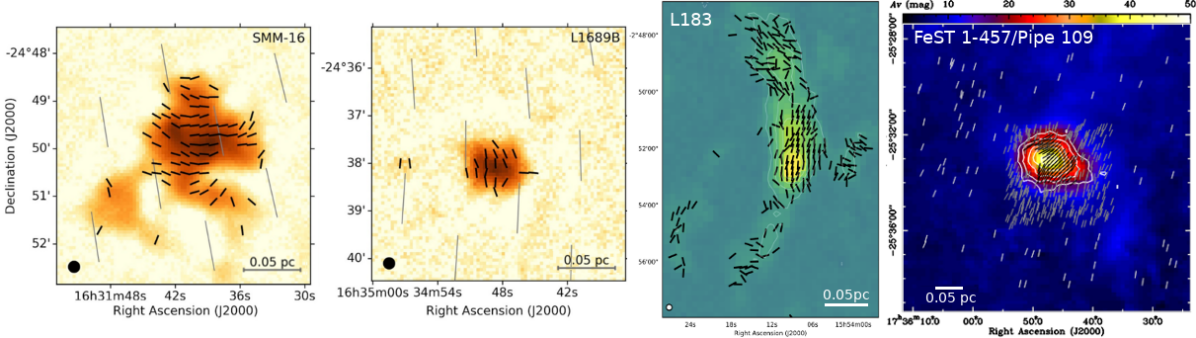
Figure 8: Recent observations of resolved magnetic fields in nearby low-mass prestellar cores. L-R: L1689 SMM-16 and L1689B (Pattle et al., 2021a, © AAS. Reproduced with permission), L183 (Karoly et al., 2020, © AAS. Reproduced with permission), FeST 1-457/Pipe 109 (Alves et al., 2014, reproduced with permission © ESO). All POL-2 observations (plus Planck large-scale field for L1689) except FeST 1-457 (PolKa, large-scale field from extinction polarimetry).

In this section we discuss magnetic fields within dense molecular cores. We consider starless cores, which, if gravitationally bound (‘prestellar’), will go on to form an individual stellar system (Benson and Myers, 1989; Ward-Thompson et al., 1994) and low-mass protostellar cores, which have formed a central hydrostatic object, in § 5.1; their high-mass counterparts (Tan et al., 2014; Motte et al., 2018) in §5.2; and the coupling of protostellar outflows to their surroundings in §5.3. We consider protostellar sources in their envelope-dominated main (Class 0) and late (Class I) accretion phases, rather than their later pre-main-sequence (Class II, III) phases (Lada, 1987; Andre et al., 1993). For a discussion of protostellar discs and outflows, see the chapter by Tsukamoto et al.

Extinction polarization traces the peripheries of dense cores (e.g., Kandori et al., 2017b) while high surface-brightness cores are detectable in emission polarization (e.g., Ward-Thompson et al., 2000), although the $A_{V}$ to which grains remain aligned remains under debate (e.g., Alves et al., 2014; Jones et al., 2015; Pattle et al., 2019), and depends on grain properties and incident radiation fields (Hoang et al., 2021). Starless cores typically lack internal structure and so are often resolved out by interferometers (e.g., Kirk et al. 2017). Protostellar cores are typically easier to observe, being brighter and more centrally condensed, with an embedded source driving grain alignment, and with internal structure (e.g., Sadavoy et al., 2018). However, interpretation can be complicated by the variety of grain alignment mechanisms around protostars (see § 2.2.3). Astrochemical analysis is therefore a key tool for investigating the dynamic importance of magnetic fields in dense cores.

5.1 Magnetic fields in low-mass cores

5.1.1 Magnetic field geometry

The classic dense core magnetic field model is an ‘hourglass’ morphology centred on the centre of mass, formed by material first collapsing freely along field lines, and the largely flux-frozen field then being dragged in by further collapse (Mestel, 1966); Ewertowski and Basu (2013) and Myers et al. (2018) present analytical 3D hourglass models. The importance of ambipolar diffusion, and so the initial $\mu_{\Phi}$ value, may be inferred from the field morphology: stronger ambipolar diffusion leads to weaker flux-freezing, and so less field curvature (Basu et al., 2009).

Submillimeter observations of starless cores show ordered, linear fields (Alves et al., 2014; Liu et al., 2019; Karoly et al., 2020; Pattle et al., 2021a), without clear hourglass morphologies, as shown in Fig. 8. Magnetic fields are typically consistent with being parallel to the core minor axis in 3D (Basu, 2000), suggesting that cores preferentially collapse along the magnetic field direction. Simulations similarly produce triaxial cores, with the magnetic field preferentially most parallel to the core minor axis and most perpendicular to the major axis (Chen and Ostriker, 2018).

Parabolic models can be fitted to NIR observations of fields in starless core peripheries; SIRPOL observations of FeST 1-457 have been extensively modeled (Kandori et al., 2017b, a, 2018a, 2018b, 2018c, 2020a), as have B335, B68, BHR 71, CrA-E and L1174 (Kandori et al., 2020b, c, d, e, f). The parabolae fitted are in some cases significantly offset from the density peak; e.g., Kandori et al. (2020f). Bino and Basu (2021) fitted SIRPOL observations of FeST 1-457’s periphery with an hourglass model, finding that the core is mildly supercritical, and may have undergone a sub-to-supercritical transition through ambipolar diffusion. However, as discussed in §5.1.5 and shown in Fig. 8, magnetic fields in the centres of starless cores can be significantly offset from the preferred axis of the field in their surroundings, including in FeST 1-457 (cf. Kandori et al., 2020a).

Recently, Sahu et al. (2021) detected extremely high density ($n>10^{7}$ cm^-3) substructures inside five evolved prestellar cores in the Orion GMC with ALMA, with a spatial resolution of $\sim$320 au. Future high-resolution dust polarization observations toward these cores will shed light on how magnetic fields behave in the central regions of prestellar cores that are developing substructure and close to the onset of protostar formation.

At least some protostellar cores have hourglass fields when viewed using interferometers (e.g. Girart et al., 2006; Maury et al., 2018), including protobinary cores (Kwon et al., 2019). MHD collapse models can give a measure of initial $\mu_{\Phi}$ and field strength, and of collapse timescale, in these cores (e.g. Frau et al., 2011). However, ALMA has shown that many protostellar sources have more complex small-scale magnetic field geometries (e.g., Hull et al., 2017), including potential magnetized accretion structures in multiple systems (e.g., Sadavoy et al., 2018). Interpretation of these observations may be complicated by polarized emission preferentially tracing outflow cavity walls (Hull et al., 2020a). How common hourglasses are in protostellar cores remains uncertain.

5.1.2 Magnetic field strength and energy balance

DCF measurements of magnetic field strength in starless/prestellar cores range from $\sim 10^{1}$ $\mu$G (e.g., Kirk et al., 2006) to a few $\times 10^{2}$ $\mu$G (e.g., Karoly et al., 2020; Pattle et al., 2021a), (cf. Fig. 2). As discussed in §6.1.1, isolated cores appear to have relatively low magnetic field strengths for their density; however, like other structures considered, their turbulence is typically found to be sub- or trans-Alfvénic. DCF-derived mass-to-flux ratios in prestellar cores range from mildly supercritical (e.g., $\mu_{\Phi}\sim 2-3$; Kirk et al. 2006) to somewhat subcritical (e.g., $\mu_{\Phi}\sim 0.1-0.4$; Karoly et al. 2020). A meta-analysis of DCF measurements of 17 nearby low-mass pre- and protostellar cores (Myers and Basu, 2021) suggests that these cores are nearly critical, with $B_{\textsc{pos}}\propto N^{1.05\pm 0.08}$ and $\propto n^{0.66\pm 0.05}$, and masses $\sim 0.5-2\times$ their virial mass. They suggest that the cores’ centrally-condensed and spheroidal geometries create the observed $\kappa\approx 2/3$, despite the cores’ magnetic fields being as strong as possible while remaining subdominant. However, Ching et al. (2022) present Zeeman measurements of the isolated prestellar core L1544, finding that both the core and its surrounding envelope are supercritical, suggesting that in at least some cases, prestellar cores may be supercritical from an early stage in their evolution.

Astrochemical analysis is a powerful tool for determining the magnetic criticality of cores. The best tracers to use remain under investigation through chemical post-processing of non-ideal MHD simulations (e.g., Ferrada-Chamorro et al., 2021). Priestley et al. (2019) suggest that HCN and CH₃OH line intensity profiles show promise as tracers of sub/super-critical collapse. Yin et al. (2021) find the peak intensity ratio of N₂H⁺ to CS lines, and the CS blue-to-red peak intensity ratio, to be useful diagnostics of the initial mass-to-flux ratio of cores. The authors apply this analysis to the core L1498, identified as supercritical by Kirk et al. (2006), and suggest that it has evolved to supercriticality from a magnetically subcritical initial state.

Spatially-resolved mapping can provide information on core evolution; ambipolar-diffusion models predict an extended region of significant depletion of many species in the inner regions of cores (Tassis et al., 2012), largely inconsistent with observations (Priestley et al., 2018). With assumptions, it may also be possible to use gas velocities to infer magnetic field strength in cores (Auddy et al., 2019).

5.1.3 Prestellar core lifetimes

Core lifetime is a key measure of the dynamic importance of prestellar core magnetic fields. A core in a state of unimpeded infall will collapse on its freefall timescale (eq. 9), while a core evolving quasistatically will have a lifetime set by the ambipolar diffusion timescale (eq. 10). For typical core conditions, $t_{AD}$ is several times larger than $t_{ff}$, although the strong-field collapse time varies between models (e.g., $\gtrsim 5-10\times t_{ff}$; Machida et al. 2018), and for sufficiently low values of $x_{e}$, $t_{AD}$ could become comparable to the freefall time, as discussed in §5.1.4.

Astrochemical studies have produced a range of results in different cores, often suggesting that chemistry in starless cores is not steady-state and that core lifetimes are $<t_{AD}$; e.g., Pagani et al. (2013), using N₂D⁺/N₂H⁺ as a chemical clock, ruled out slow contraction in L183, suggesting a core lifetime $\leq 0.7$ Myr, while Maret et al. (2013) modeled C¹⁸O and HCO⁺ in the cores L1498 and L1517B, finding ages of a few $\times 10^{5}$ yr. Recently, Bovino et al. (2021) studied the ortho-H₂D⁺/para-D₂H⁺ ratio in six cores in the Ophiuchus molecular cloud, finding core ages up to 200 kyr, consistent with $\sim 1-5\times t_{\rm ff}$, and inconsistent with $t_{AD}$. However, at least some cores appear to be longer-lived: Lin et al. (2020) found that the starless core L1512 is old enough for N₂ chemistry to be steady-state, hence $>1.4$ Myr, suggesting a lifetime $\gg t_{ff}$. These estimates can be affected by pre-processing of core material: Brünken et al. (2014) estimated the age of the IRAS 16293-2422 core as $>$1 Myr, while a reanalysis by Harju et al. (2017) found an age of $\sim 0.5\pm 0.2$  Myr, with $\sim 0.5$ Myr pre-processing.

Average core lifetimes can be estimated from number counts relative to Class II protostars (lifetime $\sim 2\,$Myr; Beichman et al. 1986), assuming that all cores considered will go on to form stars, and that the local SFR has remained constant over at least the Class II lifetime. Enoch et al. (2008), from $Spitzer$ observations of nearby clouds, found an average lifetime of $\sim 500^{+500}_{-250}$ kyr for cores with $n>2\times 10^{4}$ cm^-3, indicating dynamic rather than quasistatic evolution, while Kirk et al. (2005) found a mean lifetime $\sim 300$ kyr for SCUBA-identified prestellar cores. For a large sample of cores, lifetimes can be estimated as a function of density, and are typically $\sim 1-10\times t_{ff}$, decreasing with increasing density, suggesting that cores evolve from magnetically sub-critical at low densities to super-critical at high densities (Jessop and Ward-Thompson, 2000; Könyves et al., 2015). However, lower-density cores are less likely to be gravitationally bound, and so could be over-counted, inflating their lifetimes (Könyves et al., 2015). Das et al. (2021) presented a partial flux-freezing model which produces lifetimes similar to the Könyves et al. (2015) results, and suggest that cores are formed with a transcritical $\mu_{\Phi}$.

These results suggest that nearby, low-mass cores are generally evolving faster than the ambipolar diffusion timescale, but probably are not in freefall collapse. Lifetimes are typically a few hundred kyr, with exceptions. The lifetimes of cores forming high-mass stars, and of low-mass cores in clustered environments, remain uncertain.

5.1.4 Ionization fraction in dense cores

For ion-neutral coupling to persist in dense cores and for magnetic fields to provide any support against collapse, the ionization fraction $x_{e}$ must be sufficiently high that $t_{AD}>t_{ff}$ (e.g., Caselli et al., 1998); cloud-scale simulations show that $\mu_{\Phi}$ in dense cores increases with decreasing $x_{e}$ (Chen and Ostriker, 2014). In starless cores, $x_{e}$ is maintained by cosmic ray ionization; $t_{AD}<t_{ff}$ when $n_{H}\gtrsim 2.56\times 10^{-12}x_{e}^{-2}\,{\rm cm}^{-3}$ (Caselli et al., 1998). Caselli et al. (1998), surveying 24 dense clouds, found $x_{e}\sim 10^{-6}-10^{-8}$, with cosmic ray ionization rate $\zeta\sim 10^{-16}-10^{-18}$ s^-1, and that $t_{AD}\sim 50\times t_{ff}$ on average, although in 20% their cores, $t_{AD}$ was only a few times greater than $t_{ff}$. The highly centrally-condensed prestellar core L1544 is particularly well-studied: Caselli et al. (2002) found $x_{e}\sim 10^{-9}$, and so $t_{AD}\sim t_{ff}$. Keto and Caselli (2010) find $\zeta\sim 10^{-17}$ s^-1 in L1544, while Ivlev et al. (2019) find L1544 is consistent with $\zeta\sim 10^{-16}$ s^-1, and Bovino et al. (2020) measure 2–3$\times 10^{-17}$ s^-1.

Despite this, gas in molecular clouds may maintain a relatively high $\zeta$. In the diffuse ISM, $\zeta\sim 10^{-16}$ s^-1, decreasing with increasing $N$ (Indriolo and McCall, 2012). Fiducial values of cosmic ray ionization rate in dense gas are a few $\times 10^{-17}$ s^-1 (Caselli et al., 1998; van der Tak and van Dishoeck, 2000). However, values measured in molecular clouds can be considerably higher (e.g., $\sim 10^{-14}$ s^-1 in OMC-2 FIR4; Favre et al. 2018). Shocks associated with protostars may produce cosmic rays within molecular clouds (Padovani et al., 2016), and so $\zeta$ and $x_{e}$, and therefore $t_{AD}$ and the ion-neutral coupling in dense cores, may vary considerably both within and between clouds.

5.1.5 Relationship between core- and cloud-scale fields

Chen et al. (2020) found the statistical orientation of cores with respect to the magnetic field of their parent cloud to vary: in the Perseus molecular cloud, the angles between core axes and background magnetic field are random, while in Taurus, cores are typically perpendicular to the background field, and in Ophiuchus, under large-scale feedback, cores are typically slightly parallel to the background field.

As shown in Fig. 8, significant discrepancies can exist between magnetic field directions in dense cores, and those in their immediate surroundings. Comparisons of Planck and JCMT observations in nearby regions (Doi et al., 2020; Pattle et al., 2021a; Karoly et al., 2020), and APEX and NIR observations of FeST 1-457 (Alves et al., 2014), show that in some cores the large- and small-scale fields agree, while in others the two are perpendicular. Bok globules also in some cases show discrepancies between their internal and external fields (Das et al., 2016; Choudhury et al., 2019). Magnetic fields in cores embedded in filaments are often consistent with being perpendicular to the filament major axis, and so may be inherited from the parent filament (e.g., Pattle et al., 2021a), although there are exceptions (Eswaraiah et al., 2021), and these observations beg the question of whether the field being traced is truly that of the core, or of the filament. Simulations of ensembles of cores (Chen and Ostriker, 2018) suggest that internal and external magnetic field directions are typically correlated. The number of cores with resolved magnetic field observations remains small, and it is not yet clear whether significant discrepancies between large- and small-scale core fields are unusual.

5.2 Magnetic fields in high-mass star-forming cores

Models of high-mass star formation fall into two categories: quasistatic core accretion, in which massive stars form analogously to low-mass stars, through monolithic collapse of a virialised high-mass prestellar core (HMPSC) McKee and Tan (2003); or competitive accretion, in which stars forming in a cluster acquire mass through either accretion of a common reservoir (Bonnell and Bate, 2006), or accretion streams associated with hierarchical cloud collapse (e.g., Smith et al., 2009; Vázquez-Semadeni et al., 2017). At least some high-mass protostellar cores (Girart et al., 2009) and massive cluster-forming and fragmenting cores (Qiu et al., 2014; Beltrán et al., 2019) show hourglass magnetic field morphologies, suggestive of ordered collapse.

Massive Dense Cores (MDCs; Motte et al., 2007, 2018) are a recent observational paradigm of high-mass star formation with no HMPSC phase (Tigé et al., 2017). MDCs form within hub-filament systems, and have a starless phase, in which the MDC can contain numerous low-mass prestellar cores, followed by a star-forming phase, in which numerous low-mass protostars form, some of which become high-mass through competitive accretion from the MDC. MDCs appear to be collapsing on timescales $>t_{ff}$, with infall speeds $\sim 3-30$% of their freefall velocities (Wyrowski et al., 2016), indicating a potential role for magnetic fields in stabilising and mediating their collapse.

ALMA has observed a number of clumps and MDCs fragmenting into low-mass cores (e.g., Sanhueza et al., 2017; Louvet et al., 2019), and some fragmenting into cores with a wider range of masses (Redaelli et al., 2021). Beuther et al. (2018) and Sanhueza et al. (2019) identify samples of low-to-intermediate-mass cores in massive clumps. Beuther et al. (2018) find their cores to be near-virial and sub-Alfvénic based on DCF analysis, while Sanhueza et al. (2019) find that 19% of their 210 cores have masses $>M_{J}$.

If there is an HMPSC star formation pathway, these HMPSCs will have masses $\gg M_{J}$, and so are expected to require significant magnetic support (e.g., Tan et al., 2014). There is a short list of current HMPSC candidates (broadly defined as sources $\gtrsim 30\,$M_⊙, without internal structures and near virial equilibrium; e.g., Tan et al. 2014), G11.92-0.61-MM2 (Cyganowski et al., 2014), a $\gtrsim 30\,$M_⊙ source with no signs of star formation; the $\sim\,60$ M_⊙ core W43-MM1#6 (alternatively, a starless MDC; Nony et al., 2018); and AG354-2 (Redaelli et al., 2021). Some intermediate-mass starless cores have also been identified, e.g. G331.372-00.116 ALMA1 (Contreras et al., 2018), a $\sim$17 M_⊙ infalling PSC candidate requiring a mG field for stability.

Observations of resolved magnetic fields in high-mass star-forming clumps suggest magnetic supercriticality: Pillai et al. (2016), observing the massive star-forming clump G35.20w in W48, using SCUPOL and CN Zeeman data, found a highly ordered sub-Alfvénic magnetic field, but $\mu_{\Phi}\sim 1.5$. Liu et al. (2020) observed three MDCs in the IRDC G28.34 with ALMA, finding the cores to be sub-virial, with magnetic fields well-aligned with local gravity, suggesting gravitational collapse. However, a bimodal distribution of magnetic field/outflow axes suggests that magnetic fields could be dynamically important later in the collapse process. Recent ALMA observations of the high-mass star-forming regions G327.3 (Beuther et al., 2020) and IRAS 18089-1732 (Sanhueza et al., 2021) have found toroidal magnetic field geometries, as shown in Fig. 9, suggesting dynamics dominated by gravity and rotation, while Sanhueza et al. (2019) find $\mu_{\Phi}>8$ in IRAS 18089-1732, indicating a highly gravitationally-dominated system.

Models of turbulent massive cores suggest that magnetic fields affect fragmentation and multiplicity. Commerçon et al. (2011) find that magnetic fields suppress fragmentation, suggesting that highly magnetised MDCs could produce isolated massive stars, while moderately magnetised MDCs form small clusters. Stronger fields may also reduce fragmentation in discs around massive protostars (e.g., Peters et al., 2011; Mignon-Risse et al., 2021). Palau et al. (2021), using SMA data, find a tentative correlation between the number of embedded sources and $\mu_{\Phi}$ in a sample of MDCs, in agreement with models.

How the magnetic field geometry of a dense core changes under external feedback may be important to core evolution in massive star-forming regions. There is limited evidence that linear fields are maintained in some cores under feedback (Cortes et al., 2021b; Pattle et al., 2021b; Könyves et al., 2021), but more observations are needed.

Figure 9: ALMA 2.1mm observations of magnetic fields in the high-mass star-forming region IRAS 18089-1732 (Sanhueza et al., 2021, © AAS. Reproduced with permission). The toroidal magnetic field geometry is suggestive of dynamics dominated by gravitational collapse and rotation.

5.3 Outflows and the effects of feedback

Interferometric studies of core-scale magnetic field and outflow orientation have suggested that alignment is typically random, with a possible highly-correlated subset (Hull et al., 2014; Zhang et al., 2014; Hull and Zhang, 2019), while observations of protostellar envelopes find fields to be preferentially either parallel or perpendicular to the outflow, with misalignment more common in sources with larger rotational energies (Galametz et al., 2018, 2020). A comparable single-dish study found that outflows and local magnetic fields tend to be misaligned by $50^{\circ}\pm 15^{\circ}$ in 3D, but did not rule out random orientation (Yen et al., 2021). Alignment between protostellar outflows and larger-scale magnetic field or gas density structures may vary significantly between clouds. In G28.37+0.07, Kong et al. (2019) found protostellar outflows to be preferentially perpendicular to the IRDC, suggesting a quite strong magnetic field. Conversely, in Perseus, Stephens et al. (2017) found outflow-filament angles consistent with either random alignment or a mix of projected parallel and perpendicular angles.

The initial magnetic field strength of a collapsing core may significantly affect its protostellar outflows: in strong-field collapse, the angular momentum of the star-forming cloud may be efficiently transferred away before rapid collapse begins, resulting in weaker outflows (Machida et al., 2018). Magnetic fields couple such outflows to the surrounding cloud; these outflows provide feedback on very short timescales ($\lesssim 10^{4}$ yr), switching on as soon as either a low- and high-mass protostar forms (e.g., Krumholz and Federrath, 2019). We discuss this in §6.3.

6 SYNTHESIS

We now return to the questions posed in §1 and the methods described in §2 to discuss our current understanding of how magnetic fields affect the star formation process across the range of size and density scales considered in §3–5.

6.1 Energy balance

6.1.1 The reliability of DCF analysis

We here discuss the DCF measurement compilation presented in § 2.3.3 and Fig. 2. Fig. 2b shows little systematic difference between DCF variants. We do not have space in this chapter to perform a fair and thorough comparison of the various DCF methods, and so we refer the reader to Liu et al. (2021a); Liu et al. (2021b) for detailed discussion of this point.

Fig. 2c shows continuity between extinction and emission measurements. Extinction measurements do not trace high $A_{V}$, while emission measurements lack the pencil-beam resolution of extinction measurements, and so this continuity suggests similar magnetic field dispersion across a wide range of scales. The high-density breakdown in the correlation between $B_{\textsc{pos}}$ and $n$ is exclusive to the interferometric points. This could perhaps be due to instrumental effects (e.g., spatial filtering), or to DCF failing on small scales (Liu et al., 2021a). It is unlikely to be caused by $\sigma_{v,\textsc{nt}}$ tracing infall motions, as the $B_{\textsc{pos}}$ values decrease rather than increase, and this behavior appears to result from an increase in $\mathcal{M}_{A}$, which is independent of $\sigma_{v,\textsc{nt}}$. The apparent decreases in $B_{\textsc{pos}}$ are predominantly seen in distant ($>$ 1 kpc) star-forming clumps. Nearby protostellar sources and HH objects have $\mathcal{M}_{A}\sim 1$ to the highest densities.

Fig. 2d qualitatively suggests that isolated cores have lower $B_{\textsc{pos}}$ for a given $n_{\textsc{h}}$ than do structures under feedback. However, there is no distinction in their $\mathcal{M}_{A}$ values (Fig. 2f); the differences appear to arise from the isolated sources having smaller $\sigma_{v,\textsc{nt}}$, and so lower $v_{A}$, (Fig. 2e). ‘Cloud structures’ is a broad category and covers a wide range of $B_{\textsc{pos}}$ values. Protostars, jets, and HH objects have quite high $B_{\textsc{pos}}$ values, although these measurements are mostly at high densities where DCF is most uncertain. Interestingly, the few extragalactic measurements appear to be broadly similar to those made within the Milky Way.

We measured the mean DCF- and Zeeman-derived magnetic field strength over each decade in density, and found that the $\langle B_{{\rm DCF}}\rangle/\langle B_{{\rm Zeeman}}\rangle$ ratio varies in the range 1–18, with an average of $B_{{\rm DCF}}/B_{{\rm Zeeman}}=6.3\pm 1.5$, where the uncertainty is standard error on the mean (the median ratios produce a similar value). It is important to note that these compilations are not well-controlled or homogeneous samples, and that the DCF and Zeeman measurements may not have been made in the same environment at a given density. Moreover, measurements of gas density from paramagnetic species and from dust emission will themselves be subject to differing systematic uncertainties. However, this ratio is similar to previous results: Poidevin et al. (2013), comparing CN and OH Zeeman to SCUPOL DCF measurements of matched regions, found $B_{{\rm DCF}}/B_{\rm Zeeman}=4.7\pm 2.8$, while Soler et al. (2018), comparing HI Zeeman to $Planck$ DCF measurements of the Eridanus superbubble, found $B_{\rm DCF}/B_{\rm Zeeman}\sim 2.5-13$.

However, Zeeman measurements trace $B_{\textsc{los}}$ while DCF traces $B_{\textsc{pos}}$, and $\langle B_{\textsc{pos}}\rangle/\langle B_{\textsc{los}}\rangle$ $=(\pi/4)/(1/2)$ $=1.58$ (cf. Pillai et al. 2016). This suggests that if the Zeeman measurements are treated as an accurate reference for $B_{\textsc{los}}$ (cf. § 2.2.1), then the DCF measurements in Fig. 2 on average overestimate $B_{\textsc{pos}}$ by a factor $\sim 3-5$. We note however that there is significant uncertainty on this value, and further that this is, if valid, a statistical correction to the ensemble of measurements only. $\mathcal{M}_{A,{\rm median}}\sim 0.5$ would thus become $\mathcal{M}_{A,{\rm median,corr}}\sim 1.5-2.5$, suggesting that turbulence is on average mildly super-Alfvénic to high densities. However, if a conversion from 1D to 3D measures of both $B$ and $\sigma_{v,\textsc{nt}}$ is appropriate, these $\mathcal{M}_{A,{\rm median}}$ values will change by a factor of $\pi/4\sqrt{3}=0.45$, such that $\mathcal{M}_{A,{\rm median}}\sim 0.23$ and $\mathcal{M}_{A,{\rm median,corr}}\sim 0.7-1.3$.

If turbulence were indeed typically mildly super-Alfvénic, it is not clear why DCF should be accurate. (Of course, if the measurements shown in Fig. 2 were entirely inaccurate, any inference drawn from them would be meaningless.) An alternative interpretation of Fig. 2f is that some of the measurements are accurately measuring sub-Alfvénic turbulence, while others are overestimates. We note that classical DCF is typically used only where $\sigma_{\theta}<25^{\circ}$ (Ostriker et al., 2001), which should select for stronger magnetic fields and more sub-Alfvénic turbulence. Examples exist of regions where DCF agrees well with other field strength measurements, notably in dense cores, including the massive core DR21(OH) (Crutcher et al., 1999; Hezareh et al., 2010; Girart et al., 2013), and the low-mass core sample of Myers and Basu (2021). DCF also agrees with the modelled strength of an hourglass field in the hot molecular core G31.41+0.31 (Beltrán et al., 2019).

Empirically, below densities $\sim 10^{7}$ cm^-3, DCF appears, at the level of calibration available between 2001 and 2021, to provide an approximation to $B_{\textsc{pos}}$ which is likely to on average be overestimated by a factor of a few. The applicability of DCF at very high densities is particularly unclear, but may be better in better-resolved objects. The DCF measurements made over the last 20 years broadly suggest that cloud turbulence is typically close to being Alfvénic ($\mathcal{M}_{A}\sim 0.5-2.5$), with no clear trend as a function of as density. A demonstration of if and where DCF is a somewhat accurate measure of magnetic field strength would provide fundamental information about $\mathcal{M}_{A}$ in molecular clouds. Continuation of the current work to determine the accuracy and applicability of the method (Liu et al., 2021a; Liu et al., 2021b; Skalidis et al., 2021; Li et al., 2021) is therefore essential.

6.1.2 Magnetic field strength - density relationship

The relationship between magnetic fields and density ($B\propto n^{\kappa}$; eqs. 14, 15) is an important metric for determining whether ISM structures are magnetically supported against collapse. Both the maximum value of $\kappa$ reached and the density $n_{0}$ at which $\kappa$ steepens are important diagnostics of the magnetic criticality of cloud substructures (e.g., Crutcher, 2012). Crutcher et al. (2010) report a transition density of $n_{0}\,\sim\,300$ cm^-3 and a power law slope of $\kappa\,=0.65\,\pm\,0.05$, based on a Bayesian analysis of both detections and non-detections of OH and CN Zeeman observations. This slope is consistent with self-similar collapse, suggesting that the magnetic field is unable to provide significant support against gravity. However, Tritsis et al. (2015) argue that the uncertainties on the densities in the Crutcher et al. (2010) sample are underestimated, that the models will be sensitive to the poorly constrained choice of $n_{0}$, and the assumption that $B$ is constant below $n_{0}$ is problematic. By relaxing these assumptions they obtain a $\kappa\sim 0.5$. A further reanalysis has found $B_{0}=8.3\,\mu$G, $n_{0}=1125$ cm^-3, and $\kappa=0.72$ (Jiang et al., 2020), and suggests that the observational uncertainties on both $B$ and $n$ prevent both $\kappa$ and $n_{0}$ from being accurately determined.

Li et al. (2015b) examined 100 dense clumps in both strong- and weak-field simulations, in both cases finding $\mu_{\Phi}\sim 2$ in, and a nearly spherical gravitational collapse of, the clumps. Li et al. (2015b), Mocz et al. (2017) and Zhang et al. (2019) found that model clouds with both strong- and weak-field initial conditions produce $\kappa\sim 2/3$ at high gas densities, finding $n_{0}\sim 10^{4}$ cm^-3, but that the transition may not be sharp, with $n_{0}$ not necessarily well-defined. Myers and Basu (2021) suggest that the centrally-condensed spheroidal geometries of prestellar cores create $\kappa\approx 2/3$, despite their cores having relatively strong magnetic fields, further suggesting that the claim that $\kappa\approx 2/3$ indicates that clouds are in freefall collapse from very low densities should be treated with caution (c.f. Tritsis et al., 2015).

The Crutcher et al. (2010) data set shows the $B-n$ relationship between an ensemble of clouds and cloud structures; the index $\kappa$ within individual structures may be quite different. Li et al. (2015a), analysing dust polarisation maps (an indirect measure of magnetic field strength), find $\kappa=0.4$ within the filamentary cloud NGC 6334 (see Fig. 1), and ascribe this to highly anisotropic cloud contraction along magnetic field lines. Wang et al. (2020b) find a similar result in the filamentary cloud IC 5146, $\kappa=0.5^{+0.12}_{-0.13}$, while in simulations, Zhang et al. (2019) find that within ‘affiliated structures’, $\kappa=0.32\pm 0.08$.

DCF results (Fig. 2) are broadly consistent with the Crutcher et al. (2010) $B-n$ relationship. We see some suggestion that isolated cores have lower field strengths for a given density than do structures under stellar feedback, suggesting that $B_{0}$, $n_{0}$ and $\kappa$ may vary with environment. Liu et al. (2021b) found a best-fit power law for their compilation of DCF results of $\kappa=0.57\pm 0.03$, between the weak- and strong-field values.

Most observational and theoretical works support an increase in $\kappa$ at high densities, associated with the transition to gravitational instability. However, we cannot yet determine (i) the value of $n_{0}$, and if the transition is sharp, (ii) if $n_{0}$, $B_{0}$ and $\kappa$ vary between clouds or with environment, (iii) the nature of the physical relationship between $n_{0}$ and $n_{tr}$, the density of transition from cloud structures aligning preferentially field-parallel to field-perpendicular, (iv) differences between cloud-to-cloud variation in the $B-n$ relationship and evolution within clouds, (v) the extent to which the behavior of the $B-n$ relationship depends on the accretion history and collapse geometry of the cloud.

The best way to answer these questions is by obtaining more Zeeman measurements covering a wider range of densities. In particular the Thompson et al. (2019) OH absorption observations should span $100\,<\,n{{}_{\mathrm{H}}}\,<\,1000\,{\rm cm}^{-3}$, where $n_{0}$ is expected to lie. There are already indications that $\langle B_{\textsc{los}}\rangle$ for this sample is larger than in the CNM. More observations at high densities, particularly of more quiescent sources than the high mass star forming regions which make up the high density sightlines in the Crutcher et al. (2010) sample, would also be helpful (cf. § 6.4.1). Finally, DCF is a comparatively inexpensive method of probing cloud fields, and can map entire star-forming regions (as opposed to individual pointings), and there are now many measurements available for statistical analyses. If the biases and inherent uncertainties on DCF measurements can be understood, they may provide an independent data set to help constrain the $B-n$ relationship.

6.1.3 Correlations between cloud structure and magnetic field direction

As discussed in §2.3.4 and §3.4, most molecular clouds show a statistical preference for low column density ($N_{\mathrm{H}}$) filamentary substructure to align parallel to the magnetic field. In contrast, high column density structures preferentially align perpendicular to the field. This change in alignment can be measured statistically using the Histograms of Relative Orientation (HROs) shape parameter ($\xi$ for comparisons with $\nabla N_{\mathrm{H}}$, $\zeta$ for $\nabla\rho$), or circular statistics such as the projected Rayleigh statistic $Z_{\mathrm{x}}$ (see §2.3.4). Generally, such a change in the relative orientation of the iso-$N_{\mathrm{H}}$ (2D projected) or iso-$n_{\mathrm{H}}$ (3D) contours is only seen in simulations with relatively strong magnetic fields ($\beta<1$) (Soler et al., 2013; Seifried et al., 2020; Körtgen and Soler, 2020). It is, therefore, natural to ask what this transition can tell us about the energetic importance of the field.

Soler and Hennebelle (2017) examined the ideal MHD equations, studying the behavior of $\cos(\varphi)$, where $\varphi$ is the angle between $\nabla\rho$ and $B$, and showed that both $\cos(\varphi)=\pm 1$ (parallel alignment) and $\cos(\varphi)\,=0$ (perpendicular alignment) represent equilibrium solutions. They found that the transition from parallel to perpendicular alignment occurs a) when $\nabla\cdot\mbox{\boldmath$v$}\,<\,0$, i.e. in the presence of a convergent velocity field; b) where the large-scale magnetic field is strong enough to impose an anisotropic velocity field, i.e. it imposes a preferred gas flow direction parallel to the field; and c) once the gas becomes strongly super-Alfvénic (Soler and Hennebelle, 2017; Seifried et al., 2020).

In many simulations, the relative orientation transition occurs where fields are strong on large scales (see Fig. 10). For example, all three colliding flow simulations of Chen et al. (2016), which range from trans- to sub-Alfvénic and critical to sub-critical in the lower-density post-shock regions, show the transition. Seifried et al. (2020) found that only colliding flow simulations with initial field strengths $>$ 5$\mu$G showed a transition in alignment between $\nabla\rho$ and $B$, while Soler et al. (2013) found a transition in strong and intermediate magnetized ($\beta\,=\,0.1$ and 1) simulations, but not in the weakly magnetized simulation ($\beta\,=\,100$).

Chen et al. (2016) found that the transition density occurs when the gas becomes self-gravitating and gains enough kinetic energy to overcome the magnetic support ($\mu_{\Phi},\mathcal{M}_{A}>1$). They suggest that by determining the density of the transition from parallel to perpendicular, one can estimate the density of equipartition between kinetic energy and gravity. Turbulence models also show a tendency for gravity to aid perpendicular alignment both in sub- and super-Alfvénic situations (Barreto-Mota et al., 2021). However, Soler and Hennebelle (2017) show that while the transition occurs only where gas motions are super-Alfvénic, $\mathcal{M}_{A}>1$ is a necessary but not sufficient condition to trigger a change in alignment.

Larger-scale non-isothermal simulations that include feedback can show complicated alignment trends. For the SILCC zoom-in simulations of Seifried et al. (2020), 4 out of 6 clouds show a clear transition in alignment between $\nabla\rho$ and $B$. However, the cloud with the lowest mass-to-flux ratio, MC6 ($\mu_{\Phi,0}$ = 1.4), shows mostly no preferred orientation at high $n_{\mathrm{H}}$, while another cloud transitions to perpendicular alignment above $n_{\mathrm{H}}\sim 10^{2}$ cm^-3, then back to parallel alignment above $n_{\mathrm{H}}\sim 10^{3.3}$ cm^-3. Ibáñez-Mejía et al. (2021), also in zoom-in simulations, find that the low-density gas is sub-Alfvénic, with magnetic fields parallel to density structures. As the gas density increases, the gas becomes gradually super-Alfvénic, and the angle between the magnetic field and density becomes random.

Figure 10: Transition density, $n_{tr}$ as a function of Alfvén Mach number $\mathcal{M}_{A}$ in various numerical works studying HROs. Symbols of the same shape represent similar setups: circles for decaying turbulence models, stars for driven turbulence, squares for colliding flows, and pentagons for zoom-in simulations. The symbols are accompanied by lower-limit arrows where no transition density was observed. In all cases, $\mathcal{M}_{A}$ is that of the initial condition. Exceptions are the Ibáñez-Mejía et al. (2021) models, where we roughly estimated $\mathcal{M}_{A}$ for n$>10^{2}$ from their Fig. 2. In the Seifried et al. (2020) models, the mean $\mathcal{M}_{A}$ for n$>10^{2}$ ranges from 2.4–3.2. (D. Seifried, priv. comm.).

In Fig. 10 we summarize the results of various numerical works that calculate HROs. The symbols indicate the transition density as a function of $\mathcal{M}_{A}$, with arrows showing lower limits where there was no observed transition. From this, there seems to be no clear trend: different simulations with the same $\mathcal{M}_{A}$ reach very different results regarding the transition density. Interpretation of the results is further hindered by differing definitions of $\mathcal{M}_{A}$ in the various models. Systematic exploration of the parameter space is necessary to reach clear conclusions on the connection between the HRO and the energy balance of molecular clouds.

In summary, the presence of a transition in alignment from preferentially parallel to perpendicular implies the substructures formed in a cloud with a strong magnetic field ($\mathcal{M}_{A}\lesssim 1$) and with convergent velocity flows where the gas kinematics likely become super-Alfvénic. In self-gravitating molecular clouds, this convergent flow is likely related to the onset of gravitational collapse. At present the alignment transition column density cannot unambiguously be used to estimate $\mathcal{M}_{A}$, due both to projection effects and to the complicated relationship between energy balance and the cloud velocity field not being fully understood.

Observations show that most clouds change in relative orientation from preferentially parallel to perpendicular or no preferred alignment at high $N_{\mathrm{H}}$ (Planck Collaboration et al., 2016c; Soler et al., 2017). However, interpreting trends in individual clouds is challenging: the behavior of the relative orientation parameter $\xi$ or $Z_{\mathrm{x}}$ with $n_{H}$ shows considerable variation from cloud-to-cloud and also region-by-region within clouds (Soler et al. 2017; Soler 2019, see Fig. 3c). Furthermore, the absence of a change in orientation with column density does not necessarily imply a weak super-Alfvénic field. If the mean magnetic field direction is close to parallel to the line of sight, the field orientation will appear mostly random when projected on the plane-of-sky and show little correlation with the column density structure. Seifried et al. (2020) showed that the trends in relative orientation depend strongly on the viewing angle.

In the coming years, a fascinating study point will be whether there is a second transition from preferentially perpendicular alignment back to parallel alignment as the magnetic field lines are dragged in with the gas when a filament or core becomes highly supercritical, necessarily occuring at much higher densities than $n_{tr}$, and on much smaller size scales. There are already hints of such a transition in some IRDCs and dense hub-like cluster forming regions (Liu et al., 2018b; Pillai et al., 2020), similar to the strongly magnetized high-resolution simulations of a dense core by Mocz et al. (2017). Of particular interest is whether there is a relationship between $n_{tr}$ and the size scale or density at which this second transition occurs.

6.2 3D fields and cloud substructure formation

Recent 3D observational and numerical studies of magnetic fields associated with molecular clouds provide us with hints regarding their formation and evolution mechanisms. While all of the molecular cloud formation scenarios discussed in §3.2, gravitational instability of the Galactic disk, condensation from large-scale turbulence, colliding atomic flows, and shell expansion, may result in bending of magnetic field lines, the Parker instability and shell expansion/interaction models explicitly predict field line bending. In the shell expansion scenario, this bending happens for the magnetic field component perpendicular to the propagation direction of the shells, is at the location of formed filamentary structures, and helps to accumulate mass on these filamentary regions. The physical scale of this bending can be from a few pc (associated with small filaments) to tens of pc (associated with large filamentary molecular clouds). Depending on their orientation, these can result in observed LOS magnetic field reversal across these structures (from one side to the other along the short axis of the cloud).

This LOS magnetic field reversal has recently been observed using Faraday rotation for three filamentary molecular clouds (Tahani et al., 2018), and in Orion A was previously observed with Zeeman measurements (Heiles, 1989). Magnetic field bending (a bow-shaped morphology) is believed to explain this reversal (Heiles, 1989; Tahani et al., 2019). Furthermore, magnetic field studies by Bracco et al. (2020a) and Tahani et al. (2022) or velocity observations by Bonne et al. (2020) support the predictions of expanding bubbles formation scenario. However, statistical samples of such observations and more specific predictions from each of these models are required to help us better understand these formation scenarios and determine the most likely ones. Such observations will be provided by forthcoming RM surveys: the Polarization Sky Survey of the Universe’s Magnetism (POSSUM; Gaensler et al., 2010) with the Australian Square Kilometre Array Pathfinder (ASKAP), the Very Large Array Sky Survey (VLASS), or future Square Kilometre Array (SKA) observations (Heald et al., 2020), with high source densities and improved uncertainties. Meanwhile, radiative transfer tools will allow testable predictions for both dust (e.g. DustPol Padovani et al. 2012; Polaris, Reissl et al. 2016) and line (e.g. Portal, Lankhaar and Vlemmings 2020) emission polarization to be made for the cloud formation models.

Within molecular clouds, observations indicate the presence of dynamically important magnetic fields that are strong enough to play an important role, influencing the orientation and characteristics of the cloud substructure (Planck Collaboration et al., 2016c; Crutcher et al., 2010). At low densities, elongated turbulent eddies, velocity shear, and the Lorentz force that inhibits motion perpendicular to the magnetic field lead to the formation of structures aligned parallel with the field, while convergent gas flows form high $N_{H}$ structures that preferentially align perpendicular to the cloud magnetic field. In both cases, strong magnetic fields set an energetically preferred direction of motion and of accretion onto dense structures such as filaments, hubs or cores (e.g. Mocz and Burkhart 2018).

Understanding how the magnetic fields in dense cores connect to those in their parent filaments or hubs, and to cloud-scale fields, requires high-resolution, high-dynamic-range observations of entire clouds. Accurate characterisation of 3D magnetic field geometries within dense cores is key to judging the applicability of 3D hourglass models (e.g. Franzmann and Fiege, 2017; Myers et al., 2018). The amount of field curvature in collapsing cores should provide information on the level of flux-freezing (Basu et al., 2009), and so on the magnetic initial conditions for fragmentation and the formation of hydrostatic cores.

6.3 Magnetic fields and star formation efficiency

Numerical models show that overall, magnetisation reduces the SFE (e.g. Krumholz and Federrath, 2019). On cloud scales, the magnetic field maintains filaments’ coherence, and allows them to accrete along field lines. At the same time, it provides support against gravity, leading to a smaller number of cores than in an un-magnetized medium. However, on core scales and in the absence of feedback, models with different magnetic fields convert core mass to stellar mass with similar efficiency.

Nevertheless, the magnetic field can also affect the SFE indirectly by interacting with feedback. Protostellar outflows can mitigate turbulence dissipation (Baug et al., 2021) and can be significantly non-local (Offner and Liu, 2018). They both decrease the SFE in the core from which they issue and reduce the efficiency of further core formation (Mathew and Federrath, 2021). In particular, Offner and Chaban (2017) find that core-scale SFE decreases, with efficiencies as low as 15% (compared to $\sim$40–50% in unmagnetized models; Offner and Arce 2014), and lifetimes of Class 0 protostars increase with magnetic field strength.

Larger-scale simulations suggest that the observed cloud-scale star formation efficiencies per free-fall time of a few percent (e.g., Krumholz and Tan, 2007) can only be reproduced when turbulence, magnetic fields and jet/outflow feedback are all included (Wang et al., 2010; Federrath, 2015). Magnetic fields and outflow feedback in combination may reduce the SFE significantly more than does either effect alone (Wang et al., 2010; Federrath, 2015).

A correlation between the degree of magnetization and the cloud’s star-formation efficiency may be difficult to confirm with current observations (cf. §3.5). However, ALMA observations of alternative measures of SFR, such as radio recombination lines or high-$J$ transitions of H₃CN (e.g. Zhang et al., 2021), may improve both SFR and SFE measurement and calibration over the next few years.

6.4 Questions for the next decade

6.4.1 New and forthcoming instrumentation

The next few years will provide a wealth of new instruments probing both dust continuum and spectral line polarisation. Forthcoming single-dish emission polarimeters include NIKA2-Pol (1.15mm) (Adam et al., 2018) at the Institut de Radioastronomie Millimétrique (IRAM) 30m Telescope, which is in the late stages of commissioning (Ritacco et al., 2020; Ajeddig et al., 2021); the A-MKID polarimeter (850$\mu$m, 350$\mu$m) on APEX (Otal, 2014), which is currently being commissioned; TolTEC (2.1mm, 1.4mm, 1.1mm) on the Large Millimeter Telescope (LMT; Bryan et al., 2018), which began commissioning in 2021; and Prime-Cam (850$\mu$m, 350$\mu$m) at the Fred Young Submillimeter Telescope (FYST) (CCAT-Prime collaboration, 2021), under construction, with a target date of 2023/4. These instruments will have a few arcsecond to sub-arcminute resolution, and will map up to 60% of the sky (CCAT-Prime collaboration, 2021). There are also forthcoming extinction polarisation observations, e.g. the recent GPIPS data release (Clemens et al., 2020) and the upcoming PASIPHAE optical polarimetry survey (Mandarakas et al., 2019).

ALMA can now make CN Zeeman measurements, although only non-detections have been published (Vlemmings et al., 2019; Harrison et al., 2021). The Five-hundred-meter Aperture Spherical Telescope (FAST) can measure the Zeeman effect in Hi emission (probing the WNM/low-density CNM) and Hi narrow self-absorption (HINSA; probing the intermediate-density CNM, $\sim 10^{2}-10^{3}$ cm^-3; Ching et al. 2022). In the longer term, the SKA will measure both the Hi and OH Zeeman effects (Robishaw et al., 2015), and the next-generation Very Large Array (ngVLA) will be able to observe the Zeeman effect in a range of transitions (Hull et al., 2018). ASKAP, the SKA, the Synthesis Telescope (ST; Landecker et al., 2019) at the Dominion Radio Astrophysical Observatory (DRAO), and the ngVLA will produce multi-wavelength RM catalogs with high source densities (20–30 deg^-2) and significantly reduced uncertainties: current LOFAR measurements (Van Eck et al., 2017) have uncertainties $\geq 10\times$ smaller than those of Taylor et al. (2009). ALMA, the SKA and the ngVLA will also provide significant improvements in other spectropolarimetric measurements, particularly of the Goldreich-Kylafis effect. (e.g., Hull et al., 2018; Stephens et al., 2020).

The highest dynamic range in polarized dust emission can only be obtained with a large, cryogenically-cooled space telescope (e.g. André et al., 2019a). Community support for polarimetric capabilities for any forthcoming FIR mission (National Academies of Sciences Engineering and Medicine, 2021) will be essential over the next few years.

6.4.2 New and forthcoming simulations

While isolated cloud models remain valuable laboratories for studying core-scale effects, the recent approach of zooming onto molecular clouds from kpc-sized simulations has led to a deeper understanding of the complexity of the multi-phase, magnetized ISM. It has produced a clearer picture of the transitions between magnetically sub- and super-critical gas and probed the 3D morphology of the magnetic field around molecular clouds.

We expect to see this trend expand into galactic-scale MHD simulations in the coming years. Such models are abundant for un-magnetized galaxies (e.g., Izquierdo et al. 2021; Renaud et al. 2013) and show that molecular cloud properties depend on their location within the galaxy. Apart from the computational cost, the challenges in including magnetization will be i) understanding the role of the initial and boundary conditions for galactic magnetization and ii) correctly resolving the different dynamo mechanisms.

Significant new insights have arisen from including a cosmic ray fluid in MHD simulations (e.g. Girichidis et al., 2018a). Cosmic rays provide additional pressure to the galactic disk, affect the evolution of the Parker instability, and control $x_{e}$ in molecular clouds (hence also the coupling between the magnetic field and the gas). The importance of this addition to ISM models will likely soon produce a focused effort in this direction.

On smaller scales, considerable advances have been possible thanks to models following the evolution of chemical abundances. The challenges there lie in developing appropriate chemical networks for different environments while surpassing the associated computational burden. It will be exciting to see more efforts in this direction soon, especially towards coupling them with non-ideal MHD and radiation.

6.4.3 Key questions arising from this chapter

What is the origin of cloud-scale magnetic fields, how do they connect to the larger-scale CNM, and how does their structure change over time? Understanding 3D field geometries in clouds will be key to answering this question. New RM catalogs will enable the Tahani et al. (2018) technique to be further extended to more regions. This combined with forthcoming high-resolution, wide-area polarimetric mapping of molecular clouds will enable combined statistical analysis of LOS and POS magnetic field observations (cf. Chen and Ostriker, 2018; Tahani et al., 2019) to determine the 3D field geometries in many molecular clouds. Gaia-estimated distances (Gaia Collaboration et al., 2018) and large-scale velocity structure surveys such as GASKAP (Dickey et al., 2013) will further improve our understanding of large-scale field structure. Forthcoming galactic-scale magnetic field simulations, as well as the inclusion of cosmic rays in models, will be crucial to understanding the origin and evolution of cloud-scale fields. Improvements in radiative post-processing will lead to more testable predictions with which to discriminate between models.

Is there a critical density at which the ISM becomes gravitationally unstable, and how does it relate to the HRO transition density? Does this critical density vary between clouds, and does it depend on the cloud initial conditions? Polarimetric mapping indicates that filaments and cores collapse anisotropically, with a preferential direction set by the magnetic field; how can this be reconciled with the self-similar $B\propto\rho^{2/3}$ result from Zeeman measurements? The critical resource for understanding the $B-n$ relationship will be more Zeeman measurements in a range of environments, particularly around the transition density. New single-dish instruments will produce systematic high-resolution, high-dynamic range dust polarisation observations of large samples of clouds, and so it will be possible to search for characteristic differences in behavior with gas density. It will also be more possible to self-consistently analyse simulations over a wide range of scales, to determine how $\mathcal{M}_{A}$ and $\mu_{\Phi}$ vary with density.

Is there observational evidence of a correlation between SFE and/or dense gas fraction and magnetic field properties, particularly $\mathcal{M_{A}}$ or $\mu_{\Phi}$? This question remains unanswered largely due to the significant difficulties of measuring both $\mathcal{M_{A}}$ and $\mu_{\Phi}$. HRO analysis, while a promising tool, does not yet provide a simple diagnostic of either quantity. DCF analysis must be better calibrated to provide a reliable measure of $\mathcal{M_{A}}$, and may perhaps only be trusted to measure $\mathcal{M_{A}}$ where it is independently verifiable that $\mathcal{M_{A}}<1$, although significant work on determining its form and calibration has recently been undertaken, and is continuing. Polarization fraction may provide a useful diagnostic for inclination angle and so a more accurate means of measuring $\mu_{\Phi}$. However, we need better diagnostics, and more verification of our existing diagnostics against models, in order to properly exploit the forthcoming wealth of high-resolution observations of molecular clouds.

Do magnetic fields play a different role in high-mass star-forming cores than in low-mass star formation, and how important are non-ideal MHD effects? While the idea of different initial conditions for low- and high-mass star formation is long-standing (e.g., Shu et al., 1987), the detailed physics of high-mass star formation is only now becoming observable. ALMA observations are increasingly playing a crucial role in understanding the physics of high-mass star formation, and specifically the role played by the magnetic field. This includes both linear and circular polarization measurements, and also the ability to simultaneously measure line and continuum emission in the same spectral set-up, allowing more rigorous comparison between observations and the expanding suite of astrochemical models. Although explicit treatment of non-ideal MHD effects in large-scale simulations remains challenging, hybrid approaches involving non-ideal effects being introduced in zoom-in boxes allows the option of theoretically exploring the link between core-scale fields and the larger environment in which cores form.

6.5 Summary

Magnetic fields link gas on the largest scales in molecular clouds to that in gravitationally unstable star-forming cores. It has become increasingly apparent that the traditional ‘magnetic fields versus turbulence’ framing of star formation is a false dichotomy: recent results suggest that at low densities in molecular clouds, the Alfvén Mach number is not very different from 1, and so that magnetic fields and turbulent flows are not separable. Magnetized turbulence dominates over gravity on large scales in molecular clouds, but on small scales gravity must win out. There appears to be a magnetically sub- to super-critical break in cloud physics, but what gas density this occurs at, and if it is the same in all clouds, is not well-established. There also appears to be a transition from cloud structures aligning preferentially parallel to the field, to aligning perpendicular to the field. Both effects appear to be associated with the transition to gravitational instability, and to within their large uncertainties appear to occur at similar densities, but the precise nature of the relationship between these two transitions is not firmly established.

Magnetic fields are important in substructure formation, through both MHD turbulence and the direction of large-scale flows, and have a role in stabilising filaments and in directing accretion of material onto filaments and hubs, as well as providing direction to the collapse of cores. Low-mass star formation may proceed from prestellar cores that are near magnetic criticality; there is limited evidence to suggest that high-mass star formation may proceed in a more supercritical fashion. The interaction between magnetic fields and feedback is very important for setting star formation efficiency, and magnetic fields can couple outflow feedback over large scales in molecular clouds.

It is now apparent that magnetic fields are an integral part of the star formation process, and cannot be neglected even where they are playing an energetically subdominant role. The wealth of forthcoming observations and simulations will over the next few years allow us to quantify our emerging understanding of how magnetic fields influence the outcome of the star formation process.

Acknowledgments The authors would like to thank Che-Yu Chen, Daniel Seifried and Raphael Skalidis for helpful discussions, Qizhou Zhang for the SMA data shown in Fig. 1, and Richard Crutcher for the Zeeman measurements shown in Fig. 2. K.P. is a Royal Society University Research Fellow, supported by grant number URF\R1\211322. L.M.F. is supported by a National Science and Engineering Research Council (NSERC) of Canada Discovery Grant. T.L. acknowledges the supports by National Natural Science Foundation of China (NSFC) through grants No.12073061 & No.12122307, the international partnership program of Chinese Academy of Sciences through grant No.114231KYSB20200009, and Shanghai Pujiang Program 20PJ1415500. E.N. is supported by ERC “Interstellar” (Grant agreement 740120).

References

- Añez-López et al. (2020) Añez-López N. et al., 2020 A&A, 644, A52.
- Adam et al. (2018) Adam R. et al., 2018 A&A, 609, A115.
- Ajeddig et al. (2021) Ajeddig H. et al., 2021 arXiv e-prints, arXiv:2111.14533.
- Alina et al. (2019) Alina D. et al., 2019 MNRAS, 485, 2, 2825.
- Alina et al. (2020) Alina D. et al., 2020 arXiv e-prints, arXiv:2007.15344.
- Allen and Burton (1993) Allen D. A. and Burton M. G., 1993 Nature, 363, 54.
- Álvarez-Gutiérrez et al. (2021) Álvarez-Gutiérrez R. H. et al., 2021 ApJ, 908, 1, 86.
- Alves et al. (2008) Alves F. O. et al., 2008 A&A, 486, 2, L13.
- Alves et al. (2011) Alves F. O. et al., 2011 ApJ, 726, 2, 63.
- Alves et al. (2014) Alves F. O. et al., 2014 A&A, 569, L1.
- Andersson and Potter (2005) Andersson B.-G. and Potter S. B., 2005 MNRAS, 356, 3, 1088.
- Andersson and Potter (2006) Andersson B.-G. and Potter S. B., 2006 ApJ, 640, 1, L51.
- Andersson et al. (2015) Andersson B.-G. et al., 2015 ARA&A, 53, 501.
- Andre et al. (1993) Andre P. et al., 1993 ApJ, 406, 122.
- André et al. (2010) André P. et al., 2010 A&A, 518, L102.
- André et al. (2014) André P. et al., 2014 Protostars and Planets VI, pp. 27–51.
- André et al. (2019a) André P. et al., 2019a PASA, 36, e029.
- André et al. (2019b) André P. et al., 2019b A&A, 629, L4.
- Arce-Tord et al. (2020) Arce-Tord C. et al., 2020 A&A, 640, A111.
- Arzoumanian et al. (2018) Arzoumanian D. et al., 2018 PASJ, 70, 5, 96.
- Arzoumanian et al. (2021) Arzoumanian D. et al., 2021 A&A, 647, A78.
- Attard et al. (2009) Attard M. et al., 2009 ApJ, 702, 1584.
- Auddy et al. (2018) Auddy S. et al., 2018 MNRAS, 474, 1, 400.
- Auddy et al. (2019) Auddy S. et al., 2019 ApJ, 872, 2, 207.
- Barreto-Mota et al. (2021) Barreto-Mota L. et al., 2021 MNRAS, 503, 4, 5425.
- Basu (2000) Basu S., 2000 ApJ, 540, L103.
- Basu et al. (2009) Basu S. et al., 2009 New A, 14, 3, 221.
- Baug et al. (2021) Baug T. et al., 2021 MNRAS.
- Beattie and Federrath (2020) Beattie J. R. and Federrath C., 2020 MNRAS, 492, 1, 668.
- Beichman et al. (1986) Beichman C. A. et al., 1986 ApJ, 307, 337.
- Beltrán et al. (2019) Beltrán M. T. et al., 2019 A&A, 630, A54.
- Benson and Myers (1989) Benson P. J. and Myers P. C., 1989 ApJS, 71, 89.
- Bergin et al. (1999) Bergin E. A. et al., 1999 ApJ, 512, 2, 724.
- Bertrang et al. (2014) Bertrang G. et al., 2014 A&A, 565, A94.
- Beuther et al. (2010) Beuther H. et al., 2010 ApJ, 724, 1, L113.
- Beuther et al. (2018) Beuther H. et al., 2018 A&A, 614, A64.
- Beuther et al. (2020) Beuther H. et al., 2020 ApJ, 904, 2, 168.
- Bino and Basu (2021) Bino G. and Basu S., 2021 ApJ, 911, 1, 15.
- Bonne et al. (2020) Bonne L. et al., 2020 A&A, 644, A27.
- Bonnell and Bate (2006) Bonnell I. A. and Bate M. R., 2006 MNRAS, 370, 1, 488.
- Bovino et al. (2020) Bovino S. et al., 2020 MNRAS, 495, 1, L7.
- Bovino et al. (2021) Bovino S. et al., 2021 arXiv e-prints, arXiv:2105.02253.
- Bracco et al. (2020a) Bracco A. et al., 2020a A&A, 644, A5.
- Bracco et al. (2020b) Bracco A. et al., 2020b A&A, 644, L3.
- Brandenburg and Lazarian (2013) Brandenburg A. and Lazarian A., 2013 Space Sci. Rev., 178, 2-4, 163.
- Brentjens and de Bruyn (2005) Brentjens M. A. and de Bruyn A. G., 2005 A&A, 441, 3, 1217.
- Brown et al. (2007) Brown J. C. et al., 2007 ApJ, 663, 258.
- Brünken et al. (2014) Brünken S. et al., 2014 Nature, 516, 7530, 219.
- Bryan et al. (2018) Bryan S. et al., 2018 ArXiv e-prints.
- Burn (1966) Burn B. J., 1966 MNRAS, 133, 67.
- Caselli et al. (1998) Caselli P. et al., 1998 ApJ, 499, 1, 234.
- Caselli et al. (2002) Caselli P. et al., 2002 ApJ, 565, 1, 344.
- Cashman and Clemens (2014) Cashman L. R. and Clemens D. P., 2014 ApJ, 793, 126.
- Caswell et al. (2011) Caswell J. L. et al., 2011 MNRAS, 414, 3, 1914.
- CCAT-Prime collaboration (2021) CCAT-Prime collaboration, 2021 arXiv e-prints, 2107.10364.
- Chakraborty and Das (2016) Chakraborty A. and Das H. S., 2016 Ap&SS, 361, 9, 321.
- Chamma et al. (2018) Chamma M. A. et al., 2018 MNRAS, 480, 3, 3123.
- Chandrasekhar (1951) Chandrasekhar S., 1951 Proceedings of the Royal Society of London Series A, 210, 1100, 26.
- Chandrasekhar and Fermi (1953a) Chandrasekhar S. and Fermi E., 1953a ApJ, 118, 113.
- Chandrasekhar and Fermi (1953b) Chandrasekhar S. and Fermi E., 1953b ApJ, 118, 116.
- Chapman et al. (2011) Chapman N. L. et al., 2011 ApJ, 741, 21.
- Chen and Ostriker (2014) Chen C.-Y. and Ostriker E. C., 2014 ApJ, 785, 1, 69.
- Chen and Ostriker (2018) Chen C.-Y. and Ostriker E. C., 2018 ApJ, 865, 1, 34.
- Chen et al. (2016) Chen C.-Y. et al., 2016 ApJ, 829, 84.
- Chen et al. (2019) Chen C.-Y. et al., 2019 MNRAS, 485, 3, 3499.
- Chen et al. (2020) Chen C.-Y. et al., 2020 MNRAS, 494, 2, 1971.
- Chen et al. (2012a) Chen H.-R. et al., 2012a ApJ, 751, 1, L13.
- Chen et al. (2012b) Chen Z. et al., 2012b PASJ, 64, 110.
- Chen et al. (2017) Chen Z. et al., 2017 ApJ, 838, 2, 80.
- Ching et al. (2017) Ching T.-C. et al., 2017 ApJ, 838, 121.
- Ching et al. (2018) Ching T.-C. et al., 2018 ApJ, 865, 2, 110.
- Ching et al. (2022) Ching T. C. et al., 2022 Nature, 601, 7891, 49.
- Cho and Yoo (2016) Cho J. and Yoo H., 2016 ApJ, 821, 21.
- Chou et al. (2000) Chou W. et al., 2000 ApJ, 538, 2, 710.
- Choudhury et al. (2019) Choudhury G. B. et al., 2019 MNRAS, 487, 1, 475.
- Chuss et al. (2019) Chuss D. T. et al., 2019 ApJ, 872, 2, 187.
- Clark et al. (2019) Clark S. E. et al., 2019 ApJ, 874, 2, 171.
- Clemens et al. (2007) Clemens D. P. et al., 2007 PASP, 119, 862, 1385.
- Clemens et al. (2020) Clemens D. P. et al., 2020 ApJS, 249, 2, 23.
- Commerçon et al. (2011) Commerçon B. et al., 2011 ApJ, 742, 1, L9.
- Contreras et al. (2018) Contreras Y. et al., 2018 ApJ, 861, 1, 14.
- Cortes and Crutcher (2006) Cortes P. and Crutcher R. M., 2006 ApJ, 639, 2, 965.
- Cortes et al. (2010) Cortes P. C. et al., 2010 A&A, 519, A35.
- Cortes et al. (2016) Cortes P. C. et al., 2016 ApJ, 825, 1, L15.
- Cortes et al. (2019) Cortes P. C. et al., 2019 ApJ, 884, 1, 48.
- Cortes et al. (2021a) Cortes P. C. et al., 2021a arXiv e-prints, arXiv:2109.09270.
- Cortes et al. (2021b) Cortes P. C. et al., 2021b ApJ, 907, 2, 94.
- Coudé et al. (2019) Coudé S. et al., 2019 ApJ, 877, 2, 88.
- Cox et al. (2016) Cox N. L. J. et al., 2016 A&A, 590, A110.
- Crutcher (2012) Crutcher R. M., 2012 ARA&A, 50, 29.
- Crutcher and Kemball (2019) Crutcher R. M. and Kemball A. J., 2019 FrASS, 6, 66.
- Crutcher et al. (1999) Crutcher R. M. et al., 1999 ApJ, 514, L121.
- Crutcher et al. (2004) Crutcher R. M. et al., 2004 ApJ, 600, 279.
- Crutcher et al. (2010) Crutcher R. M. et al., 2010 ApJ, 725, 466.
- Curran and Chrysostomou (2007) Curran R. L. and Chrysostomou A., 2007 MNRAS, 382, 699.
- Curran et al. (2004) Curran R. L. et al., 2004 A&A, 421, 195.
- Cyganowski et al. (2009) Cyganowski C. J. et al., 2009 ApJ, 702, 2, 1615.
- Cyganowski et al. (2014) Cyganowski C. J. et al., 2014 ApJ, 796, 1, L2.
- Dall’Olio et al. (2019) Dall’Olio D. et al., 2019 A&A, 626, A36.
- Dall’Olio et al. (2020) Dall’Olio D. et al., 2020 A&A, 644, A122.
- Das et al. (2016) Das A. et al., 2016 Ap&SS, 361, 12, 381.
- Das et al. (2021) Das I. et al., 2021 A&A, 649, L13.
- Davis (1951) Davis L., 1951 Physical Review, 81, 890.
- Davis and Greenstein (1951) Davis Jr. L. and Greenstein J. L., 1951 ApJ, 114, 206.
- Dawson (2013) Dawson J. R., 2013 PASA, 30, e025.
- Dawson et al. (2015) Dawson J. R. et al., 2015 ApJ, 799, 1, 64.
- Deharveng et al. (2005) Deharveng L. et al., 2005 A&A, 433, 2, 565.
- Deharveng et al. (2009) Deharveng L. et al., 2009 A&A, 496, 1, 177.
- Devaraj et al. (2021) Devaraj R. et al., 2021 ApJ, 911, 2, 81.
- Dewangan et al. (2015) Dewangan L. K. et al., 2015 ApJ, 811, 2, 79.
- Dewangan et al. (2018) Dewangan L. K. et al., 2018 ApJ, 854, 2, 106.
- Dickey et al. (2013) Dickey J. M. et al., 2013 PASA, 30, e003.
- Doi et al. (2020) Doi Y. et al., 2020 ApJ, 899, 1, 28.
- Dolginov and Mitrofanov (1976) Dolginov A. Z. and Mitrofanov I. G., 1976 Ap&SS, 43, 291.
- Draine et al. (1983) Draine B. T. et al., 1983 ApJ, 264, 485.
- Ehlerova et al. (1997) Ehlerova S. et al., 1997 A&A, 328, 121.
- Elmegreen (1979) Elmegreen B. G., 1979 ApJ, 232, 729.
- Elmegreen and Lada (1977) Elmegreen B. G. and Lada C. J., 1977 ApJ, 214, 725.
- Enoch et al. (2008) Enoch M. L. et al., 2008 ApJ, 684, 2, 1240.
- Eswaraiah et al. (2013) Eswaraiah C. et al., 2013 A&A, 556, A65.
- Eswaraiah et al. (2017) Eswaraiah C. et al., 2017 ApJ, 850, 2, 195.
- Eswaraiah et al. (2019) Eswaraiah C. et al., 2019 ApJ, 875, 1, 64.
- Eswaraiah et al. (2020) Eswaraiah C. et al., 2020 ApJ, 897, 1, 90.
- Eswaraiah et al. (2021) Eswaraiah C. et al., 2021 ApJ, 912, 2, L27.
- Everett and Zweibel (2011) Everett J. E. and Zweibel E. G., 2011 ApJ, 739, 2, 60.
- Ewertowski and Basu (2013) Ewertowski B. and Basu S., 2013 ApJ, 767, 1, 33.
- Falceta-Gonçalves et al. (2008) Falceta-Gonçalves D. et al., 2008 ApJ, 679, 537-551.
- Falgarone et al. (2008) Falgarone E. et al., 2008 A&A, 487, 1, 247.
- Favre et al. (2018) Favre C. et al., 2018 ApJ, 859, 2, 136.
- Federrath (2015) Federrath C., 2015 MNRAS, 450, 4, 4035.
- Federrath et al. (2017) Federrath C. et al., 2017 Journal of Physics Conference Series, vol. 837 of Journal of Physics Conference Series, p. 012007.
- Fernández-López et al. (2021) Fernández-López M. et al., 2021 ApJ, 913, 1, 29.
- Ferrada-Chamorro et al. (2021) Ferrada-Chamorro S. et al., 2021 MNRAS, 505, 3, 3442.
- Fiege and Pudritz (2000) Fiege J. D. and Pudritz R. E., 2000 MNRAS, 311, 85.
- Fissel et al. (2016) Fissel L. M. et al., 2016 ApJ, 824, 134.
- Fissel et al. (2019) Fissel L. M. et al., 2019 ApJ, 878, 2, 110.
- Foënard et al. (2018) Foënard G. et al., 2018 ArXiv e-prints.
- Franco and Alves (2015) Franco G. A. P. and Alves F. O., 2015 ApJ, 807, 1, 5.
- Franzmann and Fiege (2017) Franzmann E. L. and Fiege J. D., 2017 MNRAS, 466, 4592.
- Frau et al. (2011) Frau P. et al., 2011 A&A, 535, A44.
- Frau et al. (2014) Frau P. et al., 2014 A&A, 567, A116.
- Friberg et al. (2016) Friberg P. et al., 2016 Millimeter, Submillimeter, and Far-Infrared Detectors and Instrumentation for Astronomy VIII, vol. 9914 of Proc. SPIE, p. 991403.
- Gaensler et al. (2010) Gaensler B. M. et al., 2010 American Astronomical Society Meeting Abstracts #215, vol. 215, p. 470.13.
- Gaia Collaboration et al. (2018) Gaia Collaboration et al., 2018 A&A, 616, A1.
- Galametz et al. (2018) Galametz M. et al., 2018 A&A, 616, A139.
- Galametz et al. (2020) Galametz M. et al., 2020 A&A, 644, A47.
- Galitzki et al. (2014) Galitzki N. et al., 2014 Ground-based and Airborne Telescopes V, vol. 9145 of Proc. SPIE, p. 91450R.
- Girart et al. (1999) Girart J. M. et al., 1999 ApJ, 525, 2, L109.
- Girart et al. (2006) Girart J. M. et al., 2006 Science, 313, 812.
- Girart et al. (2009) Girart J. M. et al., 2009 Science, 324, 5933, 1408.
- Girart et al. (2013) Girart J. M. et al., 2013 ApJ, 772, 1, 69.
- Girichidis et al. (2018a) Girichidis P. et al., 2018a MNRAS, 479, 3, 3042.
- Girichidis et al. (2018b) Girichidis P. et al., 2018b MNRAS, 480, 3, 3511.
- Goldreich and Kylafis (1981) Goldreich P. and Kylafis N. D., 1981 ApJ, 243, L75.
- Gómez et al. (2018) Gómez G. C. et al., 2018 MNRAS, 480, 3, 2939.
- González-Casanova and Lazarian (2017) González-Casanova D. F. and Lazarian A., 2017 ApJ, 835, 41.
- Großschedl et al. (2018) Großschedl J. E. et al., 2018 A&A, 619, A106.
- Guerra et al. (2021) Guerra J. A. et al., 2021 ApJ, 908, 1, 98.
- Guszejnov et al. (2020) Guszejnov D. et al., 2020 MNRAS, 496, 4, 5072.
- Hacar et al. (2013) Hacar A. et al., 2013 A&A, 554, A55.
- Hall (1949) Hall J. S., 1949 Science, 109, 2825, 166.
- Harju et al. (2017) Harju J. et al., 2017 ApJ, 840, 2, 63.
- Harper et al. (2018) Harper D. A. et al., 2018 JAI, 7, 1840008-1025.
- Harrison et al. (2021) Harrison R. E. et al., 2021 ApJ, 908, 2, 141.
- Harvey-Smith et al. (2011) Harvey-Smith L. et al., 2011 ApJ, 736, 2, 83.
- Haugbølle et al. (2018) Haugbølle T. et al., 2018 ApJ, 854, 1, 35.
- Heald et al. (2020) Heald G. et al., 2020 Galaxies, 8, 3, 53.
- Heiles (1989) Heiles C., 1989 ApJ, 336, 808.
- Heiles and Robishaw (2009) Heiles C. and Robishaw T., 2009 Cosmic Magnetic Fields: From Planets, to Stars and Galaxies, vol. 259 of IAU Symposium, pp. 579–590.
- Heiles and Troland (2005) Heiles C. and Troland T. H., 2005 ApJ, 624, 2, 773.
- Heintz and Zweibel (2018) Heintz E. and Zweibel E. G., 2018 ApJ, 860, 2, 97.
- Heintz et al. (2020) Heintz E. et al., 2020 ApJ, 891, 2, 157.
- Heitsch and Hartmann (2014) Heitsch F. and Hartmann L., 2014 MNRAS, 443, 1, 230.
- Heitsch and Zweibel (2003) Heitsch F. and Zweibel E. G., 2003 ApJ, 583, 1, 229.
- Heitsch et al. (2001) Heitsch F. et al., 2001 ApJ, 561, 800.
- Heitsch et al. (2008) Heitsch F. et al., 2008 ApJ, 674, 1, 316.
- Hennebelle (2013) Hennebelle P., 2013 A&A, 556, A153.
- Hennebelle (2018) Hennebelle P., 2018 A&A, 611, A24.
- Hennebelle and Chabrier (2008) Hennebelle P. and Chabrier G., 2008 ApJ, 684, 1, 395.
- Hennebelle and Chabrier (2009) Hennebelle P. and Chabrier G., 2009 ApJ, 702, 2, 1428.
- Hennebelle and Inutsuka (2019) Hennebelle P. and Inutsuka S.-i., 2019 FrASS, 6, 5.
- Hennebelle et al. (2008) Hennebelle P. et al., 2008 A&A, 486, 3, L43.
- Henning et al. (2001) Henning T. et al., 2001 ApJ, 561, 871.
- Heyer et al. (2008) Heyer M. et al., 2008 ApJ, 680, 1, 420.
- Heyer et al. (2020) Heyer M. et al., 2020 MNRAS, 496, 4, 4546.
- Heyer and Brunt (2012) Heyer M. H. and Brunt C. M., 2012 MNRAS, 420, 2, 1562.
- Hezareh et al. (2010) Hezareh T. et al., 2010 ApJ, 720, 1, 603.
- Hildebrand (1988) Hildebrand R. H., 1988 QJRAS, 29, 327.
- Hildebrand et al. (2009) Hildebrand R. H. et al., 2009 ApJ, 696, 567.
- Hiltner (1949) Hiltner W. A., 1949 Science, 109, 2825, 165.
- Hily-Blant and Falgarone (2007) Hily-Blant P. and Falgarone E., 2007 A&A, 469, 1, 173.
- Hoang and Lazarian (2016) Hoang T. and Lazarian A., 2016 ApJ, 831, 2, 159.
- Hoang et al. (2019) Hoang T. et al., 2019 Nature Astronomy, 3, 766.
- Hoang et al. (2021) Hoang T. et al., 2021 ApJ, 908, 2, 218.
- Holland et al. (2013) Holland W. S. et al., 2013 MNRAS, 430, 4, 2513.
- Hoq et al. (2017) Hoq S. et al., 2017 ApJ, 836, 199.
- Houde (2011) Houde M., 2011 Astronomical Polarimetry 2008: Science from Small to Large Telescopes, vol. 449 of Astronomical Society of the Pacific Conference Series, p. 213.
- Houde et al. (2000a) Houde M. et al., 2000a ApJ, 536, 2, 857.
- Houde et al. (2000b) Houde M. et al., 2000b ApJ, 537, 1, 245.
- Houde et al. (2002) Houde M. et al., 2002 ApJ, 569, 2, 803.
- Houde et al. (2004) Houde M. et al., 2004 ApJ, 604, 717.
- Houde et al. (2009) Houde M. et al., 2009 ApJ, 706, 1504.
- Houde et al. (2013) Houde M. et al., 2013 ApJ, 764, 1, 24.
- Houde et al. (2016) Houde M. et al., 2016 ApJ, 820, 1, 38.
- Hsieh et al. (2019) Hsieh C.-h. et al., 2019 ApJ, 873, 1, 16.
- Hu et al. (2019) Hu Y. et al., 2019 Nature Astronomy, 3, 776.
- Hu et al. (2020) Hu Y. et al., 2020 ApJ, 897, 2, 123.
- Hu et al. (2021) Hu Y. et al., 2021 ApJ, 912, 1, 2.
- Hull and Zhang (2019) Hull C. L. H. and Zhang Q., 2019 FrASS, 6, 3.
- Hull et al. (2014) Hull C. L. H. et al., 2014 ApJS, 213, 13.
- Hull et al. (2017) Hull C. L. H. et al., 2017 ApJ, 847, 92.
- Hull et al. (2018) Hull C. L. H. et al., 2018 Science with a Next Generation Very Large Array, vol. 517 of Astronomical Society of the Pacific Conference Series, p. 357.
- Hull et al. (2020a) Hull C. L. H. et al., 2020a PASP, 132, 1015, 094501.
- Hull et al. (2020b) Hull C. L. H. et al., 2020b ApJ, 892, 2, 152.
- Hwang et al. (2021) Hwang J. et al., 2021 ApJ, 913, 2, 85.
- Ibáñez-Mejía et al. (2016) Ibáñez-Mejía J. C. et al., 2016 ApJ, 824, 1, 41.
- Ibáñez-Mejía et al. (2021) Ibáñez-Mejía J. C. et al., 2021 arXiv e-prints, arXiv:2108.04967.
- Iffrig and Hennebelle (2017) Iffrig O. and Hennebelle P., 2017 A&A, 604, A70.
- Indriolo and McCall (2012) Indriolo N. and McCall B. J., 2012 ApJ, 745, 1, 91.
- Inoue and Inutsuka (2009) Inoue T. and Inutsuka S.-i., 2009 ApJ, 704, 1, 161.
- Inoue et al. (2009) Inoue T. et al., 2009 ApJ, 695, 2, 825.
- Inoue et al. (2018) Inoue T. et al., 2018 PASJ, 70, S53.
- Inutsuka et al. (2015) Inutsuka S.-i. et al., 2015 A&A, 580, A49.
- Ivlev et al. (2019) Ivlev A. V. et al., 2019 ApJ, 884, 2, 176.
- Iwasaki et al. (2019) Iwasaki K. et al., 2019 ApJ, 873, 1, 6.
- Izquierdo et al. (2021) Izquierdo A. F. et al., 2021 MNRAS, 500, 4, 5268.
- Jansson and Farrar (2012) Jansson R. and Farrar G. R., 2012 ApJ, 757, 1, 14.
- Jeans (1928) Jeans J. H., 1928 Astronomy and cosmogony.
- Jessop and Ward-Thompson (2000) Jessop N. E. and Ward-Thompson D., 2000 MNRAS, 311, 1, 63.
- Jiang et al. (2020) Jiang H. et al., 2020 ApJ, 890, 2, 153.
- Jones et al. (2015) Jones T. J. et al., 2015 AJ, 149, 31.
- Joubaud et al. (2019) Joubaud T. et al., 2019 A&A, 631, A52.
- Jow et al. (2018) Jow D. L. et al., 2018 MNRAS, 474, 1018.
- Juárez et al. (2017) Juárez C. et al., 2017 ApJ, 844, 1, 44.
- Kalberla et al. (2020) Kalberla P. M. W. et al., 2020 A&A, 639, A26.
- Kandori et al. (2006) Kandori R. et al., 2006 Society of Photo-Optical Instrumentation Engineers (SPIE) Conference Series, vol. 6269, p. 626951.
- Kandori et al. (2017a) Kandori R. et al., 2017a ApJ, 848, 2, 110.
- Kandori et al. (2017b) Kandori R. et al., 2017b ApJ, 845, 1, 32.
- Kandori et al. (2018a) Kandori R. et al., 2018a ApJ, 857, 2, 100.
- Kandori et al. (2018b) Kandori R. et al., 2018b ApJ, 865, 2, 121.
- Kandori et al. (2018c) Kandori R. et al., 2018c ApJ, 868, 2, 94.
- Kandori et al. (2020a) Kandori R. et al., 2020a ApJ, 888, 2, 120.
- Kandori et al. (2020b) Kandori R. et al., 2020b ApJ, 891, 1, 55.
- Kandori et al. (2020c) Kandori R. et al., 2020c PASJ, 72, 1, 8.
- Kandori et al. (2020d) Kandori R. et al., 2020d ApJ, 892, 2, 128.
- Kandori et al. (2020e) Kandori R. et al., 2020e ApJ, 890, 1, 14.
- Kandori et al. (2020f) Kandori R. et al., 2020f ApJ, 900, 1, 20.
- Karoly et al. (2020) Karoly J. et al., 2020 ApJ, 900, 2, 181.
- Kataoka et al. (2015) Kataoka A. et al., 2015 ApJ, 809, 1, 78.
- Keto and Caselli (2010) Keto E. and Caselli P., 2010 MNRAS, 402, 3, 1625.
- Kim and Ostriker (2017) Kim C.-G. and Ostriker E. C., 2017 ApJ, 846, 2, 133.
- Kim et al. (2016) Kim J. et al., 2016 ApJS, 222, 1, 2.
- King et al. (2018) King P. K. et al., 2018 MNRAS, 474, 4, 5122.
- Kirby (2009) Kirby L., 2009 ApJ, 694, 2, 1056.
- Kirk et al. (2017) Kirk H. et al., 2017 ApJ, 838, 2, 114.
- Kirk et al. (2005) Kirk J. M. et al., 2005 MNRAS, 360, 4, 1506.
- Kirk et al. (2006) Kirk J. M. et al., 2006 MNRAS, 369, 1445.
- Koch et al. (2012a) Koch P. M. et al., 2012a ApJ, 747, 79.
- Koch et al. (2012b) Koch P. M. et al., 2012b ApJ, 747, 80.
- Koch et al. (2013) Koch P. M. et al., 2013 ApJ, 775, 77.
- Koch et al. (2014) Koch P. M. et al., 2014 ApJ, 797, 2, 99.
- Koch et al. (2018) Koch P. M. et al., 2018 ApJ, 855, 1, 39.
- Kong et al. (2019) Kong S. et al., 2019 ApJ, 874, 1, 104.
- Könyves et al. (2015) Könyves V. et al., 2015 A&A, 584, A91.
- Könyves et al. (2021) Könyves V. et al., 2021 ApJ, 913, 1, 57.
- Körtgen and Banerjee (2015) Körtgen B. and Banerjee R., 2015 MNRAS, 451, 3, 3340.
- Körtgen and Soler (2020) Körtgen B. and Soler J. D., 2020 MNRAS, 499, 4, 4785.
- Körtgen et al. (2018) Körtgen B. et al., 2018 MNRAS, 479, 1, L40.
- Körtgen et al. (2019) Körtgen B. et al., 2019 MNRAS, 489, 4, 5004.
- Krumholz and Federrath (2019) Krumholz M. R. and Federrath C., 2019 FrASS, 6, 7.
- Krumholz and Tan (2007) Krumholz M. R. and Tan J. C., 2007 ApJ, 654, 1, 304.
- Krumholz et al. (2007) Krumholz M. R. et al., 2007 ApJ, 671, 1, 518.
- Krumholz et al. (2014) Krumholz M. R. et al., 2014 Protostars and Planets VI, p. 243.
- Kusune et al. (2015) Kusune T. et al., 2015 ApJ, 798, 1, 60.
- Kusune et al. (2016) Kusune T. et al., 2016 ApJ, 830, L23.
- Kusune et al. (2019) Kusune T. et al., 2019 PASJ, 71, S5.
- Kwon et al. (2010) Kwon J. et al., 2010 ApJ, 708, 1, 758.
- Kwon et al. (2011) Kwon J. et al., 2011 ApJ, 741, 1, 35.
- Kwon et al. (2016) Kwon J. et al., 2016 ApJ, 824, 2, 95.
- Kwon et al. (2018) Kwon J. et al., 2018 ApJ, 859, 4.
- Kwon et al. (2019) Kwon W. et al., 2019 ApJ, 879, 1, 25.
- Lada (1987) Lada C. J., 1987 Star Forming Regions, vol. 115 of IAU Symposium (M. Peimbert and J. Jugaku), pp. 1–17.
- Lada et al. (2004) Lada C. J. et al., 2004 ApJ, 610, 1, 303.
- Lai et al. (2001) Lai S.-P. et al., 2001 ApJ, 561, 2, 864.
- Lai et al. (2002) Lai S.-P. et al., 2002 ApJ, 566, 925.
- Lamarre et al. (2010) Lamarre J.-M. et al., 2010 A&A, 520, A9.
- Landecker et al. (2019) Landecker T. et al., 2019 Canadian Long Range Plan for Astronomy and Astrophysics White Papers, vol. 2020, p. 37.
- Lankhaar and Vlemmings (2019) Lankhaar B. and Vlemmings W., 2019 A&A, 628, A14.
- Lankhaar and Vlemmings (2020) Lankhaar B. and Vlemmings W., 2020 A&A, 636, A14.
- Lazarian and Hoang (2007a) Lazarian A. and Hoang T., 2007a MNRAS, 378, 910.
- Lazarian and Hoang (2007b) Lazarian A. and Hoang T., 2007b ApJ, 669, 2, L77.
- Lazarian and Pogosyan (2000) Lazarian A. and Pogosyan D., 2000 ApJ, 537, 2, 720.
- Lazarian et al. (2018) Lazarian A. et al., 2018 ApJ, 865, 1, 46.
- Lazarian et al. (2020) Lazarian A. et al., 2020 arXiv e-prints, arXiv:2002.07996.
- Le Gouellec et al. (2020) Le Gouellec V. J. M. et al., 2020 A&A, 644, A11.
- Lee et al. (2014) Lee C.-F. et al., 2014 ApJ, 797, 1, L9.
- Lee et al. (2018) Lee C.-F. et al., 2018 Nature Communications, 9, 4636.
- Lee and Hennebelle (2019) Lee Y.-N. and Hennebelle P., 2019 A&A, 622, A125.
- Leisawitz et al. (1989) Leisawitz D. et al., 1989 ApJS, 70, 731.
- Li and Henning (2011) Li H.-B. and Henning T., 2011 Nature, 479, 499.
- Li and Houde (2008) Li H.-b. and Houde M., 2008 ApJ, 677, 2, 1151.
- Li et al. (2015a) Li H.-B. et al., 2015a Nature, 520, 7548, 518.
- Li et al. (2017) Li H.-B. et al., 2017 Nature Astronomy, 1, 0158.
- Li and Klein (2019) Li P. S. and Klein R. I., 2019 MNRAS, 485, 4, 4509.
- Li et al. (2015b) Li P. S. et al., 2015b MNRAS, 452, 2500.
- Li et al. (2021) Li P. S. et al., 2021 MNRAS.
- Lin et al. (2020) Lin S.-J. et al., 2020 A&A, 635, A188.
- Liu et al. (2019) Liu J. et al., 2019 ApJ, 877, 1, 43.
- Liu et al. (2020) Liu J. et al., 2020 ApJ, 895, 2, 142.
- Liu et al. (2021a) Liu J. et al., 2021a ApJ, 919, 2, 79.
- Liu et al. (2021b) Liu J. et al., 2021b arXiv e-prints, arXiv:2111.05836.
- Liu et al. (2018a) Liu T. et al., 2018a ApJ, 859, 151.
- Liu et al. (2018b) Liu T. et al., 2018b ApJ, 869, 1, L5.
- Lobo Gomes et al. (2015) Lobo Gomes A. et al., 2015 ApJ, 806, 1, 94.
- Lombardi et al. (2014) Lombardi M. et al., 2014 A&A, 566, A45.
- Louvet et al. (2019) Louvet F. et al., 2019 A&A, 622, A99.
- Mac Low and Klessen (2004) Mac Low M.-M. and Klessen R. S., 2004 Reviews of Modern Physics, 76, 1, 125.
- Machida et al. (2018) Machida M. N. et al., 2018 MNRAS, 473, 3, 3080.
- Magalhaes et al. (1996) Magalhaes A. M. et al., 1996 Polarimetry of the Interstellar Medium, vol. 97 of Astronomical Society of the Pacific Conference Series, p. 118.
- Mandarakas et al. (2019) Mandarakas N. et al., 2019 A&A, 623, A61.
- Mao et al. (2008) Mao S. A. et al., 2008 ApJ, 688, 2, 1029.
- Marchwinski et al. (2012) Marchwinski R. C. et al., 2012 ApJ, 755, 2, 130.
- Maret et al. (2013) Maret S. et al., 2013 A&A, 559, A53.
- Mathew and Federrath (2021) Mathew S. S. and Federrath C., 2021 MNRAS, 507, 2, 2448.
- Matthews et al. (2002) Matthews B. C. et al., 2002 ApJ, 569, 304.
- Matthews et al. (2005) Matthews B. C. et al., 2005 ApJ, 626, 959.
- Maury et al. (2018) Maury A. J. et al., 2018 MNRAS, 477, 2, 2760.
- McCray and Kafatos (1987) McCray R. and Kafatos M., 1987 ApJ, 317, 190.
- McKee and Ostriker (1977) McKee C. F. and Ostriker J. P., 1977 ApJ, 218, 148.
- McKee and Tan (2003) McKee C. F. and Tan J. C., 2003 ApJ, 585, 2, 850.
- Mestel (1966) Mestel L., 1966 MNRAS, 133, 265.
- Mestel and Spitzer (1956) Mestel L. and Spitzer L. J., 1956 MNRAS, 116, 503.
- Mignon-Risse et al. (2021) Mignon-Risse R. et al., 2021 A&A, 652, A69.
- Mocz and Burkhart (2018) Mocz P. and Burkhart B., 2018 MNRAS, 480, 3, 3916.
- Mocz et al. (2017) Mocz P. et al., 2017 ApJ, 838, 40.
- Motte et al. (2007) Motte F. et al., 2007 A&A, 476, 3, 1243.
- Motte et al. (2018) Motte F. et al., 2018 ARA&A, 56, 41.
- Mouschovias (1974) Mouschovias T. C., 1974 ApJ, 192, 37.
- Mouschovias and Ciolek (1999) Mouschovias T. C. and Ciolek G. E., 1999 The Origin of Stars and Planetary Systems, vol. 540 of NATO Advanced Study Institute (ASI) Series C, p. 305.
- Myers et al. (2014) Myers A. T. et al., 2014 MNRAS, 439, 4, 3420.
- Myers and Basu (2021) Myers P. C. and Basu S., 2021 arXiv e-prints, arXiv:2104.02597.
- Myers and Goodman (1991) Myers P. C. and Goodman A. A., 1991 ApJ, 373, 509.
- Myers et al. (2018) Myers P. C. et al., 2018 ApJ, 868, 1, 51.
- Nagasawa (1987) Nagasawa M., 1987 Progress of Theoretical Physics, 77, 3, 635.