A Vanka-type multigrid solver for complex-shifted Laplacian systems
from diagonalization-based parallel-in-time algorithms
Abstract
We propose and analyze a Vanka-type multigrid solver for solving a sequence of complex-shifted Laplacian systems arising in diagonalization-based parallel-in-time algorithms for evolutionary equations. Under suitable assumption, local Fourier analysis shows the proposed Vanka-type smoother achieves a uniform smoothing factor, which is verified by several numerical examples.
keywords:
complex-shifted Laplacian , multigrid , Vanka smoother , local Fourier analysis , parallel-in-time , Helmholtz equation1 Introduction
Time-dependent partial differential equations (PDEs) appear ubiquitously in science and engineering, whose numerical simulations based on the sequential time-stepping schemes are very time-consuming. With the popularity of massively parallel processors, in addition to spatial parallelism, many parallel-in-time (PinT) algorithms [1] have been developed for simulating time-dependent PDEs, which can provide significant speed up over the sequential time-stepping schemes. We will focus on a class of ParaDIAG algorithms [2], which are built upon the diagonalization of the time discretization matrix with being its (complex) eigenvalues. More specifically, by coupling all the time steps simultaneously upon appropriate discretization in space and time, we arrive at the following all-at-once sparse linear system (from separable PDEs)
| (1) |
where are identity matrices and is the spatial discretization matrix. The diagonalization of can be guaranteed by using a boundary-value method time scheme [3] or its circulant-type approximation as preconditioners [4, 5, 6]. Extensive numerical results [7, 2] reveal that the ParaDIAG algorithms have a very promising parallel efficiency for both parabolic [5] and hyperbolic PDEs [8, 6]. Since is block diagonal, the major step of ParaDIAG algorithms is to solve in parallel independent complex-shifted linear systems ()
| (2) |
Such complex-shifted linear systems are still expensive to solve by direct methods, which motivates us to develop efficient multigrid solver. For simplicity, we will concentrate on complex-shifted Laplacian systems with derived from the five-point stencil based on finite difference scheme with a mesh step size on rectangular domains, but our method can also be extended to a general elliptic spatial differential operator with finite element scheme on irregular domain.
Complex-shifted Laplacian multigrid preconditioner has been extensively studied [9, 10] for preconditioning Helmholtz equations, where the main efforts are devoted to determining the optimal shift [11] for achieving better GMRES convergence rates. In [12], the authors studied optimal complex relaxation parameters minimizing smoothing factors of multigrid with damped Jacobi smoother and red-black successive over-relaxation (SOR) smoother for solving complex-shifted linear systems, which also inspires our current work. One major difference of our considered problem from such Helmholtz equations is that our complex-shifts are given by the eigenvalues of the time discretization matrix that depends on the time step size (rather than the wavenumbers).
In this work, we generalized the additive element-wise Vanka smoother [13] for solving the complex-shifted Laplacian systems from ParaDIAG algorithms. Under suitable conditions on the spatial and time step sizes, through local Fourier analysis (LFA) techniques we proved that the optimal smoothing factor can be (approximately) achieved with the known optimal relaxation parameter. Rather than solving restricted subproblems in classical Vanka setting, we derived the explicit stencil of the Vanka smoother which can facilitate more efficient implementation.
The paper is organized as follows. In the next section we propose and analyze an element-wise additive Vanka smoother. In Section 3, we present some numerical examples with both forward problem (heat PDE) and inverse problem (backward heat conduction problem) to verify our theoretical results. Finally, some conclusions are made in Section 4.
2 An additive Vanka-type multigrid solver
We adapt the additive element-wise Vanka smoother proposed in [13] originally for the Laplacian to solve (2) within multigrid methods. Although Vanka-type smoothers are well-studied [14, 15, 16, 17], there seems no study of additive Vanka smoother applied to complex-shifted Laplacian yet. The additive element-wise Vanka smoother for (2) has the following parallelizable form
| (3) |
where is a weighting matrix, and is the coefficient matrix of -th subproblem, and is a restriction operator mapping the global vector to the -th subproblem. The error propagation operator of relaxation scheme is , where is a relaxation parameter to be determined. Here, we apply LFA to help us identify or approximate the optimal relaxation parameter . LFA is a powerful tool to predict and analyze multigrid convergence performance [18, 19].
2.1 Local Fourier analysis
We consider standard coarsening, and the low and high frequencies are given by , , respectively. To analyze multigrid performance, we can examine the smoothing factor of the relaxation error operator , which offers a sharp prediction of actual multigrid performance. We define the LFA smoothing factor for as
| (4) |
where the matrix is the symbol of and standards for its spectral radius. Since is a function of , we can minimize to obtain fast convergence. We define
| (5) |
Let . Following [13], it can be shown that the stencil of the element-wise patch is
| (6) |
where is the spatial mesh step size and
With the stencil (6), we can explicitly form the global sparse smoother matrix rather than solving each subproblems in the usual Vanka setting. Furthermore, the symbols of and are
Thus, we get the following complicated symbol expression
| (7) |
With complex numbers and , it is very difficult to pursue the analytically optimal smoothing factor for by minimizing over . Hence, we give an upper bound on the smoothing factor, which is close to the optimal smoothing factor that we numerically obtained from LFA.
When , we denote by . Here, we assume the shifts satisfy , then is very small as is refined. It follows that , which is insensitive to the complex-shift . It is natural to have the following smoothing factor estimate result.
Theorem 2.1.
Assume and define the smoothing operator . Then,
| (8) |
Proof.
With , the conclusion obviously follows from the inequality
In [13], it was shown that with . The second term in (8) can be ignored since . In other words, the optimal smoothing factor for in Theorem 2.1 is about . From our LFA numerical tests, it indeed shows that gives the (approximately) optimal smoothing factor. We highlight that the above estimate may become less useful without the key assumption , which is beyond our scope.
As is well-known that LFA smoothing factor often offers a sharp prediction of two-grid convergence factor. Let be the number of smoothing steps in multigrid. We numerically optimize the LFA two-grid convergence factor [18, 19] with , and then use this optimal parameter to test LFA two-grid convergence factor as a function of , shown in Table 1. For comparison, we also include damped Jacobi smoother. From Table 1, we see that and the optimal parameter is the same as we predicted from standard Laplacian without shifts, and the Vanka smoother significantly outperforms the Jacobi smoother, which are also confirmed by numerical examples.
| 0.80 | 0.600 | 0.600 | 0.360 | 0.216 | 0.137 | |
| 0.96 | 0.280 | 0.280 | 0.116 | 0.082 | 0.064 |
Remark 2.1.
The optimal parameter and smoothing factor given in Table 1 work uniformly for all eigenvalues of and leads to same convergence factors. We omit the duplicated results here.
3 Numerical examples
In this section, we present several numerical examples (on a unit square domain) to illustrate the effectiveness of our method. All simulations are implemented with MATLAB on a Dell Precision 5820 Workstation with Intel(R) Core(TM) i9-10900X CPU@3.70GHz and 64GB RAM, where the serial CPU times (in seconds) are estimated by the timing functions tic/toc. In our multigrid solver, we use coarse operator from re-discretization with , full weighting restriction and linear interpolation operators, W cycle with 1-pre and no post smoothing iteration, coarsest mesh step size , and stopping tolerance based on reduction in relative residual norms. We compare the damped Jacobi smoother with and our Vanka smoother with . Since our used time schemes are unconditionally stable, we will simple choose the time step size .
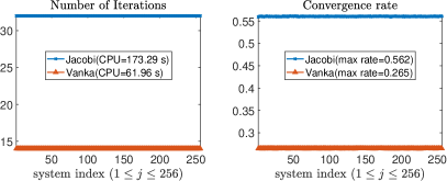
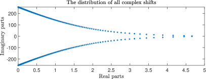
3.1 Example 1 (Heat equation).
In our first example, we test a PinT direct solver [3] for solving 2D heat equation, where the time discretization matrix (with a time step size ) is given by
| (9) |
It was shown in [3] that for all , which implies since . Figure 1 shows our proposed Vanka smoother is about 3 times faster than the Jacobi smoother, where the observed uniform convergence rates match well with the LFA prediction in Table 1.
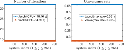
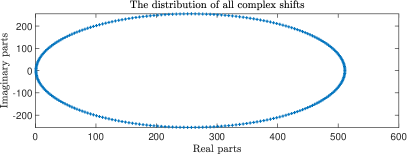
3.2 Example 2 (Backward heat conduction problem).
In our second example, we test a PinT quasi-boundary value method [20] for backward heat conduction problem, where the time discretization matrix (with a time step size ) reads
| (10) |
where is a small regularization parameter determined by the noise level . Figure 2 shows the same convergence rates, although the eigenvalues of leads to very different shifts.
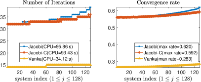
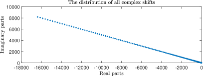
3.3 Example 3 (Isotropic Helmholtz equation).
In our third example, we test a sequence of 2D isotropic Helmholtz equation with the shifts given by with wavenumbers satisfying to avoid the pollution effect [12]. Here denotes the imaginary unit. Let ‘Jacobi-C’ denotes the damped Jacobi smoother with optimal complex relaxation parameter as proposed in [12]. Figure 3 shows our proposed Vanka smoother is about 3 times faster than both Jacobi and Jacobi-C smoother, where the Jacobi-C smoother outperforms the Jacobi smoother for large wavenumbers. The gradual deterioration of convergence rates for larger shifts is expected due to their negative real parts. The advantage of Jacobi-C smoother indicates our Vanka smoother may be further improved with carefully chosen complex relaxation parameter, which will be left as our future work.
4 Conclusions
In this paper we have proposed and analyzed an additive element-wise Vanka smoother for complex-shifted Laplacian systems that stem from a class of diagonalization-based PinT algorithms. Numerical results with various applications confirmed our theoretical outcomes based on LFA techniques. It is also possible to generalize our method to similar complex-shifted linear systems arising in the Laplace transform-based parallelizable contour integral method (see e.g., [21]).
References
- [1] M. J. Gander, 50 years of time parallel time integration, in: Multiple shooting and time domain decomposition methods, Springer, 2015, pp. 69–113.
- [2] M. J. Gander, J. Liu, S.-L. Wu, X. Yue, T. Zhou, ParaDiag: parallel-in-time algorithms based on the diagonalization technique, arXiv preprint arXiv:2005.09158 (2020).
- [3] J. Liu, X.-S. Wang, S.-L. Wu, T. Zhou, A well-conditioned direct pint algorithm for first-and second-order evolutionary equations, to appear in Advances in Computational Mathematics (arXiv preprint arXiv:2108.01716) (2021).
- [4] E. McDonald, J. Pestana, A. Wathen, Preconditioning and iterative solution of all-at-once systems for evolutionary partial differential equations, SIAM Journal on Scientific Computing 40 (2) (2018) A1012–A1033.
- [5] X. Lin, M. Ng, An all-at-once preconditioner for evolutionary partial differential equations, SIAM Journal on Scientific Computing 43 (4) (2021) A2766–A2784.
- [6] J. Liu, S.-L. Wu, A fast block -circulant preconditoner for all-at-once systems from wave equations, SIAM Journal on Matrix Analysis and Applications 41 (4) (2020) 1912–1943.
- [7] A. Goddard, A. Wathen, A note on parallel preconditioning for all-at-once evolutionary PDEs, Electron. Trans. Numer. Anal. 51 (2019) 135–150.
- [8] M. J. Gander, L. Halpern, J. Rannou, J. Ryan, A direct time parallel solver by diagonalization for the wave equation, SIAM Journal on Scientific Computing 41 (1) (2019) A220–A245.
- [9] Y. A. Erlangga, C. W. Oosterlee, C. Vuik, A novel multigrid based preconditioner for heterogeneous Helmholtz problems, SIAM Journal on Scientific Computing 27 (4) (2006) 1471–1492.
- [10] S. Cools, W. Vanroose, Local Fourier analysis of the complex shifted Laplacian preconditioner for Helmholtz problems, Numerical Linear Algebra with Applications 20 (4) (2013) 575–597.
- [11] P.-H. Cocquet, M. J. Gander, How large a shift is needed in the shifted Helmholtz preconditioner for its effective inversion by multigrid?, SIAM Journal on Scientific Computing 39 (2) (2017) A438–A478.
- [12] L. R. Hocking, C. Greif, Optimal complex relaxation parameters in multigrid for complex-shifted linear systems, SIAM Journal on Matrix Analysis and Applications 42 (2) (2021) 475–502.
- [13] C. Greif, Y. He, A closed-form multigrid smoothing factor for an additive Vanka-type smoother applied to the Poisson equation, arXiv preprint arXiv:2111.03190 (2021).
- [14] S. Vanka, Block-implicit multigrid calculation of two-dimensional recirculating flows, Computer Methods in Applied Mechanics and Engineering 59 (1) (1986) 29–48.
- [15] A. P. de la Riva, C. Rodrigo, F. J. Gaspar, A robust multigrid solver for isogeometric analysis based on multiplicative Schwarz smoothers, SIAM Journal on Scientific Computing 41 (5) (2019) S321–S345.
- [16] P. E. Farrell, Y. He, S. P. MacLachlan, A local Fourier analysis of additive Vanka relaxation for the Stokes equations, Numerical Linear Algebra with Applications 28 (3) (2020).
- [17] L. Claus, M. Bolten, Nonoverlapping block smoothers for the Stokes equations, Numerical Linear Algebra with Applications 28 (6) (2021).
- [18] R. Wienands, W. Joppich, Practical Fourier analysis for multigrid methods, CRC press, 2004.
- [19] U. Trottenberg, C. W. Oosterlee, A. Schuller, Multigrid, Academic press, 2000.
- [20] J. Liu, Fast parallel-in-time quasi-boundary value methods for backward heat conduction problems, arXiv preprint arXiv:2107.06381 (2021).
- [21] D. Sheen, I. H. Sloan, V. Thomée, A parallel method for time discretization of parabolic equations based on laplace transformation and quadrature, IMA Journal of Numerical Analysis 23 (2) (2003) 269–299.