Short Text Topic Modeling:
Application to tweets about Bitcoin

Abstract

Understanding the semantic of a collection of texts is a challenging task. Topic models are probabilistic models that aims at extracting ”topics” from a corpus of documents. This task is particularly difficult when the corpus is composed of short texts, such as posts on social networks. Following several previous research papers, we explore in this paper a set of collected tweets about bitcoin. In this work, we train three topic models and evaluate their output with several scores. We also propose a concrete application of the extracted topics.

I Introduction

Understanding the semantic of a collection of texts, or corpus, is a challenging task. Topic modeling provides a convenient way to analyze large collections of unstructured text, and are one of the most popular methods for learning representations of textual data. The increasing amount of data requires the use of unsupervised algorithms that learn meaningful patterns of words without requiring any prior annotations. From word co-occurrences, topics models aims at extracting topics from a set of documents, that is, groups of words that tend to appear together. Various hierarchical probabilistic graphical models such as Latent Dirichlet Allocation (LDA) [1], Probabilistic Latent Semantic Allocation (PLSA) [2], and hundreds of variants, have been introduced to this end. In PLSA and LDA, topics are distribution vectors over the vocabulary and documents consists of a mixture of topics.

Social networks, such as Reddit or Twitter, have become important communication tools for people, among retail investors. Previous studies show relations between social network data and performance of securities or other financial instruments [3, 4, 5, 6]. In particular, social networks are an important source of information for cryptocurrency users and investors. Data from social networks could be used to detect breaking news or trending projects. It is however worth pointing out that messages on those platforms are most often characterized by their lack of context and their flexible language. In addition, most of social networks are microblogging websites, e.g. messages on Twitter, or tweets, are restricted to 140 characters. As a consequence, we often have to deal with short texts. For all the above reasons, topic modeling on those kinds of datasets tends to be a daunting task.

Several works used standard topic models to model topics on short texts, but observed a severe degradation in the performances of those algorithms [7, 8, 9]. This is mainly due to the lack of co-occurrence information in short documents, indeed, short texts typically only include a few words. In order to overcome this problem of sparsity, new models such as Dirichlet Multinomial Mixture (DMM) [10], have been introduced [11, 12]. DMM is a simplication of the LDA model, in which each document is supposed to have been generated from only one topic instead of a mixture of topics. Recent studies suggest that DMM is more adapted to short texts than LDA and PLSA. Several research papers also propose models that incorporate metadata such as information about the author [13] or token embeddings [14, 15], but are out of the scope of this paper.

Prior to this work, we collected textual data from two data sources: tweets from prominent personalities of the Bitcoin community and messages posted on the specialized forum BitcoinTalk.org. The contribution of this article is to train three different models: LDA [1], prodLDA [16] and DMM [10] on the dataset of tweets, and to evaluate their performances on the Bitcoin Talk dataset. A model is said to be performing if the output topics are semantically coherent for humans. Since objective functions that are optimized by those models do not always correlate with human judgments of topic quality, we use several evaluation measures that have been explicitly developed to evaluate the coherence of models. As previously said, a trained topic model can be used to to find Euclidean representations of textual data. We finally show in this work that the representations found can be significant for predicting bitcoin’s future returns.

II Data

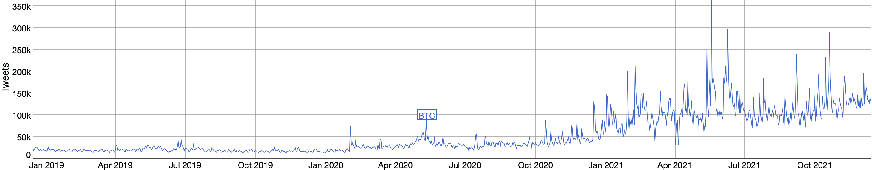
Figure 1: Number of tweets mentioning ”btc” or ”bitcoin” (source: https://bitinfocharts.com).

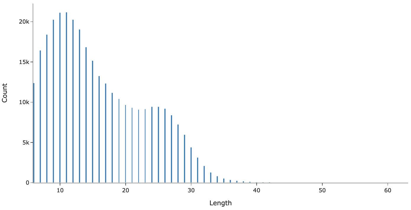
Figure 2: Twitter: histogram of length.

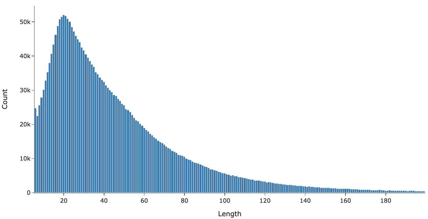
Figure 3: Bitcoin Talk: histogram of length.

Prior to this work, we collected two datasets of texts from social networks : first, a set of tweets of prominent Twitter accounts in the cryptocurrency community and secondly, a set of messages posted on the forum Bitcoin Talk.

Twitter

Twitter (https://twitter.com) is a popular microblogging and social networking service on which people can post and interact with short messages, namely tweets. Bitcoin community and more generally cryptocurrency communities are very established on Twitter. Figure 1 shows that the daily volume of tweets mentioning ”bitcoin” has been increasing steadily since 2019. The number of tweets published about Bitcoin can culminate up to several hundreds of thousand each day. The huge quantity of tweets published each day makes it difficult to collect all of them. In addition, most of these tweets can be considered as spam [17], or are not likely to have an influence on the propagation of news. We decide first to establish a list of prominent accounts of the Bitcoin community, and, then, to collect all tweets from these accounts. To this end, we collect all tweets mentioning ”btc” or ”bitcoin” and having generated more than 5000 retweets from the 30th June 2017 to the 30th June 2021. Next, we filter out accounts that are present less than 5 times in order not to take into account accounts that were sporadically viral. Finally, we collect all tweets mentioning ”btc” or ”bitcoin” from the remaining accounts, this time without restriction on the number of retweets.

Bitcoin Talk

Bitcoin Talk (https://bitcointalk.org) is one the most popular online forum dedicated to cryptocurrency and blockchain technology. In particular, people can ask questions and discuss topics related to Bitcoin. The forum was even created by the creator of Bitcoin itself, Satoshi Nakamoto. There are several sections in which several thousands of discussions, or threads, are available. We collect all messages published in the following sections : ”Bitcoin Discussion”, ”Economics”, ”Gambling”, ”Speculation”, ”Securities”, ”Press”, ”Trading discussion” and ”Legal”, from the 22th November 2009 to the 30th Mai 2021.

We report in table I several statistics on both datasets. In figures 3 and 3 we plot histograms of the length of the collected tweets and messages on Bitcoin Talk, respectively. We observe that tweets are globally shorter than messages on Bitcoin Talk. The dataset Twitter will be used to train our models and the dataset Bitcoin Talk will be used to select the best model, as evaluation metrics are more reliable with longer texts.

Dataset	Documents	Authors	Threads
Twitter	328055	310	/
Bitcoin Talk	2552937	92193	46614

TABLE I: Dataset statistics

III Methods

Notations:

• $\mathcal{D}$ the training corpus

• $N_{d}\triangleq|\mathcal{D}|$ the number of documents

• $K\in\mathbb{N}$ the number of topics

• $V\in\mathbb{N}$ the vocabulary size

• $\Delta(n)\triangleq\{\mathbf{p}\in\mathbb{R}^{n},\ \mathbf{p}\geq 0,\ \sum_{i=1}^{n}p_{i}=1\}$

• $\sigma$ the softmax function

• $\mathrm{diag}(V)$ is the diagonal matrix whose diagonal is equal to $V$

In this section, we will discuss some of the topic modeling methods that deals with words, documents and topics. All the studied models make the Naive Bayes assumption, i.e. words in a document are generated independently.

III-A Dirichlet Multinomial Mixture

III-A1 Model

Dirichlet Multinomial Mixture (DMM) is a generative probabilistic model in which each document covers an unique topic. This model was introduced by Yin and Wang in [10]. It is parametrized by two vectors $\boldsymbol{\alpha}\in(\mathbb{R}^{+*})^{K}$ and $\boldsymbol{\beta}\in(\mathbb{R}^{+*})^{V}$ defining two Dirichlet priors. We suppose that these priors are symmetric, i.e. $\boldsymbol{\alpha}\propto\overrightarrow{1}$ and $\boldsymbol{\beta}\propto\overrightarrow{1}$, this assumption implies that all topics and words are equally important in the beginning. In the following, we will denote by $\alpha$ and $\beta$ the real numbers satisfying $\boldsymbol{\alpha}=\alpha\cdot\overrightarrow{1}$ and $\boldsymbol{\beta}=\beta\cdot\overrightarrow{1}$. Hyper-parameters $\alpha$ and $\beta$ can be here easily interpreted through an analogy, see the reference [10] for further details. A corpus is characterized by a topic probability distribution $\boldsymbol{\theta}\in\Delta(K)\sim\mathrm{Dirichlet}(\boldsymbol{\alpha})$, $\theta_{t}$ is the asymptotic proportion of documents covering topic $t$. In addition, each topic $t$ is characterized by a probability vector $\boldsymbol{\phi_{t}}\in\Delta(V)$ over the vocabulary, the $\boldsymbol{\phi_{1}},...,\boldsymbol{\phi_{K}}$ are i.i.d samples from $\mathrm{Dirichlet}(\boldsymbol{\beta})$. The generative process of a new document $d$ is defined as follows: first a topic $z$ is sampled from $\mathrm{Multinomial}(1,\boldsymbol{\theta})$, then $N$ words $\{w_{1},...,w_{N}\}$ are i.i.d sampled from $\mathrm{Multinomial}(1,\boldsymbol{\phi_{z}})$. This graphical model is represented on figure 4 and the generative process on algorithm 1.

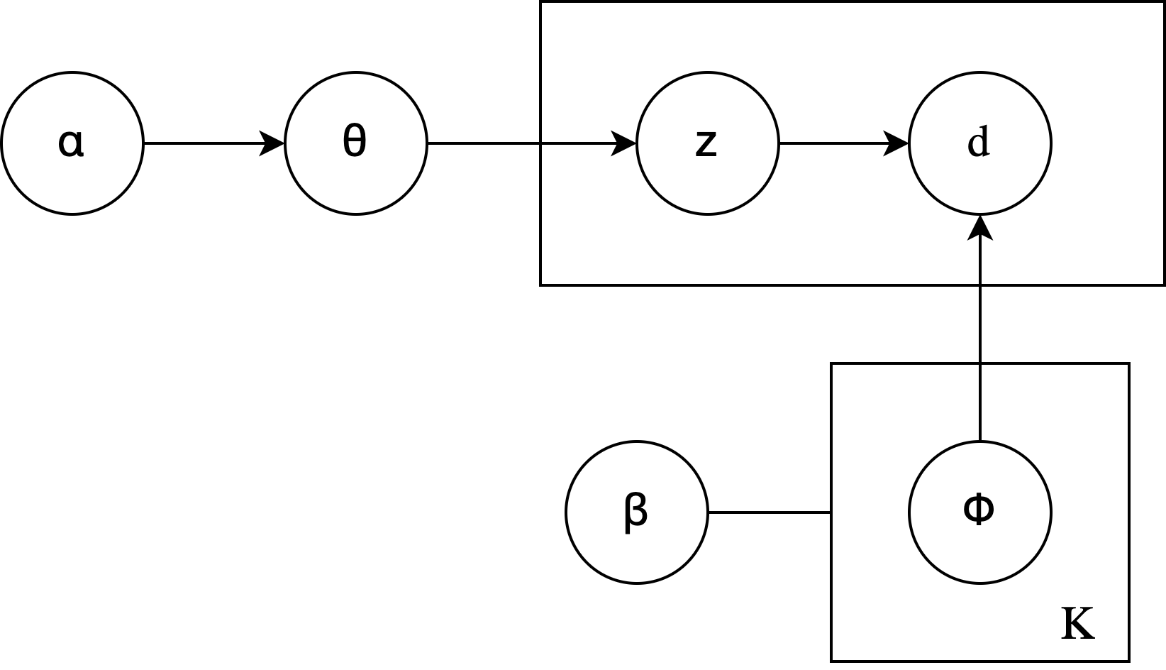
Figure 4: Graphical Model of DMM.

Data: $N\in\mathbb{N}$

Result: Document $d$

$z\sim\mathrm{Multinomial}(1;\boldsymbol{\alpha})$;

$d\sim\mathrm{Multinomial}(N;\boldsymbol{\phi_{z}})$;

Algorithm 1 DMM: generative process of new documents.

The joint probability of this graphical model therefore satisfies :

$$\small p(d,\alpha,\beta,z,\boldsymbol{\phi},\boldsymbol{\theta})=p(\alpha)p(\boldsymbol{\theta}|\alpha)p(z|\boldsymbol{\theta})p(d|z,\boldsymbol{\phi})p(\boldsymbol{\phi}|\beta)p(\beta)$$ (1)

where the probability of $d$ conditioned on $\boldsymbol{\theta}$ and $\boldsymbol{\phi}$ is:

$$\small\begin{split}p(d|\boldsymbol{\theta},\boldsymbol{\phi})&=\sum_{z}p(d|z,\boldsymbol{\theta},\boldsymbol{\phi})p(z|\boldsymbol{\theta},\boldsymbol{\phi})\\ &=\sum_{z}p(d|z,\boldsymbol{\phi})p(z|\boldsymbol{\theta})\\ &=\sum_{z}\left(\prod_{w\in d}p(w|z,\boldsymbol{\phi})\right)\theta_{z}\\ &=\sum_{z}\left(\prod_{w\in d}\phi_{z,w}\right)\theta_{z}\\ \end{split}$$ (2)

III-A2 Inference

A corpus can be explored by examining the posterior distribution of $\boldsymbol{\phi}$, $\boldsymbol{\theta}$ and assignments $\mathbf{z}$ conditioned on the train documents. However the posterior cannot be computed directly [10]. We use the collapsed Gibbs sampling algorithm, a MCMC algorithm, introduced by Yin and Wang to approximate the posterior given the train corpus. $\alpha$ and $\beta$ are fixed at the beginning during the initialization. This method first initializes all topic labels randomly, next it iterates several times over the documents. For each document $d$, its new label is updated according to the conditional distribution $p(z_{d}|d,\{z_{d^{{}^{\prime}}}\}_{d^{{}^{\prime}}\in\mathcal{D}-\{d\}},\alpha,\beta)$.

III-A3 Estimation of the topic-word matrix

At the end of the training phase, each document $d$ has been assigned a label $z_{d}$. We introduce the following notations:

• $\mathcal{Z}\triangleq\{z_{d}\}_{d\in\mathcal{D}}$ the set of topic assignments,

• $\mathcal{D}_{i}\triangleq\{d\in\mathcal{D},\ z_{d}=i\}$ the set of documents covering topic $i$,

• $T_{i}\triangleq\sum_{d\in\mathcal{D}_{i}}|d|$ the total number of words of all documents covering topic $i$,

• $n^{T}_{i}\triangleq|\mathcal{D}_{i}|$ the number of documents covering topic $i$

• $n_{i,w}^{W}$ the number of occurence of $w$ in $\mathcal{D}_{i}$,

The posterior probability function of $\boldsymbol{\phi_{i}}$ given the documents and the inferred labels can be derived as follows:

$$\small\begin{split}p(\boldsymbol{\phi_{i}}|\mathcal{Z},\mathcal{D},\alpha,\beta)&\overset{(B)}{\propto}p(\mathcal{D}|\boldsymbol{\phi_{i}},\mathcal{Z},\alpha,\beta)p(\boldsymbol{\phi_{i}}|\mathcal{Z},\alpha,\beta)\\ &\overset{(AG)}{\propto}p(\mathcal{D}_{i}|\boldsymbol{\phi_{i}},\mathcal{Z})p(\boldsymbol{\boldsymbol{\phi_{i}}}|\beta)\\ &\overset{(AD)}{\propto}\mathrm{Multinomial}(\mathcal{D}_{i};T_{i},\boldsymbol{\phi_{i}})\mathrm{Dirichlet}(\boldsymbol{\phi_{i}};\boldsymbol{\beta})\\ &\overset{(A1)}{\propto}\mathrm{Dirichlet}(\boldsymbol{\phi_{i}};V,\boldsymbol{\beta}+\boldsymbol{n^{W}_{i}})\end{split}$$ (3)

where we use the following arguments : $(B)$ Bayes’ theorem, $(AG)$ structure of the graphical model, $(AD)$ hypothesis of DMM about conditional distributions and $(A1)$ the fact that Dirichlet distribution is conjugate to the multinomial distribution. Finally, $\boldsymbol{\phi_{i}}$ can be estimated by the mean $\boldsymbol{\hat{\phi}_{i}}$ of the posterior:

$$\small\boldsymbol{\hat{\phi}_{i}}=\left(\frac{\beta+n^{W}_{i,w}}{T_{i}+V\beta}\right)_{w=1,...,V}$$ (4)

By using the same kind of arguments,

$$\small\begin{split}p(\boldsymbol{\theta}|\mathcal{Z},\mathcal{D},\alpha,\beta)&\propto p(\mathcal{Z}|\boldsymbol{\theta})p(\boldsymbol{\boldsymbol{\theta}}|\alpha)\\ &\propto\mathrm{Multinomial}(\mathcal{Z};N_{d},\boldsymbol{\theta})\mathrm{Dirichlet}(\boldsymbol{\theta};\boldsymbol{\alpha})\\ &\propto\mathrm{Dirichlet}(\boldsymbol{\theta};K,\boldsymbol{\alpha}+\boldsymbol{n^{T}})\end{split}$$ (5)

$\boldsymbol{\theta}$ is approximated by $\boldsymbol{\hat{\theta}}$ the posterior mean:

$$\small\boldsymbol{\hat{\theta}}=\left(\frac{\alpha+n^{T}_{i}}{N+K\alpha}\right)_{i=1,...,K}$$ (6)

III-B Latent Dirichlet Allocation

III-B1 Model

Latent Dirichlet Allocation (LDA) is a generative probabilistic model introduced by Blei et al.[1] in which each document is represented as a mixture of topics in contrary to DMM for which only one topic is covered. As the DMM model, LDA is parametrized by $\boldsymbol{\alpha}\in(\mathbb{R}^{+*})^{K}$ and $\boldsymbol{\beta}\in(\mathbb{R}^{+*})^{V}$ defining two Dirichlet priors. Topics are characterized by $\{\boldsymbol{\phi_{1}},...,\boldsymbol{\phi_{K}}\}$ i.i.d sampled from $\mathrm{Dirichlet}(\boldsymbol{\beta})$. For generating a new document $d$, a topic distribution $\boldsymbol{\theta}$ is sampled from $\mathrm{Dirichlet}(\boldsymbol{\alpha})$. Then, for each word position $n$, we sample a topic $z_{n}$ from $\mathrm{Multinomial}(1,\boldsymbol{\theta})$ and a word $w_{n}$ according to $\mathrm{Multinomial}(1,\boldsymbol{\phi_{z_{n}}}$). As in DMM, we suppose that the Dirichlet priors are symmetric. This graphical model is represented on figure 5 and the generative process on algorithm 2.

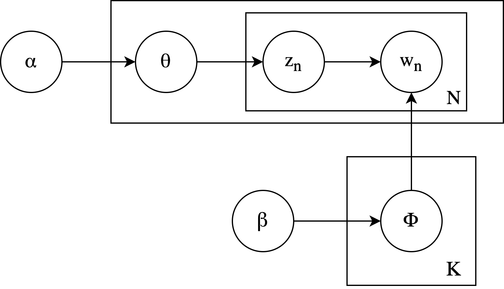
Figure 5: Graphical Model of LDA

Data: $N\in\mathbb{N}$

Result: Document $d=\{w_{1},...,w_{N}\}$

$\boldsymbol{\theta}\sim\mathrm{Dirichlet}(\boldsymbol{\alpha})$;

for $n=1,...,N$ do

       $z_{n}\sim\mathrm{Multinomial}(1;\boldsymbol{\theta})$;

       $w_{n}\sim\mathrm{Multinomial}(1;\boldsymbol{\phi_{z_{n}}})$;

      

end for

Algorithm 2 LDA : generative process of a new document.

The joint probability of this graphical model therefore satisfies :

$$\small p(d,\alpha,\beta,\mathbf{z},\boldsymbol{\phi},\boldsymbol{\theta})=p(\alpha)p(\boldsymbol{\theta}|\alpha)p(d|\mathbf{z},\boldsymbol{\phi})p(\mathbf{z}|\boldsymbol{\theta})p(\boldsymbol{\phi}|\beta)p(\beta)$$ (7)

Furthermore,

$$p(\mathbf{z}|\boldsymbol{\theta})p(d|\mathbf{z},\boldsymbol{\phi})=\prod_{i=1}^{N}p(w_{n}|z_{n},\boldsymbol{\phi})p(z_{n}|\boldsymbol{\theta})$$

The probability of $d$ conditioned on ${\alpha}$ and $\boldsymbol{\phi}$ is intractable, indeed:

$$\small\begin{split}p(d|\alpha,\boldsymbol{\phi})&=\int_{\Delta(K)}p(d|\alpha,\boldsymbol{\theta},\boldsymbol{\phi})p(\boldsymbol{\theta}|\alpha,\boldsymbol{\phi})\mathrm{d}\boldsymbol{\theta}\\ &=\int_{\Delta(K)}p(d|\boldsymbol{\theta},\boldsymbol{\phi})p(\boldsymbol{\theta}|\alpha)\mathrm{d}\boldsymbol{\theta}\\ &=\int_{\Delta(K)}\left(\prod_{w\in d}\sum_{z}p(w|z,\boldsymbol{\phi_{z}})p(z|\boldsymbol{\theta})\right)p(\boldsymbol{\theta}|\alpha)\mathrm{d}\boldsymbol{\theta}\end{split}$$ (8)

III-B2 Inference

As in DMM, the posterior distribution is intractable. The variational Bayes algorithm is traditionally used to this end. The true posterior is approximated by a simpler distribution $q(\boldsymbol{\phi},\boldsymbol{\theta},\boldsymbol{z}|\boldsymbol{\chi})$ with $\boldsymbol{\chi}$ a set of free parameters. Parameters $\boldsymbol{\chi}$ are optimized to maximise the Evidence Lower Bound, or shortly ELBO, quantity (equation 9).

$$\small\begin{split}\mathrm{ELBO}(\mathcal{D},\boldsymbol{\chi})&=\mathbb{E}_{q}(\log(p(\mathcal{D},\boldsymbol{z},\boldsymbol{\theta},\boldsymbol{\phi}|\alpha,\beta)))\\ &-\mathbb{E}_{q}(\log(q(\boldsymbol{z},\boldsymbol{\theta},\boldsymbol{\phi}|\boldsymbol{\chi})))\end{split}$$ (9)

As its name suggests, the ELBO is a lower bound of the loglikelihood of the observed data, i.e. the evidence:

$$\small\log(p(\mathcal{D}|\alpha,\beta))$$ (10)

In particular we use the online method introduced by Hoffman et al. [18].

III-B3 Estimation of the topic-word matrix

The online variational Bayes algorithm of Hoffman et al. allows to approximate the posterior of $\boldsymbol{\phi}$ conditioned on the corpus. $\boldsymbol{\phi}$ is finally estimated by the posterior mean.

III-C ProdLDA

III-C1 Model

First, it is worth noticing that topic assignments $\mathbf{z}$ in LDA can be collapsed by mixing the multinomial distributions:

$$\small\sum_{z}p(w|z,\boldsymbol{\phi})p(z,\boldsymbol{\theta})=\sum_{z}\phi_{z,w}\theta_{w}=(\boldsymbol{\phi}\times\boldsymbol{\theta})_{w}$$ (11)

Thus,

$$\small p(w|\boldsymbol{\phi},\boldsymbol{\theta})=\mathrm{Multinomial}(w;1,\boldsymbol{\phi}\times\boldsymbol{\theta})$$ (12)

The ProdLDA model is very similar to the LDA model. In ProdLDA, rows of the topic-word distribution matrix are not sampled from a Dirichlet distribution. Moreover, rows of $\boldsymbol{\phi}$ are not even constrained to live in $\Delta(V)$. Multinomial distributions are first mixed before being normalized into a distribution, that is:

$$\small\begin{split}p(w|\boldsymbol{\phi},\boldsymbol{\theta})&=\mathrm{Multinomial}(w;1,\sigma(\boldsymbol{\phi}\times\boldsymbol{\theta}))\\ &\propto\prod_{z}p(w|z,\boldsymbol{\phi_{z}})^{\theta_{z}}\end{split}$$ (13)

As a result, $w|\boldsymbol{\theta},\boldsymbol{\phi}$ is a weighted product of expert instead of a mixture of multinomial.

III-C2 Inference

Computing the posterior is here again intractable. As for LDA, we use a variational Bayes method in order to approximate the posterior distribution $p(\boldsymbol{\theta},\boldsymbol{\phi}|\mathcal{D},\alpha)$. Srivastava and Sutton [16] propose to use a Variational AutoEncoder (VAE), a deep neural network, to this end. A Variational AutoEncoder is composed of two successive modules : first the encoder, or inference network , and then the decoder. A document $d$ is fed to the encoder which outputs an approximation $q$ of the posterior distribution $p(\boldsymbol{\theta}|d)$. $q(\boldsymbol{\theta}|d)$ belongs then to a parametric family of distributions, and is parametrized by $\boldsymbol{\chi}$, the free parameters of the encoder. Next, a sample $\boldsymbol{\theta_{s}}$ of $q(\boldsymbol{\theta}|d,\chi)$ is fed to the decoder, which outputs a probability vector $p(w|\boldsymbol{\theta_{s}},\boldsymbol{\phi})$ over the vocabulary (equation 14).

$$\small p(w|\boldsymbol{\theta_{s}},\boldsymbol{\phi})=\sigma(\boldsymbol{\phi}\times\boldsymbol{\theta_{s}})$$ (14)

The decoder is thus composed of a linear layer without bias and a Softmax layer. Srivastava and Sutton derive from the ELBO of equation 9 an objective function $L$ (equation 15) to minimize. The parameter of the model $\{\boldsymbol{\chi},\boldsymbol{\phi}\}$ are then optimized by a standard gradient descent algorithm.

$$\small\begin{split}L(\boldsymbol{\chi},\boldsymbol{\phi}|d,\alpha)&=\underbrace{D_{KL}(q(\boldsymbol{\theta}|\boldsymbol{\chi},d)||p(\boldsymbol{\theta}|\alpha))}_{\text{(1)}}\\ &+\underbrace{\mathbb{E}_{\boldsymbol{\theta_{s}}\sim q(\boldsymbol{\theta}|\boldsymbol{\chi},d)}(-\log(p(d|\boldsymbol{\theta_{s}},\boldsymbol{\phi}))}_{\text{(2)}}\end{split}$$ (15)

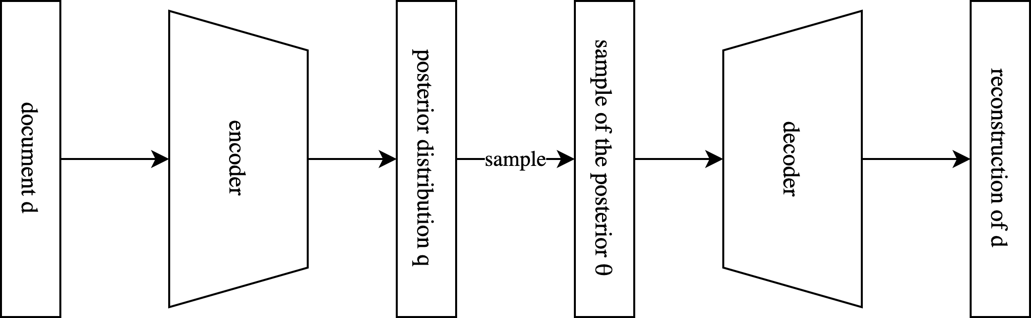
Figure 6: ProdLDA: Variational AutoEncoder

The term (1) of equation 15 is a regularization term which measures the difference between the approximate posterior distribution $q(\boldsymbol{\theta}|\boldsymbol{\chi},d)$ and the prior distribution $p(\boldsymbol{\theta}|\alpha)$. As a consequence, the approximate posterior is forced to stay close to the prior. The term (2) of equation 15 is a reconstruction error which aims to maximize the probability of the input document in our model.

The choice of the parametric family for $q$, i.e. the encoder, is crucial for two reasons:

• to derive a closed form of (1) in equation 15,

• to use the traditional Reparametrization Trick (RT) to sample from $q(\boldsymbol{\theta}|\boldsymbol{\chi},d)$,

Choosing a Dirichlet prior here is problematic because it does not allow to use the RT. To deal with this, Srivastava and Sutton use a Laplace approximation of the Dirichlet prior: $p(\boldsymbol{\theta}|\alpha)$ is approximated by $\hat{p}(\boldsymbol{\theta}|\boldsymbol{\tilde{\mu}},\boldsymbol{\tilde{\Sigma}})=\mathrm{LogNormal}(\boldsymbol{\theta};\boldsymbol{\tilde{\mu}},\boldsymbol{\tilde{\Sigma}})$, where $\boldsymbol{\tilde{\mu}}\in\mathbb{R}^{K}$ and $\boldsymbol{\tilde{\Sigma}}\in(\mathbb{R}^{+*})^{K}$ are computed from the parameter vector $\boldsymbol{\alpha}$ of the Dirichlet prior:

$$\small\tilde{\mu}_{k}=\log(\alpha_{k})-\frac{1}{K}\sum_{i}\log\alpha_{i}$$ (16)

$$\small\tilde{\Sigma}_{kk}=\frac{1}{\alpha_{k}}\left(1-\frac{2}{K}\right)+\frac{1}{K^{2}}\sum_{i}\frac{1}{\alpha_{k}}$$ (17)

The posterior $q$ is also approximated by a logistic normal distribution with a diagonal covariance matrix, i.e. $q(\boldsymbol{\theta}|\boldsymbol{\chi},d)=\mathrm{LogNormal}(\boldsymbol{\theta};\boldsymbol{\mu}(d),\mathrm{diag}(\boldsymbol{\Sigma}(d)))$ where $\boldsymbol{\mu}(d)\in\mathbb{R}^{K}$ and $\boldsymbol{\Sigma}(d)\in(\mathbb{R}^{+*})^{K}$ are the outputs of the encoder. As a consequence, we can rewrite (1) of equation 15 as:

$$\small\begin{split}D_{KL}(q(\boldsymbol{\theta}|\boldsymbol{\chi},d)||\hat{p}(\boldsymbol{\theta}|\boldsymbol{\alpha}))=\frac{1}{2}\bigg{(}\mathrm{tr}(\tilde{\boldsymbol{\Sigma}}^{-1}\boldsymbol{\Sigma}(d))\\ +(\boldsymbol{\tilde{\mu}}-\boldsymbol{\mu}(d))^{T}\boldsymbol{\Sigma}^{-1}(\boldsymbol{\tilde{\mu}}-\boldsymbol{\mu}(d))-K+\log\left(\frac{|\tilde{\boldsymbol{\Sigma}}|}{|\boldsymbol{\Sigma}(d)|}\right)\bigg{)}\end{split}$$ (18)

RT can be used with logistic normal distribution, indeed if $\boldsymbol{\epsilon}$ is sampled from $\mathrm{Normal}(0,\boldsymbol{I})$, then:

$$\small\sigma\left(\boldsymbol{\mu}+\sqrt{\mathrm{diag}(\boldsymbol{\Sigma})}\boldsymbol{\epsilon}\right)\sim\mathrm{LogitNormal}(\boldsymbol{\theta};\boldsymbol{\mu},\mathrm{diag}(\boldsymbol{\Sigma}))$$ (19)

Finally, the expected value of term (2) of equation 15 is approximated by a Monte Carlo estimator with one sample:

$$\small\begin{split}\mathbb{E}_{\boldsymbol{\theta}\sim q(\boldsymbol{\chi},d)}\left(-p(d|\boldsymbol{\theta},\boldsymbol{\phi})\right)\approx\\ -\sum_{w}1_{w\in d}\log\left(\sigma\left(\boldsymbol{\phi}\times\sigma\left(\boldsymbol{\mu}(d)+\sqrt{\boldsymbol{\Sigma}(d)}\boldsymbol{\epsilon}\right)\right)\right),\end{split}$$ (20)

where $\boldsymbol{\epsilon}\sim\mathrm{Normal}(0,\boldsymbol{I})$

III-C3 Estimation of the topic-word matrix

$\boldsymbol{\phi_{i}}$ is obtained by applying the Softmax function to the $i$-th row of the weight matrix $\boldsymbol{\phi}$ of the decoder.

IV Evaluation metrics

In the different models, a topic $i$ is defined by a distribution vector $\boldsymbol{\phi_{i}}$. A topic can thus be described its the most frequent words, or equivalently words with the highest probability. Intuitively, a subject is good if its top words are semantically coherent, that is, these words are meaningful enough so that a human can easily understand the main theme. Semantic coherence is subject to human subjectivity and judgement, and is therefore difficult to evaluate automatically. In this section, we present some metrics that are traditionally used to evaluate and select topic models.

IV-A Human judgement

As previously said, even if it may differ from one person to another, human judgment is the gold standard. To this end, human experts usually explore the set of top words by frequency in each topic. However, it may not be the best reduction technique for visualizing the topics and evaluating their quality. Indeed, overrepresented words such as ”btc” or ”bitcoin” are very likely to be top words for all topics, but do not give much information about the semantic of the topic. Arising out of this concern, Sievert and Shirley [19] introduce the relevance score $r$. The relevance $r_{\lambda}(w,i)$ of word $w$ for topic $i$ is computed as follow:

$$\small r_{\lambda}(w,i)=\lambda\log(\phi_{i,w})+(1-\lambda)\log\left(\frac{\phi_{w,i}}{p_{w}}\right)$$ (21)

where $\lambda\in[0,1]$ and $p_{w}$ is the empirical probability of $w$ in the corpus. If $\lambda=1$, ordering by topic-relevance is equivalent to ordering by topic-frequency. In contrary, if $\lambda=0$, importance is given to words essentially only present in this topic. $\lambda$ is therefore a tradeoff parameter, Sievert and Shirley recommend to set $\lambda$ equal to 0.3.

IV-B Perplexity

Let $\mathcal{D}^{(\mathrm{test})}$ a set of $N^{(\mathrm{test})}$ new documents $\{d_{1},d_{2},...,d_{N^{(\mathrm{test})}}\}$ generated with the same model as $\mathcal{D}$ was. Let $\mathcal{L}$ be the log likelihood function of our generative model. We can measure the quality of our model by evaluating the likelihood of the new document set $\mathcal{D}^{(\mathrm{test})}$, or perplexity. A high likelihood, or equivalently a high log-likelihood, would mean that our model is not surprised by the new documents, that is, the model has been quite good calibrated on the corpus $\mathcal{D}$. Since we supposed that documents are independently generated, we can decompose the log likelihood of the set into a sum of document log likelihood functions:

$$\small\mathcal{L}(\mathcal{D}^{(\mathrm{test})}|\mathcal{D})=\log p(\mathcal{D}^{(\mathrm{test})}|\mathcal{D})=\sum_{i=1}^{N^{(\mathrm{test})}}\log p(d_{i}|\mathcal{D})$$ (22)

Perplexity score is defined as follows:

$$\small\mathrm{perplexity}(\mathcal{D}^{(\mathrm{test})})=\exp\left(-\frac{\mathcal{L}(\mathcal{D}^{(\mathrm{test})}|\mathcal{D})}{\sum_{i=1}^{N^{(\mathrm{test})}}|d_{i}|}\right)$$ (23)

The lower the perplexity is, the better the model is assumed to be. It has been shown that perplexity is not a good metric for qualitative evaluation of topics [20], it is not strongly correlated to human judgement, and sometimes even negatively correlated. However, we will use it to select hyper-parameters of our DMM and LDA models.

For DMM, the log likelihood of an unseen document can be computed with equation 2 by remplacing $(\boldsymbol{\theta},\boldsymbol{\phi})$ by $(\boldsymbol{\hat{\theta}},\boldsymbol{\hat{\phi}})$ (equations 6 and 4). $\mathcal{L}(\mathcal{D}^{(\mathrm{test})}|\mathcal{D})$ is intractable for LDA and ProdLDA. Following Blei et al. [1], for variational methods we use the ELBO as a proxy for $\mathcal{L}(\mathcal{D}^{(\mathrm{test})}|\mathcal{D})$. For LDA, ELBO is computed by helding the topic matrix $\boldsymbol{\phi}$ fixed and fitting the free parameters over the topic distributions and topic assignments of new documents with the inference algorithm of [18]. For ProdLDA, new documents are fed to the VAE and ELBO is computed from equations 15, 18 and 19.

IV-C Coherence measures

Each topic $i$ can be represented by its most frequent words according to $\boldsymbol{\phi_{i}}$. Given a topic $i$, we denote by $w_{i}^{(1)},w_{i}^{(2)},...,w_{i}^{(V)}$ the words sorted by their frequencies in the descending order. Topic coherence measures take the set of $N$ top words of a topic and sum a confirmation measure over all word pairs. Once the confirmation measure is computed for all topics, they are aggregated into an unique coherence score. Several confirmation measures exist and we will study three of them in this section. UMass coherence is introduced by Mimno et al. [21] and, given a set of document $\mathcal{D}$, UMass for topic $i$ is computed as follows:

$$\small C_{UMass,i}=\frac{2}{N(N-1)}\sum_{m=2}^{N}\sum_{n=1}^{m-1}\log\left(\frac{p_{\mathcal{D}}(w_{i}^{(m)},w_{i}^{(n)})+\epsilon}{p_{\mathcal{D}}(w^{(n)})}\right)$$ (24)

where $\epsilon\approx 0^{+}$ is a small positive constant used to prevent numerical issues. The probability of a single word $p_{\mathcal{D}}(w)$ is defined as the number of documents of $\mathcal{D}$ in which the word $w$ occurs divided by the number of documents (equation 25). The joint probability of two words $p_{\mathcal{D}}(w_{1},w_{2})$ is estimated by the number of documents containing both words divided by the number of documents (equation 26).

$$\small p_{\mathcal{D}}(w)=\frac{\sum_{d\in\mathcal{D}}1_{w\in d}}{|\mathcal{D}|}$$ (25)

$$\small p_{\mathcal{D}}(w_{1},w_{2})=\frac{\sum_{d\in\mathcal{D}}1_{w_{1}\in d}1_{w_{2}\in d}}{|\mathcal{D}|}$$ (26)

Let $\omega\in\mathbb{N}$ be a window size. We denote by $\mathcal{D}_{\omega}$ the set of documents obtained by sliding a window of size $\omega$ over all documents of $\mathcal{D}$. UCI coherence for topic $i$ uses a confirmation based on pointwise mutual information (PMI) and is calculated by:

$$\small C_{UCI,i}=\frac{2}{N(N-1)}\sum_{m=1}^{N-1}\sum_{n=m+1}^{N}\mathrm{PMI}\left(w_{i}^{(m)},w_{i}^{(n)}\right)$$ (27)

with

$$\small\mathrm{PMI}\left(w_{i}^{(m)},w_{i}^{(n)}\right)=\log\left(\frac{p_{\mathcal{D}_{\omega}}\left(w_{i}^{(m)},w_{i}^{(n)}\right)+\epsilon}{p_{\mathcal{D}_{\omega}}\left(w_{i}^{(m)}\right)p_{\mathcal{D}_{\omega}}\left(w_{i}^{(n)}\right)}\right)$$ (28)

where probabilities in equation 28 are estimated on the set $\mathcal{D}_{\omega}$. NPMI coherence is obtained from the formula of UCI coherence by remplacing the PMI with the normalized log-ratio measure (NPMI) [22].

$$\small C_{NPMI,i}=\frac{2}{N(N-1)}\sum_{m=1}^{N-1}\sum_{n=m+1}^{N}\mathrm{NPMI}\left(w_{i}^{(m)},w_{i}^{(n)}\right)$$ (29)

$$\small NPMI(w_{i}^{(m)},w_{i}^{(n)})=\frac{PMI(w_{i}^{(m)},w_{j}^{(n)})}{-\log(p_{\mathcal{D}_{\omega}}(w_{i}^{(m)},w_{i}^{(n)})+\epsilon)}$$ (30)

Finally, coherence scores over all topics are aggregated by averaging.

$$\small C_{\cdot}=\frac{1}{K}\sum_{i=1}^{K}C_{\cdot,i}$$ (31)

Röder et al. [23] show that these coherence measures are strongly positively correlated with human ratings.

V Materials and Results

V-A Pre-processing

The pre-processing of both datasets involves the following steps:

1. removal of non-Latin characters / emojis / urls,

2. removal of mentions of other users, typically ”@user” in tweets,

3. removal of English stop words and punctuation,

4. lemmatization

5. tokenization

6. (DMM) removal of duplicate tokens

Finally, words that are present less than 100 times in the corpus are also removed. For steps 3 and 4, we use the Python package spaCy (https://spacy.io) with the english pipeline (https://spacy.io/models/en).

V-B Training

In this section, we train the models presented in section III on the dataset Twitter. Since the optimal number of topics is not known a priori, models are trained for a number of topics $K$ varying in $\{5,10,15,20,25,30,35,40,45,50\}$.

The model DMM is trained with a Gibbs sampling algorithm presented in III-A2, in particular we use the implementation of the Python package gsdmm (https://github.com/rwalk/gsdmm). Hyper-parameters $\alpha$ and $\beta$ are optimized by a 5-fold cross-validated grid-search over the parameter grid $[0.01,0.025,0.05,0.1,0.2]\times[0.06,0.1,0.24]$. Perplexity (equation 22) is used to score the goodness-of-fit of the model.

The model LDA is trained with a variational online algorithm presented in section III-B2. We use the popular Python package Gensim (https://radimrehurek.com/gensim/) for this purpose. Hyper-parameters $\kappa$ (decay) and $\tau_{0}$ (offset) are optimized by a 5-fold cross-validated grid search over the parameter grid $[0.6,0.75,0.9]\times[1,64,256]$. Perplexity, via its lower bound ELBO, is also used to select the best model.

The inference neural network of the VAE for ProdLDA is composed of three modules. The first module consists in two successive linear layers with Softplus activation, through which a document $d$ is summarized into a low-dimensional representation $\mathbf{z}$. Two parallel linear layers then transform $\mathbf{z}$ into the posterior mean $\boldsymbol{\mu}(d)$ and posterior log-variance $\log(\boldsymbol{\Sigma}(d))$. In accordance with equation 20, the decoder is composed of a linear layer without bias and a $\mathrm{Softmax}$ layer. We use $\mathrm{BatchNorm}$ and $\mathrm{Dropout}$ layers to facilitate the training. The encoder and decoder are represented in figures 7 and 8, respectively. The training data is split into a train (70%) and a validation (30%) set. We use the algorithm Adam with a learning rate of 0.001 and a batch size of 256 to minimize the objective function defined by equation 15. The training lasts at most 100 epochs, and is stopped if overfitting is detected in the evolution of validation loss.

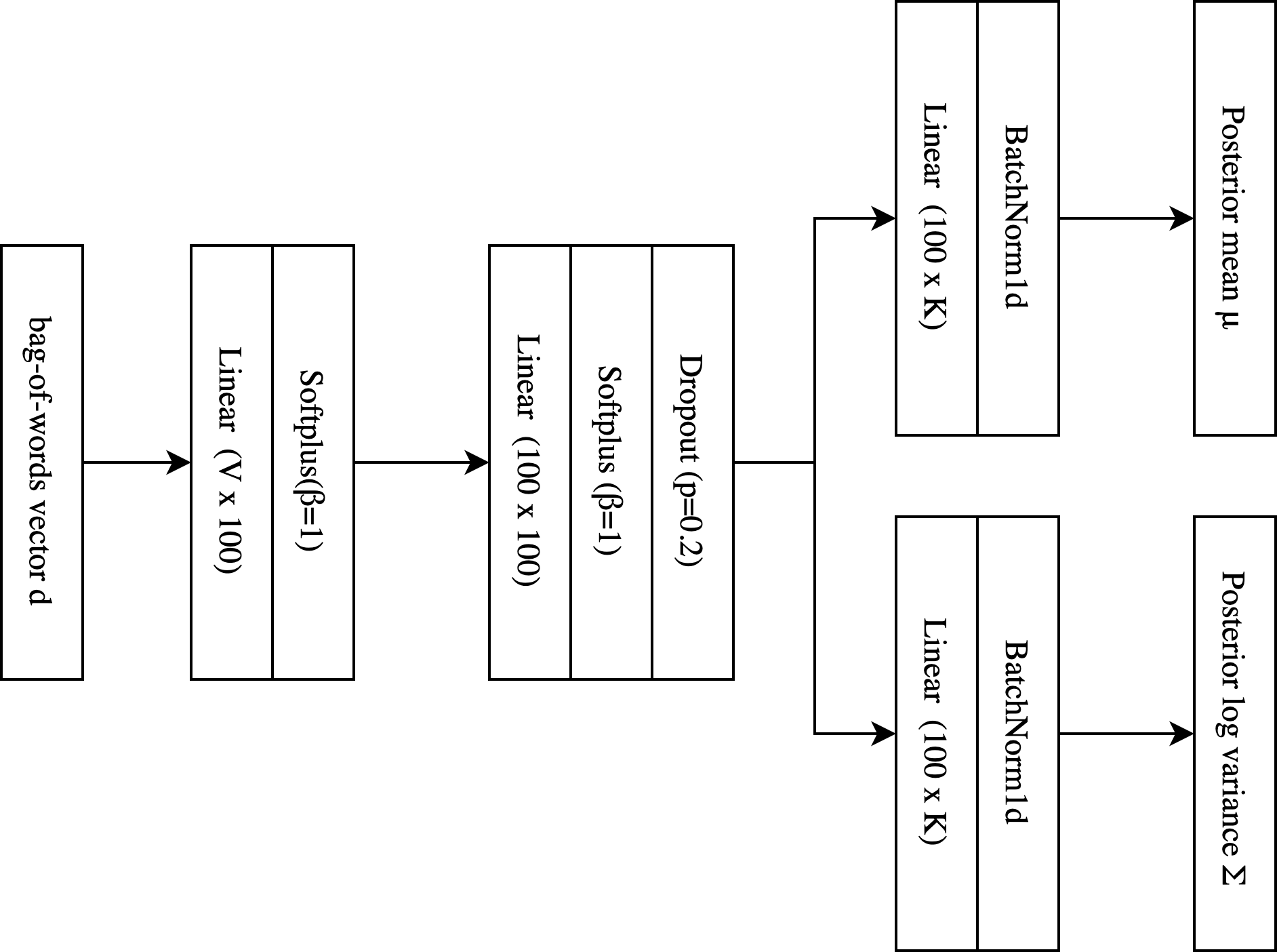
Figure 7: ProdLDA : inference network.

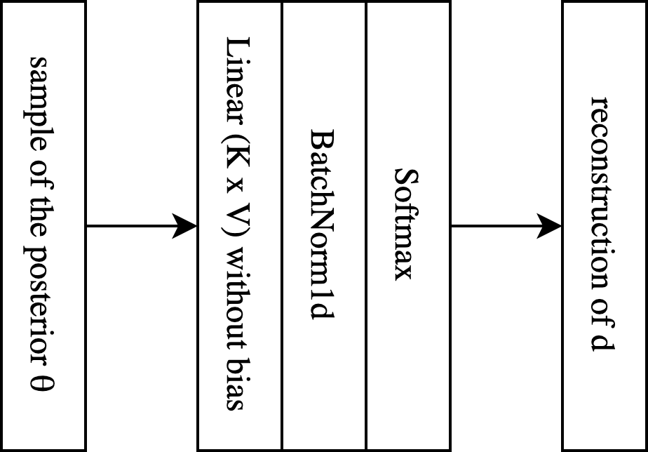
Figure 8: ProdLDA : decoder network.

V-C Evaluation

As stated in the introduction, documents in the corpus Bitcoin Talk are globally longer that those in the dataset Twitter. For this reason, this corpus is more suitable for evaluating the different models. We use the coherence scores $U_{MASS}$, $U_{UCI}$ and $U_{NPMI}$ presented in section 22. The scores are calculated with $N=20$ and $w=20$ for $U_{UCI}$ and $U_{NPMI}$. Scores are reported in tables IV, IV and IV, and in figures 11, 11 and 11.

K	DMM	LDA	prodLDA
5	-2.105	-2.779	-3.968
10	-2.225	-3.560	-3.257
15	-2.389	-3.590	-3.277
20	-2.127	-4.008	-3.044
25	-2.449	-4.157	-2.856
30	-2.468	-4.115	-2.845
35	-2.571	-4.347	-3.404
40	-2.588	-4.422	-3.293
45	-2.542	-4.193	-3.332
50	-2.630	-4.392	-3.328
Mean	$\mathbf{-2.408}$	-3.956	-3.260

TABLE II: $U_{MASS}$ coherence
on dataset Bitcoin Talk.

K	DMM	LDA	prodLDA
5	0.105	0.129	-0.286
10	0.325	0.212	0.254
15	0.522	0.180	0.417
20	0.545	0.101	0.361
25	0.492	0.062	0.378
30	0.407	0.056	0.336
35	0.422	0.027	0.330
40	0.373	-0.117	0.336
45	0.391	-0.132	0.329
50	0.354	-0.199	0.313
Mean	$\mathbf{0.394}$	0.032	0.277

TABLE III: $U_{UCI}$ coherence
on dataset Bitcoin Talk.

K	DMM	LDA	prodLDA
5	0.017	0.028	0.011
10	0.039	0.042	0.044
15	0.050	0.038	0.055
20	0.053	0.035	0.049
25	0.047	0.033	0.047
30	0.042	0.020	0.046
35	0.049	0.025	0.050
40	0.047	0.018	0.049
45	0.048	0.016	0.047
50	0.045	0.017	0.050
Mean	0.044	0.027	$\mathbf{0.045}$

TABLE IV: $U_{NPMI}$ coherence
on dataset Bitcoin Talk.

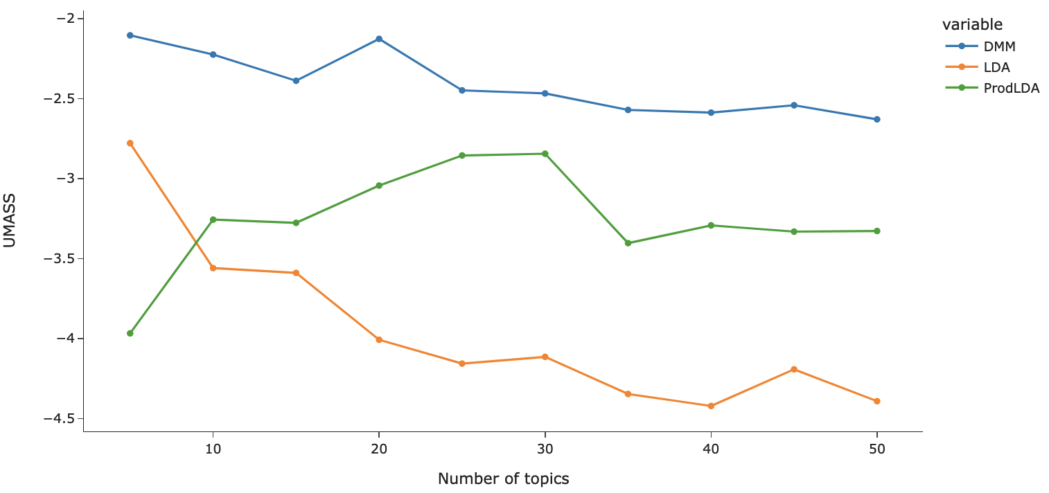
Figure 9: $U_{MASS}$ coherence on dataset Bitcoin Talk.

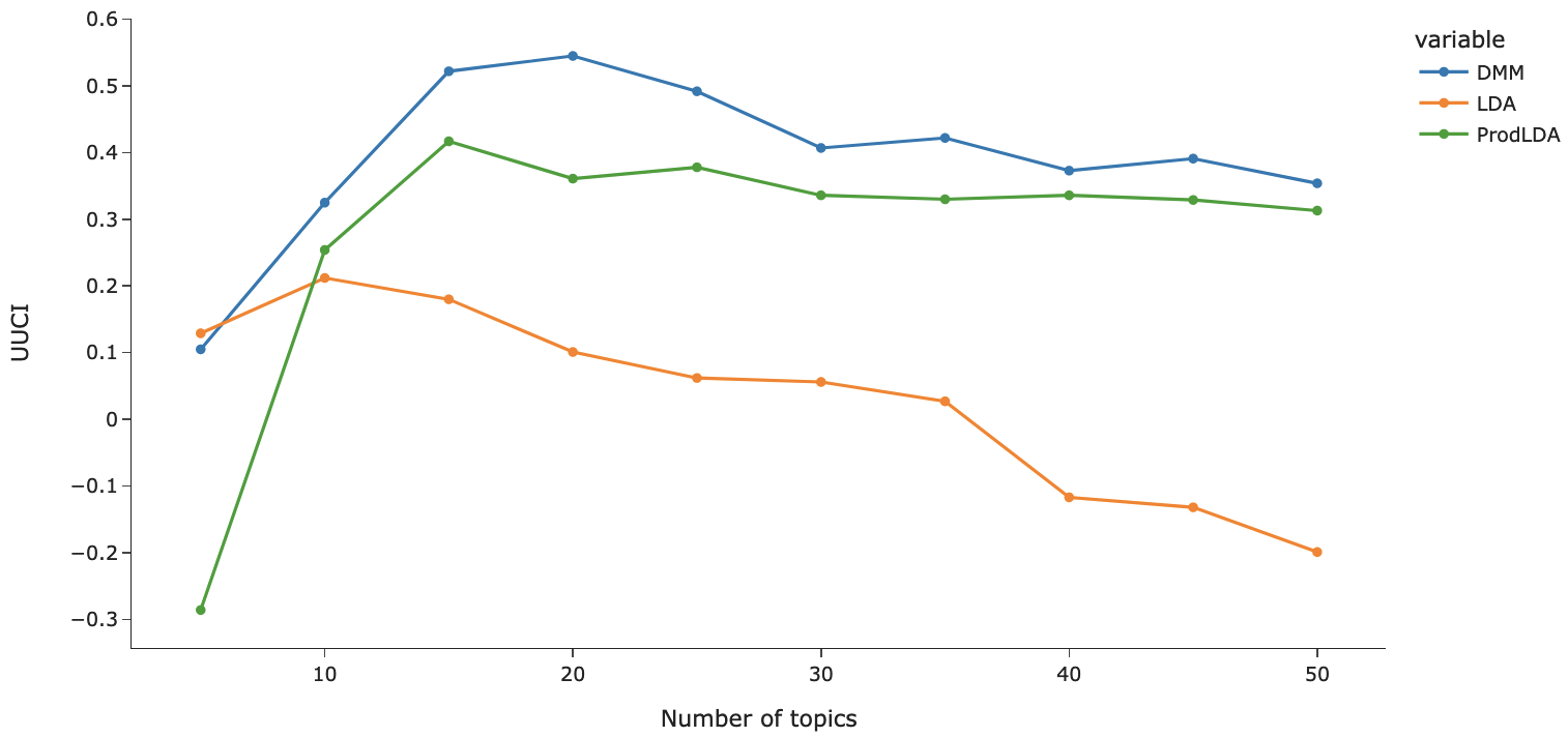
Figure 10: $U_{UCI}$ coherence on dataset Bitcoin Talk.

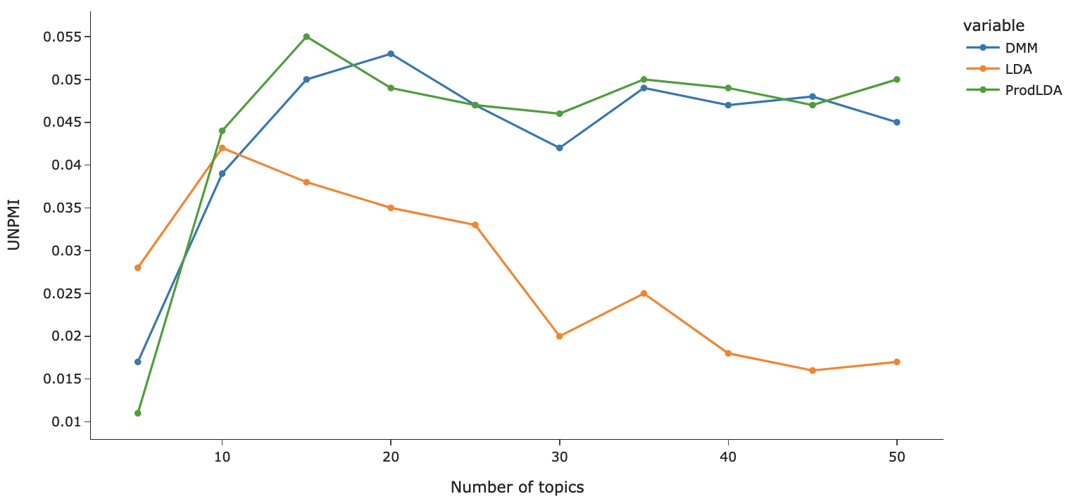
Figure 11: $U_{NPMI}$ coherence on dataset Bitcoin Talk.

In table V, we report for the model DMM trained on $K=20$ topics the top words for each cluster according to the relevance score introduced in section IV-A with $\lambda$ equal to 0.3.

Topic	Top words
0	maximalist, people, bitcoin, understand, scam, toxic, bitcoiner, think, shitcoin, criticism
1	friend, family, guy, dad, dinner, tell, buy, wife, pizza, man, girl
2	dump, panic, pump, sell, buy, fomo, crash, market, whale, btc
3	system, freedom, government, monetary, central, money, society, human, opt, nation
4	alt, profit, btc, trade, position, long, altcoin, pair, leverage, loss
5	rsi, resistance, daily, close, div, candle, hourly, bearish, bullish, bounce
6	value, layer, sov, store, settlement, censorship, utility, programmable, resistant, moe
7	s2f, asset, correlation, gold, sandp, stock, model, correlate, return, flow
8	episode, podcast, host, magazine, discuss, join, speaker, guest, topic, live
9	withdraw, pay, card, merchant, convert, ira, load, bitpay, payment, taxis
10	debt, print, fed, inflation, purchasing, rate, trillion, central, estate, bond
11	wallet, node, lightning, coinjoin, electrum, privacy, tor, hardware, wasabi, server
12	fork, consensus, segwit, segwit2x, contentious, uasf, reorg, core, pow, block
13	tender, legal, salvador, court, ban, india, wright, china, police, orea
14	upwards, breakout, resistance, area, zone, retest, diagonal, continuation, triangle, btcusd
15	cycle, precede, bull, correction, halve, retrace, prior, halving, historically, ath
16	inflow, outflow, volume, bitmex, gbtc, premium, exchange, greyscale, whale, bitfinex
17	renewable, mining, energy, electricity, miner, difficulty, hydro, hash, solar, subsidy
18	tudor, stanley, sachs, goldman, manager, jones, paul, blackrock, fund, morgan
19	musk, microstrategy, tesla, elon, sheet, dorsey, balance, square, saylor, jack

TABLE V: Model: DMM. $K=20$ topics. Top words according to the relevance score of equation 21 with $\lambda=0.3$.

V-D Application

In this section, we study the predictability of bitcoin returns with data from Twitter. In order to use traditional machine learning algorithms, we first have to find an Euclidean representation of each tweet. We set the number of topics $K$ equal to 20 and train the DMM with the optimal hyper-parameters $\alpha$ and $\beta$ found in section 8. We recall that a tweet is assigned to only one topic in this model. For this reason, one-hot encoding is a natural choice to construct a tweet representation $t_{\mathrm{tweet}}\in\{0,1\}^{K}$ as follows: for all $i\in\{0,1,2,...,K-1\}$, $t_{\mathrm{tweet},i}=1$ if $i$ is the topic label of the tweet and 0 otherwise. In several previous studies, it has been demonstrated that sentiment of tweets could also give information about future movements of bitcoin market. To complete this application, we extend the representation $t_{\mathrm{tweet}}$ with two sentiment scores: a positive sentiment $p_{\mathrm{tweet}}\in[0,1]$ and a negative sentiment $n_{\mathrm{tweet}}\in[0,1]$, both are computed with the Python package Vader (https://github.com/cjhutto/vaderSentiment). $p_{tweet}$ and $n_{tweet}$ are ratios for proportions of text that fall in positive and negative vocabulary, respectively. In this application, we seek to predict the next daily return $r_{d+1}$ of bitcoin relatively to the token USDT from the set of tweets $\mathcal{T}_{d}$ published on day $d$. Quotes have been downloaded from the Binance API. For each day $d$, we compute a topic vector $t_{d}$ by averaging topic vectors over all tweets in $\mathcal{T}_{d}$ (equation 32), we do the same to compute two average sentiment scores $p_{d}$ and $n_{d}$ (equations 33 and 34).

$$\small t_{d}=\frac{\sum_{\mathrm{tweet}\in\mathcal{T}_{d}}t_{\mathrm{tweet}}}{|\mathcal{T}_{d}|}$$ (32)

$$\small p_{d}=\frac{\sum_{\mathrm{tweet}\in\mathcal{T}_{d}}p_{\mathrm{tweet}}}{|\mathcal{T}_{d}|}$$ (33)

$$\small n_{d}=\frac{\sum_{\mathrm{tweet}\in\mathcal{T}_{d}}n_{\mathrm{tweet}}}{|\mathcal{T}_{d}|}$$ (34)

$t_{d}$ is thus the empirical distribution of inferred subjects of tweets published within the day $d$. $p_{d}$ and $n_{d}$ are the average ratios of positivity and negativity in the tweets. We train a linear regression model and report the results of the regression in table VI, in particular the p-values of significance t-tests for the different variables involved in the model.

Name	variable	coef.	std. err.	t-stat	p-value
Positive sentiment $**$	$p_{d}$	$0.200$	$0.041$	$4.819$	$0.000$
Negative sentiment $**$	$n_{d}$	-0.249	0.047	-5.317	0.000
Topic 0 ${**}$	$t_{d,0}$	0.040	0.009	4.263	0.000
Topic 1 ${**}$	$t_{d,1}$	0.097	0.012	7.779	0.000
Topic 2 ${**}$	$t_{d,2}$	0.046	0.014	3.407	0.001
Topic 3 ${**}$	$t_{d,3}$	-0.066	0.018	-3.611	0.000
Topic 4 ${**}$	$t_{d,4}$	0.038	0.011	3.311	0.001
Topic 5 ${**}$	$t_{d,5}$	0.037	0.011	3.179	0.001
Topic 6 ${**}$	$t_{d,6}$	-0.046	0.015	-3.159	0.002
Topic 7 ${**}$	$t_{d,7}$	-0.048	0.010	-4.897	0.000
Topic 8 ${**}$	$t_{d,8}$	-0.118	0.014	-8.693	0.000
Topic 9 ${**}$	$t_{d,9}$	-0.202	0.018	-11.236	0.000
Topic 10 ${**}$	$t_{d,10}$	0.030	0.011	2.661	0.008
Topic 11	$t_{d,11}$	0.021	0.016	1.347	0.178
Topic 12 ${**}$	$t_{d,12}$	-0.032	0.012	-2.725	0.006
Topic 13	$t_{d,13}$	0.026	0.014	1.914	0.056
Topic 14 ${*}$	$t_{d,14}$	0.055	0.027	2.029	0.042
Topic 15	$t_{d,15}$	0.016	0.014	1.100	0.271
Topic 16	$t_{d,16}$	0.010	0.012	0.800	0.424
Topic 17	$t_{d,17}$	0.014	0.015	0.930	0.352
Topic 18	$t_{d,18}$	0.022	0.016	1.404	0.160
Topic 19	$t_{d,19}$	0.029	0.013	2.145	0.032

TABLE VI: Regression results. coef : value of the coefficient in the model, std. err. : estimation of the standard deviation of coef, t-stat : t-statistic, p-value : p-value of the t-statistic, $*$ : significant, $**$ : highly significant.

VI Discussion

It appears from the tables IV, IV and IV that the model DMM globally gives the most semantically coherent topics according to the three coherence scores evaluated on the dataset Bitcoin Talk. It is followed by the model prodLDA and finally by the model LDA, which is quite disappointing. It underlines that it is particularly difficult for the model LDA to deal with short texts. These results support the findings of [10] and [16], in which DMM and prodLDA were respectively introduced. We recall that documents are supposed to be generated from an unique topic in the model DMM. This assumption may be more reasonable for short texts compared to the assumptions of LDA and prodLDA.

According to tables IV, IV and IV, setting $K$ equal to 20 is a good choice for training DMM. Top words according to relevance $r_{0.3}$ are reported in table V. Topics seem very semantically coherent: topics 5 and 15 are about technical analysis, topic 10 about monetary policies, topic 13 about regulation, topic 17 about mining and energy, topic 18 about actors of the Traditional Finance. In addition, topics are quite distinct from each other and cover a wide range of themes.

Concerning our application, we point out that several ”topic variables”, as well as sentiment variables, are highly significant for the prediction of a next day. This result demonstrates that topics discussed on Twitter could be informative about future price movements of bitcoin. Surprisingly, it appears that some topics that seem in favor of bitcoin, e.g. topics 3, 6, or 7, have negative coefficient, one hypothesis is that market pauses for breath after this kind of positive news for Bitcoin. Finally, a negative sentiment globally impacts negatively the next day return, and, inversely, a positive sentiment impacts positively the next day return.

VII Conclusion

Of all the models that have been trained on the corpus of tweets about bitcoin, the Dirichlet Multinomial Mixture (DMM) is the best-performing model according to three coherence scores for most choices of $K$, the number of topics. Setting $K$ equal to 20 allows to extract semantically coherent and non-redundant topics. In addition, these topics are easily understandable for human experts. Finally, representations built from a trained topic model can be used for real-world applications, such as predicting future movements of bitcoin.

References

- Blei et al. [2003] D. M. Blei, A. Y. Ng, and M. I. Jordan, “Latent dirichlet allocation,” the Journal of machine Learning research, vol. 3, pp. 993–1022, 2003.
- Hofmann [2013] T. Hofmann, “Probabilistic latent semantic analysis,” arXiv preprint arXiv:1301.6705, 2013.
- Bollen et al. [2011] J. Bollen, H. Mao, and X. Zeng, “Twitter mood predicts the stock market,” Journal of Computational Science, vol. 2, no. 1, p. 1–8, Mar 2011. [Online]. Available: http://dx.doi.org/10.1016/j.jocs.2010.12.007
- Colianni et al. [2015] S. Colianni, S. Rosales, and M. Signorotti, “Algorithmic trading of cryptocurrency based on twitter sentiment analysis,” CS229 Project, pp. 1–5, 2015.
- Mao et al. [2013] Y. Mao, W. Wei, and B. Wang, “Twitter volume spikes: analysis and application in stock trading,” in Proceedings of the 7th Workshop on Social Network Mining and Analysis, 2013, pp. 1–9.
- Sul et al. [2014] H. Sul, A. R. Dennis, and L. I. Yuan, “Trading on twitter: The financial information content of emotion in social media,” in 2014 47th Hawaii International Conference on System Sciences. IEEE, 2014, pp. 806–815.
- Mehrotra et al. [2013] R. Mehrotra, S. Sanner, W. Buntine, and L. Xie, “Improving lda topic models for microblogs via tweet pooling and automatic labeling,” in Proceedings of the 36th international ACM SIGIR conference on Research and development in information retrieval, 2013, pp. 889–892.
- Yan et al. [2013] X. Yan, J. Guo, Y. Lan, and X. Cheng, “A biterm topic model for short texts,” in Proceedings of the 22nd international conference on World Wide Web, 2013, pp. 1445–1456.
- Likhitha et al. [2019] S. Likhitha, B. Harish, and H. K. Kumar, “A detailed survey on topic modeling for document and short text data,” International Journal of Computer Applications, vol. 178, no. 39, pp. 1–9, 2019.
- Yin and Wang [2014] J. Yin and J. Wang, “A dirichlet multinomial mixture model-based approach for short text clustering,” in Proceedings of the 20th ACM SIGKDD international conference on Knowledge discovery and data mining, 2014, pp. 233–242.
- Cheng et al. [2014] X. Cheng, X. Yan, Y. Lan, and J. Guo, “Btm: Topic modeling over short texts,” IEEE Transactions on Knowledge and Data Engineering, vol. 26, no. 12, pp. 2928–2941, 2014.
- Qiang et al. [2020] J. Qiang, Z. Qian, Y. Li, Y. Yuan, and X. Wu, “Short text topic modeling techniques, applications, and performance: a survey,” IEEE Transactions on Knowledge and Data Engineering, 2020.
- Rosen-Zvi et al. [2012] M. Rosen-Zvi, T. Griffiths, M. Steyvers, and P. Smyth, “The author-topic model for authors and documents,” arXiv preprint arXiv:1207.4169, 2012.
- Gao et al. [2019] W. Gao, M. Peng, H. Wang, Y. Zhang, Q. Xie, and G. Tian, “Incorporating word embeddings into topic modeling of short text,” Knowledge and Information Systems, vol. 61, no. 2, pp. 1123–1145, 2019.
- Li et al. [2018] C. Li, Y. Lu, J. Wu, Y. Zhang, Z. Xia, T. Wang, D. Yu, X. Chen, P. Liu, and J. Guo, “Lda meets word2vec: a novel model for academic abstract clustering,” in Companion proceedings of the the web conference 2018, 2018, pp. 1699–1706.
- Srivastava and Sutton [2017] A. Srivastava and C. Sutton, “Autoencoding variational inference for topic models,” arXiv preprint arXiv:1703.01488, 2017.
- Perry-Carrera [2018] B. Perry-Carrera, “Effect of sentiment on bitcoin price formation,” Economics in Trinity College of Duke University, vol. 49, 2018.
- Hoffman et al. [2010] M. Hoffman, F. Bach, and D. Blei, “Online learning for latent dirichlet allocation,” advances in neural information processing systems, vol. 23, pp. 856–864, 2010.
- Sievert and Shirley [2014] C. Sievert and K. Shirley, “Ldavis: A method for visualizing and interpreting topics,” in Proceedings of the workshop on interactive language learning, visualization, and interfaces, 2014, pp. 63–70.
- Chang et al. [2009] J. Chang, S. Gerrish, C. Wang, J. L. Boyd-Graber, and D. M. Blei, “Reading tea leaves: How humans interpret topic models,” in Advances in neural information processing systems, 2009, pp. 288–296.
- Mimno et al. [2011] D. Mimno, H. Wallach, E. Talley, M. Leenders, and A. McCallum, “Optimizing semantic coherence in topic models,” in Proceedings of the 2011 conference on empirical methods in natural language processing, 2011, pp. 262–272.
- Bouma [2009] G. Bouma, “Normalized (pointwise) mutual information in collocation extraction,” Proceedings of GSCL, vol. 30, pp. 31–40, 2009.
- Röder et al. [2015] M. Röder, A. Both, and A. Hinneburg, “Exploring the space of topic coherence measures,” in Proceedings of the eighth ACM international conference on Web search and data mining, 2015, pp. 399–408.