Pointers for Quantum Measurement Theory

Abstract

In the iconic measurements of atomic spin-1/2 or photon polarization, one employs two separate noninteracting detectors. Each detector is binary, registering the presence or absence of the atom or the photon. For measurements on a $d$-state particle, we recast the standard von Neumann measurement formalism by replacing the familiar pointer variable with an array of such detectors, one for each of the $d$ possible outcomes. We show that the unitary dynamics of the pre-measurement process restricts the detector outputs to the subspace of single outcomes, so that the pointer emerges from the apparatus. We propose a physical extension of this apparatus which replaces each detector with an ancilla qubit coupled to a readout device. This explicitly separates the pointer into distinct quantum and (effectively) classical parts, and delays the quantum to classical transition. As a result, one not only recovers the collapse scenario of an ordinary apparatus, but one can also observe a superposition of the quantum pointer states.

1 INTRODUCTION

The concept of a pointer was implicit in the quantum measurement formalism (1932) of von Neumann VN.55 . It was developed later and used in parallel with decoherence theory starting in the 1970s. Perhaps the most widely quoted definition was given in a recent review (2015) by Brasil and de Castro (BdC) Brasil : “Pointer states are eigenstates of the observable of the measurement apparatus that represent the possible positions of the display pointer of the equipment.”

Von Neumann’s formalism begins with a separable state of the compound system consisting of the object being measured (a spin, say), an apparatus, and an observer. The spin interacts with the apparatus and entangles with it, and then the apparatus interacts with the observer and entangles with her. If the evolution up to this point is unitary, then it leads to the macroscopic superposition in which, if the object is in the state $k$ ($k=0,1,...,d-1$), then the “display pointer of the equipment” reads $k$, and the observer perceives the reading $k$. However we, as observers, are unaware of the superposition; we perceive just a single outcome, as if chosen at random. Von Neumann raised the question at what point the state vector collapses, including the possibility of the consciousness of the observer. While he remained noncommittal on the answer, certain others believed that the site of collapse is indeed the consciousness of the observer London.Bauer.39 ; Wigner.61 .

Wigner Wigner.61 presented a scenario in which his “friend” is inserted into the sequence between the apparatus and Wigner himself. Wigner then (hypothetically) interrogates and finds that his friend perceives only a single outcome. He concludes that collapse occurred in the consciousness of his friend.

A different conclusion following from the same scenario was reached by Everett in 1957 Everett . Everett argued that the state vector need not collapse, because the state of an observer’s consciousness, on any particular branch of the state vector, registers a single unambiguous outcome, leaving her blind to the existence of alternate outcomes expressed on other branches. So she perceives collapse, even though the state vector (which includes her as a subsystem) does not collapse. This is Everett’s relative state picture. The appellation “Many Worlds” was provided later by De Witt and Graham DeWitt.Graham.73 .

While the foregoing comments provide background and motivation, this paper will not be concerned further with, nor will it make use of any particular interpretation of quantum theory. We refer interested readers to excellent accounts of interpretations and their historical context found elsewhere. Here we shall use only the generally accepted quantum theory as found in standard textbooks.

Everett’s theory paved the way for decoherence theory, which, in its original form, is also interpretation-independent. Its seminal contributions were nevertheless inspired (or at least informed) by Everett’s work. In 1970, Dieter Zeh Zeh.70 coined the term “pointer,” and argued that, as a macroscopic system, it is incapable of exhibiting perceptible superpositions of pointer positions. He thus identified the crucial point that the invisibility of such superpositions allows for the internal consistency of unitary quantum theory. In 1981-82, Zurek Zurek.81 ; Zurek.82 addressed the role of the environment specifically in resolving the so-called preferred basis problem, arguing that interactions between the apparatus and the environment determine the pointer basis of the apparatus. The blindness of the observer to alternate outcomes arises formally here from the trace over unobserved states of the environment, which produces a (non-unitary) transformation of the object/apparatus system to a mixed state. While decoherence theory thus accounts for the “apparent” collapse, Zurek leaves open the question of “whether, where, when, or how the ultimate collapse occurs,” implicitly rejecting the many worlds view.

A general theory of decoherence was brought forth in 1985 by Joos and Zeh JoosZeh.85 , covering a broad range of phenomena beyond the controlled measurements envisioned by von Neumann, and ranging from the stability of chiral molecules to the motion of a dust grain in the atmosphere. This work, together with Zurek’s, provided a formal background for many calculations of decoherence effects as well as conceptual developments in the years to follow. Comprehensive reviews were published in the first few years of this century Zurek.03 ; Schloss.04 ; Joos.03 . A more recent comprehensive overview was presented in 2014 by Schlosshauer Schloss.14 , with selected applications to experimental studies and the mitigation of decoherence effects in quantum information applications. In a few concluding paragraphs he offers general comments on foundational implications of the orthodox theory. Briefly, it is viewed as a practical, interpretation-independent body of results obtained using standard quantum theory. It does not solve the measurement problem because the trace over environmental states and the interpretation of the density matrix assume the collapse postulate and the Born rule. This conclusion might seem ironic given the original impetus for the theory Everett ; Zeh.70 , but it is reflected in the diverse range of interpretational views (if any) expressed by its practitioners.

Of particular relevance for us is the insightful 2015 review of pointer states by Brasil and deCastro Brasil . While focusing on Zurek’s approach, I believe that it accurately represents the current general understanding of the concept and usage of the pointer. Beyond this, the review suggests a new and more explicit definition (quoted in our first paragraph) alluding to the dual nature of the pointer, where “eigenstates of the observable of the apparatus” are distinguished from the states of the “display pointer of the equipment.” The distinction is not, however, made explicit in the mathematical representation of pointer states in the measurement chain Brasil ; Zurek.81 ; Schloss.04 . The same set of states (implicitly the same physical system) is assumed to entangle first with the object, at the premeasurement stage, and later with the environment, forming a mixed state of the object/pointer system and establishing a preferred basis for the pointer. The only implied distinction is in the nature of the entanglement. We argue that the distinction should go deeper, because the same physical system cannot play both entangling roles.

The “display pointer,” (in our case the detector array) is macroscopic and cannot be isolated from the environment - most essentially from its own internal degrees of freedom. Therefore it cannot form a pure entangled state with the object as implied by the first link in the von Neumann chain Brasil ; Zurek.81 ; Schloss.04 , together with the statement of basis ambiguity. For measurements described by this formalism, a separate physical system, within the apparatus but isolated from the environment, must play the role of entangling with the object - we will call this system the “quantum pointer,” with examples to be discussed shortly.

The quantum pointer remains entangled with the object and isolated from the environment until it is “read” by the display pointer. This reading is an irreversible decohering process which takes the spin/quantum pointer system from a pure entangled state to a mixture. The interaction between the quantum and display parts of the pointer determines the “preferred basis,” which is the “observable of the apparatus.” Describing how the measurement process unfolds in this picture, including the roles of the quantum pointer, the display pointer (as an array of binary detectors), and the environment, is a major goal of this paper. We will organize the discussion by answering specifically the following questions:

Questions

First, what is the quantum pointer? That is, what physical system supports the quantum “pointer states,” as distinct (in the words of BdC) from the “display pointer of the equipment,” which is effectively classical? We present a physical realization of the quantum pointer as a set of qubits, separate from but coupled to readout devices which serve as the “display pointer.” We describe this system in the next section.

The second question - What is “the observable of the apparatus” of which the pointer states are eigenstates? And a larger question - what is the complete set of commuting observables needed to characterize the object/quantum-pointer system? In Section III we answer these questions, and we show how these observables can be measured experimentally.

Finally, how in detail is the preferred basis actually chosen? We provide an unconventional answer in Sec. IV: It involves the controlled interaction between the quantum and display parts of the pointer, as well as the decohering effect of the environment on the display part.

2 The QUANTUM POINTER

To demonstrate the emergence of a quantum pointer, we begin with the model of a Stern-Gerlach measurement, and we trace the development of entanglement between a $d$-state object, pictured as a spin of arbitrary dimension $d=2S+1$, and an array of $d$ qubits, serving as virtual detectors, whose states can be read out later with standard readout devices. We follow the steps of Ref. JL1 , which treated the $d=2$ case. We choose the initial spin state to maximize the entanglement which will develop with the ancilla qubit system. Illustrating with a spin-1 atom as a simplest nonbinary object, the desired initial state of the system at time $t_{1}$, prior to measurement, is

$$|\Psi(t_{1})\rangle=\frac{1}{\sqrt{3}}~{}|\phi(\vec{r},t_{1})\rangle\bigg{(}|0\rangle_{s}+|1\rangle_{s}+|2\rangle_{s}\bigg{)}|000\rangle_{a},$$ (1)

where the prefactor is the atom’s spatial wave-function, and the post-factor is the initial state of the ancilla system, with all three of its qubits in their 0 states. A magnetic field gradient then separates the atomic spin states $|k\rangle_{s}$ ($k=0,1,2$) along different paths, shown schematically in Fig. 1,

$$|\Psi(t_{2})\rangle=\frac{1}{\sqrt{3}}\bigg{(}|\phi_{0}(\vec{r},t_{2})\rangle|0\rangle_{s}+|\phi_{1}(\vec{r},t_{2})\rangle|1\rangle_{s}+|\phi_{2}(\vec{r},t_{2})\rangle|2\rangle_{s}\bigg{)}|000\rangle_{a},$$ (2)

whose corresponding wave-packets $|\phi_{k}(\vec{r},t_{2})\rangle$ are assumed to become orthogonal by the time $t_{2}$. Following this, the atom interacts with the ancilla qubit $(a_{i})$ on its path $(i)$. The interaction is local and spin-independent; the presence of the atom at the site of $(a_{i})$ induces its transition from 0 to 1, preserving the atom’s spin. The resulting entangled state at $t_{3}$ is

$$|\Psi(t_{3})\rangle=\frac{1}{\sqrt{3}}\bigg{(}|\phi_{0}(\vec{r},t_{3})\rangle|0\rangle_{s}|100\rangle_{a}+|\phi_{1}(\vec{r},t_{3})\rangle|1\rangle_{s}|010\rangle_{a}+|\phi_{2}(\vec{r},t_{3})\rangle|2\rangle_{s}|001\rangle_{a}\bigg{)}.$$ (3)

Finally, we imagine bringing the paths back together at $t_{4}$, and if this can be done coherently, we can write

$$|\Psi(t_{4})\rangle=\frac{1}{\sqrt{3}}~{}|\phi(\vec{r},t_{4})\rangle\bigg{(}|0\rangle_{s}|100\rangle_{a}+|1\rangle_{s}|010\rangle_{a}+|2\rangle_{s}|001\rangle_{a}\bigg{)},$$ (4)

showing entanglement between just the spin and the ancilla system. We will return to the issue of coherence in a later section.

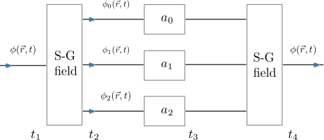
Figure 1: Stern-Gerlach schematic showing the evolution described by Eqs. 1 - 4.

The process just described is unitary, and it comprises the premeasurement stage of the full measurement process. The resulting entangled spin/ancilla system is the system of interest for us - we will describe measurements aimed at exploring its joint properties. But first, as a preliminary, let us define the quantum pointer.

By the time $t_{3}$, the ancilla system has evolved from its excitation vacuum state, $|000\rangle_{a}$ ($N=0$), to single-excitation states ($N=1$), as shown in Table I. Further operations, including all transformations and measurements to be performed on the spin/ancilla system, will preserve the ancilla system in this $N=1$ subspace. This subspace defines the pointer: The pointer is the effective qutrit whose Hilbert space ${\cal H}_{p}$ is spanned by the single-excitation states. We will call these states $|k\rangle_{p}$ ($k=0,1,2$, and $p$ for pointer), and in this notation, Eq. 4 (dropping the common spatial factor) becomes

$$|\Psi\rangle=\frac{1}{\sqrt{3}}\bigg{(}|0\rangle_{s}|0\rangle_{p}+|1\rangle_{s}|1\rangle_{p}+|2\rangle_{s}|2\rangle_{p}\bigg{)},$$ (5)

which indicates a generalized Bell state of the spin-pointer system. Henceforth $|\Psi\rangle$, without the temporal argument, is understood as the state of the spin/pointer system, as prepared at the time $t_{4}$.

Clearly this state generalizes to a spin of arbitrary dimension $d$, and a system of $d$ qubits (dimension $2^{d}$), whose pointer subspace shares the dimension $d$ with the spin. Generalizing Eqs. 4 and 5 (respectively) we have

$$|\Psi\rangle=\frac{1}{\sqrt{d}}\sum_{k=0}^{d-1}|k\rangle_{s}~{}x_{k}|0,...,0\rangle_{a}=\frac{1}{\sqrt{d}}\sum_{k=0}^{d-1}|k\rangle_{s}|k\rangle_{p},$$ (6)

where $x_{k}$ (a Pauli matrix) flips the spin of the $k$th qubit, generating the pointer state $|k\rangle_{p}$.

Table 1: Basis states of the ancilla system with three qubits. The pointer Hilbert space is spanned by the three singly-excited basis states shown. Other states are dynamically excluded.

N	subspace bases	interpretation
0	$|000\rangle$	initialized state
1	$|100\rangle,~{}|010\rangle,~{}|001\rangle$	basis of pointer
2	$|110\rangle,~{}|101\rangle,~{}|011\rangle$	excluded
3	$|111\rangle$	excluded

The restriction to the pointer subspace is enforced by the unitary dynamics of the premeasurement Stern-Gerlach evolution, and it gives rise to the singleness property - the fact that the measurement process will produce a single, unambiguous outcome for an observer or a recording device. There is an observable, $N$, representing the total excitation number of the ancilla system. It is the sum of excitation numbers, $n_{k}=0$ or 1, of the individual qubits $k$ ($k=0,...,d-1$), and it is given by

$$N=\sum_{k=0}^{d-1}n_{k}=\sum_{k=0}^{d-1}\big{(}1+z_{k}\big{)}/2,$$ (7)

where $z_{k}$ is the Pauli $z$-matrix (with eigenvalues $\pm 1$) acting on the $k$th qubit. One can measure $N$ most simply by measuring every individual $z_{k}$ and applying (7). Acting on state (6), the measurement would show that $N=1$, demonstrating the singleness property as listed in Table II. This dramatic correlation within the ancilla system extends to the spin qudit, whose readout (a state index $k$) corresponds to the output ($k$) of the display pointer. This latter correlation is the projection property - the post-measurement spin state is the state identified by the display pointer. (This is called the “post-measurement state-update rule.”)

We have just described the quantum pointer, as distinct from the display pointer. It is “quantum” in two respects that the display pointer is not: It is reversible, and it can be prepared and detected in a superposition of its basis states. That is, no preferred basis set is imposed on it. We will show an example after introducing the relevant observables in the next section.

Table 2: Eigenvalues and Physical Interpretations

eigenvalue	property	physical interpretation
$N=1$	singleness	one and only one detector will register
$Z_{s}^{{\dagger}}Z_{p}=1$	projection	post-measurement spin $\Leftrightarrow$ which detector
$X_{s}X_{p}=1$	superposition	$|\psi(t_{4})\rangle=$ superposition of collapse scenarios

3 OBSERVABLES of the SPIN/POINTER SYSTEM

In the previous section we introduced observables for individual qubits in the ancilla system - the usual Pauli matrices (denoted by lower case $z_{k}$ and $x_{k}$). Here we require observables for two $d$-dimensional systems - the spin and the quantum pointer. These are the generalized Pauli operators (representable as $d\times d$ matrices) which we denote by upper case: $Z_{s}$ and $X_{s}$ for the spin, and $Z_{p}$ and $X_{p}$ for the quantum pointer. The $Z$ are diagonal in the standard basis:

$$Z=\sum_{k=0}^{d-1}|k\rangle~{}\omega^{k}\langle k|,$$ (8)

where $\omega=\exp(2\pi i/d)$ is the $d$th root of unity. Although $Z$ is not hermitian, we refer to it as an observable because it is unitary, and its exponents $k$ are real numbers ($k=0,1,...,d-1$), which label the eigenstates. [In the case of spin, the $\hat{z}$ component of the physical spin takes the values $S_{z}=-S+k$, where $S=(d-1)/2$.]

The canonical conjugates of $Z$ are defined by

$$X=\sum_{k=0}^{d-1}|k+1\rangle\langle k|,$$ (9)

where the state index $k$ is defined modulo $d$. The eigenbasis of $X$, defined by

$$X|k\rangle_{X}=\omega^{k}|k\rangle_{X},$$ (10)

is the inverse quantum Fourier transform NC of the standard basis; that is,

$$|k\rangle_{X}={\cal F^{{\dagger}}}|k\rangle=\frac{1}{\sqrt{d}}\sum_{k^{\prime}}\omega^{-kk^{\prime}}|k^{\prime}\rangle,$$

$$\hbox{where}\hskip 17.07182pt{\cal F}\equiv\frac{1}{\sqrt{d}}\sum_{k}\sum_{k^{\prime}}|k^{\prime}\rangle~{}\omega^{kk^{\prime}}\langle k|,$$ (11)

and ${\cal F}$ and ${\cal F^{{\dagger}}}$, being symmetric, are complex conjugates.

The correlations of interest are described by tensor product operators; the simplest example is $Z_{s}^{{\dagger}}Z_{p}$, which clearly has Eq. 6 as an eigenstate with eigenvalue unity,

$$Z_{s}^{{\dagger}}Z_{p}|\Psi\rangle=|\Psi\rangle.$$ (12)

So, while measurement outcomes of $Z_{s}$ and $Z_{p}$ are separately random, they are perfectly correlated - Eq. 12 represents the projection property, as is summarized in Table II. We will now show that $X_{s}X_{p}$ obeys a similar equation,

$$X_{s}X_{p}|\Psi\rangle=|\Psi\rangle,$$ (13)

which, together with (12), identifies (6) as a generalized Bell state and expresses the superposition property - namely, that 6 is a superposition of the $d$ distinct collapse scenarios. To prove Eq. 13, one can rewrite (6) in terms of the spin and quantum-pointer $X$ bases ($sX$ and $pX$), whereupon it takes the form

$$|\Psi\rangle=\frac{1}{\sqrt{d}}\sum_{k=0}^{d-1}|-k\rangle_{sX}|k\rangle_{pX},$$ (14)

and Eq. 13 follows immediately. It is instructive to show that (6) is in fact the unique solution of the two eigenvalue equations, (12) and (13).

A comment is in order on the measurement of $X_{s}$ and $X_{p}$: Realizing that the readout devices for both the spin and the pointer record standard basis states, one must apply ${\cal F}$ (Eq. 11) to these qudits in order to take their $X$ eigenstates into the corresponding $Z$ eigenstates prior to readout. [Regarding the spin, one cannot simply rotate the Stern-Gerlach magnets, because Fourier transformation of a qutrit, for example, lies in SU(3) and not in SU(2).]

Now, suppose that one measures $X_{s}$ and finds the spin in the eigenstate $|k\rangle_{sX}$. This measurement projects the pointer into the corresponding eigenstate of $X_{p}$, specifically

$$|-k\rangle_{pX}=\frac{1}{\sqrt{d}}\bigg{(}|100...0\rangle+\omega^{k}|010...0\rangle+\omega^{2k}|001...0\rangle+...+\omega^{(d-1)k}|000...1\rangle\bigg{)}.$$ (15)

This is a generalized $W$ state W state - it is a superposition of all the pointer basis states. Its detection requires the measurements of both $X_{s}$ and $X_{p}$. It is noteworthy that these are separately complementary to $Z_{s}^{{\dagger}}$ and $Z_{p}$, respectively, while the products $X_{s}X_{p}$ and $Z_{s}^{{\dagger}}Z_{p}$ are compatible.

A final note - the foregoing illustrates what it means to “observe a superposition.” Ironically, one does not see a superposition as an ambiguity of outcomes; one sees it as a definite outcome of a complementary measurement. In the above case, the sought-for superposition is an eigenstate of $X_{p}$. A measurement of the spin in the basis $X_{s}$ projects the quantum pointer onto the corresponding eigenstate of $X_{p}$, whose eigenvalue is perfectly correlated with the spin outcome. An $X_{p}$ measurement then confirms the projected quantum pointer state.

Nondestructive Measurements

Up to now, measurements of the observables $N$ and $Z_{s}^{{\dagger}}Z_{p}$ have been constructed from readouts of the individual (local) qubits of the ancilla system, and of the spin qudit. Such local measurements preserve the correlations defining the singleness and projection properties, but they destroy the state in the process. To preserve the state, we must reject local information telling us which qubit is excited, or what the qudit spin value is. In this subsection we show how one could, in principle, measure correlation properties while rejecting such local information.

We will describe nondestructive measurements of the complete set of commuting observables ($N$, $Z_{s}^{{\dagger}}Z_{p}$, and $X_{s}X_{p}$). Since the three are compatible, they can all be measured, in principle, on the same state of the same system. For simplicity in the figures to follow, we shall again specialize to the case of $d=3$, from which the generalization to arbitrary $d$ will be obvious.

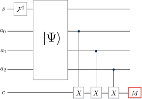
Figure 2: Nondestructive measurement of $N$ on the prepared state $|\Psi\rangle$ (Eq. 5): All five input lines are initialized to 0. The desired spin state (Eq. 1) is prepared by (inverse) Fourier transformation, and then entangled (large box) with the ancilla qubit system via Eqs. 2 - 5. The measurement of $N$ then commences with the $X$ gates, one for each qubit in the ancilla system.

Let us begin with the simplest observable - the ancilla excitation number $N$. Figure 2 shows the prepared state $|\Psi\rangle$ of Eq. (5) (the large box) and an added ancilla qutrit ($c$) to act as a “counter.” Each qubit is coupled to this counter by a controlled-$X$ gate: If a qubit is in the 1 state, then the counter state index ($k$, the exponent in $\omega^{k}$) is advanced by one; if a qubit is in the 0 state, then there is no change. Hence, with the counter index initialized to zero, the readout index will be the total excitation number $N$. For a general input state the outcome would be probabilistic, but in the special case of the prepared state [Eq. (5) or more generally (6)], it will take the value unity with certainty, confirming the singleness property of the pointer.

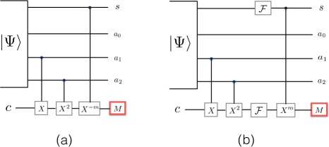
Figure 3: Nondestructive measurements of $Z_{s}^{{\dagger}}Z_{p}$ (a) and $X_{s}X_{p}$ (b) on the same state $|\Psi\rangle$.

Next consider the observable $Z_{s}^{{\dagger}}Z_{p}$, which represents the projection property. Figure 3a is a variation on Fig. 2 in which the controlled-$X$ gates are replaced by the (qubit-dependent) controlled-$X^{l}$ gates, where $l$ is the qubit label ($l=0$, 1, or 2, with 0 being the identity gate). Given the singleness property, these gates impress the pointer state on the counter qutrit ($c$). The spin qutrit is then coupled to ($c$) by a controlled-$X^{-m}$ gate representing $Z_{s}^{{\dagger}}$, where $m$ labels the spin state. Since the prepared state has $m=l$, this last gate cancels the effect of $Z_{p}$, and the readout exponent will be 0, denoting the eigenvalue $Z_{s}^{{\dagger}}Z_{p}\rightarrow 1\equiv\omega^{0}$.

Finally, inclusion of the measurement of $X_{s}X_{p}$ demonstrates the superposition property. Figure 3b builds upon 3a by including the quantum Fourier transforms to take $X$ eigenstates into $Z$ eigenstates. A final controlled-$X^{m}$ gate couples the spin to the counter qutrit ($c$). Since the prepared state has $m=-l$ in the $X_{s}$/$X_{p}$ basis, the readout exponent will again be $M=0$. The upshot of these points is that, if we re-initialize the ancilla qutrit ($c$) after each measurement, it is possible in principle to measure $N$, $Z_{s}^{{\dagger}}Z_{p}$, and $X_{s}X_{p}$ in any order, on the same state of the same system.

This section comprises a generalization of the Ref. JL1 treatment to arbitrary nonbinary spins. It is remarkable that the spin-ancilla system is again described completely by three commuting observables - two for collapse properties and one for the superposition property. Perhaps most remarkable is the emergence of the quantum pointer through the singleness property - a collapse property resulting from the unitary evolution that entangles the spin and the quantum pointer.

4 CHOICES of the POINTER BASIS

The previous section shows how the ancilla system provides a choice of pointer basis - the basis whose elements are identified with the output of the display pointer. Examples discussed were the eigenbases of $Z_{p}$ and $X_{p}$. We note here that there is a continuum of such choices, similarly accessible to experiment.

Consider an arbitrary unitary transformation of the standard pointer basis, $U_{p}|k\rangle_{p}$. There is a corresponding unitary transformation of the spin basis, $V_{s}|k\rangle_{s}$, which leaves the entangled state (6) unchanged: It is straitforward to show that $V$ is the complex conjugate of $U$:

$$V_{s}=U_{s}^{*}\hskip 28.45274pt\Leftrightarrow\hskip 28.45274ptV_{s}U_{p}|\Psi\rangle=|\Psi\rangle,$$ (16)

These transformed bases are eigenbases of the observables

$$O_{p}=U_{p}Z_{p}U_{p}^{{\dagger}}\hskip 22.76228pt\hbox{and}\hskip 22.76228pt\tilde{O}_{s}=V_{s}Z_{s}V_{s}^{{\dagger}},$$ (17)

defined respectively in the quantum pointer and spin Hilbert spaces. We can rewrite (6) in the $\tilde{O}$ - $O$ bases (denoted by subscripts) as

$$|\Psi\rangle=\frac{1}{\sqrt{d}}\sum_{k=0}^{d-1}|k\rangle_{s\tilde{O}}|k\rangle_{pO},$$ (18)

Clearly, this is an eigenstate of $\tilde{O}_{s}^{{\dagger}}O_{p}$, which one could verify experimentally, in principle, by measuring the $\tilde{O}_{s}$ component of the spin downstream, thus projecting the quantum pointer into the corresponding eigenstate of $O_{p}$. To measure these observables, according to the discussion following Eq. 14, one would apply $V_{s}^{{\dagger}}$ to the spin and $U_{p}^{{\dagger}}$ to the quantum pointer prior to the readouts. Incidentally, it is an instructive exercise to recover the Fourier transformed representation (Eq. 14) from this prescription (see the Appendix if interested).

4.1 Coherence Requirement

The necessary condition for basis flexibility and the observation of the superposition property (eg., $\tilde{O}_{s}O_{p}=1$), within the Stern-Gerlach scenario, is that the spatial wave packets must be controlled with sufficient precision to approximate the ideal coherent superposition indicated by Eq. 4 [and understood in (5)]. The challenge has been emphasized by Scully et al.  through the metaphor of Humpty-Dumpty Scully . The challenge has been met - a coherent Stern-Gerlach interferometer has been achieved, but only recently and only for the case of spin-1/2 SG.interf.19 . So, instead of atomic spins, one might consider alternative platforms, such as photons in a Mach-Zender interferometer. Encouraging recent experimental achievements include the entanglement of a photonic qubit with two photonic qutrits Malik (qutrits made with photon orbital angular momentum), and the demonstration of a three-qutrit GHZ state with superconducting transmon circuits Alba .

It is important to emphasize that the coherence requirement for the superposition property does not apply to collapse properties - neither the projection property ($Z_{s}^{{\dagger}}Z_{p}=1$) nor the singleness property ($N=1$). To show why this is the case, consider the worst-case scenario in which there is no coherence between the different wave packets when they are brought back to the same vicinity at the time $t_{4}$. The state of the spin/ancilla system is then described by the density matrix,

$$\rho=\frac{1}{3}\bigg{(}|0\rangle_{s}|0\rangle_{p}\langle 0|_{p}\langle 0|_{s}+|1\rangle_{s}|1\rangle_{p}\langle 1|_{p}\langle 1|_{s}+|2\rangle_{s}|2\rangle_{p}\langle 2|_{p}\langle 2|_{s}\bigg{)},$$ (19)

which would replace Eq. (5). Clearly the average measured value of $X_{s}X_{p}$ vanishes, Tr($\rho X_{s}X_{p}\big{)}=0$, indicating a uniform probability distribution over all possible values, $\omega^{k}$ ($k=0,1,...,d-1$), making it impossible to observe a superposition. On the other hand, every term in (19), and hence $\rho$ itself, is an eigenstate of both $N$ and $Z_{s}^{{\dagger}}Z_{p}$ with eigenvalue unity, indicating definite outcomes for both, Tr($\rho Z_{s}^{{\dagger}}Z_{p}\big{)}=Tr\big{(}\rho N\big{)}=1$. In the case of partial coherence, where nonzero off-diagonal terms such as $|0\rangle_{s}|0\rangle_{p}\langle 1|_{p}\langle 1|_{s}$ contribute to $\rho$, then $X_{s}X_{p}$ will be biased but still random, while $Z_{s}^{{\dagger}}Z_{p}$ and $N$ retain their definiteness.

From the perspective of decoherence theory, the density matrix is derived by tracing over the imperfectly-controlled spatial degrees of freedom, which are playing the role of the environment. It is not the usual active environment responding to the system, but rather a lack of precision in the magnetic field configuration and the resulting failure to reverse the separation of paths. Nevertheless, it selects the preferred basis associated with “which path” information, recorded by the display pointer as the eigenvalue of $Z_{p}$. The reason why $Z_{p}$ is the “default” observable when we lose the flexibility to transform the pointer basis is explained in detail below.

4.2 The Default Basis

As we said in Sec. III, the $k$th readout device is tuned to record an eigenstate of the observable $z_{k}$ of the $k$th qubit. This observable is the (dimensionless) energy of the atom-induced transition $0\rightarrow 1$. The choice to measure $z_{k}$ is made by designing the qubit-readout interaction to depend on this energy. Since the readout is an irreversible decohering process, this interaction selects $z_{k}$ as the preferred basis of an individual qubit. But this is not yet the preferred basis of the pointer. The pointer emerges from the array of all such qubits, each interacting locally with its own readout device. Thus there are $2^{d}$ conceivable readout patterns, but because of the singleness property, only $d$ of these patterns can be realized. These represent just the singly-excited states of the ancilla system, which are the eigenstates of $Z_{p}$, so that $Z_{p}$ is the “observable of the apparatus.” In summary, the qubit-readout interaction determines the preferred basis of individual qubits ($z_{k}$), while the singleness property constrains the array to display eigenstates of $Z_{p}$.

The role of the environment in this determination is restricted to the workings of individual readout devices. It prevents the appearance of superpositions of readings, allowing only a definite 0 or a definite 1. But it does not assign the physical measings ($z_{k}$) to these outcomes.

5 POINTER without ANCILLAE

To identify the quantum pointer in an ordinary apparatus (unaided by ancillae), consider a Stern-Gerlach setup as in Fig. 1, but with a particle detector in place of each ancilla/readout combination. Clearly the detector array forms only the display pointer. So what is the quantum pointer which complements this detector array? That is, what is it that entangles with the object of study?

We answer this question by removing the ancilla ket from Eq. 2. This leaves an expression identical in form to Eq. 5, and we rewrite it as

$$|\Psi(t)\rangle= \frac{1}{\sqrt{3}}\bigg{(}|0\rangle_{s}|\phi_{0}(\vec{r},t)\rangle+|1\rangle_{s}|\phi_{1}(\vec{r},t)\rangle+|2\rangle_{s}|\phi_{2}(\vec{r},t)\rangle\bigg{)}$$ (20)

$$\equiv\frac{1}{\sqrt{3}}\bigg{(}|0\rangle_{s}|0,t\rangle_{p}+|1\rangle_{s}|1,t\rangle_{p}+|2\rangle_{s}|2,t\rangle_{p}\bigg{)},$$ (21)

to show the entanglement between the spin and spatial parts of the atomic state, where the kets $|k,t\rangle_{p}$ in the second line are shorthand for the time dependent wave packets generated by the Schrödinger equation for each spin component $k$. These provide valid pointer states during the time interval ($t_{2}<t<t_{d}$) - that is, after they have become orthogonal but not yet arrived at a detector. Given the singleness property, they are the “which path” states - meaning that if the atom is present on the $k$th path, then it is absent from all the others. We define these states to include the “which path” degree of freedom but not the displacement along the path, so that the quantum pointer is a $d$ dimensional system, coming into existence at $t_{2}$ and disappearing at $t_{d}.$

The observable of the apparatus is the “which path” observable $Z_{p}$ whose eigenvalues ($\omega^{k}$) represent the path. We can define this and other observables formally and prove the desired properties by starting with projection operators analogous to those of JL1 :

$${\cal P}_{k}=\int_{V(k)}d^{3}\vec{r}~{}|\phi_{k}(\vec{r},t)\rangle\langle\phi_{k}(\vec{r},t)|$$ (22)

projects onto that subvolume of the $k$th path which could be occupied during the time interval $t_{2}<t<t_{d}$. The path occupation number $N$ and the pointer observable $Z_{p}$, analogous to Eqs. (7) and (8) in Sec. III, are then

$$N=\sum_{k=0}^{d-1}{\cal P}_{k}$$ (23)

$$\hbox{and}\hskip 28.45274ptZ_{p}=\sum_{k=0}^{d-1}\omega^{k}{\cal P}_{k}.$$ (24)

The state (21) is an eigenstate of $N$ with eigenvalue unity (the singleness property), and of $Z_{s}^{{\dagger}}Z_{p}$ with the same eigenvalue (the projection property). So the local measurements of $Z_{p}$ and $Z_{s}$ are random but perfectly correlated. The state (21) is also an eigenstate of $X_{s}X_{p}$ - a superposition of all possible collapse scenarios, but it is beyond present technology to implement $X_{p}$, since this would require a coherent reconfiguration of paths prior to the detection stage.

Finally, each detector ($k$) serves as the readout device for the corresponding path ($k$), reading (1,0) for (atom, no atom) on that path. This reading is the eigenvalue of ${\cal P}_{k}$. We do not have to engineer an interaction in this case - we only have to coordinate each detector with a path.

An Exception

An instructive example of a measurement without a quantum pointer was pointed out to me by W. K. Wootters. Recall first that a photon polarization measurement is analogous to an atomic spin measurement; the role of the Stern-Gerlach magnetic field is played by a polarizing beam splitter (PBS), which entangles the photon’s polarization with its path. Now consider an unpolarized photon (a completely mixed polarization state), and replace the PBS with an ordinary (non-polarizing) beam splitter. We are now measuring just the photon’s path. What was previously the quantum pointer has now become the measured system, so a separate pointer is superfluous. Note incidentally that the second link in the von Neumann chain is absent; an entangled premeasurement state is not formed, and the path states comprise the preferred basis by default.

6 CONCLUSIONS

We concluded the introduction by asking three questions. This summary reviews the answers.

The first major point developed in this paper is that the pointer is a physical system consisting of two distinct parts, so that it can bridge the gap between the object of study and an observer (conscious or otherwise). The “quantum” part entangles with this object in premeasurement, and then the “display” part reads the quantum part and records the result. This division of labor is necessary because the display part is an effectively classical system - it is entangled with the environment at all times, so that it cannot form a pure entangled state with the object as conventionally assumed in the von Neumann formalism. In our first example, the ancilla qubits form the quantum part, while the display part consists of the respective readout devices. We later showed that this model maps onto a more realistic (unaided) system, in which particle detectors replace the readout devices as the display part, while the path system guiding the atom forms the quantum part.

The second major point is that unitary quantum theory dictates the two “collapse-like” properties: (i) the singleness of outcomes, and (ii) the projection property (the post-measurement state update rule), as well as the more obviously quantum property, (iii) the superposition property, all characterized in Table 2. All of these are observables of the joint object/quantum-pointer system (in its $d^{2}$-dimensional Hilbert space), and as such they are quantum properties. The three comprise a complete set of commuting observables for this system; their three eigenvalues define the entangled state of the joint system completely. The superposition property could be observed, in principle, for this object/quantum-pointer system, although it cannot apply to the display pointer, which behaves classically.

The third major point is that, while decoherence is necessary in preventing the appearance of superpositions of outcomes, it is not sufficient for determining the preferred basis of the pointer. We showed that the pointer emerges from an apparatus utilizing $d$ separate binary detectors, one for each possible output. Decoherence restricts the output of each detector to a definite 1 or 0, thus imposing classical behavior. However, the assignment of meaning to the possible outputs (providing the post-measurement state updates) must be provided by the interaction (or simply the coordination) between the quantum and display parts of the pointer, as is spelled out in Subsec. 4.2.

Let us briefly summarize the implications for foundations: First, the naive concept of a single apparatus that can behave either quantum mechanically or classically is unrealistic. Secondly, the singleness of outcomes, and the projection property, are quantum properties of the entangled premeasurement state. And finally, it is the observer, through the arrangement of the apparatus, who determines the preferred basis of the pointer. The last point may be the most unconventional of the three, at variance with the orthodox theory Brasil ; Zurek.81 ; Schloss.04 . But it depends critically on the first point - the division of the pointer into quantum and classical parts.

Acknowledgements

It is a pleasure to thank Bill Wootters and Brian Odom for enlightening conversations on the subject of this paper.

Appendix: Recovery of simultaneous Fourier transforms

Here we show that the simultaneous Fourier transform description of the entangled state (6) [based on Eqs. (10) - 11)] is recovered from the general prescription given in Sec. IV. The Fourier transformed basis, $|k\rangle_{pX}={\cal F}^{{\dagger}}|k\rangle_{p}$, corresponds to

$$O_{p}\rightarrow X_{p}={\cal F}^{{\dagger}}Z_{p}{\cal F},$$ (25)

so that the general unitary transformations defined in Eqs. 16 and 17 are specialized to

$$U_{p}={\cal F}^{{\dagger}}\hskip 42.67912pt\hbox{and}\hskip 42.67912ptV_{s}=U_{s}^{*}={\cal F}.$$ (26)

since complex conjugation amounts to inversion of the Fourier transformation. And since this inversion amounts to a sign change of labels, the entangled state (6) is rewritten as (14). The prescription of Sec. V tells us that this state is an eigenstate of $\tilde{O}_{s}^{{\dagger}}O_{p}$, and that

$$\tilde{O}_{s}=V_{s}Z_{s}V_{s}^{{\dagger}}={\cal F}Z_{s}{\cal F}^{{\dagger}}=X^{{\dagger}}$$ (27)

so that

$$\tilde{O}_{s}^{{\dagger}}O_{p}=X_{s}X_{p},$$ (28)

as is needed for consistency with Eq. 13. This shows that the Fourier transformed representation of Sec. III is recovered by the general prescription of Sec. IV.

References

- (1) J. von Neumann, Mathematical Foundations of Quantum Mechanics, trans. R. T. Beyer (Princeton University Press, Princeton, 1955), pp.437-445.
- (2) C. A. Brasil and L. A. de Castro, Understanding the pointer states, Eur. J. Phys. 36, 065024 (2015).
- (3) F. London and E. Bauer, The Theory of Observation in Quantum Mechanics, in Quantum Theory and Measurement, (Eds.) J. A. Wheeler and W. H. Zurek, pp. 217-259 (Princeton University Press, 1983).
- (4) E. P. Wigner, Remarks on the Mind-Body Question, in The Scientist Speculates, (Ed.) I J. Good (Heinemann, London, 1961).
- (5) H. Everett, Relative State Formulation of Quantum Mechanics, Rev. Mod. Phys. 29, 454 (1957).
- (6) B. S. DeWitt and N. Graham, The Many-Worlds Interpretation of Quantum Mechanics, (Princeton University Press, Princeton, 1973).
- (7) M. Jammer, The philosophy of quantum mechanics: the interpretations of quantum mechanics in historical perspective (Wiley, New York, 1974).
- (8) L. A. de Castro, O. P. de Sá Neto and C. A. Brasil, An introduction to quantum measurements with an historical motivation, Acta Physica Slovaca 69, 1 (2019).
- (9) S. Weinberg, Lectures on Quantum Mechanics, (Cambridge Univ. Press, 2013).
- (10) H. D. Zeh, On the interpretation of measurement in quantum theory, Foundations of Physics 1, 69 (1970).
- (11) W. H. Zurek, Pointer basis of quantum apparatus: Into what mixture does the wave packet collapse? Phys. Rev. D 24, 1516 (1981).
- (12) W. H. Zurek, Environment-induced superselection rules, Phys. Rev. D 26, 1862 (1982).
- (13) E. Joos and H. D. Zeh, The emergence of classical properties through interaction with the environment, Zeit. Phys. B: Condensed Matter 59, 223 (1985).
- (14) W. H. Zurek, Decoherence, einselection, and the quantum origins of the classical,’Rev. Mod. Phys. 75, 715 (2003), also see Physics Today 44, 36 (1991).
- (15) M. Schlosshauer, Decoherence, the measurement problem, and interpretations of quantum mechanics, Rev. Mod. Phys. 76, 1267 (2005).
- (16) E. Joos et. al., Decoherence and the Appearance of a Classical World in Quantum Theory, (Springer, 2003).
- (17) M. Schlosshauer, The quantum-to-classical transition and decoherence, in Handbook of Quantum Information, M. Aspelmeyer, T. Calarco, J. Eisern, and F. Schmidt-Kaler (Eds.), (Springer: Berlin, Heidelberg, 2014).
- (18) J. Lawrence, Observing a quantum measurement, Found. Phys. 52, 14 (2022).
- (19) M. A. Nielsen and I. L. Chuang, Quantum Computation and Quantum Information, (Cambridge University Press, Cambridge, 2000), p. 217.
- (20) W. Dür, G. Vidal, and J. I. Cirac, Three qubits can be entangled in two inequivalent ways, Phys. Rev. A 62, 062314 (2000).
- (21) M. O. Scully, B.-G. Englert, and J. Schwinger, Is spin coherence like Humpty-Dumpty? I. Simplified treatment, Found. Phys. 18, 1045 (1988).
- (22) Y. Margalit, Z. Zhou, S. Machluf, Y. Japha, S. Moukouri, and R. Folman, Analysis of a high-stability Stern-Gerlach spatial fringe interferometer, New J. Phys. 21, 073040 (2019).
- (23) M. Malik, M. Erhard, M. Huber, M. Krenn, R. Fickler, and A. Zeilinger, Multi-photon entanglement in high dimensions, Nature Photonics 10, 248 (2016).
- (24) A. Cervera-Lierta, M. Krenn, A. Aspuru-Guzik, and A. Galda, Experimental high-dimensional Greenberger-Horne-Zeilinger entanglement with superconducting transmon qutrits, Phys. Rev. Applied 17, 024062 (2022).