Scattering of spin waves by a Bloch domain wall: effect of the dipolar interaction

Abstract

It is known that a Bloch domain wall in an anisotropic ferromagnet is transparent to spin waves. This result is derived by approximating the dipolar interaction between magnetic moments by an effective anisotropy interaction. In this paper we study the the scattering of spin waves by a domain wall taking into account the full complexity of the dipolar interaction, treating it perturbatively in the distorted wave Born approximation. Due to the peculiarities of the dipolar interaction, the implementation of this approximation is not straightforward. The difficulties are circumvented here by realizing that the contribution of the dipolar interaction to the spin wave operator can be split into two terms: i) an operator that commutes with the spin wave operator in absence of dipolar interaction, and ii) a local operator suitable to be treated as a perturbation in the distorted wave Born approximaton. We analyze the scattering parameters obtained within this approach. It turns out that the reflection coefficient does not vanish in general, and that the transmitted waves suffer a lateral shift even at normal incidence. This lateral shift can be greatlty enhanced by making the spin wave go through an array of well separated domain walls. The outgoing spin wave will no be attenuated by the scattering at the domain walls since the reflection coefficient vanishes at normal incidence. This effect may be very useful to control the spin waves in magnonic devices.

I Introduction

Replacing electric currents by spin waves as a means to transfer and manipulating information in information technology devices is currently seen as an alternative that might be revolutionary, due to the ultralow power consumption involved in the propagation of spin waves, in comparison with electric currents, which dissipate energy through ohmic losses. This fact, besides its intrinsic interest from the fundamental physics point of view, makes magnonics a very active field of research nowadays Pirro2021 ; Barman2021 ; Yu2021 ; Chumak2015 . Indeed, several kinds of logical devices based on spin waves have been proposed, as magnonic logic gates Schneider2008 , magnonic logic circuits Khitun2010 , and a magnon transistor Chumak2014 .

To develop a technology based partly in spin waves it is necessary to have materials with adequate magnetic properties, especially in what concerns the attenuation of spin waves. Ultralow magnetic damping is shown by some insulators, notably the yttrium iron garnet Yu2014 ; Hauser2016 , and has also been recently reported in thin films of a family of Heusler half-metals Guillemard2019 . It is also necessary to have means to control and manipulate spin waves. This can be achieved in part by controlling the magnetic textures on which spin waves propagate, either by manipulating them externally, producing graded magnetic textures Davies2015a ; Davies2015b ; Dzyapko2016 ; Vogel2015 ; Vogel2018 , or by exploiting the inhomogeneous magnetic states characteristic of chiral magnets, as skyrmion and one dimensional chiral soliton lattices. These states have the advantage of appearing spontaneously and being controllable by external means like temperature or magnetic field Bogdanov1994a ; Muhlbauer2009 ; Yu2010 ; Laliena2017b ; Laliena2018c ; Togawa2012 ; Laliena2016b ; Laliena2017a .

One tool to control the spin waves is the scattering (reflection and transmission) at artificially created interfaces, or at artificial magnetic patterns. This scattering induces interesting effects like Goos-Hänchen displacements Dadoenkova2012 ; Gruszecki2014 ; Gruszecki2017 ; Mailyan2017 ; Stigloher2018 ; Wang2019 ; Zhen2020 , the Hartman effect Klos2018 and the Talbot effect Golebiewski2020 , which could be used to manipulate the spin wave.

Spin waves are also scattered by magnetic solitons like domain walls Braun1994 , skyrmions Schutte2014 or one dimensional chiral solitons Laliena2021 , producing effects that could also be useful to control the spin waves. For instance, the scattering by a one dimensional soliton causes a lateral shift of the propagation direction of the scattered waves analogous to the Goos-Hänchen displacement Laliena2021 . It has been proposed that the scattering by domain walls can be used for spin wave interferometry Hertel2004 or as a spin wave valve Hamalainen2018 . The scattering by solitons has the additional advantage that these kind of magnetic structures can be moved across the material under the action of external influences like magnetic fields or electric currents Schryer1974 ; Thiaville2005 ; Woo2016 ; Laliena2020 ; Osorio2021 .

In this paper we study the scattering of spin waves by a Bloch domain wall in an anisotropic ferromangnet. It is known that such a domain wall is transparent to the spin waves since the reflection coefficient does vanish. This result is based on theoretical computations that either ignore the dipolar interaction or approximate it by an effective local anisotropy Braun1994 ; Winter1961 ; Thiele1973 . Here we show that the domain wall does actually reflect the spin waves if the dipolar interaction is properly taken into account. We obtain the reflected and transmitted amplitudes treating the dipolar interaction as a perturbation and using the distorted wave Born approximation. Due to the nature of the dipolar interaction this approximation is not straightforward, and it is necessary to split the spin wave operator into an operator that can be included in the “unperturbed” operator plus another localized operator, suitable to be treated in the Born approximation. The reflection coefficient thus obtained is non zero, but it vanishes for normal incidence, what agrees with the numerical simulations of Hertel et al. Hertel2004 , which take into account properly the dipolar interaction.

II The domain wall of an anisotropic ferromagnet

Let us consider a ferromagnet with uniaxial anisotropy of easy-axis type at a temperature sufficiently low, so that the fluctuations of the modulus of the magnetization, $M_{s}$, can be neglected. Then its magnetization is characterized by a unit vector field ${\boldsymbol{n}}$. We use a cartesian coordinate system with axes given by the three orthonormal vectors ${\boldsymbol{x}}$, ${\boldsymbol{y}}$ and ${\boldsymbol{z}}$ and coordinates $x$, $y$ and $z$ along these axes. The points of space are represented by vectors like $\boldsymbol{r}$, with $x={\boldsymbol{x}}\dotproduct\boldsymbol{r}$, etc., and $r=|\boldsymbol{r}|$. We will also use sometimes the notation $x_{1}=x$, $x_{2}=y$, and $x_{3}=z$, and ${\boldsymbol{x}}_{1}={\boldsymbol{x}}$, ${\boldsymbol{x}}_{2}={\boldsymbol{y}}$ and ${\boldsymbol{x}}_{3}={\boldsymbol{z}}$, and then $x_{i}={\boldsymbol{x}}_{i}\dotproduct\boldsymbol{r}$. The magnet is oriented so that its anisotropy axis coincides with ${\boldsymbol{z}}$. The dynamics of the magnetization is derived from the energy functional $\mathcal{E}=\int d^{3}rw(\boldsymbol{r})$ with

$$w(\boldsymbol{r})=A\sum_{i=1}^{3}(\partial_{x_{i}}{\boldsymbol{n}})^{2}-K_{u}({\boldsymbol{z}}\dotproduct{\boldsymbol{n}})^{2}-\frac{\mu_{0}M_{s}^{2}}{2}\,{\boldsymbol{n}}\dotproduct\boldsymbol{h}_{d},$$ (1)

where the succesive terms in $w(\boldsymbol{r})$ correspond to the ferromagnetic exchange interaction, the anisotropy interaction, and the dipolar interaction. The constants $A>0$ and $K_{u}>0$ represent the strengths of the exchange and anisotropy interaction, respectively, and $\mu_{0}$ is the vacuum permeability. The vector field $\boldsymbol{h}_{d}$ is the dimensionless magnetostatic field, which is the solution of the boundary value problem

$$\nabla\crossproduct\boldsymbol{h}_{d}=0,\quad\nabla\dotproduct\boldsymbol{h}_{d}=-\nabla\dotproduct{\boldsymbol{n}},$$ (2)

in the whole space (interior and exterior to the magnet), with $\boldsymbol{h}_{d}$ decaying sufficiently fast as $r\to\infty$ as a condition.

The dynamics of the magnetization obeys the Landau-Lifschitz-Gilbert equation,

$$\partial_{t}{\boldsymbol{n}}=\gamma\boldsymbol{B}_{\mathrm{eff}}\crossproduct{\boldsymbol{n}}+\alpha{\boldsymbol{n}}\crossproduct\partial_{t}{\boldsymbol{n}},$$ (3)

where $\gamma$ is the electron gyromagnetic factor, $\alpha$ is the Gilbert damping constant, and $\boldsymbol{B}_{\mathrm{eff}}$ is the effective field, given by the variational derivative (the first variation) of the energy functional: $\boldsymbol{B}_{\mathrm{eff}}=-(1/M_{s})\delta\mathcal{E}/\delta{\boldsymbol{n}}$. In the present case it is

$$\boldsymbol{B}_{\mathrm{eff}}=\frac{2A}{M_{s}}\Big{(}\nabla^{2}{\boldsymbol{n}}+q_{0}^{2}({\boldsymbol{z}}\dotproduct{\boldsymbol{n}}){\boldsymbol{z}}+\epsilon q_{0}^{2}\,\boldsymbol{h}_{d}\Big{)},$$ (4)

where $q_{0}=\sqrt{K_{u}/A}$ has the dimensions of inverse length and $\epsilon=\mu_{0}M_{s}^{2}/2K_{u}$ is dimensionless. Notice that at a fixed time $\boldsymbol{h}_{d}$ is a linear functional of ${\boldsymbol{n}}$, given by the solution of (2). Since we are interested in the scattering of spin waves, we neglect the damping term, assuming that the spin waves are able to propagate to long enough distances without appreciable attenuation.

Let us consider a large magnet, which eventually will be infinite. Let $L_{x}$, $L_{y}$, and $L_{z}$ be the system dimensions along the ${\boldsymbol{x}}$, ${\boldsymbol{y}}$ and ${\boldsymbol{z}}$ directions, respectively, and let $L_{z}$ be much larger than $L_{x}$ and $L_{y}$. In the limit $L_{z}\to\infty$ the ferromagnetic state with uniform magnetization along the ${\boldsymbol{z}}$ direction is an equilibrium state, since the magnetostatic field inside the magnet vanishes in this limit, and therefore the energy functional attains its absolute minimum. After the $L_{z}\to\infty$ limit we take $L_{x}\to\infty$ and $L_{y}\to\infty$. By symmetry, the uniform state with magnetization pointing along the $-{\boldsymbol{z}}$ direction is another equilibrium state.

This system has domain walls as metastable states. To see this, let us neglect first the dipolar interaction. It is well known that the Euler-Lagrange equations of the functional (1) with the dipolar interaction term removed have the solution

$${\boldsymbol{n}}_{0}(\boldsymbol{r})=\sin\theta(x){\boldsymbol{y}}+\cos\theta(x){\boldsymbol{z}},$$ (5)

where $\theta(x)=2\atan\big(\mathrm{e}^{q_{0}x}\big{missing})$. This state is a domain wall centered at $x=0$, which separates a domain with ${\boldsymbol{n}}(\boldsymbol{r})\to{\boldsymbol{z}}$ for $x\to-\infty$ from the opposite domain, with ${\boldsymbol{n}}_{0}(\boldsymbol{r})\to-{\boldsymbol{z}}$, for $x\to+\infty$. The magnetostatic field produced by the magnetization field (5) vanishes in the infinite system, and therefore (5) is a solution of the Euler-Lagrange equations with dipolar interaction. Moreover, the dipolar energy reaches its minimum (zero) at the domain wall state, which consequently remains as a metastable state when the dipolar interaction is taken into account.

III Spin wave operator in presence of a domain wall

Let us consider perturbations of the domain wall state, which in general can be described by two real fields $\xi_{1}$ and $\xi_{2}$, so that

$${\boldsymbol{n}}=\big{(}1+\xi_{1}^{2}+\xi_{2}^{2}\big{)}^{1/2}{\boldsymbol{n}}_{0}+\xi_{1}{\boldsymbol{e}}_{1}+\xi_{2}{\boldsymbol{e}}_{2},$$ (6)

where $\{{\boldsymbol{e}}_{1},{\boldsymbol{e}}_{2},{\boldsymbol{n}}_{0}\}$ is a right-handed orthonormal triad. Notice that ${\boldsymbol{e}}_{1}$ and ${\boldsymbol{e}}_{2}$ depend on $\boldsymbol{r}$, since ${\boldsymbol{n}}_{0}$ does. We take

$${\boldsymbol{e}}_{1}(\boldsymbol{r})={\boldsymbol{x}},\quad{\boldsymbol{e}}_{2}(\boldsymbol{r})=\cos\theta(x){\boldsymbol{y}}-\sin\theta(x){\boldsymbol{z}}.$$ (7)

We consider local perturbations, $\delta{\boldsymbol{n}}=\xi_{1}{\boldsymbol{e}}_{1}+\xi_{2}{\boldsymbol{e}}_{2}$, whose absolute value decreases to zero rapidly enough as $r\to\infty$. These local perturbations propagate through the magnet as spin waves. Their dynamics are governed by the linearized Landau-Lifschitz-Gilbert equation, which, neglecting the damping term, has the form

$$\partial_{t}\delta{\boldsymbol{n}}=\gamma\boldsymbol{B}_{\mathrm{eff}}^{(0)}\crossproduct\delta{\boldsymbol{n}}+\gamma\delta\boldsymbol{B}_{\mathrm{eff}}\crossproduct{\boldsymbol{n}}_{0},$$ (8)

where $\boldsymbol{B}_{\mathrm{eff}}^{(0)}$ is the effective field corresponding to the metastable state ${\boldsymbol{n}}_{0}$

$$\boldsymbol{B}_{\mathrm{eff}}^{(0)}=\frac{2A}{M_{s}}q_{0}^{2}\cos(2\theta){\boldsymbol{n}}_{0},$$ (9)

and $\delta\boldsymbol{B}_{\mathrm{eff}}$ is the effective field to first order in the perturbation $\delta{\boldsymbol{n}}$,

$$\delta\boldsymbol{B}_{\mathrm{eff}}=\frac{2A}{M_{s}}\Big{(}\nabla^{2}\delta{\boldsymbol{n}}+q_{0}^{2}({\boldsymbol{z}}\dotproduct\delta{\boldsymbol{n}}){\boldsymbol{z}}+\epsilon q_{0}^{2}\,\delta\boldsymbol{h}_{d}\Big{)},$$ (10)

with $\delta\boldsymbol{h}_{d}$ being the magnetostatic field created by the perturbation, which is the solution of

$$\nabla\crossproduct\delta\boldsymbol{h}_{d}=0,\quad\nabla\dotproduct\delta\boldsymbol{h}_{d}=-\nabla\dotproduct\delta{\boldsymbol{n}}.$$ (11)

Projecting equation (8) onto ${\boldsymbol{e}}_{1}$ and ${\boldsymbol{e}}_{2}$ we obtain the equations for the dynamics of $\xi_{1}$ and $\xi_{2}$:

$$\partial_{t}\xi_{1}=-W\xi_{2}+\omega_{0}\,\epsilon\,(\delta\boldsymbol{h}_{d}\crossproduct{\boldsymbol{n}}_{0})\dotproduct{\boldsymbol{e}}_{1},$$ (12)

$$\partial_{t}\xi_{2}=W\xi_{1}+\omega_{0}\,\epsilon\,(\delta\boldsymbol{h}_{d}\crossproduct{\boldsymbol{n}}_{0})\dotproduct{\boldsymbol{e}}_{2},$$ (13)

where $\omega_{0}=2\gamma Aq_{0}^{2}/M_{s}$ and $W$ is the Schrödinger operator

$$W=-\frac{\omega_{0}}{q_{0}^{2}}\nabla^{2}+\omega_{0}-2\omega_{0}\sech^{2}(q_{0}x).$$ (14)

The dipolar field determined by equations (11) is linear in $\xi_{1}$ and $\xi_{2}$ and thus we have

$$\big{[}\delta\boldsymbol{h}_{d}(\boldsymbol{r})\crossproduct{\boldsymbol{n}}_{0}(x)\big{]}\dotproduct{\boldsymbol{e}}_{1}(x)=\big{(}D_{11}\xi_{1}\big{)}(\boldsymbol{r})+\big{(}D_{12}\xi_{2}\big{)}(\boldsymbol{r}),$$ (15)

$$\big{[}\delta\boldsymbol{h}_{d}(\boldsymbol{r})\crossproduct{\boldsymbol{n}}_{0}(x)\big{]}\dotproduct{\boldsymbol{e}}_{2}(x)=\big{(}D_{21}\xi_{1}\big{)}(\boldsymbol{r})+\big{(}D_{22}\xi_{2}\big{)}(\boldsymbol{r}),$$ (16)

where the $D_{\alpha\beta}$ are linear operators which will be determined in the next section. Thus, defining $\xi$ as the two-component column vector $\xi=(\xi_{1},\xi_{2})^{T}$, the spin wave equation can be written as

$$\partial_{t}\xi=\Omega\xi,$$ (17)

where $\Omega=\Omega_{0}+\epsilon\omega_{0}D$ is a linear operator with

$$\Omega_{0}=\begin{pmatrix}0&-W\\ W&0\end{pmatrix},\quad D=\begin{pmatrix}D_{11}&D_{12}\\ D_{21}&D_{22}\end{pmatrix}.$$ (18)

If the dipolar interaction is neglected, or if it is approximated by an effective interaction included in $K_{u}$, the dynamics of the spin waves is given by $\Omega_{0}$. This operator has been studied since long ago by a number of researchers (see references Winter1961, ; Thiele1973, ; Braun1994, ; Hertel2004, ; Bayer2005, ; Kishine2011, ; Borys2016, ; Whitehead2017, ). Let us recall its spectral properties, which are needed in the following. Let $\psi$ be an eigenfunction of $W$, with eigenvalue $\nu\geq 0$ (since the spectrum of $W$ is non negative), so that $W\psi=\nu\psi$. Then the two states

$$\frac{1}{\sqrt{2}}\begin{pmatrix}1\\ -\mathrm{i}\end{pmatrix}\psi,\quad\frac{1}{\sqrt{2}}\begin{pmatrix}1\\ \mathrm{i}\end{pmatrix}\psi,$$ (19)

are eigenstates of $\Omega_{0}$ with eigenvalues $+\mathrm{i}\nu$ and $-\mathrm{i}\nu$, respectively. Hence, the spectral properties of $\Omega_{0}$ are fully determined by those of $W$.

To obtain the spectrum of $W$ we perform a Fourier transform in the variables $y$ and $z$,

$$\tilde{\psi}(x,\boldsymbol{k}_{p})=\int d^{2}r_{p}\mathrm{e}^{-\mathrm{i}\boldsymbol{k}_{p}\dotproduct\boldsymbol{r}_{p}}\psi(x,\boldsymbol{r}_{p}),$$ (20)

where $\boldsymbol{k}_{p}=k_{y}{\boldsymbol{y}}+k_{z}{\boldsymbol{z}}$ and $\boldsymbol{r}_{p}=y{\boldsymbol{y}}+z{\boldsymbol{z}}$, and the spectral equation for $W$ becomes

$$\frac{\omega_{0}}{q_{0}^{2}}\Big{(}-\frac{d^{2}}{dx^{2}}+k_{p}^{2}+q_{0}^{2}-2q_{0}^{2}\sech^{2}(q_{0}x)\Big{)}\tilde{\psi}(x,\boldsymbol{k}_{p})=\nu\,\tilde{\psi}(x,\boldsymbol{k}_{p}).$$ (21)

This is a one dimensional time independent Schrödinger equation with potential $-2q_{0}^{2}\sech^{2}(q_{0}x)$, which is exactly solvable Drazin1989 . Its spectrum consists of one bound state with eigenvalue $\nu_{B}=\omega_{0}k_{p}^{2}/q_{0}^{2}$ and eigenfunction

$$\phi_{B}(x)=\frac{q_{0}}{\sqrt{2}}\sech(q_{0}x),$$ (22)

and a continuum spectrum above a gap, given by $\omega_{G}=\nu_{B}+\omega_{0}$. The continuum spectrum is parametrized by a real number (wave number) $k_{x}$ as

$$\nu(\boldsymbol{k})=\omega_{0}\frac{k_{x}^{2}}{q_{0}^{2}}+\omega_{G},$$ (23)

with $\boldsymbol{k}=k_{x}{\boldsymbol{x}}+\boldsymbol{k}_{p}$, and has the eigenfunctions

$$\phi_{k_{x}}(x)=\frac{1}{\sqrt{q_{0}^{2}+k_{x}^{2}}}\mathrm{e}^{\mathrm{i}k_{x}x}\big{(}q_{0}\tanh(q_{0}x)-\mathrm{i}k_{x}\big{)}.$$ (24)

The eigenfunctions satisfy the normalization condition

$$\int_{-\infty}^{\infty}\phi_{B}^{2}(x)dx=1,$$ (25)

$$\int_{-\infty}^{\infty}\phi_{k_{x}}(x)^{*}\phi_{k_{x}^{\prime}}(x)dx=\delta(k_{x}-k_{x}^{\prime}),$$ (26)

and the closure relation

$$\phi_{B}(x)\phi_{B}(x^{\prime})+\int_{-\infty}^{\infty}\frac{dk_{x}}{2\pi}\phi_{k_{x}}(x)\phi_{k_{x}}^{*}(x^{\prime})=\delta(x-x^{\prime}).$$ (27)

The eigenstates of $\Omega_{0}$ are obtained by substituting $\psi$ in (19) by $\mathrm{e}^{\mathrm{i}\boldsymbol{k}_{p}\dotproduct\boldsymbol{r}_{p}}\phi_{B}(x)$ or by $\mathrm{e}^{\mathrm{i}\boldsymbol{k}_{p}\dotproduct\boldsymbol{r}_{p}}\phi_{k_{x}}(x)$. The closure relation (27) ensures that $\Omega_{0}$ has the spectral representation

$$\Omega_{0}(\boldsymbol{r},\boldsymbol{r}^{\prime})=\int\frac{d^{2}k_{p}}{(2\pi)^{2}}\mathrm{e}^{\mathrm{i}\boldsymbol{k}_{p}\dotproduct(\boldsymbol{r}_{p}-\boldsymbol{r}_{p}^{\prime})}\tilde{\Omega}_{0}(\boldsymbol{k}_{p},x,x^{\prime}),$$ (28)

where

$$\tilde{\Omega}_{0}(\boldsymbol{k}_{p},x,x^{\prime})=\begin{pmatrix}0&-\nu_{B}\\ \nu_{B}&0\end{pmatrix}\phi_{B}(x)\phi_{B}(x^{\prime})+\int_{-\infty}^{\infty}\frac{dk_{x}}{2\pi}\begin{pmatrix}0&-\nu(\boldsymbol{k})\\ \nu(\boldsymbol{k})&0\end{pmatrix}\phi_{k_{x}}(x)\phi_{k_{x}}^{*}(x^{\prime}).$$ (29)

From now on we will not show explicitely the $\boldsymbol{k}_{p}$ dependence of $\tilde{\Omega}_{0}$, which has to be understood.

The spin wave spectrum contains two states bound to the domain wall, sometimes called Winter modes Winter1961 , whose spatial distribution is described by the wave function $\phi_{B}(x)$, which decays exponentially for $|x|\to\infty$. These modes are very interesting since they only propagate on the domain wall plane, so that they might be used as a wave guide for spin waves GarciaSanchez2015 . Spin wave propagation bound to the domain wall has been experimentally observed by Wagner et al. Wagner2016 .

In this paper, however, we focus on the scattering of unbounded spin waves by the domain wall. For that we will need the asymptotic behavior of $\phi_{k_{x}}(x)$ as $x\to\pm\infty$, which is given by

$$\phi_{k_{x}}(x)\sim-\mathrm{i}\,\mathrm{e}^{\pm\mathrm{i}\delta_{0}}\mathrm{e}^{\mathrm{i}k_{x}x},\quad x\to\pm\infty,$$ (30)

where

$$\delta_{0}=\pi/2-\atan(k_{x}/q_{0}).$$ (31)

It is well known that the $2q_{0}^{2}\sech^{2}(q_{0}x)$ potential is reflectionless Drazin1989 , and this quality is inherited by the $\Omega_{0}$ operator. Therefore the domain wall does not reflect the spin waves if the dipolar interaction is neglected, or if it is approximated by an effective magnetic anisotropy Braun1994 ; Winter1961 ; Thiele1973 .

IV The contribution of the dipolar interaction

Let us analyze the form of the $D$ operator, which gives the contribution of the dipolar interaction to the spin wave operator.

Since we consider local perturbations which vanish sufficiently rapid as $r\to\infty$, the solution of equations (11) is

$$\delta\boldsymbol{h}_{d}(\boldsymbol{r})=-\frac{1}{4\pi}\int d^{3}r^{\prime}\,\frac{\boldsymbol{r}-\boldsymbol{r}^{\prime}}{|\boldsymbol{r}-\boldsymbol{r}^{\prime}|^{3}}\,\nabla\dotproduct\delta{\boldsymbol{n}}(\boldsymbol{r}^{\prime}).$$ (32)

Combining this expression with equations (15) and (16) we obtain the form of the $D$ operator. Noticing that ${\boldsymbol{e}}_{1}$ and ${\boldsymbol{e}}_{2}$ are independent of $y$ and $z$, we perform the Fourier expansion in the variables $y$ and $z$ (recall that $\boldsymbol{r}_{p}=y{\boldsymbol{x}}+z{\boldsymbol{z}}$ and $\boldsymbol{k}_{p}=k_{y}{\boldsymbol{x}}+k_{z}{\boldsymbol{z}}$):

$$\xi_{\alpha}(x,\boldsymbol{r}_{p})=\int\frac{d^{2}k_{p}}{(2\pi)^{2}}\mathrm{e}^{\mathrm{i}\boldsymbol{k}_{p}\dotproduct\boldsymbol{r}_{p}}\tilde{\xi}_{\alpha}(x,\boldsymbol{k}_{p}),\;\;\alpha=1,2.$$ (33)

In this way we get

$$\big{(}D_{\alpha\beta}\xi_{\beta}\big{)}(x,\boldsymbol{r}_{p})=\int\frac{d^{2}k_{p}}{(2\pi)^{2}}\mathrm{e}^{\mathrm{i}\boldsymbol{k}_{p}\dotproduct\boldsymbol{r}_{p}}\big{(}\tilde{D}_{\alpha\beta}\tilde{\xi}_{\beta}\big{)}(x,\boldsymbol{k}_{p}),$$ (34)

where no summation in $\beta$ is is to be understood and

$$\big{(}\tilde{D}_{\alpha\beta}\tilde{\xi}_{1}\big{)}(x,\boldsymbol{k}_{p})=\int_{-\infty}^{\infty}\!\!dx^{\prime}\tilde{D}_{\alpha\beta}(x,x^{\prime},\boldsymbol{k}_{p})\tilde{\xi}_{\beta}(x^{\prime},\boldsymbol{k}_{p}),$$ (35)

where the kernels are given by

$$\tilde{D}_{11}(x,x^{\prime},\boldsymbol{k}_{p}) = -\mathrm{i}F(x,\boldsymbol{k}_{p})\sigma(x-x^{\prime})\rho(x-x^{\prime}),\;\;$$ (36)

$$\tilde{D}_{12}(x,x^{\prime},\boldsymbol{k}_{p}) = -F(x,\boldsymbol{k}_{p})\rho(x-x^{\prime})F(x^{\prime},\boldsymbol{k}_{p})$$ (37)

$$\tilde{D}_{21}(x,x^{\prime},\boldsymbol{k}_{p}) = \delta(x-x^{\prime})-\rho(x-x^{\prime}),$$ (38)

$$\tilde{D}_{22}(x,x^{\prime},\boldsymbol{k}_{p}) = \mathrm{i}\sigma(x-x^{\prime})\rho(x-x^{\prime})F(x^{\prime},\boldsymbol{k}_{p}).$$ (39)

In these expressions we introduce the functions

$$\sigma(x)=x/|x|,\quad\rho(x)=\frac{k_{p}}{2}\mathrm{e}^{-k_{p}|x|}.$$ (40)

and $F(x,\boldsymbol{k}_{p})$, which is the projection of $\boldsymbol{k}_{p}/k_{p}$ onto ${\boldsymbol{e}}_{2}(x)$:

$$F(x,\boldsymbol{k}_{p})=\frac{k_{y}}{k_{p}}\cos\theta(x)-\frac{k_{z}}{k_{p}}\sin\theta(x).$$ (41)

Notice that $F(x,\boldsymbol{k}_{p})\to\mp k_{y}/k_{p}$ as $x\to\pm\infty$. Some details on the derivations of the operators $\tilde{D}_{\alpha\beta}$ are given in appendix A.

For fixed $\boldsymbol{k}_{p}$ the operator $\tilde{D}$ is not invariant under reflection about the domain wall center, $x=0$. This is due to the fact that the the equilibium state ${\boldsymbol{n}}_{0}(x)$ is not invariant under reflection with respect to the ${\boldsymbol{y}}{\boldsymbol{z}}$ plane (not even the ferromagnetic state ${\boldsymbol{n}}_{0}(x)={\boldsymbol{z}}$ is invariant, since ${\boldsymbol{n}}$ is an axial vector). However, ${\boldsymbol{n}}_{0}(x)$ is invariant under the composition of a reflection with respect to ${\boldsymbol{y}}{\boldsymbol{z}}$ plane and a reflection with respect to the ${\boldsymbol{x}}{\boldsymbol{y}}$ plane. This means that $\tilde{D}$ is invariant under the transformation $x\to-x$ and $k_{z}\to-k_{z}$, keeping $k_{y}$ unchanged, as can be easily checked.

The operator $D$ contributes to the dynamics of the asymptotic spin wave states, since $\big{(}\tilde{D}_{\alpha\beta}\tilde{\xi}_{\alpha}\big{)}(x,\boldsymbol{k}_{p})$ does not vanish as $|x|\to\infty$. It is clear that this has to be so since the dipolar interaction affects also to the perturbations of the ferromagnetic states. To study the scattering we have to separate from $\tilde{D}_{\alpha\beta}$ the part that survives as $|x|\to\infty$. Let us introduce the asymptotic operators $\tilde{D}^{(\pm)}_{\alpha\beta}$ so that

$$\tilde{D}_{\alpha\beta}\tilde{\xi}_{\beta}(x,\boldsymbol{k}_{p})\sim\tilde{D}^{(\pm)}_{\alpha\beta}\tilde{\xi}_{\beta}(x,\boldsymbol{k}_{p})$$ (42)

for $x\to\pm\infty$. Taking into account the asymptotic behaviour of $F(x,\boldsymbol{k}_{p})$ as $x\to\pm\infty$ we have

$$\tilde{D}^{(\pm)}_{11}(x,x^{\prime},\boldsymbol{k}_{p}) = \mp\mathrm{i}\frac{k_{y}}{k_{p}}\sigma(x-x^{\prime})\rho(x-x^{\prime}),$$ (43)

$$\tilde{D}^{(\pm)}_{12}(x,x^{\prime},\boldsymbol{k}_{p}) = -\frac{k_{y}^{2}}{k_{p}^{2}}\rho(x-x^{\prime}),$$ (44)

$$\tilde{D}^{(\pm)}_{21}(x,x^{\prime},\boldsymbol{k}_{p}) = \delta(x-x^{\prime})-\rho(x-x^{\prime}),$$ (45)

$$\tilde{D}^{(\pm)}_{22}(x,x^{\prime},\boldsymbol{k}_{p}) = \pm\mathrm{i}\frac{k_{y}}{k_{p}}\sigma(x-x^{\prime})\rho(x-x^{\prime}).$$ (46)

The two asymptotic operators are different due obviously to the fact that spin waves propagate on ferromagnetic domains with opposite magnetization if $x\to-\infty$ and $x\to+\infty$. To avoid the complications of scattering with two different asymptotic operators we consider $k_{y}=0$. In this case $F(x,\boldsymbol{k}_{p})$ tends to zero exponentially as $|x|\to\infty$ and therefore the only nonvanishig asymptotic operators are $\tilde{D}^{(-)}_{21}=\tilde{D}^{(+)}_{21}$, and therefore we have a single asymptotic operator for $|x|\to\infty$.

The simplicity of the asymptotic $D$ operator in the case $k_{y}=0$ (only $\tilde{D}^{(\pm)}_{21}$ is non zero) can be easily understood: the perturbations for $x\to\pm\infty$ are $\delta{\boldsymbol{n}}\sim\xi_{1}{\boldsymbol{x}}\mp\xi_{2}{\boldsymbol{y}}$ and therefore the source of the dipolar field is

$$\nabla\dotproduct\delta{\boldsymbol{n}}\sim\partial_{x}\xi_{1}\mp\partial_{y}\xi_{2}.$$ (47)

Since $\partial_{y}\xi_{2}=0$ if $k_{y}=0$, we have that in this case the dipolar interaction depends only on $\partial_{x}\xi_{1}$ if $x\to\pm\infty$. Hence the asymptotic $D$ operator acts only on $\xi_{1}$ and is the same for $x\to\pm\infty$.

The asymptotic operators are translationally invariant and their kernels have a Fourier representation which for $k_{y}=0$ is given by

$$\tilde{D}^{(\pm)}(x-x^{\prime})=Z\int_{-\infty}^{\infty}\frac{dk_{x}}{2\pi}\,\frac{k_{x}^{2}}{k_{x}^{2}+k_{p}^{2}}\mathrm{e}^{\mathrm{i}k_{x}(x-x^{\prime})},$$ (48)

where

$$Z=\begin{pmatrix}0&0\\ 1&0\end{pmatrix}.$$ (49)

Notice that we use the same symbol for the operators $\tilde{D}^{(\pm)}$ and their integral kernels.

V The scattering problem

We address the scattering problem perturbatively, taking advantage of the exact solvability of the problem in absence of the dipolar interaction and treating this as a perturbation. To this end we have to separate the spin wave operator into an operator which is to be treated exacly (it has to contain $\tilde{\Omega}_{0}$) and has the correct asymptotic behaviour, plus a localized perturbation which does not contribute to the dynamics of the asymptotic states. Localization means that the operator is given by an integral kernel $\Theta(x,x^{\prime})$ so that the integral $\int|\Theta(x,x^{\prime})|dx^{\prime}$ decays exponentially to zero as $|x|\to\infty$. A particular case of this is a potential that decays rapidly enough with the distance. However, the perturbation in the present case does not have the form of a potential.

V.1 Split of the spin wave operator into an “unperturbed” operator plus a perturbation

The perturbation cannot be $\epsilon\omega_{0}\tilde{D}$ since this is not a localized operator. In the case $k_{y}=0$, we can separate from $\tilde{D}$ its asymptotic part, $\tilde{D}^{(-)}$, and $\tilde{D}-\tilde{D}^{(-)}$ is localized. The problem with this natural identification of the perturbation is that we do not have the exact spectrum of $\tilde{\Omega}_{0}+\tilde{D}^{(-)}$. To overcome this difficulty we split $\tilde{D}^{(-)}$ as $\tilde{D}^{(-)}=\tilde{D}^{(u)}+\Delta$, where these two new operators are given by the integral kernels

$$\tilde{D}^{(u)}(x,x^{\prime})=Z\int\frac{dk_{x}}{2\pi}\,\frac{k_{x}^{2}}{k_{x}^{2}+k_{p}^{2}}\phi_{k_{x}}(x)\phi_{k_{x}}^{*}(x^{\prime})$$ (50)

and

$$\Delta(x,x^{\prime})=Z\!\int\frac{dk_{x}}{2\pi}\,\frac{k_{x}^{2}}{k_{x}^{2}+k_{p}^{2}}\Big{(}\mathrm{e}^{\mathrm{i}k_{x}(x-x^{\prime})}-\phi_{k_{x}}(x)\phi_{k_{x}}^{*}(x^{\prime})\Big{)}.$$ (51)

The sum of these two operatos give $\tilde{D}^{(-)}$, as can be seen from equation (49). The key points are: i) $\tilde{D}^{(u)}$ has the asymptotic behaviour of $\tilde{D}^{(-)}$ and $\tilde{\Omega}_{u}=\tilde{\Omega}_{0}+\epsilon\omega_{0}\tilde{D}^{(u)}$ is an “unperturbed” operator that can be treated exactly and has the correct the asymptotic behaviour; and ii) that, as we show below, $\Delta$ is a localized operator. The reason for this is that the spectral projector $\phi_{k_{x}}(x)\phi_{k_{x}}^{*}(x^{\prime})$ tends asymptotically to $\exp\big(\mathrm{i}k_{x}(x-x^{\prime})\big{missing})$, the difference between these two functions being a function exponentially decaying with $|x|$.

Summarizing, we have split the spin wave operator into an “unperturbed” term $\tilde{\Omega}_{u}$ and a localized perturbation $V$ as

$$\tilde{\Omega}=\tilde{\Omega}_{u}+\epsilon\omega_{0}V,$$ (52)

where $V=\tilde{D}-\tilde{D}^{(-)}+\Delta$. Equation (52) is the key point of this work.

V.2 The $\tilde{\Omega}_{u}$ operator

To study the scattering we need the asymptotic states, which are given by the eigenstates of $\tilde{\Omega}_{u}$. The explicit form of the integral kernel of $\tilde{\Omega}_{u}$ is given by

$$\tilde{\Omega}_{u}(x,x^{\prime})=\tilde{\Omega}_{u}^{(\mathrm{b})}(x,x^{\prime})+\tilde{\Omega}_{u}^{(\mathrm{s})}(x,x^{\prime}),$$ (53)

with

$$\tilde{\Omega}_{u}^{(\mathrm{b})}(x,x^{\prime})=\begin{pmatrix}0&-\nu_{B}\\ \nu_{B}&0\end{pmatrix}\phi_{B}(x)\phi_{B}(x^{\prime}),$$ (54)

and

$$\tilde{\Omega}_{u}^{(\mathrm{s})}(x,x^{\prime})=\int\frac{dk_{x}}{2\pi}\begin{pmatrix}0&-\omega_{2}(\boldsymbol{k})\\ \omega_{1}(\boldsymbol{k})&0\end{pmatrix}\phi_{k_{x}}(x)\phi_{k_{x}}^{*}(x^{\prime}),$$ (55)

where we define

$$\omega_{1}(\boldsymbol{k})=\nu(\boldsymbol{k})+\epsilon\frac{\omega_{0}k_{x}^{2}}{k_{x}^{2}+k_{p}^{2}},\quad\omega_{2}(\boldsymbol{k})=\nu(\boldsymbol{k}).$$ (56)

The spectrum of $\tilde{\Omega}_{u}$ consists of the two bound states of $\tilde{\Omega}_{0}$ and a continuum of states, with spectrum on the imaginary axis parametrized by $k_{x}$ as $\pm\mathrm{i}\sqrt{\omega_{1}\omega_{2}}$, and with eigenstates given by

$$\phi_{k_{x}}(x)\,\xi_{p},\quad\phi_{k_{x}}(x)\,\xi_{m},$$ (57)

where the labels $p$ and $m$ correspond to $+\mathrm{i}\sqrt{\omega_{1}\omega_{2}}$ and $-\mathrm{i}\sqrt{\omega_{1}\omega_{2}}$, respectively. In the above expressions we introduced the two component vectors

$$\xi_{m}=\frac{1}{\big{(}\omega_{1}+\omega_{2}\big{)}^{1/2}}\begin{pmatrix}\sqrt{\omega_{2}}\\ \mathrm{i}\sqrt{\omega_{1}}\end{pmatrix},$$ (58)

and $\xi_{p}=\xi_{m}^{*}$. For fixed $k_{p}$ each eigenvalue is doubly degenerate, the degeneracy corresponding to the two opposite values of $k_{x}$, since $\omega_{1}$ and $\omega_{2}$ are even functions of $k_{x}$.

V.3 The $\Delta$ operator

Let us write $\Delta(x^{\prime},x^{\prime\prime})=d(x^{\prime},x^{\prime\prime})Z$, so that $d(x^{\prime},x^{\prime\prime})$ is the integral entering the left hand side of equation (51). Taking into account the form of $\phi_{k_{x}}(x)$ we get

$$d(x^{\prime},x^{\prime\prime})=\int\frac{dk_{x}}{2\pi}\mathrm{e}^{\mathrm{i}k_{x}(x^{\prime}-x^{\prime\prime})}\frac{q_{0}^{2}\,k_{x}^{2}\,g(x^{\prime},x^{\prime\prime},k_{x})}{(k_{x}^{2}+k_{p}^{2})(k_{x}^{2}+q_{0}^{2})},$$ (59)

where

$$\begin{split}g(x^{\prime},x^{\prime\prime},k_{x})=1-\tanh(q_{0}x^{\prime})\tanh(q_{0}x^{\prime\prime})\\ +\,\mathrm{i}\,\frac{k_{x}}{q_{0}}\big{(}\tanh(q_{0}x^{\prime\prime})-\tanh(q_{0}x^{\prime})\big{)}.\hskip 19.91684pt\end{split}$$ (60)

If $x^{\prime}\neq x^{\prime\prime}$ the integrand behave for large $|k_{x}|$ as $\exp\big(\mathrm{i}k_{x}(x^{\prime}-x^{\prime\prime})\big{missing})/k_{x}$, which is integrable, while it behaves as $1/k_{x}^{2}$ if $x^{\prime}=x^{\prime\prime}$, which is also integrable. The integral can be evaluated by the method of residues, closing the integration contour on the upper half complex plane if $x^{\prime}-x^{\prime\prime}>0$ or on the lower half complex plane if $x^{\prime}-x^{\prime\prime}<0$. We obtain

$$d(x^{\prime},x^{\prime\prime})=\frac{q_{0}^{2}}{k_{p}^{2}-q_{0}^{2}}\Big{(}d_{0}(x^{\prime},x^{\prime\prime},k_{p})-d_{0}(x^{\prime},x^{\prime\prime},q_{0})\Big{)},$$ (61)

where

$$\begin{split}d_{0}(x^{\prime},x^{\prime\prime},k)=\Big{(}1+\tanh(q_{0}x^{\prime})\tanh(q_{0}x^{\prime\prime})\hskip 28.45274pt\\ +\frac{k}{q_{0}}\big{|}\tanh(q_{0}x^{\prime})-\tanh(q_{0}x^{\prime\prime})\big{|}\Big{)}\frac{k}{2}\mathrm{e}^{-k|x^{\prime}-x^{\prime\prime}|}.\end{split}$$ (62)

It is easily checked that the kernel $d(x^{\prime},x^{\prime\prime})$ is continuous at $k_{p}=q_{0}$. We see that, as expected, $\Delta$ is a localized operator.

V.4 The Lippmann-Schwinger equation

The spectral equation for $\tilde{\Omega}$ has the form

$$\big{(}\tilde{\Omega}_{u}+\epsilon\omega_{0}V\big{)}\xi=-\mathrm{i}\omega\xi.$$ (63)

We henceforth consider on $\omega>0$ and $k_{x}>0$, where $k_{x}$ is related to $\omega$ by $\sqrt{\omega_{1}\omega_{2}}=\omega$. Since $V$ is a localized operator, the solutions of the above equation behave asymptotically as eigenstates of $\tilde{\Omega}_{u}$, that is

$$\xi_{k_{x}}\sim\big{(}\alpha_{\pm}\,\mathrm{e}^{\mathrm{i}k_{x}x}+\beta_{\pm}\,\mathrm{e}^{-\mathrm{i}k_{x}x}\big{)}\xi_{m}$$ (64)

for $x\to\pm\infty$, taking into account the asymptotic behavior of $\phi_{k_{x}}(x)$. The solution appropriate for scattering requires $\beta_{+}=0$ (no wave incoming from $+\infty$), and in this case $\beta_{-}/\alpha_{-}$ and $\alpha_{+}/\alpha_{-}$ are the reflected and transmitted amplitudes, respectively.

The condition $\beta_{+}=0$ is satisfied if the eigenstate $\xi_{k_{x}}^{+}$ is chosen as the solution of the Lippmann-Schwinger equation

$$\begin{split}\xi_{k_{x}}^{+}(x)=\phi_{k_{x}}(x)\,\xi_{m}+\int_{-\infty}^{\infty}\!\!dx^{\prime}G^{+}(x,x^{\prime},-\mathrm{i}\omega+\mu)\times\\ \int_{-\infty}^{\infty}\!\!dx^{\prime\prime}\epsilon\omega_{0}V(x^{\prime},x^{\prime\prime})\,\xi_{k_{x}}^{+}(x^{\prime\prime}),\hskip 34.14322pt\end{split}$$ (65)

with $\mu\to 0^{+}$. The Green’s function $G^{+}$ is the integral kernel of the resolvent operator $(-\mathrm{i}\omega+\mu-\tilde{\Omega}_{u})^{-1}$, and satisfies the asymptotic condition

$$\lim_{\mu\to 0^{+}}G^{+}(x,x^{\prime};-\mathrm{i}\omega+\mu)\sim\mathrm{e}^{\mathrm{i}k_{x}x}Q(x^{\prime})$$ (66)

for $x\to+\infty$, where $Q(x^{\prime})$ is a $2\times 2$ matrix independent of $x$. The positive sign of $\mu$ ensures that this condition holds, as will be seen below.

VI The Green’s function

The scattering parameters are obtained from the asymptotic behavior of $\xi_{k_{x}}^{+}$ as $x\to\pm\infty$. Therefore, to calculate them we need the asymptotic behavior of the Green’s function.

Using the spectral representation (53) we obtain

$$\begin{split}G^{+}(x,x^{\prime},-\mathrm{i}\omega+\mu)=\frac{1}{(-\mathrm{i}\omega+\mu)^{2}+\nu_{B}^{2}}\begin{pmatrix}-\mathrm{i}\omega+\mu&-\nu_{B}\\ \nu_{B}&-\mathrm{i}\omega+\mu\\ \end{pmatrix}\phi_{B}(x)\phi_{B}(x^{\prime})\\[4.0pt] +\int_{-\infty}^{\infty}\frac{dk_{x}^{\prime}}{2\pi}\frac{1}{(-\mathrm{i}\omega+\mu)^{2}+\omega_{1}\omega_{2}}\begin{pmatrix}-\mathrm{i}\omega+\mu&-\omega_{2}\\ \omega_{1}&-\mathrm{i}\omega+\mu\\ \end{pmatrix}\phi_{k_{x}^{\prime}}(x)\phi_{k_{x}^{\prime}}^{*}(x^{\prime}),\hskip 11.38092pt\end{split}$$ (67)

where it is understood that $\omega_{1}$ and $\omega_{2}$ depend on $k_{x}^{\prime}$. As we said, we reserve the symbol $k_{x}$ for the solutions of $\sqrt{\omega_{1}\omega_{2}}=\omega$.

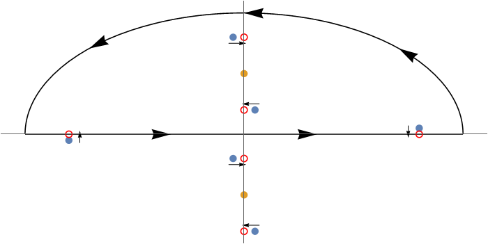
Figure 1: Pole structure of the integrand of the right hand side of equation (67).

The part of the Green’s function due to the bound states does not contribute to the asymptotic behavior, and it can be safely ignored since we take $\omega$ above the gap ($\omega>\nu_{B}+\omega_{0}$).

Thus, we have to evaluate the integral of the right hand side of equation (67) for $x\to\pm\infty$. The integrand is a meromorphic function of $k_{x}^{\prime}$ that decays exponentially to zero as $|k_{x}^{\prime}|\to\infty$ on the upper half complex plane if $x>x^{\prime}$, and on the lower half plane if $x<x^{\prime}$, due to the form of $\phi_{k_{x}^{\prime}}(x)$. Therefore the integral can be evaluated by the method of residues, choosing an integration contour as in figure 1 for $x>x^{\prime}$.

The generic pole structure of the integrand, which is analyzed with some detail in appendix B, is displayed in figure 1. There are two poles coming from $\phi_{k_{x}^{\prime}}(x)\phi_{k_{x}^{\prime}}^{*}(x^{\prime})$, located on the imaginary axis at $\pm\mathrm{i}q_{0}$ (yellow points). In addition, there are six more poles (blue points), three of them on the upper half plane and another three on the lower half plane (see figure 1). As $\mu\to 0^{+}$ two of these six poles attain the real axis, at the solutions $k_{x}^{\prime}=\pm k_{x}$ of the equation $\sqrt{\omega_{1}\omega_{2}}=\omega$ (see appendix B) The negative pole $-k_{x}$ is reached from the lower half plane and the positive pole $k_{x}$ from the upper half plane. All the other poles remain separated from the real axis as $\mu\to 0^{+}$ (see the red circles in Figure 1).

Consider the case $x>x^{\prime}$. For $x-x^{\prime}\to\infty$ the contribution of poles which do not attain the real axis as $\mu\to 0^{+}$ is exponentially small and do not contribute to the asymptotic behaviour, which is given only by the $k_{x}$ pole. Its residue can be readily computed and gives the asymptotic part, as $x\to\infty$, keeping $x^{\prime}$ fixed, of the Green’s function

$$G_{\mathrm{as}}^{+}(x,x^{\prime},-\mathrm{i}\omega)=-\frac{\mathrm{i}}{v_{x}}\mathrm{e}^{\mathrm{i}\delta_{0}}\mathrm{e}^{\mathrm{i}k_{x}x}\phi_{k_{x}}^{*}(x^{\prime})P_{m},$$ (68)

where $v_{x}=\partial\omega/\partial k_{x}$ is the group velocity, and

$$P_{m}=\frac{1}{2}\begin{pmatrix}1&-\mathrm{i}\sqrt{\omega_{2}/\omega_{1}}\\ \mathrm{i}\sqrt{\omega_{1}/\omega_{2}}&1\end{pmatrix}$$ (69)

is the projector along $\xi_{p}$ onto $\xi_{m}$:

$$P_{m}\,\xi_{p}=0,\quad P_{m}\,\xi_{m}=\xi_{m}.$$ (70)

One has to bear in mind that in equation (68) $\omega_{1}$ and $\omega_{2}$ depend on $k_{x}$ and that $\omega$ and $k_{x}$ are related by the equation $\omega_{1}\omega_{2}=\omega^{2}$ (the dispersion relation) which then determines the group velocity.

For $x-x^{\prime}<0$ we have to close the integral contour on the lower half plane and again only the pole attaining the real axis (this time at $k_{x}^{\prime}=-k_{x}$) as $\mu\to 0^{+}$ contributes to the asymptotic behavior $x-x^{\prime}\to-\infty$. The asymptotic Green’s function as $x\to-\infty$ with $x^{\prime}$ fixed is given by

$$G_{\mathrm{as}}^{+}(x,x^{\prime},-\mathrm{i}\omega)=\frac{\mathrm{i}}{v_{x}}\mathrm{e}^{\mathrm{i}\delta_{0}}\mathrm{e}^{-\mathrm{i}k_{x}x}\phi_{k_{x}}(x^{\prime})P_{m}.$$ (71)

VII Distorted wave Born approximation

We get an approximation to $\xi_{k_{x}}^{+}(x)$ by using the first (distorted wave) Born approximation to solve the Lippmann-Schwinger equation, substituting on its right-hand-side $\xi_{k_{x}}(x^{\prime\prime})$ by $\phi_{k_{x}}(x^{\prime\prime})\,\xi_{m}$:

$$\begin{split}\xi_{k_{x}}^{+}(x)=\phi_{k_{x}}(x)\,\xi_{m}+\int_{-\infty}^{\infty}dx^{\prime}G^{+}(x,x^{\prime},-\mathrm{i}\omega+\mu)\times\\ \int_{-\infty}^{\infty}dx^{\prime\prime}\epsilon\omega_{0}V(x^{\prime},x^{\prime\prime})\,\phi_{k_{x}}(x^{\prime\prime})\,\xi_{m}.\hskip 22.76228pt\end{split}$$ (72)

We expect the Born approximation will be good if $\epsilon q_{0}/k_{x}$ is small enough, since the correction to the wave function introduced by the perturbation considered here is of this order. It is well known that in one dimensional problems the Born approximation cannot be used in the vicinity of the gap frequency (small $k_{x}$), since the Green’s function diverges for $k_{x}\to 0$ (see reference LandauQM, ).

The scattering properties (reflection and transmission amplitudes) are obtained in the Born approximation from the explicit expression for $\xi_{k_{x}}^{+}(x)$ given by equation (72).

VII.1 The $x\to\infty$ asymptotics

For $x\to\infty$ we can substitute the Green’s function by the corresponding asymptotic Green’s function, given by equation (68). We can neglect the contribution to the integral in $dx^{\prime}$ of the region in which $x^{\prime}$ is of the order of, or larger than, $x$, since

$$\int_{-\infty}^{\infty}dx^{\prime\prime}\epsilon\omega_{0}V(x^{\prime},x^{\prime\prime})\,\phi_{k_{x}}(x^{\prime\prime})$$ (73)

tends to zero exponentially as $x^{\prime}\to\infty$. This is due to the fact that the perturbation $V$ is a localized operator. Using the asymptotic form of $\phi_{k_{x}}(x)$ and $G_{\mathrm{as}}^{+}$ given by equation (68), we get for $x\to\infty$

$$\xi_{k_{x}}^{+}(x)\sim-\mathrm{i}\mathrm{e}^{\mathrm{i}\delta_{0}}\mathrm{e}^{\mathrm{i}k_{x}x}\xi_{m}-\frac{\mathrm{i}\epsilon\omega_{0}}{v_{x}}\mathrm{e}^{\mathrm{i}\delta_{0}}\mathrm{e}^{\mathrm{i}k_{x}x}P_{m}\mathcal{T}\xi_{m},$$ (74)

where the $2\times 2$ matrix $\mathcal{T}$ depends only on $k_{x}$ and $k_{z}$ and is given by

$$\mathcal{T}=\int_{-\infty}^{\infty}dx^{\prime}\phi_{k_{x}}^{*}(x^{\prime})\int_{-\infty}^{\infty}dx^{\prime\prime}V(x^{\prime},x^{\prime\prime})\phi_{k_{x}}(x^{\prime\prime}).$$ (75)

Taking into account the form of $V(x^{\prime},x^{\prime\prime})$, the matrix elements $t_{ij}$ of $\mathcal{T}$ are given by the integrals

$$t_{ij}=\int dx^{\prime}\int dx^{\prime\prime}\phi_{k_{x}}^{*}(x^{\prime})f_{ij}(x^{\prime},x^{\prime\prime},k_{z})\phi_{k_{x}}(x^{\prime\prime}),$$ (76)

where

$$f_{11}=\mathrm{i}\,\sigma(k_{z})\sin\theta(x^{\prime})\sigma(x^{\prime}-x^{\prime\prime})\rho(x^{\prime}-x^{\prime\prime}),$$ (77)

$$f_{12}=-\sin\theta(x^{\prime})\rho(x^{\prime}-x^{\prime\prime})\sin\theta(x^{\prime\prime}),$$ (78)

$$f_{21}=d(x^{\prime}-x^{\prime\prime}),$$ (79)

$$f_{22}=-\mathrm{i}\,\sigma(k_{z})\sigma(x^{\prime}-x^{\prime\prime})\rho(x^{\prime}-x^{\prime\prime})\sin\theta(x^{\prime\prime}).\hskip 14.22636pt$$ (80)

Since $P_{m}$ projects onto $\xi_{m}$, we have $P_{m}\mathcal{T}\xi_{m}=\chi_{t}\xi_{m}$, where $\chi_{t}$ is a complex number that can be computed in terms of the $t_{ij}$:

$$\chi_{t}=\frac{\mathrm{i}}{2}\big{(}\sqrt{\omega_{1}/\omega_{2}}\,t_{12}-\sqrt{\omega_{2}/\omega_{1}}\,t_{21}\big{)}.$$ (81)

In deriving the above expression we used the fact that, by symmetry, $t_{11}+t_{22}=0$. Furthermore, the integrals that define $t_{12}$ and $t_{21}$ can be evaluated explicitely in terms of the derivative of the digamma function. The explicit expressions are given in appendix C.

Summarizing, we have obtained that for $x\to\infty$

$$\xi_{k_{x}}^{+}(x)\sim-\mathrm{i}\mathrm{e}^{\mathrm{i}\delta_{0}}\Big{(}1+\frac{\epsilon\omega_{0}}{v_{x}}\chi_{t}\Big{)}\mathrm{e}^{\mathrm{i}k_{x}x}\xi_{m}.$$ (82)

VII.2 The $x\to-\infty$ asymptotics

For $x\to-\infty$ we can substitute the Green’s function by the corresponding asymptotic Green’s function, given by equation (71), and we can neglect the contribution to the integral in $dx^{\prime}$ of the region in which $|x^{\prime}|$ is of the order of, or larger than, $|x|$, since $V$ is a localized operator. Using the asymptotic form of $\phi_{k_{x}}(x)$ and $G_{\mathrm{as}}^{+}$ given by equation (71), we get for $x\to-\infty$

$$\xi_{k_{x}}^{+}(x)\sim-\mathrm{i}\mathrm{e}^{-\mathrm{i}\delta_{0}}\mathrm{e}^{\mathrm{i}k_{x}x}\xi_{m}+\frac{\mathrm{i}\epsilon\omega_{0}}{v_{x}}\mathrm{e}^{\mathrm{i}\delta_{0}}\mathrm{e}^{-\mathrm{i}k_{x}x}P_{m}\mathcal{R}\xi_{m},$$ (83)

where the $2\times 2$ matrix $\mathcal{R}$ depends only on $k_{x}$ and $k_{z}$ and is given by

$$\mathcal{R}=\int_{-\infty}^{\infty}dx^{\prime}\phi_{k_{x}}(x^{\prime})\int_{-\infty}^{\infty}dx^{\prime\prime}V(x^{\prime},x^{\prime\prime})\phi_{k_{x}}(x^{\prime\prime}).$$ (84)

Taking into account the form of $V(x^{\prime},x^{\prime\prime})$, the matrix elements $r_{ij}$ of $\mathcal{R}$ are given by

$$r_{ij}=\int dx^{\prime}\int dx^{\prime\prime}\phi_{k_{x}}(x^{\prime})f_{ij}(x^{\prime},x^{\prime\prime},k_{z})\phi_{k_{x}}(x^{\prime\prime}),$$ (85)

with the functions $f_{ij}$ defined by equations (77)-(80).

Since $P_{m}$ projects onto the subspace spanned by $\xi_{m}$, we have $P_{m}\mathcal{R}\xi_{m}=\chi_{r}\xi_{m}$, where $\chi_{r}$ is a complex number that can be computed in terms of the $r_{ij}$:

$$\chi_{r}=\frac{1}{2}\big{(}r_{11}+r_{22}\big{)}+\frac{\mathrm{i}}{2}\big{(}\sqrt{\omega_{1}/\omega_{2}}r_{12}-\sqrt{\omega_{2}/\omega_{1}}r_{21}\big{)}.$$ (86)

Hence we have that for $x\to-\infty$

$$\xi_{k_{x}}^{+}(x)\sim-\mathrm{i}\mathrm{e}^{-\mathrm{i}\delta_{0}}\mathrm{e}^{\mathrm{i}k_{x}x}\xi_{m}+\frac{\mathrm{i}\epsilon\omega_{0}}{v_{x}}\chi_{r}\mathrm{e}^{\mathrm{i}\delta_{0}}\mathrm{e}^{-\mathrm{i}k_{x}x}\xi_{m},$$ (87)

VII.3 The scattering parameters

Inspecting equations (87) and (82) we see that by multiplying $\xi_{k_{x}}^{+}$ by $\mathrm{i}\mathrm{e}^{\mathrm{i}\delta_{0}}$ we get the asymptotic behavior

$$\xi_{k_{x}}^{+}(x)\sim\mathrm{e}^{\mathrm{i}k_{x}x}+R\,\mathrm{e}^{-\mathrm{i}k_{x}x},\quad\xi_{k_{x}}^{+}(x)\sim T\,\mathrm{e}^{\mathrm{i}k_{x}x},$$ (88)

for $x\to-\infty$ and $x\to+\infty$, respectively, where

$$R=-\frac{\epsilon\omega_{0}}{v_{x}}\mathrm{e}^{\mathrm{i}2\delta_{0}}\chi_{r},\quad T=\mathrm{e}^{\mathrm{i}2\delta_{0}}\Big{(}1-\frac{\epsilon\omega_{0}}{v_{x}}\chi_{t}\Big{)},$$ (89)

are the reflection and transmission amplitudes, respectively. Thus, in the Born approximation the reflection coefficient is

$$|R|=\epsilon\frac{\omega_{0}}{v_{x}}|\chi_{r}|,$$ (90)

while the transmission coefficient is, to this order of approximation, $|T|=1$, since $\chi_{t}$ is purely imaginary. The reflected and transmitted waves pick up phases, $\varphi_{r}$ and $\varphi_{t}$, respectively, with respect to the incident wave, which are given by

$$\varphi_{r}=2\delta_{0}+\delta\varphi_{r},\quad\varphi_{t}=2\delta_{0}+\epsilon\delta\varphi_{t},$$ (91)

where

$$\delta\varphi_{r}=\pi+\atan\Big(\frac{\sqrt{\omega_{1}/\omega_{2}}r_{12}-\sqrt{\omega_{2}/\omega_{1}}r_{21}}{r_{11}+r_{22}}\Big{missing}),$$ (92)

$$\delta\varphi_{t}=\frac{\omega_{0}}{2v_{x}}\big{(}\sqrt{\omega_{1}/\omega_{2}}\,t_{12}-\sqrt{\omega_{2}/\omega_{1}}\,t_{21}\big{)}.$$ (93)

The dependence of the phases on the wave vector originates a shift of the center of the scattered wave packets, with respect to the center of the incident wave packet, given by

$$\delta x_{l}=-\frac{\partial\varphi_{l}}{\partial k_{x}},\quad\delta z_{l}=-\frac{\partial\varphi_{l}}{\partial k_{z}},$$ (94)

where the subscript $l$ stands either for $r$ (reflected) or for $t$ (transmitted). These relations are obtained from a stationary phase analysis, and imply that the scattered waves propagate along lines shifted laterally with respect to the prediction of the geometrical optics limit by an amount given by

$$\delta s_{r}=\sin\alpha\frac{\partial\varphi_{r}}{\partial k_{x}}+\cos\alpha\frac{\partial\varphi_{r}}{\partial k_{z}},$$ (95)

$$\delta s_{t}=\sin\alpha\frac{\partial\varphi_{t}}{\partial k_{x}}-\cos\alpha\frac{\partial\varphi_{t}}{\partial k_{z}},$$ (96)

where $\alpha$ is the incidence angle: $\alpha=\atan(v_{z}/v_{x})$, with $v_{z}=\partial\omega/\partial k_{z}$.

The reflection coefficient vanishes at normal incidence ($k_{z}=0$), as can be seen by a careful analysis of the integrals (85), and thus in this case all the energy carried by the spin wave is transmitted. The contribution of the dipolar interaction to the transmitted amplitude also vanishes at normal incidence, as can be seen from equations (115) and (116). It is however interesting that even in this case the transmitted wave is shifted laterally from the incidence direction, since $\partial t_{21}/\partial k_{z}$ does not vanish at $k_{z}=0$. To order $\epsilon$, the amount of the lateral shift at normal incidence is given by

$$\begin{split}\delta s_{t}=\frac{\epsilon}{4k_{x}}\frac{q_{0}^{4}}{k_{x}^{2}+q_{0}^{2}}\left[\frac{2}{(\mathrm{i}k_{x}-4q_{0})^{2}}+\frac{2}{(\mathrm{i}k_{x}-2q_{0})^{2}}\right.\\ \left.-\frac{1}{k_{x}^{2}}-\frac{1}{2q_{0}^{2}}\psi^{\prime}\Big{(}\frac{\mathrm{i}k_{x}-4q_{0}}{2q_{0}}\Big{)}+c.c.\right].\end{split}$$ (97)

Clearly, by symmetry the shift at normal incidence should vanish in the case of a 360^o wall, and indeed it has been shown that it does vanish in the case of the chiral soliton of monoaxial helimagnets Laliena2021 . But symmetry is absent in the case of the 180^o domain wall considered here, since the spin wave propagates between two domains with opposite magnetizations. Hence, as we have seen, the lateral shift does not vanish at normal incidence. It has the direction of the magnetization of the domain to which the wave is transmitted (in our coordinate system, the $-{\boldsymbol{z}}$ direction).

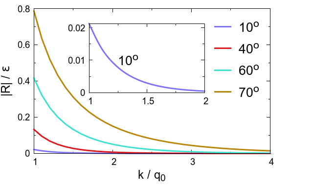
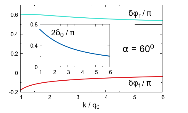
Figure 2: Reflection coefficient (left) for the incidence angles indicated in the legend and phases of the scattered waves (right) for incidence angle $\alpha=60^{\mathrm{o}}$.

VII.4 Some results

Let us discuss some results obtained by numerical evaluation of the integrals (85), and of the right-hand-side of equations (115) and (116) given in appendix C.

Let $k_{x}=k\cos\alpha$ and $k_{z}=k\sin\alpha$, where $k$ is the modulus of the wave vector and $\alpha$ the incidence angle. Figure 2 (left) displays the reflection coefficient $|R|/\epsilon$ as a function of $k$ for several values of the incidence angle. Actually, we plot the limit $\epsilon\to 0$ of $|R|/\epsilon$, since we consider $\epsilon$ small. As discussed in the previous section, the reflection coeficient vanishes at normal incidence ($\alpha=0$). We see from Figure 2 (left) that $|R|/\epsilon$ is very small for $\alpha=10^{\mathrm{o}}$.

Figure 2 (right) displays the phases of the scattered waves induced by the dipolar interaction, $\delta\varphi_{r}$ and $\delta\varphi_{t}$, for incidence angle $\alpha=60^{\mathrm{o}}$. The inset shows the phase shift in absence of dipolar interaction, $2\delta_{0}$. Again, we keep only the first order in $\epsilon$ and consequently we set $\epsilon=0$ in $\delta\varphi_{r}$ and $\delta\varphi_{t}$ [see the definitions (91)]. We see that $\varphi_{r}\to\pi/2$ as $k\to\infty$ (since $\delta_{0}\to 0$), as it happens to be usually for reflected waves. Analogously, we see that $\varphi_{t}\to 0$ as $k\to\infty$, as it is expected for a transmitted wave.

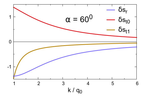
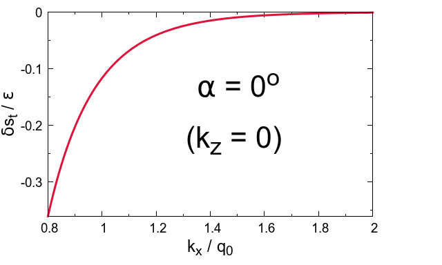
Figure 3: Lateral shift of the scattered waves at incidence angle $\alpha=60^{\mathrm{o}}$ (left) and at normal incidence, $\alpha=0^{\mathrm{o}}$ (right), in units of the domain wall width, $1/q_{0}$.

The left panel of Figure 3 shows the lateral shift of the scattered waves, in units of the domain wall width, $1/q_{0}$, as a function of the wave number $k$ for $\alpha=60^{\mathrm{o}}$. To avoid choosing a particular value of $\epsilon$, we use equation (91) to split the shift of the transmitted wave as $\delta s_{t}=\delta s_{t0}+\epsilon\delta s_{t1}$, where $\delta s_{t0}$ comes from the $2\delta_{0}$ contribution to $\varphi_{t}$ and $\delta s_{t1}$ comes from the $\delta\varphi_{t}$ term of $\varphi_{t}$. The figure displays $\delta s_{t0}$ and $\delta s_{t1}$, with $\epsilon=0$ in this last quantity. The two terms have opposite signs and therefore tend to cancel, but the degree of cancellation depends on $\epsilon$. It is seen that the shifts are of the order of the wavelength for $k$ of the order of $q_{0}$ (i.e., for wavelengths of the order of the domain wall width), and vanish as $k\to\infty$, as expected. If the reflection coefficient is small enough, and this depends on the actual value of $\epsilon$, the shift of the transmitted waves can be enhanced by making the spin wave propagate through an array of well separated domain walls, since the shift is clearly additive.

The lateral shift for normal incidence, in units of $1/q_{0}$, is shown as a function of the wave number, $k_{x}$, in Figure 3 (right). Again, to avoid choosing a value for $\epsilon$ we actually plot the limit $\epsilon\to 0$ of $\delta s_{t}/\epsilon$. We see that it is negative, what means that the transmitted wave at normal incidence is shifted laterally towards the direction of the magnetization of the domain into which the spin wave is transmitted (the $-{\boldsymbol{z}}$ direction in our coordinate system). The shift decreases with the wave number, and it is a fraction of the wavelength. Its actual size is proportional to $\epsilon$. Given that the reflection coefficient vanish at normal incidence, the lateral shift of the transmitted wave might be greatly enhanced by using an array of well separated domain walls. The existence of this shift may be an interesting tool to control and manipulate the spin waves.

VIII Conclusions

If the dipolar interaction is neglected, or if it is approximated by a local effective anisotropy field, the theoretical computations show that a Bloch domain wall of an anisotropic ferromagnet is transparent to spin waves Braun1994 ; Winter1961 ; Thiele1973 . However, we have shown in this paper that if the dipolar interaction is taken into account properly the spin waves are actually reflected by a Bloch domain wall. The scattering parameters have been obtained perturbatively, using the distorted wave Born approximation. The application of this perturbative tecnique is not straightforward, due to the non localized character of the dipolar interaction. It is necessary to split the dipolar contribution to the spin wave operator into two terms: an operator that can be absorbed into the term treated exactly and an operator which is localized and can be treated perturbatively in the first (distorted wave) Born approximation.

The scattering parameters can be computed within this distorted wave Born approximation. It turns out that the reflection coefficient vanishes only for normal incidence. The phase shifts are different for the transmitted and reflected waves, due to the fact that the wall separates two domains with opposite magnetization, and therefore the mirror symmetry about the wall plane is broken. The phase shifts depend not only on the wave vector component perpendicular to the wall plane but also on the component parallel to the wall plane. The dependence of the phase shifts on the wave vector induce a lateral shift of the reflected and transmitted waves. It is worthwhile to stress that the lateral shift of the transmitted wave does not vanish at normal incidence, due to the lack of symmetry caused by the reversal of the magnetization between the two domains separated by the wall. In this case the shift has the direction of the magnetization of the domain to which the spin wave is transmitted. Since the reflection coefficient vanish at normal incidence, this shift can be greatly enhanced by forcing the spin wave to go through an array of well separated domain walls. These properties of the scattering by a domain wall may be very useful to control the spin waves.

Acknowledgements

Grant Number PGC2018099024B100 funded by MCIN/AEI/10.13039/501100011033 supported this work. Grants OTR02223 from CSIC/MICIN and DGA/M4 from Diputación General de Aragón (Spain) are also acknowledged.

Appendix A

In this appendix we giev some details on the derivation of the $\tilde{D}_{\alpha\beta}$ which gives the contribution of the dipolar interaction to the spin wave operator. It is studied in section IV. Equation (32) shows that the dipolar field $\delta\boldsymbol{h}_{d}$ created by the perturbation $\delta{\boldsymbol{n}}$ has the form of a convolution between the Coulomb potential $\boldsymbol{r}/r^{3}$ and

$$\nabla\dotproduct\delta{\boldsymbol{n}}=\partial_{x}\xi_{1}+\cos\theta(x)\partial_{y}\xi_{2}-\sin\theta(x)\partial_{z}\xi_{2}.$$ (98)

Therefore, in terms of the Fourier transform of $\xi_{\alpha}$ with respect to $y$ and $z$, given by (33), the dipolar field at point $\boldsymbol{r}=x{\boldsymbol{x}}+\boldsymbol{r}_{p}$ has the form

$$\delta\boldsymbol{h}_{d}\!=\!-\!\int\!\frac{d^{2}k_{p}}{(2\pi)^{2}}\mathrm{e}^{\mathrm{i}\boldsymbol{k}_{p}\dotproduct\boldsymbol{r}_{p}}\!\!\int dx^{\prime}\boldsymbol{C}(x-x^{\prime},\boldsymbol{k}_{p})M(x^{\prime},\boldsymbol{k}_{p}),$$ (99)

where

$$M(x^{\prime},\boldsymbol{k}_{p})=\partial_{x^{\prime}}\tilde{\xi}_{1}(x^{\prime},\boldsymbol{k}_{p})+\mathrm{i}k_{p}F(x^{\prime},\boldsymbol{k}_{p})\tilde{\xi}_{2}(x^{\prime},\boldsymbol{k}_{p}),$$ (100)

with $F(x,\boldsymbol{k}_{p})$ given by equation (41), and

$$\boldsymbol{C}(x,\boldsymbol{k}_{p})=\frac{1}{4\pi}\int d^{2}r_{p}\,\mathrm{e}^{-\mathrm{i}\boldsymbol{k}_{p}\dotproduct\boldsymbol{r}_{p}}\frac{x{\boldsymbol{x}}+\boldsymbol{r}_{p}}{\big{(}x^{2}+r_{p}^{2}\big{)}^{3/2}}.$$ (101)

The above expression can be written as

$$\boldsymbol{C}(x,\boldsymbol{k}_{p})=xA(x,\boldsymbol{k}_{p}){\boldsymbol{x}}+\mathrm{i}\nabla_{k_{p}}A(x,\boldsymbol{k}_{p}),$$ (102)

where

$$A(x,\boldsymbol{k}_{p})=\frac{1}{4\pi}\int d^{2}r_{p}\,\mathrm{e}^{-\mathrm{i}\boldsymbol{k}_{p}\dotproduct\boldsymbol{r}_{p}}\frac{1}{\big{(}x^{2}+r_{p}^{2}\big{)}^{3/2}}.$$ (103)

For $x\neq 0$ this integral can be readily performed and is equal to

$$A(x,\boldsymbol{k}_{p})=\frac{1}{2}\frac{\mathrm{e}^{-k_{p}|x|}}{|x|}.$$ (104)

From this and (102) we obtain

$$\boldsymbol{C}(x,\boldsymbol{k}_{p})=\frac{1}{2}\sigma(x)\mathrm{e}^{-k_{p}|x|}{\boldsymbol{x}}-\mathrm{i}\frac{1}{2}\mathrm{e}^{-k_{p}|x|}\frac{\boldsymbol{k}_{p}}{k_{p}}.$$ (105)

Inserting the above expression into (99) and integrating by parts the term that involves $\partial_{x^{\prime}}\tilde{\xi}_{1}$, taking into account that the boundary term vanishes since $\tilde{\xi}_{1}$ vanishes for large $|x|$, and that $d\sigma(x)/dx=2\delta(x)$, we get

$$\delta\boldsymbol{h}_{d}=-\int\frac{d^{2}k_{p}}{(2\pi)^{2}}\,\mathrm{e}^{\mathrm{i}\boldsymbol{k}_{p}\dotproduct\boldsymbol{r}_{p}}\int dx^{\prime}\boldsymbol{\Upsilon}(x,x^{\prime},\boldsymbol{k}_{p}),$$ (106)

where

$$\boldsymbol{\Upsilon}(x,x^{\prime},\boldsymbol{k}_{p})={\boldsymbol{x}}\,\Theta(x,x^{\prime},\boldsymbol{k}_{p})+\frac{\boldsymbol{k}_{p}}{k_{p}}\,\Phi(x,x^{\prime},\boldsymbol{k}_{p}),$$ (107)

width

$$\begin{split}\Theta(x,x^{\prime},\boldsymbol{k}_{p})=\Big{(}\delta(x-x^{\prime})-\rho(x-x^{\prime})\Big{)}\tilde{\xi}_{1}(x^{\prime},\boldsymbol{k}_{p})\\ +\mathrm{i}\sigma(x-x^{\prime})\rho(x-x^{\prime})F(x^{\prime},\boldsymbol{k}_{p})\tilde{\xi}_{2}(x^{\prime},\boldsymbol{k}_{p}),\hskip 11.38092pt\end{split}$$ (108)

$$\begin{split}\Phi(x,x^{\prime},\boldsymbol{k}_{p})=\mathrm{i}\sigma(x-x^{\prime})\rho(x-x^{\prime})\tilde{\xi}_{1}(x^{\prime},\boldsymbol{k}_{p})\\ +\rho(x-x^{\prime})F(x^{\prime},\boldsymbol{k}_{p})\tilde{\xi}_{2}(x^{\prime},\boldsymbol{k}_{p}).\hskip 22.76228pt\end{split}$$ (109)

From equations (106)-(109) it is straightforward to obtain $\tilde{D}_{\alpha\beta}$ using equations (15) and (16).

Appendix B

Let us analyze the pole structure in $k_{x}^{\prime}$ of the integrand entering the right hand side of equation (67). There are two poles coming from $\phi_{k_{x}^{\prime}}(x)\phi_{k_{x}^{\prime}}^{*}(x^{\prime})$, located on the imaginary axis, given by $\pm\mathrm{i}q_{0}$ (golden points in Figure 1). The contribution of these to poles to the integral gives a function exponentially decreasing with $|x-x^{\prime}|$ and thus it vanishes asymptotically. They do not contribute to the asymptotic part of the Green’s function.

Let introduce the variable $z=k_{x}^{\prime\,2}$. The other poles come from the zeros of

$$f(z)=\omega_{1}(z)\omega_{2}(z)+(-\mathrm{i}\omega+\mu)^{2}.$$ (110)

Let us consider first the case $k_{z}\neq 0$. Since $z=-k_{z}^{2}$ is a pole of $f(z)$, it is clear that $p(z)=(z+k_{z}^{2})f(z)$ has the same zeros as $f(z)$. But $p(z)$ is a polynomial of third degree and therefore it has three roots. Hence, $f(z)$ has exactly three zeros, which are the solutions of

$$g(z)=\omega^{2}+2\omega\mu\mathrm{i}-\mu^{2},$$ (111)

where, for convenience, we define $g(z)=\omega_{1}(z)\omega_{2}(z)$.

Only the poles which attain the real axis as $\mu\to 0^{+}$ do contribute to the asymptotic behavior of the Green’s function (see section VI). This means that we only need the zeros of $f(z)$ which attain the positive real axis as $\mu\to 0^{+}$. Let us set $\mu=0$ in equation (111). We notice two facts: i) $g(0)=\omega_{G}^{2}$; and ii) it is straightforward to see that $g^{\prime}(z)>0$ for $z\geq 0$, where the prime stands for the derivative. Therefore the equation $g(z)=\omega^{2}$ has one and only one solution on the positive real axis if $\omega\geq\omega_{G}$, and it has no real positive solution if $\omega<\omega_{G}$. The other two zeros of $f(z)$ are either non real or negative in the limit $\mu\to 0^{+}$.

Let us consider a frequency $\omega\geq\omega_{G}$ and let us denote by $z=k_{x}^{2}$ the unique positive solution of $g(z)=\omega^{2}$. For $\mu>0$ and small we can obtain the solution of equation (111) as a power series of $\mu$. To leading order we get

$$z=k_{x}^{2}+\mathrm{i}\frac{2\omega\mu}{g^{\prime}(k_{x}^{2})}+O(\mu^{2}).$$ (112)

For $\mu\to 0^{+}$ the imaginary part of the above expression is positive. This zero of $f(z)$ gives rise to the two poles that contribute to the asymptotic part of the Green’s function:

$$k_{x}^{\prime}=\pm\left(k_{x}+\mathrm{i}\frac{\omega\mu}{k_{x}g^{\prime}(k_{x}^{2})}\right).$$ (113)

One of the poles is located on the upper right quadrant of the complex plane and another one on the lower left quadrant of the complex plane.

The case $k_{z}=0$ is simpler, since then $g(z)$ is a polynomial of second degree and its zeros have a relatively simple explicit expression. For $\mu>0$ and small we obtain the two poles

$$k_{x}^{\prime}=\pm\left(k_{x}+\mathrm{i}\frac{\omega\mu}{k_{x}[\omega^{2}-\omega_{G}^{2}+\omega_{0}^{2}(1+\epsilon/2)^{2}]}\right).\vspace{2pt}$$ (114)

Again one of the poles is located on the upper right quadrant of the complex plane and another one on the lower left quadrant of the complex plane. Both attain the real axis as $\mu\to 0^{+}$.

Appendix C

The coefficients $t_{12}$ and $t_{21}$ defined by equations (76), (78), and (79) can be evaluated in terms of the derivative of the digamma function, $\psi^{\prime}(z)$. Let us remember that the digamma function, $\psi(z)$, is the derivative of the logarithm of the Gamma function. Defining the complex variable $\lambda=(|k_{z}|+\mathrm{i}k_{x})/q_{0}$, the explicit expressions are

$$t_{12} = -\frac{2k_{z}^{2}}{q_{0}\left(q_{0}^{2}+k_{x}^{2}\right)}\left[1+\frac{k_{z}}{q_{0}}\left(\frac{1}{(\lambda-3)^{2}}+\frac{1}{(\lambda-1)^{2}}-\frac{1}{4}\psi^{\prime}\Big{(}\frac{\lambda-3}{2}\Big{)}+c.c.\right)\right],$$ (115)

$$t_{21} = -\frac{k_{z}}{q_{0}^{2}+k_{x}^{2}}\left[\frac{2}{(\lambda-4)^{2}}+\frac{2}{(\lambda-2)^{2}}+\frac{q_{0}+k_{z}}{q_{0}\lambda^{2}}-\frac{1}{2}\psi^{\prime}\Big{(}\frac{\lambda-4}{2}\Big{)}+c.c.\right].$$ (116)

References

• [1] P. Pirro, V.I. Vasyuchka, A.A. Serga, and B. Hillebrands. Advances in coherent magnonics. Nature Reviews Materials, 6(12):1114–1135, 2021.
• [2] A. Barman, G. Gubbiotti, S. Ladak, et al. The 2021 magnonics roadmap. Journal of Physics Condensed Matter, 33(41), 2021.
• [3] H. Yu, J. Xiao, and H. Schultheiss. Magnetic texture based magnonics. Physics Reports, 905:1–59, 2021.
• [4] A. V. Chumak, V. I. Vasyuchka, A. A. Serga, and B. Hillebrands. Magnon spintronics. Nature Phys, 11:453–461, 2015.
• [5] T. Schneider, A. A. Serga, B. Leven, B. Hillebrands, R. L. Stamps, and M. P. Kostylev. Realization of spin-wave logic gates. Appl. Phys. Lett., 92:022505, 2008.
• [6] A. Khitun, M. Bao, and K.L. Wang. Magnonic logic circuits. Journal of Physics D: Applied Physics, 43(26), 2010.
• [7] A. V. Chumak, A. A. Serga, and B. Hillebrands. Magnon transistor for all-magnon data processing. Nature Commun, 5:4700, 2014.
• [8] Yu H et al. Magnetic thin-film insulator with ultra-low spin wave damping for coherent nanomagnonics. Scientific Reports, 4, 2014.
• [9] C. Hauser, T. Richter, N. Homonnay, C. Eisenschmidt, M. Qaid, H. Deniz, D. Hesse, M. Sawicki, S.G. Ebbinghaus, and G. Schmidt. Yttrium iron garnet thin films with very low damping obtained by recrystallization of amorphous material. Scientific Reports, 6, 2016.
• [10] C. Guillemard, S. Petit-Watelot, L. Pasquier, D. Pierre, J. Ghanbaja, J.-C. Rojas-Sánchez, A. Bataille, J. Rault, P. Le Fèvre, F. Bertran, and S. Andrieu. Ultralow Magnetic Damping in Co2Mn-Based Heusler Compounds: Promising Materials for Spintronics. Physical Review Applied, 11(6), 2019.
• [11] C.S. Davies, A. Francis, A.V. Sadovnikov, S.V. Chertopalov, M.T. Bryan, S.V. Grishin, D.A. Allwood, Y.P. Sharaevskii, S.A. Nikitov, and V.V. Kruglyak. Towards graded-index magnonics: Steering spin waves in magnonic networks. Physical Review B, 92(2), 2015.
• [12] C.S. Davies and V.V. Kruglyak. Graded-index magnonics. Low Temperature Physics, 41(10):760–766, 2015.
• [13] O. Dzyapko, I.V. Borisenko, V.E. Demidov, W. Pernice, and S.O. Demokritov. Reconfigurable heat-induced spin wave lenses. Applied Physics Letters, 109(23), 2016.
• [14] M. Vogel, A.V. Chumak, E.H. Waller, T. Langner, V.I. Vasyuchka, B. Hillebrands, and G. Von Freymann. Optically reconfigurable magnetic materials. Nature Physics, 11(6):487–491, 2015.
• [15] M. Vogel, R. Aßmann, P. Pirro, A.V. Chumak, B. Hillebrands, and G. von Freymann. Control of spin-wave propagation using magnetisation gradients. Scientific Reports, 8(1), 2018.
• [16] A. Bogdanov and A. Hubert. Thermodynamically stable magnetic vortex states in magnetic crystals. Journal of Magnetism and Magnetic Materials, 138:255, 1994.
• [17] S. Mühlbauer, B. Binz, F. Jonietz, C. Pfleiderer, A. Rosch, A. Neubauer, R. Georgii, and P. Böni. Skyrmion lattice in a chiral magnet. Science, 323(5916):915–919, 2009.
• [18] X.Z. Yu, Y. Onose, N. Kanazawa, J.H. Park, J.H. Han, Y. Matsui, N. Nagaosa, and Y. Tokura. Real-space observation of a two-dimensional skyrmion crystal. Nature, 465(7300):901–904, 2010.
• [19] V. Laliena and J. Campo. Stability of skyrmion textures and the role of thermal fluctuations in cubic helimagnets: a new intermediate phase at low temperature. Phys. Rev. B, 96:134420, 2017.
• [20] V. Laliena, G. Albalate, and J. Campo. Stability of the skyrmion lattice near the critical temperature in cubic helimagnets. Phys. Rev. B, 98:224407, 2018.
• [21] Y. Togawa, T. Koyama, T. Takayanagi, S. Mori, Y. Kousaka, J. Akimitsu, S. Nishihara, K. Inoue, A.S. Ovchinnikov, and J. Kishine. Chiral magnetic soliton lattice on a chiral helimagnet. Phys. Rev. Lett., 108:107202, 2012.
• [22] V. Laliena, J. Campo, and Y. Kousaka. Understanding the H-T phase diagram of the monoaxial helimagnet. Phys. Rev. B, 94:094439, 2016.
• [23] V. Laliena, J. Campo, and Y. Kousaka. Nucleation, instability, and discontinuous phase transitions in the phase diagram of the monoaxial helimagnet with oblique fields. Phys. Rev. B, 95:224410, 2017.
• [24] Yu. S. Dadoenkova, N. N. Dadoenkova, I. L. Lyubchanskii, M. L. Sokolovskyy, J. W. Kłos, J. Romero-Vivas, and M. Krawczyk. Huge Goos-Hänchen effect for spin waves: A promising tool for study magnetic properties at interfaces. Appl. Phys. Lett., 101:042404, 2012.
• [25] P. Gruszecki, J. Romero-Vivas, Yu. S. Dadoenkova, N. N. Dadoenkova, I. L. Lyubchanskii, and M. Krawczyk. Goos-Hänchen effect and bending of spin wave beams in thin magnetic films. Appl. Phys. Lett., 105:242406, 2014.
• [26] P. Gruszecki, M. Mailyan, O. Gorobets, and M. Krawczyk. Goos-Hänchen shift of a spin-wave beam transmitted through anisotropic interface between two ferromagnets. Phys. Rev. B, 95:014421, 2017.
• [27] M. Mailyan, P. Gruszecki, O. Gorobets, and M. Krawczyk. Goos-Hänchen Shift of a Spin-Wave Beam at the Interface Between Two Ferromagnets. IEEE Transactions on Magnetics, 53(11):1–5, 2017.
• [28] J. Stigloher, T. Taniguchi, H. S. Körner, M. Decker, T. Moriyama, T. Ono, and C. H. Back. Observation of a Goos-Hänchen-like Phase Shift for Magnetostatic Spin Waves. Phys. Rev. Lett., 121:137201, Sep 2018.
• [29] Zhenyu Wang, Yunshan Cao, and Peng Yan. Goos-Hänchen effect of spin waves at heterochiral interfaces. Phys. Rev. B, 100:064421, 2019.
• [30] Weiming Zhen and Dongmei Deng. Giant Goos-Hänchen shift of a reflected spin wave from the ultrathin interface separating two antiferromagnetically coupled ferromagnets. Optics Communications, 474:126067, 2020.
• [31] Klos, J.W. and Dadoenkova, Y.S. and Rychly, J. and Dadoenkova, N.N. and Lyubchanskii, I.L. and Barnaś, J. Hartman effect for spin waves in exchange regime. Scientific Reports, 8(1), 2018.
• [32] M. Golebiewski, P. Gruszecki, M. Krawczyk, and A.E. Serebryannikov. Spin-wave Talbot effect in a thin ferromagnetic film. Physical Review B, 102(13), 2020.
• [33] H.-B. Braun. Fluctuations and instabilities of ferromagnetic domain-wall pairs in an external magnetic field. Physical Review B, 50(22):16485–16500, 1994.
• [34] Christoph Schütte and Markus Garst. Magnon-skyrmion scattering in chiral magnets. Phys. Rev. B, 90:094423, 2014.
• [35] V. Laliena and J. Campo. Magnonic Goos-Hänchen Effect Induced by 1D Solitons. Advanced Electronic Materials, 2100782, 2021.
• [36] Riccardo Hertel, Wulf Wulfhekel, and Jürgen Kirschner. Domain-Wall Induced Phase Shifts in Spin Waves. Phys. Rev. Lett., 93:257202, 2004.
• [37] S.J. Hämäläinen, M. Madami, H. Qin, G. Gubbiotti, and S. van Dijken. Control of spin-wave transmission by a programmable domain wall. Nature Communications, 9(1), 2018.
• [38] N.L. Schryer and L.R. Walker. The motion of 180$\deg$ domain walls in uniform dc magnetic fields. Journal of Applied Physics, 45(12):5406–5421, 1974.
• [39] A. Thiaville, Y. Nakatani, J. Miltat, and Y. Suzuki. Micromagnetic understanding of current-driven domain wall motion in patterned nanowires. Europhys. Lett., 69:990–996, 2005.
• [40] S. Woo, K. Litzius, B. Krüger, M.-Y. Im, L. Caretta, K. Richter, M. Mann, A. Krone, R.M. Reeve, M. Weigand, P. Agrawal, I. Lemesh, M.-A. Mawass, P. Fischer, M. Kläui, and G.S.D. Beach. Observation of room-temperature magnetic skyrmions and their current-driven dynamics in ultrathin metallic ferromagnets. Nature Materials, 15(5):501–506, 2016.
• [41] V. Laliena, S. Bustingorry, and J. Campo. Dynamics of chiral solitons driven by polarized currents in monoaxial helimagnets. Sci Rep, 10:20430, 2020.
• [42] S.A. Osorio, V. Laliena, J. Campo, and S. Bustingorry. Creation of single chiral soliton states in monoaxial helimagnets. Applied Physics Letters, 119(22), 2021.
• [43] J.M. Winter. Bloch wall excitation. Application to nuclear resonance in a Bloch wall. Physical Review, 124(2):452–459, 1961.
• [44] A. A. Thiele. Excitation spectrum of magnetic domain walls. Physical Review B, 7:391–397, 1973.
• [45] Strictly speaking, we have to consider the energy density functional defined by $\mathcal{E}/L_{x}L_{y}L_{z}$.
• [46] C. Bayer, H. Schultheiss, B. Hillebrands, and R.L. Stamps. Phase shift of spin waves traveling through a 180o Bloch-domain wall. IEEE Transactions on Magnetics, 41(10):3094–3096, 2005.
• [47] J.-I. Kishine and A.S. Ovchinnikov. Canonical formulation of magnetic domain-wall motion. Physics Letters A, 375(17):1824–1830, 2011.
• [48] Pablo Borys, Felipe Garcia-Sanchez, Joo-Von Kim, and Robert L. Stamps. Spin Wave Eigenmodes of Dzyaloshinskii Domain Walls. Adv. Electron. Mater., 2:1500202, 2016.
• [49] N. J. Whitehead, S. A. R. Horsley, T. G. Philbin, A. N. Kuchko, and V. V. Kruglyak. Theory of linear spin wave emission from a Bloch domain wall. Phys. Rev. B, 96:064415, 2017.
• [50] P. G. Drazin and R. S. Johnson. Solitons: an introduction. Cambridge University Press, 1989.
• [51] F. Garcia-Sanchez, P. Borys, R. Soucaille, J.-P. Adam, R.L. Stamps, and J.-V. Kim. Narrow magnonic waveguides based on domain walls. Physical Review Letters, 114(24), 2015.
• [52] K. Wagner, A. Kákay, K. Schultheiss, A. Henschke, T. Sebastian, and H. Schultheiss. Magnetic domain walls as reconfigurable spin-wave nanochannels. Nature Nanotechnology, 11(5):432–436, 2016.
• [53] L. D. Landau and E. M. Lifshizt. Quantum Mechanics. Pergamon Press, 1991.