Computation of eigenfrequency sensitivities using Riesz projections for
efficient optimization of nanophotonic resonators

Abstract

Resonances are omnipresent in physics and essential for the description of wave phenomena. We present an approach for computing eigenfrequency sensitivities of resonances. The theory is based on Riesz projections and the approach can be applied to compute partial derivatives of the complex eigenfrequencies of any resonance problem. Here, the method is derived for Maxwell’s equations. Its numerical realization essentially relies on direct differentiation of scattering problems. We use a numerical implementation to demonstrate the performance of the approach compared to differentiation using finite differences. The method is applied for the efficient optimization of the quality factor of a nanophotonic resonator.

I Introduction

Resonance phenomena are ubiquitous in nanophotonics and play an important role for tailoring light-matter interactions Novotny and van Hulst (2011); Kuznetsov et al. (2016). They are exploited in, e.g., single-photon sources for quantum technology Senellart et al. (2017), biosensors Anker et al. (2008), nanolasers Ma and Oulton (2019), or solar energy devices Ma et al. (2016); Zhang et al. (2018). All these applications rely on the highly localized electromagnetic field energies in the vicinity of the underlying nanoresonators Lalanne et al. (2018). A central figure of merit for the description of resonance effects is the quality ($Q$) factor, which quantifies, in the case of low-loss systems, the relation between stored and radiated field energies of the resonances Wu et al. (2021). Nanoresonators with low energy dissipation, i.e., with high $Q$-factors, have been proposed to improve the efficiencies of nanophotonic devices West et al. (2010); Kuznetsov et al. (2016). For example, high-$Q$ resonators can boost the brightness of quantum emitters, the sensitivity of sensors, or the emission processes in plasmonic lasers Wang et al. (2021). Designing devices with numerical optimization is a time and cost effective approach. The resonances are numerically computed by solving the source-free Maxwell’s equations equipped with open boundary conditions Lalanne et al. (2019). This yields non-Hermitian eigenproblems and the solutions are eigenmodes with complex-valued eigenfrequencies. In this context, the $Q$-factor is defined as the scaled ratio of the real and imaginary parts of the eigenfrequency.

Nanoresonators with high $Q$-factors have been theoretically presented, but fabrication of these resonators is a limiting task Wang et al. (2021). The sensitivity analysis of eigenfrequencies can show a way to reduce the sensitivities of the $Q$-factors. This can support the nanofabrication processes. Furthermore, the sensitivity analysis of eigenfrequencies is essential for numerical simulation. For example, the numerical accuracies of the calculated eigenfrequencies are strongly influenced by the sensitivities of the eigenfrequencies when the systems are subject to small perturbations Bindel and Hood (2013); Güttel and Tisseur (2017). In particular, for high-$Q$ resonators, the accuracy requirements are demanding since the real and imaginary parts of the eigenfrequencies differ by several orders of magnitude. Sensitivities are also directly exploited in numerical optimization algorithms using gradients Jensen and Sigmund (2011), for gradient-enhanced surrogate modelling Bouhlel et al. (2019), and for local sensitivity analyses Cacuci et al. (2005). The computation of eigenfrequency sensitivities is usually based on perturbation theory Kato (1995); Sakurai and Napolitano (2020), where the sensitivity of the underlying operator, the left and the right eigenmodes, and a proper normalization of the eigenmodes are required. The solution of the perturbed systems, on the other hand, is not necessary. For resonance problems, left and right eigenmodes are in general not identical, which increases the computational effort, and normalization requires additional attention. There are specialized approaches that, e.g., exploit magnetic fields for extracting the left eigenmodes Burschäpers et al. (2011), introduce an adjoint system for computing sensitivities Swillam et al. (2008), or that rely on internal and external electric fields at the boundaries of the nanoresonators Yan et al. (2020). It is also possible to completely omit the use of eigenmodes for sensitivity analysis Alam and Safique Ahmad (2019). A further approach is the straightforward application of finite differences. However, this also includes the solution of the perturbed resonance problems, which increases the computational effort.

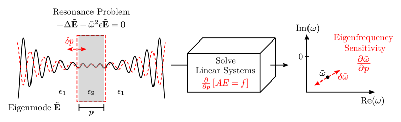
Figure 1: Schematic representation of computing eigenfrequency sensitivities of a resonator using contour integration. The system is defined by layers with different permittivities $\epsilon_{1}$ and $\epsilon_{2}$ and is described by the one-dimensional Helmholtz equation $-\Delta\tilde{\mathbf{E}}-\tilde{\omega}^{2}\epsilon\tilde{\mathbf{E}}=0$. A solution to the resonance problem is given by the eigenmode $\tilde{\mathbf{E}}$ and the corresponding complex-valued eigenfrequency $\tilde{\omega}\in\mathbb{C}$. The real part of the electric field of the eigenmode is sketched with the solid black curve. A perturbation $\delta p$ of the middle layer width $p$ leads to a perturbed electric field, represented by the dashed red curve, and to a perturbation $\delta\tilde{\omega}$ of the eigenfrequency. Computing contour integrals by solving linear systems $AE=f$ and $\partial/\partial p\left[AE=f\right]$ in the complex frequency plane yields the eigenfrequency sensitivity $\partial\tilde{\omega}/\partial p$. Solving the linear systems is considered as a blackbox.

In this work, we present an approach for computing eigenfrequency sensitivities that completely avoids solving resonance problems. The approach is based on Riesz projections given by contour integrals in the complex frequency plane. The contour integrals are numerically accessed by solving Maxwell’s equations with a source term enabling an efficient numerical realization using direct differentiation. The numerical experiments show a significant reduction in computational effort compared to applying finite differences. A Bayesian optimization algorithm with the incorporation of eigenfrequency sensitivities is used to optimize a resonator hosting a resonance with a high $Q$-factor.

II Theoretical background and numerical realization

We start with an introduction of the theoretical background on resonance phenomena occurring in nanophotonics. Based on this, Riesz projections for computing eigenfrequency sensitivities and an efficient approach for its numerical realization are presented.

II.1 Resonances in nanophotonics

In nanophotonics, in the steady-state regime, light-matter interactions can be described by the time-harmonic Maxwell’s equations in second-order form,

$$\nabla\times\mu_{0}^{-1}\nabla\times\mathbf{E}(\mathbf{r},\omega_{0})-\omega_{0}^{2}\epsilon(\mathbf{r},\omega_{0})\mathbf{E}(\mathbf{r},\omega_{0})=i\omega_{0}\mathbf{J}(\mathbf{r}),$$ (1)

where $\mathbf{E}(\mathbf{r},\omega_{0})\in\mathbb{C}^{3}$ is the electric field, $\mathbf{r}\in\mathbb{R}^{3}$ is the position, $\omega_{0}\in\mathbb{R}$ is the angular frequency, and $\mathbf{J}(\mathbf{r})\in\mathbb{C}^{3}$ is the electric current density corresponding to a light source. In the optical regime, the permeability tensor $\mu(\mathbf{r},\omega_{0})$ typically equals the vacuum permeability $\mu_{0}$. The permittivity tensor $\epsilon(\mathbf{r},\omega_{0})=\epsilon_{\mathrm{r}}(\mathbf{r},\omega_{0})\epsilon_{0}$, where $\epsilon_{\mathrm{r}}(\mathbf{r},\omega_{0})$ is the relative permittivity and $\epsilon_{0}$ the vacuum permittivity, describes the spatial distribution of material and the material dispersion. Solutions to Eq. (1) are called scattering solutions as light from a source is scattered by a material system.

Resonances are solutions to Eq. (1) without a source term, i.e., $\mathbf{J}(\mathbf{r})=0$, and with transparent boundary conditions. The boundary conditions lead to non-Hermitian eigenproblems, and, if material dispersion is also present, the eigenproblems become nonlinear. The electric field distribution of an eigenmode is denoted by $\tilde{\mathbf{E}}(\mathbf{r})\in\mathbb{C}^{3}$ and the corresponding complex-valued eigenfrequency by $\tilde{\omega}\in\mathbb{C}$. The $Q$-factor of a resonance is defined by

$$Q=\frac{\mathrm{Re}(\tilde{\omega})}{-2\mathrm{Im}(\tilde{\omega})}$$

and describes its spectral confinement. In the limiting case of vanishing losses, this definition agrees with the energy definition, according to which the $Q$-factor quantifies the relation between stored and dissipated electromagnetic field energy of a resonance Wu et al. (2021).

In the following, a nanophotonic resonator supporting a resonance with a high $Q$-factor is investigated. We compute the eigenfrequency sensitivities with respect to various parameters to optimize the $Q$-factor of the nanoresonator. Figure 1 sketches the applied framework for an exemplary problem, a one-dimensional resonator defined by layers with different permittivities. Changes $\delta p$ of the parameter $p$ leads to changes in the eigenmode $\tilde{\mathbf{E}}$ and in the corresponding eigenfrequency $\tilde{\omega}$, which describes the sensitivity of $\tilde{\mathbf{E}}$ and $\tilde{\omega}$ with respect to the parameter $p$. To compute the eigenfrequency sensitivity, we introduce a contour-integral-based approach using Riesz projections, where physical observables are extracted from scattering problems. Solving the scattering problems, which are linear systems, can be regarded as a blackbox Binkowski et al. (2020); Betz et al. (2021).

II.2 Riesz projections for eigenfrequency sensitivities

To derive a Riesz-projection-based approach for computing eigenfrequency sensitivities, which are the partial derivatives of the eigenfrequency, we consider the electric field $\mathbf{E}(\mathbf{r},\omega_{0}\in\mathbb{R})$ as a solution of Eq. (1) and $\mathbf{E}(\mathbf{r},\omega\in\mathbb{C})$ as an analytical continuation of $\mathbf{E}(\mathbf{r},\omega_{0})$ into the complex frequency plane. The field $\mathbf{E}(\mathbf{r},\omega)$ is a meromorphic function with resonance poles at the eigenfrequencies. To simplify the notation, we omit the spatial and frequency dependency of the electric field and write $\mathbf{E}$ when we mean $\mathbf{E}(\mathbf{r},\omega)$.

Let $\mathcal{L}(\mathbf{E})$ be a physical observable, where $\mathcal{L}:\mathbb{C}^{3}\rightarrow\mathbb{C}$ is a linear functional, and $\tilde{C}$ be a contour enclosing the pole $\tilde{\omega}$ of the order $m$ and no other poles. Then, the Laurent expansion of $\mathcal{L}(\mathbf{E})$ about $\tilde{\omega}$ is given by

$$\begin{split}\mathcal{L}(\mathbf{E})&=\sum_{k=-m}^{\infty}a_{k}(\omega-\tilde{\omega})^{k},\hskip 14.22636pt\mathrm{where}\\ a_{k}(\tilde{\omega})&=\frac{1}{2\pi i}\oint\limits_{\tilde{C}}\frac{\mathcal{L}(\mathbf{E}(\omega))}{(\omega-\tilde{\omega})^{k+1}}\,d\omega\in\mathbb{C}.\end{split}$$ (2)

The coefficient $a_{-1}(\tilde{\omega})$ is the so-called residue of $\mathcal{L}(\mathbf{E})$ at $\tilde{\omega}$. Using Eq. (2) with the assumption that $\tilde{\omega}$ has the order $m=1$ and applying Cauchy’s integral formula yield

$$\oint\limits_{\tilde{C}}\omega\mathcal{L}(\mathbf{E})\,d\omega=\oint\limits_{\tilde{C}}\frac{\omega}{\omega-\tilde{\omega}}a_{-1}(\tilde{\omega})\,d\omega=\tilde{\omega}\oint\limits_{\tilde{C}}\mathcal{L}(\mathbf{E})\,d\omega,$$

where, due to the closed integral in the complex plane, the regular terms in the expansion vanish. With this, the eigenfrequency $\tilde{\omega}$ is given by

$$\tilde{\omega}=\frac{\oint\limits_{\tilde{C}}\omega\mathcal{L}(\mathbf{E})\,d\omega}{\oint\limits_{\tilde{C}}\mathcal{L}(\mathbf{E})\,d\omega}.$$ (3)

The contour integrals in this equation are essentially Riesz projections for $\mathcal{L}(\mathbf{E})$ and $\tilde{C}$ Binkowski et al. (2020). Partial differentiation with respect to a parameter $p$ directly gives the desired expression for the eigenfrequency sensitivity,

$$\begin{split}\frac{\partial\tilde{\omega}}{\partial p}=\left(\frac{\partial u}{\partial p}\right.v&-u\left.\frac{\partial v}{\partial p}\right)\frac{1}{v^{2}},\hskip 14.22636pt\mathrm{where}\\ u=\oint\limits_{\tilde{C}}\omega\mathcal{L}(\mathbf{E})\,&d\omega,\hskip 14.22636ptv=\oint\limits_{\tilde{C}}\mathcal{L}(\mathbf{E})\,d\omega,\\ \frac{\partial u}{\partial p}=\oint\limits_{\tilde{C}}\omega\mathcal{L}\left(\frac{\partial\mathbf{E}}{\partial p}\right)\,&d\omega,\hskip 14.22636pt\frac{\partial v}{\partial p}=\oint\limits_{\tilde{C}}\mathcal{L}\left(\frac{\partial\mathbf{E}}{\partial p}\right)\,d\omega.\end{split}$$ (4)

For the interchangeability of integral and derivative, $\mathbf{E}$ and $\partial\mathbf{E}/\partial p$ are assumed to be continuously differentiable with respect to the frequency $\omega$ and the parameter $p$. The eigenmode $\tilde{\mathbf{E}}$ and its sensitivity $\partial\tilde{\mathbf{E}}/\partial p$ can be represented by the contour integrals

$$\tilde{\mathbf{E}}=\oint\limits_{\tilde{C}}\mathbf{E}\,d\omega\hskip 14.22636pt\mathrm{and}\hskip 14.22636pt\frac{\partial\tilde{\mathbf{E}}}{\partial p}=\oint\limits_{\tilde{C}}\frac{\partial\mathbf{E}}{\partial p}\,d\omega,$$

respectively, which are Riesz projections applied to Maxwell’s equations given by Eq. (1). This approach can be generalized for multiple eigenfrequencies inside a contour as well as for higher order poles; $\mathrm{cf.}$ Ref. Binkowski et al. (2020). Note that Riesz projections can also be used to compute modal expansions of physical observables, where scattering solutions are expanded into weighted sums of eigenmodes Zschiedrich et al. (2018).

II.3 Numerical realization and direct differentiation

For the numerical realization of the presented approach, the finite element method (FEM) is applied. Scattering problems are solved by applying the solver JCMsuite Pomplun et al. (2007). The FEM discretization of Eq. (1) leads to the linear system of equations $AE=f$, where $A\in\mathbb{C}^{n\times n}$ is the system matrix, $E\in\mathbb{C}^{n}$ is the scattered electric field in a finite-dimensional FEM basis, and $f\in\mathbb{C}^{n}$ contains the source term. The solver employs adaptive meshing and higher order polynomial ansatz functions. In all subsequent simulations, it is ensured that sufficient accuracies are achieved with respect to the FEM discretization parameters. Note that also other methods can be used for numerical discretization. In the field of nanophotonics, common approaches are, e.g., the finite-difference time-domain method, the Fourier modal method, or the boundary element method Lalanne et al. (2019); Hohenester and Trügler (2012).

In order to calculate eigenfrequencies $\tilde{\omega}$ and their sensitivities $\partial\tilde{\omega}/\partial p_{i}$ with respect to parameters $p_{i}$, the electric fields $\mathbf{E}$ and their sensitivities $\partial\mathbf{E}/\partial p_{i}$ are computed for complex frequencies $\omega\in\mathbb{C}$ on the contours given in Eq. (3) and Eq. (4). For the calculation of $\partial\mathbf{E}/\partial p_{i}$, we apply an approach based on directly using the FEM system matrix Nikolova et al. (2004); Burger et al. (2013). With this direct differentiation method, the sensitivities of scattering solutions can be computed by

$$\frac{\partial E}{\partial p_{i}}=A^{-1}\left(\frac{\partial f}{\partial p_{i}}-\frac{\partial A}{\partial p_{i}}E\right).$$ (5)

In a first step, instead of directly computing $A^{-1}$, an $LU$-decomposition of $A$, which can be seen as the matrix variant of Gaussian elimination, is computed to efficiently solve the linear system $AE=f$. In the FEM context, this step is usually a computationally expensive step in solving scattering problems, so reusing an $LU$-decomposition can significantly reduce computational costs. In a second step, the partial derivatives of the system matrix, $\partial A/\partial p_{i}$, and of the source term, $\partial f/\partial p_{i}$, are obtained quasi analytically, i.e., with negligible computational effort. Then, $A=LU$, $E$, $\partial A/\partial p_{i}$, and $\partial f/\partial p_{i}$ are used to compute $\partial E/\partial p_{i}$ in Eq. (5). The $LU$-decomposition can be used to obtain both $E$ and ${\partial E}/{\partial p_{i}}$.

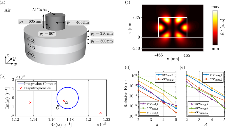
Figure 2: Numerical investigation of the high-$Q$ resonance of a nanophotonic resonator. (a) Nanoresonator on a three-layer substrate. The substrate is infinitely extended in $x$ and $y$ direction. The geometrical parameters $p_{1},p_{2},\dots,p_{5}$ are the reference values from Ref. Koshelev et al. (2020). (b) Calculated eigenfrequency $\tilde{\omega}=(1.17309-0.00296i)\times 10^{15}\,\mathrm{s}^{-1}$ corresponding to the high-$Q$ resonance. The other red crosses shown are the two eigenfrequencies which are closest to $\tilde{\omega}$. The circular integration contour $\tilde{C}$ with the center $\omega_{0}=2\pi c/(1600\,\mathrm{nm})$ and the radius $r_{0}=\omega_{0}\times 10^{-2}$ is used for computing Riesz projections. (c) Electric field intensity $|\tilde{\mathbf{E}}|^{2}$ corresponding to the high-$Q$ resonance. (d) Convergence of the eigenfrequency sensitivities $\partial\tilde{\omega}/\partial p_{i}$ with respect to the polynomial degree $d$ of the FEM ansatz functions. The sensitivities are computed at the parameter reference values given in Fig. 2(a). Relative errors $err_{\mathrm{real},i}=\Bigl{|}\mathrm{Re}\left(\frac{\partial\tilde{\omega}}{\partial p_{i}}(d)-\frac{\partial\tilde{\omega}}{\partial p_{i}}(d_{\mathrm{ref}})\right)/\mathrm{Re}\left(\frac{\partial\tilde{\omega}}{\partial p_{i}}(d_{\mathrm{ref}})\right)\Bigr{|}$, where $d_{\mathrm{ref}}=6$. (e) Relative errors $err_{\mathrm{imag},i}$ for the imaginary parts of the sensitivities; cf. (d).

For the calculation of the contour integrals, a numerical integration with a circular integration contour and a trapezoidal rule is used, which leads to an exponential convergence behavior with respect to the integration points Trefethen and Weideman (2014). At each integration point, we calculate $\mathbf{E}$ and $\partial\mathbf{E}/\partial p_{i}$ by solving Eq. (1) with oblique incident plane waves as source terms. The linear functional $\mathcal{L}(\mathbf{E})$ corresponds to a spatial point evaluation of one component of the electric field, which can be understood as physical observable. Note that, with Eq. (3) and Eq. (4), an eigenfrequency $\tilde{\omega}$ and its sensitivity $\partial\tilde{\omega}/\partial p_{i}$ can be calculated without solving resonance problems $\nabla\times\mu^{-1}\nabla\times\tilde{\mathbf{E}}-\tilde{\omega}^{2}\epsilon\tilde{\mathbf{E}}=0$ directly. Instead, scattering problems, where Eq. (5) can be exploited, are solved. We call the described approach, which combines Riesz projections and direct differentiation (DD), the Riesz projection DD method. Equation (4) and its numerical implementation exploiting Eq. (5) are the main results of this work and represent the difference from previous works on Riesz projections; cf. Ref. Zschiedrich et al. (2018).

Note that the Riesz projection DD method is not limited to the field of nanophotonics, but can be applied to other eigenproblems as well. Maxwell’s equations can be replaced by another partial differential equation, and then instead of the analytical continuation of the electric field $\mathbf{E}$, the analytical continuation of another quantity is evaluated for the contour integration.

III Application

III.1 Eigenfrequency sensitivities of a nanophotonic resonator

We investigate an example from the literature, a dielectric nanoresonator of cylindrical shape placed on a three-layer substrate, where constructive and destructive eigenmode interference has been used to engineer a bound state in the continuum (BIC) Koshelev et al. (2020). The nanoresonator has been designed taking into account various parameters to suppress radiation losses: The radius, the layer thicknesses, and the layer materials have been chosen to obtain a high-$Q$ resonance. The nanoresonator is made of the high-index material aluminum gallium arsenide (AlGaAs) with $20\,\%$ aluminum. A silicon dioxide ($\mathrm{SiO}_{2}$) spacer is placed between the nanoresonator and a film of indium tin oxide (ITO) on a $\mathrm{SiO}_{2}$ substrate. A sketch of the designed system is shown in Fig. 2(a). For this specific configuration, a high-$Q$ resonance with a $Q$-factor of $Q=188\pm 5$ has been experimentally observed, and numerical simulations have resulted in $Q=197$, where the real part of the resonance wavelength is in the telecommunication wavelength regime, close to $1600\,\mathrm{nm}$. The nanophotonic resonator has been exploited as a nanoantenna for nonlinear nanophotonics Koshelev et al. (2020).

In the following simulations, we consider the constant relative permittivities $\epsilon_{\mathrm{r}}=10.81$ and $\epsilon_{\mathrm{r}}=2.084$ for AlGaAs and for $\mathrm{SiO}_{2}$, respectively, which are extracted from experimental data Koshelev et al. (2020); Malitson (1965). For the ITO layer, the Drude model $\epsilon_{\mathrm{r}}(\omega_{0})=\epsilon_{\mathrm{inf}}-\omega^{2}_{\mathrm{p}}/(\omega_{0}^{2}+i\omega_{0}\gamma)$ is chosen, where $\epsilon_{\mathrm{inf}}=3.8813$, $\omega_{\mathrm{p}}=3.0305\times 10^{15}\,\mathrm{s}^{-1}$, and $\gamma=1.2781\times 10^{14}\,\mathrm{s}^{-1}$. This Drude model is obtained by a rational fit Sehmi et al. (2017) to experimental data Koshelev et al. (2020) and describes the material dispersion of the system. We further exploit the rotational symmetry of the geometry. On the one hand, this reduces the computational effort and, on the other hand, the eigenmodes can be easily distinguished by their azimuthal quantum numbers $m$, which correspond to the number of oscillations in the radial and axial directions. When the light sources used for computing Riesz projections are not rotationally symmetric, such as oblique incident plane waves, the source fields can be expanded into Fourier modes in the angular direction. Considering Fourier modes with certain quantum numbers, only the eigenmodes, eigenfrequencies, and corresponding sensitivities associated with these quantum numbers are accessed.

$i$	$\mathrm{Re}(\partial\tilde{\omega}/\partial p_{i})\times 10^{-10}$	$\mathrm{Im}(\partial\tilde{\omega}/\partial p_{i})\times 10^{-10}$
$1$	$-128.750\,(\mathrm{s\,nm})^{-1}\hskip 36.98866pt$	$-0.324\,(\mathrm{s\,nm})^{-1}\hskip 11.38092pt$
$2$	$-84.568\,(\mathrm{s\,nm})^{-1}\hskip 36.98866pt$	$2.660\,(\mathrm{s\,nm})^{-1}\hskip 11.38092pt$
$3$	$-7.192\,(\mathrm{s\,nm})^{-1}\hskip 36.98866pt$	$-1.955\,(\mathrm{s\,nm})^{-1}\hskip 11.38092pt$
$4$	$-0.065\,(\mathrm{s\,nm})^{-1}\hskip 36.98866pt$	$0.208\,(\mathrm{s\,nm})^{-1}\hskip 11.38092pt$
$5$	$15.047\,(\mathrm{s\,deg})^{-1}\hskip 36.98866pt$	$0.039\,(\mathrm{s\,deg})^{-1}\hskip 11.38092pt$

Table 1: Computed eigenfrequency sensitivities. The sensitivities $\partial\tilde{\omega}/\partial p_{i}$ correspond to the high-$Q$ resonance of the nanoresonator shown in Fig. 2(a) and are computed at the shown parameter reference values.

We start with computing a Riesz projection to obtain the eigenfrequency $\tilde{\omega}$ of the high-$Q$ resonance. Figure 2(b) shows the complex frequency plane with the calculated eigenfrequency, $\tilde{\omega}=(1.17309-0.00296i)\times 10^{15}\,\mathrm{s}^{-1}$, and the corresponding circular integration contour $\tilde{C}$ for the computation of the Riesz projection. The center and the radius of the contour are selected based on a-priori knowledge from Ref. Koshelev et al. (2020). Alternatively, without a-priori knowledge, a larger integration contour can be used Betz et al. (2021). The simulations are performed using eight integration points on the contour $\tilde{C}$, where a sufficient accuracy with respect to the integration points is ensured. The computations are based on a FEM mesh consisting of $306$ triangles. To compare the size of the contour with the distances between the eigenfrequencies within the spectrum of the nanoresonator, the two eigenfrequencies which are closest to $\tilde{\omega}$ are also shown. We obtain a $Q$-factor of $Q=198$ for the high-$Q$ resonance, which is in good agreement with the experimental and numerical results from Ref. Koshelev et al. (2020). The corresponding electric field intensity $|\tilde{\mathbf{E}}|^{2}$ is shown in Fig. 2(c). The eigenmode $\tilde{\mathbf{E}}$ has the quantum number $m=0$ and is strongly localized in the vicinity of the nanoresonator.

Next, the eigenfrequency sensitivities $\partial\tilde{\omega}/\partial p_{i}$ with respect to the parameters $p_{1},p_{2},\dots,p_{5}$ sketched in Fig. 2(a) are computed. In order to validate the approach, a convergence study for the polynomial degree $d$ of the FEM ansatz functions is performed. Figures 2(d,e) show the relative errors for the real and imaginary parts, respectively. Exponential convergence can be observed for all sensitivities with increasing $d$. The computed sensitivities for $d=5$ are shown in Tab. 1. Exemplary source code for the Riesz projection DD method and simulation results are presented in Ref. Binkowski et al. (2022).

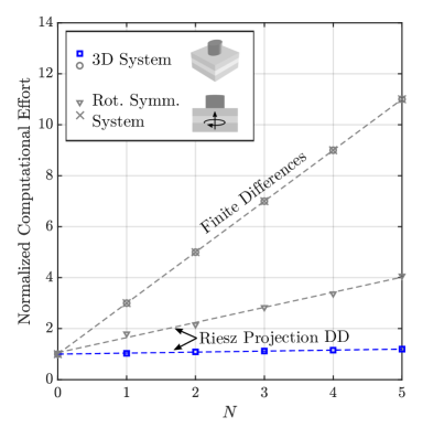
Figure 3: Performance of the Riesz projection DD method. The normalized computational effort over the number $N$ of computed sensitivities $\partial\tilde{\omega}/\partial p_{i}$ with respect to parameters $p_{1},p_{2},\dots,p_{N}$ is shown. The sensitivities are computed at the reference values shown in Fig. 2(a). The computational effort is the total CPU time normalized to the CPU time spent for computing the eigenfrequency $\tilde{\omega}$, which corresponds to $N=0$. The time is measured with JCMsuite using four threads on a machine with a 24-core Intel Xeon Processor running at $3.3\,\mathrm{GHz}$. For all calculations, to ensure high accuracies, eight integration points at the integration contour $\tilde{C}$ depicted in Fig. 2(b) are used. The degree of the FEM ansatz functions is fixed with $d=5$. The mesh of the three-dimensional system consists of $4160$ prisms and the mesh of the rotational symmetric system consists of $306$ triangles.

III.2 Performance benchmark

The computational effort of the numerical realization of the Riesz projection DD method is compared with the computational effort of the finite difference method. We choose the central difference scheme $\partial\tilde{\omega}/\partial p_{i}\approx\left(\tilde{\omega}(p_{i}+\delta p_{i})-\tilde{\omega}(p_{i}-\delta p_{i})\right)/\left(2\delta p_{i}\right)$ for the comparison. Computing central differences is more computationally expensive than computing forward or backward differences. However, more accurate results can be achieved as the error decreases with $(\delta p_{i})^{2}$. To achieve an adequate accuracy, sufficiently small step sizes $\delta p_{i}$ are selected. For example, for the radius of the nanoresonator, we choose $\delta p_{1}=0.1\,\mathrm{nm}$. Note that, also for the finite difference method, we compute the eigenfrequencies by using the contour-integral-based formula in Eq. (3).

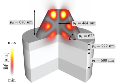
Figure 4: Optimization of a nanophotonic resonator. The optimized nanophotonic resonator with a sketch of the electric field intensity $|\tilde{\mathbf{E}}|^{2}$ corresponding to the high-$Q$ resonance is shown. The high-$Q$ resonance has a $Q$-factor of $Q=292$. The materials of the nanoresonator are the same as for the reference structure in Fig 2(a).

We increase the degrees of freedom of the system shown in Fig 2(a) by deforming the cylindrical nanoresonator to an ellipsoidal nanoresonator. This breaks the rotational symmetry yielding a full three-dimensional system with new parameters, the radius of the nanoresonator in $x$ direction and the radius in $y$ direction. Figure 3 shows, for the three-dimensional implementation and for the rotational symmetric implementation, the normalized computational effort for different numbers of computed sensitivities. We compute the eigenfrequency $\tilde{\omega}$ and then we add the sensitivities, starting with $\partial\tilde{\omega}/\partial p_{1}$, one after the other. It can be observed that the Riesz projection DD method requires less computational effort than the finite difference method, for any number of computed sensitivities, i.e., for all $N\geq 1$. In the case of using finite differences, the computational effort has a slope of about $200\,\%$ because for each sensitivity two additional problems with typically the same dimension as the unperturbed problem have to be solved. In the three-dimensional case, a linear regression for the computational effort gives a slope of about $4\,\%$ for the Riesz projection DD method. The computational effort needed for the $LU$-decomposition is significant compared to the matrix assembly and to the other solution steps, so the possibility of exploiting Eq. (5) gives a great benefit for the Riesz projection DD method. For $N=5$, the CPU time required to solve the linear system of equations, which includes the $LU$-decomposition, takes $81\,\%$ of the accumulated CPU time. In the rotational symmetric case, the time for solving the linear system is negligible. However, the trend is the same for the three-dimensional and for the computationally cheaper rotational symmetric case: The advantage of using Riesz projections significantly increases with an increasing number of computed sensitivities.

Note that contour integral methods are well suited for parallelization because the scattering problems can be solved in parallel on the integration contour. However, as total CPU times are considered for Fig. 3, this is not reflected by the time measurements.

III.3 $Q$-factor optimization

The Riesz projection DD method is applied to further optimize the $Q$-factor of the high-$Q$ resonance of the nanophotonic resonator from Ref. Koshelev et al. (2020) shown in Fig. 2(a). A rotational symmetric nanoresonator is considered because simulations show that an ellipsoidal shape does not lead to a significant increase of the $Q$-factor. We use a Bayesian optimization algorithm Pelikan et al. (1999) with the incorporation of sensitivity information. This global optimization algorithm is well suited for problems with computationally expensive objective functions and benchmarks show that providing sensitivities can significantly reduce computational effort Schneider et al. (2019). However, other optimization approaches could be used as well.

For the optimization, we choose the parameter ranges $435\,\mathrm{nm}\leq p_{1}\leq 495\,\mathrm{nm}$, $575\,\mathrm{nm}\leq p_{2}\leq 695\,\mathrm{nm}$, $150\,\mathrm{nm}\leq p_{3}\leq 550\,\mathrm{nm}$, $100\,\mathrm{nm}\leq p_{4}\leq 500\,\mathrm{nm}$, and $60^{\circ}\leq p_{5}\leq 90^{\circ}$. To ensure that the optimized nanoresonator can also be used as nanoantenna in the telecommunication wavelength regime, like the original system, we add the constraint that the optimized eigenfrequency must lie in the circular contour with the center $\omega_{0}=2\pi c/(1600\,\mathrm{nm})$ and the radius $r_{0}=4\times 10^{13}\,\mathrm{s}^{-1}$. In each optimization step, the Riesz projection DD method is used to compute the eigenfrequency with a quantum number of $m=0$ lying inside the contour and to calculate the corresponding sensitivities.

A nanoresonator with a $Q$-factor of $Q=292$ is obtained after $61$ iterations of the optimizer yielding an increase of about $47.5\,\%$ over the original resonator. More iterations yield only a negligible increase of the $Q$-factor. The optimized nanoresonator with a sketch of the electric field intensity of its high-$Q$ resonance and the values for all underlying parameters are shown in Fig. 4. The corresponding eigenfrequency is given by $\tilde{\omega}_{\mathrm{opt}}=(1.176897-0.002015i)\times 10^{15}\,\mathrm{s}^{-1}$. Note that, in the optimization domain, the average sensitivity of the $Q$-factor with respect to the ITO layer thickness $p_{4}$ is negligible.

IV Conclusions

An approach for computing eigenfrequency sensitivities of resonance problems was presented. The numerical realization of the Riesz projection DD method relies on computing scattering solutions and their sensitivities by solving Maxwell’s equations with a source term, i.e., solving linear systems of equations. This enables direct differentiation for the efficient calculation of eigenfrequency sensitivities. Although sensitivities of resonances are computed, no eigenproblems have to be solved directly. The performance of the approach was demonstrated by a comparison with the finite difference method. The Riesz projection DD method was incorporated into a gradient-based optimization algorithm to maximize the $Q$-factor of a nanophotonic resonator.

The savings in computational effort are particularly significant for optimization with respect to several parameters, which is a common task in nanophotonics. Therefore, we expect the approach to prove especially useful when many sensitivities are to be calculated. The Riesz projection DD method can not only be applied to problems in nanophotonics, but to any resonance problem.

Data and code availability

All relevant data generated or analysed during this study are included in this work. Tabulated data files and source code for performing the numerical experiments can be found in Ref. Binkowski et al. (2022).

References

- Novotny and van Hulst (2011) L. Novotny and N. van Hulst, Nat. Photonics 5, 83 (2011).
- Kuznetsov et al. (2016) A. I. Kuznetsov, A. E. Miroshnichenko, M. L. Brongersma, Y. S. Kivshar, and B. Luk’yanchuk, Science 354, aag2472 (2016).
- Senellart et al. (2017) P. Senellart, G. Solomon, and A. White, Nat. Nanotechnol. 12, 1026 (2017).
- Anker et al. (2008) J. N. Anker, W. P. Hall, O. Lyandres, N. C. Shah, J. Zhao, and R. P. Van Duyne, Nat. Mater. 7, 442 (2008).
- Ma and Oulton (2019) R.-M. Ma and R. F. Oulton, Nat. Nanotechnol. 14, 12 (2019).
- Ma et al. (2016) X.-C. Ma, Y. Dai, L. Yu, and B.-B. Huang, Light Sci. Appl. 5, e16017 (2016).
- Zhang et al. (2018) Y. Zhang, S. He, W. Guo, Y. Hu, J. Huang, J. R. Mulcahy, and W. D. Wei, Chem. Rev. 118, 2927 (2018).
- Lalanne et al. (2018) P. Lalanne, W. Yan, K. Vynck, C. Sauvan, and J.-P. Hugonin, Laser Photonics Rev. 12, 1700113 (2018).
- Wu et al. (2021) T. Wu, M. Gurioli, and P. Lalanne, ACS Photonics 8, 1522 (2021).
- West et al. (2010) P. West, S. Ishii, G. Naik, N. Emani, V. Shalaev, and A. Boltasseva, Laser Photonics Rev. 4, 795 (2010).
- Wang et al. (2021) B. Wang, P. Yu, W. Wang, X. Zhang, H.-C. Kuo, H. Xu, and Z. M. Wang, Adv. Opt. Mater. 9, 2001520 (2021).
- Lalanne et al. (2019) P. Lalanne, W. Yan, A. Gras, C. Sauvan, J.-P. Hugonin, M. Besbes, G. Demésy, M. D. Truong, B. Gralak, F. Zolla, A. Nicolet, F. Binkowski, L. Zschiedrich, S. Burger, J. Zimmerling, R. Remis, P. Urbach, H. T. Liu, and T. Weiss, J. Opt. Soc. Am. A 36, 686 (2019).
- Bindel and Hood (2013) D. Bindel and A. Hood, SIAM J. Matrix Anal. Appl. 34, 1728 (2013).
- Güttel and Tisseur (2017) S. Güttel and F. Tisseur, Acta Numer. 26, 1 (2017).
- Jensen and Sigmund (2011) J. Jensen and O. Sigmund, Laser Photonics Rev. 5, 308 (2011).
- Bouhlel et al. (2019) M. A. Bouhlel, J. T. Hwang, N. Bartoli, R. Lafage, J. Morlier, and J. R. Martins, Adv. Eng. Softw. 135, 102662 (2019).
- Cacuci et al. (2005) D. G. Cacuci, M. Ionescu-Bujor, and I. M. Navon, Sensitivity and Uncertainty Analysis, Volume II: Applications to Large-Scale Systems, 1st ed. (CRC Press, 2005).
- Kato (1995) T. Kato, Perturbation Theory for Linear Operators, 2nd ed. (Springer-Verlag Berlin Heidelberg, 1995).
- Sakurai and Napolitano (2020) J. J. Sakurai and J. Napolitano, Modern Quantum Mechanics, 3rd ed. (Cambridge University Press, 2020).
- Burschäpers et al. (2011) N. Burschäpers, S. Fiege, R. Schuhmann, and A. Walther, Adv. Radio Sci. 9, 85 (2011).
- Swillam et al. (2008) M. A. Swillam, M. H. Bakr, X. Li, and M. J. Deen, Opt. Commun. 281, 4459 (2008).
- Yan et al. (2020) W. Yan, P. Lalanne, and M. Qiu, Phys. Rev. Lett. 125, 013901 (2020).
- Alam and Safique Ahmad (2019) R. Alam and S. Safique Ahmad, SIAM J. Matrix Anal. Appl. 40, 672 (2019).
- Binkowski et al. (2020) F. Binkowski, L. Zschiedrich, and S. Burger, J. Comput. Phys. 419, 109678 (2020).
- Betz et al. (2021) F. Betz, F. Binkowski, and S. Burger, SoftwareX 15, 100763 (2021).
- Zschiedrich et al. (2018) L. Zschiedrich, F. Binkowski, N. Nikolay, O. Benson, G. Kewes, and S. Burger, Phys. Rev. A 98, 043806 (2018).
- Pomplun et al. (2007) J. Pomplun, S. Burger, L. Zschiedrich, and F. Schmidt, Phys. Status Solidi B 244, 3419 (2007).
- Hohenester and Trügler (2012) U. Hohenester and A. Trügler, Comput. Phys. Commun. 183, 370 (2012).
- Nikolova et al. (2004) N. Nikolova, J. Bandler, and M. Bakr, IEEE Trans. Microw. Theory Techn. 52, 403 (2004).
- Burger et al. (2013) S. Burger, L. Zschiedrich, J. Pomplun, F. Schmidt, and B. Bodermann, Proc. SPIE 8681, 380 (2013).
- Koshelev et al. (2020) K. Koshelev, S. Kruk, E. Melik-Gaykazyan, J.-H. Choi, A. Bogdanov, H.-G. Park, and Y. Kivshar, Science 367, 288 (2020).
- Trefethen and Weideman (2014) L. Trefethen and J. Weideman, SIAM Rev. 56, 385 (2014).
- Malitson (1965) I. H. Malitson, J. Opt. Soc. Am. 55, 1205 (1965).
- Sehmi et al. (2017) H. S. Sehmi, W. Langbein, and E. A. Muljarov, Phys. Rev. B 95, 115444 (2017).
- Binkowski et al. (2022) F. Binkowski, F. Betz, M. Hammerschmidt, P.-I. Schneider, L. Zschiedrich, and S. Burger, “Source code and simulation results for Computation of eigenfrequency sensitivities using Riesz projections for efficient optimization of nanophotonic resonators,” Zenodo (2022), https://doi.org/10.5281/zenodo.6614951.
- Pelikan et al. (1999) M. Pelikan, D. E. Goldberg, and E. Cantú-Paz, GECCO’99: Proc. Gen. Ev. Comp. Conf. 1, 525 (1999).
- Schneider et al. (2019) P.-I. Schneider, X. Garcia Santiago, V. Soltwisch, M. Hammerschmidt, S. Burger, and C. Rockstuhl, ACS Photonics 6, 2726 (2019).