Stochastic Galerkin finite element method for nonlinear elasticity and application to reinforced concrete members

Abstract

We develop a stochastic Galerkin finite element method for nonlinear elasticity and apply it to reinforced concrete members with random material properties. The strategy is based on the modified Newton-Raphson method, which consists of an incremental loading process and a linearization scheme applied at each load increment. We consider that the material properties are given by a stochastic expansion in the so-called generalized polynomial chaos (gPC) framework. We search the gPC expansion of the displacement, which is then used to update the gPC expansions of the stress, strain and internal forces. The proposed method is applied to a reinforced concrete beam with uncertain initial concrete modulus of elasticity and a shear wall with uncertain maximum compressive stress of concrete, and the results are compared to those of stochastic collocation and Monte Carlo methods. Since the systems of equations obtained in the linearization scheme using the stochastic Galerkin method are very large, and there are typically many load increments, we also studied iterative solution using preconditioned conjugate gradients. The efficiency of the proposed method is illustrated by a set of numerical experiments.

1 Introduction

Reinforced concrete is one of the most popular materials in construction. Therefore predicting the behavior of reinforced concrete members and structures is very important. However, development of the analytical models for reinforced concrete is complicated by several factors. Reinforced concrete is composed of concrete and steel, which are two materials with different nonlinear properties. In particular, concrete exhibits a nonlinear softening behavior in compression and a linear brittle behavior in tension, and its combination with steel makes the behavior of reinforced concrete members even more complex. The computational analysis is commonly performed using the finite element method. To this end, considerable number of constitutive models was developed to characterize the nonlinear behavior and stress strain relationship of concrete and its reinforcement. In traditional approaches, the physical characteristics of reinforced concrete are considered to be known and the problem is deterministic. However, in practice the structural properties of these materials typically show variability, which usually result from the manufacturing process, natural variability in microstructure and possibly also from aging. Additional factors, such as uncertainty in external loading, may also contribute to the uncertainty in the predicted response. Propagation and quantification of uncertainty using numerical simulations for risk and reliability analysis as well as design of reinforced concrete members and structures is therefore a critical task of engineering research.

The most widely applied technique for approximating quantities of interest for problems with random inputs is Monte Carlo method [1, 2]. It is simple to implement, but the main weakness is relatively slow convergence. Another important class is given by perturbation methods [3, 4], which are however limited to problems with small variability of uncertainty. An alternative that gained a significant attention in the last two decades is the stochastic finite element method [5, 6]. The assumption is that a parametric uncertainty is described in terms of polynomials of random variables using the so-called generalized polynomial chaos (gPC) framework [7] and one searches for gPC expansions of solutions. There are two main approaches: stochastic collocation method (SC), which is based on sampling that translates the problem into a set of uncoupled deterministic problems cf, e.g., [8, 9, 10], and stochastic Galerkin method (SG), which by means of the Galerkin projection couples the physical and probabilistic degrees of freedom into a single large system of equations cf. also, e.g., [11, 10, 12]. Both approaches have been used in various applications in structural engineering [13], see also [14]. Due to the large size of the linear systems arising in the stochastic Galerkin method, iterative solution may be the preferred choice since use of direct solvers may be prohibitive. When the finite element discretization of the underlying deterministic problem leads to a symmetric, positive definite matrix, the global stochastic Galerkin matrix is typically also positive definite [15]. Then the corresponding linear system can be solved using the conjugate gradient method, and its preconditioning is often a vital component enabling to speed up convergence and reduce computational time. The most simple, yet often surprisingly effective is the mean-based, block-diagonal preconditioner proposed by Pellissetti and Ghanem [16] and analyzed by Powell and Elman [17]. Other preconditioners use either more terms from the gPC expansion of the coefficient matrix or imitate the structure of the stochastic Galerkin matrix [18, 19, 20, 21], or use advanced solvers as their components such as domain decomposition [22, 23, 24, 25] or multigrid [26, 27, 28], see also [29, 30, 31]. One of the most recent advancements includes the truncation preconditioners [21, 32, 33], which we also use in our numerical experiments. We note that a similar study to ours was recently presented by [34], but here we focus on a more complex nonlinear model that includes a crack development, and we also study efficient solution of the linear systems obtained by use of the stochastic Galerkin method.

In this paper, we develop the stochastic Galerkin finite element method for propagation of uncertainty in a nonlinear elasticity model and apply to reinforced concrete members with random material properties. In particular, we consider uncertainty in the modulus of elasticity, which (nonlinearly) depends on the strain (deformation). We describe a linearization scheme based on the modified Newton-Raphson method formulated in the context of the stochastic Galerkin framework. The method consists of an incremental loading process and a linearization scheme applied at each load increment. The tangent stiffness matrix is updated after each load increment, and each increment is further subdivided into a number of steps. In each such step, the structural response is translated into the vector of internal forces, which then modifies the right-hand sides of the linearized problems. The whole process continues until the full load is applied and the displacement increment vector is smaller than a given tolerance. We consider that the material properties (stiffness) are given by a stochastic expansion, in the so-called generalized polynomial chaos (gPC) framework. We search the gPC expansion of the displacement, which is then used to update the gPC expansions of the stress, strain and internal forces between each step of a load increment. Stochastic tangent stiffness matrices are updated at the first step of each load increment. The method is applied to a reinforced concrete beam with uncertain initial concrete modulus of elasticity and a shear wall with uncertain maximum compressive stress of concrete under deterministic concentrated loading and the results are compared to that of Monte Carlo and stochastic collocation methods. Next, since the size of the linear systems in the stochastic Galerkin method is usually large, we also study iterative solution using preconditioned conjugate gradients.

The paper is organized as follows. In Section 2 we recall the general implementation of deterministic nonlinear FEM, in Section 3.1 we formulate the stochastic Galerkin finite element method that accounts for a nonlinearity in the material properties, in Section 3.2 we discuss the sampling methods (Monte Carlo and stochastic collocation), in Section 3.3 we present the application of the proposed procedure to a simply supported beam and in Section 3.4 to a shear wall with random material properties, In section 4 we study iterative solution of the linear systems arising in the stochastic Galerkin method, and finally in Section 5 we summarize and conclude our work.

2 Deterministic nonlinear model

We recall the deterministic nonlinear finite element formulation for reinforced concrete members based on [35]. We consider that the response is mainly caused by nonlinearity in stress-strain relations, due to cracking of concrete and due to yielding of steel reinforcement. In general, structure of concrete is very complex because it is a composite made up of hydrated cement, sand, and coarse aggregates. In addition, it contains numerous flaws and micro-cracks, and the rapid propagation of micro-cracks under applied loads contributes to the nonlinear properties of concrete as well. Numerical simulation of reinforced concrete members requires realistic stress-strain relations of the plain concrete as an input. Such formulations are thus nonlinear and rely on a number of experimentally determined material constants.

For the concrete, we will use the representation by the nonlinear elasticity model based on the limiting tensile strain failure criterion that covers the pre-peak and post-peak regimes from [36]. This model is expressed in terms of tangent stiffness formulation. It is assumed that stresses in the principal directions can be calculated independently of each other, based on uniaxial stress-strain relationships. The biaxial effect was assumed to be due to the interaction of the two principal directions through the Poisson’s ratio effect. Therefore, the concept of equivalent uniaxial strain should be introduced in order to separate the Poisson effect from the cumulative strain [37]. In addition, equivalent uniaxial strain can make a contribution to keep track of the degradation of stiffness and strength of plain concrete and to allow actual biaxial stress-strain curves to be derived from uniaxial curves. The uniaxial curves selected for compressive loading in this study are based on an equation suggested by the FIB model code [38] as

$$\frac{\sigma_{c}}{f_{cm}}=-\frac{k\eta-\eta^{2}}{1+(k-2)\eta}\ \quad\text{for}\ |\epsilon_{c}|<|\epsilon_{c,lim}|,$$ (1)

where $\sigma_{c}$ is the compressive stress in MPa, $f_{cm}=\acute{f}_{c}+8$ is the actual compressive strength of concrete at an age of 28 days in MPa (here $\acute{f}_{c}$ is the specific compressive strength of concrete in MPa), $k=E_{ci}/E_{c1}$ is the plasticity number (here $E_{ci}$ is the tangent modulus of elasticity in MPa, and $E_{c1}$ is the secant modulus from the origin to the peak compressive stress), and $\eta=\epsilon_{c}/\epsilon_{c1}$ (here $\epsilon_{c}$ is the compressive strain and $\epsilon_{c1}$ is the strain at the maximum compressive stress). Then, a complete stress-strain curve of concrete in uniaxial tension can be treated based on an equation suggested by FIB model code [38] as

$$\sigma_{ct}=\begin{cases}E_{ci}\,\epsilon_{ct}&\text{for}\ \sigma_{ct}\leq 0.9f_{ctm},\\ f_{ctm}\left(1-0.1\frac{0.00015-\epsilon_{ct}}{0.00015-0.9f_{ctm}/E_{ci}}\right)&\text{for}\ 0.9f_{ctm}<\sigma_{ct}\leq f_{ctm}\end{cases}$$ (2)

where $\sigma_{ct}$ is the tensile stress in MPa, $E_{ci}$ is the tangent modulus of elasticity in MPa, $\epsilon_{ct}$ is the tensile strain, and $f_{ctm}$ is the tensile strength in MPa.

In contrast with concrete, the mechanical properties of steel reinforcement are well known. The reinforcing steel bars are assumed to be only transmitting axial compressive or tensile forces. Thus, an uniaxial stress-strain relationship is sufficient. Under monotonic loading, it is generally assumed that the steel behavior is identical in tension and compression. In this study, a bilinear stress-strain relation suggested by FIB model code [38] is used as

$$\sigma_{s}=\begin{cases}E_{s}\,\epsilon_{s}&\text{for}\ \epsilon_{s}<\epsilon_{sy},\\ f_{y}+E_{sh}\,(\epsilon_{s}-\epsilon_{sy})&\text{for}\ \epsilon_{sy}\leq\epsilon_{s}\leq\epsilon_{su}\end{cases}$$ (3)

where $\sigma_{s}$ is the stress, $E_{s}$ is the initial modulus of elasticity, $\epsilon_{s}$ is the strain, $\epsilon_{sy}$ is the yielding strain, $f_{y}$ is the yielding stress, $E_{sh}$ is the modulus of strain hardening and $\epsilon_{su}$ is the ultimate strain.

The phenomenon of concrete cracking is extremely important in the behavior of reinforced concrete structures. The maximum stress and strain theories are frequently used to determine whether tensile cracking has occurred in the concrete [39]. If the maximum principal stress or strain in a point of the structure reaches the uniaxial tensile strength or tensile strain limit, cracking is assumed to form perpendicular to the direction of the maximum tensile stress or strain. The stress in that direction is subsequently reduced to zero. The limiting tensile stress value which causes the crack is not a well-defined quantity. For specimens cast from the same concrete, the flexural tensile strength determined from a modulus of rupture test is higher than the tensile strength of a split cylinder, which is in turn higher than the tensile strength obtained from a direct tension test. Furthermore, for each type of test there is significant scatter in the results. For concrete structures subjected to rapid loading, the maximum strain criterion is more realistic, since uniaxial dynamic tensile tests indicate that an almost constant failure strain is observed irrespective of the strain rate or loading rate [40]. The limiting tensile strain criterion has been employed with success to represent the tensile cracking of concrete under static loading [41]. In this study, we use a smeared crack approach proposed by [42]. It is based on the limiting tensile strain criterion, and it allows the concrete to crack in one or two directions. In fact, it offers complete generality in possible crack direction. This representation is also popular since it allows for automatic generation of cracks without redefinition of the finite element topology. Instead of redefining the finite element mesh and nodal connectivities, cracking is accounted for by modifying the material properties within elements. After the crack has occurred in an element, the concrete becomes an orthotropic material with one of the material axes being oriented along the direction of cracking, and the elasticity modulus in the direction perpendicular to the cracking plane is reduced to zero. Next, a reduced shear modulus is assumed on the cracked plane to account for aggregate interlocking. Shear transmission due to aggregate interlock can be simply accounted for in the smeared crack model by the introduction of a reduced value of concrete shear modulus. In this study, we used a proposed model by [43]. The tension stiffening effect of cracked concrete is also incorporated into this model by including a descending branch in the stress-strain curve of concrete under tension. In this study, we use a linear descending branch in the stress-strain curve of concrete under tension for considering tension stiffening effect, and other nonlinear effects such as crushing of concrete in compression and yielding or strain hardening of steel reinforcement are also taken into account, as suggested by FIB model code [38].

We combine the constitutive equations with the compatibility and equilibrium equations, compute the weak form of the equilibrium equations and replace the displacement field by its finite element approximation. This yields a discrete nonlinear equilibrium system, which may be formally written as

$$\mathcal{K}(u)=f,$$ (4)

where $\mathcal{K}(u)$ is the nonlinear operator that depends on the model parameters but also on the displacement vector $u$, and $f$ is the vector of external load. We now formulate the modified Newton-Raphson method to solve system (4). The method is based on linearization of the nonlinear operator and incremental application of the external load. The tangent stiffness matrix is updated after each load increment, and the system is assumed linear during a load increment. Each load increment is further subdivided into several steps, during which only the right-hand side is updated. The system of linearized equations at step$~{}i$ of the $n$th load increment can be written as

$$K^{n}\Delta u^{n,i}=f^{n}-g\left(u^{n,i-1}\right),$$ (5)

where $K^{n}$ is the corresponding tangent stiffness matrix of size $n_{x}\times n_{x}$, $\Delta u^{n,i}$ is the increment of displacement vector, $f^{n}$ is the external load vector and $g\left(u^{n,i-1}\right)$ is the internal force vector at $(i-1)$th step of the $n$th load increment. The matrix $K^{n}$ is obtained by assembly of finite element matrices. The matrix of the $e$th element at the $n$th load increment is computed as

$$K_{e}^{n}=\int_{v_{e}}B_{e}^{T}D_{e}^{n}B_{e}\,dv_{e},$$ (6)

where $B_{e}$ is the element shape function derivative matrix and $D_{e}^{n}$ is the element stress-strain matrix computed as

$$D_{e}^{n}=D_{c,e}^{n}+D_{s,e}^{n},$$ (7)

where $D_{c,e}^{n}$ and $D_{s,e}^{n}$ are concrete and steel rebar stress-strain matrices, respectively. For the first load increment, the concrete stress-strain matrix is computed as

$$D_{c,e}^{1}=\left[\begin{array}[c]{ccc}\frac{E_{ci}}{1-\nu_{c}^{2}}&\frac{E_{ci}\nu_{c}}{1-\nu_{c}^{2}}&0\\ \frac{E_{ci}\nu_{c}}{1-\nu_{c}^{2}}&\frac{E_{ci}}{1-\nu_{c}^{2}}&0\\ 0&0&\frac{E_{ci}}{2(1+\nu_{c})}\end{array}\right],$$ (8)

where $E_{ci}$ is the initial concrete modulus of elasticity and $\nu_{c}$ is the Poisson coefficient of concrete. For the first load increment, the steel rebar stress-strain matrix is computed as

$$D_{s,e}^{1}=E_{si}\left[\begin{array}[c]{ccc}\rho_{x}&0&0\\ 0&\rho_{y}&0\\ 0&0&0\end{array}\right],$$ (9)

where $E_{si}$ is the initial steel rebar modulus of elasticity and $\rho_{x}$ and $\rho_{y}$ are the steel rebar percentages in $x$ and $y$ directions, respectively. For other load increments, $D_{c,e}^{n}$ and $D_{s,e}^{n}$ are computed using the material constitutive models and the corresponding stress level [35]. Applying numerical integration to eq. (6), we get

$$K_{e}^{n}=\sum_{q_{1}=1}^{m_{1}}\sum_{q_{2}=1}^{m_{2}}\omega_{q_{1}}\omega_{q_{2}}\left[B_{e}(\zeta_{q_{1}},\eta_{q_{2}})\right]^{T}D_{e}^{n}\,B_{e}(\zeta_{q_{1}},\eta_{q_{2}})\det J(\zeta_{q_{1}},\eta_{q_{2}})\,t,$$ (10)

where $m_{1}$, $m_{2}$ are the numbers of quadrature points $\zeta_{q_{1}},$ $\eta_{q_{2}}$ with weights $\omega_{q1}$, $\omega_{q2}$, respectively, $\det J(\zeta_{q1},\eta_{q2})$ is the determinant of the Jacobian matrix, and $t$ is the thickness of the element. The internal force vector$~{}g_{e}(u^{n,i-1})$ is computed for each element in eq. (5) as

$$g_{e}(u^{n,i-1})=\int_{v_{e}}B_{e}^{T}\sigma_{e}^{n,i-1}\,dv_{e},$$ (11)

where $\sigma_{e}^{n,i-1}$ is the stress vector for the $e$th element. Applying numerical integration to eq. (11), we get

$$g_{e}(u^{n,i-1})=\sum_{q_{1}=1}^{m_{1}}\sum_{q_{2}=1}^{m_{2}}\omega_{q_{1}}\omega_{q_{2}}[B_{e}(\zeta_{q_{1}},\eta_{q_{2}})]^{T}\sigma_{e}^{n,i-1}\det J(\zeta_{q_{1}},\eta_{q_{2}})\,t.$$ (12)

The stress vector $\sigma_{e}^{n,i-1}$ is computed as

$$\sigma_{e}^{n,i-1}=\sigma_{e}^{n,i-2}+\Delta\sigma_{e}^{n,i-1},$$ (13)

where $\Delta\sigma_{e}^{n,i-1}$ is the stress vector increment

$$\Delta\sigma_{e}^{n,i-1}=D_{e}^{n}\,\Delta\epsilon_{e}^{n,i-1},$$ (14)

and $\Delta\epsilon_{e}^{n,i-1}$ is the strain vector increment

$$\Delta\epsilon_{e}^{n,i-1}=B_{e}\,\Delta u_{e}^{n,i-1}.$$ (15)

Above, $\Delta u_{e}^{n,i-1}$ is the displacement increment at step $i-1$ of the $n$th load increment for the $e$th element. At the first step of the first load increment, the deformation vector $u^{1,0}=0$, and so the internal force vector $g(u^{n,i-1})=0$. After eq. (5) is solved for the displacement increment$~{}\Delta u^{n,i}$, a new approximate solution is obtained as

$$u^{n,i}=u^{n,i-1}+\Delta u^{n,i}.$$ (16)

This process continues until the displacement increment vector is smaller than a given tolerance.

3 Stochastic finite element method

3.1 The stochastic Galerkin method

We assume that the uncertainty is induced in the model by a vector$~{}\xi$ of independent, identically distributed (i.i.d.) random variables$~{}\xi_{i}$, $i=1,\dots,m_{\xi}$. Specifically, we let the uncertainty enter the model through some of the parameters, more details are given in Section 3.3. Then, the nonlinear system (4) becomes stochastic, and in this study we use the stochastic Galerkin finite element framework to extend the Newton-Raphson method from Section 2 to this case. This framework entails use of a space spanned by a set of multivariate polynomials $\left\{\psi_{\ell}\left(\xi\right)\right\}_{\ell=1}^{n_{\xi}}$, which is known in the literature as a generalized polynomial chaos (gPC) basis [44, 45]. The polynomials are orthonormal with respect to the density function associated with the distribution of$~{}\xi$, and we will in particular assume that

$$\psi_{1}=1,\quad\text{and}\quad\mathbb{E}\left[\psi_{k}\psi_{\ell}\right]=\langle\psi_{k}\psi_{\ell}\rangle=\delta_{k\ell},$$ (17)

where $\mathbb{E}$ is the mathematical expectation, and$~{}\delta_{k\ell}$ denotes the Kronecker delta function.

Suppose we are given a stochastic expansion of the tangent stiffness matrix at the $n$th load increment as

$$K(\xi)^{n}=\sum_{\ell=1}^{n_{K}}K_{\ell}^{n}\,\psi_{\ell}(\xi),$$ (18)

where $K_{\ell}^{n}$ is for each $\ell$ a (deterministic) matrix of size $n_{x}\times n_{x}$. Let us further suppose that the external load vector at the$~{}n$th load increment$~{}f(\xi)^{n}$ and the internal force vector at the $(i-1)$th step of $n$th load increment$~{}g(\xi)^{n,i-1}$ are also given as stochastic expansions

$$f(\xi)^{n} =\sum_{m=1}^{n_{\xi}}f_{m}^{n}\,\psi_{m}(\xi),$$ (19)

$$g(\xi)^{n,i-1} =\sum_{m=1}^{n_{\xi}}g_{m}^{n,i-1}\,\psi_{m}(\xi),$$ (20)

where both $f_{m}^{n}$ and $g_{m}^{n,i-1}$ are vectors of length $n_{x}$ for all$~{}m$. Forming the stochastic counterpart of system (5), we will search for the increment of the displacement vector at the $i$th step of the $n$th load increment in the form

$$\Delta u(\xi)^{n,i}=\sum_{k=1}^{n_{\xi}}\Delta u_{k}^{n,i}\,\psi_{k}(\xi).$$ (21)

Specifically, substituting expansions (18)–(21) into equation (5) and performing a stochastic Galerkin projection, i.e., by orthogonalizing the residual to the gPC basis $\{\psi_{m}\}_{m=1}^{n_{\xi}}$, yields a system of linear deterministic equations

$$\mathbf{K}^{n}\Delta\mathbf{u}^{n,i}=\mathbf{f}^{n}-\mathbf{g}^{n,i-1},\qquad\mathbf{K}^{n}\in\mathbb{R}^{n_{x}n_{\xi}\times n_{x}n_{\xi}}\quad\Delta\mathbf{u}^{n,i},\mathbf{f}^{n},\mathbf{g}^{n,i-1}\in\mathbb{R}^{n_{x}n_{\xi}}.$$ (22)

Denoting $c_{\ell km}=\langle\psi_{\ell}\psi_{k}\psi_{m}\rangle$, the stochastic Galerkin matrix$~{}\mathbf{K}^{n}$ can be written as

$$\mathbf{K}^{n}=\left[\begin{array}[c]{ccc}K_{(1,1)}^{n}&\cdots&K_{({n}_{\xi},1)}^{n}\\ \vdots&\ddots&\vdots\\ K_{(1,{n}_{\xi})}^{n}&\cdots&K_{({n}_{\xi},{n}_{\xi})}^{n}\end{array}\right],\qquad\text{with }{K}_{(k,m)}^{n}=\sum_{\ell=1}^{n_{K}}c_{\ell km}\,{K}_{\ell}^{n},$$ (23)

and the vectors in (22) are concatenations of$~{}n_{\xi}$ subvectors of size$~{}n_{x}$, cf. (19)–(21), as

$$\Delta\mathbf{u}^{n,i}=\left[\begin{array}[c]{c}\Delta u_{1}^{n,i}\\ \vdots\\ \Delta u_{n_{\xi}}^{n,i}\end{array}\right],\qquad\mathbf{f}^{n}=\left[\begin{array}[c]{c}f_{1}^{n}\\ \vdots\\ f_{n_{\xi}}^{n}\end{array}\right],\quad\mathbf{g}^{n,i-1}=\left[\begin{array}[c]{c}g_{1}^{n,i-1}\\ \vdots\\ g_{n_{\xi}}^{n,i-1}\end{array}\right].$$ (24)

For the first step of the first load increment $\mathbf{g}^{1,0}=0$ since $u^{1,0}(\xi)=0$. After solving equation (22), the approximate solution is updated as

$$\mathbf{u}^{n,i}=\mathbf{u}^{n,i-1}+\Delta\mathbf{u}^{n,i}.$$ (25)

For the next steps, the gPC expansion of internal load vector$~{}g^{n,i-1}$ is computed using numerical integration as

$$g_{m}^{n,i-1}=\left\langle g(\xi)^{n,i-1}\,\psi_{m}\right\rangle=\sum_{q=1}^{n_{q}}g(\xi^{(q)})^{n,i-1}\,\psi_{m}(\xi^{(q)})\,\omega^{(q)},$$ (26)

where $\xi^{(q)}$ are quadrature points, $\omega^{(q)}$ are quadrature weights, $n_{q}$ is the number of quadrature points and $g(\xi^{(q)})^{n,i-1}$ is a realization of expansion (20) at $\xi^{(q)}$, which is obtained by assembly of finite element internal load vectors, cf. (12),

$$g(\xi^{(q)})_{e}^{n,i-1}=\sum_{q_{1}=1}^{m_{1}}\sum_{q_{2}=1}^{m_{2}}\omega_{q_{1}}\omega_{q_{2}}[B(\zeta_{q_{1}},\eta_{q_{2}})]^{T}\sigma(\xi^{(q)})_{e}^{n,i-1}\det J(\zeta_{q_{1}},\eta_{q_{2}})\,t.$$ (27)

The realizations of the element internal load vectors in (27) depend on the realizations of the stress vector  $\sigma(\xi^{(q)})_{e}^{n,i-1}$, which in turn depend on the realizations of the stress and strain increments and are computed from the realizations of the displacement increment $\Delta u(\xi^{(q)})_{e}^{n,i-1}$ in the same way as the calculations in (13)–(15).

The terms in expansion of the tangent stiffness matrix (18) are also obtained using numerical integration as

$$K_{j}^{n}=\left\langle K(\xi)^{n}\,\psi_{j}(\xi)\right\rangle=\sum_{q=1}^{n_{q}}K(\xi^{(q)})^{n}\,\psi_{j}(\xi^{(q)})\,\omega^{(q)},$$ (28)

where the realizations of $K(\xi^{(q)})^{n}$ are computed using realizations of the model parameters, with more details given in Section 3.3, and using the realizations of the displacement vector $u(\xi^{(q)})^{n,0}$ from its gPC expansion. This process is repeated until the $\Delta u^{n,i}$ is smaller than a given tolerance. Statistics of the solution, such as mean, standard deviation and probability density function, can be estimated in post-processing phase by sampling the gPC expansions.

3.2 Sampling methods

In numerical experiments described in Section 3.3, we compare results from stochastic Galerkin method to those obtained using two sampling methods: Monte Carlo and stochastic collocation. The sampling entails solving of a number of mutually independent deterministic problems. In the Monte Carlo method, the sample points $\xi^{(q)}$, $q=1,...,n_{MC}$, are generated randomly following the distribution of the underlying random variables, and moments of the solution are computed by ensemble averaging. For stochastic collocation, which is used here in the form of so-called non-intrusive (or pseudospectral) stochastic Galerkin method, the sample points $\xi^{(q)}$, $q=1,...,n_{q}$, are given as a set of predetermined collocation points. This method derives from a sparse grid for performing interpolation or quadrature using a small number of points in multidimensional space [46, 47]. There are two procedure to implement stochastic collocation method to obtain the coefficient in the equation (21), the first way is constructing a Lagrange interpolating polynomials and the second way is performing a discrete projection using the so-called pseudospectral approach [45]. In this study we use the second approach for a direct comparison with the stochastic Galerkin method. The coefficients of the displacement vector at the $n$th load increment are computed using numerical quadrature as

$$u_{k}^{n}=\left\langle u(\xi)^{n}\,\psi_{k}(\xi)\right\rangle=\sum_{q=1}^{n_{q}}u(\xi^{(q)})^{n}\,\psi_{k}(\xi^{(q)})\,\omega^{(q)}.$$ (29)

This, in particular, means that instead of forming and solving (22), the increments of the displacement vector $\Delta u(\xi^{(q)})^{n,i}$ are found for each sample point$~{}\xi^{(q)}$ independently from

$$K(\xi^{(q)})^{n,i}\,\Delta u(\xi^{(q)})^{n,i}=f^{n}-g(\xi^{(q)})^{n,i-1},$$ (30)

where $K(\xi^{(q)})^{n,i}$ and $g(\xi^{(q)})^{n,i-1}$ are realization of the stochastic tangent stiffness matrix and internal forces vector at quadrature points, respectively, and $f^{n}$ is the external load vector.

3.3 Example 1: Simply supported reinforced concrete beam

We applied the proposed method to a simply supported reinforced concrete beam. For the model problem we used specimen A-1 tested in [48], which is a simply supported beam subject to a concentrated load at the center. A detailed drawing is shown in Figure 1. Due to the symmetry, only half of the beam is considered in this study. The spatial discretization uses a two-dimensional mesh with $60$ finite elements and $160$ degree of freedom under plane stress conditions. Material properties of the beam are set as follows: the maximum compressive stress of the concrete $\acute{f}_{c}=24.1\,$MPa, yield stress of the bottom longitudinal reinforcement $f_{sy1}=555\,$MPa, yield stress of the top longitudinal reinforcement $f_{sy2}=345\,$MPa and yield stress of the stirrups $f_{sy3}=325\,$MPa. First, we implemented the deterministic nonlinear finite element procedure as discussed in Section 2 in Matlab. A comparison of the load-vertical displacement curves from the deterministic model with the experiment [48] can be seen in Figure 2. A good agreement between numerical and experimental results can be seen throughout the entire load-displacement range.

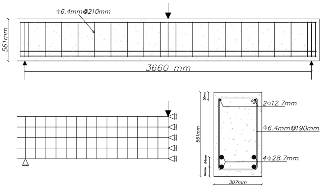
Figure 1: Technical drawing of the beam.

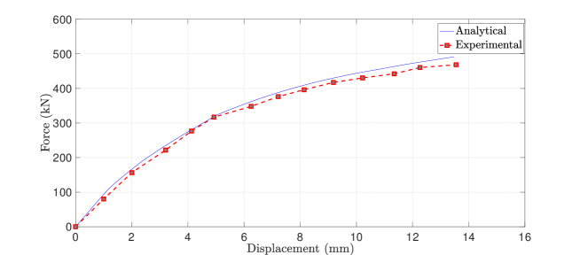
Figure 2: Load-displacement curve from the analytical model of the beam versus experimental data from [48].

In order to set up a stochastic model, we considered the initial concrete modulus of elasticity, which is one of the parameters that have significant effect on the response of a reinforced concrete member. There are many parametrizations proposed in literature. In this study, we used a formula from the FIB model code [38], which is

$$E_{ci}=E_{c0}\alpha_{E}\left(\frac{{f}_{cm}}{10}\right)^{\frac{1}{3}},$$ (31)

where $E_{ci}$ is the initial modulus of elasticity in MPa at the concrete age of $28$ days, $E_{c0}=21.5\,$GPa, $\alpha_{E}$ is a parameter that depend on the types of aggregate, for example equal $0.7$ for Sandstone aggregate and $0.9$ for Limestone aggregate, ${f}_{cm}$ is the actual compressive strength of concrete at an age of $28$ days in MPa. In formula (31), we considered$~{}\alpha_{E}$ as a random input parameter with uniform distribution and the mean value $0.8$. Two coefficients of variation (CoV) are considered for the random input parameter that equal $5.77\%$ and $10\%$. That is, the value of$~{}\alpha_{E}$ is uniformly distributed in the intervals $(0.72-0.88)$ and $(0.66-0.94)$, respectively. The initial concrete modulus of elasticity thus becomes stochastic, that is $E_{ci}\equiv E_{ci}(\xi)$.

Our goal in the setup is to find the stochastic expansion of the tangent stiffness matrix (18) via (28). This calculation uses an expansion of the the tangent modulus of elasticity and is repeated after every load increment. Based on the uniaxial stress-strain relationship in compression, see eq. (1), the tangent concrete modulus of elasticity is

$$E_{cT}=\frac{d\sigma_{c}}{d\epsilon_{c}}=E_{c1}\frac{(k-2\eta)-(k-2)\eta^{2}}{(1+(k-2)\eta)^{2}}.$$ (32)

Because $E_{cT}$ depends on $E_{ci}$, they are both stochastic, and in particular

$$E_{cT}(\xi)=E_{c1}\frac{\left(\frac{E_{ci}\left(\xi\right)}{E_{c1}}-2\frac{\epsilon_{c}}{\epsilon_{c1}}\right)-\left(\frac{E_{ci}(\xi)}{E_{c1}}-2\right)\left(\frac{\epsilon_{c}}{\epsilon_{c1}}\right)^{2}}{\left(1+\left(\frac{E_{ci}(\xi)}{E_{c1}}-2\right)\frac{\epsilon_{c}}{\epsilon_{c1}}\right)^{2}}.$$ (33)

Then, using also the values of$~{}\epsilon_{c}$ corresponding to the $n$th load increment, we project (33) on the gPC basis using numerical quadrature to calculate the expansion of the tangent concrete modulus of elasticity at the $n$th load increment

$$E_{cT}^{n}(\xi)=\sum_{i=1}^{n_{K}}E_{cTi}^{n}\psi_{i}(\xi).$$ (34)

Expansion (34) is then used to calculate expansion (18). In general, while by [12] when considering the expansion of the displacement (25) using gPC polynomials of degree$~{}p$ it would be possible to use gPC polynomials of degree up to$~{}2p$ in expansion (34), in the numerical experiments we used expansions of the same degree and we set $n_{K}=n_{\xi}$. In particular, we did not observe with $n_{K}>n_{\xi}$ any improvement of results in our numerical experiments.

In the numerical experiments, we show estimated probability density functions (PDFs) of the$~{}E_{cT}$, and then we particularly focus on the vertical displacement at the center of the beam$~{}u$, for which we also tabulate several other statistical estimates. We note that$~{}E_{cT}$ is pertinent to one element. We also compare the results of the stochastic Galerkin method (SG) to those obtained by the stochastic collocation (SC) and Monte Carlo (MC) methods. For the two spectral stochastic finite element methods, SC and SG, we used gPC polynomials of degree four and eight and Smolyak sparse grid. The results of the MC simulation are based on $10^{6}$ samples. As the validation criterion, we used the root mean square error (RMSE) of the vertical displacement at the center of the beam$~{}u$, defined as

$$\text{RMSE}=\sqrt{\frac{1}{n_{MC}}\sum_{i=1}^{n_{MC}}\left(u_{\star}\left(\xi^{(i)}\right)-u_{MC}\left(\xi^{(i)}\right)\right)^{2}},$$ (35)

where $\star$ indicates either SC or SG method. We also report in tables estimates of the mean $\mu$, standard deviation $\sigma$ and probability ${Pr}(u-ku_{m}\geq 0)$, where $u_{m}$ is the vertical displacement at the center of the beam corresponding to the deterministic problem (the parameters are set to the mean values), and values of $k$ are specified in the tables.

Figure 3 shows the estimated PDFs of the$~{}E_{cT}$ and the vertical displacement at the center of the beam for the case with $CoV=5.77\%$ at load increments $10$, $20$ and $87$, which is the final load increment in this case. A crack starts to propagate between the load increments $10$ and $20$ (specifically at the increment$~{}14$). Correspondingly, it can be observed that at the load increment 10 all PDF estimates are smooth and coincide, but at the increment$~{}20$ the PDF obtained by MC is oscillatory and the SC and SG methods provide a smooth interpolant. We also observe that the gPC polynomial with degree $p=8$ is relatively more oscillatory than the gPC polynomial with degree $p=4$. From the plots we anticipate that a polynomial of a very high degree, unfeasible for practical computations, would be needed in order to match the results of the MC simulation. Nevertheless, it turns out that even the low-degree gPC approximation provides an accurate quantitative insight into the response of the beam to loading. Such insight is provided by Table 1, which compares estimated values of the mean $\mu$ and standard deviation $\sigma$ for the displacement at center of the beam with $CoV=5.77\%$ using Monte Carlo (MC), stochastic Galerkin (SG) and stochastic collocation (SC) methods with gPC degrees $p=4$ and $8$, and an assessment of the methods using both the RMSE value (35). Table 2 then provides estimates of probability $\operatorname{Pr}(u-\widetilde{u}\geq 0)$, where $u$ is the displacement at the center of the beam from the stochastic problem and different setting of $\widetilde{u}$, in which $u_{m}$ is the displacement at the center of the beam from the deterministic problem with the mean value parameters. We see a good agreement of all methods in all indicators $\mu$, $\sigma$ and $\Pr$. In fact, from the results we cannot discern any improvement by increasing the gPC degree.

Figure 4, Table 3 and Table 4 then show results corresponding to $CoV=10\%$. Comparing to the case with $CoV=5.77\%$, we see that all PDFs have larger support, but the qualitative behavior of the solutions is similar to the previous case. In particular, at the load increment$~{}10$, the results of all methods match, and after the crack starts to propagate at higher load increments, the gPC methods provide a smooth interpolation to the MC solution. Nevertheless, in all cases the statistical indicators $\mu$, $\sigma$ and $\Pr$ reported in Table 3 and Table 4 are again in a good agreement with Monte Carlo simulation.

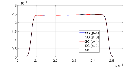
(a) $E_{cT}$ at load increment 10

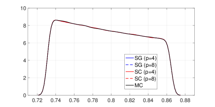
(b) displacement at load increment 10

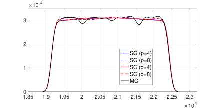
(c) $E_{cT}$ at load increment 20

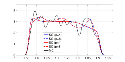
(d) displacement at load increment 20

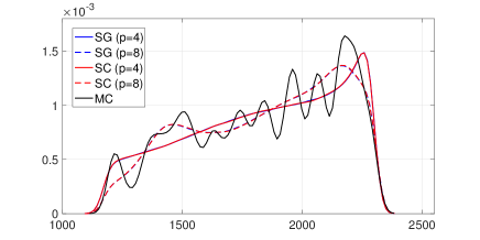
(e) $E_{cT}$ at load increment 87

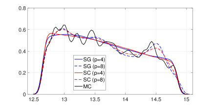
(f) displacement at load increment 87

Figure 3: Estimated PDFs of $E_{cT}$ and the displacement at center of the beam during the loading, $CoV=5.77\%$.

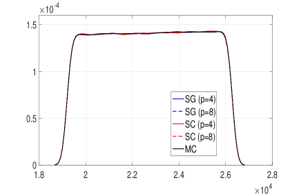
(a) $E_{cT}$ at load increment 10

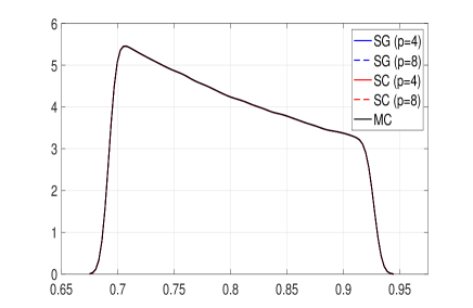
(b) displacement at load increment 10

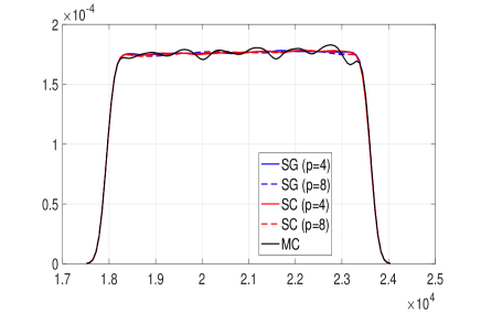
(c) $E_{cT}$ at load increment 20

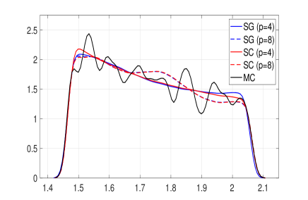
(d) displacement at load increment 20

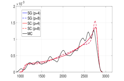
(e) $E_{cT}$ at load increment 86

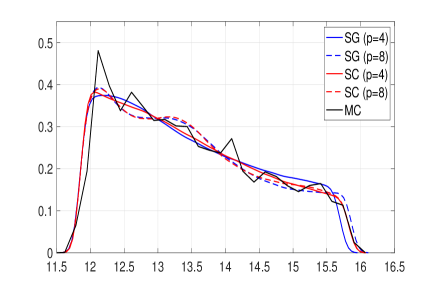
(f) displacement at load increment 86

Figure 4: Estimated PDFs of $E_{cT}$ and the displacement at center of the beam during the loading, $CoV=10\%$.

Table 1: Displacement at center of the beam with $CoV=5.77\%$: estimated values of the mean $\mu$ and standard deviation $\sigma$ by Monte Carlo (MC), stochastic Galerkin (SG) and stochastic collocation (SC) methods with gPC degrees $p=4$ and $8$, comparison of the methods using root mean square error (RMSE), see eq. (35).

method	$\mu$	$\sigma$	$\operatorname{RMSE}$
load increment 10
MC	$7.9414\times 10^{-1}$	$3.8566\times 10^{-2}$	-
SG, $p=4$	$7.9415\times 10^{-1}$	$3.8567\times 10^{-2}$	$4.7201\times 10^{-2}$
SG, $p=8$	$7.9415\times 10^{-1}$	$3.8567\times 10^{-2}$	$4.7201\times 10^{-2}$
SC, $p=4$	$7.9414\times 10^{-1}$	$3.8566\times 10^{-2}$	$4.7201\times 10^{-2}$
SC, $p=8$	$7.9415\times 10^{-1}$	$3.8567\times 10^{-2}$	$4.7201\times 10^{-2}$
load increment 20
MC	$1.7267$	$9.8225\times 10^{-2}$	-
SG, $p=4$	$1.7261$	$9.8658\times 10^{-2}$	$1.2050\times 10^{-1}$
SG, $p=8$	$1.7260$	$9.7058\times 10^{-2}$	$1.1952\times 10^{-1}$
SC, $p=4$	$1.7263$	$9.8590\times 10^{-2}$	$1.2046\times 10^{-1}$
SC, $p=8$	$1.7260$	$9.7035\times 10^{-2}$	$1.1951\times 10^{-1}$
load increment 87
MC	$13.6311$	$6.1582\times 10^{-1}$	-
SG, $p=4$	$13.6280$	$6.1808\times 10^{-1}$	$7.5516\times 10^{-1}$
SG, $p=8$	$13.6401$	$6.2000\times 10^{-1}$	$7.5639\times 10^{-1}$
SC, $p=4$	$13.6275$	$6.1693\times 10^{-1}$	$7.5445\times 10^{-1}$
SC, $p=8$	$13.6309$	$6.1700\times 10^{-1}$	$7.5449\times 10^{-1}$

Table 2: Estimated probability $\operatorname{Pr}(u-\widetilde{u}\geq 0)$ in %, where $u$ is the displacement at the center of the beam from the stochastic problem with $CoV=5.77\%$ and different setting of $\widetilde{u}$, in which $u_{m}$ is the displacement at the center of the beam from the deterministic problem with the mean value parameters.

method	$\widetilde{u}=u_{m}$	$\widetilde{u}=1.02u_{m}$	$\widetilde{u}=1.04u_{m}$	$\widetilde{u}=1.06u_{m}$	$\widetilde{u}=1.08$	$\widetilde{u}=1.10u_{m}$
load increment 10
MC	$48.56\,\%$	$36.93\,\%$	$25.75\,\%$	$14.97\,\%$	$4.56\,\%$	$0\,\%$
SG, $p=4$	$48.57\,\%$	$36.95\,\%$	$25.74\,\%$	$14.95\,\%$	$4.55\,\%$	$0\,\%$
SG, $p=8$	$48.57\,\%$	$36.95\,\%$	$25.74\,\%$	$14.95\,\%$	$4.55\,\%$	$0\,\%$
SC, $p=4$	$48.57\,\%$	$36.95\,\%$	$25.74\,\%$	$14.95\,\%$	$4.55\,\%$	$0\,\%$
SC, $p=8$	$48.57\,\%$	$36.95\,\%$	$25.74\,\%$	$14.95\,\%$	$4.55\,\%$	$0\,\%$
load increment 20
MC	$49.22\,\%$	$38.79\,\%$	$28.11\,\%$	$20.98\,\%$	$9.57\,\%$	$1.87\,\%$
SG, $p=4$	$49.17\,\%$	$38.73\,\%$	$28.49\,\%$	$18.83\,\%$	$10.14\,\%$	$2.44\,\%$
SG, $p=8$	$48.24\,\%$	$37.34\,\%$	$28.34\,\%$	$19.94\,\%$	$9.70\,\%$	$1.44\,\%$
SC, $p=4$	$49.27\,\%$	$38.84\,\%$	$28.64\,\%$	$18.97\,\%$	$10.15\,\%$	$2.25\,\%$
SC, $p=8$	$48.30\,\%$	$37.43\,\%$	$28.35\,\%$	$19.88\,\%$	$9.67\,\%$	$1.51\,\%$
load increment 87
MC	$47.09\,\%$	$34.33\,\%$	$24.16\,\%$	$12.54\,\%$	$3.81\,\%$	$0\,\%$
SG, $p=4$	$46.98\,\%$	$34.50\,\%$	$23.24\,\%$	$13.12\,\%$	$3.84\,\%$	$0\,\%$
SG, $p=8$	$46.87\,\%$	$34.68\,\%$	$24.90\,\%$	$14.35\,\%$	$3.34\,\%$	$0\,\%$
SC, $p=4$	$47.21\,\%$	$34.50\,\%$	$23.04\,\%$	$12.89\,\%$	$3.84\,\%$	$0\,\%$
SC, $p=8$	$46.83\,\%$	$34.71\,\%$	$24.39\,\%$	$13.77\,\%$	$3.25\,\%$	$0\,\%$

Table 3: Displacement at center of the beam with $CoV=10\%$: the headers are the same as in Table 1.

	$\mu$	$\sigma$	$\operatorname{RMSE}$
load increment 10
MC	$7.9804\times 10^{-1}$	$6.7548\times 10^{-2}$	-
SG, $p=4$	$7.9804\times 10^{-1}$	$6.7548\times 10^{-2}$	$2.5263\times 10^{-6}$
SG, $p=8$	$7.9804\times 10^{-1}$	$6.7548\times 10^{-2}$	$0.0332\times 10^{-6}$
SC, $p=4$	$7.9804\times 10^{-1}$	$6.7548\times 10^{-2}$	$2.5284\times 10^{-6}$
SC, $p=8$	$7.9804\times 10^{-1}$	$6.7548\times 10^{-2}$	$0.0331\times 10^{-6}$
load increment 20
MC	$1.7365$	$1.7224\times 10^{-1}$	-
SG, $p=4$	$1.7367$	$1.7247\times 10^{-1}$	$3.3543\times 10^{-3}$
SG, $p=8$	$1.7363$	$1.7242\times 10^{-1}$	$3.4802\times 10^{-3}$
SC, $p=4$	$1.7365$	$1.7255\times 10^{-1}$	$3.0136\times 10^{-3}$
SC, $p=8$	$1.7365$	$1.7247\times 10^{-1}$	$3.3217\times 10^{-3}$
load increment 86
MC	$13.4660$	$1.0815\times 10^{0}$	-
SG, $p=4$	$13.4496$	$1.0789\times 10^{0}$	$5.6684\times 10^{-2}$
SG, $p=8$	$13.4615$	$1.1007\times 10^{0}$	$5.2660\times 10^{-2}$
SC, $p=4$	$13.4568$	$1.0911\times 10^{0}$	$4.9047\times 10^{-2}$
SC, $p=8$	$13.4565$	$1.0907\times 10^{0}$	$5.0035\times 10^{-2}$

Table 4: Estimated probability $\operatorname{Pr}(u-\widetilde{u}\geq 0)$ in %, where $u$ is the displacement at the center of the beam from the stochastic problem with $CoV=10\%$ and different setting of $\widetilde{u}$, in which $u_{m}$ is the displacement at the center of the beam from the deterministic problem with the mean value parameters.

method	$\widetilde{u}=u_{m}$	$\widetilde{u}=1.04u_{m}$	$\widetilde{u}=1.08u_{m}$	$\widetilde{u}=1.12u_{m}$	$\widetilde{u}=1.16u_{m}$	$\widetilde{u}=1.20u_{m}$
load increment 10
MC	$47.51\,\%$	$34.40\,\%$	$22.26\,\%$	$11.00\,\%$	$0.52\,\%$	$0\,\%$
SG, $p=4$	$47.51\,\%$	$34.40\,\%$	$22.26\,\%$	$11.00\,\%$	$0.52\,\%$	$0\,\%$
SG, $p=8$	$47.51\,\%$	$34.40\,\%$	$22.26\,\%$	$11.00\,\%$	$0.52\,\%$	$0\,\%$
SC, $p=4$	$47.51\,\%$	$34.40\,\%$	$22.26\,\%$	$11.00\,\%$	$0.52\,\%$	$0\,\%$
SC, $p=8$	$47.51\,\%$	$34.40\,\%$	$22.26\,\%$	$11.00\,\%$	$0.52\,\%$	$0\,\%$
load increment 20
MC	$47.47\,\%$	$36.35\,\%$	$24.72\,\%$	$15.96\,\%$	$6.52\,\%$	$0\,\%$
SG, $p=4$	$47.68\,\%$	$36.67\,\%$	$26.21\,\%$	$16.12\,\%$	$6.15\,\%$	$0\,\%$
SG, $p=8$	$47.96\,\%$	$35.72\,\%$	$25.45\,\%$	$16.17\,\%$	$6.29\,\%$	$0\,\%$
SC, $p=4$	$47.64\,\%$	$36.53\,\%$	$25.98\,\%$	$15.97\,\%$	$6.37\,\%$	$0\,\%$
SC, $p=8$	$47.99\,\%$	$35.91\,\%$	$25.47\,\%$	$16.08\,\%$	$6.46\,\%$	$0\,\%$
load increment 86
MC	$44.69\,\%$	$31.16\,\%$	$20.26\,\%$	$10.91\,\%$	$2.70\,\%$	$0\,\%$
SG, $p=4$	$44.91\,\%$	$31.53\,\%$	$20.09\,\%$	$10.13\,\%$	$1.20\,\%$	$0\,\%$
SG, $p=8$	$44.79\,\%$	$30.48\,\%$	$19.82\,\%$	$11.26\,\%$	$3.47\,\%$	$0\,\%$
SC, $p=4$	$44.94\,\%$	$31.23\,\%$	$19.92\,\%$	$10.58\,\%$	$2.66\,\%$	$0\,\%$
SC, $p=8$	$44.70\,\%$	$30.49\,\%$	$19.89\,\%$	$10.86\,\%$	$2.73\,\%$	$0\,\%$

3.4 Example 2: Reinforced concrete shear wall

We also consider a reinforced concrete shear wall as specimen SH-L tested in [49]. A detailed drawing is shown in Figure 5. The spatial discretization uses a two-dimensional mesh with $72$ finite elements and $182$ degree of freedom under plane stress conditions. Material properties of the shear wall are set as follows: the maximum compressive stress of the concrete $\acute{f}_{c}=44.7\,$MPa, yield stress of the horizontal and vertical reinforcement $f_{sy1}=460\,$MPa. The wall is first subjected to a vertical load of $357$KN, then the lateral load is applied incrementally. First, we implemented the deterministic nonlinear finite element procedure as discussed in Section 3.1 in Matlab. A comparison of the load-horizontal displacement curves from the deterministic model with the experiment [49] can be seen in Figure 6. A good agreement between numerical and experimental results can be seen throughout the entire load-displacement range.

Figure 5: Technical drawing of the shear wall.

Figure 6: Load-displacement curve from the analytical model of the shear wall versus experimental data from [49].

For the stochastic model, we considered the maximum compressive stress of the concrete $\acute{f}_{c}$, as a random input parameter with uniform distribution. To consider the spatial variability of the random parameter, we assume that mean of the maximum compressive stress of the concrete changes linearly from $(44.7+1.5)$MPa in the lowest mesh row to $(44.7-1.5)$MPa in the uppermost mesh row. The coefficients of variation (CoV) is considered equal to $5\%$.

In the numerical experiments we show estimated probability density function (PDF) of the displacement $u$ at the location of the applied lateral load, and we also tabulate several other statistical estimates including RMSE from (35). We compare the results of the stochastic Galerkin method (SG) to those obtained by stochastic collocation (SC) and Monte Carlo (MC) methods. For the two spectral stochastic finite element methods, SC and SG, we used gPC polynomials of degree 4 and 8 and Smolyak sparse grid. The results of the MC simulation are based on $10^{6}$ samples.

Figure 7 shows the estimated PDFs of the displacement at the location of the lateral load at top of the shear wall at load increments $5$, $10$, $20$ and $50$, which is the final load increment. A crack starts to propagate between the load increments $10$ and $20$ since that is when the PDF obtained by MC becomes oscillatory. It can be also seen, similarly as for the beam, that both SC and SG methods provide a smooth interpolant with degree $p=8$ relatively more oscillatory than with degree $p=4$. Table 5 then compares estimated values of the mean $\mu$ and standard deviation $\sigma$ for the displacement at the location of the lateral load at top of the shear wall using MC, SG and SC methods and an assessment of the methods using both the RMSE and probability estimates. It can be seen again that all methods are in quite a good agreement with Monte Carlo simulation, and this holds in particular for the probability estimates.

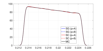
(a) displacement at load increment 5

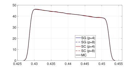
(b) displacement at load increment 10

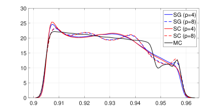
(c) displacement at load increment 20

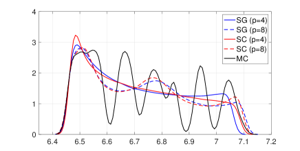
(d) displacement at load increment 50

Figure 7: Estimated PDFs of the displacement at the location of the lateral load at top of the shear wall during the loading.

Table 5: Displacement at the location of the lateral load at top of the shear wall: values of the mean $\mu$ and standard deviation $\sigma$ by Monte Carlo (MC), stochastic Galerkin (SG) and stochastic collocation (SC) methods with gPC degrees $p=4$ and $8$, comparison of the methods using root mean square error (RMSE), and estimated probability $\operatorname{Pr}(u-\widetilde{u}\geq 0)$ in %, where $u$ is the displacement from the stochastic problem and different setting of $\widetilde{u}$, in which $u_{m}$ is the displacement from the deterministic problem with the mean value parameters.

method	$\mu$	$\sigma$	$\operatorname{RMSE}$	$\widetilde{u}=u_{m}$	$\widetilde{u}=1.01u_{m}$	$\widetilde{u}=1.02u_{m}$
load increment 5
MC	$2.1876\times 10^{-1}$	$3.3858\times 10^{-3}$	-	$48.56\,\%$	$30.76\,\%$	$13.27\,\%$
SG, $p=4$	$2.1875\times 10^{-1}$	$3.3860\times 10^{-3}$	$4.7847\times 10^{-3}$	$48.98\,\%$	$30.70\,\%$	$13.23\,\%$
SG, $p=8$	$2.1875\times 10^{-1}$	$3.3860\times 10^{-3}$	$4.7847\times 10^{-3}$	$48.98\,\%$	$30.70\,\%$	$13.23\,\%$
SC, $p=4$	$2.1875\times 10^{-1}$	$3.3860\times 10^{-3}$	$4.7847\times 10^{-3}$	$48.98\,\%$	$30.70\,\%$	$13.23\,\%$
SC, $p=8$	$2.1875\times 10^{-1}$	$3.3860\times 10^{-3}$	$4.7847\times 10^{-3}$	$48.98\,\%$	$30.70\,\%$	$13.23\,\%$
load increment 10
MC	$4.3994\times 10^{-1}$	$6.8147\times 10^{-3}$	-	$49.09\,\%$	$30.77\,\%$	$13.30\,\%$
SG, $p=4$	$4.3993\times 10^{-1}$	$6.8147\times 10^{-3}$	$9.6302\times 10^{-3}$	$48.99\,\%$	$30.71\,\%$	$13.25\,\%$
SG, $p=8$	$4.3993\times 10^{-1}$	$6.8153\times 10^{-3}$	$9.6305\times 10^{-3}$	$48.99\,\%$	$30.71\,\%$	$13.26\,\%$
SC, $p=4$	$4.3993\times 10^{-1}$	$6.8148\times 10^{-3}$	$9.6302\times 10^{-3}$	$48.99\,\%$	$30.71\,\%$	$13.25\,\%$
SC, $p=8$	$4.3993\times 10^{-1}$	$6.8153\times 10^{-3}$	$9.6305\times 10^{-3}$	$48.99\,\%$	$30.71\,\%$	$13.26\,\%$
load increment 20
MC	$9.2863\times 10^{-1}$	$1.4732\times 10^{-2}$	-	$48.43\,\%$	$29.91\,\%$	$12.25\,\%$
SG, $p=4$	$9.2851\times 10^{-1}$	$1.4604\times 10^{-2}$	$2.0728\times 10^{-2}$	$48.56\,\%$	$29.07\,\%$	$13.15\,\%$
SG, $p=8$	$9.2861\times 10^{-1}$	$1.4755\times 10^{-2}$	$2.0835\times 10^{-2}$	$48.31\,\%$	$29.77\,\%$	$13.25\,\%$
SC, $p=4$	$9.2853\times 10^{-1}$	$1.4648\times 10^{-2}$	$2.0759\times 10^{-2}$	$48.65\,\%$	$28.95\,\%$	$13.18\,\%$
SC, $p=8$	$9.2862\times 10^{-1}$	$1.4763\times 10^{-2}$	$2.0840\times 10^{-2}$	$48.28\,\%$	$29.78\,\%$	$13.31\,\%$
load increment 50
MC	$6.6636\times 10^{0}$	$3.0779\times 10^{-1}$	-	$55.07\,\%$	$45.23\,\%$	$31.54\,\%$
SG, $p=4$	$6.7119\times 10^{0}$	$0.8756\times 10^{-1}$	$3.2090\times 10^{-1}$	$53.02\,\%$	$43.04\,\%$	$33.91\,\%$
SG, $p=8$	$6.7216\times 10^{0}$	$0.9085\times 10^{-1}$	$3.2220\times 10^{-1}$	$56.25\,\%$	$46.38\,\%$	$34.91\,\%$
SC, $p=4$	$6.7130\times 10^{0}$	$0.8872\times 10^{-1}$	$3.2127\times 10^{-1}$	$53.42\,\%$	$43.17\,\%$	$33.69\,\%$
SC, $p=8$	$6.7212\times 10^{0}$	$0.9071\times 10^{-1}$	$3.2215\times 10^{-1}$	$56.47\,\%$	$46.41\,\%$	$34.24\,\%$

4 Iterative solution of the linearized systems

The solution of the linearized stochastic Galerkin systems of equations (22) may be a computationally expensive task due to its size, and also with respect to the large number of load increments and steps, use of direct methods may be prohibitive. Therefore, we also studied the problem of solving the stochastic Galerkin systems of equations by iterative methods. Since the associated matrices are symmetric and positive definite, we used conjugate gradient (CG) method [50]. However, the matrices are typically also ill-conditioned, and construction of efficient preconditioners becomes an important task for a practical implementation. In this study, we use two preconditioners, the first one is the mean-based preconditioner [16, 17] and the second one is the hierarchical Gauss-Seidel preconditioner [21].

4.1 Mean-based preconditioner

The stiffness matrix derived from the SGFEM formulation has a particular structure that can be exploited during the process of solving the algebraic system of equations. In general, the matrix$~{}K_{1}^{n}$ in equation (18) corresponds to the mean properties of the system, and it has a much more considerable contribution than the other $K_{i}^{n}$’s that represent random fluctuations of the system from the mean, especially for smaller values of$~{}CoV$. Since the submatrix $K_{1}^{n}$ contributes only to the block-diagonal of the stochastic Galerkin matrix, the resulting system of linear equations exhibits a strong block-diagonal dominance if the random properties represent only small fluctuations from the mean values. Then, the mean-based preconditioner, given in a matrix form as $I_{n_{\xi}}\otimes K_{1}^{n}$, will be a good approximation to the stochastic Galerkin matrix$~{}\mathbf{K}^{n}$. This block-diagonal matrix has the great advantage because it can be inverted by inverting each block along the block-diagonal independently. On the other hand, in systems with large random fluctuations, the off-diagonal blocks have a much stronger contribution. For these cases the mean-based preconditioner may not improve the convergence rate, because it does not approximate the system matrix sufficiently.

4.2 Hierarchical Gauss-Seidel preconditioner

The block structure of the global stochastic stiffness Galerkin matrix (23) depends on the tensor given by the values$~{}c_{jkm}$. We will now consider that the stochastic Galerkin matrix$~{}\mathbf{K}^{n}$ in (23) has a hierarchical structure, cf. Fig. 8, given as

$$\mathbf{K}^{n}=\begin{bmatrix}A_{1}&&B_{1}&&\\ &\ddots&&&\\ C_{l}&&A_{l}&&B_{l}\\ &&&\ddots&\\ &&C_{p+1}&&A_{p+1}\end{bmatrix},$$ (36)

where $A_{1}=K_{1}^{n}$ is the matrix of the mean. The decomposition (36) is used to formulate the hierarchical Gauss-Seidel preconditioner [21]. A matrix-vector multiplication by the stochastic Galerkin matrix is in an iterative solver performed using $K_{(k,m)}^{n}=\sum_{j=1}^{n_{\xi}}c_{jkm}{K}_{j}^{n}$, so we use only the constants $c_{jkm}$ and matrices ${K}_{j}^{n}$. The same strategy is used in the preconditioner for multiplications by the submatrices $B_{l}$ and $C_{l}$, see (36), and the solves with the diagonal submatrices are approximated by the block-diagonal solves with the mean matrix, that is $A_{l}\approx\widetilde{A}_{l}=I\otimes A_{1}$ of the appropriate size. Finally, let us introduce the following notation for a vector $x_{l}$, where $l=1,\dots,p+1$, cf. Fig. 8, as

$$x_{l}=x_{(1:l)}=\begin{bmatrix}x_{(1)}\\ x_{(2)}\\ \vdots\\ x_{(l)}\end{bmatrix}$$ (37)

The hierarchical Gauss-Seidel preconditioner (ahGS): $r_{p+1}\longmapsto\upsilon_{p+1}$ for the system (22) is defined as follows [21]:

Set the initial solution $v_{p+1}=0$ and update it in the following steps,

$$\upsilon_{(1)}=A_{1}^{-1}(r_{(1)}-B_{1}\upsilon_{(2:p+1)})$$ (38)

for $l=2,\cdots,p$,

$$\upsilon_{(l)}=\widetilde{A}_{l}^{-1}(r_{(l)}-C_{l}\upsilon_{(1:l-1)}-B_{l}\upsilon_{(l+1:p+1)})$$ (39)

end

$$\upsilon_{(p+1)}=\widetilde{A}_{p+1}^{-1}(r_{(p+1)}-C_{p}\upsilon_{(1:p)})$$ (40)

for $l=p,\cdots,2$,

$$\upsilon_{(l)}=\widetilde{A}_{l}^{-1}(r_{(l)}-C_{l}\upsilon_{(1:l-1)}-B_{l}\upsilon_{(l+1:p+1)})$$ (41)

end

$$\upsilon_{(1)}=A_{1}^{-1}(r_{(1)}-B_{1}\upsilon_{(2:p+1)})$$ (42)

Since we initialize $v_{p}=0$, the multiplications by $B_{l}$, $l=1,\dots,p$, vanish from (38) and (39).

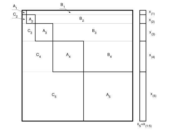
Figure 8: The hierarchical structure of the stochastic Galerkin matrix.

4.3 Numerical experiments

We tested the solvers using both the beam and the shear wall. For solving the system of equations (22), we used the CG method with the mean-based (MB) and hierarchical Gauss-Seidel (ahGS) preconditioners from Sections 4.1 and 4.2, respectively. As the stopping criterion we used a reduction of the 2-norm of the residual by a factor$~{}10^{-8}$.

For the beam, Figure 9 shows the numbers of iterations in each load increment. We see that for all load increments the ahGS preconditioner reduces the iteration count to approximately one half compared to the MB preconditioner. For both preconditioners, the iteration count increases slightly for the higher degree of the gPC polynomial, but the increase is less pronounced for the ahGS preconditioner. The same observation can be made for an increase of$~{}CoV$ by comparing the left and right panels in Figure 9. We can also easily deduce from Figure 9 that the crack starts to develop in load increment $14$. In particular, the number of iterations is quite small and constant during the initial load increments, but the character of the problem changes and becomes challenging for the iterative solvers once the crack starts to develop. The numbers of iterations slowly increase as the loading progresses, but the overall growth of the iteration count is somewhat slower for the ahGS preconditioner. Figure 10 then shows residual history at load increment$~{}10$ and at the last load increments for the two choices of $CoV$. This further illustrates the discussion above, and in particular the efficiency gained due to the use of the ahGS preconditioner throughout the entire loading process.

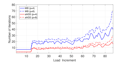
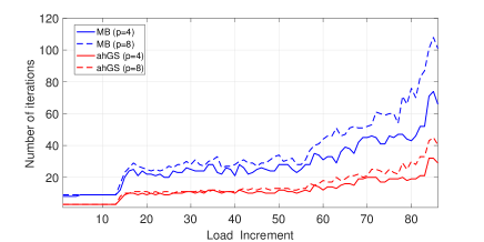
Figure 9: Iteration count for the beam at load increments with different preconditioners for $CoV=5.77\%$ (left) and $10\%$ (right).

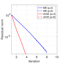
(a) $CoV\ 5.77\%$, increment 10

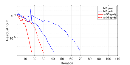
(b) $CoV\ 5.77\%$, increment 87

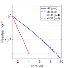
(c) $CoV\ 10\%$, increment 10

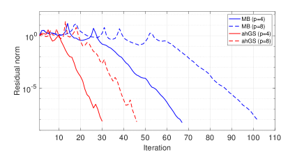
(d) $CoV\ 10\%$, increment 86

Figure 10: Residual norm at each iteration for the beam with $CoV=5.77\%$ (top) and $10\%$ (bottom).

For the shear wall, the Figure 11 shows the numbers of iterations in each load increment. We see, similarly as for the beam, that for all load increments the ahGS preconditioner reduces the iteration count compared to the MB preconditioner to approximately one half. And in a similar observation for both preconditioners, the iteration count increases slightly for the higher degree of the gPC polynomial, but the increase is less pronounced for the ahGS preconditioner. Figure 12 then shows residual history at load increment$~{}5$, $~{}10$, $~{}20$ and $50$, which is the last load increment. The plots further illustrate the discussion above, and in particular the efficiency gained due to the use of the ahGS preconditioner throughout the entire loading process.

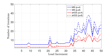
Figure 11: Iteration count at load increments with different preconditioners for the shear wall.

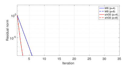
(a) increment 5

(b) increment 10

(c) increment 20

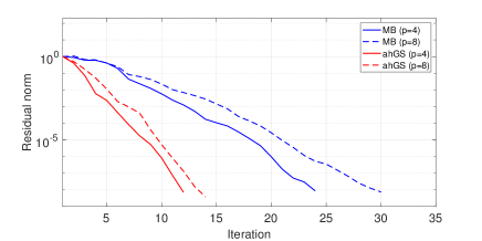
(d) increment 50

Figure 12: Residual norm at each iteration for the shear wall.

5 Conclusion

A new methodology for the extension of the stochastic Galerkin finite element method (SGFEM) is presented to efficiently propagate the uncertainty in nonlinear elasticity problems. It can be applied, in general, to models of reinforced concrete members with random material properties. In the nonlinear SGFEM, the linearization scheme based on the modified Newton-Raphson method. By directly updating the gPC expansions of the strain and stress vectors between each loading step and updating the stiffness matrix at the first step of load increments, the stochastic displacements at each level of loading are obtained. The performance of the nonlinear SGFEM is tested using a reinforced concrete beam with random initial concrete modulus of elasticity and a shear wall with random maximum compressive stress of concrete. We illustrate by numerical experiments that even a low-degree gPC polynomial provides a smooth interpolant to the full solution provided by Monte Carlo simulation, and it provides an accurate estimate of several statistical indicators associated with the probability distribution of the response of the structure. Since the linear systems associated with the use of the stochastic Galerkin method may be very large and many of them need to be solved due to the incremental loading, we also studied their iterative solution using preconditioned conjugate gradient method with mean-based (MB) and hierarchical Gauss-Seidel (ahGS) preconditioners. Numerical experiments show that the ahGS preconditioner reduces the number of iterations to approximately one half of iterations needed using the MB preconditioner. Using the proposed methodology, it becomes practical to accurately approximate the distribution of the structural response, which could be used for risk assessment and more efficient engineering design of nonlinear structures that include uncertainty in the material properties.

- [1] Fishman, G., Monte Carlo: Concepts, Algorithms, and Applications, Springer-Verlag New York, 1996.
- [2] Caflisch, R. E., Monte Carlo and quasi-Monte Carlo methods, Acta Numerica, 7:1–49, 1998.
- [3] Kleiber, M. and Hien, T. D., The stochastic finite element method: basic perturbation technique and computer implementation, Wiley, 1992.
- [4] Kaminski, M. M., The Stochastic Perturbation Method for Computational Mechanics, John Wiley & Sons, 2013.
- [5] Ghanem, R. G. and Spanos, P. D., Stochastic Finite Elements: A Spectral Approach, Springer-Verlag New York, Inc., New York, NY, USA, 1991. (Revised edition by Dover Publications, 2003).
- [6] Stefanou, G., The stochastic finite element method: past, present and future, Computer Methods in Applied Mechanics and Engineering, 198(9–12):1031–1051, 2009.
- [7] Xiu, D. and Karniadakis, G. E., The Wiener-Askey polynomial chaos for stochastic differential equations, SIAM Journal on Scientific Computing, 24(2):619–644, 2002.
- [8] Babuška, I., Nobile, F., and Tempone, R., A stochastic collocation method for elliptic partial differential equations with random input data, SIAM Review, 52(2):317–355, 2010, (The paper originally appeared in SIAM Journal on Numerical Analysis, Volume 45, Number 3, 2007, pages 1005–1034.).
- [9] Berveiller, M., Sudret, B., and Lemaire, M., Stochastic finite element: a non intrusive approach by regression, European Journal of Computational Mechanics/Revue Européenne de Mécanique Numérique, 15(1–3):81–92, 2006.
- [10] Gunzburger, M. D., Webster, C. G., and Zhang, G., Stochastic finite element methods for partial differential equations with random input data, Acta Numer., 23:521–650, 2014.
- [11] Babuška, I., Tempone, R., and Zouraris, G. E., Galerkin finite element approximations of stochastic elliptic partial differential equations, SIAM Journal on Numerical Analysis, 42(2):800–825, 2004.
- [12] Matthies, H. G. and Keese, A., Galerkin methods for linear and nonlinear elliptic stochastic partial differential equations, Comput. Meth. Appl. Mech. Eng., 194(12–16):1295–1331, 2005.
- [13] Sudret, B., Polynomial chaos expansions and stochastic finite element methods, Risk and Reliability in Geotechnical Engineering, pp. 265–300, 2015.
- [14] Giraldi, L., Litvinenko, A., Liu, D., Matthies, H. G., and Nouy, A., To be or not to be intrusive? The solution of parametric and stochastic equations—the “plain vanilla” Galerkin case, SIAM Journal on Scientific Computing, 36(6):A2720–A2744, 2014.
- [15] Ghosh, D., Probabilistic interpretation of conjugate gradient iterations in spectral stochastic finite element method, AIAA Journal, 52(6):1313–1316, 2014.
- [16] Pellissetti, M. F. and Ghanem, R. G., Iterative solution of systems of linear equations arising in the context of stochastic finite elements, Advances in Engineering Software, 31(8–9):607–616, 2000.
- [17] Powell, C. E. and Elman, H. C., Block-diagonal preconditioning for spectral stochastic finite-element systems, IMA Journal of Numerical Analysis, 29(2):350–375, 2009.
- [18] Ullmann, E., A Kronecker product preconditioner for stochastic Galerkin finite element discretizations, SIAM Journal on Scientific Computing, 32(2):923–946, 2010.
- [19] Ullmann, E., Elman, H. C., and Ernst, O. G., Efficient iterative solvers for stochastic Galerkin discretizations of log-transformed random diffusion problems, SIAM Journal on Scientific Computing, 34(2):A659–A682, 2012.
- [20] Sousedík, B., Ghanem, R. G., and Phipps, E. T., Hierarchical Schur complement preconditioner for the stochastic Galerkin finite element methods, Numerical Linear Algebra with Applications, 21(1):136–151, 2014.
- [21] Sousedík, B. and Ghanem, R. G., Truncated hierarchical preconditioning for the stochastic Galerkin FEM, International Journal for Uncertainty Quantification, 4(4):333–348, 2014.
- [22] Sarkar, A., Benabbou, N., and Ghanem, R., Domain decomposition of stochastic PDEs: theoretical formulations, International Journal for Numerical Methods in Engineering, 77(5):689–701, 2009.
- [23] Ghosh, D., Avery, P., and Farhat, C., A FETI-preconditioned conjugate gradient method for large-scale stochastic finite element problems, International Journal for Numerical Methods in Engineering, 80(6–7):914–931, 2009.
- [24] Subber, W. and Sarkar, A., A domain decomposition method of stochastic PDEs: An iterative solution techniques using a two-level scalable preconditioner, Journal of Computational Physics, 257, Part A:298–317, 2014.
- [25] Subber, W. and Loisel, S., Schwarz preconditioners for stochastic elliptic PDEs, Computer Methods in Applied Mechanics and Engineering, 272:34–57, 2014.
- [26] Rosseel, E. and Vandewalle, S., Iterative solvers for the stochastic finite element method, SIAM Journal on Scientific Computing, 32(1):372–397, 2010.
- [27] Brezina, M., Doostan, A., Manteuffel, T., McCormick, S., and Ruge, J., Smoothed aggregation algebraic multigrid for stochastic PDE problems with layered materials, Numerical Linear Algebra with Applications, 21(2):239–255, 2014.
- [28] Osborn, S. V., Multilevel solution strategies for the stochastic Galerkin method, PhD thesis, Texas Tech University, Department of Mathematics and Statistics, 2015.
- [29] Keese, A. and Matthies, H. G., Hierarchical parallelisation for the solution of stochastic finite element equations, Computers & Structures, 83(14):1033–1047, 2005.
- [30] Ernst, O. G. and Ullmann, E., Stochastic Galerkin matrices, SIAM Journal on Matrix Analysis and Applications, 31(4):1848–1872, 2010.
- [31] Coulier, P., Pouransari, H., and Darve, E., The inverse fast multipole method: using a fast approximate direct solver as a preconditioner for dense linear systems, SIAM Journal on Scientific Computing, 39(3):A761–A796, 2017.
- [32] Kubínová, M. and Pultarová, I., Block preconditioning of stochastic Galerkin problems: new two-sided guaranteed spectral bounds, SIAM/ASA Journal on Uncertainty Quantification, 8(1):88–113, 2020.
- [33] Bespalov, A., Loghin, D., and Youngnoi, R., Truncation preconditioners for stochastic Galerkin finite element discretizations, SIAM Journal on Scientific Computing, 43(5):S92–S116, 2021.
- [34] Lacour, M., Macedo, J., and Abrahamson, N. A., Stochastic finite element method for non-linear material models, Computers and Geotechnics, 125:103641, 2020.
- [35] Bažant, Z. P. and Nilson, A. H., State-of-the-art report on finite element analysis of reinforced concrete, American Society of Civil Engineers, New York, USA, 1982. (Task Committee on Finite Element Analysis of Reinforced Concrete Structures).
- [36] Kupfer, H., Hilsdorf, H. K., and Rusch, H., Behavior of concrete under biaxial stresses, ACI Journal Proceedings, 66(8):656–666, 1969.
- [37] Darwin, D. and Pecknold, D. A., Nonlinear biaxial stress-strain law for concrete, Journal of the Engineering Mechanics Division, 103(2):229–241, 1977.
- [38] Taerwe, L. and Matthys, S., FIB model code for concrete structures 2010, Ernst & Sohn, Wiley, 2013. (Federation Internationale du Beton/International Federation for Structural Concrete (FIB), FIB special activity group).
- [39] Chen, W.-F., Plasticity in reinforced concrete, McGraw-Hill Book, New York, 1982.
- [40] Hatano, T. and Tsutsumi, H., Dynamical compressive deformation and failure of concrete under earthquake load, Transactions of the Japan Society of Civil Engineers, 1960(67):19–26, 1960.
- [41] Chen, W. F., Chang, T.-Y. P., and Suzuki, H., End effects of pressure-resistant concrete shells, Journal of the Structural Division, 106(4):751–771, 1980.
- [42] Rashid, Y., Ultimate strength analysis of prestressed concrete pressure vessels, Nuclear engineering and design, 7(4):334–344, 1968.
- [43] Al-Mahaidi, R. S. H., Nonlinear finite element analysis of reinforced concrete deep members, PhD thesis, Department of Structural Engineering, Cornell University, 1978.
- [44] Xiu, D. and Karniadakis, G. E., The Wiener-Askey polynomial chaos for stochastic differential equations, SIAM Journal on Scientific Computing, 24(2):619–644, 2002.
- [45] Xiu, D., Numerical methods for stochastic computations: a spectral method approach, Princeton University Press, 2010.
- [46] Gerstner, T. and Griebel, M., Numerical integration using sparse grids, Numerical algorithms, 18(3–4):209, 1998.
- [47] Novak, E. and Ritter, K., High dimensional integration of smooth functions over cubes, Numerische Mathematik, 75(1):79–97, 1996.
- [48] Bresler, B. and Scordelis, A. C., Shear strength of reinforced concrete beams, Journal Proceedings, 60(1):51–74, 1963.
- [49] Mickleborough, N. C., Ning, F., and Chan, C.-M., Prediction of stiffness of reinforced concrete shearwalls under service loads, Structural Journal, 96(6):1018–1026, 1999.
- [50] Babuška, I., Tempone, R., and Zouraris, G. E., Solving elliptic boundary value problems with uncertain coefficients by the finite element method: the stochastic formulation, Computer Methods in Applied Mechanics and Engineering, 194(12–16):1251–1294, 2005.