Nambu–Jona-Lasinio model with a fractal inspired coupling

Abstract

The Nambu–Jona-Lasino model is modified by the inclusion of a running-coupling that was obtained by a fractal approach to Quantum Chromodynamics. The coupling follows a $q$-exponential function and, in the context of high energy collisions, explains the origin of the Tsallis non-extensive statistics distributions. The parameter $q$ is completely determined in terms of the number of colours and the number of quark flavours. We study several aspects of the extended model and compare our results to the standard NJL model, where a constant coupling is used in combination with a sharp cutoff to regularize the gap equation. We show that the modified coupling regularizes the model like a smooth cutoff and reproduces the pion mass and decay constant, providing an almost exact Gell-Mann-Oakes-Renner relation at physical current quark masses.

1 Introduction

Before the quark structure of the hadrons was discovered, many phenomenological models using hadronic degrees of freedom appeared. Some of them were so successful in explaining new aspects of the strongly interacting systems that they are studied up to these days. The Hadron Resonance Gas (HRG) [1, 2, 3] and the Nambu-Jona-Lasinio (NJL) [4, 5] models are examples of those phenomenological models.

The NJL model was proposed as a way to describe the nucleon self-energy interaction in a self-consistent way. The model allowed the calculation of the dynamical mass, and exposed a non-trivial solution for the ground-state of the hadron which was not apparent in the perturbative approach [4, 5]. This solution is associated with the formation of a condensate state of the pair of fermion-antifermion, in a process similar to the Bardeen, Cooper and Schrieffer (BCS) pairing. With the NJL model, it was possible to investigate the effects of the chiral symmetry breaking and to identify the pion as the Goldstone boson [6, 7, 8]. Among the drawbacks is the fact that the theory is not renormalizable, so the dependence on the regularization procedure is important.

The model has gained attention recently because of the possibility to study the confined/deconfined regimes of the hadronic matter [9, 10, 11, 12, 13]. As the Quark-Gluon Plasma (QGP) reaches the hadronization point, there must be a reduction in the degrees of freedom of the system. New formulations of the NJL model include the quark degrees of freedom, approximating the phenomenological model to the Quantum Chromodynamics (QCD) at the non-relativistic regime. High Energy Physics (HEP) experiments provided much information about the strongly interacting systems. The Higgs bosons were identified, confirming the prediction of the dynamical mechanism for mass formation, and the existence of a deconfined regime of the quark matter, the QGP. The hadronization of the QGP happens at relatively low energy scales, posing important challenges for the perturbative QCD approach. At high momentum processes, the asymptotic freedom allows an accurate use of the perturbative calculations to a few orders, but this is not the case for the transition from confined to deconfined regimes.

The studies on properties of compact stars and the experiments with heavy-ion collisions have indicated the possibility of having very intense magnetic fields affecting the quark matter. This idea inspired some modifications of the standard NJL model in order to access the effects of strong magnetic fields in quark matter [14, 15, 16, 17] and on the pion properties [18, 19]. Deconfinement and chiral phase transition in quark matter under strong electric field [20], the magnetic field-dependence of the neutral pion mass in the linear sigma model coupled to quarks [21] and the anisotropy in the equation of state of strongly magnetized quark matter [22] were also studied recently with effective models.

Asymptotic freedom is a consequence of the scaling properties of the QCD fields and vertices, as expressed by the so-called Callan-Symanzik [23, 24] equations. The scaling properties stem from the more basic scaling properties of the Yang-Mills fields, and they are responsible for the possibility to regularize the field theory by imposing cuts at low and high energies, while re-normalizing the coupling, the masses and the fields. The perturbative method in Quantum Field Theory (QFT) introduces the concept of effective parton, which carries the effects of self-energy interaction. While this method simplifies the calculations, it endows the parton with a complex structure, and scaling properties. So this non-Abelian field holds the necessary characteristics of a fractal system, and it can be shown that a structure similar to the so-called thermofractals (TFs) [25, 26] can be formed in systems with a dynamical evolution regulated by the Yang-Mills field theory. The concept of fractal structures in hadronic systems is closely connected to early HRG approaches based on the Hagedorn’s Self-Consistent Thermodynamics (SCT) [27] or on the Bootstrap Model (BST) proposed by Chew, Frautschi and others [28, 29].

The TFs are thermodynamic systems with a fractal structure in their thermodynamic distributions. It was shown that they follow from the non-extensive thermodynamics proposed by Tsallis [30]. The TFs and the Tsallis statistics are intertwined in a deeper way: the algebra of the TF transformations group and the $q$-algebra associated to the Tsallis non-additive entropy are isomorphic. The TF structure of the QFT reconciles the quark-gluon structure with the early attempts to describe the high energy collisions by using self-consistent arguments. The BST and the self-consistent thermodynamics by Hagedorn [27] use scaling properties to obtain recurrent relations. Hagedorn’s theory can be generalized to a non-extensive self-consistent thermodynamics [31] that can describe the heavy-tail distributions from the high energy collisions, but also provides a hadron-mass spectrum formula that can describe the observed hadronic states up to masses as low as the pion mass. This result is better than that obtained by the Hagedorn formula.

The TF structure of the Yang-Mills fields leads to an analytic expression for the running coupling constant which is given by

$$g(\varepsilon_{o})=\prod_{i=1}^{2}\left[1-(q-1)\frac{\varepsilon_{i}}{\lambda}\right]^{\frac{1}{q-1}}\,,$$ (1)

where $\lambda$ is a scale parameter, $q$ is a parameter associated to the number of degrees of freedom, and $\varepsilon_{i}$ is the energy of the $i$th parton in the interaction. Due to the TF algebra we have $\varepsilon_{1}+\varepsilon_{2}=\varepsilon_{o}$, where $\varepsilon_{o}$ is the total energy of the interacting system.

The parameter $q$, which in the non-extensive statistics is a measure of the non-additivity, can be calculated in the fractal approach to QFT as a function of the field theory parameters. For QCD, in particular, those parameters are the number of colors and the number of flavors. The dependence of the entropic index $q$ with $N_{c}$ and $N_{f}$ has been obtained in [32] within the thermofractal approach, leading to

$$q=1+\frac{3}{11N_{c}-2N_{f}}\,.$$ (2)

The theoretical value of the entropic index is $q=1+1/7\simeq 1.143$ for $(N_{c}=3,N_{f}=6)$, which is in good agreement with the experimental findings that give $q=1.14\pm 0.01$. The coupling of Eq. (1) explains why the Tsallis distribution appears so frequently in the high energy multi-particle production. In the present work, we will adopt the value $q=1+3/29\simeq 1.103$ for $(N_{c}=3,N_{f}=2)$, since we are restricted to the SU(2) version of the model as we make use of the Gell-Mann-Oakes-Renner (GOR) relation [33], which was proved for the low-energy limit using the SU(2) symmetry.

The success in describing the hadron spectrum allows us to conjecture that the same scaling properties of the system formed at high energy collisions is found in the hadronic structure. A consequence is that the running coupling constant described above can be valid in the non-perturbative processes taking place inside the hadrons. In this work we assume that the partonic interaction is described by the fractal running coupling constant.

2 Standard and fractal NJL models

In this section, we briefly review the basic concepts of the NJL model that are relevant in this work, and then we introduce the extension of the model by incorporating a fractal inspired coupling. We will refer to this extended model as the fractal NJL or fNJL model.

2.1 Brief review of the NJL model

The NJL Lagrangian density is given by

$$\mathcal{L}_{\mathrm{NJL}}=-\bar{\psi}\left(i\gamma^{\mu}\partial_{\mu}-m_{0}\right)\psi+G\left[\left(\bar{\psi}\psi\right)^{2}-\left(\bar{\psi}i\gamma_{5}\psi\right)^{2}\right].$$ (3)

The second term at the right-hand side of the Lagrangian density incorporates the self-energy interaction. The method proposed by Nambu and Jona-Lasino allows to obtain the self-energy contribution in a self-consistent way, and leads to the dynamical fermion mass given by the gap equation

$$m=m_{0}-2N_{f}~{}G~{}\langle\bar{\psi}\psi\rangle\,,$$ (4)

where $G$ is constant and $\langle\bar{\psi}\psi\rangle$ is the quark condensate. In the mean field approximation, this condensate is given by [6]

$$\langle\bar{\psi}\psi\rangle=-i\,\textrm{tr}S_{F}(0)\,,$$ (5)

with the Dirac propagator

$$S_{F}(x-y)=\int\frac{d^{4}p}{(2\pi)^{4}}\frac{e^{ip\cdot(x-y)}}{/{\!\!\!p}-m+i\epsilon}\,.$$ (6)

The physical meaning of Eq. (5) is the interaction between a single fermion with the particles at Dirac sea with momenta $\vec{p}$. The integral in Eq. (6) is divergent and a three momentum cutoff $\Lambda$ is usually introduced to regularize the gap equation [6]. In this case, after integration in $p^{0}$ the resulting integral is

$$\langle\bar{\psi}\psi\rangle=-\frac{1}{\pi^{2}}\int_{0}^{\Lambda}dp\,p^{2}\frac{m}{E_{p}}\,,$$ (7)

where $p\equiv|\vec{p}|$, and $E_{p}=\sqrt{p^{2}+m^{2}}$ is the particle energy. The gap equation in the NJL model is then

$$m=m_{0}+\frac{4mN_{c}N_{f}}{2\pi^{2}}\int_{0}^{\Lambda}dp\,p^{2}\frac{G}{\sqrt{p^{2}+m^{2}}}\,.$$ (8)

In the chiral symmetric regime, $m_{0}=0$, we get the self-consistent relation

$$1=\frac{4N_{c}N_{f}}{2\pi^{2}}G\int_{0}^{\Lambda}dp\,p^{2}\frac{1}{\sqrt{p^{2}+m^{2}}}\,.$$ (9)

There is a critical value of the coupling $G$ below which the quark condensate and dynamical mass vanish: $\langle\bar{\psi}\psi\rangle=0$ and $m=0$. From Eq. (9), this critical value turns out to be

$$G_{\textrm{crit}}=\frac{\pi^{2}}{N_{c}N_{f}}\frac{1}{\Lambda^{2}}\,.$$ (10)

When the coupling constant is greater than $G_{\textrm{crit}}$, the vacuum is in a state with a non-vanishing condensate given by Eq. (5), so that $\langle\bar{\psi}\psi\rangle$ is considered as the order parameter for the phase transition between the Wigner-Weyl and Nambu-Goldstone phases. Within the NJL model, the result of the chiral condensate at large values of the coupling turns out to be

$$\langle\bar{\psi}\psi\rangle\stackrel{{\scriptstyle[}}{{G}}\gg 1/\Lambda^{2}]{\simeq}{}-\frac{N_{c}}{3\pi^{2}}\Lambda^{3}+\frac{9\pi^{2}}{40N_{c}N_{f}^{2}\Lambda}\frac{1}{G^{2}}\;.$$ (11)

The GOR relation [33] is a model independent result obtained by considering the SU(2) symmetry group effects on the low-energy domain of the hadron structure. The relation represents a sum-rule that relates the pion mass, $m_{\pi}$, and the pion decay constant, $f_{\pi}$, to the current quark mass, $m_{0}$, and the quark condensate (scalar density). This relation is

$$m_{\pi}^{2}f_{\pi}^{2}=-N_{f}m_{0}\langle\bar{\psi}\psi\rangle+{\mathcal{O}}(m_{0}^{2}f_{\pi}^{2})\,.$$ (12)

By using

$$m_{\pi}=140\,\textrm{MeV}\,,\qquad f_{\pi}=92\,\textrm{MeV}\,,\qquad m_{0}=5\,\textrm{MeV}\,,$$ (13)

one gets the physical value of the chiral condensate

$$\langle\bar{\psi}\psi\rangle_{\textrm{Phys}}=-(0.255\,\textrm{GeV})^{3}\,.$$ (14)

With this value, one gets for the NJL model

$$G_{\textrm{Phys}}=5.22\,\textrm{GeV}^{-2}\,,\qquad\textrm{for}\qquad\Lambda=0.65\,\textrm{GeV}\,.$$ (15)

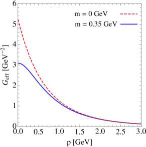
Figure 1: Effective two-body coupling as a function of $p$, cf. Eq. (16). We display the result for zero (dashed red) and finite (solid blue) dynamical quark masses. We have used the values $G_{q}=5.22\,\textrm{GeV}^{-2}$, $\lambda=0.65\,\textrm{GeV}$ and $q=1.103$.

2.2 The fractal NJL model

In order to introduce the fractal structure that emerges from the scaling properties associated to the renormalization of QCD, we implement a running coupling of Eq. (1) which is a direct consequence of the fractal structure [25, 26]. Therefore, the effects of the fractal structure can be implemented by substituting the constant coupling $G$ of the NJL model by the fractal running-coupling in the gap equation.

If we consider that one of the particles has zero energy, the effective two-body coupling can be written as

$$G_{\rm eff}(p~{};~{}G_{q},~{}\lambda~{},~{}q)=G_{q}\cdot\left[1+(q-1)\frac{\sqrt{p^{2}+m^{2}}}{\lambda}\right]^{-\frac{1}{q-1}}\;,$$ (16)

where we identify $G_{q}$ as the strength of the coupling. The behavior of $G_{\rm eff}(p)$ is displayed in Fig. 1, where we observe that the coupling decreases and approaches zero asymptotically. This is in clear contrast with the constant coupling, $G$, of the standard NJL model. In Fig. 1 we display the effective coupling in two cases: the chiral limit ($m=0$) and with broken chiral symmetry using $m=0.35$ GeV. In both cases, the effective coupling asymptotically approaches zero when the momentum goes to infinity. Then, the effective coupling eliminates the divergences and regularizes the fractal NJL model.

After the introduction of the running-coupling, the gap equation then reads

$$m=m_{0}+\frac{4mN_{c}N_{f}}{2\pi^{2}}\int_{0}^{\infty}dp\,p^{2}\frac{G_{\rm eff}(p)}{\sqrt{p^{2}+m^{2}}}\;,$$ (17)

for the case where $q>1$. The parameter $\lambda$ in the $q$-exponential function of Eq. (16) plays the role of a smooth cut-off. Notice that the integrand of Eq. (17) behaves as $\propto p^{1-\frac{1}{q-1}}$ at large momentum, so that the integral is convergent in the UV only if $q<3/2$. For the case $q<1$, the integration in momentum should be performed in the finite interval

$$0<p<\sqrt{\left(\frac{\lambda}{1-q}\right)^{2}-m^{2}}\;.$$ (18)

The upper limit corresponds to the momentum at which the $q$-exponential function vanishes. Then the integral in Eq. (17) is convergent also for $q<1$.

While the coupling of Eq. (16) plays the role of a regulator, it is important to stress at this point that beyond phenomenological considerations, this regulator has a physical motivation based on the thermofractal approach to QCD. Let us mention that it has been introduced in the literature other regulators that are connected to non-local interactions, see e.g. Refs. [34, 35].

In the fNJL model, the critical coupling in the chiral symmetric regime, $m_{0}=0$, is

$$\qquad G_{q,{\textrm{crit}}}=\frac{\pi^{2}}{2N_{c}N_{f}}\frac{(2-q)(3-2q)}{\lambda^{2}}\,,\qquad(0<q<3/2)\,.$$ (19)

For the sake of comparison, in the following we will compare the behaviour of some quantities in the NJL and in the fNJL models. For this comparison, we choose the parameter $\lambda$ in such a way that the critical point for both models coincide, that is, $G_{\textrm{crit}}=G_{q,\textrm{crit}}$. This leads to the following relation between the cut-offs

$$\lambda=\Lambda\sqrt{\frac{(2-q)(3-2q)}{2}}\,.$$ (20)

Notice that one has $\lambda=\Lambda/\sqrt{2}$ for $q=1$. More generally Eq. (20) implies $\lambda<\Lambda$ for $0.72<q<3/2$.

With this choice of parameters, we obtain the results in Fig. 2.

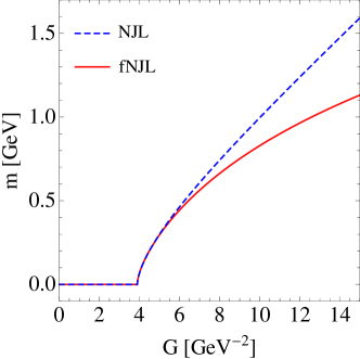
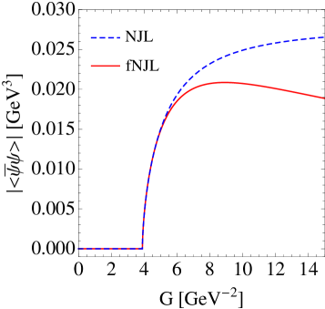
Figure 2: Gap mass (left panel) and condensate (right panel) as a function of the coupling. The critical value of $G$ is the same in both models: $G_{\textrm{crit}}=3.89\,\textrm{GeV}^{-2}$. This is obtained with $\Lambda=0.65\,\textrm{GeV}$ and $\lambda=0.388\,\textrm{GeV}$. Here we have considered $q=1.103$ and $m_{0}=0$. Note that both models match up to $G\approx 6~{}{\rm GeV}^{-2}$. The label $G$ refers either to the coupling $G$ for the NJL model, or $G_{q}$ for the fNJL model.

We observe that the behaviour of the mass gap, $m$, and the condensate $\langle\bar{\psi}\psi\rangle$ for both models are similar near the critical point for the choice of parameters we used. Therefore, despite the large differences in the couplings used in the two models, the results are similar in a wide range. The physical value for the pion mass is obtained by both the NJL and the fNJL models for similar values of the couplings. This result is obtained because the running-coupling of the fNJL model decreases fast near the value of the cut-off momentum.

It is important to stress that the use of the fractal inspired coupling leads to a $q$-exponential running coupling which renormalizes the gap equation. In Ref. [36], a qNJL model was proposed through a statistical approach, where the Tsallis entropy [30] was used in Eq. (5) to extend the NJL model. Here we adopted a different approach, using the dynamical aspects of the QCD incorporating the fractal structure through the effective coupling. This approach leads to a nonextensive version of the NJL model as well. It would be interesting to study the similarities between the qNJL model from Ref. [36] and the fNJL model proposed here. However, in the present work we will follow a different path. Since our approach allows us to connect the entropic index, $q$, to the fundamental parameters of the QFT, as the number of flavours and colours in QCD, we will investigate the behaviour of the fNJL model when the parameter $q$ changes, and then we will associate this to different QFTs, where the number of flavours and colours may differ from those of the QCD. The model presented in Ref. [36] was extended to include the Polyakov loop (qPNJL) [37], and the use of the fractal-inspired coupling adopted here can be easily applied to the qPNJL model as well. A more detailed comparison between the present model and those proposed in Refs. [36, 37] will be presented elsewhere.

2.3 Behaviour of the fractal NJL model

The fNJL model will present some advantages if it can go beyond the standard NJL model. To verify how it behaves in different conditions, we now look for the parameters that reproduce the values of some important physical quantities. Here, we use the pions mass and the GOR relation as the physical quantities to fix the parameters of the fNJL model. The assumption that the physical values of $m_{\pi}$ and $f_{\pi}$ are reproduced in both models, does not lead necessarily to the same critical values for the couplings. In fact, by using the expressions of Eqs. (10) and (19) we get

$$\frac{G_{q,\textrm{crit}}}{G_{\textrm{crit}}}=\frac{1}{2}(2-q)(3-2q)\left(\frac{\Lambda}{\lambda}\right)^{2}\,.$$ (21)

This formula implies that $G_{q,{\textrm{crit}}}<G_{{\textrm{crit}}}$ for $\lambda\simeq\Lambda$ and $0.72<q<3/2$.

In the pursuit for the values of the fNJL parameters that allow to reproduce the physical quantities, we use the NJL model as a guide. We calculate the condensate density using the NJL model with the parameters with which the model reproduces the physical values for the pion mass and its decay width, and then find the best values for $G_{q}$, $\lambda$ and $q$ that reproduce the same condensate density.

The condensate density can be calculated analytically in the asymptotic regime $m\gg\lambda$ for any values of $0<q<3/2$. The asymptotic expression is

$$\langle\bar{\psi}\psi\rangle\stackbin[G_{q}\gg 1/\lambda^{2}]{\simeq}{}\left\{\begin{array}[]{cl}&-2^{-\frac{2-q}{3-2q}}\pi^{-\frac{3}{2}\frac{q-1}{3-2q}}N_{c}^{\frac{q-1}{3-2q}}(N_{f}G_{q})^{\frac{3q-4}{3-2q}}\left(\frac{\lambda}{q-1}\right)^{\frac{1}{3-2q}}\left(\frac{\Gamma\left[\frac{3-2q}{2(q-1)}\right]}{\Gamma\left[\frac{q}{2(q-1)}\right]}\right)^{\frac{q-1}{3-2q}}\,;\qquad~{}~{}~{}1<q<3/2\\ &-\frac{\lambda}{2N_{f}G_{q}}\log\left(\frac{N_{c}N_{f}}{\pi^{3/2}}G_{q}\lambda^{2}\right)\,;\qquad\qquad~{}~{}~{}~{}~{}~{}~{}~{}~{}~{}~{}~{}~{}~{}~{}~{}~{}~{}~{}~{}~{}~{}~{}\qquad\qquad\qquad\qquad q=1\\ &\frac{1}{2N_{f}G_{q}}\left[-\left(\frac{\lambda}{1-q}\right)+\left(\frac{\pi^{3}}{2N_{c}^{2}N_{f}^{2}G_{q}^{2}}\right)^{\frac{1-q}{5-3q}}\left(\frac{\lambda}{1-q}\right)^{\frac{1+q}{5-3q}}\left(\frac{\Gamma\left[\frac{7-5q}{2(1-q)}\right]}{\Gamma\left[\frac{2-q}{1-q}\right]}\right)^{\frac{2(1-q)}{5-3q}}\right]\,;\qquad q<1\end{array}\,.\right.$$ (22)

At large value of the coupling the chiral condensate presents a power-law behaviour $\langle\bar{\psi}\psi\rangle\propto G_{q}^{\frac{3q-4}{3-2q}}\;(1<q<3/2)$, $\langle\bar{\psi}\psi\rangle\propto 1/G_{q}\;(q<1)$ and $\langle\bar{\psi}\psi\rangle\propto\log(G_{q})/G_{q}\;(q=1)$. It turns out that in the large coupling limit the chiral condensate tends to zero for $q<4/3$, while it tends to infinity for $4/3<q<3/2$. The value $q=3/2$ was found to be a limit for a physical system condensate [38]. In the critical case $q=4/3$, the chiral condensate tends to the constant value

$$\langle\bar{\psi}\psi\rangle\stackbin[G_{q}\to\infty]{\longrightarrow}{}-\frac{27N_{c}}{4\pi}\lambda^{3}\,.$$ (23)

The chiral condensate in the NJL model also tends to a constant value in this limit, cf. Eq. (11). We display in the left panel of Fig. 3 the behavior of $|\langle\bar{\psi}\psi\rangle|$ in the NJL and fNJL models up to $G=100\,\textrm{GeV}^{-2}$. Note that, in the range $1<q<4/3$, even though the condensate decreases as $G_{q}$ increases, the product $G_{q}\langle\bar{\psi}\psi\rangle$ is still increasing with $G_{q}$. From Eq. (4), we conclude that the dynamical mass, $m$, also increases with $G_{q}$. The physical interpretation of this result is the following: for the parameter $q$ in that range, the effective coupling decreases very fast with $p$, then the contribution of the high momentum components of the pair to the effective mass is small, and only less energetic contributions to the self-energy are relevant. This effect is illustrated in the right panel of Fig. 3, where it has been displayed the behavior of $G_{\rm eff}(p)$ for several values of the parameter $q$. Thus, the condensate is restricted to quarks with small momenta, and high-momentum bound pairs cannot be formed. The effects of this behaviour of the fNJL model will be discussed in more detail below.

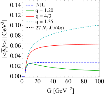
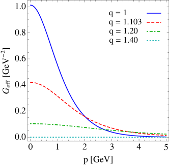
Figure 3: Left panel: Condensate as a function of the coupling up to $G=100\,\textrm{GeV}^{-2}$. The horizontal dotted line corresponds to the asymptotic limit of $|\langle\bar{\psi}\psi\rangle|$ in the fNJL model for $q=4/3$. We have considered $\Lambda=0.65\,\textrm{GeV}$ and $m_{0}=0$. The values of $\lambda$ are obtained for each curve by using Eq. (20). Right panel: Effective two-body coupling as a function of $p$, cf. Eq. (16). We display the results for several values of $q$: $q=1,1.103,1.20$ and $1.40$. The dynamical mass, $m$, is obtained for each value of $q$ from the solution of the gap equation, Eq. (17). In this panel, we have used the values $G_{q}=5.22\,\textrm{GeV}^{-2}$, $\lambda=0.65\,\textrm{GeV}$and $m_{0}=0$.

In Fig. 4 top left panel we show the behaviour of the condensate density obtained through the fNJL model as a function of $G_{q}$ (as a function of $G$ for the NJL model) for different values of the parameter $q$, in the regime of the transition between the Wigner-Weyl and Nambu-Goldstone phases. Observe that the critical point for the extended model is practically coincident with that for the standard NJL model, as all curves almost coincide up to $G_{q}\sim 4.5\,\textrm{GeV}^{-2}$ . Above this value, the curves present different behaviours showing a clear dependence on the value for $q$, and they cross the NJL condensate value at different points. As the value for $q$ increases, the crossing point approaches that of the NJL model. In Fig. 4 top right panel we see the behaviour of values for $q$ in the fNJL model that results in the same condensate value obtained by the standard NJL model, that is, the point where the curves cross the horizontal line in the top left panel of the same figure. We observe that only for $q=1.125$ the condensate will be the same for the two models for $\Lambda=0.65\,\textrm{GeV}$ and for the same values of the couplings, i.e. $G=G_{q}$. In the following we will denote by $q_{\textrm{match}}$ the value of $q$ the leads to the same values of the couplings, so that $q_{\textrm{match}}(\Lambda)|_{\Lambda=0.65\,\textrm{GeV}}=1.125$.

As discussed previously, the fractal model prediction is of $q=1.103$ for $N_{f}=2$, so we have to change the other parameters in order to obtain the same condensate density in both models when the expected value for $q$ is used, that is, we will fix the value for $q$ and change the other parameters of the model. We have checked that the value for $q_{\textrm{match}}$ is practically independent of $m_{0}$, so we keep it fixed at $m_{0}=5.0$ MeV. The dependence of $q_{\textrm{match}}$ with the parameter $\Lambda$, where the relation between $\lambda$ and $\Lambda$ given by Eq. (20) is considered, is displayed in the bottom left panel of Fig. 4. From there we get the value $\Lambda=0.719\,\textrm{GeV}$ that returns the same value of the condensate for both models in the case $q_{\textrm{match}}=1.103$. Therefore, the fNJL model is able to reproduce the condensate value given by the NJL model with the correct value for $q$ calculated according to the fractal approach to QCD.

Since we modified the value for $\Lambda$ in the NJL model, we had to recalculate the coupling $G$ that would give the correct physical value for the quark condensate. The behaviour of $G$ with $\Lambda$ in the NJL model is shown in the bottom right panel of Fig. 4. From this plot we get the value $G_{\textrm{Phys}}=3.703\,\textrm{GeV}^{-2}$.

With the method just described, we reproduce the condensate value of the NJL model by using the fNJL model with the parameter $q=1.103$ determined by the fractal approach. We summarize the values for the parameters in Table 1. In the following subsection we will describe how the pion mass and pion decay constant, which are physical quantities, are determined in the fNJL model.

parameter	NJL	fNJL
$\Lambda\;|\;\lambda$         [GeV]	0.719	0.429
$G\;|\;G_{q}$        [GeV-2]	3.703	3.703
$G_{\textrm{crit}}\;|\;G_{q,\textrm{crit}}$   [GeV-2]	3.185	3.185
$q$	-	1.103

Table 1: Table of parameters for the NJL and fNJL models that reproduce the same value for the quark condensate $\langle\bar{\psi}\psi\rangle_{\textrm{Phys}}=-(0.255\,\textrm{GeV})^{3}$ with the condition $G_{\textrm{crit}}=G_{q,\textrm{crit}}$, for $m_{0}=5\,\textrm{MeV}$.

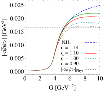
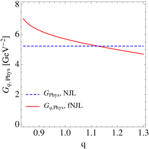
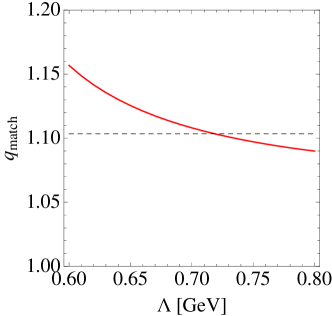
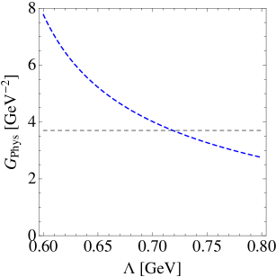
Figure 4: Upper left panel: Condensate as a function of the coupling for $m_{0}=5.0\,\textrm{MeV}$. The horizontal dotted line corresponds to the physical value of $|\langle\bar{\psi}\psi\rangle|$ given by Eq. (14). Upper right panel: Physical value of $G_{q}$ as a function of $q$ (red line) for $\Lambda=0.65\,\textrm{GeV}$. We display also the physical value for the NJL model, which is $G=5.22\,\textrm{GeV}^{-2}$ (dashed blue line). The physical values of $G$ and $G_{q}$ correspond to the intersection of the horizontal line with each curve in the left panel. The matching between the NJL and fNJL results happens at $q_{\textrm{match}}=1.125$ for $\Lambda=0.65\,\textrm{GeV}$. Lower left panel: $q_{\textrm{match}}$ as a function of $\Lambda$. To guide the eye we have displayed as an horizontal dashed line the value $q=1.103$, which is obtained for $\Lambda=0.719\,\textrm{GeV}$. Lower right panel: $G_{\textrm{Phys}}$ as a function of $\Lambda$ for the NJL model. The horizontal dashed line corresponds to the value $G_{\textrm{Phys}}=3.703\,\textrm{GeV}^{-2}$, which crosses the dashed blue curve at $\Lambda=0.719\,\textrm{GeV}$.

2.4 Reproducing the pion mass and the pion decay constant

We proceed investigating the results of the fNJL model for the physical parameters, namely, the pions mass and the pions decay constant.

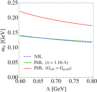
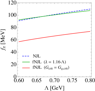
Figure 5: Left panel: Pion mass $m_{\pi}$ as a function of the cut-off $\Lambda$ as given by Eq. (26). Right panel: Pion decay constant $f_{\pi}$ as a function of $\Lambda$. The results for the fNJL model have been obtained in two different scenarios: A) for $G_{\textrm{crit}}=G_{q,\textrm{crit}}$ at the matching point $q=q_{\textrm{match}}(\Lambda)$, with the relation between $\lambda$ and $\Lambda$ given by Eq. (20) (red line); and B) for $\lambda=1.16\Lambda$ (green line). We have considered $q=1.103$ in scenario B, and fixed values of $m=0.35\,\textrm{GeV}$ and $m_{0}=5\,\textrm{MeV}$ in both panels.

The pion mass is obtained from the pole of the T-matrix, by the condition [6]

$$1-2GJ_{\pi}(q^{2}=m_{\pi}^{2})=0\,,$$ (24)

where

$$J_{\pi}(q^{2})=i\textrm{Tr}\int\frac{d^{4}p}{(2\pi)^{4}}\left[i\gamma_{5}\frac{1}{/{\!\!\!p}+\frac{/{\!\!\!q}}{2}-m+i\epsilon}i\gamma_{5}\frac{1}{/{\!\!\!p}-\frac{/{\!\!\!q}}{2}-m+i\epsilon}\right]\,.$$ (25)

Then, the result for the pion mass is obtained as the solution of the equation [18]

$$m_{\pi}^{2}=-\frac{m_{0}}{m}\frac{1}{4iGN_{c}N_{f}I(m_{\pi}^{2})}\,,$$ (26)

where $I$ is a function which reads

$$I_{\textrm{NJL}}(k^{2})=\frac{i}{8\pi^{2}}\int_{0}^{1}dx\int_{0}^{\Lambda}dp\frac{p^{2}}{\left(p^{2}+\bar{m}^{2}(k^{2})\right)^{3/2}}=\frac{i}{8\pi^{2}}\int_{0}^{1}dx\left[\sinh^{-1}\left(\frac{\Lambda}{\bar{m}(k^{2})}\right)-\frac{\Lambda}{\sqrt{\Lambda^{2}+\bar{m}^{2}(k^{2})}}\right]\,,$$ (27)

in the NJL model, and

$$I_{\textrm{fNJL}}(k^{2})=\frac{i}{8\pi^{2}}\int_{0}^{1}dx\int_{0}^{\infty}dp\frac{p^{2}}{\left(p^{2}+\bar{m}^{2}(k^{2})\right)^{3/2}}\left[1+(q-1)\frac{\sqrt{p^{2}+\bar{m}^{2}(k^{2})}}{\lambda}\right]^{-\frac{1}{q-1}}\,,$$ (28)

in the fNJL model. In these expressions

$$\bar{m}^{2}(k^{2})=m^{2}-x(1-x)k^{2}\,.$$ (29)

The other observable that can be calculated is the pion decay constant. The quantity is computed in the NJL model as

$$f^{2}_{\pi,\textrm{NJL}}=\frac{N_{c}m^{2}}{2\pi^{2}}\int_{0}^{\Lambda}dp\frac{p^{2}}{\left(p^{2}+m^{2}\right)^{3/2}}=\frac{N_{c}m^{2}}{2\pi^{2}}\left[\log\left(x+\sqrt{1+x^{2}}\right)-\frac{x}{\sqrt{1+x^{2}}}\right]\,,\qquad x\equiv\frac{\Lambda}{m}\,,$$ (30)

while it is computed in the fNJL model as

$$f^{2}_{\pi,\textrm{fNJL}}=\frac{N_{c}m^{2}}{2\pi^{2}}\int_{0}^{\infty}dp\frac{p^{2}}{\left(p^{2}+m^{2}\right)^{3/2}}\left[1+(q-1)\frac{\sqrt{p^{2}+m^{2}}}{\lambda}\right]^{-\frac{1}{q-1}}\,.$$ (31)

Notice that the integrands of Eqs. (28) and (31) behave as $\propto p^{-1-\frac{1}{q-1}}$ at large momentum, so that the corresponding integrals are convergent in the UV for any value of $q>1$. For the case $q<1$, the integrations should be performed in the finite interval in momentum provided in Eq. (18), leading thus also to convergent results.

We will consider the computation of the pion mass and the pion decay constant within the fNJL model in two different scenarios: scenario A) where the critical values of the couplings, $G_{\textrm{crit}}$ and $G_{q,\textrm{crit}}$, for the NJL and fNJL model coincide, and scenario B) where the values of the cut-off are close each other, $\lambda\simeq\Lambda$. The first scenario corresponds to assuming the relation between $\lambda$ and $\Lambda$ given by Eq. (20). We will assume in both scenarios a fixed value for the dynamical quark mass, $m=0.35\,\textrm{GeV}$, and coupling constants, $G=G_{q}=5.22\,\textrm{GeV}^{-2}$, and study the dependence of the observables with the cut-off $\Lambda$.

In Fig. 5 we plot the value of the pion mass (left panel) and pion decay constant (right panel) as a function of the parameter $\Lambda$, obtained with the two models. The scenario A leads to a disagreement between the models, and in this situation the fNJL model cannot reproduce simultaneously the pion mass and pion decay constant. On the contrary, in scenario B, when using $\lambda=1.16\Lambda$, there is a good agreement between the two models, and the physical values for both the pion mass and pion decay constant are correctly predicted. In this scenario, both models lead to very similar values of $m_{\pi}$ and $f_{\pi}$ in the full range of the figure: $0.6\,\textrm{GeV}\leq\Lambda\leq 0.8\,\textrm{GeV}$.

In the left hand panel of Fig. 6, we plot the condensate density for the NJL model and for the fNJL model for fixed value of $\Lambda=0.65\,\textrm{GeV}$, in the two scenarios discussed above. For scenario B, the condensate density is larger than that obtained in the NJL model for all values of the coupling, while for the scenario A the condensate for the NJL and for the fNJL model are similar. It is possible to observe that the critical coupling for scenario B (i.e. when $\lambda\simeq\Lambda$) is considerably smaller than that for the NJL model. For scenario A, the critical couplings are the same by construction.

One of the strengths of the NJL model is the fact that it satisfies the GOR relation, given by Eq. (12). This relation is based on general aspects of the SU(2) symmetry, and thus represents fundamental properties of the hadron structure at low energies. It relates the hadron mass and its decay constant to the parton bare mass and to the condensate density. Aside from the pion mass and pion decay constant, we can use the GOR relation to check the quality of the results obtained here. The results of the GOR relation for both models are displayed in the right hand panel of Fig. 6. We observe that, despite the different condensate densities, the NJL model and the fNJL model with $\lambda=1.16\Lambda$ equally satisfy the GOR relation in a wide range of $\Lambda$. The fNJL model in scenario A, on the other hand, cannot satisfy that relation. This is a consequence of the fact that in this scenario the model cannot reproduce simultaneously the physical pion mass and pion decay constant.

Although the fNJL model, with appropriate parameters, gives the correct pion mass and pion decay constant, we have seen that the condensate density presents a behaviour that is different from that obtained in the standard NJL model as a function of the coupling. Aside the different critical couplings, the behaviour of the condensate with the interaction strength is different, increasing faster than in the NJL model in the region around the critical value. Also, we observe a saturation of the condensate, resulting in a peak around $G_{q}\sim 2~{}\textrm{GeV}^{-2}$, followed by a monotonic decrease. It means that there are two possible values for the coupling that results in the same value for the condensate density. The pion mass, however, always decreases with the coupling strength, so only one value of the coupling will result in the physical pion.

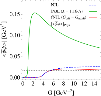
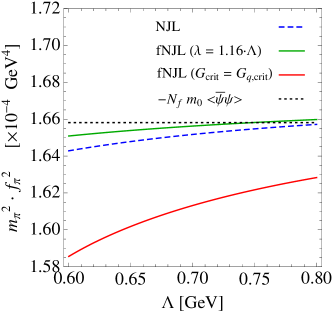
Figure 6: Left panel: Condensate as a function of the coupling for fixed value of $\Lambda=0.65\,\textrm{GeV}$. Right panel: Check of the GOR relation. In both panels we display the results for the NJL model, and for the fNJL model considering scenarios A and B. See caption of Fig. 5 for details.

3 Conclusions and outlook

In this work we have studied the generalization of the NJL model by the inclusion of an effective coupling inspired in the fractal structure of the Yang-Mills fields. The running coupling constant works as a natural regularization method for the theory, eliminating the divergences that are present in the standard NJL model.

We study the generalized model in two scenarios, one that reproduces the same critical coupling as the standard NJL model, and other that reproduces the pion mass and the pion decay constant simultaneously. We show that the first scenario does not satisfy the GOR relation, while the second one satisfies that relation in the same way as the NJL model.

The physical scenario for the fNJL model results in a different behavior of the condensate, resulting in a different critical coupling with respect to the NJL model. Also, the physical coupling, that reproduces the pion properties, is smaller than that of the NJL model, and closer to the critical value than what is observed in the NJL model.

Since the running coupling constant used is inspired in the fractal approach used in HEP to study the multi particle production in high energy collisions, the generalization of the NJL model presented here allows to connect the hadron structure properties to the properties of the hot and dense matter obtained in those collisions. This model opens the possibility to study, in a unified way, the QCD properties in the high energy limit and in the low energy limit of the hadron structure. This unified procedure counts with the consistent fractal approach to the QCD that results in the fractal-inspired effective coupling.

We have seen that in the range $1<q<4/3$, an interesting phenomenon takes place: while the condensate density decreases, the hadron mas still increases with the coupling strength. By using Eqs. (2) and (22), one can see that the behavior of $\langle\bar{\psi}\psi\rangle\stackbin[G_{q}\to\infty]{\longrightarrow}{}0$ in the fNJL model, which corresponds to $q<4/3$, is obtained for

$$N_{f}<\frac{1}{2}\left(11N_{c}-9\right)\,,$$ (32)

while values of $N_{f}$ larger than that lead to $\langle\bar{\psi}\psi\rangle\stackbin[G_{q}\to\infty]{\longrightarrow}{}\infty$. Then, for $N_{c}=3$ a vanishing value of the chiral condensate in the large coupling limit is obtained for $N_{f}<12$, while in the case $N_{c}=1=N_{f}$ the fNJL model would be in the critical situation $q=4/3$.

For any non Abelian field theory with $N_{f}$ in agreement with the relation (32), only the pairs quark/anti-quark with low momenta would condensate, but the hadron mass would, nevertheless, increase. In a field theory with the structure parameters in the range above, we would have massive partons but no condensate for very large couplings. In this case, we can conjecture that there would be no formation of a system similar to the QGP, and the high energy processes would result in the direct production of particles. The coalescence mechanism would be less important, and the particle multiplicity would be higher, and with more massive particles.

This mechanism might be the responsible for production of dark-matter, in particular it could constitute a mechanism of dark-matter formation based on the sector of the non-Abelian Yang-Mills theory.

The model introduced here opens the possibility to investigate new aspects of the hadronic matter near the transition between the Wigner-Weyl and the Nambu-Goldstone phases. In particular, the role of the different flavours and their masses, or the effective number of flavours in the formation of the condensate. The model allows to study how the critical value, or its existence, depends on the number of colours and flavours.

References

- [1] R. Hagedorn, “How We Got to QCD Matter from the Hadron Side: 1984,” Lect. Notes Phys., vol. 221, pp. 53–76, 1985.
- [2] N. O. Agasian, “Nonperturbative vacuum and condensates in QCD below thermal phase transition,” Phys. Lett. B, vol. 519, pp. 71–77, 2001.
- [3] E. Megías, E. Ruiz Arriola, and L. L. Salcedo, “The Polyakov loop and the hadron resonance gas model,” Phys. Rev. Lett., vol. 109, p. 151601, 2012.
- [4] Y. Nambu and G. Jona-Lasinio, “Dynamical model of elementary particles based on an analogy with superconductivity. i.,” Physical Review, vol. 122, pp. 345–358, 1961.
- [5] Y. Nambu and G. Jona-Lasinio, “Dynamical model of elementary particles based on an analogy with superconductivity. ii.,” Physical Review, vol. 124, pp. 246–254, 1961.
- [6] U. Vogl and W. Weise, “The Nambu and Jona Lasinio model: Its implications for hadrons and nuclei,” Prog. Part. Nucl. Phys., vol. 27, pp. 195–272, 1991.
- [7] S. P. Klevansky, “The Nambu-Jona-Lasinio model of quantum chromodynamics,” Rev. Mod. Phys., vol. 64, pp. 649–708, 1992.
- [8] M. Buballa, “NJL model analysis of quark matter at large density,” Phys. Rept., vol. 407, pp. 205–376, 2005.
- [9] K. Fukushima, “Chiral effective model with the Polyakov loop,” Phys. Lett. B, vol. 591, pp. 277–284, 2004.
- [10] C. Ratti, M. A. Thaler, and W. Weise, “Phases of QCD: Lattice thermodynamics and a field theoretical model,” Phys. Rev. D, vol. 73, p. 014019, 2006.
- [11] E. Megías, E. Ruiz Arriola, and L. L. Salcedo, “Polyakov loop in chiral quark models at finite temperature,” Phys. Rev. D, vol. 74, p. 065005, 2006.
- [12] E. Megías, E. Ruiz Arriola, and L. L. Salcedo, “Chiral Lagrangian at finite temperature from the Polyakov-Chiral Quark Model,” Phys. Rev. D, vol. 74, p. 114014, 2006.
- [13] S. Roessner, C. Ratti, and W. Weise, “Polyakov loop, diquarks and the two-flavour phase diagram,” Phys. Rev. D, vol. 75, p. 034007, 2007.
- [14] M. Ferreira, P. Costa, D. P. Menezes, C. Providência, and N. Scoccola, “Deconfinement and chiral restoration within the SU(3) Polyakov–Nambu–Jona-Lasinio and entangled Polyakov–Nambu–Jona-Lasinio models in an external magnetic field,” Phys. Rev. D, vol. 89, no. 1, p. 016002, 2014. [Addendum: Phys.Rev.D 89, 019902 (2014)].
- [15] R. L. S. Farias, K. P. Gomes, G. Krein, and M. B. Pinto, “The role of asymptotic freedom for the pseudocritical temperature in magnetized quark matter,” J. Phys. Conf. Ser., vol. 630, no. 1, p. 012046, 2015.
- [16] V. P. Pagura, D. Gomez Dumm, S. Noguera, and N. N. Scoccola, “Magnetic catalysis and inverse magnetic catalysis in nonlocal chiral quark models,” Phys. Rev. D, vol. 95, no. 3, p. 034013, 2017.
- [17] R. L. S. Farias, V. S. Timóteo, S. S. Avancini, M. B. Pinto, and G. Krein, “Thermo-magnetic effects in quark matter: Nambu–Jona-Lasinio model constrained by lattice QCD,” Eur. Phys. J. A, vol. 53, no. 5, p. 101, 2017.
- [18] S. S. Avancini, R. L. S. Farias, M. Benghi Pinto, W. R. Tavares, and V. S. Timóteo, “ pole mass calculation in a strong magnetic field and lattice constraints,” Phys. Lett. B, vol. 767, pp. 247–252, 2017.
- [19] M. Coppola, D. Gómez Dumm, and N. N. Scoccola, “Charged pion masses under strong magnetic fields in the NJL model,” Phys. Lett. B, vol. 782, pp. 155–161, 2018.
- [20] W. R. Tavares, R. L. S. Farias, and S. S. Avancini, “Deconfinement and chiral phase transitions in quark matter with a strong electric field,” Phys. Rev. D, vol. 101, no. 1, p. 016017, 2020.
- [21] A. Ayala, R. L. S. Farias, S. Hernández-Ortiz, L. A. Hernández, D. M. Paret, and R. Zamora, “Magnetic field-dependence of the neutral pion mass in the linear sigma model coupled to quarks: The weak field case,” Phys. Rev. D, vol. 98, no. 11, p. 114008, 2018.
- [22] S. S. Avancini, V. Dexheimer, R. L. S. Farias, and V. S. Timóteo, “Anisotropy in the equation of state of strongly magnetized quark matter within the Nambu–Jona-Lasinio model,” Phys. Rev. C, vol. 97, no. 3, p. 035207, 2018.
- [23] C. G. Callan Jr, “Broken scale invariance in scalar field theory,” Physical Review D, vol. 2, no. 8, p. 1541, 1970.
- [24] K. Symanzik, “Small distance behaviour in field theory and power counting,” Communications in Mathematical Physics, vol. 18, no. 3, pp. 227–246, 1970.
- [25] A. Deppman, “Thermodynamics with fractal structure, Tsallis statistics and hadrons,” Phys. Rev. D, vol. 93, p. 054001, 2016.
- [26] A. Deppman, T. Frederico, E. Megías, and D. P. Menezes, “Fractal structure and non-extensive statistics,” Entropy, vol. 20, no. 9, p. 633, 2018.
- [27] R. Hagedorn, “Statistical thermodynamics of strong interactions at high energies,” Nuovo Cimento, Suppl., vol. 3, no. CERN-TH-520, pp. 147–186, 1965.
- [28] G. F. Chew and A. Pignotti, “Multiperipheral bootstrap model,” Physical Review, vol. 176, no. 5, p. 2112, 1968.
- [29] S. Frautschi, “Statistical bootstrap model of hadrons,” Physical Review D, vol. 3, no. 11, p. 2821, 1971.
- [30] C. Tsallis, “Possible Generalization of Boltzmann-Gibbs Statistics,” J. Statist. Phys., vol. 52, pp. 479–487, 1988.
- [31] A. Deppman, “Self-consistency in non-extensive thermodynamics of highly excited hadronic states,” Physica A - Statistical Mechanics and Its Applications, vol. 391, no. 24, pp. 6380–6385, 2012.
- [32] A. Deppman, E. Megías, and D. P. Menezes, “Fractals, nonextensive statistics, and QCD,” Phys. Rev. D, vol. 101, no. 3, p. 034019, 2020.
- [33] M. Gell-Mann, R. J. Oakes, and B. Renner, “Behavior of current divergences under SU(3) x SU(3),” Phys. Rev., vol. 175, pp. 2195–2199, 1968.
- [34] D. Gomez Dumm and N. N. Scoccola, “Chiral quark models with nonlocal separable interactions at finite temperature and chemical potential,” Phys. Rev. D, vol. 65, p. 074021, 2002.
- [35] G. A. Contrera, D. G. Dumm, and N. N. Scoccola, “Meson properties at finite temperature in a three flavor nonlocal chiral quark model with Polyakov loop,” Phys. Rev. D, vol. 81, p. 054005, 2010.
- [36] J. Rożynek and G. Wilk, “Nonextensive Nambu-Jona-Lasinio Model of QCD matter,” Eur. Phys. J. A, vol. 52, no. 1, p. 13, 2016. [Erratum: Eur.Phys.J.A 52, 204 (2016)].
- [37] Y.-P. Zhao, “Thermodynamic properties and transport coefficients of QCD matter within the nonextensive Polyakov–Nambu–Jona-Lasinio model,” Phys. Rev. D, vol. 101, no. 9, p. 096006, 2020.
- [38] E. Megías, V. S. Timóteo, A. Gammal, and A. Deppman, “Bose–Einstein condensation and non-extensive statistics for finite systems,” Physica A: Statistical Mechanics and its Applications, vol. 585, p. 126440, 2022.