White Dwarf Photospheric Abundances in Cataclysmic Variables - II. White Dwarfs With and Without a Mask

Abstract

Taking advantage of the now available Gaia EDR3 parallaxes, we carry out an archival Hubble Space Telescope (HST) far ultraviolet spectroscopic analysis of 10 cataclysmic variable systems, including 5 carefully selected eclipsing systems. We obtain accurate white dwarf (WD) masses and temperatures, in excellent agreement with the masses for 4 of the eclipsing systems. For three systems in our sample, BD Pav, HS 2214, and TT Crt, we report the first robust masses for their WDs. We modeled the absorption lines to derive the WD chemical abundances and rotational velocities for each of the ten systems. As expected, for five higher inclination ($i\gtrsim 75^{\circ}$) systems, the model fits are improved with the inclusion of a cold absorbing slab (an iron curtain masking the WD) with $N_{\rm H}\approx 10^{20}-10^{22}$cm^-2. Modeling of the metal lines in the HST spectra reveals that 7 of the 10 systems have significant subsolar carbon abundance, and six have subsolar silicon abundance, thereby providing further evidence that CV WDs exhibit subsolar abundances of carbon and silicon. We suggest that strong aluminum absorption lines (and iron absorption features) in the spectra of some CV WDs (such as IR Com) may be due to the presence of a thin iron curtain ($N_{\rm H}\approx 10^{19}$cm^-2) rather than to suprasolar aluminum and iron abundances in the WD photosphere. The derived WD (projected) rotational velocities all fall in the range $\approx 100-400$ km/s, all sub-Keplerian similar to the values obtained in earlier studies.

Arxiv Version 0.9in

1 Introduction

Cataclysmic variables (CVs) are compact binaries in which a white dwarf (WD) accretes matter and angular momentum from a main-sequence-like star. In nonmagnetic CVs, the matter is transferred, at continuous or sporadic rates, by means of an accretion disk around the WD. Dwarf novae (DNe; a class of nonmagnetic CVs) release gravitational energy when a thermal-viscous instability in the accretion disk around the WD leads to rapid accretion at a high rate (the dwarf nova outburst, lasting days to weeks) until the disk has largely emptied and the system returns to quiescence, at which time the buildup of disk gas begins again (lasting weeks to months). When a DN system is in quiescence, the WD is often revealed in the ultraviolet (UV), as its emission greatly outshines the disk (Warner, 1995; Frank et al., 2002).

Accretion is expected to spin up the WD envelope relative to the rotation of its core (Narayan & Popham, 1989), and over the lifetime of a CV (e.g. $\sim 10^{9}$yrs), the accretion of 0.1-0.2 $M_{\odot}$ of gas with angular momentum should spin up the CV WD to its critical breakup Keplerian rotational velocity (Livio & Pringle, 1998). Interestingly enough, however, most exposed CV WDs reveal a (projected) stellar rotation rate of only a fraction of the breakup velocity (usually 200-400 km/s, see e.g. Sion, 1998, 1999; Godon et al., 2012). The efficiency of the coupling between the core and envelope, however, remains poorly understood (Yoo & Langer, 2004). While nova explosions may spin down the rotation rates to well below the critical rotation, if the accretion rate is low and the WD of average or moderate mass, then the recurrence time between novae is longer and an accreting WD should possibly have a faster rotation rate than higher mass accreting WDs. Clearly, accurate WD stellar rotational velocities are required to achieve an understanding of CV evolution and spin-up of the WDs due to accretion with angular momentum.

On the other hand, the UV spectra of accreted material on the WD can be regarded as a mass spectrometer for revealing the composition of the donor and its evolutionary history. Suprasolar N/C ratio anomaly has been detected in some systems and it is estimated that at least 10 to 15% of CVs might have a suprasolar N/C ratio (Gänsicke et al., 2003, based on anomalous UV line flux ratios). Infrared analyses of CV secondary stars (e.g. Harrison et al., 2004, 2005; Howell et al., 2010) have further shown, based on depleted levels of ¹²C and enhanced levels of ¹³C, that material that has been processed in the CNO cycle is finding its way into the photospheres of secondary stars. One possible scenario is that the N/C overabundance anomaly arises from the donor star, a formerly more massive secondary donor star (capable of CNO burning) having been peeled away by mass transfer down to its CNO-processed core. An alternative explanation is that the anomaly originates in the WD itself due to explosive hot CNO burning associated with nova explosions. In that case, the N/C anomaly and suprasolar abundances of heavy elements could be due to the contamination of the donor star by nova explosion followed by re-accretion of this material by the WD (Sion & Sparks, 2014; Sparks & Sion, 2021).

Accurate CV WD masses have been needed to help answer fundamental questions in CV evolution theories, such as whether a CV WD mass can grow, reach the Chandrasekhar limit, and explode as a supernova (SN) Ia; or which of the different CV evolution theories based on different (binary) angular momentum braking laws is correct (Schreiber et al., 2016; Nelemans et al., 2016; Lauffer et al., 2018; McAllister et al., 2019; Zorotovic et al., 2020). However, knowing the mass and temperature of a WD is also needed to derive the WD surface chemical abundances and (projected) stellar rotational velocities. This is because the shape and depth of absorption lines in UV spectra depend, not only on the chemical abundances and rotational velocity, but also on the temperature and gravity of the WD stellar photosphere. Consequently, in order to derive chemical abundances and rotational velocities one has to first derive the WD surface temperature and mass.

With the era of space UV telescopes, and in particular with the International Ultraviolet Explorer (IUE), the Far Ultraviolet Spectroscopic Explorer (FUSE), and the Hubble Space Telescope (HST), significant advances have been made in the the field of CVs (see e.g. La Dous, 1991; Hack & La Dous, 1993; Warner, 1995). Thanks to recent Gaia eDR3 parallaxes (Brown et al., 2021), further progress can now be made to fully exploit the large number of available far-UV (FUV, $\lambda<2000$ Å) spectra of CVs (see, e.g. the current FUV spectral analysis of Pala et al., 2021). Scaled to the Gaia distances, model spectra can provide accurate temperature, WD radius/masses, as well as accurate WD photospheric abundances and rotational velocities for a large number of CV WDs.

Up to now, there are only 5 systems (all DNe) in which detections of suprasolar heavy element abundances are manifested by FUV photospheric absorption line in the spectra of CV WDs exposed during DN quiescence (Long & Gilliland, 1999; Gänsicke et al., 2005). All five CV WDs have suprasolar abundances of nuclides like Al with atomic masses A$>$20. The best studied systems are U Gem (Sion et al., 1998; Long & Gilliland, 1999; Godon et al., 2017) and VW Hyi (Sion et al., 1995a, b, 1997; Long et al., 2006, 2009). U Gem WD after an outburst and into mid-quiescence has abundances C$\approx$0.30 - 0.35, N$\approx$35 - 41, and Si$\approx$1.4 - 4, S$\approx$6.6 - 10 (Long & Gilliland, 1999). In quiescence subsolar to solar abundances of C and S were found, together with suprasolar abundance of N and Al (both up to 20 solar) and subsolar to suprasolar abundances of Si (Godon et al., 2017). For VW Hyi, subsolar (0.4-0.8) abundance of carbon was found with suprasolar abundance of N (4-6) and Si (2.5-4.4) and about solar abundance of S (with rotational velocity on the higher side: 400-570 km/s). In three SU UMa-type CVs with exposed WDs, BW Scl, SW UMa, and BC UMa, the detected photospheric features reveal subsolar abundances of C, O and Si and suggest substantial suprasolar aluminum abundances of $3.0\pm 0.8$, $1.7\pm 0.5$, and $2.0\pm 0.5$, respectively (Gänsicke et al., 2005). All three of these CV WDs with UV absorption lines revealing suprasolar abundances of aluminum are too cool ($<$20,000K) for radiative acceleration to be a factor in the overabundance. The central temperatures of any formerly more massive secondary stars in CVs undergoing hydrostatic CNO burning are far too low to produce these suprasolar abundances (Iliadis, 2018).

In the present analysis, we derive chemical abundances and projected stellar rotational velocities for 10 CV WDs, by carrying out an FUV spectral analysis of HST spectra. Our current archival FUV spectral analysis of CV WDs was initiated with the analysis of SS Aur and TU Men in Godon & Sion (2021), for which we found subsolar carbon and silicon abundances, with suprasolar nitrogen abundance for TU Men. We further improved our method and refined our analysis in the study of V386 Ser (Szkody et al., 2021), and here we now implement our methodology with the inclusion of an iron curtain needed for highly inclined and/or eclipsing systems. The results of the present analysis indicate that a majority (6-7 out of 10) of systems have a WD with subsolar carbon and silicon abundances. The iron curtain modeling introduces an additional degree of complexity that renders that analysis more difficult, but may point to subsolar phosphorus as well. We also discuss the possibility of a very thin iron curtain which may affect the WD abundances analysis, and must therefore be taken into account.

In the next section we introduce the systems we selected for this analysis, the archival HST spectra are reviewed in Section 3, the analysis and tools are presented in section 4, the results are discussed in Section 5, and we conclude with a summary and further considerations in the last section.

2 The Systems

For the present work, we selected 10 DN systems observed in quiescence, all with an HST (STIS or COS) spectrum dominated by emission from the WD, and all with a Gaia eDR3 parallax. This selection of systems covers a large range of orbital periods (from 1h22 min to 11h; about half of the systems are above the period gap) and WD temperatures (from $\sim$11,000 K to $\sim$35,000 K). Five of the systems show WD eclipses: SDSS 1035, IY UMa, DV UMa, IR Com, and GY Cnc. BD Pav does not show WD eclipse, but instead it displays disk eclipses during outburst (Kimura et al., 2018). The systems are listed in Table 1 using their Simbad name, together with their parameters and references. HS 2214+2845 is also known as V513 Peg. CRTS J153817.3+512338 is also known as SDSS J153817.35+512338.0. For convenience, in the text we refer to the two SDSS objects with their 8 or 4 digits only, i.e. SDSS 1538+5123 or just SDSS 1538 for short.

A few systems were observed about a week after the end of an outburst (HS 2214+2845, TT Crt, V442 Cen) and likely exhibit a still elevated WD temperature. The eclipsing systems SDSS 1035 (Savoury et al., 2011), IY UMa, DV UMa and GY Cnc (McAllister et al., 2019) were chosen because they have accurate WD masses (as derived by the above authors) to check and confirm the WD masses we derive from the UV fit. We also analyze IR Com, which is also eclipsing.

This is the first large sample (10 objects or more) from our current ongoing study, which, by including cold and hot WDs above and below the gap, is representative of DNe WDs in general. It is also representative of most of the HST DATA obtained for CVs, as it consists of 4 STIS spectra and 6 COS spectra.

Table 1: System Parameters

(1)	(2)	(3)	(4)	(5)	(6)	(7)	(8)	(9)
System	Type	$P_{\rm orb}$	$i$	$\Pi$	$d$	$E(B-V)$	$M_{\rm wd}$	$K_{1}$
Name		(days)	(deg)	(mas)	(pc)		($M_{\odot}$)	km s-1
SDSS J103533.02+055158.4	DN	0.0570067	$83.98\pm 0.08$	$5.1220\pm 0.2865$	$195^{+12}_{-10}$	$0.017\pm 0.017$	$0.835\pm 0.009$	28.5
CRTS J153817.3+512338	DN	0.06466		$1.6322\pm 0.1161$	$613^{+47}_{-41}$	$0.010\sim 0.020$
IY UMa	DN SU	0.0739089282	$84.9^{+0.1}_{-0.5}$	$5.4931\pm 0.0674$	$182\pm 2$	$0.015\pm 0.015$	$0.955^{+0.013}_{-0.027}$	66
DV UMa	DN SU	0.0858526308	$83.29^{+0.29}_{-0.10}$	$2.5859\pm 0.1544$	$387^{+24}_{-22}$	$0.008\sim 0.020$	$1.09\pm 0.03$	76
IR Com	DN	0.087039	$>75$	$4.6001\pm 0.0646$	$217\pm 3$	$0.019\pm 0.022$	$\approx 0.8-1.0$	77
GY Cnc	DN UG	0.175442399	$77.06^{+0.29}_{-0.18}$	$3.6353\pm 0.0590$	$275^{+5}_{-4}$	$0.023\pm 0.013$	$0.881\pm 0.016$	125
BD Pav	DN UG	0.179301	71-75	$3.0034\pm 0.0226$	$333\pm 3$	$0.057\pm 0.018$	$\approx 0.8-1.04$	95
HS 2214+2845	DN	0.179306		$2.5006\pm 0.0496$	$400\pm 8$	$0.052\pm 0.023$
TT Crt	DN UG	0.2683522	$52<i<70$	$1.8271\pm 0.0438$	$547^{+14}_{-12}$	$\sim 0.01\sim 0.029$	$>0.7$	212
V442 Cen	DN UG	0.46		$2.8758\pm 0.0437$	$348\pm 5$	$0.048\pm 0.015$

Note. — The system names (column #1) are the ones by which the systems appear in Simbad. The CV type (column #2) are as defined in Ritter & Kolb (2003). The periods (#3), inclinations (#4) and WD masses (#8) were taken from Friend et al. (1990, BD Pav),McAllister et al. (2019, IY UMa, DV UMa, GY Cnc), Manser & Gänsicke (2014, IR Com), Thorstensen et al. (2004, TT Crt), and Savoury et al. (2011, SDSS 1035). The Gaia Early Data Release 3 (EDR3) parallaxes (Brown et al., 2021; Ramsay et al., 2017; Lindergren et al., 2018; Luri et al., 2018) are listed in column #5. The distances (#6) were derived from the Gaia parallax as explained in the text. The reddening values (#7) were obtained from Capitanio et al. (2017) using the Gaia distances, or from the NASA/IPAC online Galactic Dust Reddening and Extinction Map (Schlegel, 1998; Schlafly & Finkbeiner, 2011) for those systems beyond the distance range of Capitanio et al. (2017). The WD velocity amplitude $K_{1}$ (column 9) were taken or derived from Harrison et al. (2005); Savoury et al. (2011); McAllister et al. (2019); Manser & Gänsicke (2014).

To derive the distance from the Gaia parallax, we follow Schaefer (2018). Namely, we use the probability distribution of the distance $d$ (to the system) given by Bailer-Jones (2015, equation 18), where $\varpi$ is the Gaia parallax, and $\sigma_{\varpi}$ is its error. We then integrate the expression (over the distance $r$) to find the 1-sigma intervals containing the central 68.3% probability. Doing so, we find that for most systems, as long as the Gaia distance is short with a small error (say $\sigma_{\varpi}/\varpi\sim 0.1$ or so), the distance with its errors can also be obtained by simply inverting the parallax, namely, $d=1000/(\varpi\pm\sigma_{\varpi})$.

3 The Archival Data

Six systems (SDSS 1035, SDSS 1538, IY UMa, IR Com, BD Pav, and HS 2214+2845) have archival COS spectra, and the remaining 4 (DV UMa, GY Cnc, TT Crt, and V442 Cen) have archival STIS spectra (see Table 2).

The COS instrument was set in the FUV configuration with the G140L grating centered at 1105 Å (with the PSA aperture), generating a spectrum from $\approx 1110$ Å to 2150 Å, with a resolution of $R\sim 3000$. The data were collected in TIME-TAG mode during one or more HST orbits, each consisting of 4 subexposures (obtained on 4 different positions on the detector). Originally, these spectra were obtained as part of a large research program (see Pala et al., 2017).

The STIS instrument was set up in the FUV configuration with the G140L grating centered at 1425 Å (with the 52”x0.2” aperture), thereby producing a spectrum from $\sim$1140 Å to $\sim$1715 Å  (with a spectral resolution of $R\sim 1000$). The data were collected in ACCUM mode and consist of one echelle spectrum only, taken in the SNAPSHOT mode. As a consequence, the total good exposure time of the STIS spectra is about 700-900 s. These STIS spectra were obtained as part of previous research program (see Gänsicke et al., 2003; Sion et al., 2008).

The archival data were retrieved directly from mast, and consequently were processed through the pipeline with calcos version 3.3.10 or calstis version 3.4.2. For the STIS data, we extracted single spectra, for the COS data, we extracted all the subexposures as well as the combined spectra. The STIS (single exposure) spectra and the COS (co-added) spectra are presented in Figures 2 - 10. The COS spectra have a higher resolution and are displayed on two panels each, while the STIS spectra with their lower resolution are displayed on a single panel each.

When possible, we determined the orbital phase at which each spectrum/subexposure was collected using the ephemerides from Thorstensen et al. (2004, TT Crt), Feline et al. (2005, GY Cnc, IR Com), Savoury et al. (2011, SDSS 1035), Kimura et al. (2018, BD Pav), and McAllister et al. (2019, DV UMa, GY Cnc, IY UMa). The orbital phase at which each exposure was obtained is displayed in the last column of Table 2, it indicates the middle of the exposure. We use the usual notation where $\Phi=0.0$ corresponds to the inferior conjunction of the secondary. In the results section we address the orbital phase of the exposures when needed, and which subexposures were used or discarded.

We use the AAVSO light curve generator to check the state (quiescence/outburst) in which the systems were at the time of the observations. All the data were collected as the systems were in quiescence. However, GY Cnc was observed about 2-3 weeks after an outburst, while HS 2214+2845 and TT Crt were observed about 1 week after an outburst. V442 Cen was observed about one week after showing some optical variability. As a consequence, the temperature of the WD in these systems might be elevated, but we still expect emission from the disk to be minimal or negligible.

In preparation for the fitting, we deredden the spectra assuming the values of the reddening given in Table 1. We use the analytical expression of Fitzpatrick & Massa (2007) for the extinction curve, which we slightly modified to agree with an extrapolation of the standard extinction curve of Savage & Mathis (1979) in the FUV range. It was shown by Sasseen et al. (2002) that the observed extinction curve is actually consistent with an extrapolation of the standard extinction curve of Savage & Mathis (1979) in the FUV range (see also Selvelli & Gilmozzi, 2013). For all the objects in the present study, the reddening is actually very small ($<0.06$). To assess how the error of the reddening value propagates into an error on the derived temperature and gravity of the WD, we need only to consider two reddening values: the largest and the smallest reddening values, namely, the reddening value plus its error and the reddening value minus its error. We then average the two values (each) of $log(g)$ and $T_{\rm wd}$ (obtained for the two reddening values assumed) yielding to the final result with the error bars due to the uncertainty in the reddening (this is explicitly carried out in the results section for SDSS 1538).

Before the spectral fitting we mask all the regions of emission lines and strong absorption lines. For example, the COS spectra are contaminated with hydrogen Ly$\alpha$ ($\sim$1216) and O i ($\sim$1300) airglow emission. The spectra also often display broad emission lines from C iv (1548.20 & 1550,77), as well as possibly from C iii (1174.93-1176.37), N v (1238.82 & 1242,80), Si iv (1393.76 & 1402.77), and He ii (1640.33-1640.53). Since we wish to derive the temperature and gravity, we fit, in a first step, the Ly$\alpha$ wings and the continuum slope of the spectra and mask the prominent emission and absorption lines. An accurate fit to the absorption lines is carried out in a second step.

Table 2: Archival Data Observation Log

System	Instrument	Filter	Central	Date	Time	ExpTime	DataID	Orb.Phase
Name	/Aperture	Gratings	$\lambda$(Å)	yyyy-mm-dd	hh:mm:ss	(s)	Exposure	$\Phi$
SDSS1035+0551	COS/PSA	G140L	1105	2013-03-08	08:08:51	12282	LC1VA3010
				2013-03-08	08:08:51	1680	lc1va3mfq	0.428
				2013-03-08	09:24:56	1154	lc1va3miq	0.302
				2013-03-08	09:45:55	1470	lc1va3moq	0.589
				2013-03-08	11:00:40	1679	lc1va3msq	0.521
				2013-03-08	11:30:24	945	lc1va3mzq	0.809
				2013-03-08	12:36:24	2204	lc1va3n8q	0.740
				2013-03-08	13:14:53	420	lc1va3nbq	0.028
				2013-03-08	14:12:07	2729	lc1va3njq	0.960
SDSS1538+5123	COS/PSA	G140L	1105	2013-05-16	23:52:15	4704	LC1V30010
				2013-05-16	23:52:15	1032	lc1v30uqq
				2013-05-17	00:11:12	1032	lc1v30v2q
				2013-05-17	01:21:25	1319	lc1v30w9q
				2013-05-17	01:45:09	1320	lc1v30wgq
IY UMa	COS/PSA	G140L	1105	2013-03-30	00:12:57	4195	LC1VA0010
				2013-03-30	00:12:57	991	lc1va0yeq	0.069
				2013-03-30	00:31:13	555	lc1va0yjq	0.206
				2013-03-30	01:25:56	1311	lc1va0zcq	0.779
				2013-03-30	01:49:32	1337	lc1va0zgq	0.003
DV UMa	STIS/0.2X0.2	G140L	1425	2004-02-08	19:14:19	900	O8MZ36010	0.204
IR Com	COS/PSA	G140L	1105	2013-02-08	02:08:21	6866	LC1VA6010
				2013-02-08	02:08:21	1627	lc1va6pqq	0.629
				2013-02-08	03:29:01	1749	lc1va6qjq	0.281
				2013-02-08	03:59:55	875	lc1va6qoq	0.470
				2013-02-08	05:04:43	864	lc1va6qvq	0.986
				2013-02-08	05:21:02	1750	lc1va61yq	0.175
GY Cnc	STIS/0.2x0.2	G140L	1425	2004-04-29	17:34:43	830	O8MZ06010	0.246
BD Pav	COS/PSA	G140L	1105	2013-06-14	05:49:13	7375	LC1V17010
				2013-06-14	05:49:13	2088	lc1v17aeq	0.934
				2013-06-14	07:17:06	1753	lc1v17aiq	0.264
				2013-06-14	07:48:04	895	lc1v17alq	0.356
				2013-06-14	08:52:44	876	lc1v17asq	0.606
				2013-06-14	09:09:15	1762	lc1v17avq	0.698
HS 2214+2845	COS/PSA	G140L	1105	2013-07-18	21:28:42	4680	LC1V35010
				2013-07-18	21:28:42	1033	lc1v35uxq	0.312
				2013-07-18	22:30:50	1034	lc1v35v4q	0.522
				2013-07-18	22:49:59	1306	lc1v35v6q	0.635
				2013-07-19	00:34:33	1306	lc1v35veq	0.041
TT Crt	STIS/52X0.2	G140L	1425	2003-02-12	05:12:41	700	O6LI1K010	0.293
V442 Cen	STIS/52X0.2	G140L	1425	2002-12-29	20:55:00	700	O6LI1V010

Figure 1: The COS spectrum (in red) of the eclipsing system SDSS 1035 is displayed with flux errors (in black) and line identifications. The spectrum exhibits emission lines from C iii ($\sim$1175), N v ($\sim$1240), C iv ($\sim$1550) and He ii ($\sim$1640). The hydrogen Ly$\alpha$ (1216) and O i (1300) broad emission lines are due geocoronal (airglow) emission present in most COS spectra, they are marked with a cross inside a circle. There are also some emission features around 1200 Å. At wavelength $\lambda<1200$ Å, except for emission features, the flux is nearly zero and dominated by noise. In spite of the long exposure time ($\sim$12,000 s), the overall S/N is not very high.

Figure 2: The COS spectrum of CRTS J153817.3+512338 (SDSS 1538) is displayed with its error and line identifications. It has some weak and moderately broad emission lines of N v $\sim 1240$ Å, Si iv ($\sim$1400 Å), He ii ($\sim$1640 Å), and strong C iv ($\sim$1550 Å) emission. Many Si and C absorption lines appear to have some weak emission wings.

Figure 3: The COS spectrum of the eclipsing system IY UMa is displayed with its error and some line identifications. The spectrum does not exhibit any obvious emission lines and shows all the signs of strong veiling. The presence of an “iron curtain” is recognizable by its strong Fe ii absorption bands near 1565 Å and 1635 Å, and a multitude (“a forest”) of absorption lines over the entire spectral range.

Figure 4: The STIS spectrum of DV UMa is shown with prominent line identifications. The spectrum is a 900 s single exposure “snapshot” with a rather large noise (in black), especially near the detector’s edges. Here too, absorption features produce bands ($\sim 1560-1590$ Å and $\sim 1635-1655$ Å) indicating the presence of cold veiling material (iron curtain).

Figure 5: The COS (G140L, 1105 Å) spectrum of IR Com is displayed with its error and line identifications. This spectrum does not exhibit any emission lines nor apparent iron curtain absorption. As such, and with its silicon and carbon absorption lines, as well as quasi-molecular hydrogen satellite line ($\sim 1400$), it is the clearest spectrum in this study representative of a WD. The bottom of the Ly$\alpha$ does not go down to zero, indicating the presence of a second (hotter) component (which is also seen in many of the other spectra).

Figure 6: The STIS spectrum of the eclipsing system GY Cnc is displayed with flux errors and line identifications. The spectrum exhibits emission lines from C iii (1173), Si iv ($\sim$1400), and C iv ($\sim$1550). Strong veiling by an “iron curtain” is marked by the multitude of absorption lines and by its strong Fe ii absorption bands near 1565 Å and 1635 Å.

Figure 7: The COS spectrum of BD Pav is displayed with its error and line identifications. It is characterized by some strong and broad emission lines (such as N v $\sim 1240$ Å, Si iv $\sim 1400$ Å), and many absorption lines, including a rather large number of Al ii+iii lines. In order to further identify and differentiate between absorption and emission lines, one needs to carry out a spectral modeling and analysis.

Figure 8: The COS spectrum of HS 2214+2845 is shown together with its error. The most prominent absorption lines are marked. As for IR Com, this spectrum clearly shows a WD spectrum. We display this spectrum including the longer wavelength range to show how the noise (in black) is as large as the signal (in red) when approaching 2000 Å. This is the case for all the COS spectra.

Figure 9: The STIS snapshot spectrum of TT Crt is shown with its error and line identifications. This spectrum does not show any emission line but it does exhibit absorption lines of higher ionization species in addition to the more usual lower ionization species.

Figure 10: The STIS snapshot spectrum of V442 Cen is shown with its error and line identifications. This spectrum does not exhibit many absorption lines and is rather featureless, except for its Ly$\alpha$ absorption feature and N v ($\sim$1240) and C iv ($\sim$1550) emission lines.

4 Analysis Tools and Technique

4.1 Stellar Atmosphere Models with TLUSTY

Our main spectral analysis tool is tlusty (Hubeny, 1988; Hubeny & Lanz, 1995), which we use to generate theoretical spectra of white dwarfs. The code (version 203) includes hydrogen quasi-molecular satellite lines opacities (which is required for low temperature high gravity photospheres), NLTE approximation, rotational and instrumental broadening, and limb darkening. The latest documentation on tlusty is given in Hubeny & Lanz (2017a, b, c). In the following, we only concentrate on the inclusion of an iron curtain in the modeling of the WD. We refer the readers to our previous works (Godon & Sion, 2021; Szkody et al., 2021) and to Ivan Hubeny’s above publications for further details.

4.2 The $\chi^{2}$ Map

Using tlusty, we built a grid of solar composition stellar photospheric spectra in a region of the $(T_{\rm wd},log(g))$ parameter space. The temperature $T_{\rm wd}$ ranges from 10,000 K to 40,000 K in steps of 250 K, and surface gravity $log(g)$ from $log(g)=7.0$ to $log(g)=9.0$ in steps of 0.1. We then fit each observed HST spectrum to the above grid of theoretical stellar spectra using the $\chi^{2}$ minimization technique. Doing so, we obtain a reduced $\chi^{2}_{\nu}$ ($\chi^{2}$ per degree of freedom $\nu$) for each model in the grid as a function of $log(g)$ and $T_{\rm wd}$. A distance $d$ is also obtained for each grid model fit by scaling the model spectrum to the observed spectrum, assuming a WD radius given by the non-zero temperature C-O WD mass-radius relation from Wood (1995) for a given $log(g)$ and $T_{\rm wd}$. Therefore, fitting an observed spectrum to the grid of model spectra yields values of $\chi^{2}_{\nu}$ and $d$ as a function of $log(g)$ and $T$:

$$\left\{\begin{array}[]{ll}\chi^{2}_{\nu}\equiv\chi^{2}_{\nu}(log(g),T_{\rm wd}),\\ d\equiv d(log(g),T_{\rm wd}).\end{array}\right.$$ (1)

The results are then summarized as a map of $\chi^{2}_{\nu}$ in the parameter space $log(g)$ vs. $T_{\rm wd}$. Such $\chi^{2}$-maps are presented in the section A of the Appendix in Figs.A27 through A36. The best-fit for the given Gaia distance ($\pm$ errors) is then found where $\chi^{2}_{\nu}$ reaches a minimum along the line $d=d_{\rm Gaia}$ in the $\chi^{2}$-map. The coordinates of this point in the $\chi^{2}$-map gives the best-fit $log(g)$ and $T_{\rm wd}$. Namely, we use the $\chi^{2}$-map to derive the best-fit WD gravity and temperature when fitting a spectrum. Further details are given in Appendix A.

4.3 Absorbing Slabs with SYNSPEC and CIRCUS

Some systems have a relatively high inclination and show signs that the WD is veiled by material above the disk (e.g. due to the $L1$-stream flowing over the rim of the disk). Such veiling is often referred to as the iron curtain (Horne et al., 1994), as it produces very strong absorption bands at wavelengths $\sim 1565$ Å and $1635$ Å, due to a forest of Fe ii absorption lines (see Fig. 4). In the extreme case, the spectrum is affected by a multitude of absorption lines at almost all wavelengths (see Figs. 4 & 6). We found a posteriori that some absorption bands (due to veiling) are also observed at short wavelengths, near 1130 Å & 1145 Å(Fig.8). In order to model the effect of the veiling material, we use synspec (Hubeny et al., 1994; Hubeny & Lanz, 2011, which comes together with the tlusty package) to generate opacity tables for the (cold) veiling material, and circus (Hubeny & Heap, 1996) to generate a final attenuated spectrum. The veiling material is first characterized by its temperature, electron density, and turbulent velocity input into synspec to obtain the opacity table. One can also input the chemical abundance of the veiling material into synspec (which is otherwise assumed to be solar). The hydrogen column density is input into circus which allows for partial veiling (geometry), as well a as possible radial motion of the veiling material. Unless otherwise specified, when computing the veiling curtain, we assume a complete veiling of the WD and a zero radial velocity. Since most of the absorption due to veiling comes from cold material, we assume $T=10,000$ K and $n_{e}=10^{13}$cm^-3 as first suggested by Horne et al. (1994).

4.4 A Second Flat Component

Since the reddening toward all the objects presented here is very small (as the objects are relatively nearby), the interstellar medium (ISM) absorption is not expected to drive the bottom of the Ly$\alpha$ (in the vicinity of 1216 Å) down to zero (but see the modeling of V442 Cen at end of the Results Section). We therefore expect the spectra of cool WDs to be dominated by the Ly$\alpha$ absorption feature going down to zero. Though, the center of the Ly$\alpha$ absorption profile is affected by airglow emission in COS spectra, one can still discern whether or not it goes down to zero: see e.g. the adjacent regions on both sides of L$\alpha$ where the spectrum flattens in Fig.6. If the bottom of the Ly$\alpha$ does not go down to zero, it could be due to either an elevated WD temperature or to the presence of a second component (the precise nature of which is still a matter of debate). In the present work, we model such a second component as a flat continuum.

If we suspect that a second component is present (i.e. if the bottom of the Ly$\alpha$ does not go down to zero), we carry out the following steps to find the best value of the continuum flux level of this second component. We first model the spectrum assuming a WD with no second component (and given the Gaia distance), which yields a WD temperature ($T_{\rm wd}$) and gravity ($log(g)$), and a $\chi^{2}_{\nu}$. We then continue and model the same spectrum, but now assuming a WD plus a second small (flat) component, while we increase, in successive steps, the value of this second component, until its value matches the bottom of the Ly$\alpha$. This yields a series of $\chi^{2}_{\nu}$ values for all successive values of the second component we assumed. We then chose the value of the second component that gives the smallest $\chi^{2}_{\nu}$. For that reason, the flux values of the second component are round values, which do not especially equal the bottom of the Ly$\alpha$ flux level. If this value is zero, then there is no need for a second component.

In the modeling, the second component is subtracted from the observed spectrum, rather than being added to the scaled model. This is because the scaling of the model to the distance assumes that the flux is emitted all from the WD surface with a given radius. Namely, the scaling only takes into account the WD as the source, while the size and geometry of the second emitting component are not known. Therefore, by removing the second component, we only consider emission from the WD.

5 Results and Discussion

5.1 SDSS 1538 as a Basic Example

We start our spectral analysis with SDSS 1538, since this system does not appear to have a high inclination, no eclipses are observed, and the spectrum does not show signs of being veiled. Also, it appears that the modeling of the WD does not require the addition of a second component, as is the case for 7 of the 10 systems.

5.1.1 Deriving the Temperature and Gravity

In a first step, we derive the temperature $T_{\rm wd}$ and gravity $log(g)$ of the WD, using the combined exposures of the COS spectrum. The best fit to the COS spectrum of SDSS 1538 for the known Gaia distance of 613 pc is found by finding the least $\chi^{2}_{\nu}$ along the line $d=613$ pc in the $\chi^{2}$-map, as illustrated in Fig.A28 for the lower value of the reddening, $E(B-V)=0.010$. This gives $T_{\rm wd}=35,875$ K with $log(g)=8.74$. This model is presented in Fig.11. This model has solar abundances and none of the absorption lines are fitted since the COS spectrum exhibits few and shallow absorption lines. The absorption lines are fitted in the next following step (Sec.5.1.2).

Distance Uncertainties.

From Fig.A28, we further have that the error in the distance propagates into an error of $\pm 500$ K in $T_{\rm wd}$ and $\pm 0.1$ in $log(g)$, given by the location of the left and right red dots.

Reddening Uncertainties.

Since the upper value of the reddening (Table 1) is $E(B-V)=0.020$, we carry out the same fit to the COS spectrum of SDSS 1538 dereddened assuming $E(B-V)=0.020$. Namely, we carry out an analysis and obtain a $\chi^{2}$-map for the case $E(B-V)=0.020$, from which we find $T_{\rm wd}$=35,610 K with $log(g)=8.676$. This temperature is lower than for the smaller reddening of $E(B-V)=0.010$, which is counterintuitive, since the slope of the continuum flux level, when dereddening a spectrum, increases with the value of $E(B-V)$. However, the spectrum dereddened with $E(B-V)=0.020$ has a continuum flux level larger than when dereddened with $E(B-V)=0.010$. As a consequence the solutions that scale to this larger flux have a larger radius, and therefore lower gravity (here $log(g)=8.676$ vs. 8.74). Since the best fit solutions (gray diagonal) have a decreasing temperature with decreasing gravity, the overall solution becomes colder for the larger dereddening value.

We average the results as follows: for a reddening of $E(B-V)=0.015\pm 0.005$ the solution (for $d=613$ pc) is $T_{\rm wd}=35,743$ with $log(g)=8.708$, and the propagation of the reddening error translates into an error of $\mp 133$ K in $T_{\rm wd}$ and $\mp 0.064$ in $log(g)$.

Statistical Errors.

Due to the noise in the data, the value of $\chi^{2}$ is also subject to noise, and the uncertainty in $\chi^{2}$ (and therefore $\chi^{2}_{\rm MIN}$), translates into uncertainties on the derived parameters $log(g)$ and $T_{\rm wd}$ - the statistical errors. Details on the treatment of the statistical errors are given in Godon & Sion (2021); Szkody et al. (2021). In the present work we consider the uncertainty $\chi^{2}_{p}$ in $\chi^{2}$ for a one parameter problem (along the line $d=613$ pc in the $log(g)-T_{\rm wd}$ parameter space) for a 90% confidence level (1.6$\sigma$), which gives $\chi^{2}_{p}=2.71$ (Avni, 1976; Lampton et al., 1976, or $\chi^{2}_{p}/\nu$ for the reduced $\chi^{2}_{\nu}$). The statistical errors give an uncertainty of $\pm 200$ K in $T_{\rm wd}$ and $\pm 0.0085$ in $log(g)$ for SDSS 1538.

Instrumental Errors.

The amplitude of the systematic errors in the continuum flux level from instrument calibration are $\approx 2$% for COS (Debes et al., 2016) and $\approx 3$% for STIS Bohlin et al. (2014). While this error is a function of the wavelength (larger toward the edges), we assume here an error of $\pm 3$% in the entire continuum flux level for all COS and STIS spectra. This is good enough to assess the order of magnitude of the instrumental error, since in most cases, the instrumental error is much smaller than the error propagating from the error on the reddening value $E(B-V)$. We note that this 3% error intrinsically includes any error possibly associated with tlusty (v204) when computing WD models, since it was derived using tlutsy 204 WD models (Bohlin et al., 2014, figure 14). The 3% of error in flux associated with instrument calibration yields an error of $\pm 94$ K in $T_{\rm wd}$ and $\pm 0.019$ in $log(g)$ for SDSS 1538.

Finite Steps Errors.

To these, we add a modeling error of $\pm 125$ K and $0.05$ in $log(g)$, since the models are in steps of $250$ K and $0.1$ in $log(g)$.

All the above errors are then added in quadrature, and the final result for SDSS 1538 gives $T_{wd}=35,743\pm 576$ K and $log(g)=8.708\pm 0.130$, for $d=613^{+47}_{-41}$pc, $E(B-V)=0.015\pm 0.005$. Further details and illustrative graphics on how we compute errors are given explicitly in Godon & Sion (2021); Szkody et al. (2021).

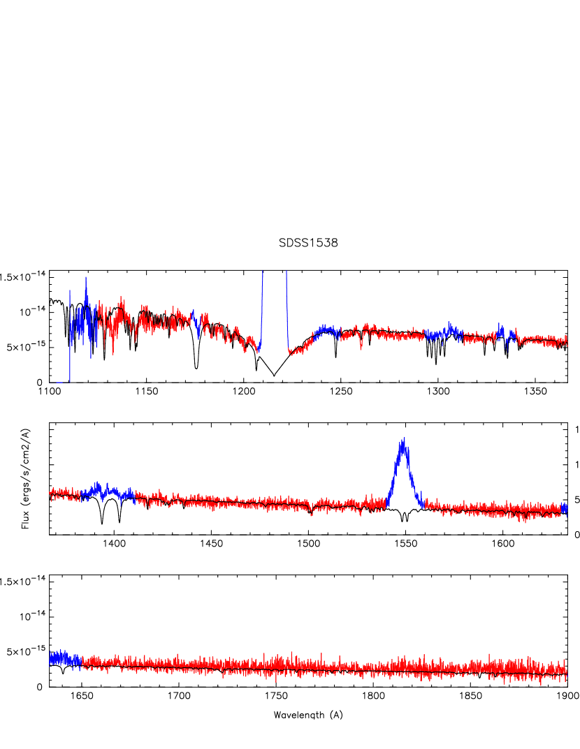
Figure 11: The spectrum of SDSS 1538 (in red) dereddened assuming E(B-V)=0.010 has been fitted with a WD model (in black). The model has a temperature of 35,875 K and gravity $log(g)=8.74$, with solar abundances and broadening velocity of 200 km/s. This COS spectrum is the co-added spectrum of the 4 COS subexposures. Regions in blue have been masked before the fitting and correspond to: the Ly$\alpha$ (1216) and O i ($\sim$1300) regions with air-glow emission; emission lines (or wings) from N iv ($\sim$1240), C ii (1335), Si iv ($\sim$1400), C iv ($\sim$1550); the C iii ($\sim$1175) line is very weak; and the lower edge of the detector. The Gaia distance to SDSS 1538 is $613^{+47}_{-41}$ pc.

5.1.2 Deriving Abundances and Rotational Velocities

In a second step, after we found the best $log(g)$ and $T_{\rm wd}$ fit for the spectrum, we vary the abundances of the elements Si, S, C, N, Fe, Al,.. one at a time, and vary the broadening velocity (assumed at first to be the projected WD stellar rotational velocity, $V_{\rm rot}sin(i)$) in the best fit model. The abundances are varied from $0.01\times$ solar (or lower if needed) to $50\times$ solar in steps of about a factor of two or so; the broadening velocity is varied from 50 km/s to 1000 km/ in steps of 50 km/s.

As in Godon & Sion (2021), Szkody et al. (2021) (see also Godon et al., 2017), the results of the abundances/velocity modeling are examined by visual inspection of the fitting of the absorption lines for each element. The reason we use visual examination rather than the $\chi^{2}$ minimization technique is that a visual examination can recognize and distinguish real absorption features from the noise, while the minimum $\chi^{2}$ is almost always obtained for the largest velocity model fitting the continuum but missing many absorption lines. This is because the spectral binning size of $\sim 0.58$ Å for STIS is of the same order of magnitude as the width of some of the absorption lines, and the depth of some of the absorption features is of the same amplitude as the flux errors. When the model is unable to reproduce some of the absorption lines, to compensate, the $\chi^{2}$ fitting drags the model continuum down (Long et al., 2006), and a lower $\chi^{2}$ is obtained for a higher broadening velocity. As a consequence, the best-fit in the $\chi^{2}$ sense doesn’t especially always provide the best-fit to the absorption lines, nor to the broadening velocity and can provide a larger distance (as the model continuum is dragged down).

Though the COS spectra have a higher resolution and S/N, we try (when possible) to fit the absorption lines in individual subexposures rather than in the co-added spectra (to avoid cumulative broadening due to the WD motion during the observation), and the subexposures are very often nearly under exposed.

The abundance analysis of SDSS 1538 is carried out by checking only the silicon and carbon lines, since, in any case, not many lines are present and Si and C lines dominate the spectrum. No ephemerides were found for SDSS 1538, however, the system is not eclipsing and all the 4 subexposures are similar. Consequently, we carry out the abundance analysis on the 4th subexposure to avoid line broadening due to the orbital motion of the WD during the observation. We found that carbon has to be very low, or the order of $\sim 0.0001$ solar, with a broadening velocity of 500 km/s, to model the absence of the C iii ($\sim$1175) line. Silicon appears to be solar (within a factor of about 2) with a velocity of $400\pm 100$ km/s, based on the absorption features in the shorter wavelengths, see Fig.12. The Si iv (1393.76,1402.77) doublet seems to be subsolar with a higher velocity ($>500$ km/s), however, this is due to some broad and shallow emission (which is better seen in Fig.2).

At first glance, it seems that the Si lines (at short wavelengths) in the model are too wide, but a lower broadening velocity produces sharper lines that do not especially match the shape of the observed features; a sign that some of these features might be due to noise. Deriving abundances from fitting the absence of absorption lines or weak absorption lines is more challenging (than fitting a spectrum with strong absorption lines) as the absorption features are of the same order as the noise.

Overall, the rest of the continuum does not disagree with solar abundance for the other species and a high velocity of 400 km/s, however, since the dominant absorption lines are from Si and C, this says little on the abundances of the other species.

From Fig.12, we see that the model does not reproduce the Si ii 1260 Å line, nor the C ii 1335 Å line. We tried to reproduce these lines with a very thin cold absorbing slab with a temperature $T=10,000$ K, an electron density $n_{e}=10^{13}$cm^-3, and a hydrogen column density $N_{\rm H}\approx 10^{18}-10^{19}$cm^-2. We find that the Si ii (1260) line always appears in the slab model together with the Si ii (1265) line, where the Si (1265) line is deeper than the Si (1260) line (just as in the WD photosphere model). Obviously, the Si (1260) line alone cannot form in the cold absorbing slab, nor in the WD photosphere. Similarly, to form in the WD photosphere, the C ii (1335) line requires such a carbon abundance that a strong C iii (1175) also forms. An extremely thin absorbing slab model with carbon solar abundance, a hydrogen column density of $\sim 10^{18}$cm^-2, and a turbulent dispersion velocity of $\sim 100$ km/s is, however, able to form such a a single C ii (1335) line alone with no other noticeable effect on the present spectrum. Since the Si (1260) and C (1335) lines both appear alone in the spectrum, it is also possible that they form in part in the interstellar medium (ISM, see e.g. Redfield & Linsky, 2004). In either case, this does not affect the results we obtain here for the WD abundances as we show that these lines do not form in the WD photosphere.

For the spectral analysis of the STIS and COS spectra of all the other systems, we follow exactly the same procedure as described here for SDSS 1538, except for the presence of an iron curtain and/or a second component when needed.

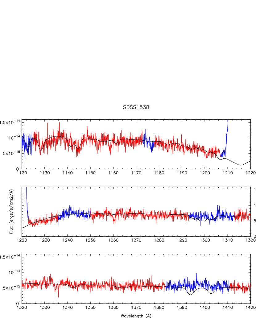
Figure 12: The 4th subexposure of the COS spectrum of SDSS 1538 dereddened assuming E(B-V)=0.010 has been fitted with a WD model. The model has a temperature of 35,875 K and gravity $log(g)=8.74$, with a carbon abundance of 0.0001$\times$ solar and silicon solar abundance. The broadening velocity is 400 km/s. What seems to be an absorption feature just below 1160 Å is a detector artifact. For convenience we only show the short wavelength range where all the absorption lines of interest are located. See text for details.

5.2 SDSS 1035: an Eclipsing WD without a Mask

The COS spectrum of SDSS 1035 is made of 8 subexposures with a rather low S/N. A look at the timing of the data (see Table 2, where the ephemerides of the system were taken from Littlefair et al. (2008)) indicates that only subexposures #7 and #8 cover the eclipse, which lasts approximately from $\Phi\approx-0.02$ to +0.02 (Savoury et al., 2011). Exposure #7 lasted from $\Phi\approx 0.01$ to $\Phi\approx 0.05$, while exposure #8 lasted from $\Phi\approx 0.82$ to $\Phi\approx 1.1$. The relative portion of the subexposures obtained during the eclipse is a very small fraction of the observing time, and both subexposures do not appear to have a flux that is noticeably lower than the other exposures. Because of the relatively low S/N of all the individual subexposures, we decided to combine all the subexposures together for the spectral analysis.

A preliminary modeling of the spectrum (with solar abundance WD models) shows that the WD has a temperature of the order of 11,000 K. At this temperature, silicon forms many strong absorption bands and carbon forms strong wide absorption lines. However, no such strong features are present in the COS spectrum of SDSS 1035. Because of that, the modeling of the spectrum with solar abundance WD models does not give reliable results for the temperature and gravity. Consequently, we lower the metallicity to a few percent (in solar units) to provide a best fit to the spectrum. We use the low abundance WD models to derive the WD temperature, gravity, abundances and broadening velocity.

For SDSS 1035, the final result, including all the errors, yields $T=11,475\pm 188$ K, with $log(g)=8.385\pm 0.166$. No second component and no iron curtain were necessary for the analysis.

Fitting the only clear line, C i ($\sim$1657), we obtain [Z]=0.03-0.05, with a broadening velocity $V=150\pm 50$ km/s. This best fit model is presented in Fig.13. We note that this model also fits the C i ($\sim$1561) absorption line.

SDSS 1035 is an eclipsing high inclination system, just like IR Com, but while the co-added COS spectrum of IR Com presents many WD absorption lines, the co-added COS spectrum of SDSS 1035 presents only one clear absorption line. Therefore, the absence of lines in SDSS 1035 is certainly not due to the broadening of the absorption lines from the WD orbital motion during the time of the observation (this is further discussed in Sec.6.2).

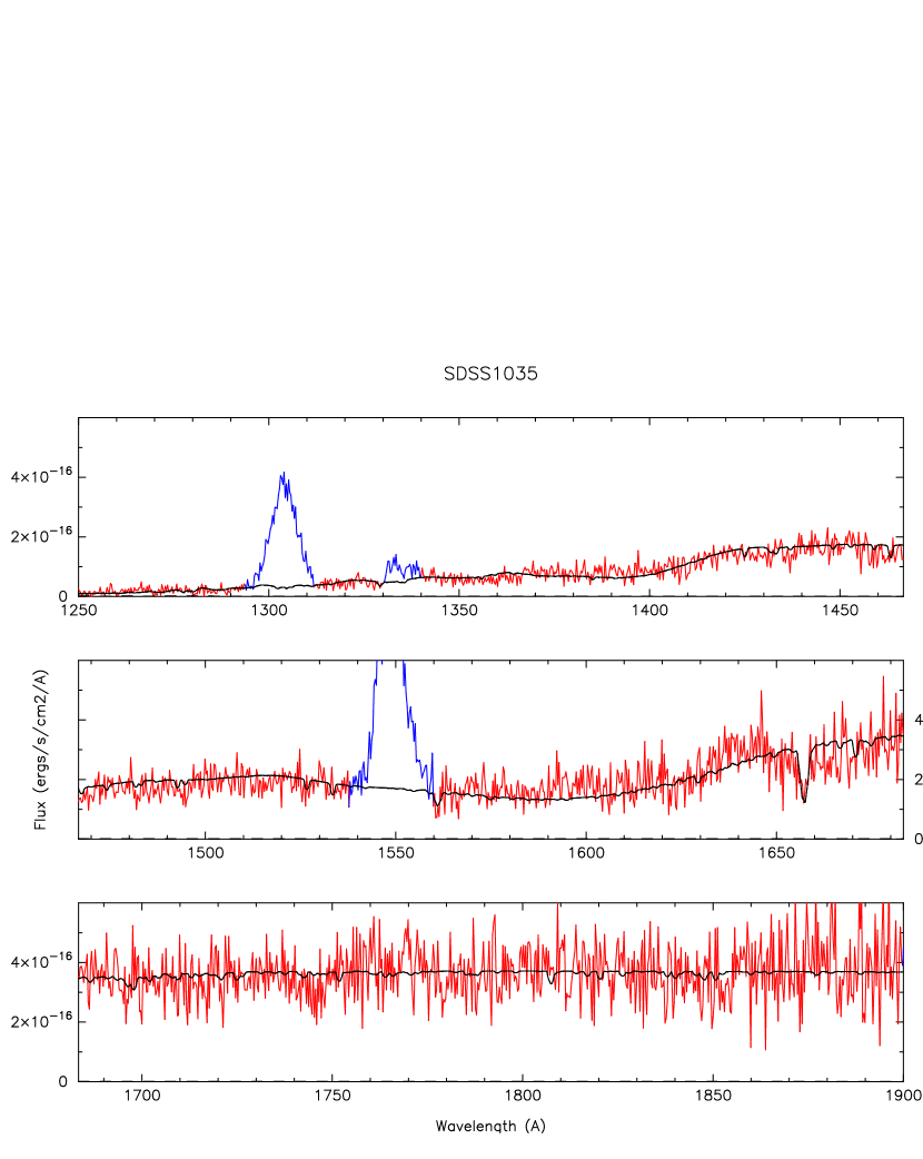
Figure 13: The spectral analysis of the COS spectrum of the WD in SDSS 1035 (in red) yields a solution (in black) with a temperature of $T=11,475\pm 188$ K, with $log(g)=8.385\pm 0.166$, metal abundance [Z]=0.03-0.05, and a broadening velocity $V=150\pm 50$ km/s. Strong emission lines have been masked before the fitting and are colored in blue. Below 1250 Å , the COS spectrum exhibits a continuum flux much smaller than the noise (see Fig.2) and only shows emission lines from C iii ($\sim$1175) and N v ($\sim$1240), as well as geocoronal emission O i ($\sim 1300$). The Gaia distance to SDSS 1035 is $195^{+12}_{-10}$ pc.

5.3 IY Ursae Majoris: Example of a Masked Eclipsing System

Since IY UMa is an eclipsing system showing strong absorption due to veiling material, we give here details of the iron curtain modeling and pay particular attention to the orbital phases at which each of the 4 subexposures of the COS spectrum were obtained.

The first subexposure exhibits a continuum flux level significantly lower than the other subexposures, an indication that it was obtained during eclipse. Subexposure #3 has the highest continuum flux level. The bottom of the Lyman$\alpha$ region undergoes the largest relative change: it has the lowest flux in exposure #1 and highest flux in exposure #3 (see Fig.14a). In addition, as expected for eclipsing systems, all exposures exhibit strong veiling, recognizable by the strong Fe ii absorption “bands” near $\sim 1565$ Å and $\sim 1635$ Å. We use the orbital period and ephemeris from McAllister et al. (2019, Table 1) to carefully and precisely time the subexposures as a function of the orbital phase. We find that exposure #3 (with the highest flux) was obtained at orbital phase $\Phi\sim$[-0.3,-0.1] (see Fig.14b), as the bright spot was facing the observer. During both exposures #1 and #4 the system went into eclipse, but exp.4 started before the eclipse and also had strong contribution from the bright spot. Exposure #2 is the only exposure obtained out of eclipse (at $\Phi\sim 0.2$) with little contribution from the bright spot. This exposure, like exp.1, has also very little flux at the bottom of the Ly$\alpha$ region, a possible indication that the bright spot is the reason the bottom of the Ly$\alpha$ does not go to zero in exp.3 & 4. We therefore decide to use subexposure #2 to carry out the spectral analysis of the WD in IY UMa. Unfortunately, this is also the shortest exposure with the lowest S/N.

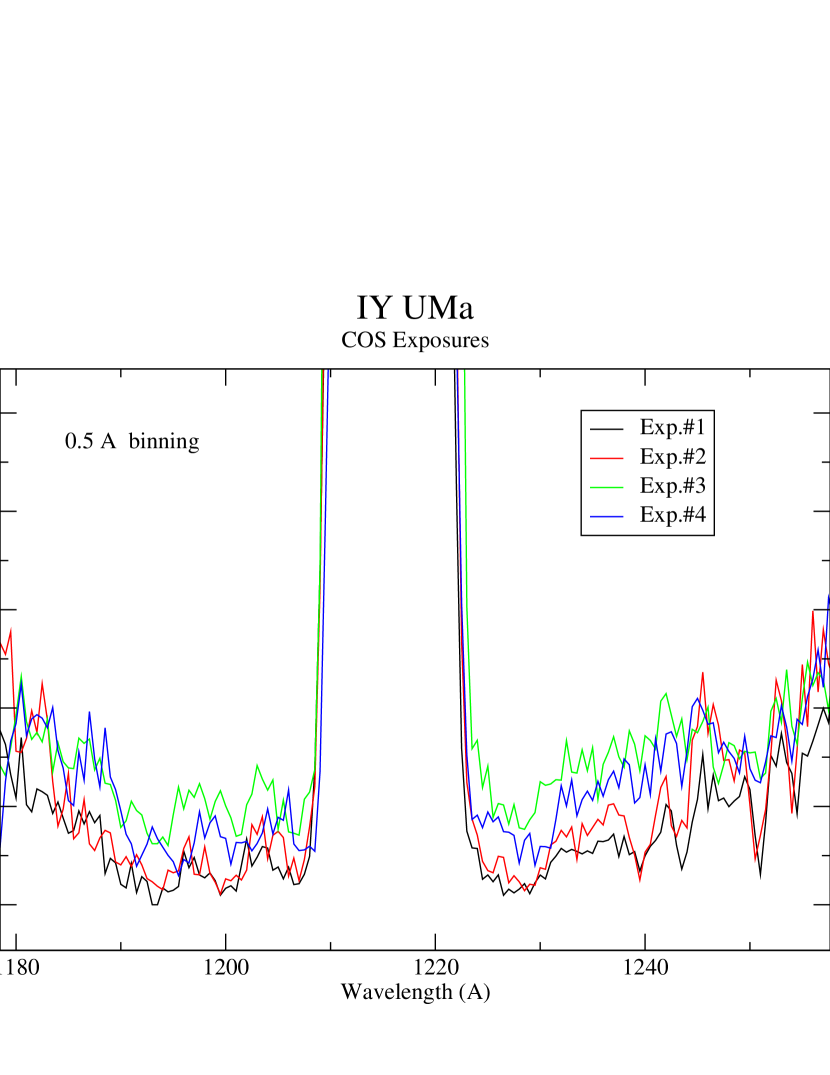
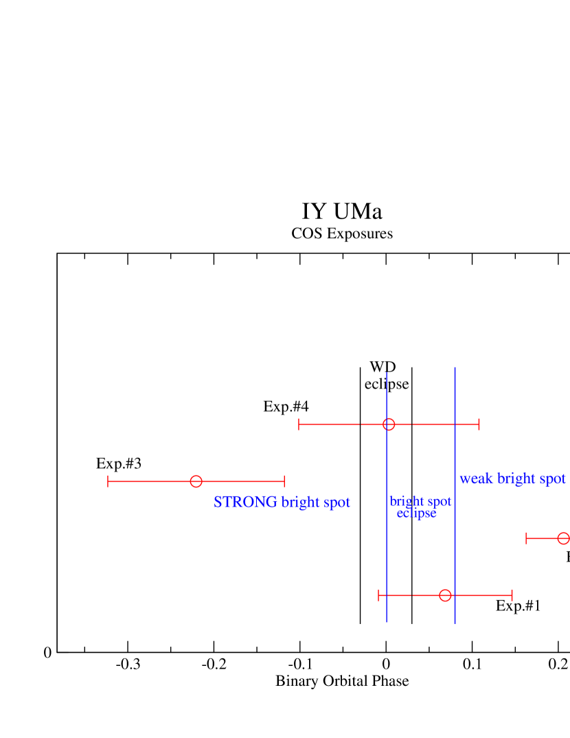
Figure 14: The 4 individual subexposures of the COS spectrum of IY UMa are presented. (a) Left. The individual subexposure spectra are shown in the Ly$\alpha$ region, where the most noticeable change is taking place. The flux level at the bottom of the Ly$\alpha$ is of the order of $1\times 10^{-15}$erg/s/cm²/Å in exposures # 3 & 4, and almost goes down to zero in exposures # 1 & 2. For convenience the exposures have been binned at 0.5 Å, and the vertical ($F_{\lambda}$) axis has been extended to $<0$. (b) Right. The subexposure duration and timing (in red) are shown as a function of the binary orbital phase (X-axis). The Y-axis is only used to present the subexposures in a staggered display. Exposures # 3 & 4 were obtained when the bright spot was facing the observer; during exposure # 1 & 4 the WD was eclipsed; only exposure # 2 was obtained when the WD was not eclipsed and with little contribution from the bright spot. The duration of each exposure is indicated by the length of the horizontal red mark. The WD eclipse is between the two vertical black lines and the bright spot eclipse is between the two vertical blue lines, as assessed from Fig.1 in McAllister et al. (2019).

The spectrum of IY UMa presents all the absorption features associated with the presence of veiling material. However, the spectral analysis of the second exposure of the COS spectrum of IY UMa was first carried out without an iron curtain, but with a second flat component with a flux of $2.5\times 10^{-16}$erg/s/cm²/Å (since even in subexposure #2 the bottom of the Ly$\alpha$ does not completely go down to zero). As explained explicitly in Sec.4.4, the continuum flux level of the second component was found by trial and error. For IY UMa, we increased the continuum flux level of the second component in steps of $5\times 10^{-17}$ and carried out the analysis, generating a $\chi^{2}$ map to find the best-fit for the given Gaia distance. We then chose the value of the second component that yielded the lowest $\chi^{2}$.

Following the same procedure as for SDSS 1538, we found the best fit for the single WD model, which occurs for the grid model with $T=17,000$ K and $log(g)=8.5$. Because the model still needs the addition of an iron curtain we did not fine tune the model to a higher accuracy at this stage. This model is presented in Fig.15a. That model has solar abundances and a projected WD stellar rotational velocity of 200 km/s. As expected, many absorption features are not fitted, especially in the longer wavelengths $\lambda>1550$ Å.

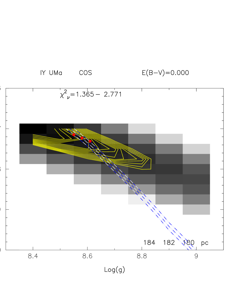
Figure 29: The $\chi^{2}$-map of the modeling of the second exposure of the COS spectrum of IY UMa is displayed. The modeling assumed a reddening of $E(B-V)=0.0$ and the WD model include an iron curtain and a second flat component. The solutions for the Gaia distance ($\pm$error) are shown with the 3 red dots.

In the next step, we added an iron curtain to the best fit WD model and varied the parameters of the iron curtain to fit the absorption features of the veiling material. For the iron curtain, we kept $T=10,000$ K and $n_{e}=10^{13}$cm^-3 constant, as suggested by Horne et al. (1994). The best fit is obtained for a hydrogen column density $N_{H}=10\pm 2\times 10^{21}$cm^-2, and a turbulent velocity $V_{\rm turb}=75_{-15}^{+25}$ km/s. Both the WD model and the iron curtain have solar abundances. We notice, however, that the addition of the iron curtain slightly changed to continuum flux level and the scaling to the Gaia distance of IY UMa. Therefore, we carried a new spectral analysis iteration. Namely, we generated veiled (with the above best fit iron curtain model) WD models in the $log(g)-T_{\rm wd}$ parameter space, and carried out a spectral analysis using these new veiled WD models (and with the above-mentioned second flat component). In other words, we obtained a $\chi^{2}$-map (Fig.29) in the $log(g)$ vs $T_{\rm wd}$ parameter space using a grid of veiled WD models: WD + absorbing slab, where the absorbing slab is the one given above.

The final results of the veiled WD model fits (including all the uncertainties) yielded $T=17,130\pm 249$ K, $log(g)=8.480\pm 0.125$, with solar abundances and a broadening velocity of 150 km/s. Such a model fit is presented in Fig.15b. The spectrum exhibits additional absorption from a much hotter medium with lines from C iii ($\sim$1175), Si iv ($\sim$1400), and C iv ($\sim$1550). The spectrum, when compared to the model, presents some broad emission near 1550 Å (C iv) as well as some higher flux in the shorter wavelength near 1250 Å, 1290 Å, and 1340 Å.

Many of the absorption lines in the COS spectrum of IY UMa are reasonably well fitted. We note the presence of the P ii (1452.89) absorption line in the model, which is not seen in the COS spectrum of IY UMa. In order to remove this line from the model we had to lower [P] to 0.01 solar, while keeping all the other elements to solar abundances (=1.0). The iron curtain fits pretty well (in depth and shape) the absorption lines from carbon, silicon, sulfur and iron. As no other P lines can be unambiguously modeled, one can question whether the abundance of phosphorus (based on a single line) is really subsolar or whether the iron curtain model needs further improvement. It is clear that the approach of a single iron curtain is only an approximation, since the iron curtain is made of a gas that is not isothermal, does not have constant density, nor a constant turbulent (dispersion) velocity. Ideally, one needs to construct an iron curtain with multiple layers, each with a different density, temperature, and velocity. Such a modeling is well beyond the scope of the present work.

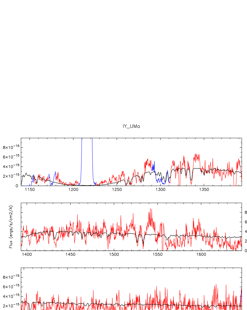
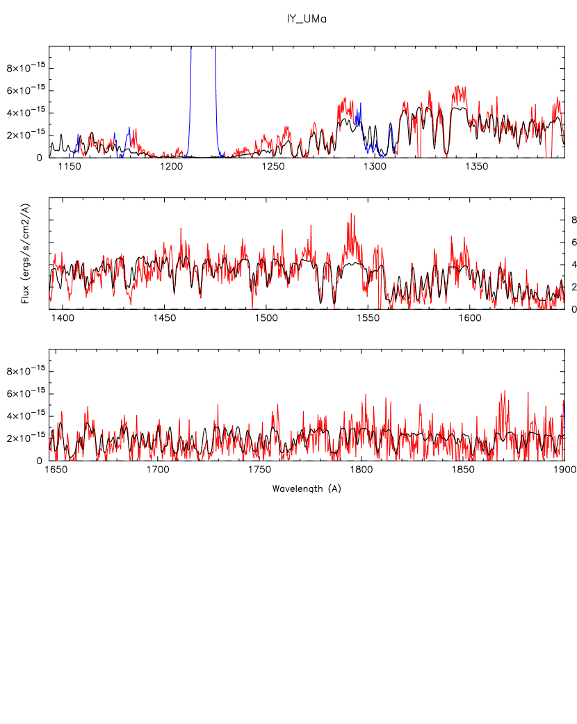
Figure 15: (a) Above. The second exposure of the COS spectrum of IY UMa is modelled with a WD synthetic spectrum. Many of the absorption lines are not fitted at all. Such a modeling gives a WD temperature of about 17,000 K, with a gravity $log(g)\approx 8.5$. The model has solar abundances and a broadening velocity of 200 km/s. (b) Below. The addition of an iron curtain greatly improves the fit. The iron curtain model has solar abundances, except for [P]=0.01. Its temperature is 10,000 K, with an electron density $n_{e}=10^{13}$cm^-3, turbulent velocity of $75^{+25}_{15}$ km/s, and an atomic hydrogen column density of $N_{\rm H}=10\pm 2\times 10^{21}$cm^-2. A second component with a constant flux of $2.5\times 10^{-16}$erg/s/cm²/Å has been taken into account in both cases. The Gaia distance to IY UMa is $182\pm 2$ pc.

5.4 DV Ursae Majoris

DV UMa is an eclipsing system with a STIS spectrum (a snapshot lasting only 900 s) obtained around orbital phase $\Phi\approx 0.2$. We carry out the analysis on this single exposure obtained out of eclipse. Because of its high inclination ($\sim 83^{\circ}$), the spectrum is heavily veiled. Consequently, we model a WD plus with the addition of an iron curtain in an iterative manner as done for IY UMa. Here too, the bottom of the Ly$\alpha$ does not go down to zero and, since this cannot be accounted for with the WD model (it is not hot enough with $T<20,000$ K), we take into account a flat second component with an amplitude of $1.16\times 10^{-16}$erg/s/cm²/Å (namely, we remove this constant flux from the observed spectrum). The first iteration of the WD plus iron curtain model fits yield a temperature of 19,500 K with $log(g)=8.6$ as shown in Fig. 16, where we present the WD model without (a) and with (b) the iron curtain.

The iron curtain, with a temperature of 10,000 K, electron density of $10^{13}$cm^-3, a turbulent velocity dispersion of 50 km/s, and a hydrogen column density of $3\times 10^{21}$cm^-2, significantly improves the fit in the longer wavelengths where the iron bands form ($\sim 1560$ Å and $\sim$1635 Å), but also in the shorter wavelengths near $\sim 1130$ Å and $\sim$1150 Å. However, some carbon lines appearing in the model spectrum do not show in the observed spectrum.

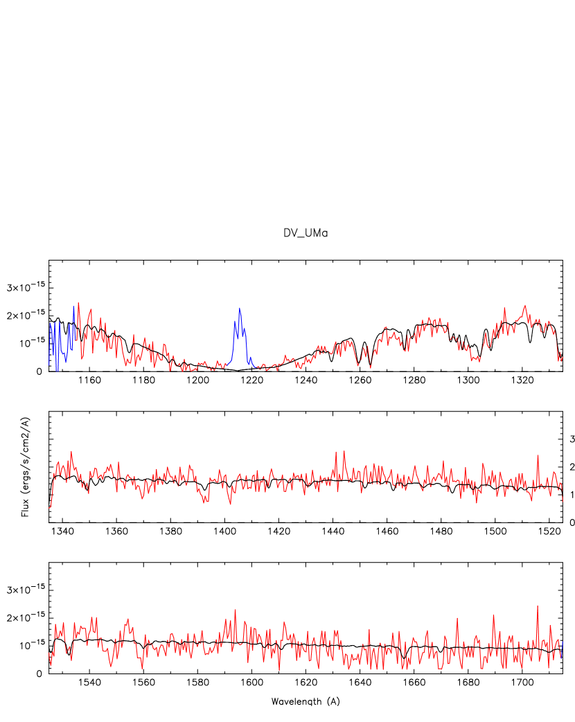
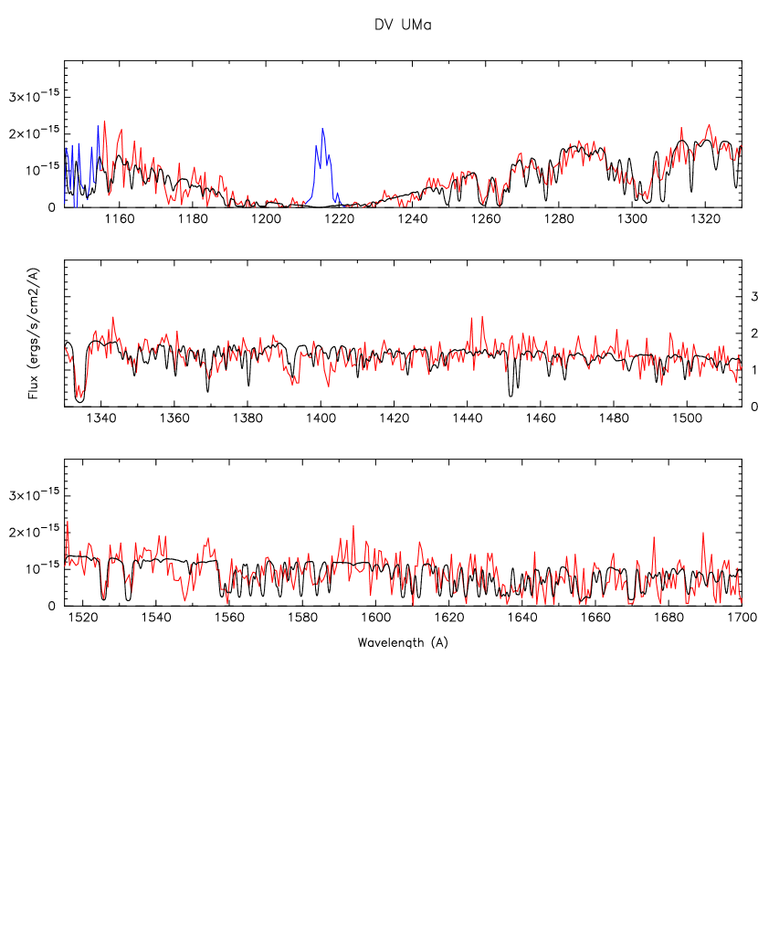
Figure 16: (a) Above. The STIS COS spectrum of DV UMa has been fitted with a WD model and taking into account a “flat” second component with a flux of $1.16\times 10^{-16}$erg/s/cm²/Å. The WD model has a temperature of 19,500 K, gravity $log(g)=8.6$, solar composition, and a broadening velocity of 150 km/s. (b) Below. An iron curtain has been added to the model to account for the many Fe ii absorption features. The iron curtain has a temperature of 10,000 K, electron density of $n_{e}=10^{13}$cm^-3, a velocity dispersion of 50 km/s, a hydrogen column density of $N_{\rm H}=3\times 10^{21}$cm^-2 and solar abundance. The Gaia distance to DV UMa is $387^{+24}_{-22}$ pc.

The iron curtain material is in all likelihood accretion material (e.g. overflowing the disk rim at the hot spot) and the WD surface composition is also made of the same accretion material (which is being replenished by accretion as diffusion takes place). Therefore, we assume that the WD photosphere and the iron curtain have the same composition, and we vary this composition to try and match as many absorption features as possible in the observed spectrum. We slightly vary the other parameters of the iron curtain in order to fine tune the fit.

We find that carbon, silicon and even phosphorus must be sub-solar, while the other elements are kept at solar values as they do not affect the fit. We find a carbon abundance [C]=0.1 solar (within a factor of two), silicon abundance [Si]=$0.3\pm 0.1$ solar, and phosphorus abundance [P]=0.01 solar or smaller. The low phosphorus abundance is needed since otherwise a strong P ii absorption line appears near 1452-3 Å, as seen in Fig.16b. This model is presented in Fig.17. The iron curtain in that model has a hydrogen column density of $2\times 10^{21}$cm^-2 and a turbulent velocity of 75 km/s. The final result of the fine tuning of the fit yields (with all the error bars included) $T_{\rm wd}=19,325\pm 481$ K, with $log(g)=8.565\pm 0.177$. Here too, it is difficult to fit all the lines, even of the same species. We note, a posteriori, that the left line of the sulfur doublet, near 1250-1255 Å, is not as strong in the STIS spectrum as in the model, an indication that sulfur is likely subsolar, i.e. [S]$<$1.0.

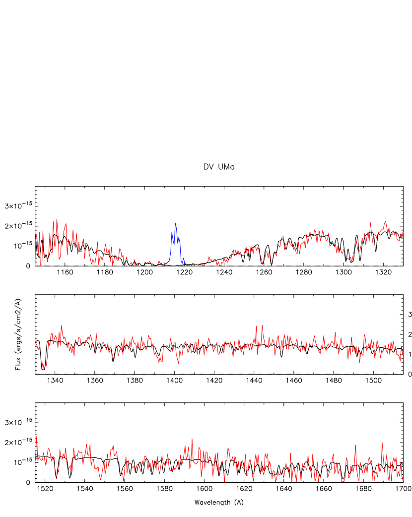
Figure 17: The final fit to the STIS spectrum of DV UMa yields a WD with a temperature $T_{\rm wd}=19,325\pm 481$ K, gravity $log(g)=8.565\pm 0.177$, and a broadening velocity $V=150$ km/s. The iron curtain has a temperature of 10,000 K, electron density of $n_{e}=10^{13}$cm^-3, a velocity dispersion of 75 km/s, a hydrogen column density of $N_{\rm H}=2\times 10^{21}$cm^-2. The iron curtain and the WD have the same abundances: [C]=0.1 solar, [Si]=0.3 solar, [P]$\lesssim$0.01 solar, with all the other elements having their solar value. A second component with a constant (flat) value of $1.16\times 10^{-16}$erg/s/cm²/Åwas also taken into account.

5.5 IR Comae Berenices

The COS data of IR Com is made of 5 subexposures. Subexposure #4 was obtained during eclipse (see Table 2) and has a significantly lower continuum flux level. The remaining 4 subexposures (#1, 2, 3, & 5) are very similar with the same continuum flux level; we combined them to generate a spectrum not affected by the eclipse, and we used that spectrum in our analysis. The bottom of the Ly$\alpha$ doesn’t go to zero, and we take a flat flux second component of $3.5\times 10^{-16}$erg/s/cm²/Å (at $E(B-V)=0.019$), which when subtracted from the spectrum brings the bottom of the Ly$\alpha$ to zero. The spectrum of IR Com does not exhibit any iron absorption bands characteristic of the iron curtain, in spite of the fact that this is a high inclination eclipsing system (which was also the case for SDSS 1035). Consequently, we carried out the analysis without iron curtain modeling. The results of the single WD analysis yield a WD temperature $T_{\rm wd}=17,860\pm 180$ K, and gravity $log(g)=8.613\pm 0.090$. The fitting of the absorption lines yields solar abundances, except for aluminum with [Al]=$5\pm 1$ solar, based on Al ii (1670.8) and Al iii (1854.7 & 1862.8) lines, and iron [Fe]$\sim 4\pm 1$ solar, which slightly improves the fit in the very short wavelength and very long wavelength regions. We found a broadening velocity of $150\pm 50$ km/s (see Fig.18a). Except for the very short wavelength region ($\lambda<1160$ Å), the COS spectrum is relatively well fitted with the WD model spectrum.

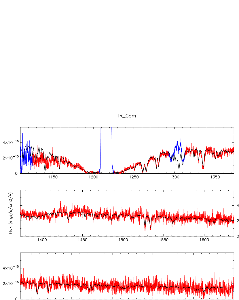
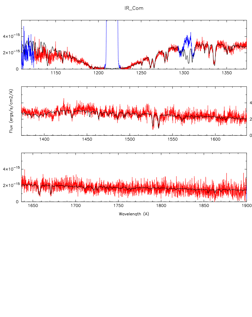
Figure 18: (a) Above. The analysis of the COS spectrum of IR Com yields a WD temperature of $17,860\pm 180$ K, gravity $log(g)=8.613\pm 0.090$, and elevated abundance of aluminum ([Al]$=5\pm 1$ solar) and iron ([Fe]=$4\pm 1$ solar) with a broadening velocity $V=150$ km/s. (b) Below. The addition of a thin iron curtain increases the depth of aluminum and iron lines without the need to have suprasolar aluminum and iron abundances in the WD model. The Gaia distance to IR Com is $217\pm 3$ pc.

We note that in DV UMa and the other veiled systems (e.g. GY Cnc and BD Pav), the short wavelength region $\lambda<1160$ Å  is also affected by Fe ii absorption lines, creating two adjacent absorption bands at $\sim 1130$ Å and $\sim 1150$ Å in addition to the Fe absorption bands seen near $\sim 1565$ and $1635$ Å, raising the possibility that the COS spectrum of IR Com might also be affected by an iron curtain. Consequently, we added a cold absorbing slab/iron curtain model ($T=10,000$ K, $n_{e}=10^{13}$cm^-3, and solar abundances) to the stellar WD model, to check whether the short wavelength region fit could be improved.

We obtained a better fit in the short wavelength region for an absorbing slab with a hydrogen column density of $N_{\rm H}=5\times 10^{20}$cm^-2 and a turbulent velocity of $\sim$100 km/s. However, such an iron curtain also creates strong absorption bands at 1565 and 1635 Å and strong C and Si lines which are not observed. Since the absorption bands at 1565 & 1635 Å  and the absorption feature at $\lambda<1160$ Å are all due to iron, one cannot generate one without generating the other (even by changing the temperature and density of the iron curtain). Such an iron curtain had to be ruled out.

However, we found that an thin absorbing slab with a hydrogen column density of only $N_{\rm H}=1\times 10^{19}$cm^-2 and a turbulent velocity of 100 km/s slightly improves the WD fit in the shorter wavelengths, and also helps fit the aluminum and iron lines without the need to increase [Al] and [Fe] abundances above solar in the WD model. This thin iron curtain model exhibits a slightly deeper C ii (1335) absorption line, and we therefore had to decrease the carbon abundance in the curtain to [C]=0.4 while keeping solar abundance for the WD model (in order to match the carbon 1330 line).

We present this solar abundance WD with a thin iron curtain model in Fig.18b. There is little difference between the WD model (Fig.18a) and the WD plus iron curtain model (Fig.18b). Because of this, it is not clear whether the WD has increased iron and aluminum abundances or just a thin iron curtain. The fact that the shorter wavelength region is not adequately modeled may imply that our model might be inaccurate or incomplete, or might point out to some calibration problems at the inner edge of the detector. Overall, the results indicate that the WD does have nearly solar abundances. We further discuss the thin iron curtain of IR Com in Sec.6.4.

5.6 GY Cancri

The STIS snapshot spectrum of the eclipsing system GY Cnc was obtained around binary orbital phase $\Phi\approx 0.25$, well out of eclipse ($i\sim 77^{\circ}$), in spite of that, it reveals a heavily veiled WD similar to the spectra of IY UMa and DV UMa (with $i>80^{\circ}$).

We modeled the spectrum of GY Cnc with a WD plus an iron curtain in the same iterative manner as we did for IY UMa and DV UMa, using first solar abundances. We also took into account a second flat component of amplitude $2\times 10^{-15}$erg/s/cm²/Å. The best fit yielded a gravity $log(g)=7.876\pm 0.108$ with a temperature $T_{\rm wd}=22,515\pm 292$ K, and a WD projected stellar rotational (broadening) velocity of 150 km/s, for a distance of $275\pm 5$ pc, reddening $E(B-V)=0.023\pm 0.013$, including the propagation of the uncertainties from the statistical error, the modeling, and the instrumental/detector errors (as was done for all other systems). The iron curtain model has a relatively large atomic hydrogen column density, $5\pm 1\times 10^{21}$cm^-2, with a turbulent velocity of $75\pm 25$ km/s. This model is presented in Fig.19 with and without an iron curtain.

The iron curtain does model relatively well the many iron absorption features in the longer wavelengths $\sim 1500-1700$ Å, since these are the absorption features that we use in the fit to derive the iron curtain parameters. The strong emission lines of H i (1216), Si iv ($\sim$1400), C iv ($\sim$1550) are not fitted and are strongly blue-shifted, indicating they form in a wind. Strong absorption lines (not shifted) are present on top of the Si iv and C iv emissions, as well as N v ($\sim$1240) absorption lines; they too form in a hotter gas and are not modeled here. While we do not attempt to fit these features forming in a hot gas, some low ionization sulfur ($\sim 1250$), silicon ($\sim 1260$), carbon ($\sim 1330$), and phosphorus ($\sim 1452$) absorption lines are too deep in the model.

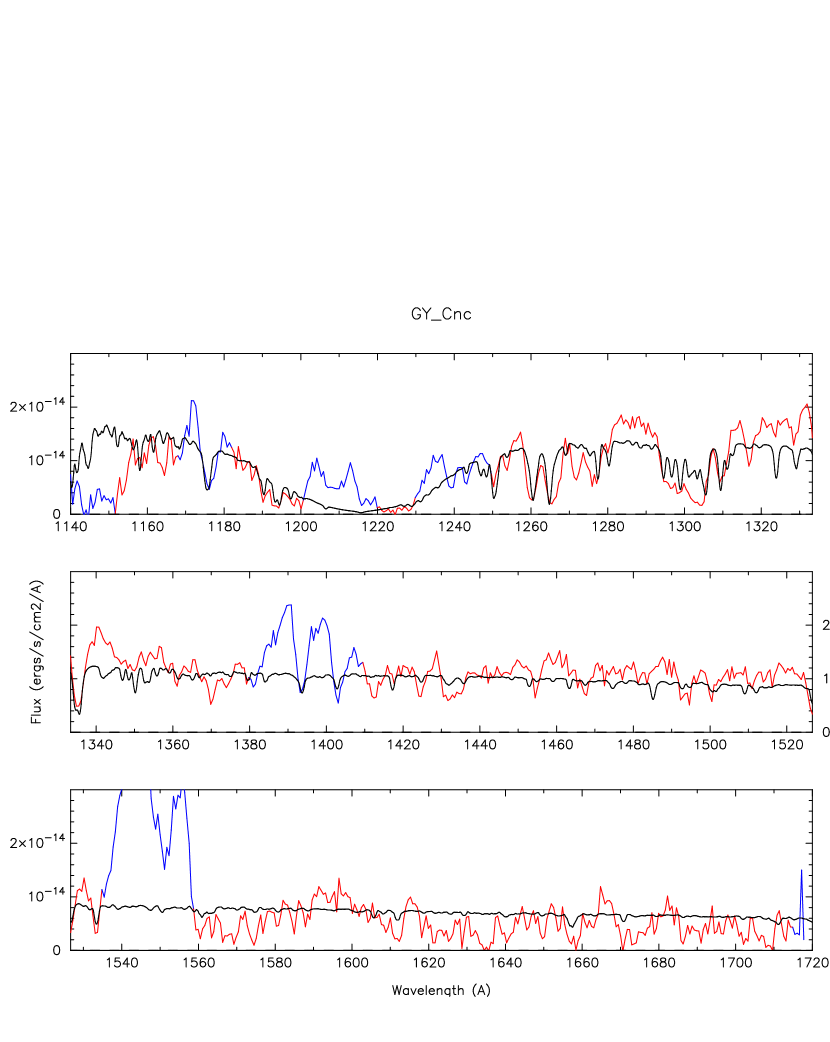
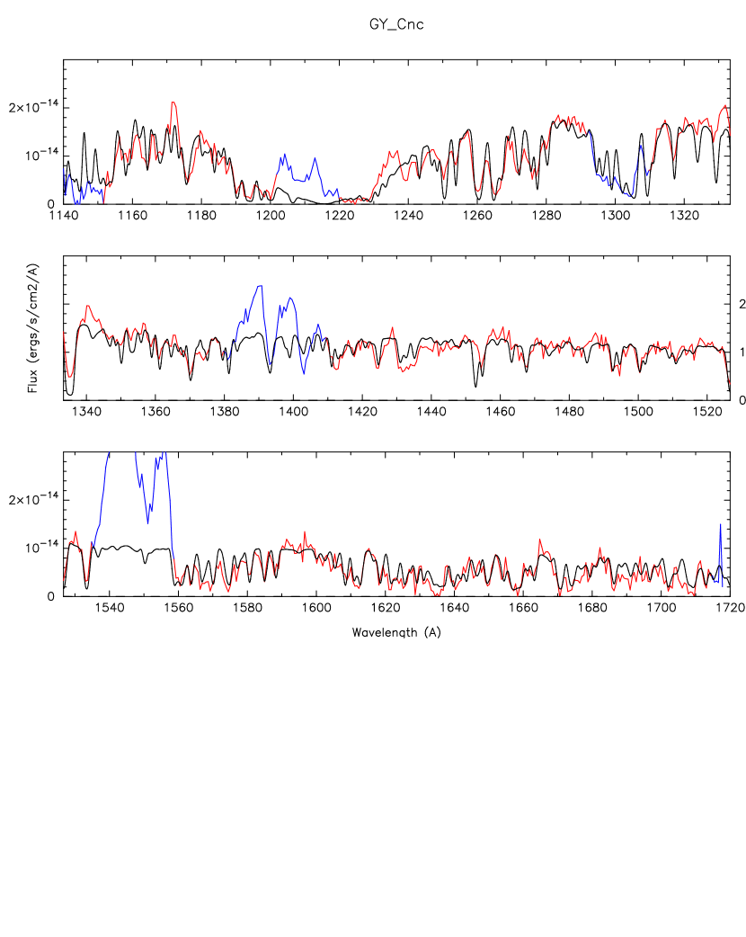
Figure 19: The final results of the modeling of the spectrum of GY Cnc is a WD with a temperature $T_{\rm wd}=22,515\pm 292$ K, gravity $log(g)=7.876\pm 0.108$, and a broadening velocity of 150 km/s. (a) Above. A single WD model alone is inadequate to fit most of the spectral features especially in the longer wavelengths. (b) Below. The addition of an iron curtain significantly improves the fit. Both the WD stellar model spectrum and the iron curtain have solar abundances. The Gaia distance to GY Cnc is $275^{+5}_{-4}$ pc.

In order to improve the fit, we lower the abundances of C, Si, P, and S in both the WD and the iron curtain to better fit these lines. We find the best fit for [C]=0.01, [P]$\lesssim$0.01, [Si]=[S]=0.1, presented in the Fig.20. However, while the above mention line fit improved, the fit to some of the other lines (in the $\sim 1160$ Å and $\sim 1300$ Å regions) is slightly degraded. From this new fit, it seems more apparent that C iii ($\sim$1175) and N v ($\sim$1240) have some broad emission. C ii (1335) also presents some emission. Overall the non-solar abundance model improves the fit and points to subsolar abundances.

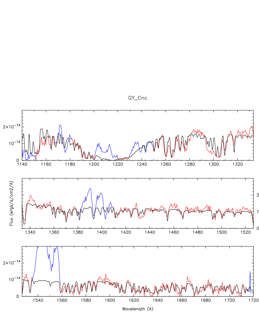
Figure 20: The same WD and iron curtain model as in Fig.19 is presented here, but now both the WD and iron curtain have non-solar abundances: [C]=0.01, [Si]=0.1, [P]=0.01, and [S]=0.1. See text for details.

5.7 BD Pavonis

The COS data of BD Pav consists of 5 subexposures. Subxposure #1 was collected from orbital phase $\Phi=0.87$ to $\Phi=1.00$ with a continuum flux level about 20% lower than subexposures #2 and #3 (obtained at orbital phases $\Phi=0.26$ and 0.36, respectively), but only 5 to 10% lower than subexposures #4 and #5 (obtained at $\Phi=0.61$ and 0.70). With an inclination not higher than $75^{\circ}$, BD Pav shows signs that its WD is eclipsed (Kimura et al., 2018, barely eclipsed), explaining the lower flux in subexposure #1. Exposures #2 and #3 have a higher flux as well as stronger emission lines, pointing to the possibility of a (relatively) hot emitting component (which could be the second component which we model with a flat continuum). It is not clear neither, whether subexposures #4 and #5 have a lower flux (than subexposures #2 and #3) due to stream-disk overflow material (as is often the case around $\Phi=0.6-0.8$), or have an unaffected continuum flux level. All the subexposures show signs of strong veiling, and all exhibit the same absorption lines. Since one cannot clearly identify which of the subexposures had a “clear shot” at the WD, we decided to combined the 5 exposures and carry out the analysis on the combined spectrum. We estimate that the continuum flux level of the combined spectrum cannot be more than 10% off from the unaffected spectrum of the WD itself. Since we perform the analysis taking into account a second component, it is more likely that the combined spectrum continuum flux level is only a few % off. For that reason, we included an additional error of 10% in the continuum flux level to the final results, (for comparison such an error corresponds to an error of $\sim 3.16$% in the distance).

The final result of fitting a WD model to the COS spectrum of BD Pav yielded a temperature of $19,330\pm 312$ K, gravity $log(g)=8.117\pm 0.158$, for a distance of $333\pm 3$ pc, reddening $E(B-V)=0.057\pm 0.018$. Two WD fits are presented in Fig.21.

In Fig.21a we present one of the solar abundance grid models with $T=19,500$ K, $log(g)=8.1$, without an iron curtain, nor a second component. Overall, the model fits the continuum flux level and some of the absorption lines, but it fails to fit the very short wavelengths ($\lambda<1160$ Å) as well as many absorption features seen in the longer wavelengths ($\sim 1500$ Å). This is a sign that an iron curtain is needed to better fit the spectrum.

We also carried out a (iterative) WD plus iron curtain fit as we did for IY UMa and also included a second component of amplitude $7\times 10^{-16}$erg/s/cm²/Å. We first assumed solar abundances for the WD and iron curtain, but such a model also produced much more pronounced Si ii and C i+C ii absorption lines that do not agree at all with the data. We noticed also that even the single WD model produced carbon absorption lines (e.g. at 1140, 1160, 1325, and 1330 Å) that are not observed. We therefore decided to vary the abundances of carbon and silicon in both the iron curtain and the WD model. As mentioned before, since the metals observed in the photosphere of the WD are due to accretion, we set the WD and curtain abundances to the same values in the model. We found that we have to lower the carbon and silicon abundances to fit most of the carbon and silicon lines. The WD with the iron curtain model still produced two strong lines that do not fit: one aluminum line (Al i 1371.01 Å) and one phosphorus line (P ii 1452.89 Å), both too strong in the model. Consequently, we also lower Al and P abundances to fit the data.

The final result is presented in Fig.21b. The abundances we obtained are [C]=$0.01_{-0.005}^{+0.01}$, [Al]=0.1${}_{-0.05}^{+0.1}$, [Si]=0.1${}_{-0.05}^{+0.1}$, and [P]$\lesssim 0.01$ (assuming [Z]=1 for all other species including Fe) in solar units for both the WD and its curtain. The broadening velocity is $200\pm 50$ km/s. Here too, we notice that the sulfur doublet is slightly deeper in the model than in the observed spectrum, indicating that sulfur is likely subsolar: $[S]<1.0$ solar. As with all other systems, the cold iron curtain has a temperature of 10,000 K with an electron density of $n_{\rm e}=10^{13}$cm^-3 (Horne et al., 1994). The turbulent velocity dispersion for the modeling of BD Pav iron curtain is $200\pm 50$ km/s, together with a hydrogen column density of $N_{\rm H}=1.0_{-0.5}^{+}{1.0}\times 10^{21}$, which are needed to produce the strong iron absorption features.

In the final model, the absorption that are not fitted are due to higher ionization, i.e. C iii ($\sim$1175), N v ($\sim$1240), Si iv ($\sim$1400), and C iv ($\sim$1550), all forming in a much hotter gas. We do not model this hotter gas, nor do we model the emission lines. The spectrum also presents some broad emission lines of N v ($\sim$1240), Si iv ($\sim$1400), and He ii ($\sim 1640$) that we do not attempt to model. We also ignore the Ly$\alpha$ and $\sim 1300$ Å regions as they are contaminated with daylight/airglow.

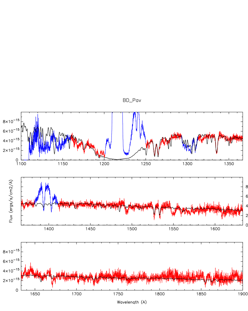
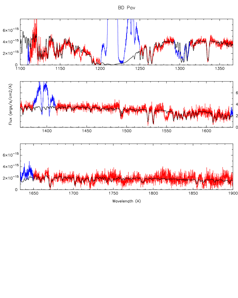
Figure 21: Above.(a) The spectrum of BD Pav (in red) has been fitted with a WD model (in black), with a temperature of 19,500 K, gravity $log(g)=8.1$, with solar abundances and broadening velocity of 200 km/s. The region below 1160 Å could not be fitted and was masked together with the regions contaminated by airglow and strong emission lines (in blue). Below. (b) The addition of an “iron curtain” to the WD model greatly improves the fit, especially in the shorter wavelengths region. Both the iron curtain and WD models have subsolar carbon and silicon abundances. A second component was taken into account. The Gaia distance to BD Pav is $333\pm 3$ pc.

5.8 HS 2214+2845

The COS data of HS 2214 consists of 4 subexposures obtained on 4 slightly different positions on the detector, slightly shifted relative to each other. The continuum flux level is the same in all the exposures, well within the error bars, and the only difference is in the absorption lines. Therefore, we decided to start the analysis on the combined (co-added) spectrum to derive the WD surface temperature and gravity, and to use the subexposures to derive the WD surface abundances and broadening velocity.

The spectrum does not exhibit any sign of veiling and we carried out WD model fits without an iron curtain. We found that the addition of a small second component (of amplitude $1.5\times 10^{-15}$erg/s/cm²/Å) slightly improves the fit. The WD temperature is $T_{\rm wd}=27,643\pm 268$ K, with a gravity $log(g)=8.30\pm 0.16$, for a distance of $400\pm 8$ pc, and reddening $E(B-V)=0.052\pm 0.023$. Such a model fit is presented in Fig.22, with solar composition and broadening velocity $V=250$ km/s. The model fits only a few absorption lines and presents more lines than the observed spectrum. We then turned to the individual subexposures to model the absorption lines.

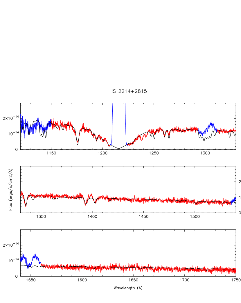
Figure 22: The COS spectrum of HS 2214+2845 (in red) has been fitted with a synthetic WD model spectrum (in black) to derive the WD temperature and gravity, for a distance of $400\pm 8$ pc. The best fit yields a solution $T_{\rm wd}=27,643\pm 268$ K, $log(g)=8.30\pm 0.16$. This models assumes a velocity broadening of 250 km/s and solar composition. The regions in blue have been masked before the fitting. The fitting of the absorption lines is done separately in a different fit using individual subexposures. The Gaia distance to HS 2214+2815 is $400\pm 8$ pc.

From the timing of the subexposures (see Table 2), the first subexposure was obtained at orbital phase $\Phi=0.312$ (the WD was moving toward the observer), subexposure #2 at $\Phi=0.522$ (the WD was facing the observer), subexposure #3 at $\Phi=0.635$ (the WD started receding from the observer), and subexposure #4 at $\Phi=0.041$ (when the secondary was facing the observer). The shift observed in the absorption lines is consistent with and confirms the above timing of the subexposures, with one exception: in subexposure #1 the C iii ($\sim$1175) absorption line is blue shifted by 3 Å. Though, this could be due to hot material ejected toward the observer around $\Phi\sim 0.3$, it is also the very edge of the COS detector in the COS position in which this exposure was set. We, therefore, ignore this 3 Å blueshift.

To derive the chemical abundances of the WD surface, we choose to fit subexposure #2, since at the time the data was collected the WD was facing the observer. In addition, an important feature in the second exposure is the complete absence of the N v doublet ($\sim$1240) absorption lines, which are observed in the other three exposures. Also, the absorption lines of C iii ($\sim$1175), C ii (1334), Si iv ($\sim$1400), and C iv ($\sim$1550) are not as pronounced in subexposure #2 as in the other exposures. The N,v (1240), and C iv ($\sim$1550) absorption lines form in a much hotter gas and are not associated with the WD photosphere, and to some extent the C iii ($\sim$1175) and Si iv ($\sim$1400) lines, though they form in the WD photosphere at this temperature and gravity, might too be forming, in part, in the same hotter gas. Altogether, subexposure #2 is less affected by these higher ionization species absorption lines and is more representative of the WD spectrum. The continuum flux level in subexposure #2 is otherwise the same as in the other subexposures.

The fit to subexposure #2 (Fig.23a) gave a subsolar silicon abundance [Si]=$0.2\pm 0.1\times$solar, with a broadening velocity $V=400\pm 50$ km/s. All the other metals were kept to solar abundances [Z]=1. The low silicon abundance together with the high broadening velocity were needed to fit the shallow absorption line near 1194 Å, 1260 Å and 1265 Å. Even the 1300 Å region, which can potentially be affected by airglow (as in exposure 4), is, too, well fitted.

For comparison, in Fig.23b, we show exactly the same model fit together with subexposure #4. One can clearly distinguish deeper absorption lines of C iii ($\sim$1175), C ii (1335), Si iv ($\sim$1400) and C iv ($\sim$1550), as well as the appearance of new absorption lines of N v ($\sim$1240) and Si ii (1260 & 1265).

The shift in the higher ionization species absorption lines follows roughly that of the WD, indicating that they form near the WD, in (or more likely above) the hot inner disk. The reason these lines are attenuated or disappear near phase 0.5 (exposure #2) is possibly be due to L1-stream cold material overflowing the edge of the disk and landing near phase 0.5-0.6 (see e.g. Lubow, 1989; Godon, 2019) on the disk face near the WD. This material might reduce the scale height of the ionized material above the inner disk face, pushing it down toward the disk mid-plane and out of the line of sight of the observer toward the WD, thereby removing from the spectrum the absorption lines forming in the hot ionized material. Such a scenario requires a moderate inclination. The 4 exposures have the same continuum flux level, indicating that there is not eclipse, occultation, or any other strong veiling of the WD.

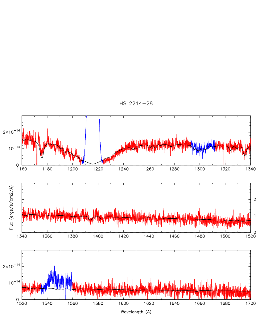
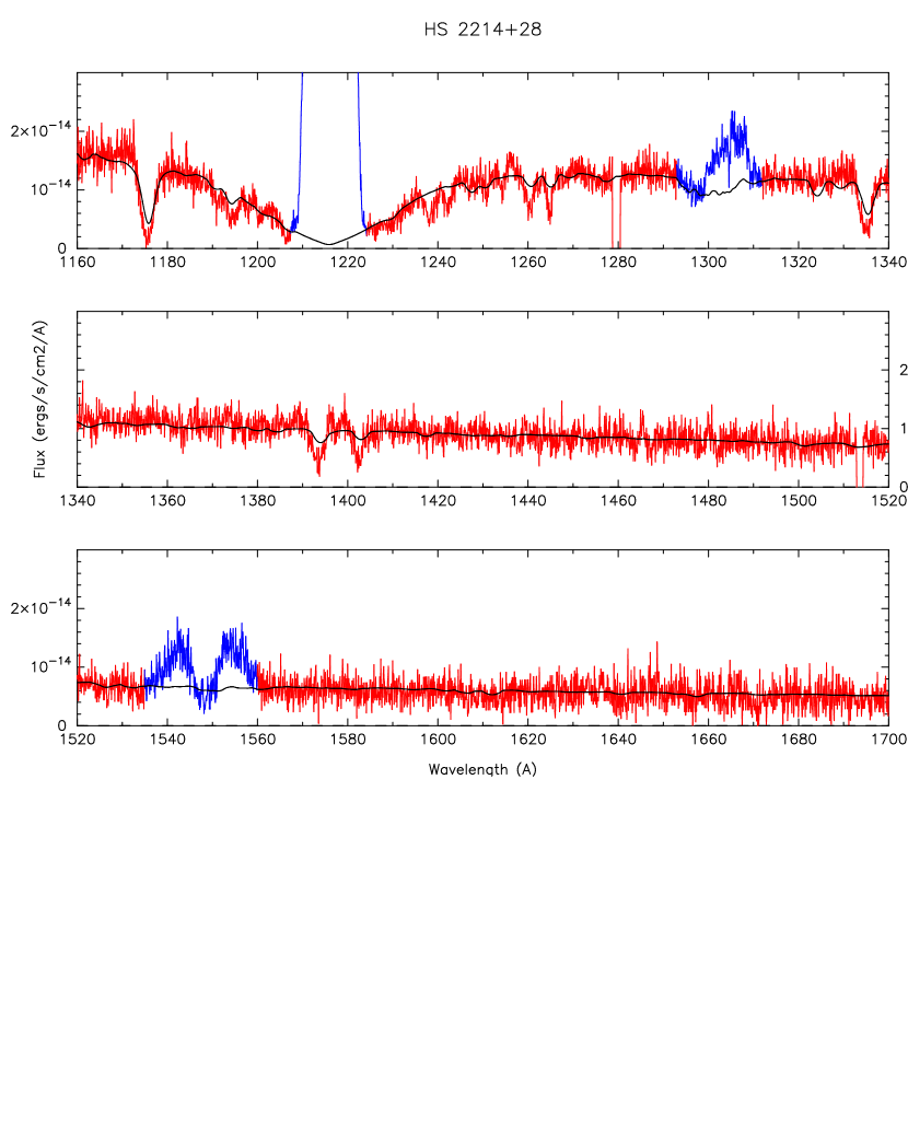
Figure 23: (a) Above. The subexposure #2 (in red) of the COS spectrum of HS 2214+2845, obtained at orbital phase $\sim 0.5$ (WD facing the observer), is used to derive the WD surface abundances and broadening velocity. The model (in black) is the same as presented in Fig.22, except for a silicon abundance [Si]=0.2 solar (while keeping the other species to solar) and a broadening velocity of 400 km/s. (b) Below. For comparison, subexposure #4, obtained near orbital phase 0.0 (secondary facing the observer) shows stronger absorption lines, as well as the apparition of additional lines, not seen in subexposure #2, but present in all other subexposures. The [Si]=0.2 model is also shown for comparison.

5.9 TT Crateris

The STIS snapshot spectrum of TT Crt was obtained near binary orbital phase $\Phi=0.29$, and with an inclination of $\approx 50-70^{\circ}$, it is not eclipsing nor is it expected to suffer from veiling. We therefore carried out a single WD fit to the STIS spectrum, first assuming solar composition. We found the need to add a second flat component of amplitude $5\times 10^{-16}$ erg/s/cm²/Å. The analysis yielded a temperature of $26,990\pm 557$ K with a gravity $log(g)=8.044\pm 0.097$, for a distance $d=547_{-12}^{+14}$ pc and reddening $E(B-V)=0.020\pm 0.009$, including the propagation of all the errors. This model is presented in Fig.24, from which it is apparent that the absorption lines do not agree with solar abundances. The best matches, though far from being perfect, are for the C iii ($\sim$1175) line (which would be better fitted with a lower C abundance) and with the C ii (1335) line (which would be better fitted with a higher C abundance and higher velocity). All the silicon lines would be better fitted with both a higher velocity and a higher Si abundance.

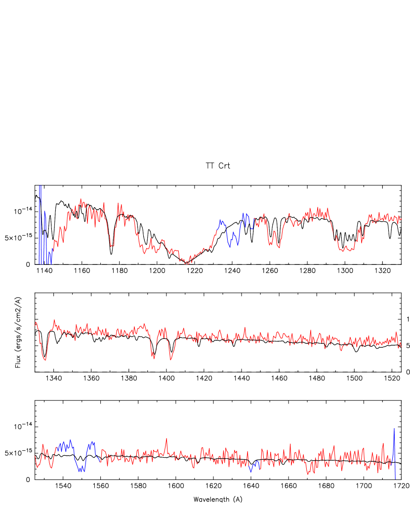
Figure 24: The results of the spectral fit of the STIS spectrum of TT Crt indicate a WD temperature $T_{\rm wd}=26,990\pm 557$ K with a gravity $log(g)=8.044\pm 0.097$. This model has solar abundances with a 200 km/s broadening velocity. The Gaia distance to TT Crt is $547^{+14}_{-12}$ pc.

Consequently, next, we varied the chemical abundances of the WD model as well as the broadening velocity in order to match the absorption lines. We found that a higher velocity together with higher abundances help fit the C ii (1335) & C iii ($\sim$1175) lines as well as the $\sim 1300$ Å Si ii+iii feature. A best fit was obtained for [Z]=5 (in solar units) with a broadening velocity of 400 km/s. This model is presented in Fig.25a. However, many of the other C and Si absorption lines are not well fitted. The Si ii (1194, 1260, 1265), Si iv ($\sim$1400) lines require a higher Si abundance, while the absence of Si iii (1343, 1360) lines require a lower Si abundance. Similarly, the absence of C i (1325, 1330) lines also require a much lower C abundance. A possibility is that many of the lines that are observed do not form in the stellar photosphere. Of course the C iv ($\sim$1550) line with its emission wings form in a much hotter gas, which could also partially contribute to the C iii ($\sim$1175) and Si iv ($\sim$1400) lines.

The absence of C i (1325, 1330) lines in GY Cnc was due to the fact that most lines formed in the iron curtain. In addition, we note that the spectrum of TT Crt shows absorption lines near 1610 Å, 1670 Å, and 1700 Å, which are prominent in the strongly veiled spectrum of DV UMa and BD Pav, and are due to the iron curtain. Hence, in the next step, we included an iron curtain in the modeling. We assumed solar iron abundance for the curtain and varied its parameters (i.e. turbulent velocity and hydrogen column density) to match the spectrum of TT Crt in the longer wavelengths. A best fit gave a turbulent velocity of $100\pm 25$ km/s with a hydrogen column density if $5\pm 2\times 10^{20}$cm^-2. Keeping these two parameters constant, we then varied the silicon abundance of both the iron curtain and WD (assuming again that they are equal) to match the Si ii (1526.7 & 1533.4) doublet (which does not from in the WD stellar photosphere at this gravity and temperature). We found that we have to lower it to [Si]=0.1. We then try and fit the C ii (1335) feature, and find [C]=0.01. We lower [S] to 0.1 since the S i+ii ($\sim 1250$) lines are also very weak. And again we set [P]=0.01 as the P ii (1452.89) is not observed. The need to lower all these abundances is because many lines in the iron curtain are very strong, even when assuming solar abundances. The low abundances of C, Si, P and S produce shallow absorption lines in the WD stellar spectrum itself which are almost negligible when compared to the absorption lines due to the iron curtain. This model is presented in Fig.25(b). Here too, the fit is consistent with a hot gas (not modeled) contributing to the absorption lines of C iii ($\sim$1175), Si iv ($\sim$1400), and C iv ($\sim$1550). We also note that, while the iron curtain provides a reasonable fit to the 1610 Å,1670 Å, and 1700 Å absorption features, it also fits the region 1560-1590 Å pretty accurately, which could easily be confused with noise. The small 1640 Å absorption feature is due to He ii and does not form in the (cold) iron curtain nor in the WD stellar photosphere.

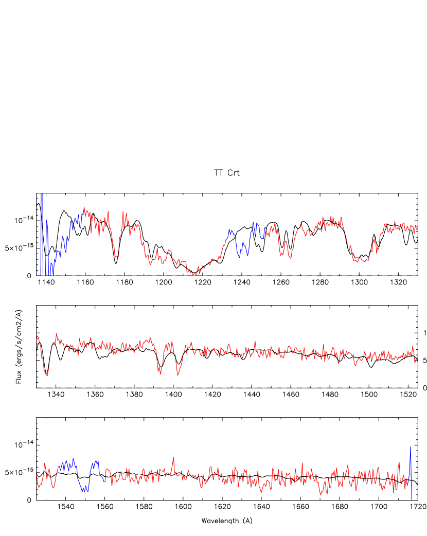
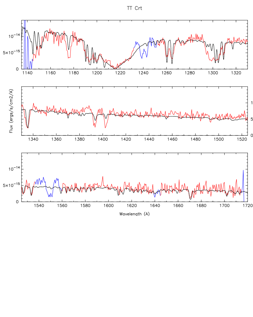
Figure 25: (a) Above. Fitting all the absorption lines simultaneously in the STIS spectrum of TT Crt with a WD model gives a metal abundance [Z]=5 solar with a broadening velocity of 400 km/s. See text for details. (b) Below. Fitting a WD plus an iron curtain helps improve the fit in some regions but degrades the fit in the C iii ($\sim$1175) line and Si (1300) feature. The (WD and iron curtain) abundances are subsolar: [C]=0.01, [Si=0.1], [P]=0.01, and [S]=0.1. The addition of the iron curtain significantly improves the fit in the longer wavelengths (lower panel) and does not produce the C i (1325 & 1330) and Si iii (1343 & 1360) absorption lines which are not present in the STIS spectrum. See text for details.

5.10 V442 Centauri

The STIS snapshot spectrum of V442 Cen, except for the characteristic hydrogen Ly$\alpha$ absorption, and N v ($\sim$1240) and C iv ($\sim$1550) broad emission lines, is rather featureless. It exhibits only three shallow absorption lines: Si ii ($\sim$1260), C ii ($\sim$1335), and Si iii ($\sim$1502).

We carry out a spectral fit without a second component or an iron curtain, first with our grid of solar abundance models, to find the temperature and gravity. The spectral fit results (Fig.26a) give a WD temperature of $31,032\pm 308$ K, and gravity $log(g)=8.042\pm 0.117$. The above-mentioned three shallow absorption lines can be fitted with nearly solar abundances as can be seen in Fig.26, but such a model presents additional strong absorption lines of C iii ($\sim$1175), S ii ($\sim$1250), Si ii (1265), C ii (1330, 1335), Si iv ($\sim$1400), which are not detected in the STIS spectrum.

We note, however, that in Fig.26a the Ly$\alpha$ profile is rather poorly fitted. The bottom of the Ly$\alpha$ goes down to zero in the observed spectrum with what seems to be some possible sharp emission or noise in the middle. At such a high temperature, one does not expect the bottom of the Ly$\alpha$ to go down to zero. The reddening toward V442 Cen is $E(B-V)=0.048\pm 0.015$, while this is still rather small, we decided to check how the ISM absorption affects the Ly$\alpha$ profile. We use the relation of Bohlin et al. (1978) and derive a hydrogen column density of $\approx 3\times 10^{20}$cm^-2 from the value of the color excess $E(B-V)$. We then include modeling of the ISM absorption (as described in Godon et al., 2007) taking $N(H_{\rm I}+N_{2})=3\times 10^{20}$cm^-2, a turbulent velocity of 50km/s and a temperature of 170 K. This modeling does not include metals, but only hydrogen absorption. We find that we can better fit the bottom of the Ly$\alpha$ (bringing it to zero), but we can only fit the right wing of the Ly$\alpha$ profile. The left wings of the profile itself seems to be affected by some weak emission (near 1205 Å), as it slope is steeper than that of the right wing. We include the ISM modeling in the next step: modeling the absorption lines, or rather modeling the absence of absorption lines.

The fit (Fig.26b) to the absence of absorption lines (i.e. neglecting the shallow lines) gives a very small abundance of carbon and silicon: [C]=0.001, [Si]=0.01, with [Z]=1.0 (in solar units), and a rotational broadening velocity of 250 km/s. The broadening velocity could be much smaller for a much smaller metallicity (of all metals), or could be larger too. Since we do not really fit a line, but rather the absence of lines, we cannot derive the projected stellar rotational velocity. As discussed for SDSS 1538, the Si ii (1260) and C ii (1335) absorption lines are likely from the ISM, or from a very thin iron curtain (for C ii (1335)). As to the the Si iii (1502) absorption line, its origin is less clear. Again, as for SDSS 1538, the precise origin of these 3 lines does not change our main result for the WD low abundances of carbon and silicon.

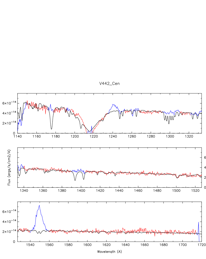
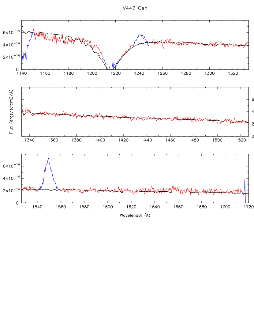
Figure 26: (a) Above. The fit (in black) to the STIS spectrum (in red) of V442 Cen yields a WD temperature $T_{\rm wd}=31,032\pm 308$ K with a gravity $log(g)=8.042\pm 0.117$, for a distance $d=348\pm 5$ pc, reddening $E(B-V)=0.048\pm 0.015$. This model has solar abundances and a broadening velocity of 400 km/s. The model has many absorption lines that are not seen in the data, implying a low metallicity. (b) Below. The the same as above in Fig.26a, but now the abundance of carbon has been lowered to $10^{-3}\times$ solar, and that of silicon is 0.01, with a broadening velocity of $V=250$ km/s. The dotted line represents the WD model only, the solid black line includes ISM absorption modeling affecting the Ly$\alpha$ profile. The Gaia distance to V442 Cen is $348\pm 5$ pc.

6 Summary, Further Considerations and Conclusions

In Table 3 we recapitulate the model fit assumptions made for each of the ten systems.

Except for SDSS 1035, the temperature and gravity ($T,log(g)$) were modeled assuming solar abundances for different values of $E(B-V)$, with and/or without iron curtain, with and/or without a second component as indicated. The major absorption lines were masked as indicated in the Figures. For SDSS 1035, $T$ and $log(g)$ were first assessed assuming solar abundance (for $E(B-V)=0.0$), then they were re-assessed assuming $Z=0.03$ (for $E(B-V)=0.000$ and 0.034).

For all the 10 systems, the abundances [Z] and broadening velocities $V$ were assessed for the best-fit $T,log(g)$ found with a second component where needed, for one value of $E(B-V)$, and without and/or without an iron curtain as detailed in Sec.5.

In column (4) of Table 3: for clarity we did not list all the second component flux values associated with all the reddening values, but a larger reddening yielded a larger second component flux level. In column (5): if there is more than one reddening value, then the value of the second component flux (column 4) and the figures (column 7) are associated with the reddening values annotated with an asterisk $*$ in the same row. Model fits were performed for different reddening values to assess the propagation of reddening uncertainties on the derived temperature and gravity. Since these effects were small, only one reddening value was assumed when deriving abundances and broadening velocities.

Table 3: FUV Spectral Modeling Assumptions, Parameters, and Figures

(1)	(2)	(3)	(4)	(5)	(6)	(7)
System	Exposures	Parameters	2nd Component	$E(B-V)$	Iron	Fig.
Name		Modeled	(erg/s/cm-2/Å)		Curtain
SDSS1035	Combined	$T,log(g)$	—	0.000	No
	Combined	$T,log(g),[Z],V$	—	0.000∗,0.034	No	13,A27
SDSS1538	Combined	$T,log(g)$	—	0.010∗,0.020	No	11,A28
	4th	[Z], $V$	—	0.010	No	12
IY UMa	2nd	$T,log(g)$	$2.5\times 10^{-16}$	0.000∗,0.030	No	15a
	2nd	$T,log(g),[Z],V$	$2.5\times 10^{-16}$	0.000	Yes	15b,A29
DV UMa	Snapshot	$T,log(g)$	$1.16\times 10^{-16}$	0.000∗,0.020	No	16a,A30
	Snapshot	$T,log(g)$	$1.16\times 10^{-16}$	0.000	Yes	16b
	Snapshot	$T,log(g),[Z],V$	$1.16\times 10^{-16}$	0.000	Yes	17
IR Com	1+2+3+5	$T,log(g),[Z],V$	$3.5\times 10^{-16}$	0.019∗,0.041	No	18a
	1+2+3+5	$[Z],V$	$3.5\times 10^{-16}$	0.019∗,0.041	Yes	18b
	1+2+3+5	$T,log(g)$	$3.85\times 10^{-16}$	0.030	No	A31
GY Cnc	Snapshot	$T,log(g)$	$2.0\times 10^{-15}$	0.010∗,0.036	No	19a
	Snapshot	$T,log(g)$	$2.0\times 10^{-15}$	0.010∗,0.036	Yes	19b,A32
	Snapshot	$[Z],V$	$2.0\times 10^{-15}$	0.010	Yes	20
BD Pav	Combined	$T,log(g)$	—	0.039∗,0.075	No	21a,A33
	Combined	$T,log(g),[Z],V$	$7.0\times 10^{-16}$	0.039	Yes	21b
HS2214	Combined	$T,log(g)$	$1.5\times 10^{-15}$	0.029,0.052∗	No	22,A34
	2nd	$[Z],V$	$1.5\times 10^{-15}$	0.052	No	23a
	4th		$1.5\times 10^{-15}$	0.052	No	23b
TT Crt	Snapshot	$T,log(g)$	—	0.012∗,0.029	No	A35
	Snapshot	$T,log(g),[Z],V$	$5.0\times 10^{-16}$	0.012	No	24,25a
	Snapshot	$[Z],V$	$5.0\times 10^{-16}$	0.012	Yes	25b
V442 Cen	Snapshot	$T,log(g)$	—	0.033,0.063∗	No	26a,A36
	Snapshot	$[Z],V$	—	0.063	No	26b

6.1 WD Masses and Temperatures.

In Table 4 we list the WD temperature and gravity for the 10 objects analyzed here, together with the corresponding WD mass and radius, which we derive using the mass-radius relation for non-zero temperature C-O WD from Wood (1995). For comparison, we also list the WD masses that were derived from the eclipse light curves available for 4 systems (SDSS 1035, IY UMa, DV UMa, and GY Cnc; Savoury et al., 2011; McAllister et al., 2019). Except for GY Cnc, we find that our FUV-analysis-derived WD masses agree with the eclipse-light-curve-derived WD masses within the error bar (1-$\sigma$). For GY Cnc the mass (or $log(g)$) agrees within 2.6$\sigma$. At the time of completion of this work, we were also able to compare our WD masses and temperature with the work of Pala et al. (2021) for 6 systems. For comparison, we list In Table 4 the temperatures and WD masses obtained by Pala et al. (2021). This enables us to confirm the results for 3 more systems: SDSS 1538, IR Com and V442 Cen for which we also find good WD mass agreement within the error bars.

While the WD mass we found for SDSS 1035 agrees well with that derived from eclipse light curve, it does not agree with that derived by Pala et al. (2021). A possible explanation for the discrepancy is that Pala et al. (2021) includes a second component in the modeling of SDSS 1035, while we do not find this necessary. Another disagreement, though of less importance, is that for V442 Cen we obtained a temperature about 1200 K higher than Pala et al. (2021). We recall, however, that we included ISM modeling due to the Ly$\alpha$ going down to zero, while the HST spectrum in Pala et al. (2021) does not appear to go down to zero in that region. We use the data calibrated by calcos from mast and Pala et al. (2021) likely re-calibrated the data differently. Furthermore, they do not take into consideration possible absorption from the ISM.

For the rest, our results for $T_{\rm wd}$ and $M_{\rm wd}$ agree within the error bars with the results of Pala et al. (2021). Small differences are likely due to the different versions of tlusty (203 vs. 204n), and the running parameters we use in synspec such as for the NLTE approximation at high temperature and convection at low temperature. We also use different prescriptions for the hydrogen quasi-molecular satellite lines opacity. Furthermore, the second component and the absorbing curtains are treated differently; the dereddening, masking, and calibration of the spectra are also performed differently. However, overall, our results and Pala et al. (2021)’s results confirm each other (Pala, 2021).

The reason for the poor agreement found for GY Cnc with the elicpse light curve WD mass may be due to the strong veiling. GY Cnc is the system the most affected by veiling after IY UMa. Its modeling required an iron curtain with a hydrogen column density of $5\times 10^{21}$cm^-2, 10 times larger than for TT Crt. It is worth noting also that GY Cnc is the object for which McAllister et al. (2019) obtained the largest discrepancy (2$\sigma$) for the derived distance based on their WD atmosphere fit: they obtained a distance of 320 pc with a WD temperature of $\sim 25,900$ K. The exact reasons for the WD atmosphere fit discrepancies in the present work and in McAllister et al. (2019) are not known, but, in addition to strong veiling, GY Cnc has a prominent bright spot and its HST STIS spectrum was obtained a few weeks only after outburst. We further emphasize that this is the first attempt to model the HST FUV spectrum of GY Cnc and that this object was excluded from all previous analyses (by us and by others).

We can therefore confirm that FUV spectral fits supplemented with Gaia distances provide a robust method to derive CV WD masses and temperatures and open the path to constraining the evolution of CVs (Pala et al., 2021).

Table 4: FUV Spectral Analysis Results: WD Masses and Temperatures

(1)	(2)	(3)	(4)	(5)	(6)	(7)	(8)	(9)
System	$T_{\rm wd}$	Pala et al. (2021)	$log(g)$	$M_{\rm wd}$	$M_{\rm wd}^{E}$	Pala et al. (2021)	$R_{\rm wd}$	Iron
Name	(K)	(K)		$(M_{\odot})$	$(M_{\odot})$	$(M_{\odot})$	(km)	Curtain
SDSS1035	$11,475\pm 188$	$11,876^{+108}_{115}$	$8.385\pm 0.166$	$0.830^{+0.118}_{-0.102}$	$0.835\pm 0.009$	$1.00^{+0.08}_{-0.10}$	$6740^{-790}_{+890}$	No
SDSS1538	$35,743\pm 576$	$35,284^{+600}_{-688}$	$8.708\pm 0.130$	$1.073^{+0.066}_{-0.074}$		$0.97^{+0.09}_{-0.11}$	$5284^{-600}_{+640}$	No
IY UMa	$17,130\pm 249$	$17,057^{+179}_{-79}$	$8.480\pm 0.125$	$0.903^{+0.090}_{-0.088}$	$0.955^{+0.013}_{-0.028}$	$0.99^{+0.04}_{-0.03}$	$6300^{-575}_{+610}$	Yes
DV UMa	$19,325\pm 481$	$19,410^{+244}_{-400}$	$8.565\pm 0.177$	$0.968^{+0.116}_{-0.127}$	$1.09\pm 0.03$	$0.96^{+0.07}_{-0.10}$	$5910^{-820}_{+850}$	Yes
IR Com	$17,860\pm 180$	$17,531^{+236}_{-271}$	$8.613\pm 0.090$	$1.001^{+0.055}_{-0.066}$		$1.03^{+0.07}_{-0.09}$	$5690^{-420}_{+410}$	Yes
GY Cnc	$22,515\pm 292$		$7.876\pm 0.108$	$0.570^{+0.050}_{-0.050}$	$0.881\pm 0.016$		$10043^{-800}_{+830}$	Yes
BD Pav	$19,330\pm 312$		$8.117\pm 0.158$	$0.683^{+0.087}_{-0.083}$			$8320^{-960}_{+1035}$	Yes
HS2214	$27,643\pm 268$		$8.301\pm 0.160$	$0.798^{+0.108}_{-0.086}$			$7260^{-810}_{+1020}$	No
TT Crt	$26,990\pm 557$		$8.044\pm 0.097$	$0.663^{+0.049}_{-0.049}$			$8910^{-645}_{+690}$	Yes
V442 Cen	$31,032\pm 308$	$29,802^{+211}_{-247}$	$8.042\pm 0.117$	$0.671^{+0.057}_{-0.057}$		$0.64^{+0.06}_{-0.05}$	$8980^{-785}_{+870}$	No

Note. — In column (2) we list the WD temperatures from our spectral analysis, followed in column (3) by the WD temperatures from Pala et al. (2021). In column (5) we list the WD masses obtained from our spectral analysis together with the WD masses derived from eclipse light curves (6) (Savoury et al., 2011; McAllister et al., 2019) and from Pala et al. (2021) (7). The masses (5) and radii (8) were computed from the values of $log(g)$ (4) using the mass-radius relation for non-zero temperature WD (Wood, 1995). Since for each spectrum the solution is a narrow diagonal band in the $T_{\rm wd}$ vs $log(g)$ parameter space, the larger temperature (+) is associated with the larger gravity (+), larger WD mass (+), and smaller WD radius (-), and vice versa.

6.2 WD Chemical Abundances and Stellar Rotational Velocities.

The abundances analysis, summarized in Table 5, reveals that only two systems (IY UMa and HS 2214) have a WD spectrum consistent with solar carbon abundance [C]=1. Seven systems have [C]$\sim$0.1-0.0001, 6 have subsolar silicon ([Si]$\sim$0.1-0.01), and 4 have [P]$\lesssim$0.01 and [S]$<$1. Of all the 10 systems, only IY UMa has solar metal abundances ([C]=[Si]=[Z]=1; see also below). IR Com is considered separately in Sec.6.4.

All the dominant absorption lines in the spectra are due to carbon and silicon, which makes the determination of the abundance of these species more reliable. The low abundance of P was based solely on the absence of the single line P ii (1452.89) in the observed spectra which forms in the iron curtain models. The S abundance was based solely on the sulfur doublet near $\sim 1250$.

Except for the N v ($\sim$1240) doublet forming in a hot gas, no strong nitrogen absorption lines were detected in the spectra and nitrogen abundance could not be assessed. Some nitrogen lines do form in the short wavelength region, but are either too shallow to give a reliable measurement (e.g. $\sim 1200$ Å), or are in that region near the edge of the detector and where the iron curtain affects the spectra ($\sim 1140-1160$ Å). Nevertheless, nitrogen was kept solar, just as all the other metals marked in Tables 5 & 6 with [Z]=1.

In Table 5, we list the broadening velocities of the lines from the best fit model for each system. These velocities range from 150 km/s to 400 km/s, these velocities are all sub-Keplerian, similar to the values obtained in earlier studies with HST (Sion, 1999). The velocity $V$ is expected to correspond to the projected WD stellar rotational/spin velocity $V_{\rm rot}sin(i)$ when the lines are not affected by the motion of the WD around the center of mass during the duration of the exposure. We list (column 10) the approximate velocity broadening $V_{\rm WD}$ due to the WD motion around the center of mass during the duration of the observation. For the systems for which the absorption lines are not due to the absorbing slab, one can assume a projected WD rotational velocity $V_{\rm rot}sin(i)\approx V-V_{\rm WD}$. Doing so we obtain $V_{\rm rot}sin(i)$ for SDSS 1035 ($\approx 100$ km/s), SDSS 1538 ($\approx 300$ km/s), IR Com ($\approx 50$ km/s, or less; the size of the velocity uncertainty), HS 2214 ($\approx 375$ km/s), and V442 Cen ($\leq 250$ km/s). For the other systems (IY UMa, DV UMa, GY Cnc, BD Pav, TT Crt), where the absorption lines are due mainly to the iron curtain, the resulting velocity $V-V_{\rm WD}$ is more representative of the actual broadening of the absorption lines in the veiling material, which depends on both the turbulent velocity and column density (see next subsection).

Table 5: FUV Spectral Analysis Results: Abundances and Velocities

(1)	(2)	(3)	(4)	(5)	(6)	(7)	(8)	(9)	(10)	(11)
System	[C]	[Al]	[Si]	[P]	[S]	[Fe]	[Z]	$V$	$V_{\rm WD}$	N h
Name	($\odot$)	($\odot$)	($\odot$)	($\odot$)	($\odot$)	($\odot$)	($\odot$)	(km/s)	(km/s)	($10^{20}$cm-2)
SDSS1035	$0.03\pm 0.02$						$0.03\pm 0.02$	$150\pm 50$	57	—
SDSS1538	$\sim 10^{-4}$		$1_{-0.5}^{+1}$				1.0	$400\pm 100$	$\sim$100	—
IY UMa				$\lesssim 0.01$			1.0	$150\pm 50$	44	100
DV UMa	$0.1_{-0.05}^{+0.1}$		$0.3\pm 0.1$	$\lesssim 0.01$	$\lesssim 1.0$		1.0	$150\pm 50$	40	20
IR Com	$1.0_{-0.5}^{+1.0}$	$5\pm 1$	$1\pm 0.5$			$4\pm 1$	1.0	$150\pm 50$	154	—
IR Com	$0.4\pm 0.1$						1.0	$150\pm 50$	154	$\lesssim 0.1$
GY Cnc	$0.01_{-0.005}^{+0.01}$		$0.1_{-0.05}^{+0.10}$	$\lesssim 0.01$	$0.1_{-0.05}^{+0.10}$		1.0	$150\pm 50$	28	50
BD Pav	$0.01_{-0.005}^{+0.01}$	$0.1_{-0.05}^{+0.10}$	$0.1_{-0.05}^{+0.10}$	$\lesssim 0.01$	$\lesssim 1.0$		1.0	$200\pm 50$	190	10
HS2214			$0.2\pm 0.1$				1.0	$400\pm 50$	$\sim$26	—
TT Crt	$0.01^{+0.01}_{-0.005}$		$0.1^{+0.10}_{-0.05}$	$\lesssim 0.01$	$0.1^{+0.10}_{-0.00}$		1.0	$400\pm 100$	25	5
V442 Cen	$\lesssim 0.001$		$\lesssim 0.01$				1.0	$\gtrsim 250$	$\sim$10	—

Note. — When a specific absorption line was used to model the abundance of a given element, the resulting abundance is written directly the column of that element. The remaining of the chemical elements were set to the value listed in column (8) marked with [Z]. In column (9) we list the broadening velocity of the absorption lines from the analysis. In column (10) we list the approximate velocity broadening due to the motion of the WD around the center of mass during the time the exposure was obtained, computed using the $K_{1}$ values (see Table 1; assumed to be 100 km/s if unknown) and the ratio of the exposure time (Table 2) to the orbital period (Table 1). In the last column (11) we indicate the hydrogen column density of the iron curtain. Assuming that IR Com is affected by an iron curtain implies that the WD photospheric abundances are all solar (1x), except carbon (0.4x), for that reason results are shown with and without an iron curtain - see text for a detailed discussion.

6.3 The Iron Curtain.

The effect of veiling material is obvious in IY UMa, DV UMa, GY Cnc, and BD Pav, and, while less noticeable, it is still detectable in TT Crt. For these 5 systems, the abundances were derived using an iron curtain masking the WD, and assuming that the WD and iron curtain have the same abundances. The iron curtain models are listed in Table 6 for each veiled system.

In the iron curtain modeling, we first fitted the forest of iron lines in the longer wavelengths assuming solar iron abundance for the curtain (and WD). We then found that even low abundances of C, Si, S,.. ($<<1$ solar) in the curtain generate deep and wide absorption lines, which forced us to reduce these abundances to subsolar. Since we assumed that the WD and iron curtain had the same abundances, we reduced the WD photosphere C, Si, S, .. abundances as well, which removed from the model lines that were not observed (sulfur lines at $\sim$1250 Å, silicon lines at 1260,1265 Å, $\sim$1340 Å, $\sim$1360 Å, carbon lines at $\sim$1330 Å, etc..; these lines do not form in the iron curtain). Therefore, our assumption that the WD and iron curtain have the same abundances is self-consistent. We did not change, however, the iron abundance in the curtain and kept it to solar, since it is used to match the iron forest in the longer wavelengths and derive the iron curtain basic parameters (turbulent dispersion velocity and hydrogen column density).

Assuming solar iron abundance for the iron curtain is reasonable, but may introduce an uncertainty. While the iron abundance in a CV WD or secondary star cannot be large enough to produce the kind of Fe ii absorption lines seen in the FUV spectra of these 5 systems, the iron abundance of stars (at all age [0-10 Gyr]) in the solar neighborhood shows a scatter of [Fe/H] abundances of up to about $\pm 0.5$ dex (Rebassa-Mansergas et al., 2021). Metal-rich ([Fe/H] $\sim 0.2$ dex or 1.6$\times$solar) and super-metal-rich ([Fe/H] $\sim 0.5$ dex, or 3.2$\times$solar) stars in the solar neighborhood are not distinct in terms of their kinematics or ages, and seem to form a continuous distribution; this does not exclude that some of the super-metal-rich stars in the solar neighborhood might originate from the inner disk and even the Galactic bulge (Feltzing & Chiba, 2013). Therefore, we do not expect the iron abundance in a CV WD to be larger than $\sim 3\times$solar, and the probability of it reaching $\sim 3$ is certainly very small. It is more likely that the iron abundance in a CV WD is nearly 1. Consequently, the abundances of C, Al, Si, P, and S derived from the solar [Fe/H] assumption in the iron curtain (Table 6) is a good assumption and would be (in the extreme case) accurate to within a factor not exceeding $\sim 3$ ($\sim 0.5$ dex).

Table 6: Iron Curtain Modeling Parameters

System	N h	$V_{\rm turb}$	[C]	[Al]	[Si]	[P]	[S]	[Z]
Name	(cm-2)	(km/s)	$\odot$	$\odot$	$\odot$	$\odot$	$\odot$	$\odot$
IY UMa	$1\pm 0.2\times 10^{22}$	75${}_{-15}^{+25}$				$\lesssim 0.01$		1.0
DV UMa	$2\pm 1\times 10^{21}$	75$\pm 25$	0.1		0.3	$\lesssim 0.01$	$\lesssim 1$	1.0
IR Com	$\lesssim 1\times 10^{19}$	100$\pm 25$	0.4					1.0
GY Cnc	$5\pm 2\times 10^{21}$	75$\pm 25$	0.01		0.1	$\lesssim 0.01$	0.1	1.0
BD Pav	$1\pm 0.3\times 10^{21}$	200$\pm 50$	0.01	0.1	0.1	$\lesssim 0.01$	$\lesssim 1$	1.0
TT Crt	$5\pm 2\times 10^{20}$	100$\pm 25$	0.01		0.1	$\lesssim 0.01$	0.1	1.0

Note. — All the iron curtain models here have the same temperature ($T=10,000$ K) and electron density ($n_{e}=10^{13}$cm^-3) as in Horne et al. (1994), and iron is set to solar ([Fe]=1). The error bars on the abundances are the same as for the WD in Table 5. Here too, when a specific absorption line was used to model the abundance of a given element, the resulting abundance is written directly the column of that element. The remaining of the chemical elements were set to the abundance in the column marked with [Z].

It is true that a single isothermal iron curtain model with a given electron density, hydrogen column density, and turbulent velocity is only an approximation, since the veiling material is made of a gas that is not especially isothermal, nor has a constant density, nor a constant turbulent velocity. As such, we do not expect the fit to be perfect and the iron curtain only comes to improve the WD fit. Furthermore, one has to be aware that a lower iron curtain density requires a lower iron curtain temperature for the iron features to form and the hydrogen column density inversely correlates with the turbulent velocity to match the strength of the curtain absorption features in the final spectrum (Horne et al., 1994).

The low carbon abundance we found in 7 systems cannot be due to the iron curtain simplistic modeling, since for the systems that did not include an iron curtain modeling, we find 3 systems out of 5 also have a low carbon abundance (for the systems with an iron curtain we find 4 out of 5 with a low carbon abundance). The same is true for the low silicon abundance. However, the same cannot be said of the low phosphorus abundance. The P ii ($\sim$1453) absorption line only appeared in the iron curtain modeling and no P lines appear in the WD stellar model. Since none of the 10 HST WDs spectra analyzed here exhibit the P ii absorption line, we cannot rule out that the P ii line is the product of an inaccurate iron curtain modeling, albeit able to reproduce all the other spectral features due to C, Al, Si, S, and Fe. More iron curtain modeling is needed, as well as a rigorous inspection of all the CV WDs FUV spectra available to determine whether this line is the sole product of an inaccurate iron curtain modeling or whether it is also an observed feature.

We note that the absorbing slab turbulent velocity listed in Table 6 does not especially correspond to the broadening velocity of the absorption lines in the veiling material, since the broadening of the iron curtain lines (for a given temperature and electron density) depends also on the hydrogen column density. For that reason, and except for IR Com where most of the lines are from the WD photosphere, we cannot derive the projected rotational stellar velocity for the systems listed in Table 6.

6.4 The Thin Iron Curtain: IR Com with or without a Mask?

In a system like HS 2214+2845, the spectra reveal stronger absorption lines as well as the appearance of new lines at orbital phases $\sim 0.0$, 0.31, and 0.64, but not when the WD is facing the observer near orbital phase 0.5. While it is known that veiling material, likely due to the L1-stream overflowing the edge of the disk, can affect the spectrum at orbital phases near 0.25 and 0.6-0.8 (see Godon, 2019, and references therein), it is not clear that some partial veiling does not take place at other orbital phase or even in systems with a low inclination.

From the IR Com thin iron curtain ($N_{\rm H}=10^{19}$cm^-2) modeling, we find that seemingly one cannot differentiate between a thin curtain veiling a solar abundances (with [C]=0.4 solar) WD photosphere and a non-veiled WD photosphere with increased (supra-solar) aluminum ([Al]$\sim$5) and iron ([Fe]$\sim$4) abundances. Both produce the observed Al ii lines and Fe ii saw tooth pattern (in the longer wavelengths). The question then arises as to whether IR Com should be modeled with or without a mask. However, first, for reason we explained above, it is unlikely that iron abundance in the WD or donor star is larger than 3 (in solar units), and, second, these Al and Fe absorption features were observed in U Gem at orbital phases $\Phi=0.25,0.67-0.81$ and were attributed to veiling material (Godon et al., 2017, note that the line identified as a WD argon line in that work is actually the Al ii 1670.79 Å  curtain line). Consequently, we conclude that the WD in IR Com has Al and Fe solar abundances and is veiled by a thin iron curtain.

6.5 Conclusion.

We confirm that with the availability of accurate Gaia distances, FUV spectral fits provide a new tool to derive the WD mass and temperature in CVs, even for systems where the WD is significantly veiled. We made the assumption that the veiling material and the WD have the same abundances, and found that this assumption is self-consistent. Overall, our results further strengthen previous findings that DNe in quiescence have WDs with subsolar abundances of carbon and silicon, as well as possibly subsolar abundances of phosphorus and sulfur. All the derived projected stellar rotational velocities we found are well below the Keplerian break-up velocities. We also raise the possibility that WD suprasolar abundance of aluminum, nitrogen and iron, derived from fitting FUV absorption lines in some systems, may rather be due to the presence of a thin iron curtain. Alas, nitrogen abundance could not be derived to assess the N/C ratio, as dominant nitrogen lines only form at shorter wavelengths, requiring FUSE or e.g. COS FUV G140L (1280 Å) spectral analyses. At these wavelengths ($\lambda<1170$ Å) veiling material can also produce strong absorption bands of Fe ii as well as deeper absorption lines of nitrogen, making such a task more challenging.

The analysis of CV white dwarf metal abundances and their implications represents a relatively new frontier in CV white dwarf research. The principal objective is to determine the abundances of accreted metals for a statistically significant large sample of CVs. Overabundances of metals especially, odd-numbered species like aluminum and phosphorus are built up through proton captures outside the explosive CNO Bi-Cycle burning of past nova-explosions, contaminating the donor star during the nova common envelope stage which envelops the donor star (Sion & Sparks, 2014; Sparks & Sion, 2021). Whether this process is responsible for the N/C composition anomaly, or whether metal overabundances were carried over by the WD after the AGB thermal pulsing stage, these nuclei are likely the ancient relics of hot CNO Burning.

Appendix A The $\chi^{2}$ Maps

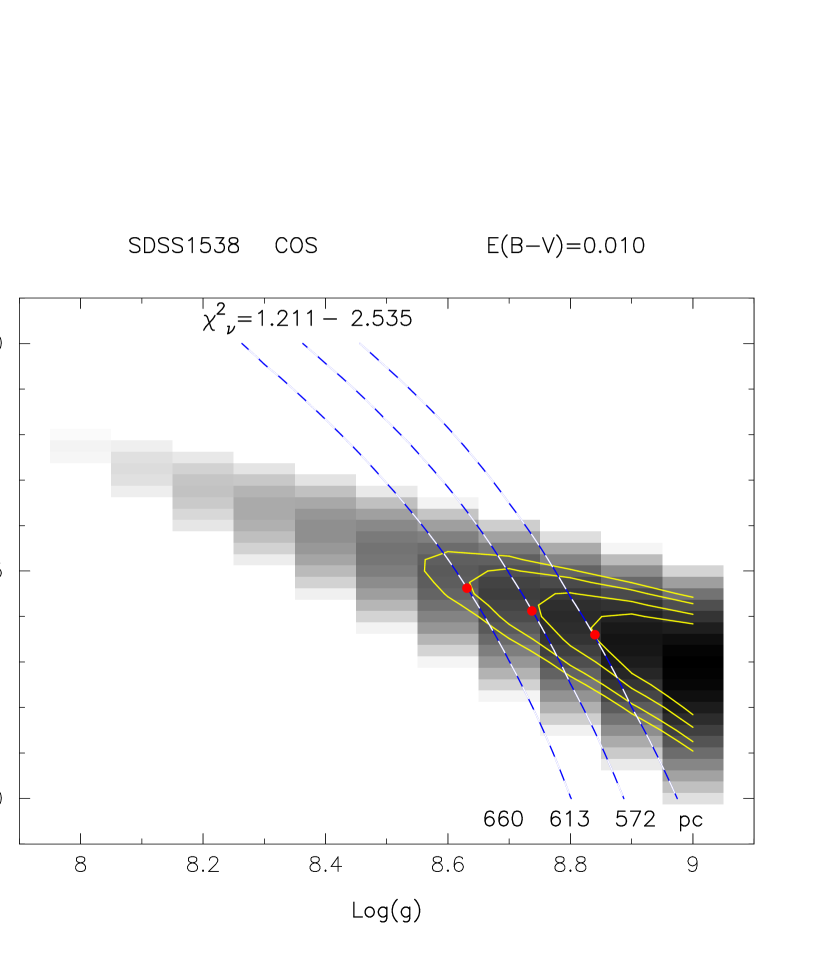
Figure 28: The $chi^{2}$-map of the modeling of the COS spectrum of SDSS 1538 (CRTS J153817.3+512338) is shown assuming $E(B-V)=0.01$. The least $\chi^{2}_{\nu}$ model scaling to the Gaia distance of 613 pc yields $log(g)=8.74$ and $T_{\rm wd}=35,875$ K (middle red spot). The solutions are also shown for upper (left red spot) and lower (right red spot) limits of the Gaia distance.

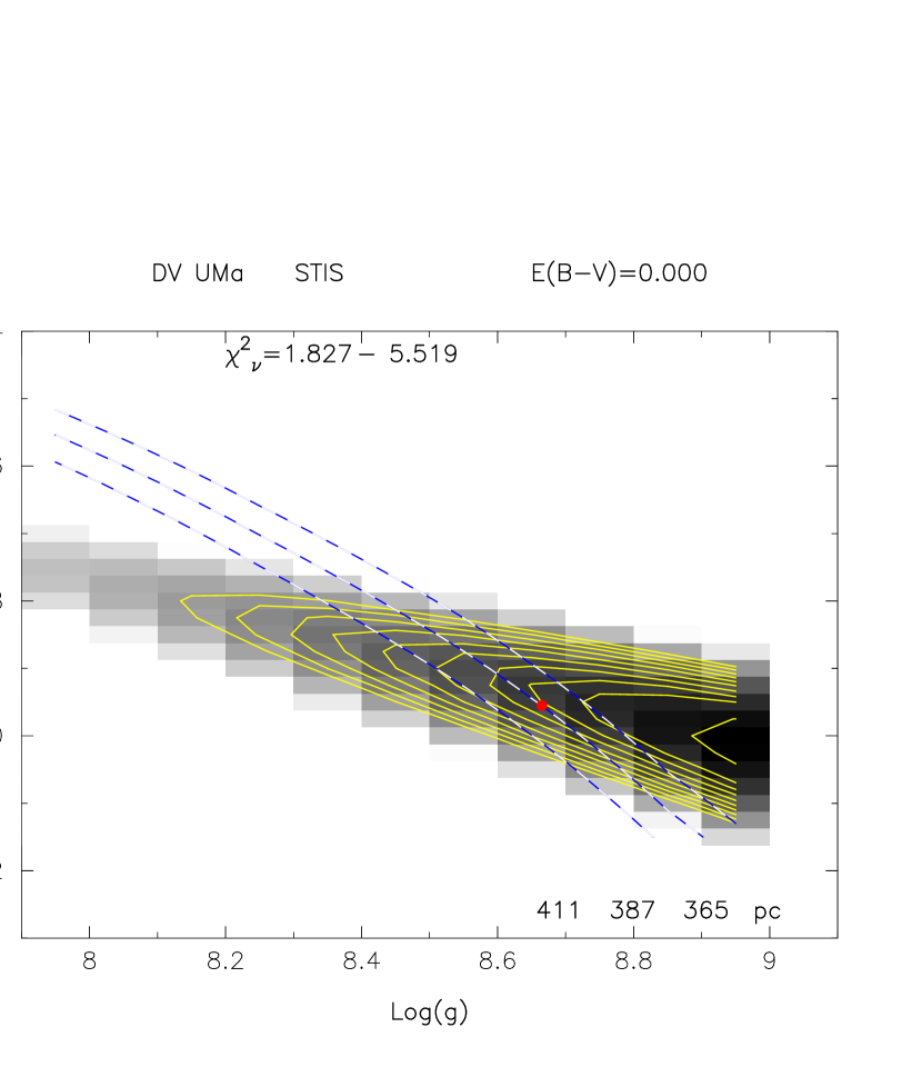
Figure 30: The $\chi^{2}$-map of the fitting of the STIS spectrum of DV UMa is shown assuming $E(B-V)=0$ and including a second flat component. The solution for the Gaia distance of 387 pc is marked with the red dot: $T_{\rm wd}=20,050$ K with $log(g)=8.715$.

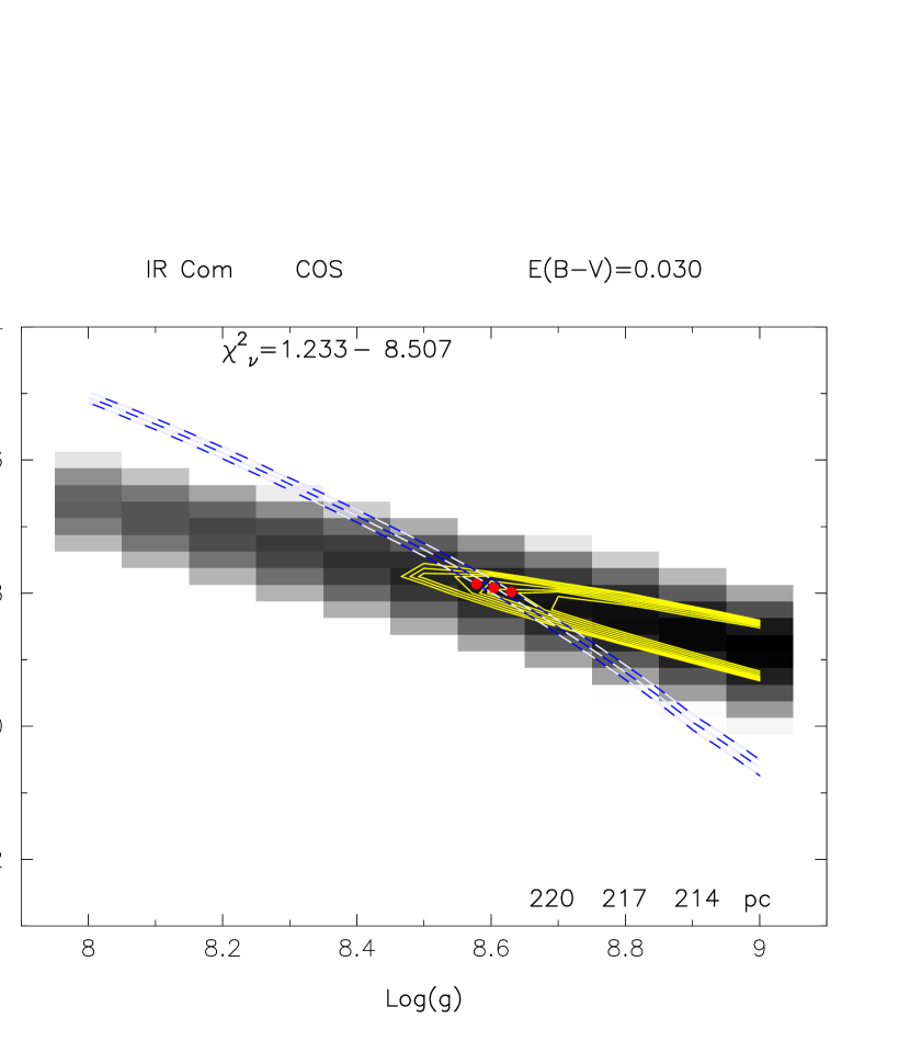
Figure 31: The $\chi^{2}$-amp of the results of the spectral fit to the COS spectrum of IR Com is presented assuming $E(B-V)=0.03$ and a second flat component. The models fitting the Gaia distance ($\pm$error) are found along the triple blue dashed line and achieve a minimum $\chi^{2}_{\nu}$ denoted by the three red dots.

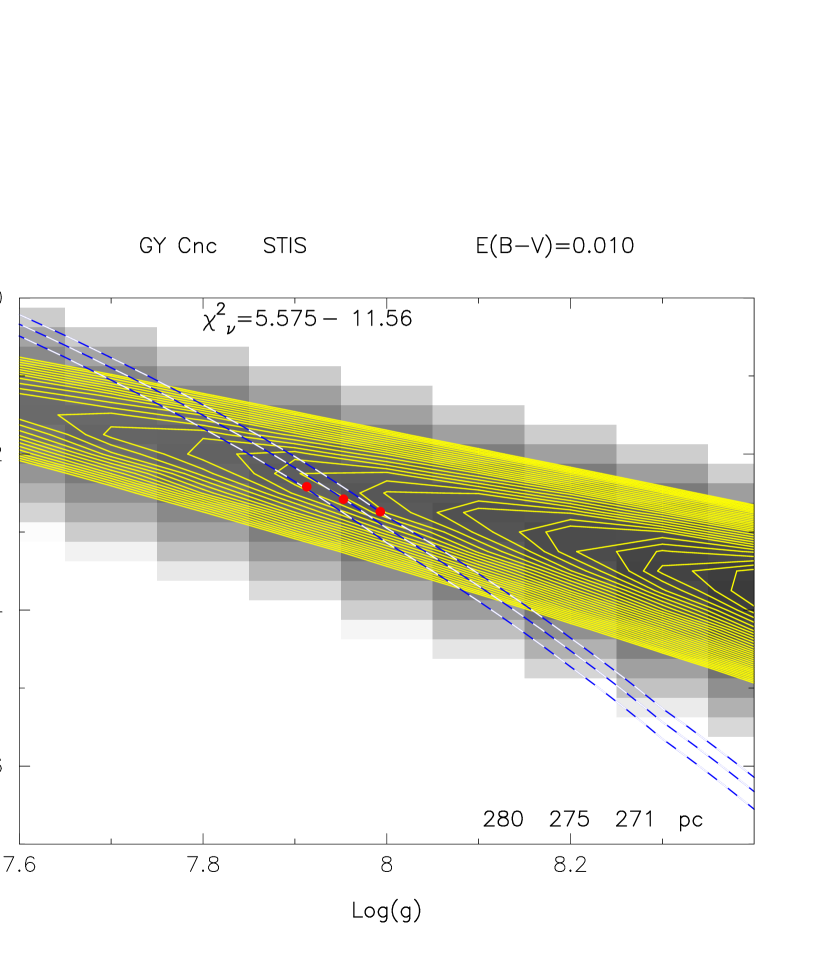
Figure 32: The results of the fitting of the STIS spectrum of GY Cnc with a veiled WD model spectrum is displayed as a map of the $\chi^{2}_{\nu}$ value in the $log(g)$ vs. decreasing $T_{\rm wd}$ parameter space. We assume a reddening of $E(B-V)=0.010$ and include a second flat component as well as an absorbing slab.

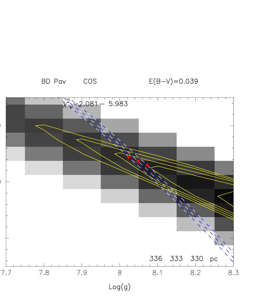
Figure 33: The results of the first step in the modeling of the COS spectrum of BD Pav are shown as a map of the $\chi^{2}_{\nu}$ in the parameter space $T_{\rm wd}$ vs. $log(g)$. No second component and no iron curtain are included in this first step, the spectrum was dereddened assuming $E(B-V)=0.039$. The best fit scaling to the Gaia distance yields $log(g)=8.048$ and $T_{\rm wd}=19,630$ K (middle red spot). After the inclusion of a second component and an absorbing slab, and taking into account the upper limit of the reddening ($E(B-V)=0.075$), the best fit temperature and gravity change noticeably (see the results section).

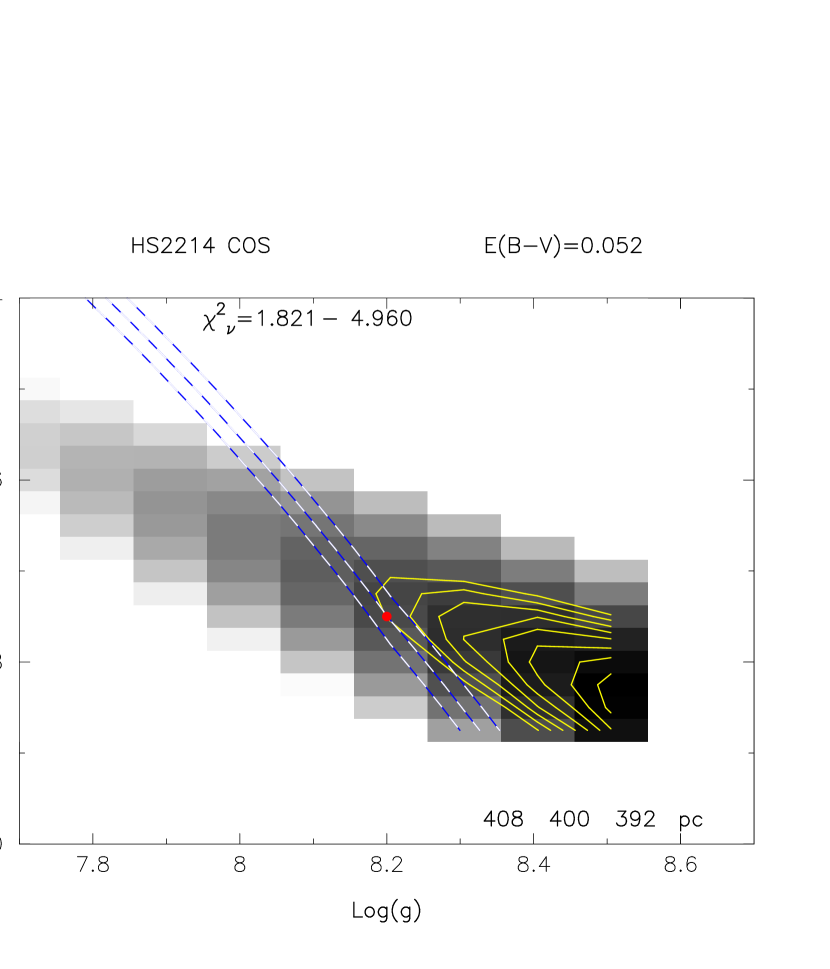
Figure 34: The results of the spectral fit of the COS spectrum of HS 2214+2845, assuming a reddening of $E(B-V)=0.052$,are summarized in this map of the values taken by the reduced $\chi^{2}_{\nu}$. The least chi square along the line d=400 pc gives the solution $T_{\rm wd}=27,500$ K with $log(g)=8.20$ (red dot). Note that the distance lines (blue dashed lines) achieve a minimum $\chi^{2}_{\nu}$ slightly off the center of the gray diagonal.

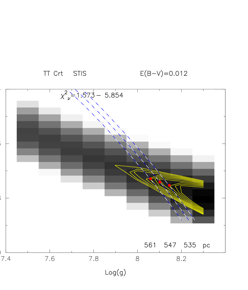
Figure 35: The $\chi^{2}$-map of results of the spectral fit of the STIS spectrum of TT Crt is displayed assuming $E(B-V)=0.012$. The least chi square along the line d=547 pc gives the solution $T_{\rm wd}=27,290$ K with $log(g)=8.102$ (middle red dot).

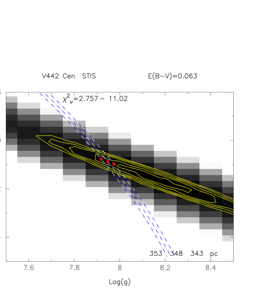
Figure 36: The $\chi^{2}$-map of the spectral fit to the STIS spectrum of V442 Cen assuming E(B-V)=0.063 is displayed. Solar abundances were assumed in the modeling, which did not include a second component nor an absorbing slab.

We generate a grid of WD model spectra in a confined region of the gravity-temperature parameter space, ranging from $log(g)=7.5$ to $log(g)=9.0$ and $T_{\rm wd}=10,000$ to $T_{\rm wd}=40,000$, in steps of 250 K in temperature and $0.1$ in gravity ($log(g)$). In order to derive the WD temperature and gravity, each HST spectrum is fitted against a portion of this grid, a subgrid, typically including approximately 100 to 400 WD models. For each single model fit (with a given WD temperature and gravity) within a subgrid, a $\chi^{2}_{\nu}$ value as well as a scaling distance is obtained. The results for all the model fits within that subgrid, i.e. for a given DN system, are then summarized as a map of $\chi^{2}_{\nu}$ in the parameter space $log(g)$ vs. $T_{\rm wd}$. Such a $\chi^{2}$-map is used to visually display and derive the best-fit WD model for the Gaia distance. In this section of the Appendix we present such $\chi^{2}$-maps for the 10 DNe systems in Figs.27-36.

In each $\chi^{2}$-map, we draw yellow contour lines of the $\chi^{2}_{\nu}$ values superposed to a gray scale of the least $\chi^{2}_{\nu}$ in the (decreasing) WD effective surface temperature ($T_{\rm wd}$) versus (increasing) WD surface gravity ($log(g)$) parameter space. Each theoretical stellar spectrum model occupies a 250 K $\times 0.1(log(g))$ rectangle area as shown in the figures. For clarity, only the lowest $\chi^{2}_{\nu}$ models are shown with the gray scale (darker indicates smaller $\chi^{2}_{\nu}$) and yellow contour lines, forming a diagonal in the ($log(g),T_{\rm wd}$) parameter space. The range of the $\chi^{2}_{\nu}$ values is indicated in each figure.

Since a distance is also obtained for each model (rectangle), we draw lines of constant distance corresponding to the Gaia distance, including its upper and lower limits: the three blue dashed lines.

In each $\chi^{2}$-map, the temperature of the WD is then found where the $\chi^{2}_{\nu}$ takes a minimum along the Gaia distance line. This minimum is achieved in the region where the blue dashed distance line intersects the least-$\chi^{2}_{\nu}$ gray diagonal and is marked with red dot.

The $\chi^{2}$ maps presented here, however, are only a small sample representative of all the model fits that were run. Only one $\chi^{2}$ map is presented for each DN system, but many more were computed for different values of the reddening and of the second component flux level, as well as for different iron curtain models (where applicable). As such the temperature and gravity solutions displayed here in these $\chi^{2}$-map are not the final results presented in Table 4, but they contributed to them (i.e. the temperature and gravity solutions in the following $\chi^{2}$ are within the error bars of the final results presented in Table 4).

In all the $\chi^{2}$-maps, low $\chi^{2}$ values are obtained on a diagonal starting at a colder temperature at the lower limit of $log(g)$ (near the upper left corner of the maps), and crossing to a hotter temperature at the upper limit of $log(g)$ (near the lower right corner in the maps). This diagonal corresponds to the fitting of the hydrogen Lyman$\alpha$ absorption feature, and is a result of the well-known degeneracy of the solution (e.g. Gänsicke et al., 2005), due to the fact that increasing the temperature and increasing the gravity have opposite effects on the Ly$\alpha$ profile (narrowing vs. broadening, respectively).

We note, however, that 7 of the 10 $\chi^{2}$-maps exhibit the lowest $\chi^{2}$ (absolute minimum, darkest rectangle) at the very end (higher temperature/gravity) of that diagonal. A reasonable cause could be that a “hot” second component (rather than a flat one) is responsible for this effect, but it appears that this effect also occurs in cases where the slope of the observed spectrum is shallower (colder) than the best-fit model, and while such a second component slightly reduces the effect in a system like HS 2214+2815, it does not provide a satisfactory explanation. We also notice that some systems (e.g. DV UMa) exhibit some extra flux in the very short wavelengths ($<1200$ Å), which could partially explain this effect. For IY UMa, the opposite is certainly true: the COS spectrum presents some extra flux on the right wing of Ly$\alpha$ when compared to the models, and the least $\chi^{2}_{\nu}$ is obtained near the low temperature/gravity of the diagonal in its $\chi^{2}$-map. Last, we find the higher temperature/gravity models have in general shallower absorption lines, and since most systems have rather low abundances, a slightly better fit is obtained at higher temperature (in spite of the fact that we mask the dominant absorption feature in the first place). Except for SDSS 1035, all the $chi^{2}$-maps were generated using solar abundance WD models [generating non-solar abundance $\chi^{2}$-map requires generating grid of models for all the different abundances obtained in this work, which would be prohibitively CPU-expensive], and the $\chi^{2}$-map of SDSS 1035 almost does not show that effect. Consequently, we conclude that this effect is most likely a combination of the above causes, and it is further affected by the veiling material strongly masking half of the systems. In any case, the relative difference in the $\chi^{2}_{\nu}$ obtained for the Gaia distance best-fit is only of the order of 1% larger than for the absolute minimum $\chi^{2}_{\nu}$.

A.1 SDSS1035

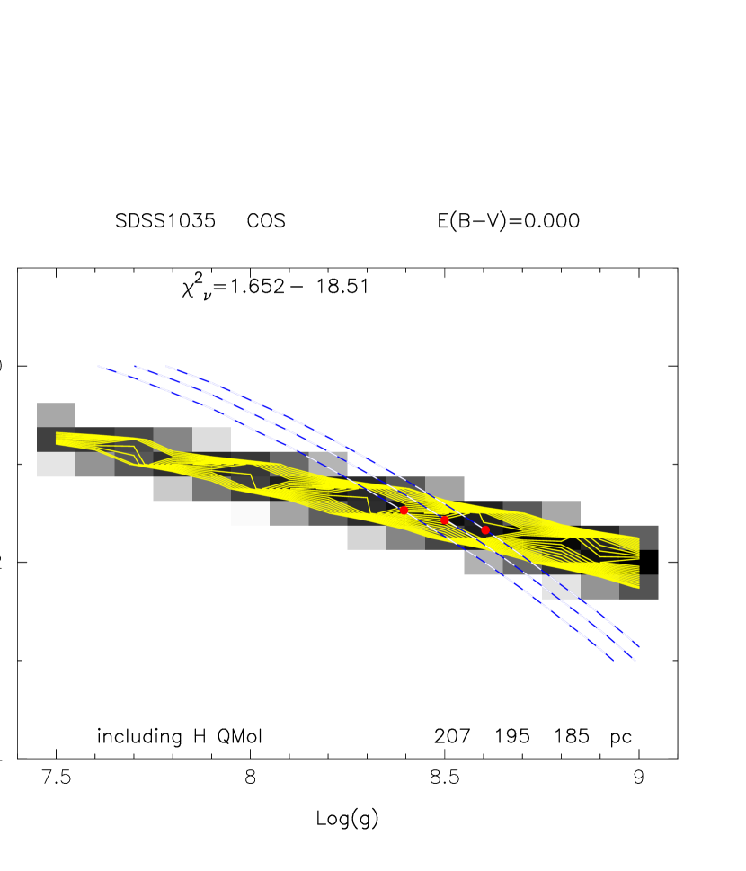
Figure 27: The results of the fitting of the COS spectrum of SDSS 1035 with a WD model spectrum are displayed as a map of the $\chi^{2}_{\nu}$ value in the $log(g)$ vs. decreasing $T_{\rm wd}$ parameter space. For clarity, only the lowest $\chi^{2}_{\nu}$ models are shown with the gray scale and yellow contour lines (darker grey indicates smaller $\chi^{2}_{\nu}$) forming a diagonal. The $\chi^{2}_{\nu}$ value increases from $\sim 1.652$ (within the diagonal) to 18.51 (upper right and lower right corner - in white) as indicated in the panel. The three white-blue dashed lines correspond to the distances: 207 pc (left dashed line), 195 pc (middle dashed line), and 185 pc (right dashed line). The least chi square along the line d=195 pc gives the solution $log(g)=8.50$ and $T_{\rm wd}=11,570$ K (middle red dot). The solution for 207 pc is marked with the left red dot and that for 185 pc is marked with the right red dot. The solution is summarized as $log(g)=8.500\pm 0.105$ with $T_{\rm wd}=11,570\pm 100$ K for a distance $d=195_{+12}^{-10}$ pc. The WD model has a metal abundance of 0.02 solar. The COS spectrum was not dereddened. Similar $\chi^{2}$ maps were also computed by running model fits assuming $E(B-V)=0.034$, and assuming solar abundances (separately).

A.2 SDSS 1538+5123

A.3 IY UMa

A.4 DV UMa

A.5 IR Com

A.6 GY Cnc

A.7 BD Pav

A.8 HS 2214+2845

A.9 TT Crt

A.10 V442 Cen

ORCID iDs

Patrick Godon https://orcid.org/0000-0002-4806-5319
Edward M. Sion https://orcid.org/0000-0003-4440-0551

References

- Avni (1976) Avni, Y. 1976, ApJ, 210, 642
- Bailer-Jones (2015) Bailer-Jones, C.A.L. 2019, PASP, 127, 994
- Bohlin et al. (2014) Bohlin, R.C., Gordon, K.D., Tremblay, P.-E. 2014, PASP, 126, 711
- Bohlin et al. (1978) Bohlin, R.C., Savage, B.D., & Drake, J.F. 1978, ApJ, 224, 132
- Capitanio et al. (2017) Capitanio, L, Lallement, R., Vergely, J.-L. et al. 2017, A&A, 606, 65
- Debes et al. (2016) Debes, J.H., Becker, G., Roman-Duval, J. et al. 2016, Instrument Science Report COS 2016-15 (v1)
- La Dous (1991) La Dous, C. 1991, A&A, 252, 100
- Feline et al. (2005) Feling, W.J., Dhillon, V.S., March, T.R., Watson, C.A. Littlefair, S.P. 2005, MNRAS, 364, 1158
- Feltzing & Chiba (2013) Feltzing, S., & Chiba, M. 2013, New Astronomy Reviews, 57, 80.
- Fitzpatrick & Massa (2007) Fitzpatrick, E.L., & Massa, D. 2007, ApJ, 663, 320
- Frank et al. (2002) Frank, J., King, A., & Raine, D.J. 2002, Accretion Power in Astrophysics (3rd ed.; Cambridge Univ. Press)
- Friend et al. (1990) Friend, M.T., Martin, J.S., Smith, R.C., & Jones, D.H.P. 1990, MNRAS, 246, 637
- Brown et al. (2021) Gaia Collaboration; Brown A.G.A., Vallenari, A., Prusti, T. et al. (and 422 more) 2021,A&A, 649, 1
- Gänsicke et al. (2003) Gänsicke, B.T., Szkody, P., de Martino, D. et al. 2003, ApJ, 594, 443
- Gänsicke et al. (2005) Gänsicke, B.T., Szkody, P., Howell, S.B. & Sion, E.M. 2005, ApJ, 629, 451
- Godon (2019) Godon, P. 2019, ApJ, 870, 112
- Godon & Sion (2021) Godon, P., & Sion, E.M. 2021, ApJ, 908, 173
- Godon et al. (2007) Godon, P., Sion, E.M., Barrett, P.E., & Szkody, P. 2007, ApJ, 656, 1092
- Godon et al. (2017) Godon, P., Shara, M.M., Sion, E.M., & Zurek, D. 2017, ApJ, 850, 146
- Godon et al. (2012) Godon, P., Sion, E.M., Levay, K. et al. 2012, ApJS, 203, 29
- Hack & La Dous (1993) Hack, M., & La Dous C. 1993, Cataclysmic Variables & Related Objects, (NASA SP-507)/US Gov.Printing Office
- Harrison et al. (2004) Harrison, T.E., Osborne, H.L., Howell, S.B. 2004, AJ, 127, 3493
- Harrison et al. (2005) Harrison, T.E., Osborne, H.L., Howell, S.B. 2005, AJ, 129, 2400
- Horne et al. (1994) Horne, K., Marsh, T.R., Cheng, F.H., Hubeny, I., Lanz, T. 1994, ApJ, 426, 294
- Howell et al. (2010) Howell, S.B., Harrison, T.E., Szkody, P., & Silverstri, N.M. 2010, AJ, 139, 1771
- Hubeny (1988) Hubeny, I. 1988, CoPhC, 52, 103
- Hubeny & Heap (1996) Hubeny, I. & Heap S.R. 1996, ApJ, 470, 1144
- Hubeny & Lanz (1995) Hubeny, I., & Lanz, T. 1995, ApJ, 439, 875
- Hubeny & Lanz (2011) Hubeny, I., & Lanz, T. 2011, SYNSPEC, Astrophys. Source Code Library, 1189, 822
- Hubeny & Lanz (2017a) Hubeny, I., & Lanz, T. 2017a, A Brief Introductory Guide to TLUSTY and SYNSPEC, arXiv:1706.01859
- Hubeny & Lanz (2017b) Hubeny, I., & Lanz, T. 2017b, TLUSTY User’s Guide II: Reference Manual, arXiv:1706.01935
- Hubeny & Lanz (2017c) Hubeny, I., & Lanz, T. 2017c, TLUSTY User’s Guide III: Operational Manual, arXiv:1706.01937
- Hubeny et al. (1994) Hubeny, I., Lanz, T., & Jeffery, C.S. 1994, in Newsletter on Analysis of Astronomical Spectra No. 20, ed. C.S. Jeffery, St. Andrews Univ., p.30
- Iliadis (2018) Iliadis, C. 2018, private communication
- Kimura et al. (2018) Kimura, M., Kato, T., Maehara, H., et al. 2018, PASJ, 70, 78
- Lampton et al. (1976) Lampton, M., Margon, B., Bowyer, S. 1976, ApJ, 208, 177
- Lauffer et al. (2018) Lauffer, G., Romero, A.D., Kepler, S.O. 2018, MNRAS, 480, 1547
- Lindergren et al. (2018) Lindergren, L, Hernández, J., Bombrun, A. et al. 2018, A&A, 616, 2
- Lubow (1989) Lubow, S.H. 1989, ApJ, 340, 1064
- Littlefair et al. (2008) Littlefair, S.P., Dhillon, V.S., Marsh, T.R., Gänsicke, B.T., Southworth, J. et al. 2008, MNRAS, 388, 1582
- Livio & Pringle (1998) Livio, M. & Pringle, J. 1998, ApJ, 503, 339
- Long & Gilliland (1999) Long, K.S., & Gilliland, R.L. 1999, ApJ, 511, 916
- Long et al. (2006) Long, K.S., Brammer, G., & Fronning, C.S. 2006, ApJ, 648, 558
- Long et al. (2009) Long, K.S. Gänsicke, B.T., Knigge, C. et al. 2009, ApJ, 697, 1512
- Luri et al. (2018) Luri, X., Brown, A.G.A., Sarro, L.M. et al. 2018, A&A, 616, 9
- Manser & Gänsicke (2014) Manser, C.J., & Gänsicke, B.T. 2014, MNRAS, 442, L23
- McAllister et al. (2019) McAllister, M., Littlefair, S.P., Parsons, S.G. et al. 2019, MNRAS, 486, 5535
- Narayan & Popham (1989) Narayan, R.& Popham, R. 1989, ApJ, 346, L25
- Nelemans et al. (2016) Nelemans, G., et al. 2016, ApJ, 817, 69
- Pala (2021) Pala, A.F. 2021, private communication
- Pala et al. (2017) Pala, A.F., Gänsicke, B.T., Townsley, D., Boyd, D., Cook, M.J. et al. 2017, MNRAS, 466, 2855
- Pala et al. (2021) Pala, A.F., Gänsicke, B.T., Belloni, D., Parsons, S.G., Marsh, T.R. et al. 2022, MNRAS, 510, 611
- Ramsay et al. (2017) Ramsay, G., Schreiber, M.R., Gänsicke, B.T. et al. 2017, A&A, 604, 107
- Rebassa-Mansergas et al. (2021) Rebassa-Mansergas, A., Maldonado, J., Raddi. R., Knowles, A.T., Torres, S. et al., 2021, MNRAS, 505, 3165
- Redfield & Linsky (2004) Redfield, S., & Linsky, J.L. 2004, ApJ, 602, 776
- Ritter & Kolb (2003) Ritter, H., Kolb, U. 2003, A&A, 404, 301 (update RKcat7.24, 2016)
- Sasseen et al. (2002) Sasseen, T.P., Hurwitz, M., Dixon, W.V., Airieau, S. 2002, ApJ, 566, 267
- Savage & Mathis (1979) Savage, B.D., & Mathis, J.S. 1979, ARA&A, 17, 73
- Savoury et al. (2011) Savoury, C.D.J., Littlefair, S.P., Dhillon, V.S. et al. 2011, MNRAS, 415, 2025
- Selvelli & Gilmozzi (2013) Sevelli, P., & Gilmozzi, R. 2013, A&A, 560, 49
- Schaefer (2018) Schaefer, B.E. 2018, MNRAS, 481, 3033
- Schlegel (1998) Schlegel, D.J., Finkbeiner, D.P., & Davis, M. 1998, ApJ, 500, 525
- Schlafly & Finkbeiner (2011) Schlafly, E.F., & Finkbeiner, D.P. 2011, ApJ, 737, 103
- Schreiber et al. (2016) Schreiber, M. et al. 2016, MNRAS, 455, L16
- Sion (1998) Sion, E.M. 1998, in Chan K.L., Cheng K.S., Singh H.P., eds, ASP Conf. Ser. Vol.138, 1997 Pacific Rim Conferesnce on Stellar Astrophysics. Astron. Soc. Pac., San Francisco, p. 317
- Sion (1999) Sion, E.M. 1999, PASP, 111, 532
- Sion et al. (1997) Sion, E.M., Cheng, F.H., Sparks, W.M. et al. 1997, ApJ, 480, L17
- Sion et al. (1998) Sion, E.M., Cheng, F.H., Szkody, P. et al. 1998, ApJ, 496, 449
- Sion et al. (2008) Sion, E.M., Gänsicke, B.T., Long, K.S. et al. 2008, ApJ, 681, 543
- Sion et al. (1995b) Sion, E.M., Huang, M., Szkody, P., & Cheng, F.H. 1995, ApJ, 445, L31
- Sion & Sparks (2014) Sion, E.M. & Sparks, W.M. 2014, ApJ, 796, L10
- Sion et al. (1995a) Sion, E.M., Szkody, P., Cheng, F.H., & Huang, M. 1995, ApJ, 444, L97
- Sparks & Sion (2021) Sparks, W.M. & Sion, E.M. 2021, ApJ, 914, 5
- Szkody et al. (2021) Szkody, P., Godon, P., Gänsicke, B.T., et al. 2021, ApJ, 914, 40
- Thorstensen et al. (2004) Thorstensen, J.R., Fenton, W.H., Taylor, C.J. 2004, PASP, 116, 300
- Tody (1993) Tody, D. 1993, in ASP Conf. Ser. 52, Astronomical Data Analysis Software and Systems II, ed. R.J. Hanisch, R.J.B. Brissenden, & J. Barnes (San Fransisco, CA;ASP), 173
- Warner (1995) Warner, B. 1995, Cataclysmic Variable Stars Cambridge Astrophysics Series, 28 (Cambridge University Press: Cambridge)
- Wood (1995) Wood, M.A. 1995, in Proc. 9th Europ. Workshop on WDs, 443, White Dwarfs, ed. D. Koester & K. Werner (Berlin: Springer), 41
- Yoo & Langer (2004) Yoon,S.-C., Langer, N. 2004, A&A, 419, 645
- Zorotovic et al. (2020) Zorotovic, M. & Schreiber, M. 2020, Advances in Space Research, 66, 1080