Probabilistic prediction of Dst storms one-day-ahead using Full-Disk SoHO Images
Abstract
We present a new model for the probability that the Disturbance storm time (Dst) index exceeds -100 nT, with a lead time between 1 and 3 days. provides essential information about the strength of the ring current around the Earth caused by the protons and electrons from the solar wind, and it is routinely used as a proxy for geomagnetic storms. The model is developed using an ensemble of Convolutional Neural Networks (CNNs) that are trained using SoHO images (MDI, EIT and LASCO). The relationship between the SoHO images and the solar wind has been investigated by many researchers, but these studies have not explicitly considered using SoHO images to predict the index.
This work presents a novel methodology to train the individual models and to learn the optimal ensemble weights iteratively, by using a customized class-balanced mean square error (CB-MSE) loss function tied to a least-squares (LS) based ensemble.
The proposed model can predict the probability that nT 24 hours ahead with a True Skill Statistic (TSS) of 0.62 and Matthews Correlation Coefficient (MCC) of 0.37. The weighted TSS and MCC from \citeAguastavino2021bad is 0.68 and 0.47, respectively. An additional validation during non-Earth-directed CME periods is also conducted which yields a good TSS and MCC score.
AH \journalnameSpace Weather \draftfalse
Centrum Wiskunde & Informatica, Amsterdam, The Netherlands CIRES, University of Colorado, Boulder, CO, USA NOAA Space Weather Prediction Center, Boulder, CO, USA
A. Huandong.hu@colorado.edu; huan.winter@gmail.com
A new probability model developed from SoHO images using Convolutional Neural Networks (CNNs) with a least-squares based ensemble technique is proposed.
The proposed model can well forecast probability at least 1 day ahead during strong storm periods.
The proposed model can capture the signature of strong storm events from SoHO images.
Plain Language Summary
Geomagnetic storms pose one of the most severe space weather risks to our space borne and ground-based electronic instruments, such as GNSS and radio transmission systems. Dst is one of the most accurate geomagnetic storm indicators. Hence, those storm can be predictable if Dst can be forecasted. Currently, the best Dst model can only predict Dst in several hours. In this study, we present a machine learning based ensemble method to predict the Dst 1-3 days in advance from solar images.
1 Introduction
Geomagnetic storms pose one of the most severe space weather risks to our space-borne and ground-based electronic instruments, such as GNSS and radio transmission systems. A geomagnetic storm can be indicated by several geomagnetic indices such as Kp, ap, and the Disturbance storm time () index [Rostoker (\APACyear1972)]. These indices are related to the perturbation of the geomagnetic field as measured on local regions on Earth at middle, high, and low latitudes, respectively. Although it is now recognized that a single index is not able to capture and define all geospace storms [Borovsky \BBA Shprits (\APACyear2017)], they are routinely used by space weather operational agencies as proxies for geomagnetic activity (see, e.g. https://www.swpc.noaa.gov/products/geospace-geomagnetic-activity-plot). Here, we focus specifically on , given the large amount of literature devoted to its prediction, notably using data-driven and machine learning techniques [Camporeale (\APACyear2019)]. is understood to be a proxy for ring current density [Liemohn \BOthers. (\APACyear2001)]and it is currently defined by using quasi real-time geomagnetic field measurements from four equatorial ground magnetometer stations: Hermanus, Honolulu, San Juan and Kakioka [Sugiura \BBA Kamei (\APACyear1991)].
Most of the current models predict based on solar wind parameters such as the North-South component of the interplanetary magnetic field (IMF) [Saiz \BOthers. (\APACyear2008)]. Neural networks have been widely used in modeling empirically. \citeAlundstedt2002operational was one of the first to implement a multi-layer perception (MLP) neural network based on IMF , solar wind density and velocity, in order to forecast 1-hr in advance. \citeAsaiz2008forecasting, bala2012improvements, lazzus2017forecasting presented models to forecast up to 6 hours in advance. A Gaussian Process model has been introduced by \citeAchandorkar2017probabilistic and \citeAchandorkar2018probabilistic and later combined with a a long short-term memory (LSTM) architecture in \citeAgruet2018multiple to provide a probabilistic forecast up to 6 hours in advance. An ensemble learning algorithm has been used in \citeAxu2020prediction. \citeAlaperre2020dynamic evaluated the performance of a LSTM model based on a Dynamical Time Warping (DTW) method.
All the empirical models mentioned above are trained from solar wind data which are measured in quasi real-time by the ACE or DSCOVR satellites orbiting around the first Lagrangian point (L1), or alternatively using the NASA OMNI database (https://omniweb.gsfc.nasa.gov/). Hence, in an operational setting, their lead-time would be limited to only a few-hours ahead.
In this paper, we aim to predict with a longer lead time (in the range of 1 to 3 days ahead) using solar images from the Solar and Heliospheric Observatory (SoHO) as inputs. SoHO is a joint mission between the National Aeronautics and Space Administration (NASA) and the European Space Agency (ESA) and was the first space-based telescope to serve as an early warning system for space weather. Solar images can be observed by a suite of on-board instruments on SoHO [Domingo \BOthers. (\APACyear1995)], including the Michelson Doppler Imager [Scherrer \BOthers. (\APACyear1995)] (MDI) for the solar photosphere, the Extreme ultraviolet Imaging Telescope [Delaboudinière \BOthers. (\APACyear1995)] (EIT) for the stellar atmosphere to low corona, and the Large Angle and Spectrometric Coronagraph [Brueckner \BOthers. (\APACyear1995)] (LASCO). Although used much less than solar wind data for forecasting purposes, it is known that a significant correlation exists between EIT and index. A semi-physical model called ‘Anemomilos’ is then developed based on this relationship to predict index in 6 days. [Tobiska \BOthers. (\APACyear2013)] This model became part of the US Space Force HASDM predictions in 2012. \citeAupendran2020solar has pointed out that the correlations between solar images and solar wind parameters are most significant during the fast solar wind.
Obviously, by setting the problem as a 1-to-3 days ahead forecast, we have to accept that we cannot achieve the accuracy seen in few (1 to 6) hours ahead forecast models, that currently report Root Mean Square Errors of the order of 10 nT or less. Therefore, as a first step, we set the problem as a classification task, aiming at forecasting the probability that exceeds a certain threshold (hereinafter referred to as ‘ probability’). In this study, we focus on strong storms having a threshold of -100 nT, and aiming at producing a probabilistic forecast 1 day ahead of a given solar image.
In addition, although most operational applications require a deterministic Dst value, the predicted probabilistic Dst forecast could also be used to improve current space weather models, for example, for running ensemble simulations of mass density forecasting, which is one of the top priority for the predictability of low-Earth-orbit (LEO) satellite trajectories [Licata \BOthers. (\APACyear2020)]. plays a major role in mass density modeling such as Jacchia-Bowman2008 (JB2008)[Bowman \BOthers. (\APACyear2008)]. Hence, The forecast probability would be helpful to assess the uncertainty of those models.
We train a machine learning (ML) technique called convolutional neural network (CNN) to forecast the probability that exceeds the pre-defined -100 nT threshold from 1 to 3 days in advance (i.e., the prediction is in the form of a time series of probabilities). CNN has been recently used in space weather applications, eg. by \citeAsiciliano2021forecasting, upendran2020solar,li2020predicting,ruwali2020implementation,park2018application. By using the presented technique in an operational setting, a forecaster would have access to several predictions issued with different lead-times. Hence, we face a classical problem in ensemble learning, namely how to combine different predictions by applying different weights to different lead-times. In this work, we restrict to a static weighting scheme (i.e. the weights are learned on a training set and do not change with different inputs or solar wind conditions), opposite to dynamic weights [Polikar (\APACyear2012)]. We solve the ensemble problem by introducing a new, customized, complementary cumulative distribution function (CCCDF) based least-squares (LS) method to find the optimal weights.
The paper is divided as follows. Section 2 introduces the data used for this study, the criterion to select storm times and the corresponding time periods covered. Section 3 describes the methodology, including the designed machine learning architecture, the optimization method, and the performance metrics for assessment. Section 4 presents the results of the developed model, and emphasizes the probabilistic nature of the forecast. Finally, in Section 5, we draw conclusions and make final remarks about future directions.
2 Data
2.1 Disturbance storm time () index
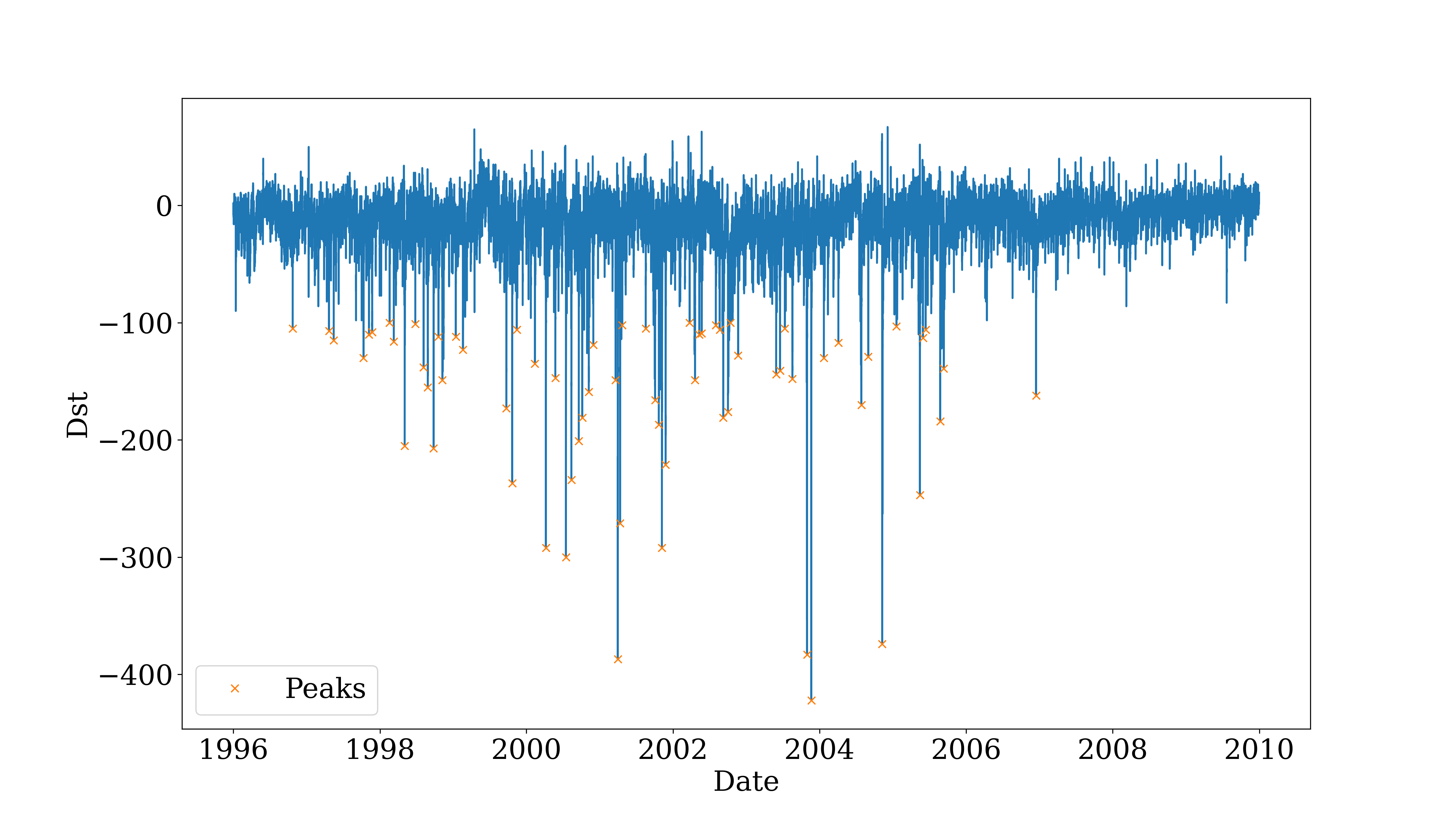
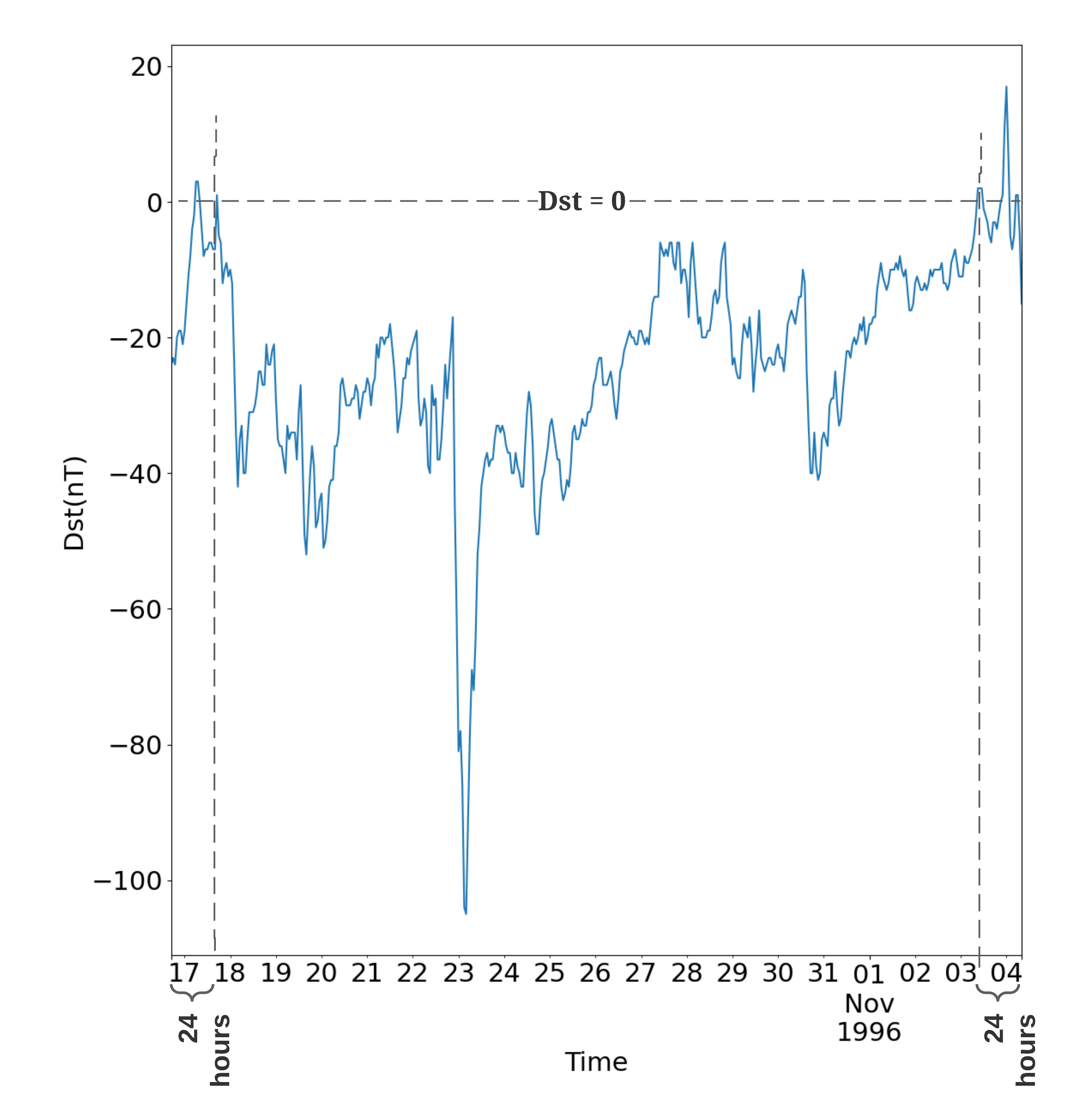
The index is available at 1-hour cadence from the NASA OMNI database. Fig. 1 displays the index in the period 1996-2010. The model is trained, validated and tested on storm events with a peak smaller than -100 nT, shown by orange crosses. Overall, 51 such storm periods are selected for this study. In order to define a storm period, we look for the the nearest positive values immediately before and after each peak, and then extend the time window by a 24-hour buffer zone to make sure that the pre-storm period and the recovery phase are fully included. An example is shown in Fig. 2, where the Dst peak is observed on Oct. 23, 1996. The storm period is defined as ranging between Oct. 17, 1996 and Nov. 04, 1996. With this procedure we make sure that the time intervals are selected in such a way that the negative peaks do not always occur at the same time within the chosen storm-time window, hence the neural network does not simply memorize. The average period of selected storm events is approximately 15 days. All selected storms, sorted by peak , are listed in Table. 1.
| No. | Start time | End time | Min. Dst (nT) |
|---|---|---|---|
| 1 | 2001-03-29 03:00:00 | 2001-04-06 15:00:00 | -387 |
| 2 | 2001-11-03 19:00:00 | 2001-11-17 00:00:00 | -292 |
| 3 | 2005-05-13 05:00:00 | 2005-05-22 04:00:00 | -247 |
| 4 | 1999-10-19 23:00:00 | 1999-11-02 11:00:00 | -237 |
| 5 | 2000-08-08 05:00:00 | 2000-08-21 07:00:00 | -234 |
| 6 | 2001-11-22 06:00:00 | 2001-12-02 14:00:00 | -221 |
| 7 | 2000-09-15 19:00:00 | 2000-09-26 14:00:00 | -201 |
| 8 | 2001-10-17 10:00:00 | 2001-10-27 09:00:00 | -187 |
| 9 | 2005-08-22 08:00:00 | 2005-09-02 03:00:00 | -184 |
| 10 | 2002-09-01 23:00:00 | 2002-09-18 07:00:00 | -181 |
| 11 | 1999-09-20 20:00:00 | 1999-09-28 15:00:00 | -173 |
| 12 | 2000-11-02 04:00:00 | 2000-11-12 06:00:00 | -159 |
| 13 | 2001-03-17 11:00:00 | 2001-03-24 14:00:00 | -149 |
| 14 | 2003-08-15 18:00:00 | 2003-09-02 23:00:00 | -148 |
| 15 | 2003-06-14 09:00:00 | 2003-06-28 12:00:00 | -141 |
| 16 | 2000-02-09 07:00:00 | 2000-02-21 12:00:00 | -135 |
| 17 | 2004-01-20 05:00:00 | 2004-02-01 05:00:00 | -130 |
| 18 | 2004-08-28 02:00:00 | 2004-09-06 01:00:00 | -129 |
| 19 | 2000-11-24 22:00:00 | 2000-12-05 05:00:00 | -119 |
| 20 | 2002-05-09 11:00:00 | 2002-05-20 20:00:00 | -110 |
| 21 | 2002-05-21 11:00:00 | 2002-06-01 20:00:00 | -109 |
| 22 | 2002-08-16 22:00:00 | 2002-08-27 10:00:00 | -106 |
| 23 | 2001-08-15 16:00:00 | 2001-08-21 12:00:00 | -105 |
| 24 | 2005-01-14 21:00:00 | 2005-01-23 17:00:00 | -103 |
| 25 | 2002-07-30 23:00:00 | 2002-08-09 03:00:00 | -102 |
| 26 | 2002-03-21 15:00:00 | 2002-03-30 21:00:00 | -100 |
| 27 | 2000-01-20 16:00:00 | 2000-01-29 06:00:00 | -96 |
| 28 | 2005-01-05 14:00:00 | 2005-01-13 18:00:00 | -93 |
| 29 | 2004-02-09 10:00:00 | 2004-02-23 20:00:00 | -93 |
| 30 | 1999-04-14 20:00:00 | 1999-04-23 08:00:00 | -91 |
| 31 | 2000-06-06 13:00:00 | 2000-06-15 01:00:00 | -90 |
| 32 | 2002-01-31 00:00:00 | 2002-02-06 21:00:00 | -86 |
| 33 | 1999-12-02 02:00:00 | 1999-12-17 07:00:00 | -85 |
| 34 | 2003-05-07 08:00:00 | 2003-05-20 06:00:00 | -84 |
| 35 | 2009-07-20 01:00:00 | 2009-08-01 10:00:00 | -83 |
| 36 | 2010-03-29 23:00:00 | 2010-04-16 16:00:00 | -81 |
| 37 | 2005-02-14 12:00:00 | 2005-02-24 09:00:00 | -80 |
| 38 | 2000-01-09 10:00:00 | 2000-01-19 11:00:00 | -80 |
| 39 | 2010-05-26 21:00:00 | 2010-06-10 15:00:00 | -80 |
| 40 | 2004-03-07 13:00:00 | 2004-03-21 21:00:00 | -78 |
| 41 | 2004-07-14 22:00:00 | 2004-07-22 18:00:00 | -76 |
| 42 | 2001-05-05 00:00:00 | 2001-05-18 18:00:00 | -76 |
| 43 | 2000-06-24 02:00:00 | 2000-07-02 09:00:00 | -75 |
| 44 | 2002-12-17 08:00:00 | 2002-12-24 16:00:00 | -75 |
| 45 | 2005-10-29 09:00:00 | 2005-11-04 18:00:00 | -74 |
| 46 | 2003-01-27 13:00:00 | 2003-02-15 13:00:00 | -74 |
| 47 | 2007-03-21 10:00:00 | 2007-03-27 00:00:00 | -72 |
| 48 | 2002-02-26 17:00:00 | 2002-03-05 01:00:00 | -71 |
| 49 | 2010-04-30 11:00:00 | 2010-05-12 17:00:00 | -71 |
| 50 | 1999-10-08 01:00:00 | 1999-10-22 04:00:00 | -67 |
| 51 | 2003-02-24 22:00:00 | 2003-03-14 15:00:00 | -67 |
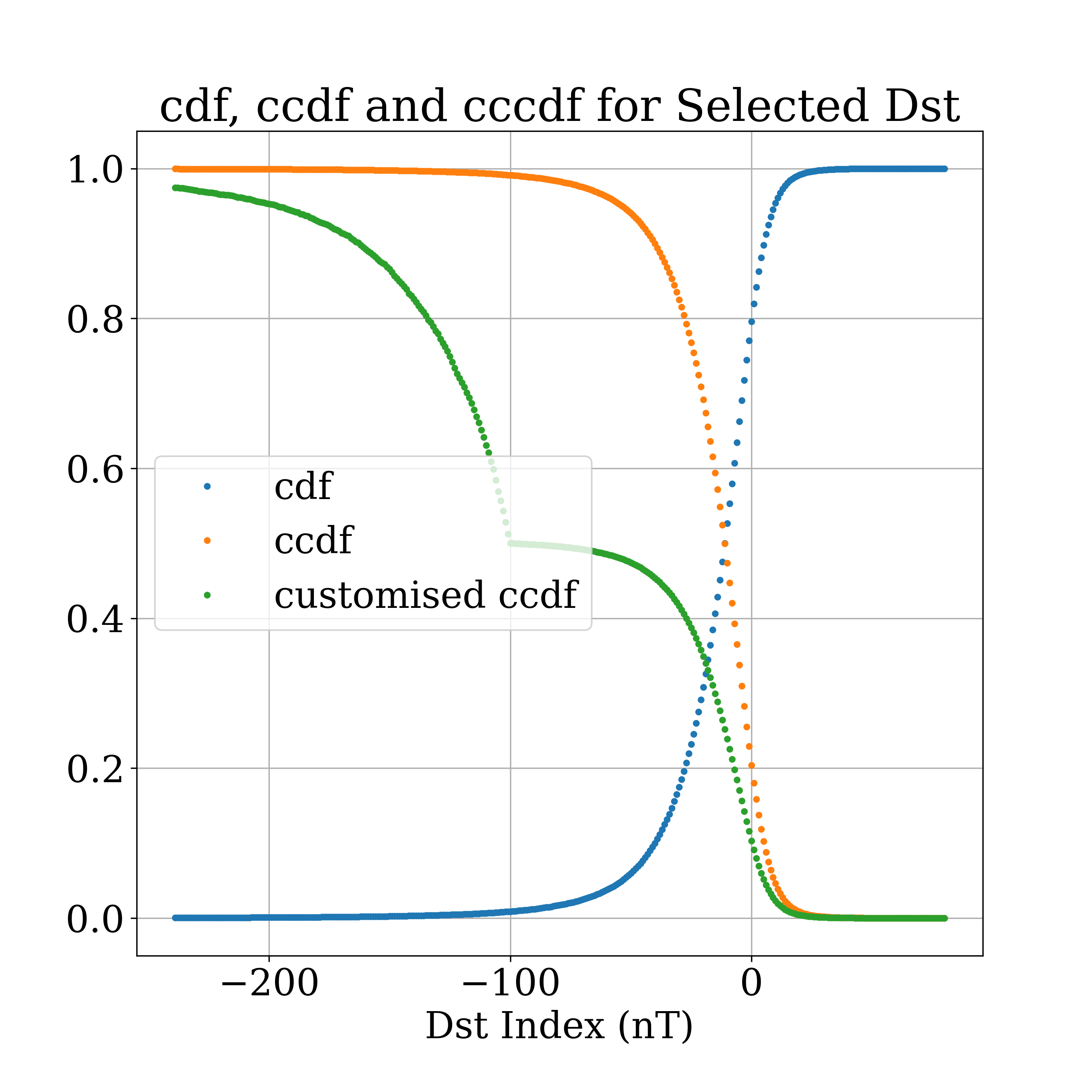
As mentioned in the Introduction, we would like to solve this classification task by a regression model. Hence, instead of a binary label set (positive/negative), a customized complementary cumulative probability distribution function (CCCDF) of is used as a target for the CNN model. The CCCDF is shown in Fig. 3, and explained briefly below. A cumulative distribution function (CDF) is defined as the integral of a probability density function (PDF) from negative infinity to and the complementary CDF (CCDF) = 1-CDF or the integral from positive infinity to . The CDF() is the probability that a random variable has a value less than . Conversely, the CCDF() gives the probability that the variable under consideration is larger than . The customized CCDF (CCCDF) for =-100nT is defined as in Eqn. 1-2. Note that CCCDF(=-100) =0.5 by construction.
| (1) |
| (2) |
2.2 SoHO mission
The two-hourly SoHO data sets used in this work for the period 1996-05-01 to 2011-04-12 are derived from the following public domain resources: the NASA Solar Data Analysis Center’s (SDAC) Virtual Solar Observatory (VSO) (https://sdac.virtualsolar.org/cgi/search) and Stanford University’s Joint Science Operation Center (JSOC) http://jsoc.stanford.edu/MDI/MDI_Magnetograms.html. All SoHO products and their details are shown in Table 2.
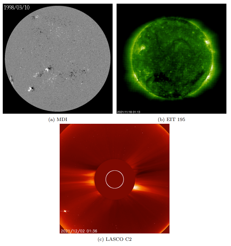
More than 20,000 SOHO images can be provided from three on-board instruments, including the Michelson Doppler Imager (MDI) for the solar photosphere, the Extreme ultraviolet Imaging Telescope (EIT) for the stellar atmosphere to low corona, and the Large Angle and Spectrometric Coronagraph (LASCO) covering the corona from . Those data have fully covered Solar Cycle and . Among them, MDI, EIT with a wavelength of 195 (EIT-195) and LASCO-C2 are used as the inputs of this study.
However, the SDAC data is highly heterogeneous. Not only are there intrinsic differences among these SoHO products (e.g., individual cadence for each channel shown in Table 2), but there is also an irregular assortment of image file sizes and processing levels. All products require calibration before they can be used for the neural networks. In addition, each channel needs to be synchronized with a fixed cadence (i.e., 2hrs in this study). An example of the calibrated data are shown in Fig. 4.
A pipeline has been created and published by [Shneider \BOthers. (\APACyear2021)] for automatically downloading, cleaning and synchronizing these original images from SDAC and VSO. A machine-learning-ready image data set is then provided which is a valuable resource for the space weather community.
| Instrument | Detector | Observed Region | Å | Cadence (min) | Date Range |
| MDI | MDI | Full Disk | (Ni I) | 1996.05.01 - 2011.04.12 | |
| EIT | EIT | Full Disk | (Fe IX/X) | 1996.01.01 | |
| EIT | EIT | Full Disk | (Fe XII) | 1996.01.01 | |
| EIT | EIT | Full Disk | (Fe XV) | 1996.01.01 | |
| EIT | EIT | Full Disk | (He II) | 1996.01.01 | |
| LASCO | C2 | Corona () | Visible | 1995.12.08 | |
| LASCO | C3 | Corona () | Visible | 1995.12.08 |
3 Methodology
The goal of this study is to estimate the probability 1 to 3 days ahead of the time when full-disk SoHO images are taken. For the sake of clarity we discuss here the algorithm for 1-day ahead prediction, with the understanding that all times are correspondingly shifted for 2 and 3 days ahead predictions.
3.1 Customized Class-Balanced Convolutional Neural Networks (CB-CNN)
Several machine learning approaches can be used for a probabilistic prediction task. We have compared naive Bayes, multi-layer perception and CNN. Among them, CNN has yielded the most reliable and robust performance (results are not shown here).
CNN is a commonly used neural network architecture, widely used in computer vision [Gu \BOthers. (\APACyear2018)], in solar image processing [Illarionov \BBA Tlatov (\APACyear2018), Baso \BBA Ramos (\APACyear2018), Upendran \BOthers. (\APACyear2020), Dos Santos \BOthers. (\APACyear2021)], and recently in plasma and space physics applications [Hu \BOthers. (\APACyear2020), Siciliano \BOthers. (\APACyear2021)]. Hence, in this study, we have opted to use a customized class-balanced convolutional neural network (CNN). This is because of the imbalance between the number of positive samples () and the number of negative samples (), which is approximately 10% of all training samples. As a result of using a class-balanced target, the CB-CNN model performs better than a vanilla CNN model, when the target is near the classification threshold. A brief introduction of the CNN architecture and the optimization methods used in the training is listed in Table 3.
| Parameter | Value |
|---|---|
| input size | [3, 256, 256] |
| output size | 12 |
| layers | 3 |
| kernel size | [3, 5, 5] |
| padding mode | same |
| activation function | [ReLU, ReLU, ReLU] |
| max epochs | 100 |
| optimization | AdamW |
| learning rate | 0.0001 |
| regularization | Elastic |
| cost function | CB-MSE |
By denoting with the time at which the input images are taken, a multi-target CNN model is first trained to predict the probability in the time range , with a time resolution of 2 hours. That is, 12 probability values are output for each input. This means that, at any given time, we have 12 probabilities that have been predicted between 26 and 48 hours ahead. Note that, due to the variability of the Sun and because we are using full disk images, predictions with shorter time lags are not necessarily more accurate than ones with longer time lags. Because we eventually want to merge those predictions (with different time lags) into a unique, reliable prediction, we do not use a standard loss function for binary classification (such as, e.g., binary cross-entropy), but a customized, class-balanced, mean square error.
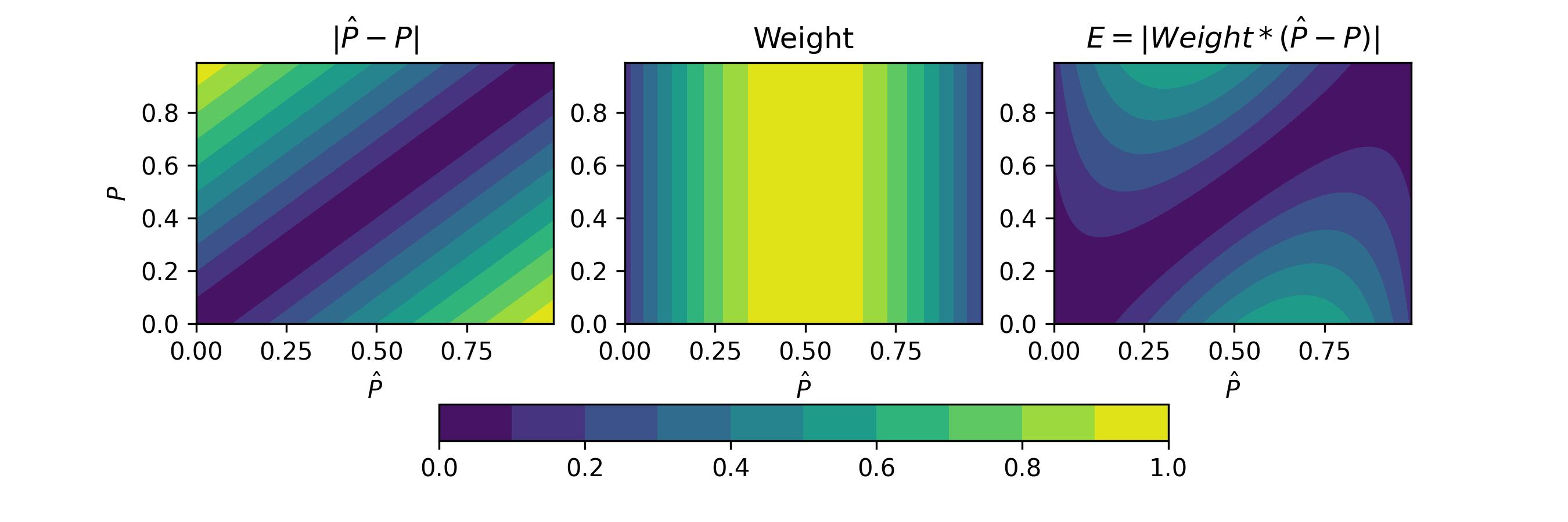
In our application, a class-balanced loss function developed by \citeAcui2019class is used to deal with the large imbalance between positive and negative labels. In addition to that, we want to penalize more the incorrect predictions that are closes to the decision boundary (corresponding to the threshold ). Hence, a customized weight is designed to artificially increase the cost function for the possibly ambiguous samples with near -100 nT. The cost function is defined as:
| (3) |
| (4) |
Where is the model prediction for th sample with a delay hour (delay hours ranging 26h, 28h, , 48h), is the corresponding target, and are the number of positive and negative samples in a batch, respectively, and denotes the weight associated to each target. The detailed procedure of optimizing these weights will be further introduced in Section 3.3. is a customized square error that penalizes samples whose is near -100 nT, as shown in Fig. 5. is a constant term manually set to 0.9999 according to \citeAcui2019class.
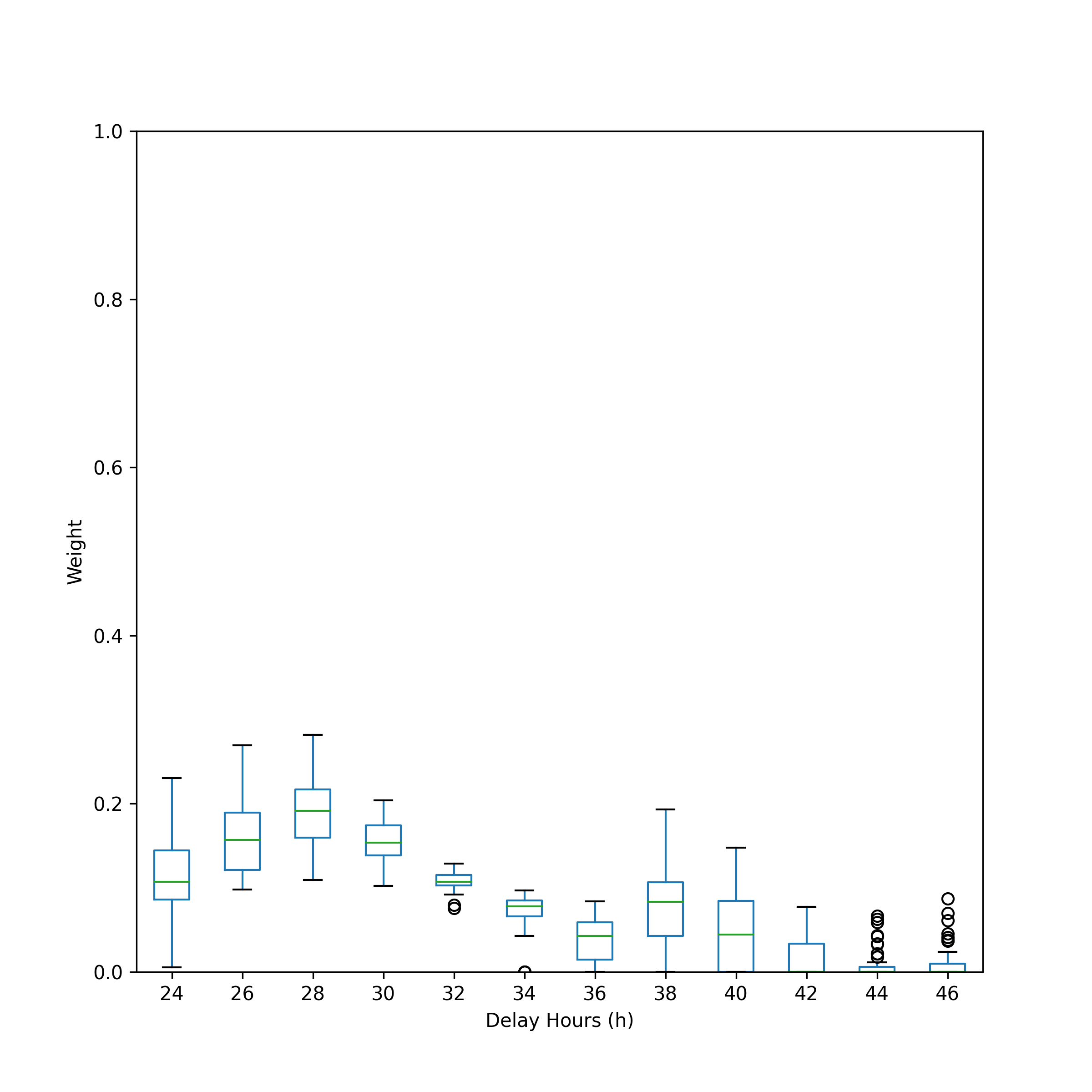
The multi-target CNN trained using the cost function described above, can then be used to forecast the Dst probability from 26 to 48 hours ahead, at a 2 hours rate. Hence, at any given time we have different predictions (issued between 26 and 48 hours prior). A natural question then arises on whether one could combine these 12 predictions in order to achieve a prediction that is more accurate than any individual one. In order to to that, we take a weighted average of the 12 predictions, and we estimate the optimal (static) weights by solving a least squares (LS) problem. The details of the weight estimate procedure are shown in Fig. 8. Figure 9 shows the learned 12 weights optimized with this procedure, along with their uncertainty (see the leave-one-out procedure described below).
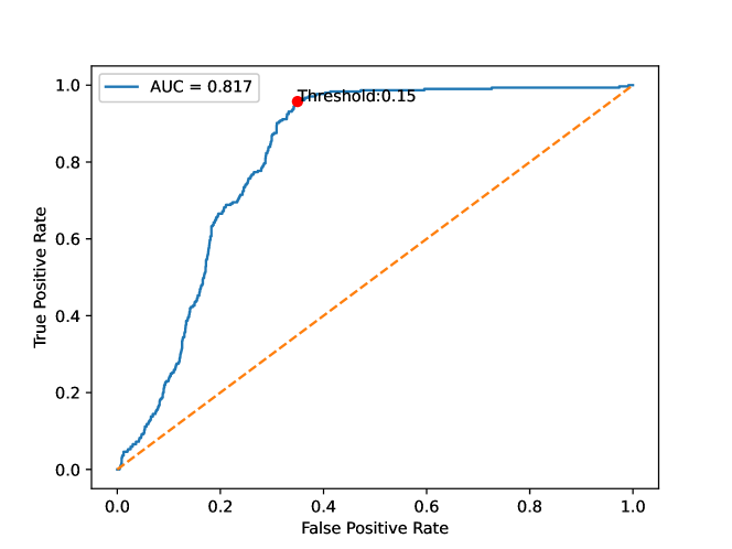
Finally, we notice that the predicted Dst probabilities might not be well-calibrated (i.e., statistically consistent with observations) and that the optimal threshold for binary classification metrics might be different than the standard 50% probability. Hence, the threshold of probability used for metrics (see Metrics Section) is re-calibrated by using a receiver operating characteristic (ROC) curve. ROC curve is an important diagnostic for a probabilistic model that can be used to determine an optimal threshold to separate positives from negatives based on probabilistic predictions. A detailed description of ROC curve can be found in \citeAcamporeale2020gray. An example ROC curve for the developed model with the CNN is shown in Fig. 6. Horizontal and vertical axes denote false positive rate (FPR) and true positive rate (TPR), respectively. The dashed orange line shows TPR equals to FPR (i.e., no skill), while the blue line represents the ROC curve, obtained by defining positives and negatives by progressively changing the probability threshold from 0% to 100%. The red dot represents the optimal/largest value of True Skill Statistics, defined as the difference (TPR-FPR).
3.2 Metrics
In order to precisely assess the accuracy of a model, it is important that the performance metrics are computed on a test set independent from the training set (so-called hold-out data), hence making sure that the machine learning algorithm does actually learn meaningful patterns and does not merely memorize the training data. A ‘Leave one out’ technique is adopted here. That is a K-fold cross validation taken to its logical extreme, with K equal to N, the number of selected storm cases. That means that the proposed model is trained on all the data except for one storm window and a prediction is made for that left-out storm. The procedure is repeated N times. Finally, the metrics are computed as averages over the N models. In this study, the top 51 storm windows in the period 1999-01-01 to 2011-04-10 constitute each a fold. Details of those events can be found in SI. The probabilistic predictions can be transformed to binary labels upon defining a probability threshold. In this way we can use standard metrics for binary classification such as the True Skill Statistic (TSS) and Matthews Correlation Coefficient (MCC)[Camporeale \BOthers. (\APACyear2020)]:
| TSS | (5) | |||
| (6) |
where TP, FP, TN and FN denotes true positive, false positive, true negative and false negative numbers respectively. The MCC score is a reliable statistical rate that produces a high score only if the prediction obtained good results in all of the four confusion matrix categories (TP, FP, TN and FN), proportionally both to the size of positive elements and the size of negative elements in the data set [Baldi \BOthers. (\APACyear2000)]. TSS is a useful metric that combines both types of information and should be as close as possible to 1. Those metrics have shown some advantages over the F1 score and accuracy in binary classification evaluation [Chicco \BBA Jurman (\APACyear2020)]. Moreover, an innovative way to evaluate the model accuracy has been developed by \citeAguastavino2021bad. This method assign different weights to FPs that anticipate the occurrence of an actual positive event (i.e. ’almost hit’). The value-weighted MCC and TSS have been proved more appropriate for decision making processes. Hence, these weighted scores are also considered to assess the model accuracy.
3.3 Ensemble Method
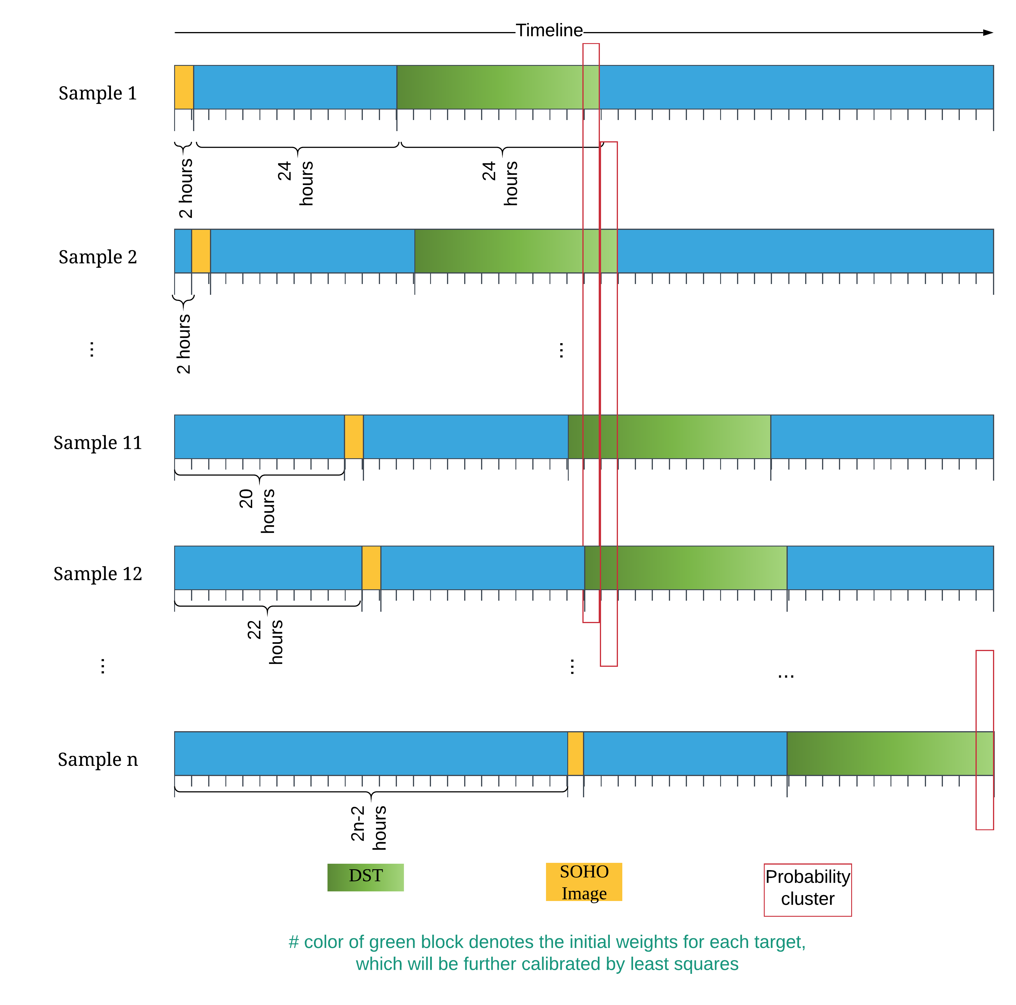
After the CNN model is developed, twelve probabilities can be predicted from the model and each SOHO image set. Although each prediction is per se valid, we have verified that combining those predictions yields a model that outperforms a single individual prediction. Here, we describe the ensemble method that, for simplicity, has been chosen to be a simple linear combination of the twelve probabilities so that the final probability is defined as , with the probability of Dst exceeding the -100 nT threshold at time . The timeline of predictions is depicted in Fig. 7. Each horizontal bar displays the timeline during an hypothetical event. Yellow blocks denote the 2 hours interval during which SoHO images are taken, and used as inputs to the model. The green block denotes the 12 probability predictions. From top to bottom, there are samples during one event. The time gap between consecutive samples is 2 hours. All predicted probabilities enclosed by a red frame are considered as one probability cluster (i.e., a vector) for a certain time epoch. The totality of clusters are used to form a design matrix for this event, i.e., a matrix. Assuming we have events, the whole design matrix has then size . Eqn. 7 is the observation model of the ensemble method:
| (7) |
where is the design matrix as introduced in Fig. 7 (each column of contains 12 different probabilities collected with different time lags):
| (8) |
denotes the ground truth (i.e., the CCCDF of ), and is the sought after weight vector. is initially set to a constant vector, and will be optimized by a least-square (LS) method:
| (9) |
In this study, we develop a customized Elastic-net-aided LS method to optimize the weights , based on the elastic-net regularization scheme proposed by Zou and Hastiea [Zou \BBA Hastie (\APACyear2005)]. The residuals are calculated as:
| (10) |
The cost function, or so-called normal function in LS, is defined as:
| (11) |
The first term in is a classic weighted cost function where is the transpose matrix of V. The second and third terms are Elastic net regularization factors that linearly combines the L1 and L2 penalties of the lasso and ridge methods. Based on the experiments on the storms, here we set , and . Finally, denotes the ‘weight’, i.e., diagonal matrix with positive and negative samples as defined in Eqn. 12.
| (12) |
The function reaches a minimum when the partial derivative of with respect to equals zero:
| (13) |
where is a vector and is a unit vector times scale .
or
| (14) |
Multiplying with Eqn. 10, one has
| (15) |
| (16) |
Finally,
| (17) |
4 Results
In this section we show the results of our model in terms of the metrics TSS and MCC scores discussed in Section 3.2. It should be noted that, by using the leave-one-out technique, all metrics in this section are calculated based on the combination of all entries in the confusion matrix. The proposed ensemble approach is compared against three alternative approaches: support vector regression (SVR) which is a non-linear ensemble method [Awad \BBA Khanna (\APACyear2015)], a method where ensemble members are simply averaged (equal weight, denoted as ‘Constant’ in Table 4), and a single individual prediction 24 hrs ahead (no ensemble, so-called ‘Single’ in Table 4). Table 4 shows the TSS and MCC for the four methods. One can notice that the LS ensemble method significantly outperforms the single individual prediction model. Moreover, although SVR yields a large TNR, the FPR is also large, resulting in low values for both TSS and MCC.
| Ensemble Method | TSS | MCC | TP | FP | TN | FN |
|---|---|---|---|---|---|---|
| LS | 0.62 | 0.37 | 57 | 209 | 1738 | 21 |
| SVR | 0.15 | 0.18 | 13 | 37 | 1910 | 65 |
| Constant | 0.32 | 0.23 | 31 | 135 | 1812 | 47 |
| Single | 0.28 | 0.17 | 103 | 544 | 2097 | 111 |
As anticipated in Section 1, the goal of this work is not just to provide a binary classification, but rather to estimate the probability of exceeding predefined thresholds. The LS-ensemble method has been trained and tested for various thresholds (Table 5), different forecast duration (see Table 6) and larger time resolution (Table 7). Table 5 demonstrates that the model performs best when the threshold is -100 nT. Corresponding TSS and MCC are 0.62 and 0.37, respectively. Both TSS and MCC decrease when the threshold is set to -50 nT. Although TSS performs well with a threshold of -200 nT, the corresponding MCC decreases significantly because of the imbalanced labels since very few ‘very strong’ storms ( -200 nT) occurred during 1999-2009. This implies that the proposed method may identify strong storms ( -100 nT) better than mild storms ( -50 nT). Table 6 shows how the performance of the model gets worse with a longer lead-time. From Table 7, we can see that the model trained from 2-hrs samples outperforms the model trained from 6-hrs samples. This is because a 6-hrs samples traninig set is composed of fewer samples overall. Therefore, the model could be less robust with a larger cadence. Finally, we show in Table 8 the modified TSS and MCC scores proposed in \citeAguastavino2021bad that further improve the accuracy of the method.
A statistic analysis of weights from all of the 51 sub-models is plotted in Fig. 9. Green horizontal lines denote the mean weights from all 51 sub-models. Blue bars represent the uncertainty range between the first and the third quartile of the distributions, and black dots are distribution outliers. Fig. 9 shows that the predictions at 24-38 delay hours have the largest contributions to the final probability. The weights decrease with the increase of delay hours. It is interesting that the contribution of predictions during 42 to 46 delay hours are essentially negligible. The error bars and presence of outliers also imply that the weights vary slightly according to different storms. This may be improved by having more representative storm events.
| threshold | TSS | MCC | TP | FP | TN | FN |
|---|---|---|---|---|---|---|
| -50 nT | 0.29 | 0.26 | 215 | 350 | 1254 | 206 |
| -100 nT | 0.62 | 0.37 | 57 | 209 | 1738 | 21 |
| -200 nT | 0.56 | 0.14 | 3 | 80 | 1940 | 2 |
| Forecast (Days) | TSS | MCC | TP | FP | TN | FN |
|---|---|---|---|---|---|---|
| 1 | 0.62 | 0.37 | 57 | 209 | 1738 | 21 |
| 2 | 0.34 | 0.30 | 40 | 93 | 1807 | 63 |
| 3 | 0.27 | 0.17 | 44 | 248 | 1578 | 65 |
| time resolution | TSS | MCC | TP | FP | TN | FN |
|---|---|---|---|---|---|---|
| 2 | 0.62 | 0.37 | 57 | 209 | 1738 | 21 |
| 6 | 0.42 | 0.25 | 9 | 47 | 555 | 9 |
| time res | wTSS | wMCC | wTP | wFP | wTN | wFN |
|---|---|---|---|---|---|---|
| 2 | 0.68 | 0.47 | 67 | 133 | 1407 | 20 |
| 6 | 0.59 | 0.42 | 41 | 82 | 510 | 15 |
4.1 Storm Case Study
In this section we would like to investigate several typical storm cases.
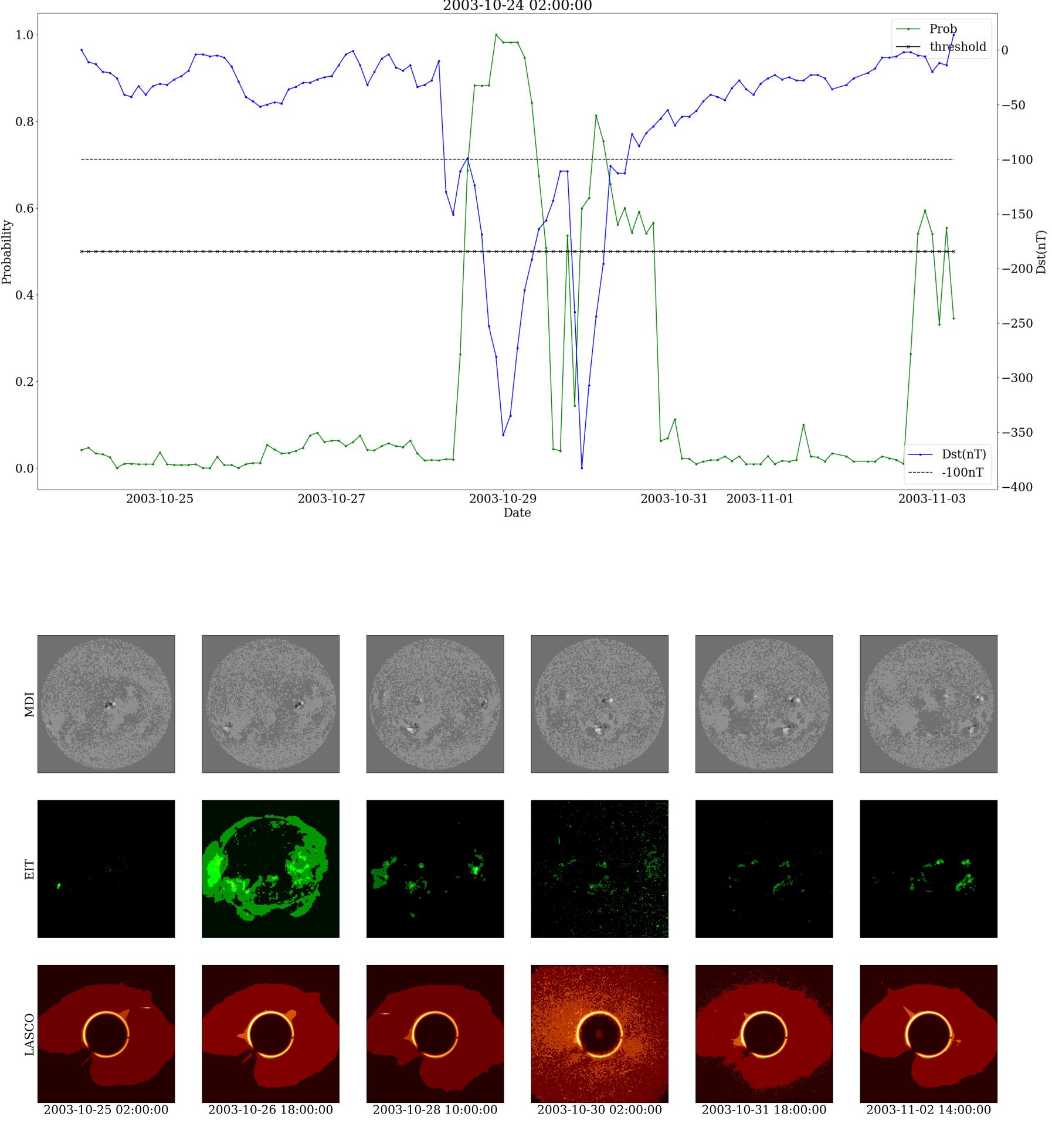
The Halloween storm, caused by a CME, from 2003-10-25 to 2003-11-05 is selected for a case study. This is the biggest storm in the past 20 years. Figure 10 displays the 24-hour ahead probabilities of the developed model (green line, left vertical axis) and the corresponding (blue line, right vertical axis) during the Halloween storm. Black cross and dotted lines are the threshold of probability and index, respectively.
The predicted probabilities can be converted to a binary format with an optimal threshold re-calibrated by training samples. This threshold is rescaled back to 0.5 in Fig. 10. Two peaks at the midnight October 29 & 30 can be well captured by these predicted probabilities. The time shift between the peak of real and the peak of the predicted probability is no more than 4 hours. This implies that those strong storm can predicted very well by the proposed model.
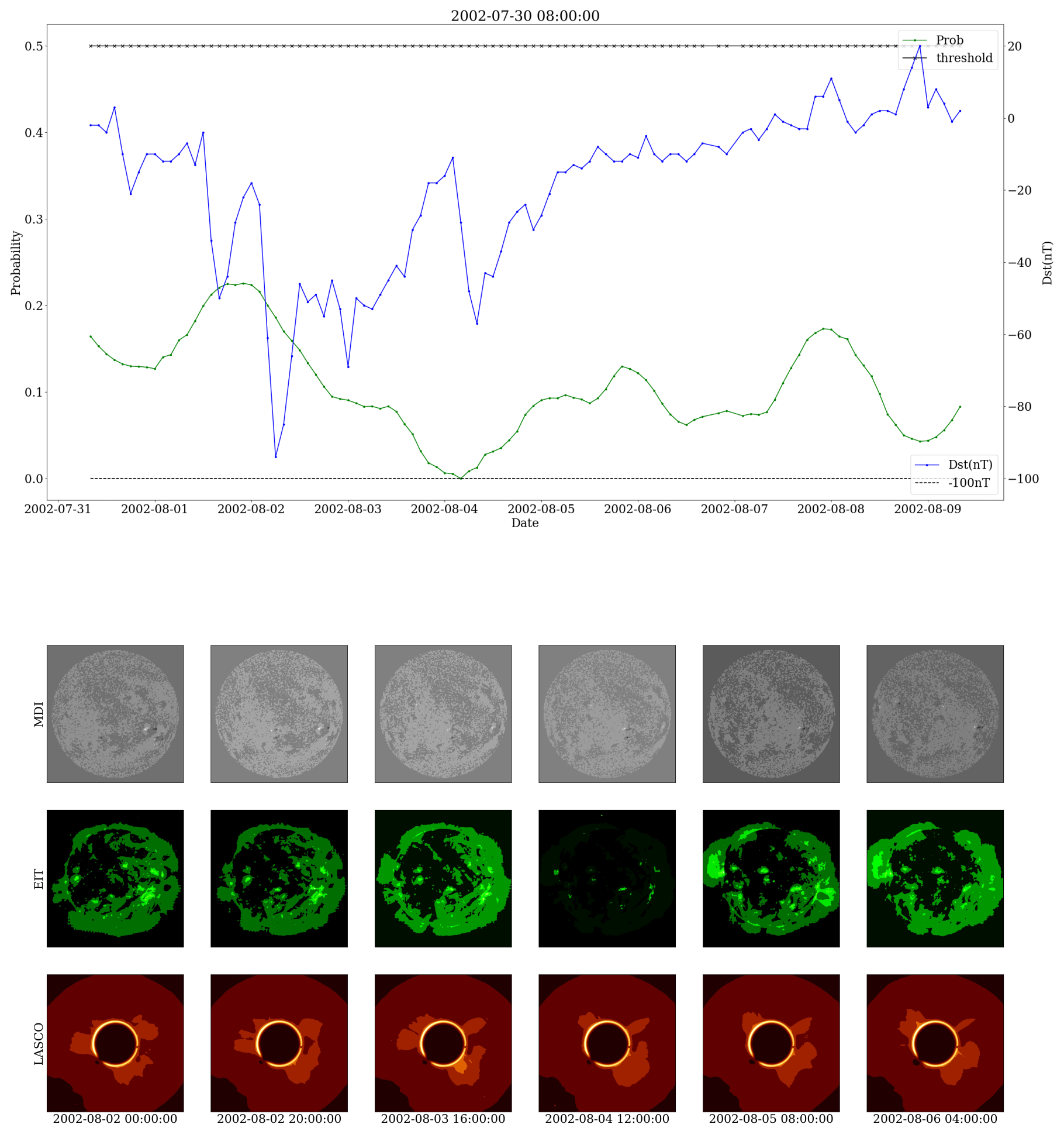
Fig. 10 also indicates that the proposed model can forecast well those storms caused by CME because they stand out very clearly in SoHO images. However, a good portion of solar CMEs are non-Earth oriented. The ability of this model to identify the geo-effectivenes (or lack thereof) of non-Earth-directed CMEs is also assessed. Twenty of them occurring in the period 2000-2003 are selected for validation. The TSS and MCC of the prediction based on the developed model during those non-Earth-directed CME periods are 0.94 and 0.46 respectively. The TP, FP, TN and FN values are 14, 50, 709 and 0. An example is shown in Fig. 11. A strong CME occurred around 2002-07-30, but the corresponding did not reach -100 nT. The predicted probability increases but not as significantly as for the Earth-directed CMEs. This suggests that the proposed model may be able to distinguish non-Earth-directed CMEs, and assign lower probabilities to them. Similar plots of probabilities for all the other storm events used in this study are included as supplementary information.
5 Summary & Outlook
We have developed a LS-based class-balanced ensemble CNN model that estimates the probability of exceeding a given threshold 1 day ahead based on SoHO images. 51 selected storm events were chosen during a long‐span historical data set ( 16 years), between 1996-05-01 and 2011-04-20. The proposed model can predict the probability that nT 24 hours ahead with a TSS of 0.62 and MCC of 0.37. The weighted TSS and MCC from \citeAguastavino2021bad are 0.68 and 0.47.
One of the crucial points of this work is that it combines a LS ensemble method with a CNN algorithm for a probability prediction. A customized class-balanced mean square error is developed as the cost function of the proposed CNN model. After the CNN model is developed, a LS method is developed to estimate the weights of the predictions from the proposed multi-target CNNs. Eventually a final probability value can be calculated by the optimized weights and CNN predictions. Binary classification of each event is then determined by a threshold re-calibrated on the other 50 storms used for training.
We have shown that this proposed model provides good skills for predicting 1-day-ahead during strong storm periods. The proposed model can also forecast probability even within a non-Earth-direct CME period. This model will extend the prediction lead time of most of the current empirical prediction models. The performance metrics that we have analyzed are the confusion matrix, TSS, MCC, and corresponding weighted scores from [Guastavino \BOthers. (\APACyear2021)]. Finally, we have discussed a strong storm case from 2003-10-25 to 2003-11-05. peaks can be well captured by the developed model.
A possible weakness of this model is that the weights are static, although the time lags from different events should not be the same [Chandorkar \BOthers. (\APACyear2019)]. As a next step, we plan to take into account dynamic weights, e.g. by applying an online/dynamic ensemble method, such as [Monteleoni \BOthers. (\APACyear2011)]. Moreover, storms that result from CMEs or high speed streamers are based on different physical mechanisms. The former mostly occur during high solar activity period, while the latter are seen more often during low solar activity period. Including a solar activity index, such as into consideration to first classify those samples in order to train the model more precisely, will be also experimented in the future.
Acknowledgements.
This project has been developed in the framework of the European project AIDA. The AIDA project has received funding from the European Union’s Horizon 2020 Research and Innovation programme under grant agreement No 776262. EC is partially funded by the National Aeronautics and Space Administration under grants 80NSSC20K1580, 80NSSC20K1275, 80NSSC21K1555. We thank OMNIWeb for providing the data (https://omniweb.gsfc.nasa.gov/), the NASA Solar Data Analysis Center’s (SDAC) Virtual Solar Observatory (VSO) (https://sdac.virtualsolar.org/cgi/search) and Stanford University’s Joint Science Operation Center (JSOC) http://jsoc.stanford.edu/MDI/MDI_Magnetograms.html for SoHO images. All the results and codes have been made available as a Zenodo repository in 10.5281/zenodo.6385325. Future updates can be found on https://github.com/HuanWinter/Dst_SoHO and https://ml-space-weather.github.io/projects.html (under construction)References
- Awad \BBA Khanna (\APACyear2015) \APACinsertmetastarawad2015support{APACrefauthors}Awad, M.\BCBT \BBA Khanna, R. \APACrefYearMonthDay2015. \BBOQ\APACrefatitleSupport vector regression Support vector regression.\BBCQ \BIn \APACrefbtitleEfficient learning machines Efficient learning machines (\BPGS 67–80). \APACaddressPublisherSpringer. \PrintBackRefs\CurrentBib
- Bala \BBA Reiff (\APACyear2012) \APACinsertmetastarbala2012improvements{APACrefauthors}Bala, R.\BCBT \BBA Reiff, P. \APACrefYearMonthDay2012. \BBOQ\APACrefatitleImprovements in short-term forecasting of geomagnetic activity Improvements in short-term forecasting of geomagnetic activity.\BBCQ \APACjournalVolNumPagesSpace Weather106. \PrintBackRefs\CurrentBib
- Baldi \BOthers. (\APACyear2000) \APACinsertmetastarbaldi2000assessing{APACrefauthors}Baldi, P., Brunak, S., Chauvin, Y., Andersen, C\BPBIA.\BCBL \BBA Nielsen, H. \APACrefYearMonthDay2000. \BBOQ\APACrefatitleAssessing the accuracy of prediction algorithms for classification: an overview Assessing the accuracy of prediction algorithms for classification: an overview.\BBCQ \APACjournalVolNumPagesBioinformatics165412–424. \PrintBackRefs\CurrentBib
- Baso \BBA Ramos (\APACyear2018) \APACinsertmetastarbaso2018enhancing{APACrefauthors}Baso, C\BPBID.\BCBT \BBA Ramos, A\BPBIA. \APACrefYearMonthDay2018. \BBOQ\APACrefatitleEnhancing SDO/HMI images using deep learning Enhancing sdo/hmi images using deep learning.\BBCQ \APACjournalVolNumPagesAstronomy & Astrophysics614A5. \PrintBackRefs\CurrentBib
- Borovsky \BBA Shprits (\APACyear2017) \APACinsertmetastarborovsky2017dst{APACrefauthors}Borovsky, J\BPBIE.\BCBT \BBA Shprits, Y\BPBIY. \APACrefYearMonthDay2017. \BBOQ\APACrefatitleIs the Dst index sufficient to define all geospace storms? Is the dst index sufficient to define all geospace storms?\BBCQ \APACjournalVolNumPagesJournal of Geophysical Research: Space Physics1221111–543. \PrintBackRefs\CurrentBib
- Bowman \BOthers. (\APACyear2008) \APACinsertmetastarbowman2008new{APACrefauthors}Bowman, B., Tobiska, W\BPBIK., Marcos, F., Huang, C., Lin, C.\BCBL \BBA Burke, W. \APACrefYearMonthDay2008. \BBOQ\APACrefatitleA new empirical thermospheric density model JB2008 using new solar and geomagnetic indices A new empirical thermospheric density model jb2008 using new solar and geomagnetic indices.\BBCQ \BIn \APACrefbtitleAIAA/AAS astrodynamics specialist conference and exhibit Aiaa/aas astrodynamics specialist conference and exhibit (\BPG 6438). \PrintBackRefs\CurrentBib
- Brueckner \BOthers. (\APACyear1995) \APACinsertmetastarSoHO_lasco{APACrefauthors}Brueckner, G\BPBIE., Howard, R\BPBIA., Koomen, M\BPBIJ., Korendyke, C\BPBIM., Michels, D\BPBIJ., Moses, J\BPBID.\BDBLEyles, C\BPBIJ. \APACrefYearMonthDay1995\APACmonth12. \BBOQ\APACrefatitleThe Large Angle Spectroscopic Coronagraph (LASCO) The Large Angle Spectroscopic Coronagraph (LASCO).\BBCQ \APACjournalVolNumPagesSolar Physics1621-2357-402. {APACrefDOI} 10.1007/BF00733434 \PrintBackRefs\CurrentBib
- Camporeale (\APACyear2019) \APACinsertmetastarcamporeale2019challenge{APACrefauthors}Camporeale, E. \APACrefYearMonthDay2019. \BBOQ\APACrefatitleThe challenge of machine learning in space weather: Nowcasting and forecasting The challenge of machine learning in space weather: Nowcasting and forecasting.\BBCQ \APACjournalVolNumPagesSpace Weather1781166–1207. \PrintBackRefs\CurrentBib
- Camporeale \BOthers. (\APACyear2020) \APACinsertmetastarcamporeale2020gray{APACrefauthors}Camporeale, E., Cash, M\BPBID., Singer, H\BPBIJ., Balch, C\BPBIC., Huang, Z.\BCBL \BBA Toth, G. \APACrefYearMonthDay2020. \BBOQ\APACrefatitleA gray-box model for a probabilistic estimate of regional ground magnetic perturbations: Enhancing the NOAA operational Geospace model with machine learning A gray-box model for a probabilistic estimate of regional ground magnetic perturbations: Enhancing the noaa operational geospace model with machine learning.\BBCQ \APACjournalVolNumPagesJournal of Geophysical Research: Space Physics12511e2019JA027684. \PrintBackRefs\CurrentBib
- Chandorkar \BBA Camporeale (\APACyear2018) \APACinsertmetastarchandorkar2018probabilistic{APACrefauthors}Chandorkar, M.\BCBT \BBA Camporeale, E. \APACrefYearMonthDay2018. \BBOQ\APACrefatitleProbabilistic forecasting of geomagnetic indices using Gaussian process models Probabilistic forecasting of geomagnetic indices using gaussian process models.\BBCQ \BIn \APACrefbtitleMachine learning techniques for space weather Machine learning techniques for space weather (\BPGS 237–258). \APACaddressPublisherElsevier. \PrintBackRefs\CurrentBib
- Chandorkar \BOthers. (\APACyear2017) \APACinsertmetastarchandorkar2017probabilistic{APACrefauthors}Chandorkar, M., Camporeale, E.\BCBL \BBA Wing, S. \APACrefYearMonthDay2017. \BBOQ\APACrefatitleProbabilistic forecasting of the disturbance storm time index: An autoregressive Gaussian process approach Probabilistic forecasting of the disturbance storm time index: An autoregressive gaussian process approach.\BBCQ \APACjournalVolNumPagesSpace Weather1581004–1019. \PrintBackRefs\CurrentBib
- Chandorkar \BOthers. (\APACyear2019) \APACinsertmetastarchandorkar2019dynamic{APACrefauthors}Chandorkar, M., Furtlehner, C., Poduval, B., Camporeale, E.\BCBL \BBA Sebag, M. \APACrefYearMonthDay2019. \BBOQ\APACrefatitleDynamic time lag regression: predicting what & when Dynamic time lag regression: predicting what & when.\BBCQ \BIn \APACrefbtitleInternational Conference on Learning Representations. International conference on learning representations. \PrintBackRefs\CurrentBib
- Chicco \BBA Jurman (\APACyear2020) \APACinsertmetastarchicco2020advantages{APACrefauthors}Chicco, D.\BCBT \BBA Jurman, G. \APACrefYearMonthDay2020. \BBOQ\APACrefatitleThe advantages of the Matthews correlation coefficient (MCC) over F1 score and accuracy in binary classification evaluation The advantages of the matthews correlation coefficient (mcc) over f1 score and accuracy in binary classification evaluation.\BBCQ \APACjournalVolNumPagesBMC genomics2111–13. \PrintBackRefs\CurrentBib
- Cui \BOthers. (\APACyear2019) \APACinsertmetastarcui2019class{APACrefauthors}Cui, Y., Jia, M., Lin, T\BHBIY., Song, Y.\BCBL \BBA Belongie, S. \APACrefYearMonthDay2019. \BBOQ\APACrefatitleClass-balanced loss based on effective number of samples Class-balanced loss based on effective number of samples.\BBCQ \BIn \APACrefbtitleProceedings of the IEEE/CVF conference on computer vision and pattern recognition Proceedings of the ieee/cvf conference on computer vision and pattern recognition (\BPGS 9268–9277). \PrintBackRefs\CurrentBib
- Delaboudinière \BOthers. (\APACyear1995) \APACinsertmetastarSoHO_eit{APACrefauthors}Delaboudinière, J\BPBIP., Artzner, G\BPBIE., Brunaud, J., Gabriel, A\BPBIH., Hochedez, J\BPBIF., Millier, F.\BDBLvan Dessel, E\BPBIL. \APACrefYearMonthDay1995\APACmonth12. \BBOQ\APACrefatitleEIT: Extreme-Ultraviolet Imaging Telescope for the SOHO Mission EIT: Extreme-Ultraviolet Imaging Telescope for the SOHO Mission.\BBCQ \APACjournalVolNumPagesSolar Physics1621-2291-312. {APACrefDOI} 10.1007/BF00733432 \PrintBackRefs\CurrentBib
- Domingo \BOthers. (\APACyear1995) \APACinsertmetastarSoHO_overview{APACrefauthors}Domingo, V., Fleck, B.\BCBL \BBA Poland, A\BPBII. \APACrefYearMonthDay1995Dec. \BBOQ\APACrefatitleThe SOHO Mission: an Overview The SOHO Mission: an Overview.\BBCQ \APACjournalVolNumPagesSolar Physics1621-21-37. {APACrefDOI} 10.1007/BF00733425 \PrintBackRefs\CurrentBib
- Dos Santos \BOthers. (\APACyear2021) \APACinsertmetastardos2021multichannel{APACrefauthors}Dos Santos, L\BPBIF., Bose, S., Salvatelli, V., Neuberg, B., Cheung, M\BPBIC., Janvier, M.\BDBLBaydin, A\BPBIG. \APACrefYearMonthDay2021. \BBOQ\APACrefatitleMultichannel autocalibration for the Atmospheric Imaging Assembly using machine learning Multichannel autocalibration for the atmospheric imaging assembly using machine learning.\BBCQ \APACjournalVolNumPagesAstronomy & Astrophysics648A53. \PrintBackRefs\CurrentBib
- Gruet \BOthers. (\APACyear2018) \APACinsertmetastargruet2018multiple{APACrefauthors}Gruet, M\BPBIA., Chandorkar, M., Sicard, A.\BCBL \BBA Camporeale, E. \APACrefYearMonthDay2018. \BBOQ\APACrefatitleMultiple-Hour-Ahead Forecast of the Dst Index Using a Combination of Long Short-Term Memory Neural Network and Gaussian Process Multiple-hour-ahead forecast of the dst index using a combination of long short-term memory neural network and gaussian process.\BBCQ \APACjournalVolNumPagesSpace Weather16111882–1896. \PrintBackRefs\CurrentBib
- Gu \BOthers. (\APACyear2018) \APACinsertmetastargu2018recent{APACrefauthors}Gu, J., Wang, Z., Kuen, J., Ma, L., Shahroudy, A., Shuai, B.\BDBLothers \APACrefYearMonthDay2018. \BBOQ\APACrefatitleRecent advances in convolutional neural networks Recent advances in convolutional neural networks.\BBCQ \APACjournalVolNumPagesPattern Recognition77354–377. \PrintBackRefs\CurrentBib
- Guastavino \BOthers. (\APACyear2021) \APACinsertmetastarguastavino2021bad{APACrefauthors}Guastavino, S., Piana, M.\BCBL \BBA Benvenuto, F. \APACrefYearMonthDay2021. \BBOQ\APACrefatitleBad and good errors: value-weighted skill scores in deep ensemble learning Bad and good errors: value-weighted skill scores in deep ensemble learning.\BBCQ \APACjournalVolNumPagesarXiv preprint arXiv:2103.02881. \PrintBackRefs\CurrentBib
- Hu \BOthers. (\APACyear2020) \APACinsertmetastarhu2020identifying{APACrefauthors}Hu, A., Sisti, M., Finelli, F., Califano, F., Dargent, J., Faganello, M.\BDBLTeunissen, J. \APACrefYearMonthDay2020. \BBOQ\APACrefatitleIdentifying Magnetic Reconnection in 2D Hybrid Vlasov Maxwell Simulations with Convolutional Neural Networks Identifying magnetic reconnection in 2d hybrid vlasov maxwell simulations with convolutional neural networks.\BBCQ \APACjournalVolNumPagesThe Astrophysical Journal900186. \PrintBackRefs\CurrentBib
- Illarionov \BBA Tlatov (\APACyear2018) \APACinsertmetastarillarionov2018segmentation{APACrefauthors}Illarionov, E\BPBIA.\BCBT \BBA Tlatov, A\BPBIG. \APACrefYearMonthDay2018. \BBOQ\APACrefatitleSegmentation of coronal holes in solar disc images with a convolutional neural network Segmentation of coronal holes in solar disc images with a convolutional neural network.\BBCQ \APACjournalVolNumPagesMonthly Notices of the Royal Astronomical Society48145014–5021. \PrintBackRefs\CurrentBib
- Laperre \BOthers. (\APACyear2020) \APACinsertmetastarlaperre2020dynamic{APACrefauthors}Laperre, B., Amaya, J.\BCBL \BBA Lapenta, G. \APACrefYearMonthDay2020. \BBOQ\APACrefatitleDynamic Time Warping as a New Evaluation for Dst Forecast with Machine Learning Dynamic time warping as a new evaluation for dst forecast with machine learning.\BBCQ \APACjournalVolNumPagesarXiv preprint arXiv:2006.04667. \PrintBackRefs\CurrentBib
- Lazzús \BOthers. (\APACyear2017) \APACinsertmetastarlazzus2017forecasting{APACrefauthors}Lazzús, J., Vega, P., Rojas, P.\BCBL \BBA Salfate, I. \APACrefYearMonthDay2017. \BBOQ\APACrefatitleForecasting the Dst index using a swarm-optimized neural network Forecasting the dst index using a swarm-optimized neural network.\BBCQ \APACjournalVolNumPagesSpace Weather1581068–1089. \PrintBackRefs\CurrentBib
- Li \BOthers. (\APACyear2020) \APACinsertmetastarli2020predicting{APACrefauthors}Li, X., Zheng, Y., Wang, X.\BCBL \BBA Wang, L. \APACrefYearMonthDay2020. \BBOQ\APACrefatitlePredicting solar flares using a novel deep convolutional neural network Predicting solar flares using a novel deep convolutional neural network.\BBCQ \APACjournalVolNumPagesThe Astrophysical Journal891110. \PrintBackRefs\CurrentBib
- Licata \BOthers. (\APACyear2020) \APACinsertmetastarlicata2020benchmarking{APACrefauthors}Licata, R\BPBIJ., Tobiska, W\BPBIK.\BCBL \BBA Mehta, P\BPBIM. \APACrefYearMonthDay2020. \BBOQ\APACrefatitleBenchmarking forecasting models for space weather drivers Benchmarking forecasting models for space weather drivers.\BBCQ \APACjournalVolNumPagesSpace Weather1810e2020SW002496. \PrintBackRefs\CurrentBib
- Liemohn \BOthers. (\APACyear2001) \APACinsertmetastarliemohn2001dominant{APACrefauthors}Liemohn, M\BPBIW., Kozyra, J., Thomsen, M., Roeder, J., Lu, G., Borovsky, J.\BCBL \BBA Cayton, T. \APACrefYearMonthDay2001. \BBOQ\APACrefatitleDominant role of the asymmetric ring current in producing the stormtime Dst Dominant role of the asymmetric ring current in producing the stormtime dst.\BBCQ \APACjournalVolNumPagesJournal of Geophysical Research: Space Physics106A610883–10904. \PrintBackRefs\CurrentBib
- Lundstedt \BOthers. (\APACyear2002) \APACinsertmetastarlundstedt2002operational{APACrefauthors}Lundstedt, H., Gleisner, H.\BCBL \BBA Wintoft, P. \APACrefYearMonthDay2002. \BBOQ\APACrefatitleOperational forecasts of the geomagnetic Dst index Operational forecasts of the geomagnetic dst index.\BBCQ \APACjournalVolNumPagesGeophysical Research Letters292434–1. \PrintBackRefs\CurrentBib
- Monteleoni \BOthers. (\APACyear2011) \APACinsertmetastarmonteleoni2011tracking{APACrefauthors}Monteleoni, C., Schmidt, G\BPBIA., Saroha, S.\BCBL \BBA Asplund, E. \APACrefYearMonthDay2011. \BBOQ\APACrefatitleTracking climate models Tracking climate models.\BBCQ \APACjournalVolNumPagesStatistical Analysis and Data Mining: The ASA Data Science Journal44372–392. \PrintBackRefs\CurrentBib
- Park \BOthers. (\APACyear2018) \APACinsertmetastarpark2018application{APACrefauthors}Park, E., Moon, Y\BHBIJ., Shin, S., Yi, K., Lim, D., Lee, H.\BCBL \BBA Shin, G. \APACrefYearMonthDay2018. \BBOQ\APACrefatitleApplication of the deep convolutional neural network to the forecast of solar flare occurrence using full-disk solar magnetograms Application of the deep convolutional neural network to the forecast of solar flare occurrence using full-disk solar magnetograms.\BBCQ \APACjournalVolNumPagesThe Astrophysical Journal869291. \PrintBackRefs\CurrentBib
- Polikar (\APACyear2012) \APACinsertmetastarpolikar2012ensemble{APACrefauthors}Polikar, R. \APACrefYearMonthDay2012. \BBOQ\APACrefatitleEnsemble learning Ensemble learning.\BBCQ \BIn \APACrefbtitleEnsemble machine learning Ensemble machine learning (\BPGS 1–34). \APACaddressPublisherSpringer. \PrintBackRefs\CurrentBib
- Rostoker (\APACyear1972) \APACinsertmetastarrostoker1972geomagnetic{APACrefauthors}Rostoker, G. \APACrefYearMonthDay1972. \BBOQ\APACrefatitleGeomagnetic indices Geomagnetic indices.\BBCQ \APACjournalVolNumPagesReviews of Geophysics104935–950. \PrintBackRefs\CurrentBib
- Ruwali \BOthers. (\APACyear2020) \APACinsertmetastarruwali2020implementation{APACrefauthors}Ruwali, A., Kumar, A\BPBIS., Prakash, K\BPBIB., Sivavaraprasad, G.\BCBL \BBA Ratnam, D\BPBIV. \APACrefYearMonthDay2020. \BBOQ\APACrefatitleImplementation of hybrid deep learning model (LSTM-CNN) for ionospheric TEC forecasting using GPS data Implementation of hybrid deep learning model (lstm-cnn) for ionospheric tec forecasting using gps data.\BBCQ \APACjournalVolNumPagesIEEE Geoscience and Remote Sensing Letters1861004–1008. \PrintBackRefs\CurrentBib
- Saiz \BOthers. (\APACyear2008) \APACinsertmetastarsaiz2008forecasting{APACrefauthors}Saiz, E., Cid, C.\BCBL \BBA Cerrato, Y. \APACrefYearMonthDay2008. \BBOQ\APACrefatitleForecasting intense geomagnetic activity using interplanetary magnetic field data Forecasting intense geomagnetic activity using interplanetary magnetic field data.\BBCQ \BIn \APACrefbtitleAnnales Geophysicae Annales geophysicae (\BVOL 26, \BPGS 3989–3998). \PrintBackRefs\CurrentBib
- Scherrer \BOthers. (\APACyear1995) \APACinsertmetastarSoHO_mdi{APACrefauthors}Scherrer, P\BPBIH., Bogart, R\BPBIS., Bush, R\BPBII., Hoeksema, J\BPBIT., Kosovichev, A\BPBIG., Schou, J.\BDBLMDI Engineering Team \APACrefYearMonthDay1995Dec. \BBOQ\APACrefatitleThe Solar Oscillations Investigation - Michelson Doppler Imager The Solar Oscillations Investigation - Michelson Doppler Imager.\BBCQ \APACjournalVolNumPagesSolar Physics1621-2129-188. {APACrefDOI} 10.1007/BF00733429 \PrintBackRefs\CurrentBib
- Shneider \BOthers. (\APACyear2021) \APACinsertmetastar2021arXiv210806394S{APACrefauthors}Shneider, C., Hu, A., Tiwari, A\BPBIK., Bobra, M\BPBIG., Battams, K., Teunissen, J.\BCBL \BBA Camporeale, E. \APACrefYearMonthDay2021\APACmonth08. \BBOQ\APACrefatitleA Machine-Learning-Ready Dataset Prepared from the Solar and Heliospheric Observatory Mission A Machine-Learning-Ready Dataset Prepared from the Solar and Heliospheric Observatory Mission.\BBCQ \APACjournalVolNumPagesarXiv e-printsarXiv:2108.06394. \PrintBackRefs\CurrentBib
- Siciliano \BOthers. (\APACyear2021) \APACinsertmetastarsiciliano2021forecasting{APACrefauthors}Siciliano, F., Consolini, G., Tozzi, R., Gentili, M., Giannattasio, F.\BCBL \BBA De Michelis, P. \APACrefYearMonthDay2021. \BBOQ\APACrefatitleForecasting SYM-H Index: A Comparison Between Long Short-Term Memory and Convolutional Neural Networks Forecasting sym-h index: A comparison between long short-term memory and convolutional neural networks.\BBCQ \APACjournalVolNumPagesSpace Weather192e2020SW002589. \PrintBackRefs\CurrentBib
- Sugiura \BBA Kamei (\APACyear1991) \APACinsertmetastarsugiura1991equatorial{APACrefauthors}Sugiura, M.\BCBT \BBA Kamei, T. \APACrefYearMonthDay1991. \BBOQ\APACrefatitleEquatorial Dst index 1957–1986, IAGA Bull., 40 Equatorial dst index 1957–1986, iaga bull., 40.\BBCQ \APACjournalVolNumPagesby A. Berthelier and M. Menville (Int. Serv. Geomagn. Indices Publ. Off., Saint Maur, 1991). \PrintBackRefs\CurrentBib
- Tobiska \BOthers. (\APACyear2013) \APACinsertmetastartobiska2013anemomilos{APACrefauthors}Tobiska, W., Knipp, D., Burke, W., Bouwer, D., Bailey, J., Odstrcil, D.\BDBLBowman, B. \APACrefYearMonthDay2013. \BBOQ\APACrefatitleThe Anemomilos prediction methodology for Dst The anemomilos prediction methodology for dst.\BBCQ \APACjournalVolNumPagesSpace Weather119490–508. \PrintBackRefs\CurrentBib
- Upendran \BOthers. (\APACyear2020) \APACinsertmetastarupendran2020solar{APACrefauthors}Upendran, V., Cheung, M\BPBIC., Hanasoge, S.\BCBL \BBA Krishnamurthi, G. \APACrefYearMonthDay2020. \BBOQ\APACrefatitleSolar wind prediction using deep learning Solar wind prediction using deep learning.\BBCQ \APACjournalVolNumPagesSpace Weather189e2020SW002478. \PrintBackRefs\CurrentBib
- Xu \BOthers. (\APACyear2020) \APACinsertmetastarxu2020prediction{APACrefauthors}Xu, S., Huang, S., Yuan, Z., Deng, X.\BCBL \BBA Jiang, K. \APACrefYearMonthDay2020. \BBOQ\APACrefatitlePrediction of the Dst Index with Bagging Ensemble-learning Algorithm Prediction of the dst index with bagging ensemble-learning algorithm.\BBCQ \APACjournalVolNumPagesThe Astrophysical Journal Supplement Series248114. \PrintBackRefs\CurrentBib
- Zou \BBA Hastie (\APACyear2005) \APACinsertmetastarzou2005regularization{APACrefauthors}Zou, H.\BCBT \BBA Hastie, T. \APACrefYearMonthDay2005. \BBOQ\APACrefatitleRegularization and variable selection via the elastic net Regularization and variable selection via the elastic net.\BBCQ \APACjournalVolNumPagesJournal of the royal statistical society: series B (statistical methodology)672301–320. \PrintBackRefs\CurrentBib