Abstract

Graph Convolutional Networks (GCNs) have emerged as the state-of-the-art method for graph-based learning tasks. However, training GCNs at scale is still challenging, hindering both the exploration of more sophisticated GCN architectures and their applications to real-world large graphs. While it might be natural to consider graph partition and distributed training for tackling this challenge, this direction has only been slightly scratched the surface in the previous works due to the limitations of existing designs. In this work, we first analyze why distributed GCN training is ineffective and identify the underlying cause to be the excessive number of boundary nodes of each partitioned subgraph, which easily explodes the memory and communication costs for GCN training. Furthermore, we propose a simple yet effective method dubbed BNS-GCN that adopts random Boundary-Node-Sampling to enable efficient and scalable distributed GCN training. Experiments and ablation studies consistently validate the effectiveness of BNS-GCN, e.g., boosting the throughput by up to 16.2$\times$ and reducing the memory usage by up to 58%, while maintaining a full-graph accuracy. Furthermore, both theoretical and empirical analysis show that BNS-GCN enjoys a better convergence than existing sampling-based methods. We believe that our BNS-GCN has opened up a new paradigm for enabling GCN training at scale. The code is available at https://github.com/RICE-EIC/BNS-GCN.

1 Introduction

Graph convolutional networks (GCNs) (Kipf & Welling, 2016) have emerged as the state-of-the-art (SOTA) method for various graph-based learning tasks, including node classification (Kipf & Welling, 2016), link prediction (Zhang & Chen, 2018), graph classification (Xu et al., 2018), and recommendation systems (Ying et al., 2018). The outstanding performance of GCNs is attributed to their unrestricted and irregular neighborhood connectivity, which provides them a greater applicability to graph-based data than convolutional neural networks (CNNs) that adopt a fixed regular neighborhood structure. Specifically, given a node in a graph, a GCN first aggregates the features of its neighbors and then updates its own feature through a hierarchical feed-forward propagation. The two dominant operations, aggregate and update of node features, enables GCNs to take advantage of the graph structure and thus outperform their structure-unaware alternatives.

Despite their promising performance, training GCNs at scale has been very challenging, thereby hindering the exploration of more sophisticated GCN architectures and restricting their real-world applications to large graphs. This is because as the graph size grows, the sheer number of node features and the giant adjacency matrix can easily explode the required memory and communications. To tackle this challenge, several sampling-based methods have been developed at a cost of approximation errors. For example, GraphSAGE (Hamilton et al., 2017) and VR-GCN (Chen et al., 2018b) reduce a full graph into a mini-batch via neighbor sampling; alternative methods (Chiang et al., 2019; Zeng et al., 2020) extract sub-graphs as training samples.

In parallel with sampling-based methods, a more recent direction for handling large-graph training is distributed GCN training, which aims at training a large full-graph over multiple GPUs without degrading the accuracy. The key idea is to partition a giant graph into small subgraphs such that each can fit a single GPU, and train them in parallel with necessary communication. Following this “partition-parallelism” paradigm, pioneering efforts (NeuGraph (Ma et al., 2019), ROC (Jia et al., 2020), CAGNET (Tripathy et al., 2020), Dorylus (Thorpe et al., 2021), and PipeGCN (Wan et al., 2022)) have demonstrated a promising training performance. Nonetheless, these works still suffer from heavy communication traffics, limiting their achievable training efficiency, let alone the potentially harmful staleness due to asynchronous training (Thorpe et al., 2021).

To enable scalable and efficient large-graph GCN training without compromising the full-graph accuracy, this work sets out to understand the underlying cause of the communication and memory explosion in distributed GCNs training and finds that distributed GCN training can be ineffective if it is not designed properly, which motivates us to make the following contributions:

• We first analyze and identify three main challenges in partition-parallel training of GCNs: (1) overwhelming communication volume, (2) prohibitive memory requirement, and (3) imbalanced memory consumption. We further localize their cause to be an excessive number of boundary nodes (rather than boundary edges) associated with each partitioned subgraph, which is unique to GCNs due to their neighbor aggregation (see Section 3.1). This finding enhances the understanding in distributed GCN training and can potentially inspire further ideas in this direction.

• To tackle all above challenges in one shot, we propose a simple yet effective method dubbed BNS-GCN which randomly samples features of boundary nodes at each training iteration and achieves a triple win – aggressively shrinking the communication and memory requirements while leading to a better generalization accuracy (see Section 3). To the best of our knowledge, this is the first work directly targeting at reducing the communication volume in distributed GCN training, without incurring extra computing resource overhead (e.g., CPU) or hurting the achieved accuracy.

• We further provide theoretical analysis to validate the improved convergence offered by BNS-GCN (see Section 3.3). Extensive experiments and ablation studies consistently validate the benefit of BNS-GCN in both training efficiency and accuracy, e.g., boosting the throughput by up to 16.2$\times$ and reducing the memory usage by up to 58% while achieving the same or an even better accuracy, over the SOTA methods, when being applied to Reddit, ogbn-products, Yelp, and ogbn-papers100M datasets (see Section 4).

2 Background and Related Works

Graph Convolutional Networks. GCNs take graph-structured data as inputs and learn feature vectors (embedding) for each node of a graph. Specifically, GCN performs two major steps in each layer, i.e., neighbor aggregation and node update, which can be represented as:

$$z^{(\ell)}_{v}=\zeta^{(\ell)}\left(\left\{h^{(\ell-1)}_{u}\mid u\in\mathcal{N}(v)\right\}\right)$$ (1)

$$h^{(\ell)}_{v}=\phi^{(\ell)}\left(z^{(\ell)}_{v},h^{(\ell-1)}_{v}\right)$$ (2)

where $\mathcal{N}(v)$ denotes the neighbor set of node $v$ in the graph, $h^{(\ell)}_{u}$ denotes the learned feature vector of node $u$ at the $\ell$-th layer, $\zeta^{(\ell)}$ denotes the aggregation function that takes neighbor features to generate aggregation result $z_{v}^{(\ell)}$ for node $v$, and finally $\phi^{(\ell)}$ gets the feature of node $v$ updated. A famous instance of GCNs is GraphSAGE with a mean aggregator (Hamilton et al., 2017), in which $\zeta^{(\ell)}$ is the mean function and $\phi^{(\ell)}$ is $\sigma\left(W^{(\ell)}\cdot\textup{CONCAT}\left(z^{(\ell)}_{v},h^{(\ell-1)}_{v}\right)\right)$, where $W^{(\ell)}$ is the weight matrix and $\sigma$ is a non-linear activation. While we mainly use this instance for evaluating our BNS-GCN, our approach can be easily extended to other popular aggregators and update functions.

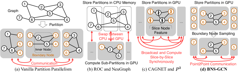
Figure 1: An illustrative comparison between existing distributed GCN training methods and our BNS-GCN.

Sampling-Based GCN Training. Real-world graphs consist of millions of nodes and edges (Hu et al., 2020), far beyond the capability of vanilla GCNs. As such, sampling-based methods were proposed, e.g., neighbor sampling (Hamilton et al., 2017; Chen et al., 2018b), layer sampling (Chen et al., 2018a; Huang et al., 2018; Zou et al., 2019), and subgraph sampling (Chiang et al., 2019; Zeng et al., 2020), which yet suffer from:

• Inaccurate feature estimation: although most sampling methods provide unbiased estimation of node features, the variance of these estimation hurts the model accuracy. As (Cong et al., 2020) shows, a smaller variance is beneficial to improving the accuracy of a sampling-based method;

• Neighbor explosion: Hamilton et al. (2017) first uses node sampling to randomly select several neighbors in the previous layer, but as GCNs get deeper the size of selected nodes exponentially increases. Chen et al. (2018b) further proposes samplers for restricting the size of neighbor expansion, which yet suffers from heavy memory requirements;

• Sampling overhead: All sampling-based methods incur extra time for generating mini-batches, which can occupy 25%+ of the training time (Zeng et al., 2020).

Distributed Training for GCNs. To train GCNs for real-world large graphs, distributed training leveraging multiple GPUs to enable full-graph training has been shown to be promising. Nevertheless, GCNs training is different from the challenge of classical distributed DNN training where (1) data samples are small yet the model is large (model parallelism (Krizhevsky, 2014; Harlap et al., 2018)) and (2) data samples do not have dependency (data parallelism (Li et al., 2020; 2018b; 2018a)), both violating the nature of GCNs. As such, GCN-oriented methods should partition the full graph into small subgraphs such that each could be fitted into a single GPU memory, and train them in parallel, where communication across subgraphs is necessary to exchange boundary node features to perform GCNs’ neighbor aggregation, which is called vanilla partition parallelism as shown in Figure 1(a). Following this paradigm, several works have been proposed. ROC (Jia et al., 2020), NeuGraph (Ma et al., 2019), and AliGraph (Zhu et al., 2019) partition large graphs and store all partitions in CPUs and swaps a fraction of each partition to compute in GPUs (see Figure 1(b)). Their training efficiency are thus compromised due to expensive CPU-GPU swaps. CAGNET (Tripathy et al., 2020) and $P^{3}$ (Gandhi & Iyer, 2021) further split node features and layers to enable intra-layer model parallelism (see Figure 1(c)), which however incurs a heavy communication overhead especially when the feature dimension is large. Dorylus (Thorpe et al., 2021) improves the vanilla partition parallelism by pipelining each fine-grain computation operation in GCN training over numerous CPU threads, which still suffers from the communication bottleneck.

Distributed Graph Systems. Distributed graph systems were proposed to solve general graph problems (Gonzalez et al., 2012; Shun & Blelloch, 2013; Nguyen et al., 2013; Zhu et al., 2016; Chen et al., 2019). (Lerer et al., 2019) also proposes a distributed learning system for graph embedding. However, none of these considers node features and hence cannot be used for GCN training.

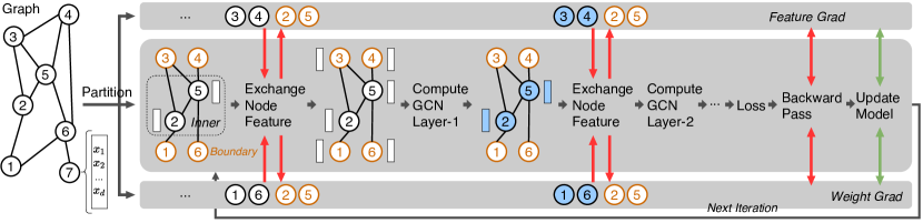
Figure 2: Illustrating vanilla partition parallel training. A large graph is partitioned into smaller subgraphs (see the inner nodes in black) with each being able to fit into one GPU memory. The key challenge is that excessive boundary nodes (in orange) associated with each subgraph (due to GCNs’ neighbor aggregation) can lead to a heavy communication overhead, extra memory cost, and memory imbalance among subgraphs, thus limiting the achievable scalability and efficiency of distributed GCN training.

Table 1: Comparison between the number of boundary nodes and inner nodes in partitioned Reddit graph (Hamilton et al., 2017). The standard METIS (Karypis & Kumar, 1998) is used for graph partition.

Partition Index	1	2	3	4	5	6	7	8	9	10
# Inner Nodes	14k	15k	15k	15k	15k	15k	14k	15k	14k	15k
# Boundary Nodes	39k	15k	86k	78k	86k	62k	6k	46k	71k	23k
Ratio of # Boundary to # Inner	2.64	1.00	5.45	4.95	5.49	4.11	0.42	3.04	4.81	1.52

3 The Proposed BNS-GCN Framework

Overview. To address all aforementioned limitations (see Figure 1(a-c)), we propose partition-parallel training of GCNs with Boundary Node Sampling, dubbed BNS-GCN, as shown in Figure 1(d). BNS-GCN partitions a full-graph with minimized boundary nodes and then further randomly samples the boundary nodes to shrink both communication and memory costs, enabling efficient large-graph training while maintaining the full-graph accuracy. We develop BNS-GCN by first analyzing the three major challenges in partition-parallel training of GCNs and then pinpoint their underlying cause (see Section 3.1). To tackle the cause directly, we design a simple yet effective sampling strategy that can simultaneously alleviate all three challenges (see Section 3), while achieving much reduced variances (i.e., closer to that of the full-graph one) of feature approximation as compared to existing sampling methods (see Section 3.3). We further discuss the difference between BNS-GCN and other sampling-based methods (see Section 3.4) for better understanding our new contribution.

3.1 Challenges in Partition-Parallel Training

To enable full-graph training, the original graph can be partitioned into smaller subgraphs (i.e., partitions) to be trained locally on each accelerator/node while communicating dependent node features across subgraphs, which is termed as partition parallelism. As shown in Figure 2, each subgraph contains a subset of nodes from the original graph, termed as an inner node set (see “Inner”). Additionally, each subgraph holds a boundary node set (see “Boundary”) containing dependent nodes from other subgraphs. Such a boundary node set is dictated by GCNs’ neighbor aggregation from neighbor subgraphs, e.g., node-5 in Figure 2 requires nodes-[3,4,6] residing on other subgraphs to perform Equation 1, creating the boundary nodes associated with the subgraph hosting node-5. To compute each GCN layer, features of boundary nodes are communicated or exchanged across subgraphs (shown in red) before those of inner nodes get updated (e.g., nodes-[2,5] in blue). The updated features are again exchanged across subgraphs to compute the next GCN layer, which is repeated until the final layer. The backward pass follows a similar process but communicates gradients of boundary nodes instead of features. Afterwards, the GCN model gets updated via weight gradient sharing (in green) among partitions using AllReduce.

However, vanilla partition parallelism is neither inefficient nor scalable due to the following three major challenges:

1. Heavy Communication Overhead is resulting from exchanging boundary nodes across partitions, limiting the scalability to larger graphs or using more partitions.

2. Prohibitive Memory Requirement is incurred in each partition to hold both the inner and boundary sets, the latter of which can overflow a GPU’s memory capacity.

3. Imbalanced Memory Requirements exists across all partitions, where the memory straggler (i.e., the partition requiring a significantly larger memory than others) not only determines the memory requirement but also causes under-utilization of other partitions’ GPUs.

We identify that all three challenges above share the same underlying cause – the overhead of extra boundary nodes associated with each partition due to distributed partitions.

Communication Cost Analysis of Vanilla Partition Parallelism. For a partition $\mathcal{G}_{i}$, its communication volume can be defined as $\text{Vol}(\mathcal{G}_{i})=\sum_{v\in\mathcal{G}_{i}}D(v)$ where $D(v)$ is the number of different partitions in which $v$ has at least one neighbor node, excluding $\mathcal{G}_{i}$ (Buluç et al., 2016). This value quantifies the total amount of features $\mathcal{G}_{i}$ needs to send during each propagation (Equation 1). As the total number of received messages equals to the total number of sent messages, the total communication volume equals to the total number of boundary nodes (instead of boundary edges):

$$\text{Vol}_{\text{total}}=\sum_{i}\text{Vol}(\mathcal{G}_{i})=\sum_{i}n_{bd}^{(i)}$$ (3)

where $n_{bd}^{(i)}$ is the number of boundary nodes in partition $\mathcal{G}_{i}$.

Memory Cost Analysis of Vanilla Partition Parallelism. For a $\ell$-th layer, suppose the input feature is of dimension $d^{(\ell)}$, and the numbers of inner nodes and boundary nodes in partition $\mathcal{G}_{i}$ are $n_{in}^{(i)}$ and $n_{bd}^{(i)}$, respectively. Considering a general case where all node features and inner nodes’ aggregated features are saved for the back propagation in both Equation 1 and Equation 2. When using a GraphSAGE layer with a mean aggregator, the memory cost is:

$$\text{Mem}^{(\ell)}(\mathcal{G}_{i})=(3n_{in}^{(i)}+n_{bd}^{(i)})d^{(\ell)}$$ (4)

As a result, the memory requirement increases linearly with the number of boundary nodes (instead of boundary edges).

The challenge is that the number of boundary nodes can be excessive. Table 1 shows a typical example, where the number of boundary nodes in each partition can be as high as $5.5\times$ of that of inner nodes, leading to both prohibitive communication and memory overhead.

Memory Imbalance Analysis in Vanilla Partition Parallelism. The memory cost can be highly imbalanced across partitions due to the irregular amounts of boundary nodes despite the balanced amount of inner nodes (see Table 1). Furthermore, when scaling up to more partitions, the memory imbalance becomes more severe. Figure 3 shows such an example where we split a giant graph (ogbn-papers100M (Hu et al., 2020)) into 192 parts. The memory straggler (the one with boundary-inner ratio of 8) costs significantly more memory than other partitions, which not only raises the memory requirement but also incurs memory under-utilization for all other partitions’ GPUs.

3.2 The Proposed BNS-GCN Technique

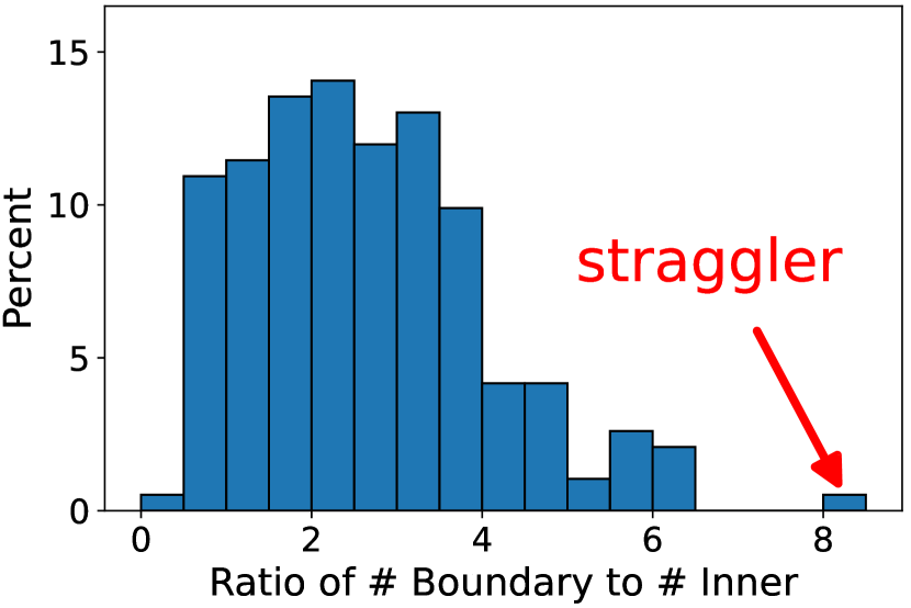
Figure 3: The distributions of the boundary-inner ratios for the ogbn-papers100M dataset under 192 partitions.

Graph Partition. As boundary nodes are the cause for the efficiency bottleneck of partition parallelism, the graph partition has to minimize all boundary node sets to minimize subsequent communication and memory overheads, dubbed Goal-1. Besides, the graph partition must also achieve balanced computation time across all partitions, dubbed Goal-2, since partition parallelism is a synchronous training paradigm that requires frequent synchronization at each layer (again due to GCNs’ neighbor aggregation), under which unbalanced partition results in stragglers that block other partitions to proceed.

Prior works (Tripathy et al., 2020; Zheng et al., 2020) aim at achieving only Goal-2 yet ignore Goal-1, while this work achieves both. For Goal-2, we approximate the computational complexity of each node, aiming to balance computations across all partitions (e.g., when GraphSAGE computation is dominated by Equation 2, the complexity is proportional to the number of nodes, so we set partitions with an equal size in this case). Then we optimize the graph partition algorithm for Goal-1. In this work, the popular METIS (Karypis & Kumar, 1998) is adopted as the default graph partition algorithm and its objective is set to minimize the communication volume, i.e., minimize the number of boundary nodes (Equation 3). Besides METIS, other partitioning algorithms are also compatible with BNS-GCN (see Tables 7-8). Note that the time complexity of METIS is $\mathcal{O}(|\mathcal{E}|)$ where $\mathcal{E}$ is the set of edges, and only needs to be performed once during the preprocessing stage, the cost of which can thus be amortized over numerous training iterations and leads to a negligible overhead. In addition, METIS is widely adopted in scalable GCN training (Zhu et al., 2019; Zheng et al., 2020; Fey et al., 2021; Wan et al., 2022) where the objective function is mostly set as the minimum cut (i.e., minimize the number of edges).

Input: partition number $m$, partition id $i$, graph partition $\mathcal{G}_{i}$, boundary node set $\mathcal{B}_{i}$, node feature $X_{i}$, label $Y_{i}$, sampling rate $p$, initial model $w[0]$, learning rate $\eta$

Output: trained model $w[T]$ after $T$ iterations

$\mathcal{V}_{i}\leftarrow\{\text{node }v\in\mathcal{G}_{i}:v\notin\mathcal{B}_{i}\}$;

  $\triangleright$ create inner node set

$H^{(0)}\leftarrow X_{i}$;

  $\triangleright$ initialize input features

1 for $t\leftarrow 1:T$ do

2       $\mathcal{U}_{i}\leftarrow$ randomly pick elements in $\mathcal{B}_{i}$ with probability $p$;

3      

4      $\mathcal{H}_{i}\leftarrow$ node induced subgraph of $\mathcal{G}_{i}$ from $\mathcal{V}_{i}\cup\mathcal{U}_{i}$;

5      

6      Broadcast $\mathcal{U}_{i}$ and Receive $[\mathcal{U}_{1},\cdots,\mathcal{U}_{m}]$;

7      

8      $[\mathcal{S}_{i,1},\cdots,\mathcal{S}_{i,m}]\leftarrow[\mathcal{U}_{1}\cap\mathcal{V}_{i},\cdots,\mathcal{U}_{m}\cap\mathcal{V}_{i}$];

9      

10      for $\ell\leftarrow 1:L$ do

11             Send $[H_{\mathcal{S}_{i,1}}^{(\ell-1)},\cdots,H_{\mathcal{S}_{i,m}}^{(\ell-1)}]$ to partition $[1,\cdots,m]$ and Receive $H_{\mathcal{U}_{i}}^{(\ell-1)}$;

12            

13            $H^{(\ell)}\leftarrow GCN^{(\ell)}\left(\mathcal{H}_{i},\left[\begin{array}[]{c}H^{(\ell-1)}\\ H_{\mathcal{U}_{i}}^{(\ell-1)}\end{array}\right],w[t-1]\right)$;

14            

15       end for

      $f_{i}\leftarrow\sum_{v\in\mathcal{V}_{i}}loss(h_{v}^{(L)},y_{v})$;

        $\triangleright$ calculate loss

       $g_{i}[t]\leftarrow\frac{\partial f_{i}}{\partial w[t-1]}$;

        $\triangleright$ backward pass

       $g[t]\leftarrow AllReduce(g_{i}[t])$;

        $\triangleright$ share gradients

       $w[t]\leftarrow w[t-1]-\eta\cdot g[t]$;

        $\triangleright$ update model

16      

17 end for

return $w[T]$

Algorithm 1 Boundary node sampling for partition-parallel training (per-partition view)

Boundary Node Sampling (BNS). Even with an optimal graph partition, the boundary node issue still remains (see Table 1), calling for innovative methods to reduce the boundary node volume. An ideal method should achieve three goals: (1) substantially shrinking the size of boundary node sets, (2) incurring a minimal overhead, and (3) maintaining the full-graph accuracy. As such, we adopt a random sampling method called boundary node sampling. The key idea is to independently select a subset of boundary nodes from each partition, then to store and communicate merely those selected ones instead of the full boundary sets, with a random selection varying from one epoch to another.

Table 2: Comparing feature approximation variance between SOTA sampling methods and BNS-GCN, where we fix the target node set $\mathcal{V}_{i}$ across all methods. Here $\gamma$ denotes the upper bound of the $L_{2}$-norm of intermediate features, and $\Delta\gamma$ is the upper bound of the difference between the embedding feature and its history. We report the variance by ignoring the same factors. Note that $\left|\mathcal{B}_{i}\right|\ll\left|\mathcal{N}_{i}\right|\ll\left|\mathcal{V}\right|$.

Method	Variance	Notation
GraphSAGE	$\mathcal{O}(D\gamma^{2}/s_{n})$	$s_{n}$: sampled neighbor size $D$: average degree
VR-GCN	$\mathcal{O}(D\Delta\gamma^{2}/s_{n})$
FastGCN	$\mathcal{O}(|\mathcal{V}|\gamma^{2}/s_{\ell})$	$s_{\ell}$: sampled node set size $\mathcal{V},\mathcal{N}_{i},\mathcal{B}_{i}$: global node set, neighbor set, boundary set
LADIES	$\mathcal{O}(|\mathcal{N}_{i}|\gamma^{2}/s_{\ell})$
BNS-GCN	$\mathcal{O}(|\mathcal{B}_{i}|\gamma^{2}/s_{\ell})$

Algorithm 1 outlines our proposed BNS-GCN. In the $i$-th partition, we randomly keep the boundary node set $\mathcal{U}_{i}$ with a probability $p$ and drop the rest at the beginning of each epoch (Lines 1-1). These selected nodes’ indices are then broadcasted among partitions such that each partition “knows” others’ selections (Line 1) and can also record its local node $\mathcal{S}_{i,j}$ that is selected by the other $j$-th partition (Line 1). During the forward pass of the $\ell$-th layer, each partition sends those features $H^{(\ell-1)}_{\mathcal{S}_{i,j}}$ of the previously recorded nodes to the corresponding $j$-th partition and meanwhile receives features $H^{(\ell-1)}_{\mathcal{U}_{i}}$ of its own selected boundary nodes to perform GCN operations (Lines 1-1). For a mean aggregator, we replace the sent/received feature matrix $H$ with $H/p$ towards an unbiased feature estimation. During the backward pass of every layer, each partition sends and receives feature gradients of the selected boundary nodes while generating GCNs’ weight gradients (Line 1). Lastly, weight gradients are shared across partitions via AllReduce (Thakur et al., 2005) to perform weight updates (Lines 1-1).

The proposed BNS-GCN reduces the number of boundary nodes by a factor of $\frac{1}{p}$, achieving a proportional reduction in both memory and communication costs (Equation 3-4). Meanwhile, BNS-GCN pays negligible overhead due to its simplicity, which costs 0%$\sim$7% of the training time in practice. Note that our BNS-GCN can not only boost the efficiency and scalability of vanilla partition parallelism, but also be easily plugged into any partition-parallel training methods (e.g., ROC and CAGNET) for further improving their training efficiency.

3.3 Variance Analysis

Theoretically, we study the effect of BNS-GCN on GCNs’ performance by analyzing its feature approximation variance and comparing it with the SOTA methods. As the feature approximation variance controls the upper bound of gradient noise (Cong et al., 2020), a sampling method with a lower approximation variance usually enjoys a better convergence speed (Gower et al., 2019) and higher accuracy. Table 3.2 summarizes our results, where $\mathcal{V}$, $\mathcal{N}_{i}$, and $\mathcal{B}_{i}$ denote the global node set, neighbor set, and boundary neighbor set, respectively. The detailed variance analysis of BNS-GCN can be found in Appendix A and variances for the other methods are based on (Zou et al., 2019). We find that BNS-GCN enjoys the smallest variance compared with FastGCN and LADIES, when fixing the number of sampled nodes, as we strictly have $\mathcal{B}_{i}\subseteq\mathcal{N}_{i}\subseteq\mathcal{V}$. To be able to compare with GraphSAGE, we fix the sampling size ($s_{\ell}$ = $s_{n}$), then BNS-GCN is strictly better than GraphSAGE, as BNS-GCN neither samples neighbors within the inner node sets nor samples the same nodes for multiple times, leading to $|\mathcal{B}_{i}|\leq D|\mathcal{V}_{i}|$. For VR-GCN, it is not comparable with BNS-GCN because the variance of VR-GCN is based on the difference between embedding feature and its history.

3.4 BNS-GCN vs. Existing Sampling Methods

We further discuss the difference between BNS-GCN and existing sampling methods:

• Node Sampling: GraphSAGE (Hamilton et al., 2017) and VR-GCN (Chen et al., 2018b) adopt node sampling which is likely to sample the same nodes multiple times from the previous layers, limiting GCNs’ depth and training efficiency. Additionally, BNS-GCN does not sample neighbors within each subgragh, reducing both the estimation variance and sampling overhead.

• Layer Sampling: BNS-GCN is similar to layer sampling in that nodes within the same partition share the same sampled boundary nodes in the previous layer. Unlike FastGCN (Chen et al., 2018a), AS-GCN (Huang et al., 2018) or LADIES (Zou et al., 2019), BNS-GCN has much denser sampled layers, potentially leading to a higher accuracy.

• Subgraph Sampling: BNS-GCN could be viewed as one kind of subgraph sampling that drops boundary nodes from other partitions. ClusterGCN (Chiang et al., 2019) and GraphSAINT (Zeng et al., 2020) propose subgraph sampling, yet their number of selected nodes are small, i.e., only 1.3% and 5.3% of the total nodes, respectively, causing a higher variance of gradient estimation.

• Edge Sampling: Applying edge sampling (e.g., DropEdge (Rong et al., 2019)) to distributed GCN training is not efficient, as it does not directly reduce the number of boundary nodes (see Section 4.3).

Table 3: Details of the graph datasets.

Dataset	# Nodes	# Edges	# Feat.	# Classes	Type	Train / Val / Test
Reddit (Hamilton et al., 2017)	233K	114M	602	41	inductive	0.66 / 0.10 / 0.24
ogbn-products (Hu et al., 2020)	2.4M	62M	100	47	transductive	0.08 / 0.02 / 0.90
Yelp (Zeng et al., 2020)	716K	7.0M	300	100	inductive	0.75 / 0.10 / 0.15
ogbn-papers100M (Hu et al., 2020)	111M	1.6B	128	172	transductive	0.78 / 0.08 / 0.14

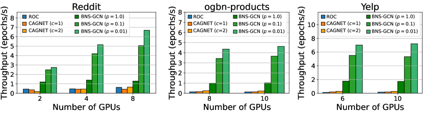
Figure 4: Throughput comparison on Reddit, ogbn-products, and Yelp. Each partition uses one GPU (except CAGNET ($c=2$) uses two). The boundary node sampling rate is denoted by $p$.

4 Experiments

In this section, we first introduce our experiment setups, then compare with the SOTA baselines, and further provide ablation studies for a thorough evaluation on BNS-GCN.

Datasets. We evaluate BNS-GCN on four large-scale datasets: 1) Reddit (Hamilton et al., 2017) for community prediction based on the posts’ contents and users’ comments, 2) ogbn-products (Hu et al., 2020) for classifing Amazon products based on customers’ review, 3) Yelp (Zeng et al., 2020) for predicting the types of business based on reviews and users’ relationship, and 4) ogbn-papers100M (Hu et al., 2020) for predicting the category of an arXiv publication based on its title and abstract. Details of these four datasets are provided in Table 3.

Models. We adopt a GraphSAGE model with an Adam optimizer for all datasets. The details are listed below:

• Reddit: We use a 4-layer model with 256 hidden units and set the learning rate as 0.01 with 3000 epochs and 0.5 dropout rate.

• ogbn-products: We use a 3-layer model with 128 hidden units and set the learning rate as 0.003 with 500 epochs and 0.3 dropout rate.

• Yelp: We use a 4-layer model with 512 hidden units and set the learning rate as 0.001 with 3000 epochs and 0.1 dropout rate.

• ogbn-papers100M: We use a 3-layer model with 128 hidden units and set the learning rate as 0.01 with 100 epochs and 0.5 dropout rate.

Setups. We implement BNS-GCN in DGL (Wang et al., 2019) and PyTorch (Paszke et al., 2019) with the default backend of Gloo. We conduct the experiments of Reddit, ogbn-products and Yelp on a machine with 10 RTX-2080Ti (11GB), Xeon 6230R@2.10GHz (187GB), and PCIe3x16 connecting CPU-GPU and GPU-GPU. The minimal number of partitions for full-graph training are 2, 5, 3 for Reddit, ogbn-products, and Yelp, respectively. For ogbn-papers100M, the experiment is conducted on 32 machines, each of which has 6 Tesla V100 (16GB) with IBM Power9 (605GB). To ensure the reproducibility and robustness of BNS-GCN, we do not tune but fix the hyper-parameters for BNS-GCN throughout all experiments, and we show evaluation results based on average of 10 runs.

Table 4: Comparison of test accuracy (%) on Reddit and ogbn-products and of test F1-micro score (%) on Yelp.

Method	Reddit			ogbn-products			Yelp
Sampling-based methods
FastGCN (Chen et al., 2018a)	93.7			60.42			26.5
GraphSAGE (Hamilton et al., 2017)	95.4			78.70			63.4
AS-GCN (Huang et al., 2018)	96.3			OOM∗			OOM∗
LADIES (Zou et al., 2019)	94.3			77.46			60.2
VR-GCN (Chen et al., 2018b)	96.3			OOM∗			64.0
ClusterGCN (Chiang et al., 2019)	96.6			78.97			60.9
GraphSAINT (Zeng et al., 2020)	96.6			79.08			65.3
BNS-GCN
# Partitions	2	4	8	5	8	10	3	6	10
BNS-GCN ($p=1.0$)	97.11	97.11	97.11	79.14	79.14	79.14	65.26	65.26	65.26
BNS-GCN ($p=0.1$)	97.17	97.16	97.15	79.36	79.48	79.30	65.32	65.26	65.34
BNS-GCN ($p=0.01$)	97.09	96.99	96.94	79.43	79.28	79.21	65.27	65.31	65.29
BNS-GCN ($p=0.0$)	97.03	96.88	96.84	78.65	78.83	78.79	65.28	65.27	65.23

4.1 Comparison with the SOTA Baselines

Full-Graph Training Speedup. Figure 4 compares the training throughput of BNS-GCN against the SOTA full-graph training methods, ROC (Jia et al., 2020) and CAGNET (Tripathy et al., 2020). We observe that BNS-GCN consistently outperforms both baselines across different number of GPUs and boundary node sampling rates $p$. For the instance of training GCN on Reddit, BNS-GCN with $p=0.01$ offers a promising throughput improvement of 8.9$\times$$\sim$16.2$\mathbf{\times}$ over ROC and 9.2$\times$$\sim$13.8$\times$ over CAGNET ($c=2$) across different number of GPUs. Even when $p=1$, BNS-GCN still improves the throughput by 1.8$\times$$\sim$3.7$\times$ over ROC and 1.0$\times$$\sim$5.5$\times$ over CAGNET ($c=2$). The advantage of BNS-GCN is attributed to not only the reduced communication overhead with boundary node sampling, but also no swap between CPU and GPU as ROC nor redundant broadcast and synchronization overhead as CAGNET. Furthermore, increasing the number of partitions boosts the performance of BNS-GCN ($p<1$) substantially, but not for other methods, validating BNS-GCN’s advantageous scalability thanks to its effectiveness in reducing communication overhead by dropping boundary nodes. The advantage of BNS-GCN is similar for the other two datasets.

Full-Graph Accuracy. Now we show that BNS-GCN maintains or even improves the accuracy of full-graph training, while boosting the training efficiency. Table 4 summarizes our extensive evaluations of test scores when BNS-GCN adopts various sampling rates and different numbers of partitions, and compare with seven SOTA sampling-based methods (Hu et al., 2020; with Code, 2020; Chiang et al., 2019; Chen et al., 2018b; Zeng et al., 2020; Hamilton et al., 2017; Cong et al., 2020; Liu et al., 2022; Zou et al., 2019; Chen et al., 2020). We observe that full-graph training (BNS-GCN with $p=1$) always achieves a higher or comparable accuracy than existing sampling-based methods, regardless of datasets or number of partitions, which is consistent with the results of ROC (Jia et al., 2020). More importantly, BNS-GCN always maintains or even increases the full-graph accuracy, regardless of the sampling rates (e.g., $p=0.1/0.01$), the number of partitions, or different datasets. For instance, on Reddit, $p=0.1$ achieves a test accuracy of 97.15%$\sim$97.17% under 2$\sim$8 partitions, which are consistently better than the 97.11% accuracy of full-graph unsampled training, validating the effectiveness and robustness of BNS-GCN. Meanwhile, we also observe that the special case of BNS-GCN, $p=0$, always suffers from the worst test score on the three datasets, compared with other cases ($p>0$). We understand that this accuracy/score drop is due to the full isolation of each partition after completely removing all boundary nodes, leading to no boundary node features during neighbor aggregation throughout the end-to-end training. To the best of our knowledge, BNS-GCN achieves the best accuracy of training GraphSAGE-layer based GCNs on all three datasets compared with all existing works.

Table 5: Comparison between BNS-GCN (10 partitions) and sampling-based methods on ogbn-products.

Method	Total Train Time	Test Acc (%)
ClusterGCN	294.2s	78.97±0.33
NeighborSampling	281.8s	78.70±0.36
GraphSAINT	157.4s	79.08±0.24
BNS-GCN ($p=1.0$)	269.1s	79.14±0.35
BNS-GCN ($p=0.1$)	155.3s	79.30±0.36
BNS-GCN ($p=0.01$)	142.9s	79.21±0.26

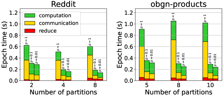
Figure 5: Training time breakdown of BNS-GCN with different boundary node sampling rates $p$.

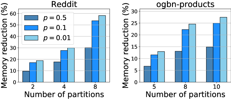
Figure 6: Memory usage reduction achieved by BNS-GCN, where the reduction is against $p=1.0$.

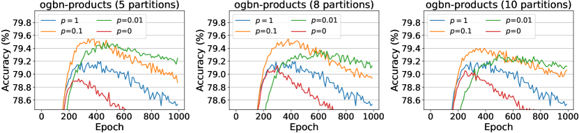
Figure 7: Test-accuracy convergence comparison among unsampled full-graph training (BNS-GCN with $p=1$), boundary-node sampled training ($p=0.1/0.01$), and isolated training ($p=0$) on ogbn-products.

Improvement over Sampling-based Methods. Besides the full-graph training comparison, we also validate BNS-GCN’s advantage over the SOTA sampling-based methods (implemented by the OGB team (Hu et al., 2020)) on ogbn-products as shown in Table 5. We observe that BNS-GCNs with $p=0.1$ and $p=0.01$ outperform all the sampling-based methods in terms of both efficiency and accuracy thanks to its lower approximation variance and substantially higher achieved throughput. More comparisons between BNS-GCN and sampling-based methods can be found in Appendix C.

4.2 Performance Analysis

Training Time Improvement Breakdown. To further understand the improvement of BNS-GCN, we breakdown the training time into three major components (local computation, communication for boundary nodes, and allreduce on model gradient) as shown in Figure 6. We observe that communication dominates the training time (up to 67% and 64% in baselines ($p=1$) on Reddit and obgn-products, respectively). As expected, with boundary node sampling ($p<1$), the communication overhead is substantially reduced, thus the total training time is improved. Specifically, $p=0.01$ sharply cuts 74%$\sim$93% and 83%$\sim$91% of the communication time from that of the baselines on Reddit and obgn-product, respectively, where this benefit consistently holds as the number of partitions scales. Furthermore, in addition to single machine training, we also study BNS-GCN’s benefits for multi-machine training and evaluate the performance on ogbn-papers100M. Specifically, we separate ogbn-papers100M into 192 parts and deploy the training on 32 machines (6 GPUs per machine), and provide results in Table 6. We can see that BNS-GCN with $p=0.01$ considerably reduce the total training time by 99%, showing that distributed GCN training with multiple machines suffers from a more severe communication bottleneck and thus making BNS-GCN more desirable.

Table 6: Epoch time breakdown of ogbn-papers100M.

Method	Total	Comp.	Comm.	Reduce
BNS-GCN ($p=1.0$)	554.1s	5.3s	550.3s	0.8s
BNS-GCN ($p=0.1$)	58.7s	1.0s	56.9s	0.8s
BNS-GCN ($p=0.01$)	6.0s	0.6s	4.8s	0.6s

Memory Saving. BNS-GCN’s advantage in terms of memory usage reduction is shown in Figure 6. We observe that BNS-GCN consistently reduces the memory usage across different number of partitions on both graphs. Specifically, for the denser Reddit graph (with an average node degree of 984.0), $p=0.01$ saves 58% memory usage for 8 GPUs. Even for the sparser obgn-products graph (with an average node degree of 50.5), $p=0.01$ still saves 27% memory usage for 10 GPUs. Note that the memory saving of BNS-GCN scales with the numbers of partition, because the number of boundary nodes increases with more partitions, indicating BNS-GCN’s scalability to training larger graphs. Also, we find that BNS-GCN’s memory reduction is not linear with reduced $p$, as besides the tensors analyzed in Equation 4 there are other objects (e.g., caches for non-linear activations and dropout) occupying the memory during training.

Table 7: Test score (%) of BNS-GCN on top of random partition, where +/- shows the accuracy difference from BNS-GCN on top of METIS in Table 4.

Method	Reddit (8 partitions)		ogbn-products (10 partitions)		Yelp (10 partitions)
Random+BNS ($p=1.0$)	97.11	+0.00	79.14	+0.00	65.26	+0.00
Random+BNS ($p=0.1$)	96.95	-0.20	79.57	+0.27	65.18	-0.16
Random+BNS ($p=0.0$)	93.37	-3.47	75.39	-3.40	64.92	-0.31

Table 8: Training efficiency improvement of BNS-GCN ($p=0.1$) on top of different partition methods.

Dataset	Throughput		Memory		# Boundary Nodes
	METIS	Random	METIS	Random	METIS	Random
Reddit (8 partitions)	3.1$\times$	5.0$\times$	0.47$\times$	0.36$\times$	460k	1,016k
ogbn-products (10 partitions)	3.4$\times$	7.3$\times$	0.75$\times$	0.31$\times$	1,848k	16,797k
Yelp (10 partitions)	3.1$\times$	5.1$\times$	0.83$\times$	0.49$\times$	649k	2,026k

Generalization Improvement. To understand the effect of BNS-GCN’s generalization capability, we also evaluate the test-accuracy convergence in Figure 7. Here ogbn-products is adopted as the study case because the distribution of its test set largely differs from that of its training set (Hu et al., 2020). From Figure 7, we observe that full-graph training without boundary node sampling ($p=1$) or completely isolated training ($p=0$) can overfit rapidly, regardless of different number of partitions. With boundary node sampling ($p=0.1/0.01$), this overfitting issue is mitigated, i.e., both the convergence and the optimality are improved substantially and consistently across different number of partitions. This is because BNS-GCN randomly modifies the graph throughout end-to-end training. More convergence curves on other datasets can be found in Appendix B.

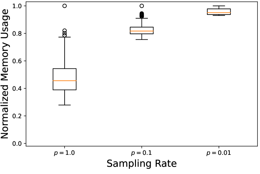
Figure 8: Normalized per-partition memory usage on ogbn-papers100M (192 partitions). The normalization is against the highest memory partition and is separated for different sampling rates $p$ of BNS-GCN.

Balanced Memory Usage. To validate the benefit of BNS-GCN in balancing memory usage across partitions, we measure per-partition memory usage of ogbn-papers100M with 192 partitions and show their box plots in Figure 8. We observe that the unsampled case ($p=1.0$) suffers from a severe memory imbalance, where one straggler increases the memory requirement by around 20% and more than three-fourths partitions occupy less than 60% memory. By contrast, with boundary node sampling, $p=0.1/0.01$ balances the memory usage and thus better utilizes memory resource, i.e., all partitions leverage more than 70% memory.

Table 9: Comparison between BNS-GCN and edge sampling methods, DropEdge and Boundary Edge Sampling (BES).

Dataset	Method	Epoch Comm (MB)	Epoch Time (sec)	Test Score (%)
Reddit (2 partitions)	DropEdge	301.3	0.613	97.12
	BES	207.9	0.484	97.16
	BNS-GCN	30.4	0.319	97.17
ogbn-products (5 partitions)	DropEdge	1364.0	0.938	79.38
	BES	521.1	0.551	79.31
	BNS-GCN	138.7	0.388	79.36
Yelp (3 partitions)	DropEdge	718.7	0.606	65.30
	BES	195.3	0.328	65.30
	BNS-GCN	75.7	0.270	65.32

4.3 Ablation Studies

BNS-GCN with Random Partition. To further understand the effectiveness of BNS-GCN and whether it relies on the adopted METIS partitioner, we conduct an ablation study by replacing METIS with random partition (i.e., randomly assign nodes to each partition without optimization) and provide the resulting accuracy in Table 7. We observe that when $p=0.1$, i.e., sampling normally, random partition plus BNS-GCN still offers a comparable performance (-0.20$\sim$+0.27) as the original METIS plus BNS-GCN, thus showing that the proposed BNS-GCN is orthogonal to the adopted graph partitioning technique and is not necessarily limited to METIS. We further study whether BNS-GCN consistently improves training efficiency on top of different partition algorithms, and demonstrate the result in Table 8. We observe that random partition gains more benefits in throughput improvement and memory saving from BNS-GCN ($p=0.1$) than the METIS, because the former partitioner creates more boundary nodes.

The Special Case $p=0$. The special case of the proposed boundary node sampling, $p=0$, is not recommended to use in practice. First, $p=0$ always suffers from the worst test accuracy/score (compared with other cases ($p>0$)) on all datasets and with different partition methods (see Table 4 and Table 7). Specifically, with random partition, $p=0$ drops the test accuracy on Reddit from 97.11% ($p=1$) to 93.37% (lower than FastGCN (Chen et al., 2018a)). This drop is due to the absolute isolation of each partition after completely removing all boundary nodes, leading to no boundary node features during neighbor aggregation (Equation 1) throughout the end-to-end training. Second, $p=0$ also suffers from the slowest convergence regardless of different numbers of partitions or different datasets. Third, $p=0$ overfits severely (see Figure 7). Therefore, we suggest a small but non-zero sampling rate ($p=0.1/0.01$). More discussion regarding the choice of sampling rate can be found in Appendix E.

BNS-GCN vs. Boundary Edge Sampling. As many works (Zhu et al., 2019; Zheng et al., 2020; Fey et al., 2021) assume that communication overhead of distributed GCN training is caused by the inter-partition edges (rather than boundary nodes) and thus pursuing a minimal edge cut, one could reduce communication overhead by cutting edges using sampling techniques like DropEdge (Rong et al., 2019) or even an enhanced version that samples only the boundary edges (rather than at a global scale). To understand this, we implemented the enhanced version, dubbed Boundary Edge Sampling (BES), and apply both BES and DropEdge to the partition-parallel training. Table 9 compares their performance with BNS-GCN. For a fair comparison, all methods drop the same number of edges with BNS-GCN ($p=0.1$) over the full graph. We observe that edge-based sampling methods are ineffective. For Reddit, DropEdge and BES cause 10$\times$ and 7$\times$ communication overhead of BNS-GCN, and thus 2.0$\times$ and 1.4$\times$ the overall training time. This is because, in real-world graphs, multiple boundary edges can connect to the same boundary nodes. Even if we drop some of those edges, the remaining undropped edges still demand communicating the connected boundary nodes to satisfy neighbor aggregation of GCNs. Obviously, to eradicate such communication costs, boundary nodes should be directly targeted and dropped, instead of using boundary edges. For ogbn-products and Yelp, the advantage of BNS-GCN still holds, where BNS-GCN reduces up to 90% communication volume and speeds up training time by up to 2.4$\times$. Analytically, we’ve shown that the communication cost of distributed GCN training is only proportional to the number of boundary nodes (see Equation 3).

Table 10: Epoch training time speedup on GAT.

BNS-GCN	Reddit	ogbn-products	Yelp
$p=1$	1.00$\times$ (0.84s)	1.00$\times$ (0.71s)	1.00$\times$ (0.33s)
$p=0.1$	1.53$\times$	1.78$\times$	1.83$\times$
$p=0.01$	1.58$\times$	1.91$\times$	2.06$\times$
$p=0$	1.68$\times$	2.03$\times$	2.20$\times$

BNS-GCN Benefit on GAT. To validate the general applicability of BNS-GCN across different types of GCN models (i.e., not just GraphSAGE), we train GAT (Veličković et al., 2017) with BNS-GCN and provide the improvement for a 2-layer GAT with 10 partitions in Table 10. We observe that BNS-GCN is consistently effective and speedups the training by 58%$\sim$106%, despite GAT being more computationally intensive than GraphSAGE.

5 Conclusion

While training GCNs at scale is challenging and increasingly important, existing methods for distributed GCN training are still limited in their achievable performance and scalability. This work takes the initial effort to analyze the three major challenges in distributed GCN training and then identify their underlying cause. On top of that, we propose an efficient and scalable method for full-graph GCN training, BNS-GCN, and then validate its effectiveness through both theoretical analysis and extensive empirical evaluations. We believe that these findings and the proposed method have provided a better understanding of distributed GCN training and will inspire further innovations in this direction.

ACKNOWLEDGEMENT

The work is supported by the National Science Foundation (NSF) through the MLWiNS program (Award number: 2003137), the CC^∗ Compute program (Award number: 2019007) and the NeTS program (Award number: 1801865).

Appendix A The Variance Analysis

In this section, we derive the variance of embedding approximation when using our proposed BNS-GCN method, of which the result is listed in Table 3.2 of the main content.

For a given graph $\mathcal{G}=(\mathcal{V},\mathcal{E})$ with an adjacency matrix $A$, we define the propagation matrix $P$ as $P=\tilde{D}^{-1/2}\tilde{A}\tilde{D}^{-1/2}$, where $\tilde{A}=A+I,\tilde{D}_{u,u}=\sum_{v}\tilde{A}_{u,v}$. One GCN layer performs one step of feature propagation (Kipf & Welling, 2016) as formulated below:

$$Z^{(\ell)} =PH^{(\ell-1)}W^{(\ell-1)}$$ (5)

$$H^{(\ell)} =\sigma\left(Z^{(\ell)}\right)$$

where $H^{(\ell)}$, $W^{(\ell)}$, and $Z^{(\ell)}$ denote the embedding matrix, the trainable weight matrix, and the intermediate embedding matrix in the $\ell$-th layer, respectively, and $\sigma$ denotes the non-linear function. Without loss of generality, we provide our analysis for one layer of GCNs and drop the superscripts of $(\ell)$ and $(\ell-1)$ in the reminder of the discussion for simplicity.

For distributed GCN training using partition-parallelism, if denoting the inner node set and the boundary node set of the $i$-th partition as $\mathcal{V}_{i}$ and $\mathcal{B}_{i}$, respectively, the operations of the $i$-th partition for calculating Equation 5 are as follows: Z_V_i,*= [PVi,ViPVi,Bi] [HVi,*HBi,*]W

In BNS-GCN, $Z_{\mathcal{V}_{i},*}$ is approximated as $\tilde{Z}_{\mathcal{V}_{i},*}$ due to its boundary node sampling, i.e.,

~Z_V_i,*= [PVi,ViPVi,Ui] S [HVi,*HUi,*]W where $\mathcal{U}_{i}$ denotes the sampled boundary node set, $p$ denotes the sampling rate, and $S$ is a diagnal matrix with its elements being defined as:

$$S_{u,u}=\begin{cases}1,&u\leq|\mathcal{V}_{i}|\\ 1/p,&u>|\mathcal{V}_{i}|\end{cases}$$

Similar to the variance analysis in (Chen et al., 2018b) and (Zou et al., 2019), our goal is to compute the average variance of the approximated embedding for one GCN layer, which can be defined as $\mathbb{E}_{\mathcal{U}}[\|\tilde{Z}-Z\|_{F}^{2}]/|\mathcal{V}|$. In our analysis, we adopt the same assumption as that in (Zou et al., 2019), which bounds the matrix product $HW$ as follows:

Assumption A.1.

We assume that the $L_{2}$-norm of each row in HW is upper bounded by a constant, i.e., there exists a constant $\gamma$ such that $\|H_{u,*}W\|_{2}\leq\gamma$ for all $u\in\left|\mathcal{V}\right|$.

Next, we calculate the total variance of the embedding approximation for the $i$-th partition:

$$\mathbb{E}_{\mathcal{U}_{i}}[\|\tilde{Z}_{\mathcal{V}_{i},*}-Z_{\mathcal{V}_{i},*}\|_{F}^{2}] =\mathbb{E}_{\mathcal{U}_{i}}\left[\left\|\begin{bmatrix}P_{\mathcal{V}_{i},\mathcal{V}_{i}}&P_{\mathcal{V}_{i},\mathcal{U}_{i}}\end{bmatrix}S\begin{bmatrix}H_{\mathcal{V}_{i},*}\\ H_{\mathcal{U}_{i},*}\end{bmatrix}W-\begin{bmatrix}P_{\mathcal{V}_{i},\mathcal{V}_{i}}&P_{\mathcal{V}_{i},\mathcal{B}_{i}}\end{bmatrix}\begin{bmatrix}H_{\mathcal{V}_{i},*}\\ H_{\mathcal{B}_{i},*}\end{bmatrix}W\right\|_{F}^{2}\right]$$

$$=\mathbb{E}_{\mathcal{U}_{i}}\left[\left\|\frac{1}{p}P_{\mathcal{V}_{i},\mathcal{U}_{i}}H_{\mathcal{U}_{i},*}W-P_{\mathcal{V}_{i},\mathcal{B}_{i}}H_{\mathcal{B}_{i},*}W\right\|_{F}^{2}\right]$$ (6)

$$=\sum_{v\in\mathcal{V}_{i}}\mathbb{E}_{\mathcal{U}_{i}}\left[\left\|\sum_{u\in\mathcal{U}_{i}}\frac{1}{p}P_{v,u}H_{u,*}W-P_{v,\mathcal{B}_{i}}H_{\mathcal{B}_{i},*}W\right\|_{2}^{2}\right]$$

$$=\sum_{v\in\mathcal{V}_{i}}\frac{1}{p}\sum_{u\in\mathcal{B}_{i}}\left\|P_{v,u}H_{u,*}W-\frac{1}{|\mathcal{B}_{i}|}P_{v,\mathcal{B}_{i}}H_{\mathcal{B}_{i},*}W\right\|_{2}^{2}$$ (7)

$$=\sum_{v\in\mathcal{V}_{i}}\frac{1}{p}\left(\sum_{u\in\mathcal{B}_{i}}\left\|P_{v,u}H_{u,*}W\right\|_{2}^{2}-\left\|P_{v,\mathcal{B}_{i}}H_{\mathcal{B}_{i},*}W\right\|_{2}^{2}\right)$$

$$\leq\frac{1}{p}\sum_{v\in\mathcal{V}_{i}}\sum_{u\in\mathcal{B}_{i}}\left\|P_{v,u}H_{u,*}W\right\|_{2}^{2}$$

where the step of Equation 6 removes the common factor $P_{\mathcal{V}_{i},\mathcal{V}_{i}}H_{\mathcal{V}_{i},*}W$ and the step of Equation 7 uses the fact that the selection of nodes in $\mathcal{B}_{i}$ are independent.

Based on Assumption A.1, we have $\left\|H_{u,*}W\right\|_{2}\leq\gamma$. As a result, the above upper bound can be further written as:

$$\mathbb{E}_{\mathcal{U}_{i}}[\|\tilde{Z}_{\mathcal{V}_{i},*}-Z_{\mathcal{V}_{i},*}\|_{F}^{2}] \leq\frac{1}{p}\sum_{v\in\mathcal{V}_{i}}\sum_{u\in\mathcal{B}_{i}}P_{v,u}^{2}\gamma^{2}$$

$$=\frac{1}{p}\gamma^{2}\left\|P_{\mathcal{V}_{i},\mathcal{B}_{i}}\right\|_{F}^{2}$$

Thus, the total variance of the embedding approximation for the $i$-th partition is $\mathcal{O}(|\mathcal{B}_{i}|\gamma^{2}/s_{\ell})$ as shown in Table 3.2 of the main content, where $s_{\ell}$ denote the size of the sampled node set.

Finally, the global average variance can be calulated as:

$$\frac{\mathbb{E}_{\mathcal{U}}[\|\tilde{Z}-Z\|_{F}^{2}]}{|\mathcal{V}|} =\frac{\sum_{i}\mathbb{E}_{\mathcal{U}_{i}}[\|\tilde{Z}_{\mathcal{V}_{i},*}-Z_{\mathcal{V}_{i},*}\|_{F}^{2}]}{|\mathcal{V}|}$$

$$\leq\frac{\gamma^{2}\sum_{i}\left\|P_{\mathcal{V}_{i},\mathcal{B}_{i}}\right\|_{F}^{2}}{p|\mathcal{V}|}$$

$$\leq\frac{\gamma^{2}\|P\|_{F}^{2}}{p|\mathcal{V}|}$$

Appendix B Convergence Speedup (Additional Experiments)

Figure 9 shows convergence speedups of BNS-GCN on more datasets under the same setting of Figure 7 of the main content. The observations from the main content still hold. Especially, boundary node sampling at a high rate ($p=0.1$) achieves the best convergence regardless of different numbers of partitions or different datasets. A lower rate ($p=0.01$) still remains a close convergence as $p=0.1$. The special case $p=0$ suffers from not only the worst convergence but also increased convergence gap between $p=0$ and $p=0.1$ as more partitions are involved, because of complete removal of boundary node information. Lastly, $p=1$ and $p=0$ can still overfit (see Yelp) but boundary node sampling ($p=0.1/0.01$) mitigates the overfitting by random modification of the graph throughout training.

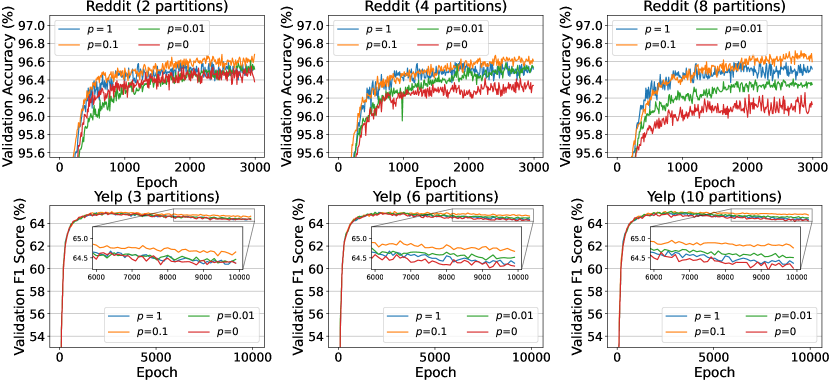
Figure 9: Convergence comparison between unsampled full-graph training (BNS-GCN with $p=1$), boundary-node sampled training ($0<p<1$), and isolated training ($p=0$) on Reddit and Yelp.

Appendix C Efficiency Comparison with Sampling-based Methods

Table 11 compares the training efficiency between the popular sampling-based methods and BNS-GCN under the same settings of the main content. As can be seen, BNS-GCN outperforms the sampling-based methods with a great margin, while achieving a higher accuracy (see Table 4 of the main content).

Table 11: Comparison of training efficiency on Reddit, where BNS-GCN with various boundary sampling rates under 8 partitions are shown.

Method	GraphSAGE	FastGCN	VR-GCN	ClusterGCN	BNS-GCN(1)	BNS-GCN(0.1)	BNS-GCN(0.01)
Train time per epoch	6.20s	5.08s	3.85s	1.35s	0.777s	0.198s	0.150s
Speedup	1$\times$	1.22$\times$	1.61$\times$	4.59$\times$	8.0$\times$	31.3$\times$	41.3$\times$

Appendix D Overhead of Boundary Node Sampling

In this section, we evaluate the overhead introduced by the boundary node sampling of BNS-GCN under different sampling rates and number of partitions, and also compare it with the overhead of the state-of-the-art sampling methods. Table 12 summarizes the results. We observe that node, edge, and random walk sampling can introduce a non-trivial overhead, which is up to 24% of training time (Zeng et al., 2020). By contrast, boundary node sampling incurs only a negligible overhead, i.e., 0%$\sim$7.3%, because it only needs to perform sampling on the boundary region instead of the whole graph as used in the state-of-the-art methods. Also, the light weightiness of boundary nodes sampling lies in its parallizability across partitions, instead of requiring sequential processing. Besides, we also compare BNS-GCN with the graph-level sampling method such as ClusterGCN (Chiang et al., 2019). We find that the overhead of boundary node sampling is still much lower than ClusterGCN, because ClusterGCN needs to merge multiple subgraphs into one cluster with a sampling time roughly proportional to the number of edges in the whole graph. By contrast, boundary node sampling only needs to modify those boundary edges of selected boundary nodes, and its sampling time is proportional only to the number of boundary edges, which is only a fraction of ClusterGCN.

Table 12: Comparison of BNS-GCN’s sampling overhead with the state-of-the-art methods in GraphSAINT (Zeng et al., 2020) on Reddit, where the overhead percentage is calculated by the sampling time divided by the training time.

The state-of-the-art samplers
Node	23%
Edge	20%
Random walk	24%
BNS-GCN sampler
# Partitions	2	4	8
$p=1.00$	0%
$p=0.10$	1.7%	3.2%	6.6%
$p=0.01$	1.3%	3.0%	7.3%
$p=0.00$	0%

Appendix E The Choice of $p$

In this section, we discuss how to choose the boundary node sampling rate $p$ in practice for maximizing the efficiency of GCN training. Empirically, $p=0.1$ combines the best of all worlds: throughput boosting, communication reduction, memory saving, convergence speedup, and final accuracy, as well as sampling overhead, across different number of partitions and different datasets, according to our extensive experiments. To further validate this, we compare the test accuracy of $p$ between 0.1 and 1 and summarize the results in Table 13. We can see that the advantage of $p=0.1$ still holds, i.e., offering similar accuracy but less communication/memory compared with higher $p$ values.

Table 13: Test accuracy of BNS-GCN with a sampling rate $p$ between 0.1 and 1.

Dataset	$p=0.1$	$p=0.3$	$p=0.5$	$p=0.8$	$p=1.0$
Reddit (2 partitions)	97.17%	97.18%	97.15%	97.13%	97.11%
ogbn-product (5 partitions)	79.36%	79.30%	79.34%	79.24%	79.14%

Appendix F Artifact Appendix

F.1 Abstract

Our artifact contains the full source code of BNS-GCN. It includes both the baseline (vanilla partition-parallel training) and the proposed boundary-node-sampled training for GCNs on various datasets. Running the code requires a machine (at least 120 GB host memory) with multiple (at least five) Nvidia GPUs (at least 11GB each). Software is provided with our docker image. With the aforementioned hardware and software, running our provided scripts will validate the main experiments in the paper, such as per-epoch training time, training time breakdown, memory usage, and accuracy.

F.2 Artifact check-list (meta-information)

• Algorithm: Graph Convolutional Network (GCN), Distributed Training, Random Sampling

• Data set: Reddit, ogbn-products, Yelp (all included in our docker or software setup)

• Run-time environment: Ubuntu 18.04, Python 3.8, CUDA 11.1, PyTorch 1.8.0, DGL 0.7.0, OGB 1.3.0

• Hardware: A X64-CPU machine with at least 120 GB host memory, at least five Nvidia GPUs (at least 11GB each).

• Execution: Bash scripts, Running each experiment takes less than 1 hour.

• Metrics: Training time, training time breakdown, memory usage, accuracies

• Output: Console, and log file

• How much disk space required (approximately)?: 50GB

• How much time is needed to prepare workflow (approximately)?: 30 minutes

• How much time is needed to complete experiments (approximately)?: 10 hours

• Publicly available?: yes

• Code licenses (if publicly available)?: MIT License

• Archived (provide DOI)?: 10.5281/zenodo.6079700

F.3 Description

F.3.1 How delivered

• Source code in the archival repository for ACM badges: https://doi.org/10.5281/zenodo.6079700.

• Latest source code in GitHub repository: https://github.com/RICE-EIC/BNS-GCN.

• Docker image: https://hub.docker.com/r/cheng1016/bns-gcn.

• Approximate disk space: 50GB, used for large datasets

F.3.2 Hardware dependencies

• A X86-CPU machine with at least 120 GB host memory

• At least five Nvidia GPUs (at least 11 GB each)

F.3.3 Software dependencies

All provided in our docker image:

• Ubuntu 18.04

• Python 3.8

• CUDA 11.1

• PyTorch 1.8.0

• customized DGL 0.7.0

• OGB 1.3.0

F.3.4 Data sets

All dataset (Reddit, ogbn-products, Yelp) are either included in our docker image or to be downloaded by our scripts.

F.4 Installation

Detailed instructions are provided in README.md in our GitHub repository. For example, just run docker pull cheng1016/bns-gcn followed by docker run --gpus all -it cheng1016/bns-gcn.

F.5 Experiment workflow

The workflow involves invoking top-level main.py which then drives other modules for distributed GCN training. All “one-click-to-run” scripts to reproduce main experiments in the paper are provided in the scripts/*.sh in our GitHub repository.

F.6 Evaluation and expected result

All steps are in scripts/*.sh in our GitHub repository.

F.7 Experiment customization

We provide a detailed guide for customization in README.md in our GitHub repository. Hyper-parameters and configurations can be customized by the options fed to main.py, e.g., allowing users to choose the number of training epochs, the number of graph partitions (or GPUs), different partitioning methods, and even extending training to multiple machines with multiple GPUs.

F.8 Notes

For the hyper-scale dataset ogbn-papers100M, the experiment was conducted on 32 machines, each of which has 6 Tesla V100 (16GB) with IBM Power9 (605GB).

References

- Buluç et al. (2016) Buluç, A., Meyerhenke, H., Safro, I., Sanders, P., and Schulz, C. Recent advances in graph partitioning. In Algorithm Engineering, pp. 117–158. Springer, 2016.
- Chen et al. (2018a) Chen, J., Ma, T., and Xiao, C. Fastgcn: fast learning with graph convolutional networks via importance sampling. arXiv preprint arXiv:1801.10247, 2018a.
- Chen et al. (2018b) Chen, J., Zhu, J., and Song, L. Stochastic training of graph convolutional networks with variance reduction. In International Conference on Machine Learning, pp. 942–950. PMLR, 2018b.
- Chen et al. (2020) Chen, M., Wei, Z., Ding, B., Li, Y., Yuan, Y., Du, X., and Wen, J.-R. Scalable graph neural networks via bidirectional propagation. Advances in Neural Information Processing Systems, 33, 2020.
- Chen et al. (2019) Chen, R., Shi, J., Chen, Y., Zang, B., Guan, H., and Chen, H. Powerlyra: Differentiated graph computation and partitioning on skewed graphs. ACM Transactions on Parallel Computing (TOPC), 5(3):1–39, 2019.
- Chiang et al. (2019) Chiang, W.-L., Liu, X., Si, S., Li, Y., Bengio, S., and Hsieh, C.-J. Cluster-gcn: An efficient algorithm for training deep and large graph convolutional networks. In Proceedings of the 25th ACM SIGKDD International Conference on Knowledge Discovery & Data Mining, pp. 257–266, 2019.
- Cong et al. (2020) Cong, W., Forsati, R., Kandemir, M., and Mahdavi, M. Minimal variance sampling with provable guarantees for fast training of graph neural networks. In Proceedings of the 26th ACM SIGKDD International Conference on Knowledge Discovery & Data Mining, pp. 1393–1403, 2020.
- Fey et al. (2021) Fey, M., Lenssen, J. E., Weichert, F., and Leskovec, J. Gnnautoscale: Scalable and expressive graph neural networks via historical embeddings. arXiv preprint arXiv:2106.05609, 2021.
- Gandhi & Iyer (2021) Gandhi, S. and Iyer, A. P. P3: Distributed deep graph learning at scale. In 15th USENIX Symposium on Operating Systems Design and Implementation (OSDI 21), pp. 551–568, 2021.
- Gonzalez et al. (2012) Gonzalez, J. E., Low, Y., Gu, H., Bickson, D., and Guestrin, C. Powergraph: Distributed graph-parallel computation on natural graphs. In Presented as part of the 10th USENIX Symposium on Operating Systems Design and Implementation (OSDI 12), pp. 17–30, 2012.
- Gower et al. (2019) Gower, R. M., Loizou, N., Qian, X., Sailanbayev, A., Shulgin, E., and Richtárik, P. Sgd: General analysis and improved rates. In International Conference on Machine Learning, pp. 5200–5209. PMLR, 2019.
- Hamilton et al. (2017) Hamilton, W., Ying, Z., and Leskovec, J. Inductive representation learning on large graphs. In Advances in neural information processing systems, pp. 1024–1034, 2017.
- Harlap et al. (2018) Harlap, A., Narayanan, D., Phanishayee, A., Seshadri, V., Devanur, N., Ganger, G., and Gibbons, P. Pipedream: Fast and efficient pipeline parallel dnn training. arXiv preprint arXiv:1806.03377, 2018.
- Hu et al. (2020) Hu, W., Fey, M., Zitnik, M., Dong, Y., Ren, H., Liu, B., Catasta, M., and Leskovec, J. Open graph benchmark: Datasets for machine learning on graphs. arXiv preprint arXiv:2005.00687, 2020.
- Huang et al. (2018) Huang, W., Zhang, T., Rong, Y., and Huang, J. Adaptive sampling towards fast graph representation learning. In Advances in neural information processing systems, pp. 4558–4567, 2018.
- Jia et al. (2020) Jia, Z., Lin, S., Gao, M., Zaharia, M., and Aiken, A. Improving the accuracy, scalability, and performance of graph neural networks with roc. Proceedings of Machine Learning and Systems (MLSys), pp. 187–198, 2020.
- Karypis & Kumar (1998) Karypis, G. and Kumar, V. A fast and high quality multilevel scheme for partitioning irregular graphs. SIAM Journal on scientific Computing, 20(1):359–392, 1998.
- Kipf & Welling (2016) Kipf, T. N. and Welling, M. Semi-supervised classification with graph convolutional networks. arXiv preprint arXiv:1609.02907, 2016.
- Krizhevsky (2014) Krizhevsky, A. One weird trick for parallelizing convolutional neural networks. arXiv preprint arXiv:1404.5997, 2014.
- Lerer et al. (2019) Lerer, A., Wu, L., Shen, J., Lacroix, T., Wehrstedt, L., Bose, A., and Peysakhovich, A. Pytorch-biggraph: A large-scale graph embedding system. arXiv preprint arXiv:1903.12287, 2019.
- Li et al. (2020) Li, S., Zhao, Y., Varma, R., Salpekar, O., Noordhuis, P., Li, T., Paszke, A., Smith, J., Vaughan, B., Damania, P., et al. Pytorch distributed: Experiences on accelerating data parallel training. arXiv preprint arXiv:2006.15704, 2020.
- Li et al. (2018a) Li, Y., Park, J., Alian, M., Yuan, Y., Qu, Z., Pan, P., Wang, R., Schwing, A. G., Esmaeilzadeh, H., and Kim, N. S. A network-centric hardware/algorithm co-design to accelerate distributed training of deep neural networks. In Proceedings of the 51st IEEE/ACM International Symposium on Microarchitecture (MICRO’18), Fukuoka City, Japan, October 2018a.
- Li et al. (2018b) Li, Y., Yu, M., Li, S., Avestimehr, S., Kim, N. S., and Schwing, A. Pipe-sgd: A decentralized pipelined sgd framework for distributed deep net training. In Proceedings of the 32nd Conference on Neural Information Processing Systems (NIPS’18), Montreal, Canada, December 2018b.
- Liu et al. (2022) Liu, Z., Zhou, K., Yang, F., Li, L., Chen, R., and Hu, X. EXACT: Scalable graph neural networks training via extreme activation compression. In International Conference on Learning Representations, 2022. URL https://openreview.net/forum?id=vkaMaq95_rX.
- Ma et al. (2019) Ma, L., Yang, Z., Miao, Y., Xue, J., Wu, M., Zhou, L., and Dai, Y. NeuGraph: Parallel deep neural network computation on large graphs. In 2019 USENIX Annual Technical Conference (USENIX ATC 19), pp. 443–458, 2019.
- Nguyen et al. (2013) Nguyen, D., Lenharth, A., and Pingali, K. A lightweight infrastructure for graph analytics. In Proceedings of the Twenty-Fourth ACM Symposium on Operating Systems Principles, pp. 456–471, 2013.
- Paszke et al. (2019) Paszke, A., Gross, S., Massa, F., Lerer, A., Bradbury, J., Chanan, G., Killeen, T., Lin, Z., Gimelshein, N., Antiga, L., et al. Pytorch: An imperative style, high-performance deep learning library. In Advances in neural information processing systems, pp. 8026–8037, 2019.
- Rong et al. (2019) Rong, Y., Huang, W., Xu, T., and Huang, J. Dropedge: Towards deep graph convolutional networks on node classification. In International Conference on Learning Representations, 2019.
- Shun & Blelloch (2013) Shun, J. and Blelloch, G. E. Ligra: a lightweight graph processing framework for shared memory. In Proceedings of the 18th ACM SIGPLAN symposium on Principles and practice of parallel programming, pp. 135–146, 2013.
- Thakur et al. (2005) Thakur, R., Rabenseifner, R., and Gropp, W. Optimization of collective communication operations in mpich. Int. J. High Perform. Comput. Appl., 19(1):49–66, February 2005.
- Thorpe et al. (2021) Thorpe, J., Qiao, Y., Eyolfson, J., Teng, S., Hu, G., Jia, Z., Wei, J., Vora, K., Netravali, R., Kim, M., et al. Dorylus: affordable, scalable, and accurate gnn training with distributed cpu servers and serverless threads. In 15th USENIX Symposium on Operating Systems Design and Implementation (OSDI 21), pp. 495–514, 2021.
- Tripathy et al. (2020) Tripathy, A., Yelick, K., and Buluc, A. Reducing communication in graph neural network training. arXiv preprint arXiv:2005.03300, 2020.
- Veličković et al. (2017) Veličković, P., Cucurull, G., Casanova, A., Romero, A., Lio, P., and Bengio, Y. Graph attention networks. arXiv preprint arXiv:1710.10903, 2017.
- Wan et al. (2022) Wan, C., Li, Y., Wolfe, C. R., Kyrillidis, A., Kim, N. S., and Lin, Y. PipeGCN: Efficient full-graph training of graph convolutional networks with pipelined feature communication. In International Conference on Learning Representations, 2022. URL https://openreview.net/forum?id=kSwqMH0zn1F.
- Wang et al. (2019) Wang, M., Zheng, D., Ye, Z., Gan, Q., Li, M., Song, X., Zhou, J., Ma, C., Yu, L., Gai, Y., Xiao, T., He, T., Karypis, G., Li, J., and Zhang, Z. Deep graph library: A graph-centric, highly-performant package for graph neural networks. arXiv preprint arXiv:1909.01315, 2019.
- with Code (2020) with Code, P. Node Classification on Reddit, sep 2020. URL https://paperswithcode.com/sota/node-classification-on-reddit.
- Xu et al. (2018) Xu, K., Hu, W., Leskovec, J., and Jegelka, S. How powerful are graph neural networks? arXiv preprint arXiv:1810.00826, 2018.
- Ying et al. (2018) Ying, R., He, R., Chen, K., Eksombatchai, P., Hamilton, W. L., and Leskovec, J. Graph convolutional neural networks for web-scale recommender systems. In Proceedings of the 24th ACM SIGKDD International Conference on Knowledge Discovery & Data Mining, pp. 974–983, 2018.
- Zeng et al. (2020) Zeng, H., Zhou, H., Srivastava, A., Kannan, R., and Prasanna, V. Graphsaint: Graph sampling based inductive learning method. arXiv preprint arXiv:1907.04931, 2020.
- Zhang & Chen (2018) Zhang, M. and Chen, Y. Link prediction based on graph neural networks. In Advances in Neural Information Processing Systems, pp. 5165–5175, 2018.
- Zheng et al. (2020) Zheng, D., Ma, C., Wang, M., Zhou, J., Su, Q., Song, X., Gan, Q., Zhang, Z., and Karypis, G. Distdgl: distributed graph neural network training for billion-scale graphs. In 2020 IEEE/ACM 10th Workshop on Irregular Applications: Architectures and Algorithms (IA3), pp. 36–44. IEEE, 2020.
- Zhu et al. (2019) Zhu, R., Zhao, K., Yang, H., Lin, W., Zhou, C., Ai, B., Li, Y., and Zhou, J. Aligraph: A comprehensive graph neural network platform. arXiv preprint arXiv:1902.08730, 2019.
- Zhu et al. (2016) Zhu, X., Chen, W., Zheng, W., and Ma, X. Gemini: A computation-centric distributed graph processing system. In 12th USENIX Symposium on Operating Systems Design and Implementation (OSDI 16), pp. 301–316, 2016.
- Zou et al. (2019) Zou, D., Hu, Z., Wang, Y., Jiang, S., Sun, Y., and Gu, Q. Layer-dependent importance sampling for training deep and large graph convolutional networks. In Advances in Neural Information Processing Systems, pp. 11249–11259, 2019.