What is a randomization test?

Abstract

The meaning of randomization tests has become obscure in statistics education and practice over the last century. This article makes a fresh attempt at rectifying this core concept of statistics. A new term—“quasi-randomization test”—is introduced to define significance tests based on theoretical models and distinguish these tests from the “randomization tests” based on the physical act of randomization. The practical importance of this distinction is illustrated through a real stepped-wedge cluster-randomized trial. Building on the recent literature on randomization inference, a general framework of conditional randomization tests is developed and some practical methods to construct conditioning events are given. The proposed terminology and framework are then applied to understand several widely used (quasi-)randomization tests, including Fisher’s exact test, permutation tests for treatment effect, quasi-randomization tests for independence and conditional independence, adaptive randomization, and conformal prediction.

Keywords: Causal Inference; Cluster randomized trial; Conditioning; Permutation tests; Quasi-experiment.

1 Introduction

Randomization is one of the oldest and most important ideas in statistics, playing several roles in experimental designs and inference (Cox, 2009). Randomization tests were introduced by Fisher (1935, Chapter 21) to substitute Student’s $t$-tests when normality does not hold, and to restore randomization as “the physical basis of the validity of statistical tests”. This idea was immediately extended by Pitman (1937), Welch (1937), Wilcoxon (1945), Kempthorne (1952), and many others.

An appealing property of randomization tests is that they have exact control of the nominal type I error rate in finite samples without relying on any distributional assumptions. This is particularly attractive in modern statistical applications that involve arbitrarily complex sampling distributions. Recently, there has been a rejuvenated interest in randomization tests in several areas of statistics, including testing associations in genomics (Bates et al., 2020; Efron et al., 2001), testing conditional independence (Candès et al., 2018; Berrett et al., 2020), conformal inference for machine learning methods (Lei et al., 2013; Vovk et al., 2005), analysis of complex experimental designs (Ji et al., 2017; Morgan and Rubin, 2012), evidence factors for observational studies (Karmakar et al., 2019; Rosenbaum, 2010, 2017), and causal inference with interference (Athey et al., 2018; Basse et al., 2019).

Along with its popularity, the term “randomization test” is increasingly used in statistics and its applications, but unfortunately often not to represent what it means originally. For example, at the time of writing Wikipedia redirects “randomization test” to a page titled “Resampling (statistics)” and describes it alongside bootstrapping, jackknifing, and subsampling. The terms “randomization test” and “permutation test” are often used interchangeably, which causes a great deal of confusion. A common belief is that randomization tests rely on certain kinds of group structure or exchangeability (Lehmann and Romano, 2006; Southworth et al., 2009; Rosenbaum, 2017). This led some authors to categorize randomization tests as a special case of “permutation tests” (Ernst, 2004) or vice versa (Lehmann and Romano, 2006, p. 632). Furthermore, some authors started to use new and, in our opinion, redundant terminology. An example is “rerandomization test” (Brillinger et al., 1978; Gabriel and Hall, 1983), which is nothing more than an usual randomization test and confuses with a technique called “rerandomization” that is useful for improving covariate balance (Morgan and Rubin, 2012). For a historical clarification on the terminology, we refer the readers to Onghena (2017).

The main objective of this paper is to give a clear-cut formulation of the randomization test, so it can be distinguished from closely related concepts. Our formulation follows from the work of Rubin (1980), Rosenbaum (2002), Basse et al. (2019), and many others in causal inference based on the potential outcomes model first conceived by Neyman (1923). In fact, this was also the model adopted in the first line of works on the randomization tests by Pitman (1937), Welch (1937), and Kempthorne (1952). However, as the fields of survey sampling and experimental design grew apart since the 1930s, and because randomization tests often take simpler forms under the convenient exchangeability assumption, the popularity of the potential outcomes model had dwindled until Rubin (1974) introduced it to observational studies. In consequence, most contemporary statisticians are not familiar with this approach that can give a more precise characterization of randomization test and distinguish it from related ideas. Our discussion below will focus on the conceptual differences and key statistical ideas; detailed implementations and examples of randomization tests (and related tests) can be found in the references in this article and the book by Edgington and Onghena (2007).

1.1 Randomization tests vs. Permutation tests

Many authors have repeatedly pointed out that randomization tests and permutation tests are based on different assumptions and the distinguishing these terms is crucial. On one hand, randomization tests are based on “experimental randomization” (Kempthorne and Doerfler, 1969; Rosenberger et al., 2018), “random assignment” (Onghena, 2017), or the so-called “randomization model” (Ernst, 2004; Lehmann, 1975). On the other hand, permutation tests are based on “random sampling” (Kempthorne and Doerfler, 1969; Onghena, 2017), the so-called “population model” (Ernst, 2004; Lehmann, 1975; Rosenberger et al., 2018), or certain algebraic group structures (Lehmann and Romano, 2006; Southworth et al., 2009; Hemerik and Goeman, 2020). Moreover, unlike permutation tests, the validity of randomization tests is not based on the exchangeability assumption (Kempthorne and Doerfler, 1969; Onghena, 2017; Rosenberger et al., 2018; Hemerik and Goeman, 2020). Despite these suggestions, randomization test and permutation test are seldomly distinguished in practice.

The fundamental reason behind this confusing nomenclature is that a randomization test coincides with a permutation test in the simplest example where half of the experimental units are randomized to treatment and half to control. The coincidence is caused by the fact that all permutations of the treatment assignment are equally likely to realize in the assignment distribution. As this is usually the first example in a lecture or article where randomization tests or permutation tests are introduced, it is understandable that many think the basic ideas behind the two tests are the same.

The reconciliation, we believe, lies precisely in the names of these tests. Randomization refers to a physical action that makes the treatment assignment random, while permutation refers to a step of an algorithm that computes the significance level of a test. The former emphasizes the basis of inference, while the latter emphasizes the algorithmic side of inference, so neither “randomization test” or “permutation test” subsumes the other. In the example above, we can use either term to refer to the same test, but the name “randomization test” is preferable as it provides more information about the context of the problem.

1.2 Randomization tests vs. Quasi-randomization tests

To further clarify the distinction between randomization tests and permuation tests, we believe it is helpful to introduce a new term—“quasi-randomization tests”. It refers to any test that is not based on the physical act of randomization. It is exactly the complement of randomization tests. A test can then be characterized in two dimensions: (1) whether it is based on the physical act of randomization; and (2) how it is computed (using permutations, resampling, or distributional models). With this in mind, we can now distinguish two tests that are computationally identical (in the sense that the same acceptance/rejection decision is always reached given the same observed data) based on their underlying assumptions.

To illustrate this, consider permutation test in the following two scenarios. In the first scenario, an even number of units are paired before being randomized to receive one of two treatments, with exactly one unit in each pair receiving each treatment. In the second scenario, the units are observed (but not randomized) and we pair each unit receiving the first treatment with a different unit receiving the second treatment. To test the null hypothesis that the two treatments have no difference on any unit, we can permute treatment assignments within the pairs. Although these tests are computationally identical, the same conclusion (e.g. rejecting the null hypothesis) from them may carry very different weight. The second test relies on the assumption that the two units in the same pair are indeed exchangeable besides their treatment status. This assumption can be easily violated if the units are different in some way; even if they look comparable in every way we can think of now, someone in the future may discover an overlooked distinction. Randomization plays a crucial role in hedging against such a possibility (Kempthorne and Doerfler, 1969; Marks, 2003). In the new terminology we propose, both tests are permutation tests, but the first is a randomization test and the second is a quasi-randomization test. That is, even if a randomization test and a quasi-randomization test are algorithmically identical, they have entirely different inferential basis and thus must be distinguished.

The distinction between a randomization test and a quasi-randomization test is intimately related to causal inference using experimental and observational data. Our nomenclature is motivated by term “quasi-experiment” coined by Campbell and Stanley (1963) to refer to an observational study that is designed to estimate the causal impact of an intervention. Since then, this term has been widely used in social science (Cook et al., 2002).

1.3 Randomness used in a randomization test

At this point, our answer to the question in the title of this article should already be clear. A randomization test is precisely what its name suggests—a hypothesis test based on randomization and nothing more than randomization. But what does “based on randomization” exactly mean? To answer this question, it is helpful to consider counterfactual versions of the data. In the causal inference literature, this is known as the Neyman-Rubin model (Holland, 1986), which postulates the existence of a potential outcome (or counterfactual) for every possible realization of the treatment assignment. Broadly speaking, a “treatment assignment” can be anything that is randomized in an experiment (so not an actual treatment), while the “outcome” includes everything observed after randomization. To clarify the nature of randomization tests, we separate the randomness in data and statistical tests into

1. Randomness introduced by the nature in the potential outcomes;

2. Randomness introduced by the experimenter (e.g., drawing balls from an urn);

3. Randomness introduced by the analyst, which is optional.

Using this trichotomy, a randomization test can be understood as a hypothesis test that conditions on the potential outcomes and obtains the sampling distribution (often called the randomization distribution) using the second and third sources of randomness. A randomization test is based solely on the randomness introduced by humans (experimenters and/or analysts), thereby providing a coherent logic of scientific induction (Fisher, 1956).

We would like to make two comments on the definitions above. First, the notion of potential outcomes, first introduced by Neyman in the context of randomized agricultural experiments, was not uncommon in the description of randomization tests. This was often implicit, but the seminal paper by Welch (1937) used potential outcomes to clarify that randomization test is applicable to Fisher’s sharp null rather than Neyman’s null concerning the average treatment effect. Second, the difference between randomization before and after an experiment is also well recognized (Basu, 1980; Kempthorne and Doerfler, 1969).

Much of the recent literature on randomization tests is motivated by the interference (cross-unit effect) problem in causal inference. A key feature of the interference problem is that the null hypothesis is only “partially sharp”, another term we coin in this article to refer to the phenomenon that the potential outcomes are not always imputable under all possible treatment assignments. In consequence, a randomization test that uses all the randomness introduced by the experimenter may be uncomputable. A general solution to this problem is conditioning on some carefully constructed events of the treatment assignment.

1.4 An overview of the article

Section 2 investigates a real cluster-randomized controlled trial using (quasi-)randomization tests that are based on different assumptions about the data. Section 3 develops an overarching theory for (conditional) randomization tests by generalizing the classical Neyman-Rubin causal model. The usage of the potential outcome notation allows us to give a precise definition of randomization test. Section 4 then reviews some practical methods to construct conditional randomization tests. Section 5 discusses some quasi-randomization tests in the recent literature, including tests for (conditional) independence and conformal prediction. Finally, Section 6 concludes the paper with some further discussion.

Notation. We use calligraphic letters for sets, boldface letters for vectors, upper-case letters for random quantities, and lower-case letters for fixed quantities. We use a single integer in a pair of square brackets as a shorthand notation for the indexing set from $1$: $[N]=\{1,\dotsc,N\}$. We use set-valued subscript to denote a sub-vector; for example, $\bm{Y}_{\{2,4,6\}}=(Y_{2},Y_{4},Y_{6})$. We use $X\mathchoice{\mathrel{\hbox to0.0pt{$\displaystyle\perp$\hss}\mkern 2.0mu{\displaystyle\perp}}}{\mathrel{\hbox to0.0pt{$\textstyle\perp$\hss}\mkern 2.0mu{\textstyle\perp}}}{\mathrel{\hbox to0.0pt{$\scriptstyle\perp$\hss}\mkern 2.0mu{\scriptstyle\perp}}}{\mathrel{\hbox to0.0pt{$\scriptscriptstyle\perp$\hss}\mkern 2.0mu{\scriptscriptstyle\perp}}}Y$ to represent the random variable $X$ is independent of the random variable $Y$.

2 An illustrative example: The Australia weekend health services disinvestment trial

We first illustrate the conceptual and practical differences of randomization and quasi-randomization tests through a real data example.

2.1 Trial background

Haines et al. (2017) reported the results of a cluster randomized controlled trial about the impact of disinvestment from weekend allied health services across acute medical and surgical wards. The trial consisted of two phases—in the first phase, the original weekend allied health service model was terminated, and in the second phase, a newly developed model was instated. The trial involved 12 hospital wards in 2 hospitals in Melbourne, Australia. As our main purpose is to demonstrate the distinction between randomization and quasi-randomisation tests, we will focus on the first phase of the trial and 6 wards in the Dandenong Hospital. The original article investigated a number of patient outcomes; below we will just focus on patient length of stay after a log transformation.

A somewhat unusual feature of the design of this trial is that the hospital wards received treatment (no weekend health services) in a staggered fashion. This is often referred to as the “stepped-wedge” design. In the first month of the trial period, all 6 wards received regular weekend health service. In each of the following 6 months, one ward crossed over to the treatment, and the order was randomized at the beginning of the trial. The dataset contains patient-level information including when and where they were hospitalized, their length of stay, and other demographic and medical information. More details about the data can be found in the trial report (Haines et al., 2017). Figure 1 illustrates the stepped-wedge design and shows the mean outcome of each ward in each calendar month; the average (log-transformed) length of stay tends to be higher after the treatment, but more careful analysis is required to decide if such a pattern is statistically meaningful in some way.

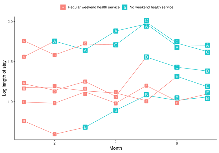
Figure 1: Australia weekend health services disinvestment trial: a 7-month stepped-wedge design with monthly ward-level mean outcomes. The six hospital wards are indexed by A,B,C,D,E and F.

2.2 Trial analysis via (quasi-)randomization tests

We say a patient is exposed to the treatment if there is no weekend health services when the patient was admitted to a hospital ward. The exposure status is jointly determined by the actual treatment (crossover order of the wards) and when and where the patient was admitted. This motivates seven permutation tests for the sharp null hypothesis that removing the weekend allied health services has no effect on the length of stay. These tests differ in which variable(s) they permuted. In particular, we considered permuting

1. Crossover: the crossover order of the hospital wards to be exposed to the treatment;

2. Time: calendar months during which the patients visited the hospital;

3. Ward: hospital wards visited by the patient.

As the trial only randomizes the crossover order, only the test permuting crossover qualifies as a randomization test according to our definition in the Introduction. All six other tests that involve permuting other variables are instances of quasi-randomization tests in our terminology because their permuted variables are not randomized in the trial. The quasi-randomization tests may have smaller p-values than the randomization test, but their validity requires the exchangeability assumption which may not hold. For instance, it is questionable to permute the admission times if the patients have seasonal diseases or permute the hospital wards if the wards have different specialties (which is indeed the case in this trial).

We considered three test statistics for the permutation tests. The first statistic $T_{1}$ is simply the exposed-minus-control difference in the mean outcome; equivalently, this can be obtained by the least-squares estimator for a simple linear regression of log length of stay on exposure status (with intercept). The second statistic $T_{2}$ is the estimated coefficient of the exposure status in the linear regression that adjusts for the hospital wards, and the third statistic $T_{3}$ further adjusts for the time of hospitalization (in calendar month).

Table 1: Results of (quasi-)randomization tests applied to the Australia weekend health services disinvestment trial. $T_{1}$ is the exposed-minus-control difference of log length of stay. $T_{2}$ is the coefficient of exposure status in the linear regression of log length of stay on treatment status and hospital ward. $T_{3}$ is the coefficient of exposure status in the linear regression of log length of stay on exposure status, hospital ward, and time of hospitalization. Results of the permutation tests are compared with the output of the corresponding linear models assuming normal homoskedastic noise. (CI: 90% Confidence Interval.)

	$T_{1}$ (adjust for nothing)		$T_{2}$ (adjust for ward)		$T_{3}$ (adjust for ward & time)
	p-value	CI	p-value	CI	p-value	CI
Randomization test	$0.0833$	[-0.09, 0.72]	$0.0042$	[0.06, 0.3]	$0.0069$	[0.06, 0.31]
Quasi-Randomization tests
Time	$0.0000$	[0.13, 0.24]	$0.0000$	[0.11, 0.21]	$0.0000$	[0.09, 0.23]
Ward	$0.0000$	[0.30, 0.42]	$0.0049$	[0.04, 0.19]	$0.0000$	[0.10, 0.25]
Time & ward	$0.0000$	[0.25, 0.33]	$0.0000$	[0.11, 0.22]	$0.0000$	[0.09, 0.23]
Crossover & time	$0.0029$	[0.08, 0.47]	$0.0000$	[0.12, 0.21]	$0.0000$	[0.09, 0.23]
Crossover & ward	$0.0000$	[0.29, 0.41]	$0.0093$	[0.02, 0.18]	$0.0001$	[0.08, 0.24]
Crossover, time & ward	$0.0000$	[0.24, 0.33]	$0.0000$	[0.11, 0.21]	$0.0001$	[0.09, 0.23]
Linear model	$0.0000$	[0.24, 0.34]	$0.0000$	[0.11, 0.22]	$0.0001$	[0.08, 0.24]

2.3 Results: Randomization test v.s. Quasi-randomization tests

Table 1 shows the one-sided p-values (alternative hypothesis is positive treatment effect) of the seven permutation tests with these three statistics. Confidence intervals were obtained by inverting the two one-sided permutation tests of null hypotheses with varying constant treatment effects (see Section 3.2 for more details). Results are further compared with the corresponding output of the two linear models assuming normal homoskedastic noise. It may be useful to know that the adjusted $R^{2}$ of the first linear model is only 1.8%, while the adjusted $R^{2}$ of the second and third models are both about 8.4%.

The randomization test that only permutes the crossover order almost always gave the largest $p$-value and widest confidence intervals. This is perhaps not too surprising given that there are only $6!=720$ permutations in total and thus the smallest possible permutation p-value is $1/720\approx 0.0014$. Using better statistics ($T_{2}$ or $T_{3}$) substantially reduces the length of the confidence intervals. On the other hand, the quasi-randomization tests, while generally giving smaller $p$-values, were quite sensitive to the choice of the test statistic. In particular, the four quasi-randomization tests that permute ward (and other variables) produced non-overlapping confidence intervals with $T_{1}$ and $T_{2}$. The same phenomenon also occurs with the normal linear model (last row of the table).

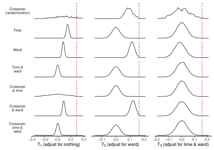
Figure 2: Australia weekend health services disinvestment trial: (quasi-)randomization distributions of three different test statistics.

To better understand the difference between randomization and quasi-randomization tests, Figure 2 shows the randomization distributions of $T_{1}$, $T_{2}$, and $T_{3}$ when different variables are permuted. The quasi-randomization distributions are approximated by Monte Carlo simulation and the kernel density estimator. Each red dash line in the figure indicates the test statistics on the observed data without any permutation. Each p-value in Table 1 is calculated by computing the corresponding area of the (quasi)-randomization distribution—the black curve—above the observed statistic—the dashed red line. A small p-value means that the observed test statistics is more extreme than the test statistics on the permuted data for most of the permutations considered, which is a strong evidence of a positive treatment effect on the log length of stay conjectured in Figure 1.

Notably, in the top row of Figure 2, the randomization distribution of $T_{1}$ is quite flat, indicating low power. In contrast, the distributions of $T_{2}$ and $T_{3}$ have sharper peaks. Interestingly, the randomization distribution of $T_{2}$ (adjusted for ward) is clearly not centred at $0$. This is due to a general upward trend in the length of stay over the course of this trial as shown in Figure 1. Since the wards gradually crossed over to the treatment group, this trend confounds the causal effect under investigation. Thus, when the crossover order and/or hospital ward are permuted, the exposure status would have a positive coefficient in the linear model that does not adjust for time.

In the other rows of Figure 2, the distributions of $T_{1}$ and $T_{2}$ are centred at different places depending on which variables are permuted. This explains why inverting the quasi-randomization tests based on $T_{1}$ and $T_{2}$ gives non-overlapping confidence intervals in Table 1. Because $T_{3}$ adjusts both time and ward, its permutation distributions are much less affected by permuting time and ward, so the result of the quasi-randomization tests is very close to the randomization test (top row in that column) which only permutes the crossover order.

2.4 Recap

The real data example gives a clear demonstration of how a permutation test on the randomness it tries to exploit. The distinction between the randomization and (quasi-)randomization tests lead to practically different conclusions. Using a randomization test protects against model misspecification and allows us to take advantage of a better model safely in the test statistics without sacrificing validity or marking additional assumption. In contrast, quasi-randomization tests and tests based on the normal linear model are sensitive to model specification and tend to overstate statistical significance.

3 A general theory for randomization tests

Next, we provide a general framework of (conditional) randomization tests by formalizing and generalizing what has become a “folklore” in causal inference after the strong advocation by Rubin (1980) and Rosenbaum (2002). Many quasi-randomization tests in the literature (such as independence testing and conformal prediction) do not test a causal hypothesis but still fall within our framework by conceiving imaginary randomization (e.g. through an i.i.d. or exchangeability assumption). Importantly, it is often helpful to construct artificial “potential outcomes” in those problems to fully understand the underlying assumption; see Section 5 for some examples.

3.1 Potential outcomes and randomization

Consider an experiment on $N$ units in which a treatment variable $\bm{Z}\in\mathcal{Z}$ is randomized. We use boldface $\bm{Z}$ to emphasize that the treatment $\bm{Z}$ is usually multivariate. Most experiments assume that $\bm{Z}=(Z_{1},\dotsc,Z_{N})$ collects a common attribute of the experimental units (e.g., whether a drug is administered). However, this is not always the case and the dimension of the treatment variable $\bm{Z}$ is not important in the general theory. For example, in the Australia weekend health services disinvestment trial in Section 2, the treatment $\bm{Z}$ (crossover order) is randomized at the ward level, while the patient level outcomes (length of stay). So $\mathcal{Z}$ has $6!=720$ permutations of the wards. What the theory below requires is that (i) $\bm{Z}$ is randomized in an exogenous way by the experimenter; random number generator) (ii) the distribution of $\bm{Z}$ is known (often called the treatment assignment mechanism); and (iii) one can reasonably define or conceptualize the potential outcomes of the experimental units under different treatment assignments.

To formalize these requirements, we adopt the potential outcome (also called the Neyman-Rubin or counterfactual) framework for causal inference (Holland, 1986; Neyman, 1923; Rubin, 1974). In this framework, unit $i$ has a vector of real-valued potential outcomes (or counterfactual outcomes) $(Y_{i}(\bm{z})\mid\bm{z}\in\mathcal{Z})$. We assume the observed outcome (or factual outcome) for unit $i$ is given by $Y_{i}=Y_{i}(\bm{Z})$, where $\bm{Z}$ is the realized treatment assignment. This is often referred to as the consistency assumption in the causal inference literature. In our running example, $Y_{i}(\bm{z})$ is the (potential) length of stay of patient $i$ had the crossover order of the wards been $\bm{z}$. When the treatment $\bm{Z}$ is an $N$-vector, the no interference assumption is often invoked to reduce the number of potential outcomes; this essentially says that $Y_{i}(\bm{z})$ only depends on $\bm{z}$ through $z_{i}$. However, our theory does not rely on this assumption but treats it as part of the sharp null hypothesis introduced below.

It is convenient to introduce some vector notation for the potential and realized outcomes. Let $\bm{Y}(\bm{z})=(Y_{1}(\bm{z}),\dotsc,Y_{N}(\bm{z}))\in\mathcal{Y}\subseteq\mathbb{R}^{N}$ and $\bm{Y}=(Y_{1},\dotsc,Y_{N})\in\mathcal{Y}$. Furthermore, let $\bm{W}=(\bm{Y}(\bm{z}):\bm{z}\in\mathcal{Z})\in\mathcal{W}$ collect all the potential outcomes (which are random variables defined on the same probability space as $\bm{Z}$). We will call $\bm{W}$ the potential outcomes schedule, following the terminology in Freedman (2009). This is also known as the science table in the literature (Rubin, 2005). It may be helpful to view potential outcomes $\bm{Y}(\bm{z})$ as a (vector-valued) function from $\mathcal{Z}$ to $\mathcal{Y}$; in this sense, $\mathcal{W}$ consists of all functions from $\mathcal{Z}$ to $\mathcal{Y}$.

Using this notation, The following assumption formally defines a randomized experiment.

Assumption 1 (Randomized experiment).

$\bm{Z}\mathchoice{\mathrel{\hbox to0.0pt{$\displaystyle\perp$\hss}\mkern 2.0mu{\displaystyle\perp}}}{\mathrel{\hbox to0.0pt{$\textstyle\perp$\hss}\mkern 2.0mu{\textstyle\perp}}}{\mathrel{\hbox to0.0pt{$\scriptstyle\perp$\hss}\mkern 2.0mu{\scriptstyle\perp}}}{\mathrel{\hbox to0.0pt{$\scriptscriptstyle\perp$\hss}\mkern 2.0mu{\scriptscriptstyle\perp}}}\bm{W}$ and the density function $\pi(\cdot)$ of $\bm{Z}$ (with respect to some reference measure on $\mathcal{Z}$) is known and positive everywhere.

We write the conditional distribution of $\bm{Z}$ given $\bm{W}$ in Assumption 1 as $\bm{Z}\mid\bm{W}\sim\pi(\cdot)$. This assumption formalizes the requirement that $\bm{Z}$ is randomized in an exogenous way. Intuitively, the potential outcomes schedule $\bm{W}$ is determined by the nature of experimental units. Since $\bm{Z}$ is randomized by the experimenter, it is reasonable to assume that $\bm{Z}\mathchoice{\mathrel{\hbox to0.0pt{$\displaystyle\perp$\hss}\mkern 2.0mu{\displaystyle\perp}}}{\mathrel{\hbox to0.0pt{$\textstyle\perp$\hss}\mkern 2.0mu{\textstyle\perp}}}{\mathrel{\hbox to0.0pt{$\scriptstyle\perp$\hss}\mkern 2.0mu{\scriptstyle\perp}}}{\mathrel{\hbox to0.0pt{$\scriptscriptstyle\perp$\hss}\mkern 2.0mu{\scriptscriptstyle\perp}}}\bm{W}$. In many experiments, the treatment is randomized according to some other observed covariates $\bm{X}$ (e.g., characteristics of the units or some observed network structure on the units). This can be dealt with by assuming $\bm{Z}\mathchoice{\mathrel{\hbox to0.0pt{$\displaystyle\perp$\hss}\mkern 2.0mu{\displaystyle\perp}}}{\mathrel{\hbox to0.0pt{$\textstyle\perp$\hss}\mkern 2.0mu{\textstyle\perp}}}{\mathrel{\hbox to0.0pt{$\scriptstyle\perp$\hss}\mkern 2.0mu{\scriptstyle\perp}}}{\mathrel{\hbox to0.0pt{$\scriptscriptstyle\perp$\hss}\mkern 2.0mu{\scriptscriptstyle\perp}}}\bm{W}\mid\bm{X}$ in Assumption 1 instead. Notice that in this case the treatment assignment mechanism $\pi$ may depend on $\bm{X}$. But to simplify the exposition, unless otherwise mentioned we will simply treat $\bm{X}$ as fixed, so $\bm{Z}\mathchoice{\mathrel{\hbox to0.0pt{$\displaystyle\perp$\hss}\mkern 2.0mu{\displaystyle\perp}}}{\mathrel{\hbox to0.0pt{$\textstyle\perp$\hss}\mkern 2.0mu{\textstyle\perp}}}{\mathrel{\hbox to0.0pt{$\scriptstyle\perp$\hss}\mkern 2.0mu{\scriptstyle\perp}}}{\mathrel{\hbox to0.0pt{$\scriptscriptstyle\perp$\hss}\mkern 2.0mu{\scriptscriptstyle\perp}}}\bm{W}$ is still true (in the conditional probability space with $\bm{X}$ fixed at the observed value).

For the rest of this article, we will assume $\bm{Z}$ is discrete so $\mathcal{Z}$ (e.g., $\mathcal{Z}=\{0,1\}^{N}$) is finite.

3.2 Partially sharp null hypotheses

As Holland (1986) pointed out, the fundamental problem in causal inference is that only one potential outcome can be observed for each unit under the consistency assumption. To overcome this problem, additional assumptions on $\bm{W}$ beyond randomization (Assumption 1) must be placed. In randomization inference, the required additional assumptions are (partially) sharp null hypotheses that relate different potential outcomes.

A typical (partially) sharp null hypothesis assumes that certain potential outcomes are equal or related in certain ways. As a concrete example, the no interference assumption assumes that $Y_{i}(\bm{z})=Y_{i}(\bm{z}^{*})$ whenever $z_{i}=z_{i}^{*}$. This allows one to simplify the notation $Y_{i}(\bm{z})$ as $Y_{i}(z_{i})$. The no treatment effect hypothesis (often referred to as Fisher’s sharp or exact null hypothesis) further assumes that $Y_{i}(z_{i})=Y_{i}(z_{i}^{*})$ for all $i$ and $z_{i},z_{i}^{*}$. When the treatment of each unit is binary (i.e., $Z_{i}$ is either $0$ or $1$), under the no interference assumption we may also consider the null hypothesis that the treatment effect is equal to a constant $\tau$, that is, $H_{0}:Y_{i}(1)-Y_{i}(0)=\tau$ for all $i$. Under the consistency assumption, this allows us to impute the potential outcomes as $Y_{i}(z_{i})=Y_{i}+(z_{i}-Z_{i})\tau$ for $z_{i}=0,1$.

More abstractly, a (partially) sharp null hypothesis $H$ defines a number of relationships between the potential outcomes. Each relationship allows us to impute some of the potential outcomes if another potential outcome is observed (through consistency). We can summarize these relationships using a set-valued mapping:

Definition 1.

A partially sharp null hypothesis defines an imputability mapping $\mathcal{H}:\leavevmode\nobreak\ \mathcal{Z}\times\mathcal{Z}\to 2^{[N]},(\bm{z},\bm{z}^{*})\mapsto\mathcal{H}(\bm{z},\bm{z}^{*}),$ where $\mathcal{H}(\bm{z},\bm{z}^{*})$ is the largest subset of $[N]$ such that $\bm{Y}_{\mathcal{H}(\bm{z},\bm{z}^{*})}(\bm{z}^{*})$ is imputable from $\bm{Y}(\bm{z})$ under $H$.

If we assume no interference and no treatment effect, all the potential outcomes are observed or imputable regardless of the realized treatment assignment $\bm{z}$, so $\mathcal{H}(\bm{z},\bm{z}^{*})=[N]$. In this case, we call $H$ a fully sharp null hypothesis. In more sophisticated problems, $\mathcal{H}(\bm{z},\bm{z}^{*})$ may depend on $\bm{z}$ and $\bm{z}^{*}$ in a nontrivial way and we call such hypothesis partially sharp. The concept of imputability has appeared before in Basse et al. (2019) and Puelz et al. (2019), though imputability was tied to test statistics under a hypothesis (see Definition 4 below) instead of the hypothesis itself.

In the Australia trial example (Section 2), we made an implicit “no interference” type assumption when obtaining the confidence intervals—we assumed that $Y_{i}(\bm{z})$ only depends on the implied binary exposure status $D_{i}(\bm{z})$ of the $i$th patient by the crossover order $\bm{z}$. That is, given when and where a patient is admitted, the patient’s potential outcome only depends on whether that ward has already crossed over to the treatment group according to $\bm{z}$. This would be violated when there is interference between the wards or the effect of ending the weekend health services is time-varying. This assumption allows us to abbreviate $Y_{i}(\bm{z})$ as $Y_{i}(D_{i}(\bm{z}))$ and impute the potential outcome $Y_{i}(0)$ under $H_{0}:Y_{i}(1)-Y_{i}(0)=\tau$. In the permutation tests, test statistics were computed using the three linear models in Section 2 with the shifted outcomes $Y_{i}-D_{i}(\bm{Z})\tau,\leavevmode\nobreak\ i=1,\dotsc,N$. The permutation tests were subsequently inverted to obtain confidence intervals of $\tau$.

3.3 Conditional randomization tests (CRTs)

To test a (partially) sharp null hypothesis, a randomization test compares an observed test statistic with its randomization distribution, which is given by the value of the statistic under a random treatment assignment. However, it may be impossible to compute the entire randomization distribution when some potential outcomes are not imputable (i.e. when $\mathcal{H}(\bm{z},\bm{z}^{*})$ is smaller than $[N]$). To tackle this issue, we confine ourselves to a smaller set of treatment assignments. This is formalized in the next definition.

Definition 2.

A conditional randomization test (CRT) for a treatment $\bm{Z}$ is defined by (i) A partition $\mathcal{R}=\{\mathcal{S}_{m}\}_{m=1}^{M}$ of $\mathcal{Z}$ such that $\mathcal{S}_{1},\dotsc,\mathcal{S}_{M}$ are disjoint subsets of $\mathcal{Z}$ satisfying $\mathcal{Z}=\bigcup_{m=1}^{M}\mathcal{S}_{m}$; and (ii) A collection of test statistics $(T_{m}(\cdot,\cdot))_{m=1}^{M}$, where $T_{m}:\mathcal{Z}\times\mathcal{W}\to\mathbb{R}$ is a real-valued function that computes a test statistic for each realization of the treatment assignment $\bm{Z}$ given the potential outcomes schedule $\bm{W}$.

Methods to construct $\mathcal{R}$ and examples will be discussed in the following sections.

Any partition $\mathcal{R}$ defines an equivalent relation $\equiv_{\mathcal{R}}$ and vice versa, so $\mathcal{S}_{1},\dotsc,\mathcal{S}_{M}$ are simply the equivalence classes generated by $\equiv_{\mathcal{R}}$. With an abuse of notation, we let $\mathcal{S}_{\bm{z}}\in\mathcal{R}$ denote the equivalence class containing $\bm{z}$. For any $\bm{z}\in\mathcal{S}_{m}$, we thus have $\mathcal{S}_{\bm{z}}=\mathcal{S}_{m}$ and $T_{\bm{z}}(\cdot,\cdot)=T_{m}(\cdot,\cdot)$. This notation is convenient because the p-value of the CRT defined below conditions on $\bm{Z}^{*}\in\mathcal{S}_{\bm{z}}$ when we observe $\bm{Z}=\bm{z}$. The following property follows immediately from the fact that $\equiv_{\mathcal{R}}$ is an equivalence relation:

Lemma 1 (Invariance of conditioning sets and test statistics).

For any $\bm{z}\in\mathcal{Z}$ and $\bm{z}^{*}\in\mathcal{S}_{\bm{z}}$, we have $\bm{z}\in\mathcal{S}_{\bm{z}}$, $\mathcal{S}_{\bm{z}^{*}}=\mathcal{S}_{\bm{z}}$ and $T_{\bm{z}^{*}}(\cdot,\cdot)=T_{\bm{z}}(\cdot,\cdot)$.

Definition 3.

The p-value of the CRT in Definition 2 is given by

$$P(\bm{Z},\bm{W})=\mathbb{P}^{*}\{T_{\bm{Z}}(\bm{Z}^{*},\bm{W})\leq T_{\bm{Z}}(\bm{Z},\bm{W})\mid\bm{Z}^{*}\in\mathcal{S}_{\bm{Z}},\bm{Z},\bm{W}\},$$ (1)

where $\bm{Z}^{*}$ is an independent copy of $\bm{Z}$ conditional on $\bm{W}$ and the notation $\mathbb{P}^{*}$ is used to emphasize that the probability is taken over $\bm{Z}^{*}$.

Because $\bm{Z}\mathchoice{\mathrel{\hbox to0.0pt{$\displaystyle\perp$\hss}\mkern 2.0mu{\displaystyle\perp}}}{\mathrel{\hbox to0.0pt{$\textstyle\perp$\hss}\mkern 2.0mu{\textstyle\perp}}}{\mathrel{\hbox to0.0pt{$\scriptstyle\perp$\hss}\mkern 2.0mu{\scriptstyle\perp}}}{\mathrel{\hbox to0.0pt{$\scriptscriptstyle\perp$\hss}\mkern 2.0mu{\scriptscriptstyle\perp}}}\bm{W}$ (Assumption 1), $\bm{Z}^{*}$ is independent of $\bm{Z}$ and $\bm{W}$ and $\bm{Z}^{*}\sim\pi(\cdot)$. The invariance property in Lemma 1 is important because it ensures that, when computing the p-value, the same conditioning set is used for all the assignments within it. By using the equivalence relation $\equiv_{\mathcal{R}}$ defined by the partition $\mathcal{R}$, we can rewrite (1) as

$$P(\bm{Z},\bm{W})=\mathbb{P}^{*}\{T_{\bm{Z}}(\bm{Z}^{*},\bm{W})\leq T_{\bm{Z}}(\bm{Z},\bm{W})\mid\bm{Z}^{*}\equiv_{\mathcal{R}}\bm{Z},\bm{Z},\bm{W}\}.$$

When $\mathcal{S}_{\bm{z}}=\mathcal{Z}$ for all $\bm{z}\in\mathcal{Z}$ this reduces to an unconditional randomization test.

Notice that $T_{\bm{Z}}(\bm{Z}^{*},\bm{W})$ generally depends on some unobserved potential outcomes in $\bm{W}$. Thus the p-value (1) may not be computable if the null hypothesis does not make enough restrictions on how $T_{\bm{Z}}(\bm{Z}^{*},\bm{W})$ depends on $\bm{W}$. By using the imputability mapping $\mathcal{H}(\bm{z},\bm{z}^{*})$ in Definition 1, this is formalized in the next definition.

Definition 4.

Consider a CRT defined by the partition $\mathcal{R}=\{\mathcal{S}_{m}\}_{m=1}^{M}$ and test statistics $(T_{m}(\cdot,\cdot))_{m=1}^{M}$. We say the test statistic $T_{\bm{z}}(\cdot,\cdot)$ is imputable under a partially sharp null hypothesis $H$ if for all $\bm{z}^{*}\in\mathcal{S}_{\bm{z}}$, $T_{\bm{z}}(\bm{z}^{*},\bm{W})$ only depends on the potential outcomes schedule $\bm{W}=(\bm{Y}(\bm{z}):\bm{z}\in\mathcal{Z})$ through its imputable part $\bm{Y}_{\mathcal{H}(\bm{z},\bm{z}^{*})}(\bm{z}^{*})$.

Lemma 2.

Suppose Assumption 1 is satisfied and $T_{\bm{z}}(\cdot,\cdot)$ is imputable under $H$ for all $\bm{z}\in\mathcal{Z}$. Then the p-value $P(\bm{Z},\bm{W})$ only depends on $\bm{Z}$ and $\bm{Y}$.

Definition 5.

Under the assumptions in Lemma 2, we say the p-value is computable under $H$ and denote it, with an abuse of notation, by $P(\bm{Z},\bm{Y})$.

Given a computable p-value, the CRT then rejects the null hypothesis $H$ at significance level $\alpha\in[0,1]$ if $P(\bm{Z},\bm{Y})\leq\alpha$. The next theorem establishes the validity of this test.

Theorem 1.

Consider a CRT defined by the partition $\mathcal{R}=\{\mathcal{S}_{m}\}_{m=1}^{M}$ and test statistics $(T_{m}(\cdot,\cdot))_{m=1}^{M}$. Then the p-value $P(\bm{Z},\bm{W})$ is valid in the sense that it stochastically dominates the uniform distribution on $[0,1]$:

$$\mathbb{P}\left\{P(\bm{Z},\bm{W})\leq\alpha\mid\bm{Z}\in\mathcal{S}_{\bm{z}},\bm{W}\right\}\leq\alpha,\quad\forall\alpha\in[0,1],\bm{z}\in\mathcal{Z}.$$ (2)

In consequence, given Assumption 1 and a partially sharp null hypothesis $H$, if $P(\bm{Z},\bm{W})$ is computable, then

$$\mathbb{P}\left\{P(\bm{Z},\bm{Y})\leq\alpha\mid\bm{W}\right\}\leq\alpha,\quad\forall\alpha\in[0,1].$$ (3)

Note that by marginalizing (3) over the potential outcomes schedule $\bm{W}$, we obtain

$$\mathbb{P}\left\{P(\bm{Z},\bm{Y})\leq\alpha\right\}\leq\alpha,\quad\forall\alpha\in[0,1].$$

The conditional statement (3) is stronger as it means that the type I error is always controlled for the given samples. In addition to Assumption 1, no assumptions are required about the sample.

3.4 Nature of conditioning

To construct the partition $\mathcal{R}$, one common approach is to condition on a function of, or more precisely, a random variable $G=g(\bm{Z})$ generated by $\bm{Z}$. This idea is formalized by the next result, which immediately follows by defining the equivalence relation $\bm{z}^{*}\equiv_{\mathcal{R}}\bm{z}$ when $g(\bm{z}^{*})=g(\bm{z})$.

Proposition 1.

Any function $g:\mathcal{Z}\to\mathbb{N}$ defines a countable collection of invariant conditioning sets $\mathcal{S}_{\bm{z}}=\{\bm{z}^{*}\in\mathcal{Z}:g(\bm{z}^{*})=g(\bm{z})\}$.

Tests of this form have appeared before in Zheng and Zelen (2008) and Hennessy et al. (2016) to deal with covariate imbalance in randomized experiments. As an example, consider a Bernoulli trial with 10 females (unit $i=1,\dotsc 10$) and 10 males (unit $i=11,\dots,20$). Let $g(\bm{z})=\sum_{i=1}^{10}z_{i}$ denote the number of treated females in any assignment $\bm{z}$. Suppose the realized randomization has has only 2 treated females, that is, $g(\bm{Z})=2$, due to chance. Using the conditioning set $\mathcal{S}_{\bm{Z}}=\{\bm{z}^{*}\in\{0,1\}^{20}:g(\bm{z}^{*})=2\}$, the CRT only compares $\bm{Z}$ with other assignments $\bm{z}^{*}$ also with 2 treated females, which removes any potential bias due to a gender effect. In this example, $g$ maps $\mathcal{Z}=\{0,1\}^{20}$ to $\{0,1,\dotsc,10\}$, and the partiion of $\mathcal{Z}$ is given by $\mathcal{R}=\{\mathcal{S}_{m}\}_{m=0}^{10}$ where $\mathcal{S}_{m}=\{\bm{z}\in\mathcal{Z},g(\bm{z})=m\}.$

More generally, one can consider a measure-theoretic formulation of conditional randomization tests. For example, let $\mathcal{G}=\sigma\left(\{\bm{Z}\in\mathcal{S}_{m}\}_{m=1}^{\infty}\right).$ be the $\sigma$-algebra generated by the conditioning events in (1). Because $\{\mathcal{S}_{m}\}_{m=1}^{\infty}$ is a partition, $\mathcal{G}$ consists of all countable unions of $\{\mathcal{S}_{m}\}_{m=1}^{\infty}$. This allows us to rewrite (2) as

$$\operatorname{\mathbb{P}}\left(P(\bm{Z},\bm{W})\leq\alpha\mid\mathcal{G},\bm{W}\right)\leq\alpha,\quad\forall\alpha\in[0,1].$$

This is equivalent to

$$\operatorname{\mathbb{P}}\left(P(\bm{Z},\bm{W})\leq\alpha\mid\bm{Z}\in\mathcal{S}_{m},\bm{W}\right)\leq\alpha,\quad\forall\alpha\in[0,1]\text{ and }m=1,2,\dotsc.$$

This measure-theoretic formulation is useful for extending the theory above to continuous treatments and consider the structure of conditioning events in multiple CRTs, which will be considered in a separate article.

3.5 Post-randomization

In many problems, there are several ways to construct the conditioning event/variable; see e.g. Section 4. In such a situation, a natural idea is to post-randomize the test.

Consider a collection of CRTs defined by $\mathcal{R}(v)=\{\mathcal{S}_{m}(v)\}_{m=1}^{M}$ and $(T_{m}(\cdot,\cdot;v))_{m=1}^{M}$ that are indexed by $v\in\mathcal{V}$ where $\mathcal{V}$ is countable. In the example of bipartite graph representation introduced below in Section 4.3, $v$ can be a biclique decomposition of the graph. Each $v$ defines a p-value

$$P(\bm{Z},\bm{W};v)=\mathbb{P}^{*}\{T_{\bm{Z}}(\bm{Z}^{*},\bm{W};v)\leq T_{\bm{Z}}(\bm{Z},\bm{W};v)\mid\bm{Z}^{*}\in\mathcal{S}_{\bm{Z}}(v),\bm{W}\},$$

where $\bm{Z}^{*}$ is an independent copy of $\bm{Z}$, and we may use a random value $P(\bm{Z},\bm{W},V)$ where $V$ is drawn by the analyst and thus independent of $(\bm{Z},\bm{W})$. It immediately follows from Theorem 1 that this defines a valid test in the sense that

$$\mathbb{P}\left\{P(\bm{Z},\bm{W};V)\leq\alpha\mid\bm{Z}\in\mathcal{S}_{\bm{z}}(V),\bm{W},V\right\}\leq\alpha,\quad\forall\alpha\in[0,1],\bm{z}\in\mathcal{Z}.$$ (4)

A more general viewpoint is that we may condition on a random variable $G=g(\bm{Z},V)$ that depends on not only the randomness introduced by the experimenter in $\bm{Z}$ but also the randomness introduced by the analyst in $V$. Proposition 1 can then be generalized in a straightforward way. The construction below is inspired by Bates et al. (2020) (who were concerned with genetic mapping) and personal communiations with Stephen Bates.

As above, suppose $V\mathchoice{\mathrel{\hbox to0.0pt{$\displaystyle\perp$\hss}\mkern 2.0mu{\displaystyle\perp}}}{\mathrel{\hbox to0.0pt{$\textstyle\perp$\hss}\mkern 2.0mu{\textstyle\perp}}}{\mathrel{\hbox to0.0pt{$\scriptstyle\perp$\hss}\mkern 2.0mu{\scriptstyle\perp}}}{\mathrel{\hbox to0.0pt{$\scriptscriptstyle\perp$\hss}\mkern 2.0mu{\scriptscriptstyle\perp}}}(\bm{Z},\bm{W})$ and $G$ has a countable support. Because $G$ is generated by $\bm{Z}$, the conditional distribution of $G$ given $\bm{Z}$ is known. Let $\pi(\cdot\mid g)$ be the density function of $\bm{Z}$ given $G=g$, which can be obtained from Bayes’ formula:

$$\pi(\bm{z}\mid g)=\frac{\operatorname{\mathbb{P}}(G=g\mid\bm{Z}=\bm{z})\pi(\bm{z})}{\int\operatorname{\mathbb{P}}(G=g\mid\bm{Z}=\bm{z})\pi(\bm{z})\mathop{}\!\mathrm{d}\mu(\bm{z})},$$

where $\pi$ is the density of $\bm{Z}$ with respect to some reference measure $\mu$ on $\mathcal{Z}$. Let $T_{g}(\cdot,\bm{W})$ be the test statistic that is now indexed by $g$ in the support of $G$. The post-randomized p-value is then defined as

$$P(\bm{Z},\bm{W};G) =\mathbb{P}^{*}\left\{T_{G}(\bm{Z}^{*},\bm{W})\leq T_{G}(\bm{Z},\bm{W})\mid G,\bm{W},\bm{Z}\right\},$$

where the probability is taken over $\bm{Z}^{*}\mid G,\bm{W}\overset{d}{=}\bm{Z}\mid G,\bm{W}$. In other words, $\bm{Z}^{*}\sim\pi(\cdot\mid G)$ and the randomized p-value can be written as

$$P(\bm{Z},\bm{W};G)=\int 1_{\{T_{G}(\bm{z}^{*},\bm{W})\leq T_{G}(\bm{Z},\bm{W})\}}\pi(\bm{z}^{*}\mid G)\mathop{}\!\mathrm{d}\mu(\bm{z}^{*}).$$

Similar to above, we say $P(\bm{Z},\bm{W};g)$ is computable if it is a function of $\bm{Z}$ and $\bm{Y}$ under the null hypothesis and write it as $P(\bm{Z},\bm{Y};g)$.

Theorem 2.

Under the setting above, the randomized CRT is valid in the following sense

$$\mathbb{P}\left\{P(\bm{Z},\bm{W};G)\leq\alpha\mid\bm{W},G\right\}\leq\alpha,\quad\forall\alpha\in[0,1].$$

Theorem 2 generalizes several results above. Theorem 1 is essentially a special case where $G=\mathcal{S}_{\bm{Z}}$ is a set. Proposition 1 is also a special case where $G=g(\bm{Z})$ is not randomized. Finally, equation (4) amounts to conditioning on the post-randomized set $G=\mathcal{S}_{\bm{Z}}(V)$. Theorem 2 also generalizes a similar theorem in Basse et al. (2019, Theorem 1) by allowing post-randomization and not requiring imputability of the test statistic. In other words, imputability only affects whether the p-value can be computed using the observed data and is not necessary for the validity of the p-value.

An alternative to a single post-randomized test is to average the p-values from different realizations of $G$. It may be shown that the average of those p-value is valid up to a factor 2, in the sense that the type I error is upper bounded by $2\alpha$ if the null is rejected when the average p-value is less than $\alpha$ (Rüschendorf, 1982; Vovk and Wang, 2020). This strategy may be useful when post-randomization gives rise to a large variance.

4 Practical methods of CRTs

This section summarizes some practical methods to construct computable and powerful tests from the causal interference literature (Aronow and Samii, 2017; Athey et al., 2018; Basse et al., 2019; Bowers et al., 2013; Hudgens and Halloran, 2008; Li et al., 2019; Puelz et al., 2019). The following example provides some context.

Consider an experiment that displays an advertisement (or nothing) to the users of a social network, and we would like to test if displaying the advertisement to a user has a spillover effect on their friends. Each user thus has one of three exposures: directly see the advertisement (“treated”), has a friend who sees the advertisement (“spillover”), or has no direct or indirect exposure to the advertisement (“control”). As the null hypothesis of no spillover effect only relates the potential outcomes under spillover and control, the outcomes of the treated users (denote the collection of them by $\mathcal{I}_{\bm{Z}}\subset[N]$) do not provide any information about the hypothesis; in other words, $\mathcal{I}_{\bm{Z}}\cap\mathcal{H}(\bm{Z},\bm{z}^{*})=\emptyset$ for all $\bm{z}^{*}$. This means that a test statistic $T(\bm{Z},\bm{W})$ is imputable only if it does not depend on the potential outcomes of the users in the set $\mathcal{I}_{\bm{Z}}$ changing with $\bm{Z}$. This makes it difficult to construct an imputable test statistic.

4.1 Intersection method

Often, the test statistic of a CRT only depends on the potential outcomes corresponding to the (counterfactual) treatment and takes the form $T_{\bm{z}}(\bm{z}^{*},\bm{W})=T_{\bm{z}}(\bm{z}^{*},\bm{Y}(\bm{z}^{*}))$. Then the fundamental challenge is that only a sub-vector $\bm{Y}_{\mathcal{H}(\bm{z},\bm{z}^{*})}(\bm{z}^{*})$ of $\bm{Y}(\bm{z}^{*})$ is imputable under $H$. A natural idea is to only use the imputable potential outcomes.

Proposition 2.

Given any partition $\mathcal{R}=\{\mathcal{S}_{m}\}_{m=1}^{M}$ of $\mathcal{Z}$, let $\mathcal{H}_{m}=\bigcap_{\bm{z},\bm{z}^{*}\in\mathcal{S}^{m}}\mathcal{H}(\bm{z},\bm{z}^{*})$. Then, under Assumption 1, the partition $\mathcal{R}$ and test statistics $(T_{m}(\bm{z},\bm{Y}_{\mathcal{H}_{m}}(\bm{z})))_{m=1}^{M}$ define a computable p-value.

However, the CRT in Proposition 2 would be powerless if $\mathcal{H}_{m}$ is an empty set. More generally, the power of the CRT depends on the size of $\mathcal{S}_{m}$ and $\mathcal{H}_{m}$, and there is an important trade-off: with a coarser $\mathcal{R}$, the CRT is able to utilize a larger subset $\mathcal{S}_{m}$ of treatment assignments but a smaller subset $\mathcal{H}_{m}$ of experimental units. In many problems, choosing a good partition $\mathcal{R}$ is nontrivial. In such cases, it may be helpful to impose some structure on the imputability mapping $\mathcal{H}(\bm{z},\bm{z}^{*})$.

Definition 6.

A partially sharp null hypothesis $H$ is said to have a level-set structure with respect to a collection of exposure functions $D_{i}:\mathcal{Z}\to\mathcal{D},i=1,\dotsc,N$, if $\mathcal{D}$ is countable and

$$\mathcal{H}(\bm{z},\bm{z}^{*})=\{i\in[N]:D_{i}(\bm{z})=D_{i}(\bm{z}^{*})\}.$$ (5)

The imputability mapping is then defined by the level sets of the exposure functions. This would occur if, for example, the null hypothesis only specifies the treatment effect between two exposure levels, as in our social network advertisement example. Definition 6 is inspired by Athey et al. (2018, Definition 3), but the concept of exposure mapping can be traced back to Aronow and Samii (2017); Manski (2013); Ugander et al. (2013).

An immediate consequence of the level-set structure is that $\mathcal{H}(\bm{z},\bm{z}^{*})$ is symmetric. Moreover, by using the level-set structure, we can write $\mathcal{H}_{m}$ in Proposition 2 as

$$\mathcal{H}_{m}=\bigcap_{\bm{z},\bm{z}^{*}\in\mathcal{S}_{m}}\mathcal{H}(\bm{z},\bm{z}^{*})=\left\{i\in[N]:D_{i}(\bm{z})\text{ is a constant over }\bm{z}\in\mathcal{S}_{m}\right\}.$$ (6)

This provides a way to choose the test statistic once the partition $\mathcal{R}=\{\mathcal{S}_{m}\}_{m=1}^{M}$ is given.

4.2 Focal units

We may also proceed in the other direction and choose the experimental units first. Aronow (2012) and Athey et al. (2018) proposed to choose a partition $\mathcal{R}=\{\mathcal{S}_{m}\}_{m=1}^{M}$ such that $\mathcal{H}_{m}$ is equal to a fixed subset of “focal units”, $\mathcal{I}\subseteq[N]$, for all $m$. Given any $\mathcal{I}\subseteq[N]$, the conditioning set is given by all the treatment assignments such that all the units in $\mathcal{I}$ receive the same exposure. That is,

$$\mathcal{S}_{\bm{z}}=\{\bm{z}^{*}\in\mathcal{Z}:\mathcal{I}\subseteq\mathcal{H}(\bm{z},\bm{z}^{*})\}=\{\bm{z}^{*}\in\mathcal{Z}:\bm{D}_{\mathcal{I}}(\bm{z}^{*})=\bm{D}_{\mathcal{I}}(\bm{z})\},$$ (7)

where $\bm{D}_{\mathcal{I}}(\cdot)=(D_{i}(\cdot))_{i\in\mathcal{I}}$. From the right-hand side of (7), it is easy to see that $\{\mathcal{S}_{\bm{z}}:\bm{z}\in\mathcal{Z}\}$ satisfies Lemma 1 and thus forms a partition of $\mathcal{Z}$. Furthermore, $\{\mathcal{S}_{\bm{z}}:\bm{z}\in\mathcal{Z}\}$ is countable because $\mathcal{S}_{\bm{z}}$ is determined by $\bm{D}_{\mathcal{I}}(\bm{z})$, a subset of the countable set $\mathcal{D}^{\mathcal{I}}$. In our social network advertisement example, the focal units can be a randomly chosen subset of users; see Aronow (2012) and Athey et al. (2018) for more discussion.

The next proposition summarizes the method proposed by Athey et al. (2018) and immediately follows from our discussion above.

Proposition 3.

Given a null hypothesis $H$ with a level-set structure in Definition 6, and a set of focal units $\mathcal{I}\subseteq[N]$. Under Assumption 1, the partition $\mathcal{R}=\{\mathcal{S}_{\bm{z}}:\bm{z}\in\mathcal{Z}\}$ as defined in (7) and any test statistic $T(\bm{z},\bm{Y}_{\mathcal{I}}(\bm{z}))$ induce a computable p-value.

4.3 Bipartite graph representation

Puelz et al. (2019) provided an alternative way to use the level-set structure. They consider imputability mapping of the form (suppose $0\in\mathcal{D}$)

$$\mathcal{H}(\bm{z},\bm{z}^{*})=\{i\in[N]:D_{i}(\bm{z})=D_{i}(\bm{z}^{*})=0\},$$ (8)

which is slightly more restrictive than (5). In the social network example, $\mathcal{H}(\bm{z},\bm{z}^{*})$ is the subset of users who do not receive the advertisement directly in both $\bm{z}$ and $\bm{z}^{*}$. The “conditional focal units” $\mathcal{H}_{m}$ in (6) can then be written as

$$\mathcal{H}_{m}=\{i\in[N]:D_{i}(\bm{z})=0,\forall\bm{z}\in\mathcal{S}_{m}\}.$$ (9)

Their key insight is that the condition in (9) can be visualized using a bipartite graph with vertex set $\mathcal{V}=[N]\cup\mathcal{Z}$ and edge set $\mathcal{E}=\{(i,\bm{z})\in[N]\times\mathcal{Z}:D_{i}(\bm{z})=0\}$ connecting every unit $i$ with every assignment $\bm{z}$ satisfying that $D_{i}(\bm{z})=0$. Puelz et al. (2019) referred to this as the null exposure graph $\mathcal{G}=(\mathcal{V},\mathcal{E}).$ Then by using (9), we have

Proposition 4.

The vertex subset $\mathcal{V}_{m}=\mathcal{H}_{m}\cup\mathcal{S}_{m}$ and the edge subset $\mathcal{E}_{m}=\{(i,\bm{z})\in\mathcal{H}_{m}\times\mathcal{S}_{m}\}$ form a biclique (i.e., a complete bipartite subgraph) in $\mathcal{G}$.

By definition, both $\mathcal{V}_{m}$ and $\mathcal{E}_{m}$ depend on $S_{m}$. The challenging problem of finding a good partition of $\mathcal{Z}$ is reduced to finding a collection of large bicliques $\{(\mathcal{V}_{m},\mathcal{E}_{m})\}_{m=1}^{M}$ in the graph such that $\{\mathcal{S}_{m}\}_{m=1}^{M}$ partitions $\mathcal{Z}$. This was called a biclique decomposition in Puelz et al. (2019). They further described an approximate algorithm to find a biclique decomposition by greedily removing treatment assignments in the largest biclique.

5 Examples of (quasi-)randomization tests

Next, we examine some randomization and quasi-randomization tests proposed in the literature. These examples not only demonstrate the generality and usefulness of the theory above but also help to clarify concepts and terminologies related to randomization tests.

5.1 Fisher’s exact test

Fisher’s exact test is perhaps the simplest (quasi-)randomization test. In our notation, let $\bm{Z}\in\{0,1\}^{N}$ be the treatment assignment for $N$ units and $Y_{i}(0)\in\{0,1\},Y_{i}(1)\in\{0,1\}$ be the potential outcomes of each unit $i$ (so the no interferencec assumption is made). We are interested in testing the hypothesis that the treatment has no effect whatsoever. Because both the treatment $Z_{i}$ and outcome $Y_{i}=Z_{i}Y_{i}(1)+(1-Z_{i})Y_{i}(0)$ are binary, data can be summarized by a $2\times 2$ table where $N_{zy}$ denotes the number of units with treatment $z$ and outcome $y$ for $z,y\in\{0,1\}$. Let $N_{z\cdot}=N_{z0}+N_{z1}$ and $N_{\cdot y}=N_{0y}+N_{1y}$ be the row and column marginal totals, respectively. Fisher observed that the probability of observing $(N_{00},N_{01},N_{10},N_{11})$ given the marginal totals is given by

$$\frac{{N_{0\cdot}\choose N_{00}}{N_{1\cdot}\choose N_{10}}}{{N\choose N_{\cdot 0}}}=\frac{{N_{0\cdot}\choose N_{01}}{N_{1\cdot}\choose N_{11}}}{{N\choose N_{\cdot 1}}}=\frac{N_{0\cdot}!N_{1\cdot}!N_{\cdot 0}!N_{\cdot 1}!}{N_{00}!N_{01}!N_{10}!N_{11}!N!},$$

which can then be used to compute an exact p-value by summing up the probabilities of equally or more extreme tables. Notice that the column marginal totals $N_{\cdot 1}=\sum_{i=1}^{N}Y_{i}$ and $N_{\cdot 0}=\sum_{i=1}^{N}(1-Y_{i})$ are fixed under the sharp null hypothesis $H_{0}:Y_{i}(0)=Y_{i}(1)$. Thus, a significance test that does not fix the column margins cannot be a test of the sharp null. An example of this is Barnard’s test for the “two binomial” problem (Barnard, 1947), which was abandoned by Barnard himself (see Yates (1984) and references therein) but is still being applied in practice due to the impression that it is more powerful than Fisher’s.

The nature of Fisher’s exact test depends on how the data is generated. When the treatment $\bm{Z}$ is randomized, Fisher’s exact test is a randomization test. Whether it is a conditional or unconditional test further depends on the treatment assignment mechanism. If $\bm{Z}$ is completely randomized but the total number of treated units $\sum_{i=1}^{n}Z_{i}=N_{1\cdot}$ is fixed as in the famous tea-tasting example (Fisher, 1935), Fisher’s exact test is an unconditional randomization test. If $\bm{Z}$ is generated from an independent Bernoulli trial, $N_{1\cdot}$ is random and Fisher’s exact test is a conditional randomization test that conditions on $N_{1\cdot}$. When $\bm{Z}$ is not randomized, Fisher’s exact test is a quasi-randomization test. An example of this is the so-called “two binomials” problem (Barnard, 1947). There, conditioning on the row marginal totals is often presented as a way to eliminate nuisance parameters (Lehmann and Romano, 2006, sec. 4.4-4.5).

Significance testing for $2\times 2$ tables is indeed a topic of recurring discussion; see Yates (1984); Little (1989); Ding and Dasgupta (2016) and referenes therein. Much of the conceptual confusion and controversy can be avoided by distinguishing randomization tests from quasi-randomization tests.

5.2 Permutation tests for treatment effect

In a permutation test, the p-value is obtained by calculating all possible values of the test statistics under all allowed permutations of the observed data points. As argued in the Introduction, the name “permutation test” emphasizes the algorithmic perspective of the statistical test and thus is not synonymous with “randomization test”.

In the context of testing treatment effect, a permutation test is essentially a CRT that uses the following conditioning sets (suppose $\bm{Z}$ is a vector of length $N$)

$$\mathcal{S}_{\bm{z}}=\{(z_{g(1)},\dotsc,z_{g(N)}):\text{$g$ is a permutation of $[N]$}\}.$$ (10)

In view of Proposition 1, a permutation test is a CRT that conditions on the order statistics of $\bm{Z}$. In permutation tests, the treatment assignments are typically assumed to be exchangeable, $(Z_{1},\dotsc,Z_{N})\overset{d}{=}(Z_{g(1)},\dotsc,Z_{g(N)})\leavevmode\nobreak\ \text{for all permutations $g$ of $[N]$},$ so each permutation of $\bm{Z}$ has the same probability of being realized under the treatment assignment mechanism $\pi(\cdot)$. See Kalbfleisch (1978) for an alternative formulation of rank-based tests based on marginal and conditional likelihoods. Exchangeability makes it straightforward to compute the p-value (1), as $\bm{Z}^{*}$ is uniformly distributed over $\mathcal{S}_{\bm{Z}}$ if $\bm{Z}$ has distinct elements. In this sense, our assumption that the assignment distribution of $\bm{Z}$ is known (Assumption 1) is more general than exchangeability. See Roach and Valdar (2018) for some recent development on generalized permutation tests in non-exchangeable models.

Notice that in permutation tests, the invariance of $\mathcal{S}_{\bm{z}}$ in Lemma 1 is satisfied because the permutation group is closed under composition, that is, the composition of two permutations of $[N]$ is still a permutation of $[N]$. This property can be violated when the test conditions on additional events. Such an example can be found in Southworth et al. (2009) and is described next. Suppose that $\bm{Z}$ is randomized uniformly over $\mathcal{Z}=\{\bm{z}\in\{0,1\}^{N}:\bm{z}^{T}\bm{1}=N/2\}$, so exactly half of the units are treated. Consider the so-called “balanced permutation test” (Efron et al., 2001, Section 6) that uses the following conditioning set

$$\mathcal{S}_{\bm{z}}=\{\bm{z}^{*}:\text{$\bm{z}^{*}$ is a permutation of $\bm{z}$ and }\bm{z}^{T}\bm{z}^{*}=N/4\}.$$ (11)

Southworth et al. (2009) showed that the standard theory for permutation tests in Lehmann and Romano (2006) does not establish the validity of the balanced permutation tests. They also provided numerical examples in which the balanced permutation test has an inflated type I error. Using the theory in Section 3, we see that (11) clearly does not satisfy the invariance property in Lemma 1. So the balanced permutation test is not a conditional randomization test. Southworth et al. (2009) used the observation that $\mathcal{S}_{\bm{z}}$ is not a group under balanced permutations (nor is $\mathcal{S}_{\bm{z}}\cup\{\bm{z}\}$) to argue that the balanced permutation test may not be valid. However, a group structure is not necessary; in Section 3, the only required algebraic structure is that $\mathcal{R}=\{\mathcal{S}_{\bm{z}}:\bm{z}\in\mathcal{Z}\}$ is a partition of $\mathcal{Z}$ (or equivalently $\mathcal{R}$ is defined by an equivalence relation). This is clearly not satisfied by (11).

5.3 Quasi-randomization tests for (conditional) independence

Permutation tests are also frequently used to test independence of random variables. In this problem, it is typically assumed that we observe independent and identically distributed random variables $(Z_{1},Y_{1}),\dotsc,(Z_{N},Y_{N})$ and would like to test the null hypothesis that $Z_{1}$ and $Y_{1}$ are independent. In the classical treatment of this problem (Hájek et al., 1999; Lehmann and Romano, 2006), the key idea is to establish the following permutation principle under the null: for all permutations $g:[N]\to[N]$,

$$(Z_{1},\dotsc,Z_{N},Y_{1},\dotsc,Y_{N})\overset{d}{=}(Z_{g(1)},\dotsc,Z_{g(N)},Y_{1},\dotsc,Y_{N}).$$ (12)

Let $\bm{Z}=(Z_{1},\dotsc,Z_{N})$, $\bm{Y}=(Y_{1},\dotsc,Y_{N})$, and $\bm{Z}_{g}=(Z_{g(1)},\dotsc,Z_{g(N)})$. Given a test statistic $T(\bm{Z},\bm{Y})$, independence is rejected by the permutation test if the following p-value is less than the significance level $\alpha$:

$$P(\bm{Z},\bm{Y})=\frac{1}{N!}\text{$\sum_{g\in\Omega_{N}}$}1_{\{T(\bm{Z}_{g},\bm{Y})\leq T(\bm{Z},\bm{Y})\}},$$ (13)

where $\Omega_{N}$ be the set that collects all the $N!$ permutations of $[N]$.

The same notation $P(\bm{Z},\bm{Y})$ is used in (13) as it is algorithmically identical to a conditional randomization test given the order statistics of $\bm{Z}$. So it appears that the same test can be used to solve a different, non-causal problem—after all, no counterfactuals are involved in testing independence. In fact, Lehmann (1975) referred to the causal inference problem as the randomization model and the independence testing problem as the population model. Ernst (2004) and Hemerik and Goeman (2020) argued that the reasoning behind these two models is different.

However, a statistical test not only tests the null hypothesis $H_{0}$ but also any assumptions needed to set up the problem. For example, the CRT described in Section 3 tests not only the presence of treatment effect but also the assumption that the treatment is randomized (Assumption 1). However, due to physical randomization, we can treat the latter as given.

Conversely, in independence testing we may artificially define potential outcomes as $\bm{Y}(\bm{z})=\bm{Y}$ for all $\bm{z}\in\mathcal{Z}$, so $\bm{W}$ consists of many identical copies of $\bm{Y}$ and the “causal” null hypothesis $H_{0}:\bm{Y}(\bm{z})=\bm{Y}(\bm{z}^{*}),\forall\bm{z},\bm{z}^{*}\in\mathcal{Z}$ is automatically satisfied. Suppose the test statistic is given by $T_{\bm{z}}(\bm{z}^{*},\bm{W})=T(\bm{z}^{*},\bm{Y}(\bm{z}^{*}))$ as in Section 4.2. Due to how the potential outcomes schedule $\bm{W}$ is defined, the test statistic is simply $T(\bm{z}^{*},\bm{Y})$. The CRT then tests $\bm{Z}\mathchoice{\mathrel{\hbox to0.0pt{$\displaystyle\perp$\hss}\mkern 2.0mu{\displaystyle\perp}}}{\mathrel{\hbox to0.0pt{$\textstyle\perp$\hss}\mkern 2.0mu{\textstyle\perp}}}{\mathrel{\hbox to0.0pt{$\scriptstyle\perp$\hss}\mkern 2.0mu{\scriptstyle\perp}}}{\mathrel{\hbox to0.0pt{$\scriptscriptstyle\perp$\hss}\mkern 2.0mu{\scriptscriptstyle\perp}}}\bm{W}$ in Assumption 1, which is equivalent to $\bm{Z}\mathchoice{\mathrel{\hbox to0.0pt{$\displaystyle\perp$\hss}\mkern 2.0mu{\displaystyle\perp}}}{\mathrel{\hbox to0.0pt{$\textstyle\perp$\hss}\mkern 2.0mu{\textstyle\perp}}}{\mathrel{\hbox to0.0pt{$\scriptstyle\perp$\hss}\mkern 2.0mu{\scriptstyle\perp}}}{\mathrel{\hbox to0.0pt{$\scriptscriptstyle\perp$\hss}\mkern 2.0mu{\scriptscriptstyle\perp}}}\bm{Y}$. When $\mathcal{S}_{\bm{Z}}$ is given by all the permutations of $\bm{Z}$ as in (10), $\bm{Z}^{*}\mid\bm{Z}^{*}\in\mathcal{S}_{\bm{Z}}$ has the same distribution as $\bm{Z}_{g}$ where $g$ is a random permutation. These observations show that the permutation test of independence is identical to the permutation test for the artificial “causal” null hypothesis.

So permutation tests of treatment effect and independence are two “sides” of the same “coin”. They are algorithmically the same, but differ in what is regarded as the presumption and what is regarded as the hypothesis being tested. Rather than distinguishing them according to the type of “model” (randomization or population), we believe that the more fundamental difference is the nature of randomness used in each test. In testing treatment effect, inference is entirely based on the randomness introduced by the experimenter and is thus a randomization test. In testing independence, inference is based on the permutation principle (12) that follows from a theoretical model, so the same permutation test is a quasi-randomization test in our terminology.

Recently, there is a growing interest in using quasi-randomization tests for conditional independence (Berrett et al., 2020; Candès et al., 2018; Katsevich and Ramdas, 2020; Liu et al., 2020). Typically, it is assumed that we have independent and identically distributed observations $(Z_{1},Y_{1},X_{1}),\dotsc,(Z_{n},Y_{n},X_{n})$ and would like to test $Z_{1}\mathchoice{\mathrel{\hbox to0.0pt{$\displaystyle\perp$\hss}\mkern 2.0mu{\displaystyle\perp}}}{\mathrel{\hbox to0.0pt{$\textstyle\perp$\hss}\mkern 2.0mu{\textstyle\perp}}}{\mathrel{\hbox to0.0pt{$\scriptstyle\perp$\hss}\mkern 2.0mu{\scriptstyle\perp}}}{\mathrel{\hbox to0.0pt{$\scriptscriptstyle\perp$\hss}\mkern 2.0mu{\scriptscriptstyle\perp}}}Y_{1}\mid X_{1}$. This can be easily incorporated in our framework by treating $\bm{X}=(X_{1},\dotsc,X_{n})$ as fixed; see the last paragraph in Section 3.1. In this case, the quasi-randomization distribution of $\bm{Z}=(Z_{1},\dotsc,Z_{n})$ is given by the conditional distribution of $\bm{Z}$ given $\bm{X}$, and it is straightforward to construct a quasi-randomization p-value (see e.g. Candès et al., 2018, Section 4.1). Berrett et al. (2020) extended this test by further conditioning on the order statistics of $\bm{Z}$, resulting in a permutation test.

As a remark on the terminology, the test in the last paragraph was referred to as the “conditional randomization test” by Candès et al. (2018) because the test is conditional on $\bm{X}$. However, such conditioning is fundamentally different from post-experimental conditioning (such as conditioning on $\mathcal{S}_{\bm{Z}}$), which is used in Section 3 to distinguish conditional from unconditional randomization tests. When $\bm{Z}$ is randomized according to $\bm{X}$, conditioning on $\bm{X}$ is mandatory in randomization inference because it needs to use the randomness introduced by the experimenter. On the other hand, further conditioning on $\mathcal{S}_{\bm{Z}}$ or more generally $G=g(\bm{Z},V)$ in Section 3.5 is introduced by the analyst to improve the power or make the p-value computable. For this reason, we think it is best to refer to the test in Candès et al. (2018) as a unconditional quasi-randomization test and the permutation test in Berrett et al. (2020) as a conditional quasi-randomization test.

5.4 Covariate imbalance and adaptive randomization

Morgan and Rubin (2012) proposed to rerandomize the treatment assignment if some baseline covariates are not well balanced. Li and Ding (2019) showed that the asymptotic distribution of standard regression-adjusted estimators in this design is a mixture of a normal distribution and a truncated normal distribution, whose variance is always no larger than that in the standard completely randomzied design.

Notice that the meaning of “rerandomization” here is completely different from that in “rerandomization test” (Brillinger et al., 1978; Gabriel and Hall, 1983), which emphasizes on the Monte-Carlo approximation to a randomization test. The key insight of Morgan and Rubin (2012) is that the experiment should then be analyzed with the rerandomization taken into account. More specifically, rerandomization is simply a rejection sampling algorithm for randomly choosing $\bm{Z}$ from the subset $\mathcal{Z}=\{\bm{z}:g(\bm{z})\leq\eta\},$ where $g(\bm{z})$ measures the covariate imbalance implied by the treatment assignment $\bm{z}$ and $\eta$ is the experimenter’s tolerance of covariate imbalance. Therefore, we simply need to use the randomization distribution over $\mathcal{Z}$ to carry out the randomization test. The same reasoning applies to other adaptive trial designs, see Rosenberger et al. (2018) and references therein.

Another way to deal with unlucky draws of treatment assignment is to condition on the covariate imbalance $g(\bm{Z})$ (Zheng and Zelen, 2008; Hennessy et al., 2016). This inspired Proposition 1 in Section 3.4. In our terminology, this is a conditional randomization test because the analyst has the liberty to choose which function $g(\bm{Z})$ to condition on. On the other hand, the randomization test proposed by Morgan and Rubin (2012) is unconditional.

5.5 Conformal prediction

Conformal prediction is another topic related to randomization inference that is receiving rapidly growing interest in statistics and machine learning (Vovk et al., 2005; Shafer and Vovk, 2008; Lei et al., 2013; Lei et al., 2018). Consider a typical regression problem where the data points $(X_{1},Y_{1}),\dotsc,(X_{N},Y_{N})$ are drawn exchangeably from the same distribution and $Y_{N}$ is unobserved. We would like to construct a prediction interval $\hat{\mathcal{C}}(X_{N})$ for the next observation $Y_{N}$ such that $\mathbb{P}(Y_{N}\in\hat{\mathcal{C}}(X_{N}))\leq 1-\alpha.$ The key idea of conformal prediction is that the exchangeability of $(X_{1},Y_{1}),\dotsc,(X_{N},Y_{N})$ allows us to use permutation tests for the null hypothesis $H_{0}:Y_{N}=y$ for any fixed $y$. More concretely, we may fit any regression model to $(X_{1},Y_{1}),\dotsc,(X_{N-1},Y_{N-1}),(X_{N},y)$ and let the p-value be one minus the percentile of the absolute residual of $(X_{N},y)$ among all $N$ absolute regression residuals. A large residual of $(X_{N},y)$ indicates that the prediction $(X_{N},y)$ “conforms” poorly with the other observations, so $H_{0}:Y_{N}=y$ should be rejected.

Conformal prediction can be investigated in the framework in Section 3 by viewing sampling as a form of quasi-randomization. Implicitly, conformal prediction conditions on the unordered data points $(X_{1},Y_{1}),\dotsc,(X_{N},Y_{N})$. Let the “treatment variable” $Z$ be the order of the observations, which is a random permutation of $[N]$ or equivalently a random bijection from $[N]$ to $[N]$. The “potential outcomes” are then given by

$$\bm{Y}(z)=\left((X_{z(1)},Y_{z(1)}),\dotsc,(X_{z(N)},Y_{z(N)})\right),$$ (14)

The notation $\bm{Y}$ is overloaded here to be consistent with Section 3. The “potential outcomes schedule” in our setup is $\bm{W}=\left\{\bm{Y}(z):\text{ $z$ is a permutation of $[N]$}\right\}$.

The null hypothesis in conformal prediction is $H_{0}:Y_{N}=y$. This is a sharp null hypothesis, and our theory in Section 3 can be used to construct a quasi-randomization test. Notice that randomization in our theory ($Z\mathchoice{\mathrel{\hbox to0.0pt{$\displaystyle\perp$\hss}\mkern 2.0mu{\displaystyle\perp}}}{\mathrel{\hbox to0.0pt{$\textstyle\perp$\hss}\mkern 2.0mu{\textstyle\perp}}}{\mathrel{\hbox to0.0pt{$\scriptstyle\perp$\hss}\mkern 2.0mu{\scriptstyle\perp}}}{\mathrel{\hbox to0.0pt{$\scriptscriptstyle\perp$\hss}\mkern 2.0mu{\scriptscriptstyle\perp}}}\bm{W}$ in Assumption 1) is justified here by the theoretical assumption that $(X_{1},Y_{1}),\dotsc,(X_{N},Y_{N})$ are exchangeable. In other words, we may view random sampling as randomizing the order of the observations. But unless physical randomization is involved in sampling, this is only a quasi-randomization test.

The above argument can be extended to allow “covariate shift” in the next observation $X_{N}$, in the sense that $X_{N}$ is drawn from a distribution different from $X_{1},\dotsc,X_{N-1}$ (Tibshirani et al., 2019; Hu and Lei, 2020). Again, the key idea is to consider the quasi-randomization formulation of sampling. For this we need to consider a (potentially infinite) super-population $(X_{i},Y_{i})_{i\in\mathcal{I}}$. The “treatment” $Z:[N]\to\mathcal{I}$ selects which units are observed. For example, $Z(1)=i$ means that the first data point is $(X_{i},Y_{i})$. The “potential outcomes” are still given by (14). By conditioning on the image of $Z$, we can obtain a conditional quasi-randomization test for the unobserved $Y_{z(N)}$. Covariate shift in $X_{N}$ can be easily incorporated by conditioning on $(X_{Z(1)},\dotsc,X_{Z(N)})$ and deriving the conditional distribution of $Z$. For example, suppose

$$\begin{split}&\mathbb{P}(Z(k)=i)\propto\pi_{1}(X_{i})\leavevmode\nobreak\ \text{for}\leavevmode\nobreak\ k=1,\dotsc,N-1,i\in\mathcal{I},\\ &\mathbb{P}(Z(N)=i)\propto\pi_{2}(X_{i})\leavevmode\nobreak\ \text{for}\leavevmode\nobreak\ i\in\mathcal{I}.\end{split}$$ (15)

The image $\{Z(1),\dotsc,Z(N)\}$ is a multiset $\mathcal{U}=\{u_{1},\dotsc,u_{N}\}$ of $N$ possibly duplicated units. Let $\bm{X}=(X_{u_{1}},\dotsc,X_{u_{N}})$ and $z:[N]\to\mathcal{U}$ be any permutation of $\mathcal{U}$. The conditional quasi-randomisation distribution of $Z$ is then given by

$$\operatorname{\mathbb{P}}\left(Z=z\mid\bm{X},\mathcal{U}\right)\propto\pi_{2}(X_{z(N)})\prod_{j=1}^{N-1}\pi_{1}(X_{z(j)})\propto\frac{\pi_{2}(X_{z(N)})}{\pi_{1}(X_{z(N)})},\leavevmode\nobreak\ i=1,\dotsc,N,$$ (16)

by using the fact that the product $\prod_{j=1}^{N}\pi_{1}(X_{z(j)})=\prod_{j=1}^{N}$ $\pi_{1}(X_{u_{j}})$ is a function of $\mathcal{U}$. By normalizing the right hand side, we arrive at

$$\operatorname{\mathbb{P}}\left(Z=z\mid\bm{X},\mathcal{U}\right)=\frac{\pi_{2}(X_{z(N)})/\pi_{1}(X_{z(N)})}{\sum_{j=1}^{N}\pi_{2}(X_{u_{j}})/\pi_{1}(X_{u_{j}})},\leavevmode\nobreak\ i=1,\dotsc,N.$$

The last display equation was termed “weighted exchangeability” in Tibshirani et al. (2019) and is particularly convenient because the conditional quasi-randomization distribution only depends on the density ratio. However, we would like to stress again that exchangeability (unweighted or weighted) is not essential in constructing a randomization test. All that is required is the distribution of the “treatment” $\bm{Z}$. For example, sampling schemes that are more general than (15) can be allowed in principle, although the conditional quasi-randomization distribution might not be as simple as (16).

6 Discussion

To reiterate the main thesis of this article, a randomization test should be—as its name suggests—a hypothesis test based on the physical act of randomization. In view of our trichotomy of the randomness in data and statistical tests, this point is made precise by conditioning on the potential outcomes schedule that represents the randomness in the nature. In this framework, the analysts are allowed to choose a test statistic, condition on certain aspects of the treatment, and even introduce further randomization. Contrary to common beliefs, randomization tests are not the same as, or a superset/subset of, permutation tests. They speak to fundamentally different aspects of a test—what randomness the test is based on and what algorithm can be used to compute the test.

Without physical randomization, we believe it is best to refer to the same test as a quasi-randomization test, as the statistical inference will be inevitably based on some unverifiable modeling assumptions. After all, it is easy for us statisticians to assume the data are independent and identically distributed and forget that this is only a theoretical model that requires justification in practice. On this, Fisher (1922) offered a sobering remark: “The postulate of randomness thus resolves itself into the question, ‘Of what population is this a random sample?’ which must frequently be asked by every practical statistician.”

In Section 3 we have described three perspectives on conditioning in randomization tests: conditioning on a set of treatment assignments, conditioning on a $\sigma$-algebra, and conditioning on a random variable. They are useful for different purposes: the first perspective is useful when the null hypothesis is partially sharp and one needs to construct a computable p-value; the second perspective is useful to describe the conditioning structure of multiple CRTs; and the third perspective is the most interpretable and allows us to consider post-experimental randomization. We have collected some useful methods to construct CRTs in Section 4. In most of our development there, conditioning is presented as a technique to obtain computable randomization tests. But conditioning can improve power (Hennessy et al., 2016) and lead to good frequentist properties (Lehmann and Romano, 2006). Theoretical guidance on designing the conditioning event is an interesting direction for future work.

So which statistical test should be applied in practice—a randomization test, a quasi-randomisation test, or a model-based test (such as the $F$-test in linear models)? First of all, a randomization test is not always possible unless there is physical act of randomization; when the randomization test is feasible, it provides a pristine way of inference for a very specific task—testing a sharp null hypothesis. Thus in a randomized experiment, there seems to be no reason to not report the result of a randomization test (for more discussion, see Rosenberger et al., 2018; Rubin, 1980). Quasi-randomization and model-based tests may have better power, but they are sensitive to model misspecification or violations of any assumption involved in justifying the quasi-randomisation (such as exchangeability), thus careful arguments are needed to justify their utility. When no randomization test is available (e.g. in construction of prediction intervals without experimental data), the choice between quasi-randomisation and model-based tests will rest on how reasonable the theoretical assumptions are in a practical problem and how easily these tests can be computed.

Appendix

Appendix A Proof of Lemma 2

Proof.

By Definition 1, $\bm{W}_{\bm{Z}}=(\bm{Y}_{\mathcal{H}(\bm{Z},\bm{z}^{*})}(\bm{z}^{*}):\bm{z}^{*}\in\mathcal{S}_{\bm{Z}})$ denote all the potential outcomes imputable from $\bm{Y}=\bm{Y}(\bm{Z})$ under $H$. Then $\bm{W}_{\bm{Z}}$ is fully determined by $\bm{Z}$ and $\bm{Y}$. By assumption, $T_{\bm{Z}}(\bm{z}^{*},\bm{W})$ only depends on $\bm{W}$ through $\bm{W}_{\bm{Z}}$ for all $\bm{z}^{*}\in\mathcal{S}_{\bm{Z}}$. Thus, $T_{\bm{Z}}(\bm{z}^{*},\bm{W})$ is a function of $\bm{z}^{*}$, $\bm{Z}$, and $\bm{Y}$. With an abuse of notation we denote it as $T_{\bm{Z}}(\bm{z}^{*},\bm{Y})$. By the definition of the p-value in (1) and $\bm{Z}^{*}\mathchoice{\mathrel{\hbox to0.0pt{$\displaystyle\perp$\hss}\mkern 2.0mu{\displaystyle\perp}}}{\mathrel{\hbox to0.0pt{$\textstyle\perp$\hss}\mkern 2.0mu{\textstyle\perp}}}{\mathrel{\hbox to0.0pt{$\scriptstyle\perp$\hss}\mkern 2.0mu{\scriptstyle\perp}}}{\mathrel{\hbox to0.0pt{$\scriptscriptstyle\perp$\hss}\mkern 2.0mu{\scriptscriptstyle\perp}}}\bm{Z}\mathchoice{\mathrel{\hbox to0.0pt{$\displaystyle\perp$\hss}\mkern 2.0mu{\displaystyle\perp}}}{\mathrel{\hbox to0.0pt{$\textstyle\perp$\hss}\mkern 2.0mu{\textstyle\perp}}}{\mathrel{\hbox to0.0pt{$\scriptstyle\perp$\hss}\mkern 2.0mu{\scriptstyle\perp}}}{\mathrel{\hbox to0.0pt{$\scriptscriptstyle\perp$\hss}\mkern 2.0mu{\scriptscriptstyle\perp}}}\bm{W}$,

$$P(\bm{Z},\bm{W}) =\mathbb{P}^{*}\{T_{\bm{Z}}(\bm{Z}^{*},\bm{W})\leq T_{\bm{Z}}(\bm{Z},\bm{W})\mid\bm{Z}^{*}\in\mathcal{S}_{\bm{Z}},\bm{W}\}$$

$$=\mathbb{P}^{*}\{T_{\bm{Z}}(\bm{Z}^{*},\bm{Y})\leq T_{\bm{Z}}(\bm{Z},\bm{Y})\mid\bm{Z}^{*}\in\mathcal{S}_{\bm{Z}},\bm{W}\}$$

$$=\mathbb{P}^{*}\{T_{\bm{Z}}(\bm{Z}^{*},\bm{Y})\leq T_{\bm{Z}}(\bm{Z},\bm{Y})\mid\bm{Z}^{*}\in\mathcal{S}_{\bm{Z}}\}$$

is a function of $\bm{Z}$ and $\bm{Y}$ (since $\operatorname{\mathbb{P}}^{*}$ only depends on the known density $\pi(\cdot)$). ∎

Appendix B Proof of Theorem 1

Proof.

We first write the p-value (1) as a probability integral transform. For any fixed $\bm{z}\in\mathcal{Z}$, let $F_{\bm{z}}(\cdot;\bm{W})$ denote the distribution function of $T_{\bm{z}}(\bm{Z},\bm{W})$ given $\bm{W}$ and $\bm{Z}\in\mathcal{S}_{\bm{z}}$. Given $\bm{Z}\in\mathcal{S}_{\bm{z}}$ (so $\mathcal{S}_{\bm{Z}}=\mathcal{S}_{\bm{z}}$ and $T_{\bm{Z}}=T_{\bm{z}}$ by Lemma 1), the p-value can be written as

$$P(\bm{Z},\bm{W})=F_{\bm{z}}(T_{\bm{z}}(\bm{Z},\bm{W});\bm{W}).$$

To prove (2), we can simply use the following result in probability theory: let $T$ be a real-valued random variable and $F(t)=\operatorname{\mathbb{P}}(T\leq t)$ be its distribution function, then $\mathbb{P}(F(T)\leq\alpha)\leq\alpha$ for all $0\leq\alpha\leq 1$.

If the p-value is computable, we have $P(\bm{Z},\bm{W})=P(\bm{Z},\bm{Y})$ by Lemma 2. By the law of total probability, for any $\alpha\in[0,1]$,

$$\mathbb{P}\left\{P(\bm{Z},\bm{Y})\leq\alpha\mid\bm{W}\right\} =\sum_{m=1}^{M}\mathbb{P}\left\{P(\bm{Z},\bm{Y})\leq\alpha\mid\bm{Z}\in\mathcal{S}_{m},\bm{W}\right\}\mathbb{P}(\bm{Z}\in\mathcal{S}_{m}\mid\bm{W})$$

$$\leq\sum_{m=1}^{M}\alpha\,\mathbb{P}(\bm{Z}\in\mathcal{S}_{m}\mid\bm{W})=\alpha.$$

∎

Appendix C Proof of Theorem 2

Proof.

This follows from the observation that once $G$ is given, this is simply a unconditional randomization test. The p-value is computed using $\bm{Z}^{*}\sim\pi(\cdot\mid G)$, so given $G$, we can write $P(\bm{Z},\bm{W};G)$ as a probability integral transform as in the proof of Theorem 1. ∎

References

- Aronow (2012) Aronow, P. M. (2012). A general method for detecting interference between units in randomized experiments. Sociological Methods & Research 41(1), 3–16.
- Aronow and Samii (2017) Aronow, P. M. and C. Samii (2017). Estimating average causal effects under general interference, with application to a social network experiment. The Annals of Applied Statistics 11(4), 1912–1947.
- Athey et al. (2018) Athey, S., D. Eckles, and G. W. Imbens (2018). Exact p-values for network interference. Journal of the American Statistical Association 113(521), 230–240.
- Barnard (1947) Barnard, G. A. (1947). Significance tests for 2 2 tables. Biometrika 34(1-2), 123–138.
- Basse et al. (2019) Basse, G., A. Feller, and P. Toulis (2019). Randomization tests of causal effects under interference. Biometrika 106(2), 487–494.
- Basu (1980) Basu, D. (1980). Randomization analysis of experimental data: The fisher randomization test. Journal of the American Statistical Association 75(371), 575–582.
- Bates et al. (2020) Bates, S., M. Sesia, C. Sabatti, and E. Candès (2020). Causal inference in genetic trio studies. Proceedings of the National Academy of Sciences 117(39), 24117–24126.
- Berrett et al. (2020) Berrett, T. B., Y. Wang, R. F. Barber, and R. J. Samworth (2020). The conditional permutation test for independence while controlling for confounders. Journal of the Royal Statistical Society: Series B (Statistical Methodology) 82(1), 175–197.
- Bowers et al. (2013) Bowers, J., M. M. Fredrickson, and C. Panagopoulos (2013). Reasoning about interference between units: A general framework. Political Analysis 21(1), 97–124.
- Brillinger et al. (1978) Brillinger, D. R., L. V. Jones, and J. W. Tukey (1978). The role of statistics in weather resources management. In The Management of Weather Resources. Washington DC: Government Printing Office.
- Campbell and Stanley (1963) Campbell, D. T. and J. C. Stanley (1963). Experimental and quasi-experimental designs for research. Boston: Houghton Mifflin.
- Candès et al. (2018) Candès, E., Y. Fan, L. Janson, and J. Lv (2018). Panning for gold: ’model-X’ knockoffs for high dimensional controlled variable selection. Journal of the Royal Statistical Society: Series B (Statistical Methodology) 80(3), 551–577.
- Cook et al. (2002) Cook, T. D., D. T. Campbell, and W. Shadish (2002). Experimental and quasi-experimental designs for generalized causal inference. Boston: Houghton Mifflin.
- Cox (2009) Cox, D. R. (2009). Randomization in the design of experiments. International Statistical Review 77(3), 415–429.
- Ding and Dasgupta (2016) Ding, P. and T. Dasgupta (2016). A potential tale of two-by-two tables from completely randomized experiments. Journal of the American Statistical Association 111(513), 157–168.
- Edgington and Onghena (2007) Edgington, E. and P. Onghena (2007). Randomization tests. Chapman and Hall/CRC.
- Efron et al. (2001) Efron, B., R. Tibshirani, J. D. Storey, and V. Tusher (2001). Empirical bayes analysis of a microarray experiment. Journal of the American Statistical Association 96(456), 1151–1160.
- Ernst (2004) Ernst, M. D. (2004). Permutation methods: a basis for exact inference. Statistical Science 19(4), 676–685.
- Fisher (1922) Fisher, R. A. (1922). On the mathematical foundations of theoretical statistics. Philosophical Transactions of the Royal Society of London. Series A 222(594-604), 309–368.
- Fisher (1935) Fisher, R. A. (1935). Design of Experiments. Edinburgh: Oliver and Boyd.
- Fisher (1956) Fisher, R. A. (1956). Statistical methods and scientific inference.
- Freedman (2009) Freedman, D. A. (2009). Statistical Models: Theory and Practice. Cambridge University Press.
- Gabriel and Hall (1983) Gabriel, K. R. and W. J. Hall (1983). Rerandomization inference on regression and shift effects: Computationally feasible methods. Journal of the American Statistical Association 78(384), 827–836.
- Haines et al. (2017) Haines, T. P., K.-A. Bowles, D. Mitchell, L. O’Brien, D. Markham, S. Plumb, K. May, K. Philip, R. Haas, M. N. Sarkies, M. Ghaly, M. Shackell, T. Chiu, S. McPhail, F. McDermott, and E. H. Skinner (2017). Impact of disinvestment from weekend allied health services across acute medical and surgical wards: 2 stepped-wedge cluster randomised controlled trials. PLOS Medicine 14(10), e1002412.
- Hemerik and Goeman (2020) Hemerik, J. and J. J. Goeman (2020). Another look at the lady tasting tea and differences between permutation tests and randomisation tests. International Statistical Review 89(2), 367–381.
- Hennessy et al. (2016) Hennessy, J., T. Dasgupta, L. Miratrix, C. Pattanayak, and P. Sarkar (2016). A conditional randomization test to account for covariate imbalance in randomized experiments. Journal of Causal Inference 4(1), 61–80.
- Holland (1986) Holland, P. W. (1986). Statistics and causal inference. Journal of the American statistical Association 81(396), 945–960.
- Hu and Lei (2020) Hu, X. and J. Lei (2020). A distribution-free test of covariate shift using conformal prediction. CoRR.
- Hudgens and Halloran (2008) Hudgens, M. G. and M. E. Halloran (2008). Toward causal inference with interference. Journal of the American Statistical Association 103(482), 832–842.
- Hájek et al. (1999) Hájek, J., Z. Šidák, and P. K. Sen (1999). Theory of Rank Tests (Second Edition ed.). Probability and Mathematical Statistics. San Diego: Academic Press.
- Ji et al. (2017) Ji, X., G. Fink, P. J. Robyn, D. S. Small, et al. (2017). Randomization inference for stepped-wedge cluster-randomized trials: an application to community-based health insurance. The Annals of Applied Statistics 11(1), 1–20.
- Kalbfleisch (1978) Kalbfleisch, J. D. (1978). Likelihood methods and nonparametric tests. Journal of the American Statistical Association 73(361), 167–170.
- Karmakar et al. (2019) Karmakar, B., B. French, and D. Small (2019). Integrating the evidence from evidence factors in observational studies. Biometrika 106(2), 353–367.
- Katsevich and Ramdas (2020) Katsevich, E. and A. Ramdas (2020). A theoretical treatment of conditional independence testing under model-X.
- Kempthorne (1952) Kempthorne, O. (1952). The design and analysis of experiments.
- Kempthorne and Doerfler (1969) Kempthorne, O. and T. E. Doerfler (1969). The behaviour of some significance tests under experimental randomization. Biometrika 56(2), 231–248.
- Lehmann (1975) Lehmann, E. L. (1975). Nonparametrics: statistical methods based on ranks. Holden-day, Inc.
- Lehmann (1993) Lehmann, E. L. (1993). The Fisher, Neyman-Pearson theories of testing hypotheses: One theory or two? Journal of the American Statistical Association 88(424), 1242–1249.
- Lehmann and Romano (2006) Lehmann, E. L. and J. P. Romano (2006). Testing Statistical Hypotheses. Springer Science & Business Media.
- Lei et al. (2018) Lei, J., M. G’Sell, A. Rinaldo, R. J. Tibshirani, and L. Wasserman (2018). Distribution-free predictive inference for regression. Journal of the American Statistical Association 113(523), 1094–1111.
- Lei et al. (2013) Lei, J., J. Robins, and L. Wasserman (2013). Distribution-free prediction sets. Journal of the American Statistical Association 108(501), 278–287.
- Li and Ding (2019) Li, X. and P. Ding (2019). Rerandomization and regression adjustment. Journal of the Royal Statistical Society: Series B (Statistical Methodology) 82(1), 241–268.
- Li et al. (2019) Li, X., P. Ding, Q. Lin, D. Yang, and J. S. Liu (2019). Randomization inference for peer effects. Journal of the American Statistical Association 114(528), 1651–1664.
- Little (1989) Little, R. J. A. (1989). Testing the equality of two independent binomial proportions. The American Statistician 43(4), 283–288.
- Liu et al. (2020) Liu, M., E. Katsevich, L. Janson, and A. Ramdas (2020). Fast and powerful conditional randomization testing via distillation.
- Manski (2013) Manski, C. F. (2013). Identification of treatment response with social interactions. The Econometrics Journal 16(1), S1–S23.
- Marks (2003) Marks, H. M. (2003). Rigorous uncertainty: Why R A Fisher is important. International Journal of Epidemiology 32(6), 932–937.
- Morgan and Rubin (2012) Morgan, K. L. and D. B. Rubin (2012). Rerandomization to improve covariate balance in experiments. Annals of Statistics 40(2), 1263–1282.
- Neyman (1923) Neyman, J. S. (1923). On the application of probability theory to agricultural experiments. essay on principles. section 9. Annals of Agricultural Sciences 10, 1–51. (Translated to English and edited by D. M. Dabrowska and T. P. Speed, Statistical Science (1990), 5, 465–480).
- Onghena (2017) Onghena, P. (2017, Oct). Randomization tests or permutation tests? a historical and terminological clarification. Randomization, Masking, and Allocation Concealment, 209–228.
- Pitman (1937) Pitman, E. J. G. (1937). Significance tests which may be applied to samples from any populations. ii. the correlation coefficient test. Supplement to the Journal of the Royal Statistical Society 4(2), 225–232.
- Puelz et al. (2019) Puelz, D., G. Basse, A. Feller, and P. Toulis (2019). A graph-theoretic approach to randomization tests of causal effects under general interference. Journal of the Royal Statistical Society: Series B (Statistical Methodology).
- Roach and Valdar (2018) Roach, J. and W. Valdar (2018). Permutation tests of non-exchangeable null models. arXiv preprint arXiv:1808.10483.
- Rosenbaum (2002) Rosenbaum, P. R. (2002). Covariance adjustment in randomized experiments and observational studies. Statistical Science 17(3), 286–327.
- Rosenbaum (2010) Rosenbaum, P. R. (2010). Evidence factors in observational studies. Biometrika 97(2), 333–345.
- Rosenbaum (2017) Rosenbaum, P. R. (2017). The general structure of evidence factors in observational studies. Statistical Science 32(4), 514–530.
- Rosenberger et al. (2018) Rosenberger, W. F., D. Uschner, and Y. Wang (2018). Randomization: The forgotten component of the randomized clinical trial. Statistics in Medicine 38(1), 1–12.
- Rubin (1974) Rubin, D. B. (1974). Estimating causal effects of treatments in randomized and nonrandomized studies. Journal of educational Psychology 66(5), 688.
- Rubin (1980) Rubin, D. B. (1980). Comment on ”randomization analysis of experimental data: The fisher randomization test”. Journal of the American Statistical Association 75(371), 591–593.
- Rubin (2005) Rubin, D. B. (2005). Causal inference using potential outcomes: Design, modeling, decisions. Journal of the American Statistical Association 100(469), 322–331.
- Rüschendorf (1982) Rüschendorf, L. (1982). Random variables with maximum sums. Advances in Applied Probability 14(3), 623–632.
- Sabbaghi and Rubin (2014) Sabbaghi, A. and D. B. Rubin (2014). Comments on the Neyman-Fisher controversy and its consequences. Statistical Science 29(2), 267–284.
- Shafer and Vovk (2008) Shafer, G. and V. Vovk (2008). A tutorial on conformal prediction. Journal of Machine Learning Research 9(12), 371–421.
- Southworth et al. (2009) Southworth, L. K., S. K. Kim, and A. B. Owen (2009). Properties of balanced permutations. Journal of Computational Biology 16(4), 625–638.
- Tibshirani et al. (2019) Tibshirani, R. J., R. Foygel Barber, E. Candes, and A. Ramdas (2019). Conformal prediction under covariate shift. In Advances in Neural Information Processing Systems, Volume 32. Curran Associates, Inc.
- Ugander et al. (2013) Ugander, J., B. Karrer, L. Backstrom, and J. Kleinberg (2013). Graph cluster randomization: Network exposure to multiple universes. In Proceedings of the 19th ACM SIGKDD international conference on Knowledge discovery and data mining, pp. 329–337.
- Vovk et al. (2005) Vovk, V., A. Gammerman, and G. Shafer (2005). Algorithmic learning in a random world. Springer.
- Vovk and Wang (2020) Vovk, V. and R. Wang (2020). Combining p-values via averaging. Biometrika 107(4), 791–808.
- Welch (1937) Welch, B. L. (1937). On the z-test in randomized blocks and latin squares. Biometrika 29(1/2), 21–52.
- Wilcoxon (1945) Wilcoxon, F. (1945). Individual comparisons by ranking methods. Biometrics Bulletin 1(6), 80.
- Yates (1984) Yates, F. (1984). Tests of significance for 2 2 contingency tables. Journal of the Royal Statistical Society: Series A (General) 147(3), 426–449.
- Zheng and Zelen (2008) Zheng, L. and M. Zelen (2008). Multi-center clinical trials: Randomization and ancillary statistics. The Annals of Applied Statistics 2(2), 582–600.