Fast OGDA in continuous and discrete time

Abstract

In the framework of real Hilbert spaces we study continuous in time dynamics as well as numerical algorithms for the problem of approaching the set of zeros of a single-valued monotone and continuous operator $V$. The starting point of our investigations is a second order dynamical system that combines a vanishing damping term with the time derivative of $V$ along the trajectory, which can be seen as an analogous of the Hessian-driven damping in case the operator is originating from a potential. Our method exhibits fast convergence rates of order $o\left(\frac{1}{t\beta(t)}\right)$ for $\|V(z(t))\|$, where $z(\cdot)$ denotes the generated trajectory and $\beta(\cdot)$ is a positive nondecreasing function satisfiyng a growth condition, and also for the restricted gap function, which is a measure of optimality for variational inequalities. We also prove the weak convergence of the trajectory to a zero of $V$.

Temporal discretizations of the dynamical system generate implicit and explicit numerical algorithms, which can be both seen as accelerated versions of the Optimistic Gradient Descent Ascent (OGDA) method for monotone operators, for which we prove that the generated sequence of iterates $(z_{k})_{k\geq 0}$ shares the asymptotic features of the continuous dynamics. In particular we show for the implicit numerical algorithm convergence rates of order $o\left(\frac{1}{k\beta_{k}}\right)$ for $\|V(z^{k})\|$ and the restricted gap function, where $(\beta_{k})_{k\geq 0}$ is a positive nondecreasing sequence satisfying a growth condition. For the explicit numerical algorithm we show by additionally assuming that the operator $V$ is Lipschitz continuous convergence rates of order $o\left(\frac{1}{k}\right)$ for $\|V(z^{k})\|$ and the restricted gap function. All convergence rate statements are last iterate convergence results; in addition to these we prove for both algorithms the convergence of the iterates to a zero of $V$. To our knowledge, our study exhibits the best known convergence rate results for monotone equations. Numerical experiments indicate the overwhelming superiority of our explicit numerical algorithm over other methods designed to solve monotone equations governed by monotone and Lipschitz continuous operators.

Key Words. monotone equation, variational inequality, Optimistic Gradient Descent Ascent (OGDA) method, extragradient method, Nesterov’s accelerated gradient method, Lyapunov analysis, convergence rates, convergence of trajectories, convergence of iterates

AMS subject classification. 47J20, 47H05, 65K10, 65K15, 65Y20, 90C30, 90C52

1 Introduction

Let $\mathcal{H}$ be a real Hilbert space and $V\colon\mathcal{H}\to\mathcal{H}$ a monotone and continuous operator. We are interested in developing fast converging methods aimed to find a zero of $V$, or in other words, to solve the monotone equation

$$V\left(z\right)=0,$$ (1)

for which assume that it has a nonempty solution set $\mathcal{Z}$. The monotonicity and the continuity of $V$ imply that $z_{*}$ is a solution of (1) if and only if it is a solution of the following variational inequality

$$\left\langle z-z_{*},V\left(z\right)\right\rangle\geq 0\quad\forall z\in\mathcal{H}.$$ (2)

One of the main motivations to study (1) comes from minimax problems. More precisely, consider the problem

$$\min\limits_{x\in\mathcal{X}}\max\limits_{y\in\mathcal{Y}}\Phi\left(x,y\right),$$ (3)

where $\mathcal{X}$ and $\mathcal{Y}$ are real Hilbert spaces and $\Phi\colon\mathcal{X}\times\mathcal{Y}\to\mathbb{R}$ is a continuously differentiable and convex-concave function, i.e., $\Phi\left(\cdot,y\right)$ is convex for every $y\in\mathcal{Y}$ and $\Phi\left(x,\cdot\right)$ is convex for every $x\in\mathcal{X}$. A solution of (3) is a saddle point $\left(x_{*},y_{*}\right)\in\mathcal{X}\times\mathcal{Y}$ of $\Phi$, which means that it fulfills

$$\Phi\left(x_{*},y\right)\leq\Phi\left(x_{*},y_{*}\right)\leq\Phi\left(x,y_{*}\right)\quad\forall\left(x,y\right)\in\mathcal{X}\times\mathcal{Y}$$

or, equivalently,

$$\begin{dcases}\nabla_{x}\Phi\left(x_{*},y_{*}\right)&=0\\ -\nabla_{y}\Phi\left(x_{*},y_{*}\right)&=0.\end{dcases}$$ (4)

Taking into account that the mapping

$$\left(x,y\right)\mapsto\Bigl{(}\nabla_{x}\Phi\left(x,y\right),-\nabla_{y}\Phi\left(x,y\right)\Bigr{)}$$ (5)

is monotone ([35]), it means that the problem of finding a saddle point of $\Phi$ eventually brings us back to the problem (1).

Both (1) and (3) are fundamental models in various fields such as optimization, economics, game theory, and partial differential equations. They have recently regained significant attention, in particular in the machine learning and data science community, due to the fundamental role they play, for instance, in multi agent reinforcement learning [30], robust adversarial learning [25] and generative adversarial networks (GANs) [17, 13].

In this paper we develop fast continuous in time dynamics as well as numerical algorithms for solving (1) and investigate their asymptotic/convergence properties. First we formulate a second order dynamical system that combines a vanishing damping term with the time derivative of $V$ along the trajectory, which can be seen as an analogous of the Hessian-driven damping in case the operator is originating from a potential. A continuously differentiable and nondecreasing function $\beta\colon\left[t_{0},+\infty\right)\to\left(0,+\infty\right)$, which appears in the system, plays an important role in the analysis. If $\beta$ satisfies a specific growth condition, which is for instance satisfied by polynomials including constant functions, then the method exhibits convergence rates of order $o\left(\frac{1}{t\beta(t)}\right)$ for $\|V(z(t))\|$, where $z(t)$ denotes the generated trajectory, and for the restricted gap function associated with (2). In addition, $z(t)$ converges asymptotically weakly to a solution of (1).

By considering a temporal discretization of the dynamical system we obtain an implicit numerical algorithm which exhibits convergence rates of order $o\left(\frac{1}{k\beta_{k}}\right)$ for $\|V(z^{k})\|$ and the restricted gap function associated with (2), where $(\beta_{k})_{k\geq 0}$ is a nondecreasing sequence and $(z_{k})_{k\geq 0}$ is the generated sequence of iterates. For the latter we also prove that it converges weakly to a solution of (1).

By a further more involved discretization of the dynamical system we obtain an explicit numerical algorithm, which, under the additional assumption that $V$ is Lipschitz continuous, exhibits convergence rates of order $o\left(\frac{1}{k}\right)$ for $\|V(z^{k})\|$ and the restricted gap function associated with (2), where $(z_{k})_{k\geq 0}$ is the generated sequence of iterates, which is also to converge weakly to a solution of (1).

The resulting numerical schemes can be seen as accelerated versions of the Optimistic Gradient Descent Ascent (OGDA) method ([26, 34]) formulated in terms of a general monotone operator $V$. It should be also emphasized that the convergence rate statements for both the implicit and the explicit numerical algorithm are last iterate convergence results and are, to our knowledge, the best known convergence rate results for monotone equations.

1.1 Related works

In the following we discuss some discrete and continuous methods from the literature designed to solve equations governed by monotone and (Lipschitz) continuous, and not necessarily cocoercive operators. It has been recognized that the simplest scheme one can think of, namely the forward algorithm, which, for a starting point $z^{0}\in{\cal H}$ and a given step size $s>0$, reads for $k\geq 0$

$$z^{k+1}:=z^{k}-sV\left(z^{k}\right),$$

and mimics the classical gradient descent algorithm, does not converge. Unless for the trivial case, the operator in (5), which arises in connection with minmax problems, is only monotone and Lipschitz continuous but not cocoercive.

In case $V$ is monotone and $L$-Lipschitz continuous, for $L>0$, Korpelevich [23] and Antipin [2] proposed to solve (1) the nowadays very popular Extragradient (EG) method, which reads for $k\geq 0$

$$\begin{split}\widebar{z}^{k}&:=z^{k}-sV\left(z^{k}\right)\\ z^{k+1}&:=z^{k}-sV\left(\widebar{z}^{k}\right),\end{split}$$ (6)

and converges for a starting point $z^{0}\in{\cal H}$ and $0<s<\frac{1}{L}$ to a zero of $V$. The last iterate convergence rate for the extragradient method was only recently derived by Gorbuno-Loizou-Gidel in [18]. For $\widebar{z}\in\mathcal{H}$ and $\delta>0$ we denote $\mathbb{B}\left(\widebar{z};\delta\right):=\left\{u\in\mathcal{H}\colon\left\lVert\widebar{z}-u\right\rVert\leq\delta\right\}$. For $z_{*}\in\mathcal{Z}\textrm{ and }\delta\left(z^{0}\right):=\left\lVert z_{*}-z^{0}\right\rVert$, the restricted gap function associated with the variational inequality (2) is defined as (see [29])

$$\mathtt{Gap}\left(z\right):=\sup\limits_{u\in\mathbb{B}\left(z_{*};\delta\left(z^{0}\right)\right)}\left\langle z-u,V\left(u\right)\right\rangle\geq 0.$$

In [18] it was shown that

$$\left\lVert V\left(z^{k}\right)\right\rVert=\mathcal{O}\left(\dfrac{1}{\sqrt{k}}\right)\mbox{ and }\mathtt{Gap}\left(z^{k}\right)=\mathcal{O}\left(\dfrac{1}{\sqrt{k}}\right)\quad\textrm{as}\ k\to+\infty.$$

In the same setting, Popov introduced in [34] for minmax problems and the operator in (5) the following algorithm which, when formulated for (1), reads for $k\geq 1$

$$z^{k+1}:=z^{k}-2sV\left(z^{k}\right)+sV\left(z^{k-1}\right),$$ (7)

and converges for starting points $z^{0},z^{1}\in{\cal H}$ and step size $0<s<\frac{1}{2L}$ to a zero of $V$. This algorithm is usually known as the Optimistic Gradient Descent Ascent (OGDA) method, a name which we adopt also for the general formulation in (7). Recently, Chavdarova-Jordan-Zampetakis proved in [14] that for $0<s<\frac{1}{16L}$ the scheme exhibits the following best-iterate convergence rate

$$\min\limits_{1\leq i\leq k}\left\lVert V\left(z^{i}\right)\right\rVert=\mathcal{O}\left(\dfrac{1}{\sqrt{k}}\right)\quad\textrm{ as }k\to+\infty.$$

We notice also that, according to Golowich-Pattathil-Daskalakis-Ozdaglar (see [15, 16]), the lower-bound for the restricted gap function for the algorithms (6) and (7) is of $\mathcal{O}\left(1/\sqrt{k}\right)$ as $k\rightarrow+\infty$.

The solving of equation (1) can be addressed in the general framework of continuous and discrete time methods for finding the zeros of a maximally monotone operator. Attouch-Peypouquet studied in [10] the following second-order differential equation with vanishing damping

$$\ddot{z}\left(t\right)+\dfrac{\alpha}{t}\dot{z}\left(t\right)+A_{\gamma\left(t\right)}\left(z\left(t\right)\right)=0,$$ (8)

where $A\colon\mathcal{H}\rightrightarrows\mathcal{H}$ is a possibly set-valued maximally monotone operator,

$$A_{\gamma}:=\dfrac{1}{\gamma}\left(\mathrm{Id}-J_{\gamma A}\right)$$

stands for the Yosida approximation of $A$ of index $\gamma>0$, and $J_{\gamma A}=(\mathrm{Id}+\gamma A)^{-1}:{\cal H}\rightarrow{\cal H}$ for the resolvent of $\gamma A$. The dynamical system (8) gives rise via implicit discretization to the following so-called Regularized Inertial Proximal Algorithm, which for every $k\geq 1$ reads

$$\begin{split}\widebar{z}^{k}&:=z^{k}+\left(1-\dfrac{\alpha}{k}\right)\left(z^{k}-z^{k-1}\right)\\ z^{k+1}&:=\dfrac{\gamma_{k}}{\gamma_{k}+s}\widebar{z}^{k}+\dfrac{s}{\gamma_{k}+s}J_{\left(\gamma_{k}+s\right)A}\left(\widebar{z}^{k}\right),\end{split}$$

$z^{0},z^{1}\in{\cal H}$ are the starting points, $\alpha>2$, $s>0$ and $\gamma_{k}=(1+\varepsilon)\frac{s}{\alpha^{2}}k^{2}$ for every $k\geq 1$, with $\varepsilon>0$ fixed. In [10] it was shown that the discrete velocity $z^{k+1}-z^{k}$ vanishes with a rate of convergence of $\mathcal{O}\left(1/k\right)$ as $k\rightarrow+\infty$ and that the sequence of iterates converges weakly to a zero of $A$. The continuous time approach in (8) has been extended by Attouch-László in [7] by adding a Newton-like correction term $\xi\frac{d}{dt}\left(A_{\gamma\left(t\right)}\left(z\left(t\right)\right)\right)$, with $\xi\geq 0$, whereas the discrete counterpart of this scheme was proposed and investigated in [8].

We also want to mention the implicit method for finding the zeros of a maximally monotone operator proposed by Kim in [22], which relies on the performance estimation problem approach and makes use of computer-assisted tools.

In the case when $V$ is monotone and $L$-Lipschitz continuous, for $L>0$, Yoon-Ryu recently proposed in [41] an accelerated algorithm for solving (1), called Extra Anchored Gradient (EAG) algorithm, designed by using anchor variables, a technique that can be traced back to Halpern’s algorithm (see [21]). The iterative scheme of the EAG algorithm reads for every $k\geq 0$

$$\begin{split}\widebar{z}^{k}&:=z^{k}+\dfrac{1}{k+2}\left(z^{0}-z^{k}\right)-s_{k}V\left(z^{k}\right)\\ z^{k+1}&:=z^{k}+\dfrac{1}{k+2}\left(z^{0}-z^{k}\right)-s_{k}V\left(\widebar{z}^{k}\right),\end{split}$$ (9)

where $z^{0}\in{\cal H}$ is the starting point and the sequence of step sizes $(s_{k})_{k\geq 0}$ is either chosen to be equal to a constant in the interval $\left(0,\frac{1}{8L}\right]$ or such that

$$s_{k+1}:=s_{k}\left(1-\dfrac{1}{\left(k+1\right)\left(k+3\right)}\dfrac{s_{k}^{2}L^{2}}{1-s_{k}^{2}L^{2}}\right)\quad\forall k\geq 0,$$ (10)

where $s_{0}\in\left(0,\frac{3}{4}{L}\right)$. This iterative scheme exhibits in both cases the convergence rate of

$$\left\lVert V\left(z^{k}\right)\right\rVert=\mathcal{O}\left(\dfrac{1}{k}\right)\quad\textrm{ as }k\to+\infty.$$

Later, Lee-Kim proposed in [24] an algorithm formulated in the same spirit for the problem of finding the saddle points of a smooth nonconvex-nonconcave function.

Further variants of the anchoring based method have been proposed by Tran-Dinh in [39] and together with Luo in [40], which all exhibit the same convergence rate for $\|V(z^{k})\|$ as EAG. Tran-Dinh in [39] and Park-Ryu in [33] pointed out the existence of some connections between the anchoring approach and Nesterov’s acceleration technique used for the minimization of smooth and convex functions ([27, 28]).

1.2 Our contributions

The starting point of our investigations is a second order dynamical system associated with problem (1) that combines a vanishing damping term with the time derivative of $V$ along the trajectory, which will then lead via temporal discretizations to the implicit and the explicit algorithms. In [14] several dynamical systems of EG and OGDA type were proposed, mainly in the spirit of the heavy ball method, that is, with a constant damping term.

It is well-known (see [38, 3, 11]) that, in order to accelerate the asymptotic behaviour of continuous time methods for optimization, one has to consider instead an asymptotically vanishing damping term. Moreover, dynamical systems for which the vanishing damping is combined with a Hessian-driven damping are known to lead to improved convergence rates for the gradient along the trajectory, as it was pointed out in [11] and in the context of the study of high-resolution dynamics in [37]. Surprisingly or not, these ideas seem to be valid also for the problem of solving monotone equations and will lead to an improvement of the convergence rates obtained in [14] in both continuous and discrete time.

The dynamical system which we associate to (1) reads $$\begin{dcases}\ddot{z}\left(t\right)+\dfrac{\alpha}{t}\dot{z}\left(t\right)+\beta\left(t\right)\dfrac{d}{dt}V\left(z\left(t\right)\right)+\dfrac{1}{2}\left(\dot{\beta}\left(t\right)+\dfrac{\alpha}{t}\beta\left(t\right)\right)V\left(z\left(t\right)\right)=0\\ z\left(t_{0}\right)=z^{0}\textrm{ and }\dot{z}\left(t_{0}\right)=\dot{z}^{0}\end{dcases}$$ where $t_{0}>0$, $\alpha\geq 2$, $\left(z^{0},\dot{z}^{0}\right)\in\mathcal{H}\times\mathcal{H}$, $\beta\colon\left[t_{0},+\infty\right)\to\left(0,+\infty\right)$ is a continuously differentiable and nondecreasing which satisfies the following growth condition $$0\leq\sup\limits_{t\geq t_{0}}\dfrac{t\dot{\beta}\left(t\right)}{\beta\left(t\right)}\leq\alpha-2,$$ and $t\mapsto V(z(t))$ is assumed to be differentiable on $[t_{0},+\infty)$.

For $z_{*}\in\mathcal{Z}$ and the dynamics generated by this dynamical system we will prove that

$$\left\langle z\left(t\right)-z_{*},V\left(z\left(t\right)\right)\right\rangle=\mathcal{O}\left(\dfrac{1}{t\beta\left(t\right)}\right)\ \mbox{and}\ \left\lVert V\left(z\left(t\right)\right)\right\rVert=\mathcal{O}\left(\dfrac{1}{t\beta\left(t\right)}\right).$$

Further, by assuming that

$$0\leq\sup\limits_{t\geq t_{0}}\dfrac{t\dot{\beta}\left(t\right)}{\beta\left(t\right)}<\alpha-2,$$

we will prove that the trajectory $z\left(t\right)$ converges weakly to a solution of (1) as $t\to+\infty$ and it holds

$$\left\lVert\dot{z}\left(t\right)\right\rVert=o\left(\dfrac{1}{t}\right)\quad\textrm{ as }t\to+\infty,$$

and

$$\left\langle z\left(t\right)-z_{*},V\left(z\left(t\right)\right)\right\rangle=o\left(\dfrac{1}{t\beta\left(t\right)}\right)\mbox{ and }\left\lVert V\left(z\left(t\right)\right)\right\rVert=o\left(\dfrac{1}{t\beta\left(t\right)}\right)\quad\textrm{ as }t\to+\infty.$$

Polynomial parameter functions $\beta(t)=\beta_{0}t^{\rho}$, for $\beta_{0}>0$ and $\rho\geq 0$, satisfy the two growth conditions for $\alpha\geq\rho+2$ and $\alpha>\rho+2$, respectively.

Remark 1.

(restricted gap function) The convergence rates for $t\mapsto\left\langle z\left(t\right)-z_{*},V\left(z\left(t\right)\right)\right\rangle$ and $t\mapsto\left\lVert V\left(z\left(t\right)\right)\right\rVert$ can be easily transferred to the restricted gap function associated with the variational inequality (2). Indeed, for $z_{*}\in\mathcal{Z}$, let $\delta(z^{0}):=\left\lVert z^{0}-z_{*}\right\rVert$, $u\in\mathbb{B}\left(z_{*};\delta(z^{0})\right)$ and $t\geq t_{0}$. It holds

$$0\leq\left\langle z\left(t\right)-u,V\left(u\right)\right\rangle\leq\left\langle z\left(t\right)-u,V\left(z\left(t\right)\right)\right\rangle =\left\langle z\left(t\right)-z_{*},V\left(z\left(t\right)\right)\right\rangle+\left\langle z_{*}-u,V\left(z\left(t\right)\right)\right\rangle$$

$$\leq\left\langle z\left(t\right)-z_{*},V\left(z\left(t\right)\right)\right\rangle+\left\lVert u-z_{*}\right\rVert\left\lVert V\left(z\left(t\right)\right)\right\rVert,$$

which implies that for every $t\geq t_{0}$

$$0\leq\mathtt{Gap}\left(z\left(t\right)\right)=\sup_{u\in\mathbb{B}\left(z_{*};\delta(z^{0})\right)}\left\langle z\left(t\right)-u,V\left(u\right)\right\rangle\leq\left\langle z\left(t\right)-z_{*},V\left(z\left(t\right)\right)\right\rangle+\delta(z^{0})\left\lVert V\left(z\left(t\right)\right)\right\rVert,$$

which proofs our claim. The same remark can be obviously made in the discrete case.

Further we provide two temporal discretizations of the dynamical system, one of implicit type and the other one of explicit type. Implicit Fast OGDA: Let $\alpha>2$, $z^{0},z^{1}\in\mathcal{H}$, $s>0$, and $\left(\beta_{k}\right)_{k\geq 1}$ a positive and nondecreasing sequence which satisfies $$0\leq\sup_{k\geq 1}\dfrac{k\left(\beta_{k}-\beta_{k-1}\right)}{\beta_{k}}<\alpha-2.$$ For every $k\geq 1$ we set $\displaystyle z^{k+1}:=$ $\displaystyle\ z^{k}+\left(1-\dfrac{\alpha}{k+\alpha}\right)\left(z^{k}-z^{k-1}\right)-\dfrac{s\left(\alpha\beta_{k}+k\left(\beta_{k}-\beta_{k-1}\right)\right)}{2\left(k+\alpha\right)}V\left(z^{k+1}\right)$ $\displaystyle-\dfrac{sk\beta_{k-1}}{k+\alpha}\left(V\left(z^{k+1}\right)-V\left(z^{k}\right)\right).$ We will prove that, for $z_{*}\in\mathcal{Z}$, it holds

$$\left\lVert z^{k}-z^{k-1}\right\rVert=o\left(\dfrac{1}{k}\right)\textrm{ as }k\to+\infty,$$

and

$$\left\langle z^{k}-z_{*},V\left(z^{k}\right)\right\rangle=o\left(\dfrac{1}{k\beta_{k}}\right)\mbox{ and }\left\lVert V\left(z^{k}\right)\right\rVert=o\left(\dfrac{1}{k\beta_{k}}\right)\textrm{ as }k\to+\infty,$$

and that the sequence $\left(z^{k}\right)_{k\geq 0}$ converges weakly to a solution in $\mathcal{Z}$.

The constant sequence $\beta_{k}\equiv 1$ obviously satisfies the growth condition required in the implicit numerical scheme and for this choice the generated sequence $\left(z^{k}\right)_{k\geq 0}$ fulfills for every $k\geq 1$

$$z^{k+1} =z^{k}+\left(1-\dfrac{\alpha}{k+\alpha}\right)\left(z^{k}-z^{k-1}\right)-\dfrac{s\alpha}{2\left(k+\alpha\right)}V\left(z^{k+1}\right)-\dfrac{sk}{k+\alpha}\left(V\left(z^{k+1}\right)-V\left(z^{k}\right)\right).$$

From the general statement we have that

$$\left\lVert z^{k}-z^{k-1}\right\rVert=o\left(\dfrac{1}{k}\right),\ \left\langle z^{k}-z_{*},V\left(z^{k}\right)\right\rangle=o\left(\dfrac{1}{k}\right)\ \mbox{and}\ \left\lVert V\left(z^{k}\right)\right\rVert=o\left(\dfrac{1}{k}\right)\textrm{ as }k\to+\infty,$$

and $\left(z^{k}\right)_{k\geq 0}$ converges weakly to a solution in $\mathcal{Z}$.

Only for the explicit discrete scheme we will additionally assume that the operator $V$ is $L$-Lipschitz continuous, with $L>0$.

Explicit Fast OGDA: Let $\alpha>2$, $z^{0},z^{1},\widebar{z}^{0}\in\mathcal{H}$, and $0<s<\frac{1}{2L}$. For every $k\geq 1$ we set $\displaystyle\widebar{z}^{k}$ $\displaystyle:=z^{k}+\left(1-\dfrac{\alpha}{k+\alpha}\right)\left(z^{k}-z^{k-1}\right)-\dfrac{\alpha s}{2\left(k+\alpha\right)}V\left(\widebar{z}^{k-1}\right)$ $\displaystyle z^{k+1}$ $\displaystyle:=\widebar{z}^{k}-\dfrac{s}{2}\left(1+\dfrac{k}{k+\alpha}\right)\left(V\left(\widebar{z}^{k}\right)-V\left(\widebar{z}^{k-1}\right)\right).$

When taking a closer look at its equivalent formulation, which reads for every $k\geq 1$

$$\widebar{z}^{k} :=z^{k}+\left(1-\dfrac{\alpha}{k+\alpha}\right)\left(z^{k}-z^{k-1}\right)-\dfrac{\alpha s}{2\left(k+\alpha\right)}V\left(\widebar{z}^{k-1}\right)$$

$$z^{k+1} :=z^{k}+\left(1-\dfrac{\alpha}{k+\alpha}\right)\left(z^{k}-z^{k-1}\right)-\dfrac{\alpha s}{2\left(k+\alpha\right)}V\left(\widebar{z}^{k}\right)-\dfrac{sk}{k+\alpha}\left(V\left(\widebar{z}^{k}\right)-V\left(\widebar{z}^{k-1}\right)\right),$$

one can notice that the iterative scheme can be seen as an accelerated version of the OGDA method. An important feature of the explicit Fast OGDA method is that it requires the evaluation of $V$ only at the elements of the sequence $\left(\widebar{z}^{k}\right)_{k\geq 0}$, while the Extragradient method (6) and the Extra Anchored Gradient method (9) require the evaluation of $V$ at both sequences $\left(z^{k}\right)_{k\geq 0}$ and $\left(\widebar{z}^{k}\right)_{k\geq 0}$.

We will show that, for $z_{*}\in\mathcal{Z}$, it holds

$$\left\lVert z^{k}-z^{k-1}\right\rVert=o\left(\dfrac{1}{k}\right),\quad\left\langle z^{k}-z_{*},V\left(z^{k}\right)\right\rangle=o\left(\dfrac{1}{k}\right),$$

$$\left\lVert V\left(z^{k}\right)\right\rVert=o\left(\dfrac{1}{k}\right)\ \mbox{and}\ \left\lVert V\left(\widebar{z}^{k}\right)\right\rVert=o\left(\dfrac{1}{k}\right)\textrm{ as }k\to+\infty,$$

and that also for this algorithm the generated sequence $\left(z^{k}\right)_{k\geq 0}$ converges weakly to a solution in $\mathcal{Z}$.

We illustrate the theoretical findings with numerical experiments, which show the overwhelming superiority of the explicit Fast OGDA method over other numerical algorithms designed to solve monotone equations governed by monotone and Lipschitz continuous operators.

Remark 2.

(the role of the time scaling parameter function $\beta$) The function $\beta$ which appears in the formulation of the dynamical system can be seen as a time scaling parameter function in the spirit of recent investigations on this topic (see, for instance, [4, 5]) in the context of the minimization of a smooth convex function. It was shown that, when used in combination with vanishing damping (and also with Hessian-driven damping) terms, time scaling functions improve the convergence rates of the function values and of the gradient. The positive effect of the time scaling on the convergence rates can be transferred to the numerical schemes obtained via implicit discretization, as it was recently pointed out by Attouch-Chbani-Riahi in [6], and long time ago by Güler in [19, 20] for the proximal point algorithm, which may exhibit convergence rates for the objective function values of $o\left(1/k^{\rho}\right)$ rate, for arbitrary $\rho>0$. On the other hand, this does not hold for numerical schemes obtained via explicit discretization, as it is the gradient method for which it is known that the convergence rate of $o\left(1/k^{2}\right)$ for the objective function values (see [9]) cannot be improved in general ([27, 28]).

This explains why the discretization of the parameter function $\beta$ appears only in the implicit numerical scheme and in the corresponding convergence rates, and not in the explicit numerical scheme.

2 The continuous time approach

In this section we will analyze the continuous time scheme proposed for (1), and which we recall for convenience in the following. For $t_{0}>0$ we consider on $[t_{0},+\infty)$ the dynamical system $$\begin{dcases}\ddot{z}\left(t\right)+\dfrac{\alpha}{t}\dot{z}\left(t\right)+\beta\left(t\right)\dfrac{d}{dt}V\left(z\left(t\right)\right)+\dfrac{1}{2}\left(\dot{\beta}\left(t\right)+\dfrac{\alpha}{t}\beta\left(t\right)\right)V\left(z\left(t\right)\right)=0\\ z\left(t_{0}\right)=z^{0}\textrm{ and }\dot{z}\left(t_{0}\right)=\dot{z}^{0},\end{dcases}$$ (11) where $\alpha\geq 2$, $\left(z^{0},\dot{z}^{0}\right)\in\mathcal{H}\times\mathcal{H}$, $\beta\colon\left[t_{0},+\infty\right)\to\left(0,+\infty\right)$ is a continuously differentiable and nondecreasing function which satisfies the following growth condition $$0\leq\sup\limits_{t\geq t_{0}}\dfrac{t\dot{\beta}\left(t\right)}{\beta\left(t\right)}\leq\alpha-2,$$ (12) and $t\mapsto V(z(t))$ is assumed to be differentiable on $[t_{0},+\infty)$.

Let $z_{*}\in\mathcal{Z}$ and $0\leq\lambda\leq\alpha-1$. We consider the following energy function $\mathcal{E}_{\lambda}\colon\left[t_{0},+\infty\right)\to\left[0,+\infty\right)$,

$$\mathcal{E}_{\lambda}\left(t\right):= \ \dfrac{1}{2}\left\lVert 2\lambda\left(z\left(t\right)-z_{*}\right)+t\Bigl{(}2\dot{z}\left(t\right)+\beta\left(t\right)V\left(z\left(t\right)\right)\Bigr{)}\right\rVert^{2}+2\lambda\left(\alpha-1-\lambda\right)\left\lVert z\left(t\right)-z_{*}\right\rVert^{2}$$

$$+2\lambda t\beta\left(t\right)\left\langle z\left(t\right)-z_{*},V\left(z\left(t\right)\right)\right\rangle+\dfrac{1}{2}t^{2}\beta^{2}\left(t\right)\left\lVert V\left(z\left(t\right)\right)\right\rVert^{2},$$ (13)

which will play a fundamental role in our analysis. By taking into consideration (2), for every $0\leq\lambda\leq\alpha-1$ we have

$$\mathcal{E}_{\lambda}\left(t\right)\geq 0\quad\forall t\geq t_{0}.$$

Denote

$$w:\left[t_{0},+\infty\right)\to\mathbb{R},\quad w\left(t\right):=\dfrac{1}{2}\left(\left(\alpha-2\right)\dfrac{\beta\left(t\right)}{t}-\dot{\beta}\left(t\right)\right).$$ (14)

The growth condition (12) guarantees that $w(t)\geq 0$ for every $t\geq t_{0}$.

Before discussing the existence and uniqueness of the trajectory of (11) we will derive some estimates of the energy function.

Lemma 3.

Let $z\colon\left[t_{0},+\infty\right)\to\mathcal{H}$ be a solution of (11), $z_{*}\in\mathcal{Z}$ and $0\leq\lambda\leq\alpha-1$. Then for every $t\geq t_{0}$ it holds

$$\dfrac{d}{dt}\mathcal{E}_{\lambda}\left(t\right)\leq\ -2\lambda tw\left(t\right)\left\langle z\left(t\right)-z_{*},V\left(z\left(t\right)\right)\right\rangle+t\beta\left(t\right)\Bigl{(}\left(\alpha-1-\lambda\right)\beta\left(t\right)-2tw\left(t\right)\Bigr{)}\left\lVert V\left(z\left(t\right)\right)\right\rVert^{2}$$

$$-\left(\alpha-1-\lambda\right)t\left\lVert 2\dot{z}\left(t\right)-\beta\left(t\right)V\left(z\left(t\right)\right)\right\rVert^{2}.$$ (15)

Proof.

Let $t\geq t_{0}$ be fixed. From the definition of the dynamical system (11) we have

$$2t\ddot{z}\left(t\right)+t\beta\left(t\right)\dfrac{d}{dt}V\left(z\left(t\right)\right)=-2\alpha\dot{z}\left(t\right)-t\beta\left(t\right)\dfrac{d}{dt}V\left(z\left(t\right)\right)-\left(t\dot{\beta}\left(t\right)+\alpha\beta\left(t\right)\right)V\left(z\left(t\right)\right).$$

Therefore

$$\dfrac{d}{dt}\left(\dfrac{1}{2}\left\lVert 2\lambda\left(z\left(t\right)-z_{*}\right)+t\Bigl{(}2\dot{z}\left(t\right)+\beta\left(t\right)V\left(z\left(t\right)\right)\Bigr{)}\right\rVert^{2}\right)$$

$$=\ \left\langle 2\lambda\left(z\left(t\right)-z_{*}\right)+t\Bigl{(}2\dot{z}\left(t\right)+\beta\left(t\right)V\left(z\left(t\right)\right)\Bigr{)},\right.$$

$$\ \ \left.2\left(\lambda+1\right)\dot{z}\left(t\right)+\left(t\dot{\beta}\left(t\right)+\beta\left(t\right)\right)V\left(z\left(t\right)\right)+2t\ddot{z}\left(t\right)+t\beta\left(t\right)\dfrac{d}{dt}V\left(z\left(t\right)\right)\right\rangle$$

$$=\ \left\langle 2\lambda\left(z\left(t\right)-z_{*}\right)+2t\dot{z}\left(t\right)+t\beta\left(t\right)V\left(z\left(t\right)\right),\right.$$

$$\ \ \left.2\left(\lambda+1-\alpha\right)\dot{z}\left(t\right)+\left(1-\alpha\right)\beta\left(t\right)V\left(z\left(t\right)\right)-t\beta\left(t\right)\dfrac{d}{dt}V\left(z\left(t\right)\right)\right\rangle$$

$$=\ 4\lambda\left(\lambda+1-\alpha\right)\left\langle z\left(t\right)-z_{*},\dot{z}\left(t\right)\right\rangle+2\lambda\left(1-\alpha\right)\beta\left(t\right)\left\langle z\left(t\right)-z_{*},V\left(z\left(t\right)\right)\right\rangle$$

$$-2\lambda t\beta\left(t\right)\left\langle z\left(t\right)-z_{*},\dfrac{d}{dt}V\left(z\left(t\right)\right)\right\rangle+4\left(\lambda+1-\alpha\right)t\left\lVert\dot{z}\left(t\right)\right\rVert^{2}$$

$$+2t\left(\lambda+2-2\alpha\right)\beta\left(t\right)\left\langle\dot{z}\left(t\right),V\left(z\left(t\right)\right)\right\rangle-2t^{2}\beta\left(t\right)\left\langle\dot{z}\left(t\right),\dfrac{d}{dt}V\left(z\left(t\right)\right)\right\rangle$$

$$+\left(1-\alpha\right)t\beta^{2}\left(t\right)\left\lVert V\left(z\left(t\right)\right)\right\rVert^{2}-t^{2}\beta^{2}\left(t\right)\left\langle V\left(z\left(t\right)\right),\dfrac{d}{dt}V\left(z\left(t\right)\right)\right\rangle.$$ (16)

By differentiating the other terms of the energy function it yields

$$\dfrac{d}{dt}\left(2\lambda\left(\alpha-1-\lambda\right)\left\lVert z\left(t\right)-z_{*}\right\rVert^{2}+2\lambda t\beta\left(t\right)\left\langle z\left(t\right)-z_{*},V\left(z\left(t\right)\right)\right\rangle+\dfrac{1}{2}t^{2}\beta^{2}\left(t\right)\left\lVert V\left(z\left(t\right)\right)\right\rVert^{2}\right)$$

$$=\ 4\lambda\left(\alpha-1-\lambda\right)\left\langle z\left(t\right)-z_{*},\dot{z}\left(t\right)\right\rangle+2\lambda\left(\beta\left(t\right)+t\dot{\beta}\left(t\right)\right)\left\langle z\left(t\right)-z_{*},V\left(z\left(t\right)\right)\right\rangle$$

$$+2\lambda t\beta\left(t\right)\left\langle\dot{z}\left(t\right),V\left(z\left(t\right)\right)\right\rangle+2\lambda t\beta\left(t\right)\left\langle z\left(t\right)-z_{*},\dfrac{d}{dt}V\left(z\left(t\right)\right)\right\rangle$$

$$+t\beta\left(t\right)\left(\beta\left(t\right)+t\dot{\beta}\left(t\right)\right)\left\lVert V\left(z\left(t\right)\right)\right\rVert^{2}+t^{2}\beta^{2}\left(t\right)\left\langle V\left(z\left(t\right)\right),\dfrac{d}{dt}V\left(z\left(t\right)\right)\right\rangle.$$ (17)

By summing up (16) and (17), and then using the definition of $w$ in (14), we conclude that

$$\dfrac{d}{dt}\mathcal{E}_{\lambda}\left(t\right) =-2\lambda tw\left(t\right)\left\langle z\left(t\right)-z_{*},V\left(z\left(t\right)\right)\right\rangle+4\left(\lambda+1-\alpha\right)t\left\lVert\dot{z}\left(t\right)\right\rVert^{2}$$

$$\quad+4\left(\lambda+1-\alpha\right)t\beta\left(t\right)\left\langle\dot{z}\left(t\right),V\left(z\left(t\right)\right)\right\rangle-2t^{2}\beta\left(t\right)\left\langle\dot{z}\left(t\right),\dfrac{d}{dt}V\left(z\left(t\right)\right)\right\rangle$$

$$\quad-2t^{2}\beta\left(t\right)w\left(t\right)\left\lVert V\left(z\left(t\right)\right)\right\rVert^{2}.$$

Finally, we observe that

$$4\left(\lambda+1-\alpha\right)t\left\lVert\dot{z}\left(t\right)\right\rVert^{2}+4\left(\lambda+1-\alpha\right)t\beta\left(t\right)\left\langle\dot{z}\left(t\right),V\left(z\left(t\right)\right)\right\rangle$$

$$=\ t\beta\left(t\right)\Bigl{(}\left(\alpha-1-\lambda\right)\beta\left(t\right)-2tw\left(t\right)\Bigr{)}\left\lVert V\left(z\left(t\right)\right)\right\rVert^{2}-\left(\alpha-1-\lambda\right)t\left\lVert 2\dot{z}\left(t\right)-\beta\left(t\right)V\left(z\left(t\right)\right)\right\rVert^{2}.$$

This, in combination with $\left\langle\dot{z}\left(t\right),\frac{d}{dt}V\left(z\left(t\right)\right)\right\rangle\geq 0$ for every $t\geq t_{0}$, which is a consequence of the monotonicity of $V$, leads to (15). ∎

The following theorem provides first convergence rates which follow as a direct consequence of the previous lemma. Since $\beta$ is positive and nondecreasing, we have $\lim_{t\to+\infty}t\beta\left(t\right)=+\infty$.

Theorem 4.

Let $z\colon\left[t_{0},+\infty\right)\to\mathcal{H}$ be a solution of (11) and $z_{*}\in\mathcal{Z}$. For every $t\geq t_{0}$ it holds

$$0\leq\left\lVert V\left(z\left(t\right)\right)\right\rVert \leq\sqrt{2\mathcal{E}_{\alpha-1}\left(t_{0}\right)}\cdot\dfrac{1}{t\beta\left(t\right)},$$ (18a)

$$0\leq\left\langle z\left(t\right)-z_{*},V\left(z\left(t\right)\right)\right\rangle \leq\dfrac{\mathcal{E}_{\alpha-1}\left(t_{0}\right)}{2\left(\alpha-1\right)}\cdot\dfrac{1}{t\beta\left(t\right)},$$ (18b)

and the following statements are true

$$\int_{t_{0}}^{+\infty}tw\left(t\right)\left\langle z\left(t\right)-z_{*},V\left(z\left(t\right)\right)\right\rangle dt <+\infty,$$ (19a)

$$\int_{t_{0}}^{+\infty}t^{2}\beta\left(t\right)w\left(t\right)\left\lVert V\left(z\left(t\right)\right)\right\rVert^{2}dt <+\infty.$$ (19b)

If we assume in addition that

$$0\leq\sup\limits_{t\geq t_{0}}\dfrac{t\dot{\beta}\left(t\right)}{\beta\left(t\right)}<\alpha-2,$$ (20)

then the trajectory $t\mapsto z\left(t\right)$ is bounded, it holds

$$\int_{t_{0}}^{+\infty}t\left\lVert\dot{z}\left(t\right)\right\rVert^{2}<+\infty,$$ (21)

and the limit $\lim_{t\to+\infty}\mathcal{E}_{\lambda}\left(t\right)\in\mathbb{R}$ exists for every $\lambda$ satisfying $0\leq\lambda\leq\alpha-1$.

Proof.

First we choose $\lambda:=\alpha-1$. Then inequality (15) reduces to

$$\dfrac{d}{dt}\mathcal{E}_{\alpha-1}\left(t\right)\leq-2\left(\alpha-1\right)tw\left(t\right)\left\langle z\left(t\right)-z_{*},V\left(z\left(t\right)\right)\right\rangle-2t^{2}\beta\left(t\right)w\left(t\right)\left\lVert V\left(z\left(t\right)\right)\right\rVert^{2}\leq 0\quad\forall t\geq t_{0}.$$ (22)

This means that $t\mapsto\mathcal{E}_{\alpha-1}\left(t\right)$ is nonincreasing on $[t_{0},+\infty)$ and, thus ,the inequalities (18) follow from the definition of the energy function. In addition, after integration of (22), we obtain the statements in (19).

Now we suppose that (20) holds. Then there exists $0\leq\varepsilon<\alpha-2$ such that

$$\sup\limits_{t\geq t_{0}}\dfrac{t\dot{\beta}\left(t\right)}{\beta\left(t\right)}=\alpha-2-\varepsilon<\alpha-2.$$

This means that

$$w\left(t\right)=-\dfrac{1}{2}\dot{\beta}\left(t\right)+\dfrac{1}{2}\left(\alpha-2\right)\dfrac{\beta\left(t\right)}{t}\geq\dfrac{\varepsilon}{2}\dfrac{\beta\left(t\right)}{t}>0\quad\forall t\geq t_{0}.$$ (23)

Hence

$$t^{2}\beta\left(t\right)w\left(t\right)\geq\dfrac{\varepsilon}{2}t\beta^{2}\left(t\right)\quad\forall t\geq t_{0},$$ (24)

which, due to (19b), gives

$$\int_{t_{0}}^{+\infty}t\beta^{2}\left(t\right)\left\lVert V\left(z\left(t\right)\right)\right\rVert^{2}dt<+\infty.$$ (25)

In order to prove the last statements of the theorem, we notice that the estimate (15) gives for every $0\leq\lambda\leq\alpha-1$ and every $t\geq t_{0}$

$$\dfrac{d}{dt}\mathcal{E}_{\lambda}\left(t\right) \leq\left(\alpha-1-\lambda\right)t\beta^{2}\left(t\right)\left\lVert V\left(z\left(t\right)\right)\right\rVert^{2}-\left(\alpha-1-\lambda\right)t\left\lVert 2\dot{z}\left(t\right)-\beta\left(t\right)V\left(z\left(t\right)\right)\right\rVert^{2}$$

$$\leq 2\left(\alpha-1-\lambda\right)t\beta^{2}\left(t\right)\left\lVert V\left(z\left(t\right)\right)\right\rVert^{2}-2\left(\alpha-1-\lambda\right)t\left\lVert\dot{z}\left(t\right)\right\rVert^{2}$$ (26a)

$$\leq 2\left(\alpha-1-\lambda\right)t\beta^{2}\left(t\right)\left\lVert V\left(z\left(t\right)\right)\right\rVert^{2}.$$ (26b)

The assertion (21) follows by integration of (26a) for $\lambda:=0$ and by using then (25). Finally, as $t\mapsto t\beta^{2}\left(t\right)\left\lVert V\left(z\left(t\right)\right)\right\rVert^{2}\in\mathbb{L}^{1}\left(\left[t_{0},+\infty\right)\right)$, we can apply Lemma 17 to (26b) in order to obtain the existence of the limit $\lim_{t\to+\infty}\mathcal{E}_{\lambda}\left(t\right)\in\mathbb{R}$ for every $0\leq\lambda\leq\alpha-1$. ∎

Before continuing with the asymptotic analysis we will show that the existence and uniqueness of solutions for (11) can be guaranteed in a very general setting. Notice that in finite-dimensional spaces the Lipschitz continuity on bounded sets of $V$ is given if the operator is continuously differentiable.

Theorem 5.

Let $\alpha>2$ and assume that $V:\mathcal{H}\to\mathcal{H}$ is continuously differentiable, $\beta:[t_{0},+\infty)\rightarrow(0,+\infty)$ is a continuously differentiable and nondecreasing function which satisfies condition (20) and that $V$ and $\dot{\beta}$ are Lipschitz continuous on bounded sets. Then for every initial condition $z\left(t_{0}\right)=z^{0}\in\mathcal{H}\textrm{ and }\dot{z}\left(t_{0}\right)=\dot{z}^{0}\in\mathcal{H}$ the dynamical system (11) has a unique global twice continuously differentiable solution $z\colon\left[t_{0},+\infty\right)\to\mathcal{H}$.

Proof.

The system (11) can be rewritten as a first-order ordinary differential equation

$$\begin{dcases}\dot{z}\left(t\right)&=\dfrac{1}{2t}u\left(t\right)-\dfrac{1}{t}\left(\alpha-1\right)z\left(t\right)-\beta\left(t\right)V\left(z\left(t\right)\right)\\ \dot{u}\left(t\right)&=\Bigl{(}t\dot{\beta}\left(t\right)+\left(2-\alpha\right)\beta\left(t\right)\Bigr{)}V\left(z\left(t\right)\right)\\ \Bigl{(}z\left(t_{0}\right),u\left(t_{0}\right)\Bigr{)}&=\Bigl{(}z^{0},2\left(\alpha-1\right)z^{0}+2t_{0}\dot{z}^{0}+2t_{0}\beta\left(t_{0}\right)V\left(z^{0}\right)\Bigr{)}\end{dcases},$$ (27)

where for every $t\geq t_{0}$ we define

$$u\left(t\right):=2\left(\alpha-1\right)z\left(t\right)+2t\dot{z}\left(t\right)+2t\beta\left(t\right)V\left(z\left(t\right)\right),$$

which then implies

$$\dot{u}\left(t\right) =2\alpha\dot{z}\left(t\right)+2t\ddot{z}\left(t\right)+2\left(t\dot{\beta}\left(t\right)+\beta\left(t\right)\right)V\left(z\left(t\right)\right)+2t\beta\left(t\right)\dfrac{d}{dt}V\left(z\left(t\right)\right)$$

$$=\Bigl{(}t\dot{\beta}\left(t\right)+\left(2-\alpha\right)\beta\left(t\right)\Bigr{)}V\left(z\left(t\right)\right).$$

We define $G\colon\left[t_{0},+\infty\right)\times\mathcal{H}\times\mathcal{H}\to\mathcal{H}\times\mathcal{H}$ by

$$G\left(t,\zeta,\mu\right):=\biggl{(}\Bigl{(}t\dot{\beta}\left(t\right)+\left(2-\alpha\right)\beta\left(t\right)\Bigr{)}V\left(\zeta\right),\dfrac{1}{2t}\mu-\dfrac{1}{t}\left(\alpha-1\right)\zeta-\beta\left(t\right)V\left(\zeta\right)\biggr{)},$$

so that (27) becomes

$$\begin{dcases}\Bigl{(}\dot{u}\left(t\right),\dot{z}\left(t\right)\Bigr{)}&=G\left(t,z\left(t\right),u\left(t\right)\right)\\ \Bigl{(}z\left(t_{0}\right),u\left(t_{0}\right)\Bigr{)}&=\Bigl{(}z^{0},2\left(\alpha-1\right)z^{0}+2t_{0}\dot{z}^{0}+2t_{0}\beta\left(t_{0}\right)V\left(z^{0}\right)\Bigr{)}\end{dcases}.$$

Next we will show that $G$ is Lipschitz continuous on bounded sets and chose to this end arbitrary $0<t_{0}\leq t_{1}<t_{2}<+\infty$ and $\delta>0$. Since $\beta$ is continuously differentiable, it is Lipschitz continuous on $[t_{1},t_{2}]$ with modulus $\ell_{\beta}>0$. We denote by $L>0$ and $\ell_{d}>0$ the Lipschitz continuity moduli of $V$ on $\mathbb{B}\left(0;\delta\right)$ and of $\dot{\beta}$ on $[t_{1},t_{2}]$, respectively. We will show that for every

$$\left(t,\zeta,\mu\right),\left(\widetilde{t},\widetilde{\zeta},\widetilde{\mu}\right)\in\left[t_{1},t_{2}\right]\times\mathbb{B}\left(0;\delta\right)\times\mathbb{B}\left(0;\delta\right)\subseteq\left[t_{0},+\infty\right)\times\mathcal{H}\times\mathcal{H}$$

it holds

$$\left\lVert G\left(t,\zeta,\mu\right)-G\left(\widetilde{t},\widetilde{\zeta},\widetilde{\mu}\right)\right\rVert\leq L_{G}\left\lVert\left(t,\zeta,\mu\right)-\left(\widetilde{t},\widetilde{\zeta},\widetilde{\mu}\right)\right\rVert,$$ (28)

where

$$L_{G} :=\sqrt{L_{t}^{2}+L_{\zeta}^{2}+L_{\mu}^{2}}>0,$$

$$L_{t} :=\left(\sup_{\tau\in\left[t_{1},t_{2}\right]}\left\lvert\dot{\beta}\left(\tau\right)\right\rvert+t_{2}\ell_{d}+\left(\alpha-2\right)\ell_{\beta}\right)\left(L\delta+\left\lVert V\left(0\right)\right\rVert\right)+\left(\dfrac{\delta\left(2\alpha-1\right)}{2t_{1}^{2}}+\ell_{\beta}\left(L\delta+\|V(0)\|\right)\right)>0,$$

$$L_{\zeta} :=\left(\alpha-2\right)\beta\left(t_{2}\right)L+\left(\dfrac{\alpha-1}{t_{1}}+L\beta(t_{2})\right)>0\ \mbox{and}\ L_{\mu}:=\dfrac{1}{2t_{1}}>0.$$

Indeed, due to the nondecreasing property of $\beta$ and the growth condition (20), for every $t_{1}\leq t\leq t_{2}$ it holds

$$\left(2-\alpha\right)\beta\left(t_{2}\right)\leq\left(2-\alpha\right)\beta\left(t\right)\leq t\dot{\beta}\left(t\right)+\left(2-\alpha\right)\beta\left(t\right)\leq 0.$$

Let $\left(t,\zeta,\mu\right),\left(\widetilde{t},\widetilde{\zeta},\widetilde{\mu}\right)\in\left[t_{1},t_{2}\right]\times\mathbb{B}\left(0;\delta\right)\times\mathbb{B}\left(0;\delta\right)$. From the triangle inequality we have that

$$\left\lVert\Bigl{(}t\dot{\beta}\left(t\right)+\left(2-\alpha\right)\beta\left(t\right)\Bigr{)}V\left(\zeta\right)-\Bigl{(}\widetilde{t}\dot{\beta}\left(\widetilde{t}\right)+\left(2-\alpha\right)\beta\left(\widetilde{t}\right)\Bigr{)}V\left(\widetilde{\zeta}\right)\right\rVert$$

$$\leq\ \left\lvert t\dot{\beta}\left(t\right)+\left(2-\alpha\right)\beta\left(t\right)\right\rvert\left\lVert V\left(\zeta\right)-V\left(\widetilde{\zeta}\right)\right\rVert$$

$$+\left\lvert\Bigl{(}t\dot{\beta}\left(t\right)+\left(2-\alpha\right)\beta\left(t\right)\Bigr{)}-\Bigl{(}\widetilde{t}\dot{\beta}\left(\widetilde{t}\right)+\left(2-\alpha\right)\beta\left(\widetilde{t}\right)\Bigr{)}\right\rvert\left\lVert V\left(\widetilde{\zeta}\right)\right\rVert$$

$$\leq\ \left(\alpha-2\right)\beta\left(t_{2}\right)L\left\lVert\zeta-\widetilde{\zeta}\right\rVert+\left(\left\lvert\dot{\beta}\left(t\right)\right\rvert\left\lvert t-\widetilde{t}\right\rvert+\widetilde{t}\left\lvert\dot{\beta}\left(t\right)-\dot{\beta}\left(\widetilde{t}\right)\right\rvert+\left(\alpha-2\right)\left\lvert\beta\left(t\right)-\beta\left(\widetilde{t}\right)\right\rvert\right)\left\lVert V\left(\widetilde{\zeta}\right)\right\rVert$$

$$\leq\ \left(\alpha-2\right)\beta\left(t_{2}\right)L\left\lVert\zeta-\widetilde{\zeta}\right\rVert+\left(\sup_{\tau\in\left[t_{1},t_{2}\right]}\left\lvert\dot{\beta}\left(\tau\right)\right\rvert+t_{2}\ell_{d}+\left(\alpha-2\right)\ell_{\beta}\right)\left(L\delta+\left\lVert V\left(0\right)\right\rVert\right)\left\lvert t-\widetilde{t}\right\rvert.$$ (29)

On the other hand,

$$\left\lVert\dfrac{1}{2t}\mu-\dfrac{1}{t}\left(\alpha-1\right)\zeta-\beta\left(t\right)V\left(\zeta\right)-\dfrac{1}{2\widetilde{t}}\widetilde{\mu}+\dfrac{1}{\widetilde{t}}\left(\alpha-1\right)\widetilde{\zeta}+\beta\left(\widetilde{t}\right)V\left(\zeta\right)\right\rVert$$

$$\leq\ \dfrac{1}{2}\left\lVert\dfrac{1}{t}\mu-\dfrac{1}{\widetilde{t}}\widetilde{\mu}\right\rVert+\left(\alpha-1\right)\left\lVert\dfrac{1}{t}\zeta-\dfrac{1}{\widetilde{t}}\widetilde{\zeta}\right\rVert+\left\lVert\beta\left(t\right)V\left(\zeta\right)-\beta\left(\widetilde{t}\right)V\left(\zeta\right)\right\rVert$$

$$\leq\ \dfrac{1}{2}\left(\left\lVert\widetilde{\mu}\right\rVert+2\left(\alpha-1\right)\left\lVert\widetilde{\zeta}\right\rVert\right)\left\lvert\dfrac{1}{t}-\dfrac{1}{\widetilde{t}}\right\rvert+\dfrac{1}{2t}\left\lVert\mu-\widetilde{\mu}\right\rVert+\dfrac{1}{t}\left(\alpha-1\right)\left\lVert\zeta-\widetilde{\zeta}\right\rVert$$

$$+\beta\left(t\right)\left\lVert V\left(\zeta\right)-V\left(\widetilde{\zeta}\right)\right\rVert+\left\lVert V\left(\zeta\right)\right\rVert\left\lvert\beta\left(t\right)-\beta\left(\widetilde{t}\right)\right\rvert$$

$$\leq\ \left(\dfrac{1}{2t_{1}^{2}}\delta\left(2\alpha-1\right)+\ell_{\beta}\left(L\cdot\delta+\|V(0)\|\right)\right)\left\lvert t-\widetilde{t}\right\rvert+\dfrac{1}{2t_{1}}\left\lVert\mu-\widetilde{\mu}\right\rVert+\left(\dfrac{1}{t_{1}}\left(\alpha-1\right)+L\beta(t_{2})\right)\left\lVert\zeta-\widetilde{\zeta}\right\rVert.$$ (30)

Combining (29) and (30) we obtain (28).

The local existence and uniqueness theorem (see, for instance, [36, Theorems 46.2 and 46.3]) allows us to conclude that there exists a unique continuous differentiable solution $\left(z,u\right)\in\mathcal{H}\times\mathcal{H}$ of (27) defined on a maximally interval $\left[t_{0},T_{\max}\right)$ where $0<t_{0}<T_{\max}\leq+\infty$. Furthermore, either

$$T_{\max}=+\infty\qquad\textrm{ or }\qquad\lim\limits_{t\to T_{\max}}\left\lVert\left(z\left(t\right),u\left(t\right)\right)\right\rVert=+\infty.$$

In the following we will show that indeed $T_{\max}=+\infty$.

According to (22), for $z_{*}\in\mathcal{Z}$ fixed, we have that for every $t_{0}\leq t<T_{\max}$ it holds

$$\dfrac{d}{dt}\mathcal{E}_{\alpha-1}\left(t\right)\leq-2\left(\alpha-1\right)tw\left(t\right)\left\langle z\left(t\right)-z_{*},V\left(z\left(t\right)\right)\right\rangle-2t^{2}\beta\left(t\right)w\left(t\right)\left\lVert V\left(z\left(t\right)\right)\right\rVert^{2}\leq 0.$$

After integration we deduce that for every $t_{0}\leq t<T_{\max}$

$$\mathcal{E}_{\alpha-1}\left(t\right)+2\int_{t_{0}}^{t}\tau^{2}\beta\left(\tau\right)w\left(\tau\right)\left\lVert V\left(z\left(\tau\right)\right)\right\rVert^{2}d\tau\leq\mathcal{E}_{\alpha-1}\left(t_{0}\right)<+\infty.$$

According to the definition of $\mathcal{E}_{\alpha-1}$ in (13), we observe that the functions $t\mapsto u(t)-t\beta(t)V(z(t))$ and $t\mapsto t\beta(t)V(z(t))$ are bounded on $[t_{0},T_{\max})$, which implies that

$$t\mapsto u(t)\mbox{ is bounded on }[t_{0},T_{\max}).$$ (31)

On the other hand, inequality (24) implies that

$$\int_{t_{0}}^{T_{\max}}\tau\beta^{2}\left(\tau\right)\left\lVert V\left(z\left(\tau\right)\right)\right\rVert^{2}d\tau\leq\dfrac{\mathcal{E}_{\alpha-1}\left(t_{0}\right)}{\varepsilon}<+\infty,$$

for some $\varepsilon>0$. Now for $0<\lambda<\alpha-1$, we have according to (26b)

$$\dfrac{d}{dt}\mathcal{E}_{\lambda}\left(t\right)\leq 2\left(\alpha-1-\lambda\right)t\beta^{2}\left(t\right)\left\lVert V\left(z\left(t\right)\right)\right\rVert^{2},$$

which, by integration, yields for every $t_{0}\leq t<T_{\max}$

$$2\lambda\left(\alpha-1-\lambda\right)\left\lVert z\left(t\right)-z_{*}\right\rVert^{2}\leq\mathcal{E}_{\lambda}\left(t\right) \leq\mathcal{E}_{\lambda}\left(t_{0}\right)+2\left(\alpha-1-\lambda\right)\int_{t_{0}}^{t}\tau\beta^{2}\left(\tau\right)\left\lVert V\left(z\left(\tau\right)\right)\right\rVert^{2}d\tau$$

$$\leq\mathcal{E}_{\lambda}\left(t_{0}\right)+2\left(\alpha-1-\lambda\right)\int_{t_{0}}^{T_{\max}}\tau\beta^{2}\left(\tau\right)\left\lVert V\left(z\left(\tau\right)\right)\right\rVert^{2}d\tau$$

$$\leq\mathcal{E}_{\lambda}\left(t_{0}\right)+\dfrac{2}{\varepsilon}\left(\alpha-1-\lambda\right)\mathcal{E}_{\alpha-1}\left(t_{0}\right)<+\infty.$$ (32)

Combining (31) and (32), we see that $\lim_{t\to T_{\max}}\left\lVert\left(z\left(t\right),u\left(t\right)\right)\right\rVert<+\infty$, which means we must have $T_{\max}=+\infty$, and the proof is completed. ∎

In the following theorem we address the convergence of the trajectories of the dynamical system (11).

Theorem 6.

Let $\alpha>2$ and $z\colon\left[t_{0},+\infty\right)\to\mathcal{H}$ be a solution of (11) and assume that $\beta:[t_{0},+\infty)\rightarrow(0,+\infty)$ satisfies the growth condition (20), in other words

$$0\leq\sup\limits_{t\geq t_{0}}\dfrac{t\dot{\beta}\left(t\right)}{\beta\left(t\right)}<\alpha-2.$$

Then $z\left(t\right)$ converges weakly to a solution of (1) as $t\to+\infty$.

Proof.

Let $z_{*}\in{\cal Z}$ and $0\leq\lambda_{1}<\lambda_{2}\leq\alpha-1$ be fixed. Then by the definition of the energy function in (13) we have for every $t\geq t_{0}$

$$\mathcal{E}_{\lambda_{2}}\left(t\right)-\mathcal{E}_{\lambda_{1}}\left(t\right)=\ 2\left(\lambda_{2}-\lambda_{1}\right)t\left\langle z\left(t\right)-z_{*},2\dot{z}\left(t\right)+\beta\left(t\right)V\left(z\left(t\right)\right)\right\rangle$$

$$+2\left(\lambda_{2}-\lambda_{1}\right)\lambda\beta\left(t\right)\left\langle z\left(t\right)-z_{*},V\left(z\left(t\right)\right)\right\rangle+2\left(\lambda_{2}-\lambda_{1}\right)\left(\alpha-1\right)\left\lVert z\left(t\right)-z_{*}\right\rVert^{2}$$

$$=\ 4\left(\lambda_{2}-\lambda_{1}\right)\left(t\left\langle z\left(t\right)-z_{*},\dot{z}\left(t\right)+\beta\left(t\right)V\left(z\left(t\right)\right)\right\rangle+\dfrac{1}{2}\left(\alpha-1\right)\left\lVert z\left(t\right)-z_{*}\right\rVert^{2}\right).$$

For every $t\geq t_{0}$ we define

$$p\left(t\right) :=t\left\langle z\left(t\right)-z_{*},\dot{z}\left(t\right)+\beta\left(t\right)V\left(z\left(t\right)\right)\right\rangle+\dfrac{1}{2}\left(\alpha-1\right)\left\lVert z\left(t\right)-z_{*}\right\rVert^{2},$$ (33)

$$q\left(t\right) :=\dfrac{1}{2}\left\lVert z\left(t\right)-z_{*}\right\rVert^{2}+\int_{t_{0}}^{t}\beta\left(s\right)\left\langle z\left(s\right)-z_{*},V\left(z\left(s\right)\right)\right\rangle ds.$$ (34)

One can easily see that for every $t\geq t_{0}$

$$\dot{q}\left(t\right)=\left\langle z\left(t\right)-z_{*},\dot{z}\left(t\right)+\beta\left(t\right)\left\langle z\left(t\right)-z_{*},V\left(z\left(t\right)\right)\right\rangle\right\rangle=\left\langle z\left(t\right)-z_{*},\dot{z}\left(t\right)+\beta\left(t\right)V\left(z\left(t\right)\right)\right\rangle,$$

and thus

$$\left(\alpha-1\right)q\left(t\right)+t\dot{q}\left(t\right)=p\left(t\right)+\left(\alpha-1\right)\int_{t_{0}}^{t}\beta\left(s\right)\left\langle z\left(s\right)-z_{*},V\left(z\left(s\right)\right)\right\rangle ds.$$

Since $0\leq\lambda_{1}<\lambda_{2}\leq\alpha-1$, Theorem 4 guarantees that $\lim_{t\to+\infty}\left\{\mathcal{E}_{\lambda_{2}}\left(t\right)-\mathcal{E}_{\lambda_{1}}\left(t\right)\right\}\in\mathbb{R}$ exists, hence, by (33),

$$\lim\limits_{t\to+\infty}p\left(t\right)\in\mathbb{R}\textrm{ exists}.$$ (35)

Furthermore, the quantity $\int_{t_{0}}^{t}\beta\left(s\right)\left\langle z\left(s\right)-z_{*},V\left(z\left(s\right)\right)\right\rangle ds$ is nondecreasing with respect to $t$, and according to (23) for every $t\geq t_{0}$ it holds

$$\dfrac{\varepsilon}{2}\int_{t_{0}}^{t}\beta\left(s\right)\left\langle z\left(s\right)-z_{*},V\left(z\left(s\right)\right)\right\rangle ds\leq\int_{t_{0}}^{t}sw\left(s\right)\left\langle z\left(s\right)-z_{*},V\left(z\left(s\right)\right)\right\rangle ds.$$

As a consequence, we conclude from (19a) that

$$\lim\limits_{t\to+\infty}\int_{t_{0}}^{t}\beta\left(s\right)\left\langle z\left(s\right)-z_{*},V\left(z\left(s\right)\right)\right\rangle ds\in\mathbb{R}.$$ (36)

Combining (35) and (36), it yields that the limit $\lim_{t\to+\infty}\left\{\left(\alpha-1\right)q\left(t\right)+t\dot{q}\left(t\right)\right\}\in\mathbb{R}$ exists, which, according to Lemma 20, guarantees that $\lim_{t\to+\infty}q\left(t\right)\in\mathbb{R}$. Using the definition of $q$ in (34) and once again the statement (36), we see that $\lim_{t\to+\infty}\left\lVert z\left(t\right)-z_{*}\right\rVert\in\mathbb{R}$. This proves the hypothesis $\rm{(i)}$ of Opial’s Lemma (see Lemma 18).

Finally, let $\widebar{z}$ be a weak sequential cluster point of the trajectory $z\left(t\right)$ as $t\to+\infty$. This means that there exists a sequence $\left(z\left(t_{n}\right)\right)_{n\geq 0}$ such that

$$z\left(t_{n}\right)\rightharpoonup\widebar{z}\textrm{ as }n\to+\infty,$$

where $\rightharpoonup$ denotes weak convergence. On the other hand, Theorem 4 ensures that

$$V\left(z\left(t_{n}\right)\right)\to 0\textrm{ as }n\to+\infty.$$

Since $V$ is monotone and continuous, it is maximally monotone (see, for instance, [12, Corollary 20.28]). Therefore, the graph of $V$ is sequentially closed in $\mathcal{H}^{\textrm{weak}}\times\mathcal{H}^{\textrm{strong}}$, which means that $V(\widebar{z})=0$. In other words, the hypothesis $\rm{(ii)}$ of Opial’s Lemma also holds, and the proof is complete. ∎

Next we will see that under the growth condition (20) the convergence rates obtained in Theorem 4 can be improved.

Theorem 7.

Let $\alpha>2$ and $z\colon\left[t_{0},+\infty\right)\to\mathcal{H}$ be a solution of (11), $z_{*}\in{\cal Z}$, and assume that $\beta:[t_{0},+\infty)\rightarrow(0,+\infty)$ satisfies the growth condition (20), in other words

$$0\leq\sup\limits_{t\geq t_{0}}\dfrac{t\dot{\beta}\left(t\right)}{\beta\left(t\right)}<\alpha-2.$$

Then it holds

$$\left\lVert\dot{z}\left(t\right)\right\rVert=o\left(\dfrac{1}{t}\right)\quad\textrm{ as }t\to+\infty,$$

and

$$\left\langle z\left(t\right)-z_{*},V\left(z\left(t\right)\right)\right\rangle=o\left(\dfrac{1}{t\beta\left(t\right)}\right)\textrm{ and }\left\lVert V\left(z\left(t\right)\right)\right\rVert=o\left(\dfrac{1}{t\beta\left(t\right)}\right)\quad\textrm{ as }t\to+\infty.$$

Proof.

For every $0\leq\lambda\leq\alpha-1$ the energy function of the system can be written as

$$\mathcal{E}_{\lambda}\left(t\right)= \ \dfrac{1}{2}\left\lVert 2\lambda\left(z\left(t\right)-z_{*}\right)+t\Bigl{(}2\dot{z}\left(t\right)+\beta\left(t\right)V\left(z\left(t\right)\right)\Bigr{)}\right\rVert^{2}+2\lambda\left(\alpha-1-\lambda\right)\left\lVert z\left(t\right)-z_{*}\right\rVert^{2}$$

$$+2\lambda t\beta\left(t\right)\left\langle z\left(t\right)-z_{*},V\left(z\left(t\right)\right)\right\rangle+\dfrac{1}{2}t^{2}\beta^{2}\left(t\right)\left\lVert V\left(z\left(t\right)\right)\right\rVert^{2}$$

$$= \ 2\lambda\left(\alpha-1\right)\left\lVert z\left(t\right)-z_{*}\right\rVert^{2}+4\lambda t\left\langle z\left(t\right)-z_{*},\dot{z}\left(t\right)+\beta\left(t\right)V\left(z\left(t\right)\right)\right\rangle$$

$$+\dfrac{1}{2}t^{2}\left\lVert 2\dot{z}\left(t\right)+\beta\left(t\right)V\left(z\left(t\right)\right)\right\rVert^{2}+\dfrac{1}{2}t^{2}\beta^{2}\left(t\right)\left\lVert V\left(z\left(t\right)\right)\right\rVert^{2}$$

$$= \ 4\lambda p\left(t\right)+t^{2}\left\lVert\dot{z}\left(t\right)+\beta\left(t\right)V\left(z\left(t\right)\right)\right\rVert^{2}+t^{2}\left\lVert\dot{z}\left(t\right)\right\rVert^{2},$$

where the last equation comes from the definition of $p\left(t\right)$ in (33) and the formula

$$\left\lVert x\right\rVert^{2}+\left\lVert y\right\rVert^{2}=\frac{1}{2}\left(\left\lVert x+y\right\rVert^{2}+\left\lVert x-y\right\rVert^{2}\right)\quad\forall x,y\in\mathcal{H}.$$ (37)

Recalling that as both limits $\lim_{t\to+\infty}\mathcal{E}_{\lambda}\left(t\right)\in\mathbb{R}$ and $\lim_{t\to+\infty}p\left(t\right)\in\mathbb{R}$ exist (see Theorem 4 and (35)), we conclude that for $h:[t_{0},+\infty)\rightarrow{\mathbb{R}},h(t)=t^{2}\left\lVert\dot{z}\left(t\right)+\beta\left(t\right)V\left(z\left(t\right)\right)\right\rVert^{2}+t^{2}\left\lVert\dot{z}\left(t\right)\right\rVert^{2}$,

$$\lim\limits_{t\to+\infty}h\left(t\right)\in[0,+\infty)\textrm{ exists}.$$ (38)

Moreover, from (21) and (25), we see that

$$\int_{t_{0}}^{+\infty}\dfrac{1}{t}h\left(t\right)dt\leq 3\int_{t_{0}}^{+\infty}t\left\lVert\dot{z}\left(t\right)\right\rVert^{2}dt+2\int_{t_{0}}^{+\infty}t\beta^{2}\left(t\right)\left\lVert V\left(z\left(t\right)\right)\right\rVert^{2}dt<+\infty,$$

which in combination with (38) leads to $\lim_{t\rightarrow+\infty}h(t)=0$. Thus

$$\lim\limits_{t\to+\infty}t\left\lVert\dot{z}\left(t\right)+\beta\left(t\right)V\left(z\left(t\right)\right)\right\rVert=\lim\limits_{t\to+\infty}t\left\lVert\dot{z}\left(t\right)\right\rVert=0,$$

and, consequently,

$$\lim\limits_{t\to+\infty}t\beta\left(t\right)\left\lVert V\left(z\left(t\right)\right)\right\rVert=0.$$

Finally, by Cauchy-Schwarz inequality and the fact that the trajectory $t\mapsto z(t)$ is bounded, we deduce that

$$0\leq t\beta\left(t\right)\left\langle z\left(t\right)-z_{*},V\left(z\left(t\right)\right)\right\rangle\leq t\beta\left(t\right)\left\lVert z\left(t\right)-z_{*}\right\rVert\left\lVert V\left(z\left(t\right)\right)\right\rVert\quad\forall t\geq t_{0},$$

which finishes the proof. ∎

3 An implicit numerical algorithm

In this section we formulate and investigate an implicite type numerical algorithm which follows from a temporal discretization of the dynamical system (11). We recall that the latter can be equivalently written as (see the proof of Proposition (5))

$$\begin{dcases}\dot{u}\left(t\right)&=\Bigl{(}t\dot{\beta}\left(t\right)+\left(2-\alpha\right)\beta\left(t\right)\Bigr{)}V\left(z\left(t\right)\right)\\ u\left(t\right)&=2\left(\alpha-1\right)z\left(t\right)+2t\dot{z}\left(t\right)+2t\beta\left(t\right)V\left(z\left(t\right)\right)\end{dcases},$$ (39)

with the initializations $z\left(t_{0}\right)=z^{0}\textrm{ and }\dot{z}\left(t_{0}\right)=\dot{z}^{0}$.

We fix a time step $s>0$, set $\tau_{k}:=s\left(k+1\right)$ and $\sigma_{k}:=sk$ for every $k\geq 1$, and approximate $z\left(\tau_{k}\right)\approx z^{k+1}$, $u\left(\tau_{k}\right)\approx u^{k+1}$, and $\beta\left(\sigma_{k}\right)\approx\beta_{k}$. The implicit finite-difference scheme for (39) at time $t:=\tau_{k}$ for $\left(z,u\right)$ and at time $t:=\sigma_{k}$ for $\beta$ gives for every $k\geq 1$

$$\begin{dcases}\dfrac{u^{k+1}-u^{k}}{s}&=\Bigl{(}k\left(\beta_{k}-\beta_{k-1}\right)+\left(2-\alpha\right)\beta_{k}\Bigr{)}V\left(z^{k+1}\right)\\ u^{k+1}&=2\left(\alpha-1\right)z^{k+1}+2\left(k+1\right)\left(z^{k+1}-z^{k}\right)+2s\left(k+1\right)\beta_{k}V\left(z^{k+1}\right)\end{dcases},$$ (40)

with the initialization $u^{1}:=z^{0}$ and $u^{0}:=z^{0}-s\dot{z}^{0}$. Therefore we have for every $k\geq 1$

$$u^{k}=2\left(\alpha-1\right)z^{k}+2k\left(z^{k}-z^{k-1}\right)+2sk\beta_{k-1}V\left(z^{k}\right),$$

and after substraction we get

$$u^{k+1}-u^{k}= \ 2\left(k+\alpha\right)\left(z^{k+1}-z^{k}\right)-2k\left(z^{k}-z^{k-1}\right)+2s\Bigl{(}\left(k+1\right)\beta_{k}-k\beta_{k-1}\Bigr{)}V\left(z^{k+1}\right)$$

$$+2sk\beta_{k-1}\left(V\left(z^{k+1}\right)-V\left(z^{k}\right)\right)$$

$$= \ s\Bigl{(}k\left(\beta_{k}-\beta_{k-1}\right)+\left(2-\alpha\right)\beta_{k}\Bigr{)}V\left(z^{k+1}\right),$$ (41)

where the last relation comes from the first equation in (40). From here, we deduce that for every $k\geq 1$

$$z^{k+1}= \ z^{k}+\left(1-\dfrac{\alpha}{k+\alpha}\right)\left(z^{k}-z^{k-1}\right)-\dfrac{s\left(\alpha\beta_{k}+k\left(\beta_{k}-\beta_{k-1}\right)\right)}{2\left(k+\alpha\right)}V\left(z^{k+1}\right)$$

$$-\dfrac{sk\beta_{k-1}}{k+\alpha}\left(V\left(z^{k+1}\right)-V\left(z^{k}\right)\right).$$

For

$$s_{k}:=\dfrac{s\left(\alpha\beta_{k}+k\left(\beta_{k}-\beta_{k-1}\right)\right)}{2\left(k+\alpha\right)}\quad\mbox{and}\quad t_{k}:=\dfrac{sk\beta_{k-1}}{k+\alpha},$$

the algorithm can be further equivalently written as

$$z^{k+1}:=(\mathrm{Id}+(s_{k}+t_{k})V)^{-1}\left(z^{k}+\left(1-\dfrac{\alpha}{k+\alpha}\right)\left(z^{k}-z^{k-1}\right)+t_{k}V\left(z^{k}\right)\right)\quad\forall k\geq 1,$$

and is therefore well-defined due to the maximal monotonicity of $V$.

We also want to point out that the discrete version of the growth condition (20) reads

$$0\leq\sup_{k\geq 1}\dfrac{k\left(\beta_{k}-\beta_{k-1}\right)}{\beta_{k}}<\alpha-2,$$

where $\left(\beta_{k}\right)_{k\geq 0}$ is a positive and nondecreasing sequence. This means that there exists some $0\leq\varepsilon<\alpha-2$ such that

$$\dfrac{k\left(\beta_{k}-\beta_{k-1}\right)}{\beta_{k}}\leq\alpha-2-\varepsilon\ \mbox{or, equivalently,}\ k\left(\beta_{k}-\beta_{k-1}\right)\leq\left(\alpha-2-\varepsilon\right)\beta_{k}\quad\forall k\geq 1.$$ (42)

In addition, for every $k\geq\left\lceil\alpha\right\rceil$ it holds

$$\beta_{k}\leq\dfrac{k}{k+2+\varepsilon-\alpha}\beta_{k-1}\leq\dfrac{\alpha}{2+\varepsilon}\beta_{k-1}.$$ (43)

To sum up, the implicit algorithm we propose for solving (1) is formulated below.

Algorithm 1.

Let $\alpha>2,z^{0},z^{1}\in\mathcal{H}$, $s>0$, and $\left(\beta_{k}\right)_{k\geq 0}$ a positive and nondecreasing sequence which satisfies $$0\leq\sup_{k\geq 1}\dfrac{k\left(\beta_{k}-\beta_{k-1}\right)}{\beta_{k}}<\alpha-2.$$ (44) For every $k\geq 1$ we set $\displaystyle z^{k+1}=$ $\displaystyle\ z^{k}+\left(1-\dfrac{\alpha}{k+\alpha}\right)\left(z^{k}-z^{k-1}\right)-\dfrac{s\left(\alpha\beta_{k}+k\left(\beta_{k}-\beta_{k-1}\right)\right)}{2\left(k+\alpha\right)}V\left(z^{k+1}\right)$ $\displaystyle-\dfrac{sk\beta_{k-1}}{k+\alpha}\left(V\left(z^{k+1}\right)-V\left(z^{k}\right)\right).$ Inspired by the continuous setting, we consider for $0\leq\lambda\leq\alpha-1$ the following sequence defined for every $k\geq 1$

$$\mathcal{E}_{\lambda}^{k}:= \ \dfrac{1}{2}\left\lVert 2\lambda\left(z^{k}-z_{*}\right)+2k\left(z^{k}-z^{k-1}\right)+sk\beta_{k-1}V\left(z^{k}\right)\right\rVert^{2}+2\lambda\left(\alpha-1-\lambda\right)\left\lVert z^{k}-z_{*}\right\rVert^{2}$$

$$+2\lambda sk\beta_{k-1}\left\langle z^{k}-z_{*},V\left(z^{k}\right)\right\rangle+\dfrac{1}{2}s^{2}\left(k+\alpha\right)k\beta_{k}\beta_{k-1}\left\lVert V\left(z^{k}\right)\right\rVert^{2}\geq 0,$$

which is the discrete version of the energy function considered in the previous section. We have for every $k\geq 1$

$$\mathcal{E}_{\lambda}^{k}= \ 2\lambda\left(\alpha-1\right)\left\lVert z^{k}-z_{*}\right\rVert^{2}+4\lambda k\left\langle z^{k}-z_{*},z^{k}-z^{k-1}+s\beta_{k-1}V\left(z^{k}\right)\right\rangle$$

$$+\dfrac{1}{2}k^{2}\left\lVert 2\left(z^{k}-z^{k-1}\right)+s\beta_{k-1}V\left(z^{k}\right)\right\rVert^{2}+\dfrac{1}{2}s^{2}\left(k+\alpha\right)k\beta_{k}\beta_{k-1}\left\lVert V\left(z^{k}\right)\right\rVert^{2}.$$ (45)

Lemma 8.

Let $z_{*}\in{\cal Z}$ and $\left(z^{k}\right)_{k\geq 0}$ the sequence generated by Algorithm 1 for $\left(\beta_{k}\right)_{k\geq 0}$ a positive and nondecreasing sequence which satisfies (44). Then for every $0\leq\lambda\leq\alpha-1$ and every $k\geq\left\lceil\alpha\right\rceil$ it holds

$$\mathcal{E}_{\lambda}^{k+1}-\mathcal{E}_{\lambda}^{k} \leq 2\lambda s\Bigl{(}\left(k+2-\alpha\right)\beta_{k}-k\beta_{k-1}\Bigr{)}\left\langle z^{k+1}-z_{*},V\left(z^{k+1}\right)\right\rangle$$

$$\quad+2\left(\lambda+1-\alpha\right)\left(2k+\alpha+1\right)\left\lVert z^{k+1}-z^{k}\right\rVert^{2}$$

$$\quad+2s\biggl{(}\Bigl{(}\left(\lambda+1-\alpha\right)\left(2k+\alpha+1\right)-\lambda\Bigr{)}\beta_{k}-\lambda k\left(\beta_{k}-\beta_{k-1}\right)\biggr{)}\left\langle z^{k+1}-z^{k},V\left(z^{k+1}\right)\right\rangle$$

$$\quad-2sk\left(k+\alpha\right)\beta_{k-1}\left\langle z^{k+1}-z^{k},V\left(z^{k+1}\right)-V\left(z^{k}\right)\right\rangle$$

$$\quad+\dfrac{1}{2}\Bigl{(}C-\varepsilon\left(2k+\alpha+1\right)\Bigr{)}s^{2}\beta_{k}^{2}\left\lVert V\left(z^{k+1}\right)\right\rVert^{2}$$

$$\quad-\dfrac{1}{2}s^{2}k\Bigl{(}\left(k+\alpha\right)\beta_{k}+k\beta_{k-1}\Bigr{)}\beta_{k-1}\left\lVert V\left(z^{k+1}\right)-V\left(z^{k}\right)\right\rVert^{2},$$ (46)

where

$$C:=\dfrac{\alpha}{2+\varepsilon}\left(\alpha-2-\varepsilon\right)\left(2\alpha-2-\varepsilon\right)>0$$ (47)

and $\varepsilon$ is chosen to fulfill (42).

Proof.

Let $0\leq\lambda\leq\alpha-1$. For brevity we denote for every $k\geq 0$

$$u^{k+1}_{\lambda}:=2\lambda\left(z^{k+1}-z_{*}\right)+2\left(k+1\right)\left(z^{k+1}-z^{k}\right)+s\left(k+1\right)\beta_{k}V\left(z^{k+1}\right).$$ (48)

This means that for every $k\geq 1$ it holds

$$u^{k}_{\lambda}=2\lambda\left(z^{k}-z_{*}\right)+2k\left(z^{k}-z^{k-1}\right)+sk\beta_{k-1}V\left(z^{k}\right),$$

therefore taking the difference and using (41) we deduce that

$$u^{k+1}_{\lambda}-u^{k}_{\lambda}= \ 2\left(\lambda+1-\alpha\right)\left(z^{k+1}-z^{k}\right)+2\left(k+\alpha\right)\left(z^{k+1}-z^{k}\right)-2k\left(z^{k}-z^{k-1}\right)$$

$$+s\Bigl{(}\left(k+1\right)\beta_{k}-k\beta_{k-1}\Bigr{)}V\left(z^{k+1}\right)+sk\beta_{k-1}\left(V\left(z^{k+1}\right)-V\left(z^{k}\right)\right)$$

$$= \ 2\left(\lambda+1-\alpha\right)\left(z^{k+1}-z^{k}\right)+\left(1-\alpha\right)s\beta_{k}V\left(z^{k+1}\right)-sk\beta_{k-1}\left(V\left(z^{k+1}\right)-V\left(z^{k}\right)\right).$$ (49)

In the following we want to use the following identity

$$\dfrac{1}{2}\left(\left\lVert u^{k+1}_{\lambda}\right\rVert^{2}-\left\lVert u^{k}_{\lambda}\right\rVert^{2}\right)=\left\langle u^{k+1}_{\lambda},u^{k+1}_{\lambda}-u^{k}_{\lambda}\right\rangle-\dfrac{1}{2}\left\lVert u^{k+1}_{\lambda}-u^{k}_{\lambda}\right\rVert^{2}\quad\forall k\geq 1.$$ (50)

Using the relations (48) and (49), for every $k\geq 1$ we derive that

$$\left\langle u^{k+1}_{\lambda},u^{k+1}_{\lambda}-u^{k}_{\lambda}\right\rangle$$

$$= \ 4\lambda\left(\lambda+1-\alpha\right)\left\langle z^{k+1}-z_{*},z^{k+1}-z^{k}\right\rangle+2\lambda\left(1-\alpha\right)s\beta_{k}\left\langle z^{k+1}-z_{*},V\left(z^{k+1}\right)\right\rangle$$

$$-2\lambda sk\beta_{k-1}\left\langle z^{k+1}-z_{*},V\left(z^{k+1}\right)-V\left(z^{k}\right)\right\rangle+4\left(\lambda+1-\alpha\right)\left(k+1\right)\left\lVert z^{k+1}-z^{k}\right\rVert^{2}$$

$$+2s\left(\lambda+2-2\alpha\right)\left(k+1\right)\beta_{k}\left\langle z^{k+1}-z^{k},V\left(z^{k+1}\right)\right\rangle$$

$$-2s\left(k+1\right)k\beta_{k-1}\left\langle z^{k+1}-z^{k},V\left(z^{k+1}\right)-V\left(z^{k}\right)\right\rangle+\left(1-\alpha\right)s^{2}\left(k+1\right)\beta_{k}^{2}\left\lVert V\left(z^{k+1}\right)\right\rVert^{2}$$

$$-s^{2}\left(k+1\right)k\beta_{k}\beta_{k-1}\left\langle V\left(z^{k+1}\right),V\left(z^{k+1}\right)-V\left(z^{k}\right)\right\rangle,$$ (51)

and

$$-\dfrac{1}{2}\left\lVert u^{k+1}_{\lambda}-u^{k}_{\lambda}\right\rVert^{2} =-2\left(\lambda+1-\alpha\right)^{2}\left\lVert z^{k+1}-z^{k}\right\rVert^{2}-\dfrac{1}{2}\left(1-\alpha\right)^{2}s^{2}\beta_{k}^{2}\left\lVert V\left(z^{k+1}\right)\right\rVert^{2}$$

$$\quad-\dfrac{1}{2}s^{2}k^{2}\beta_{k-1}^{2}\left\lVert V\left(z^{k+1}\right)-V\left(z^{k}\right)\right\rVert^{2}$$

$$\quad-2\left(\lambda+1-\alpha\right)\left(1-\alpha\right)s\beta_{k}\left\langle z^{k+1}-z^{k},V\left(z^{k+1}\right)\right\rangle$$

$$\quad+2\left(\lambda+1-\alpha\right)sk\beta_{k-1}\left\langle z^{k+1}-z^{k},V\left(z^{k+1}\right)-V\left(z^{k}\right)\right\rangle$$

$$\quad+\left(1-\alpha\right)s^{2}k\beta_{k}\beta_{k-1}\left\langle V\left(z^{k+1}\right),V\left(z^{k+1}\right)-V\left(z^{k}\right)\right\rangle.$$ (52)

A direct computation shows that

$$\Bigl{(}\left(\lambda+2-2\alpha\right)\left(k+1\right)-\left(\lambda+1-\alpha\right)\left(1-\alpha\right)\Bigr{)}\beta_{k}$$

$$=\ \Bigl{(}\left(\lambda+1-\alpha\right)\left(2k+\alpha+1\right)-\lambda\left(k+1\right)\Bigr{)}\beta_{k}$$

$$=\ \Bigl{(}\left(\lambda+1-\alpha\right)\left(2k+\alpha+1\right)-\lambda\Bigr{)}\beta_{k}-\lambda k\left(\beta_{k}-\beta_{k-1}\right)+\lambda k\beta_{k-1}.$$ (53)

Therefore, by plugging (51) and (52) into (50), we get for every $k\geq 1$

$$\dfrac{1}{2}\left(\left\lVert u^{k+1}_{\lambda}\right\rVert^{2}-\left\lVert u^{k}_{\lambda}\right\rVert^{2}\right)$$

$$= \ 4\lambda\left(\lambda+1-\alpha\right)\left\langle z^{k+1}-z_{*},z^{k+1}-z^{k}\right\rangle+2\lambda\left(1-\alpha\right)s\beta_{k}\left\langle z^{k+1}-z_{*},V\left(z^{k+1}\right)\right\rangle$$

$$-2\lambda sk\beta_{k-1}\left\langle z^{k+1}-z_{*},V\left(z^{k+1}\right)-V\left(z^{k}\right)\right\rangle+2\left(\lambda+1-\alpha\right)\left(2k+\alpha+1-\lambda\right)\left\lVert z^{k+1}-z^{k}\right\rVert^{2}$$

$$+2s\Bigl{(}\left(\lambda+1-\alpha\right)\left(2k+\alpha+1\right)-\lambda\left(k+1\right)\Bigr{)}\beta_{k}\left\langle z^{k+1}-z^{k},V\left(z^{k+1}\right)\right\rangle$$

$$-2sk\left(k+\alpha-\lambda\right)\beta_{k-1}\left\langle z^{k+1}-z^{k},V\left(z^{k+1}\right)-V\left(z^{k}\right)\right\rangle+\dfrac{1}{2}\left(1-\alpha\right)s^{2}\beta_{k}^{2}\left(2k+\alpha+1\right)\left\lVert V\left(z^{k+1}\right)\right\rVert^{2}$$

$$-s^{2}\left(k+\alpha\right)k\beta_{k}\beta_{k-1}\left\langle V\left(z^{k+1}\right),V\left(z^{k+1}\right)-V\left(z^{k}\right)\right\rangle-\dfrac{1}{2}s^{2}k^{2}\beta_{k-1}^{2}\left\lVert V\left(z^{k+1}\right)-V\left(z^{k}\right)\right\rVert^{2}.$$ (54)

Next we are going to consider the remaining terms in the difference of the discrete energy functions. First we observe that for every $k\geq 0$

$$2\lambda\left(\alpha-1-\lambda\right)\left(\left\lVert z^{k+1}-z_{*}\right\rVert^{2}-\left\lVert z^{k}-z_{*}\right\rVert^{2}\right)$$

$$=\ 2\lambda\left(\alpha-1-\lambda\right)\left(2\left\langle z^{k+1}-z_{*},z^{k+1}-z^{k}\right\rangle-\left\lVert z^{k+1}-z^{k}\right\rVert^{2}\right).$$ (55)

Some algebra shows that for every $k\geq 1$

$$2\lambda s\left(k+1\right)\beta_{k}\left\langle z^{k+1}-z_{*},V\left(z^{k+1}\right)\right\rangle-2\lambda sk\beta_{k-1}\left\langle z^{k}-z_{*},V\left(z^{k}\right)\right\rangle$$

$$=\ 2\lambda s\Bigl{(}\left(k+1\right)\beta_{k}-k\beta_{k-1}\Bigr{)}\left\langle z^{k+1}-z_{*},V\left(z^{k+1}\right)\right\rangle$$

$$\quad+2\lambda sk\beta_{k-1}\left(\left\langle z^{k+1}-z_{*},V\left(z^{k+1}\right)\right\rangle-\left\langle z^{k}-z_{*},V\left(z^{k}\right)\right\rangle\right)$$

$$=\ 2\lambda s\Bigl{(}\left(k+1\right)\beta_{k}-k\beta_{k-1}\Bigr{)}\left\langle z^{k+1}-z_{*},V\left(z^{k+1}\right)\right\rangle$$

$$\quad+2\lambda sk\beta_{k-1}\left\langle z^{k+1}-z_{*},V\left(z^{k+1}\right)-V\left(z^{k}\right)\right\rangle+2\lambda sk\beta_{k-1}\left\langle z^{k+1}-z^{k},V\left(z^{k}\right)\right\rangle$$

$$=\ 2\lambda s\Bigl{(}\left(k+1\right)\beta_{k}-k\beta_{k-1}\Bigr{)}\left\langle z^{k+1}-z_{*},V\left(z^{k+1}\right)\right\rangle-2\lambda sk\beta_{k-1}\left\langle z^{k+1}-z^{k},V\left(z^{k+1}\right)-V\left(z^{k}\right)\right\rangle$$

$$\quad+2\lambda sk\beta_{k-1}\left\langle z^{k+1}-z_{*},V\left(z^{k+1}\right)-V\left(z^{k}\right)\right\rangle+2\lambda sk\beta_{k-1}\left\langle z^{k+1}-z^{k},V\left(z^{k+1}\right)\right\rangle.$$ (56)

Finally, according to (42) and (43), we have for every $k\geq\left\lceil\alpha\right\rceil$

$$\left(k+\alpha+1\right)\left(k+1\right)\beta_{k+1}-\left(k+\alpha\right)k\beta_{k-1}$$

$$=\ \left(k+\alpha+1\right)\left(k+1\right)\bigl{(}\beta_{k+1}-\beta_{k}\bigr{)}+\left(k+\alpha\right)k\bigl{(}\beta_{k}-\beta_{k-1}\bigr{)}+\left(2k+\alpha+1\right)\beta_{k}$$

$$\leq\ \left(\alpha-2-\varepsilon\right)\Bigl{(}\left(k+\alpha+1\right)\beta_{k+1}+\left(k+\alpha\right)\beta_{k}\Bigr{)}+\left(2k+\alpha+1\right)\beta_{k}$$

$$=\ \left(\alpha-2-\varepsilon\right)\Bigl{(}\left(k+1\right)\left(\beta_{k+1}-\beta_{k}\right)+\alpha\beta_{k+1}+\left(2k+\alpha+1\right)\beta_{k}\Bigr{)}+\left(2k+\alpha+1\right)\beta_{k}$$

$$\leq\ \left(\alpha-2-\varepsilon\right)\left(2\alpha-2-\varepsilon\right)\beta_{k+1}+\left(\alpha-1-\varepsilon\right)\left(2k+\alpha+1\right)\beta_{k}$$

$$\leq\ \dfrac{\alpha}{2+\varepsilon}\left(\alpha-2-\varepsilon\right)\left(2\alpha-2-\varepsilon\right)\beta_{k}+\left(\alpha-1-\varepsilon\right)\left(2k+\alpha+1\right)\beta_{k}$$

and thus it holds

$$\ \dfrac{1}{2}s^{2}\left(k+\alpha+1\right)\left(k+1\right)\beta_{k+1}\beta_{k}\left\lVert V\left(z^{k+1}\right)\right\rVert^{2}-\dfrac{1}{2}s^{2}\left(k+\alpha\right)k\beta_{k}\beta_{k-1}\left\lVert V\left(z^{k}\right)\right\rVert^{2}$$

$$= \ \dfrac{1}{2}s^{2}\Bigl{(}\left(k+\alpha+1\right)\left(k+1\right)\beta_{k+1}-\left(k+\alpha\right)k\beta_{k-1}\Bigr{)}\beta_{k}\left\lVert V\left(z^{k+1}\right)\right\rVert^{2}$$

$$+\dfrac{1}{2}s^{2}\left(k+\alpha\right)k\beta_{k}\beta_{k-1}\left(\left\lVert V\left(z^{k+1}\right)\right\rVert^{2}-\left\lVert V\left(z^{k}\right)\right\rVert^{2}\right)$$

$$\leq\ \dfrac{1}{2}\Bigl{(}\dfrac{\alpha}{2+\varepsilon}\left(\alpha-2-\varepsilon\right)\left(2\alpha-2-\varepsilon\right)+\left(\alpha-1-\varepsilon\right)\left(2k+\alpha+1\right)\Bigr{)}s^{2}\beta_{k}^{2}\left\lVert V\left(z^{k+1}\right)\right\rVert^{2}$$

$$+s^{2}\left(k+\alpha\right)k\beta_{k}\beta_{k-1}\left\langle V\left(z^{k+1}\right),V\left(z^{k+1}\right)-V\left(z^{k}\right)\right\rangle$$

$$-\dfrac{1}{2}s^{2}\left(k+\alpha\right)k\beta_{k}\beta_{k-1}\left\lVert V\left(z^{k+1}\right)-V\left(z^{k}\right)\right\rVert^{2}.$$ (57)

Hence, after summing up the relations (54) - (57) and after taking into consideration (53), we obtain (46). ∎

Theorem 9.

Let $z_{*}\in{\cal Z}$ and $\left(z^{k}\right)_{k\geq 0}$ the sequence generated by Algorithm 1 for $\left(\beta_{k}\right)_{k\geq 0}$ a positive and nondecreasing sequence which satisfies (44), and $0\leq\varepsilon<\alpha-2$ be such that (42) is satisfied. Then it holds

$$\left\langle z^{k}-z_{*},V\left(z^{k}\right)\right\rangle=\mathcal{O}\left(\dfrac{1}{k\beta_{k}}\right)\textrm{ and }\left\lVert V\left(z^{k}\right)\right\rVert=\mathcal{O}\left(\dfrac{1}{k\beta_{k}}\right)\textrm{ as }k\to+\infty.$$

In addition, for every $\alpha-1-\frac{\varepsilon}{4}<\lambda<\alpha-1$, the sequence $\left(\mathcal{E}_{\lambda}^{k}\right)_{k\geq 1}$ converges, $\left(z^{k}\right)_{k\geq 0}$ is bounded and

$$\displaystyle\sum\limits_{k\geq 1}\beta_{k}\left\langle z^{k+1}-z_{*},V\left(z^{k+1}\right)\right\rangle<+\infty,$$ (58a)

$$\displaystyle\sum\limits_{k\geq 1}k\left\lVert z^{k+1}-z^{k}\right\rVert^{2}<+\infty,$$ (58b)

$$\displaystyle\sum\limits_{k\geq 1}k\beta_{k}^{2}\left\lVert V\left(z^{k+1}\right)\right\rVert^{2}<+\infty.$$ (58c)

Proof.

Let $0<\alpha-1-\frac{\varepsilon}{4}<\lambda<\alpha-1$. First we show that for sufficiently large $k$ it holds

$$R_{k}:= \left(\lambda+1-\alpha\right)\left(2k+\alpha+1\right)\left\lVert z^{k+1}-z^{k}\right\rVert^{2}$$

$$+2s\biggl{(}\Bigl{(}\left(\lambda+1-\alpha\right)\left(2k+\alpha+1\right)-\lambda\Bigr{)}\beta_{k}-\lambda k\left(\beta_{k}-\beta_{k-1}\right)\biggr{)}\left\langle z^{k+1}-z^{k},V\left(z^{k+1}\right)\right\rangle$$

$$+\dfrac{1}{4}\Bigl{(}C-\varepsilon\left(2k+\alpha+1\right)\Bigr{)}s^{2}\beta_{k}^{2}\left\lVert V\left(z^{k+1}\right)\right\rVert^{2}\leq 0,$$ (59)

where $C>0$ is given by (47). By setting $K_{\alpha}:=2k+\alpha+1\geq 1$, for every $k\geq 0$ we have

$$R_{k}= \left(\lambda+1-\alpha\right)K_{\alpha}\left\lVert z^{k+1}-z^{k}\right\rVert^{2}+\dfrac{1}{4}s^{2}\left(C-\varepsilon K_{\alpha}\right)\beta_{k}^{2}\left\lVert V\left(z^{k+1}\right)\right\rVert^{2}$$

$$+2s\biggl{(}\Bigl{(}\left(\lambda+1-\alpha\right)K_{\alpha}-\lambda\Bigr{)}\beta_{k}-\lambda k\left(\beta_{k}-\beta_{k-1}\right)\biggr{)}\left\langle z^{k+1}-z^{k},V\left(z^{k+1}\right)\right\rangle.$$

To guarantee that $R_{k}\leq 0$ for sufficiently large $k$, we show that

$$\dfrac{\Delta_{k}}{s^{2}}:=4\biggl{(}\Bigl{(}\left(\lambda+1-\alpha\right)K_{\alpha}-\lambda\Bigr{)}\beta_{k}-\lambda k\left(\beta_{k}-\beta_{k-1}\right)\biggr{)}^{2}-\left(\lambda+1-\alpha\right)\left(C-\varepsilon K_{\alpha}\right)K_{\alpha}\beta_{k}^{2}\leq 0$$

sufficiently large $k$. Since $\left(\beta_{k}\right)_{k\geq 0}$ is nondecreasing and $\lambda<\alpha-1$, it follows from (42) that for every $k\geq 1$

$$0\geq \Bigl{(}\left(\lambda+1-\alpha\right)K_{\alpha}-\lambda\Bigr{)}\beta_{k}-\lambda k\left(\beta_{k}-\beta_{k-1}\right)\geq\Bigl{(}\left(\lambda+1-\alpha\right)K_{\alpha}-\lambda\Bigr{)}\beta_{k}-\lambda\left(\alpha-2-\varepsilon\right)\beta_{k}$$

$$= \Bigl{(}\left(\lambda+1-\alpha\right)K_{\alpha}-\lambda\left(\alpha-1-\varepsilon\right)\Bigr{)}\beta_{k},$$

and thus

$$\dfrac{\Delta_{k}}{s^{2}\beta_{k}^{2}}:= \dfrac{4}{\beta_{k}^{2}}\Bigl{(}\Bigl{(}\left(\lambda+1-\alpha\right)K_{\alpha}-\lambda\Bigr{)}\beta_{k}-\lambda k\left(\beta_{k}-\beta_{k-1}\right)\Bigr{)}^{2}-\left(\lambda+1-\alpha\right)\left(C-\varepsilon K_{\alpha}\right)K_{\alpha}$$

$$\leq \ 4\Bigl{(}\left(\lambda+1-\alpha\right)K_{\alpha}-\lambda\left(\alpha-1-\varepsilon\right)\Bigr{)}^{2}-\left(\lambda+1-\alpha\right)\left(C-\varepsilon K_{\alpha}\right)K_{\alpha}$$

$$= \ 4\left(\lambda+1-\alpha\right)^{2}K_{\alpha}^{2}-8\lambda\left(\lambda+1-\alpha\right)\left(\alpha-1-\varepsilon\right)K_{\alpha}+4\lambda^{2}\left(\alpha-1-\varepsilon\right)^{2}$$

$$-\left(\lambda+1-\alpha\right)CK_{\alpha}+\varepsilon\left(\lambda+1-\alpha\right)K_{\alpha}^{2}$$

$$= \left(\lambda+1-\alpha\right)\Bigl{(}4\left(\lambda+1-\alpha\right)+\varepsilon\Bigr{)}K_{\alpha}^{2}-\left(\lambda+1-\alpha\right)\Bigl{(}8\lambda\left(\alpha-1-\varepsilon\right)+C\Bigr{)}K_{\alpha}+4\lambda^{2}\left(\alpha-1-\varepsilon\right)^{2}.$$

Since $\alpha-1-\frac{\varepsilon}{4}<\lambda<\alpha-1$, we have $\left(\lambda+1-\alpha\right)\Bigl{(}4\left(\lambda+1-\alpha\right)+\varepsilon\Bigr{)}<0$, hence for sufficiently large $k\geq 0$ it holds $\Delta_{k}\leq 0$ and, consequently, $R_{k}\geq 0$.

From (42) we deduce that $\left(k+2-\alpha\right)\beta_{k}-k\beta_{k-1}\leq-\varepsilon\beta_{k}$ for every $k\geq 1$. Hence, for every $\alpha-1-\frac{\varepsilon}{4}<\lambda<\alpha-1$, from Lemma 8 and (59) we have that for sufficiently large $k$ it holds

$$\mathcal{E}_{\lambda}^{k+1}-\mathcal{E}_{\lambda}^{k}\leq -\varepsilon 2\lambda s\beta_{k}\left\langle z^{k+1}-z_{*},V\left(z^{k+1}\right)\right\rangle+\left(\lambda+1-\alpha\right)\left(2k+\alpha+1\right)\left\lVert z^{k+1}-z^{k}\right\rVert^{2}$$

$$-2sk\left(k+\alpha\right)\beta_{k-1}\left\langle z^{k+1}-z^{k},V\left(z^{k+1}\right)-V\left(z^{k}\right)\right\rangle$$

$$+\dfrac{1}{4}\Bigl{(}C-\varepsilon\left(2k+\alpha+1\right)\Bigr{)}s^{2}\beta_{k}^{2}\left\lVert V\left(z^{k+1}\right)\right\rVert^{2}$$

$$-\dfrac{1}{2}s^{2}k\Bigl{(}\left(k+\alpha\right)\beta_{k}+k\beta_{k-1}\Bigr{)}\beta_{k-1}\left\lVert V\left(z^{k+1}\right)-V\left(z^{k}\right)\right\rVert^{2},$$

which means the sequence $\left\{\mathcal{E}_{\lambda}^{k}\right\}_{k\geq 1}$ is nonincreasing for sufficiently large $k$, thus it is convergent and the boundedness of $\left(z^{k}\right)_{k\geq 0}$ and the convergence rates follow from the definition of $\mathcal{E}_{\lambda}^{k}$ and (43). The remaining assertions follow from Lemma 22. ∎

Next we prove the weak convergence of the generated sequence of iterates.

Theorem 10.

Let $z_{*}\in{\cal Z}$ and $\left(z^{k}\right)_{k\geq 0}$ the sequence generated by Algorithm 1 for $\left(\beta_{k}\right)_{k\geq 0}$ a positive and nondecreasing sequence which satisfies (44). Then the sequence $\left(z^{k}\right)_{k\geq 0}$ converges weakly to a solution of (1).

Proof.

Let $0\leq\varepsilon<\alpha-2$ such that (42) is satisfied and $0<\alpha-1-\frac{\varepsilon}{4}<\lambda_{1}<\lambda_{2}<\alpha-1$. For every $k\geq 1$ we have that

$$\mathcal{E}_{\lambda_{2}}^{k}-\mathcal{E}_{\lambda_{1}}^{k}=4\left(\lambda_{2}-\lambda_{1}\right)\left(k\left\langle z^{k}-z_{*},z^{k}-z^{k-1}+s\beta_{k-1}V\left(z^{k}\right)\right\rangle+\dfrac{1}{2}\left(\alpha-1\right)\left\lVert z^{k}-z_{*}\right\rVert^{2}\right).$$ (60)

For every $k\geq 1$ we set

$$p_{k} :=\dfrac{1}{2}\left(\alpha-1\right)\left\lVert z^{k}-z_{*}\right\rVert^{2}+k\left\langle z^{k}-z_{*},z^{k}-z^{k-1}+s\beta_{k-1}V\left(z^{k}\right)\right\rangle,$$ (61)

$$q_{k} :=\dfrac{1}{2}\left\lVert z^{k}-z_{*}\right\rVert^{2}+s\displaystyle\sum\limits_{i=1}^{k}\beta_{i-1}\left\langle z^{i}-z_{*},V\left(z^{i}\right)\right\rangle,$$ (62)

and notice that

$$q_{k}-q_{k-1} =\left\langle z^{k}-z_{*},z^{k}-z^{k-1}\right\rangle-\dfrac{1}{2}\left\lVert z^{k}-z^{k-1}\right\rVert^{2}+s\beta_{k-1}\left\langle z^{k}-z_{*},V\left(z^{k}\right)\right\rangle,$$

and thus

$$\left(\alpha-1\right)q_{k}+k\left(q_{k}-q_{k-1}\right)=p_{k}+\left(\alpha-1\right)s\displaystyle\sum\limits_{i=1}^{k+1}\beta_{i-1}\left\langle z^{i}-z_{*},V\left(z^{i}\right)\right\rangle-\dfrac{k}{2}\left\lVert z^{k}-z^{k-1}\right\rVert^{2}.$$

Since for every $\alpha-1-\frac{\varepsilon}{4}<\lambda<\alpha-1$ the discrete energy sequence converges, we obtain that the limit $\lim_{k\to+\infty}\left(\mathcal{E}_{\lambda_{2}}^{k}-\mathcal{E}_{\lambda_{1}}^{k}\right)\in\mathbb{R}$ exists. In view of (60) and (61), this implies that

$$\lim\limits_{k\to+\infty}p_{k}\in\mathbb{R}\textrm{ exists}.$$ (63)

Moreover, thanks to (58), we conclude that the limit $\lim_{k\to+\infty}\sum_{i=1}^{k+1}\beta_{i-1}\left\langle z^{i}-z_{*},V\left(z^{i}\right)\right\rangle\in\mathbb{R}$ exists and, in addition,

$$\lim\limits_{k\to+\infty}k\left\lVert z^{k+1}-z^{k}\right\rVert^{2}=0.$$

Consequently,

$$\lim\limits_{k\to+\infty}\left(\left(\alpha-1\right)q_{k}+k\left(q_{k}-q_{k-1}\right)\right)\in\mathbb{R}\textrm{ exists}.$$

From Theorem 9 we have that $\left(z^{k}\right)_{k\geq 0}$ is bounded and $\sum_{k\geq 1}\beta_{k}\left\langle z^{k+1}-z_{*},V\left(z^{k+1}\right)\right\rangle<+\infty$, hence $\left(q_{k}\right)_{k\geq 1}$ is bounded as well. This allows us to apply Lemma 21 and to conclude from here that $\lim_{k\to+\infty}q_{k}\in\mathbb{R}$ also exists. Once again, by the definition of $q_{k}$ and the fact that the sequence $\left(\sum_{i=1}^{k}\beta_{i-1}\left\langle z^{i}-z_{*},V\left(z^{i}\right)\right\rangle\right)_{k\geq 1}$ converges, it follows that $\lim_{k\to+\infty}\left\lVert z_{k}-z_{*}\right\rVert\in\mathbb{R}$ exists. In other words, the hypothesis $\rm{(i)}$ in Opial’s Lemma (see Lemma 19) is fulfilled.

Now let $\widebar{z}$ be a weak sequential cluster point of $\left(z^{k}\right)_{k\geq 0}$, meaning that there exists a subsequence $\left(z^{k_{n}}\right)_{n\geq 0}$ such that

$$z^{k_{n}}\rightharpoonup\widebar{z}\textrm{ as }n\to+\infty.$$

From Theorem 9 we have

$$V\left(z^{k_{n}}\right)\to 0\textrm{ as }n\to+\infty.$$

Since $V$ monotone and continuous, it s maximally monotone [12, Corollary 20.28]. Therefore, the graph of $V$ is sequentially closed in $\mathcal{H}^{\textrm{weak}}\times\mathcal{H}^{\textrm{strong}}$, which gives that $V(\widebar{z})=0$, thus $\widebar{z}\in\mathcal{Z}$. This shows that hypothesis $\rm{(ii)}$ of Opial’s Lemma is also fulfilled, and completes the proof. ∎

We close the section with a result which improves the convergence rates derived in Theorem 9 for the implicit algorithm.

Theorem 11.

Let $z_{*}\in{\cal Z}$ and $\left(z^{k}\right)_{k\geq 0}$ the sequence generated by Algorithm 1 for $\left(\beta_{k}\right)_{k\geq 0}$ a positive and nondecreasing sequence which satisfies (44). Then it holds

$$\left\lVert z^{k}-z^{k-1}\right\rVert=o\left(\dfrac{1}{k}\right)\textrm{ as }k\to+\infty$$

and

$$\left\langle z^{k}-z_{*},V\left(z^{k}\right)\right\rangle=o\left(\dfrac{1}{k\beta_{k}}\right)\ \mbox{and}\ \left\lVert V\left(z^{k}\right)\right\rVert=o\left(\dfrac{1}{k\beta_{k}}\right)\textrm{ as }k\to+\infty.$$

Proof.

Let $0\leq\varepsilon<\alpha-2$ such that (42) is satisfied and $0<\alpha-1-\frac{\varepsilon}{4}<\lambda<\alpha-1$. In the view of (61), the discrete energy sequence can be written as

$$\mathcal{E}_{\lambda}^{k}=4\lambda p_{k}+\dfrac{1}{2}k^{2}\left\lVert 2\left(z^{k}-z^{k-1}\right)+s\beta_{k-1}V\left(z^{k}\right)\right\rVert^{2}+\dfrac{1}{2}s^{2}\left(k+\alpha\right)k\beta_{k}\beta_{k-1}\left\lVert V\left(z^{k}\right)\right\rVert^{2}\quad\forall k\geq 1.$$

According to Theorem 9, we have

$$\lim\limits_{k\to+\infty}k\beta_{k}\beta_{k-1}\left\lVert V\left(z^{k}\right)\right\rVert^{2}=0.$$

This statement together with the fact that the limits $\lim_{k\to+\infty}\mathcal{E}_{\lambda}^{k}\in\mathbb{R}$ and $\lim_{k\to+\infty}p_{k}\in\mathbb{R}$ (according to (63)) exist, allows us to deduce that for the sequence

$$h_{k}:=\dfrac{k^{2}}{2}\left(\left\lVert 2\left(z^{k}-z^{k-1}\right)+s\beta_{k-1}V\left(z^{k}\right)\right\rVert^{2}+s^{2}\beta_{k}\beta_{k-1}\left\lVert V\left(z^{k}\right)\right\rVert^{2}\right)\quad\forall k\geq 1,$$

the limit

$$\lim\limits_{k\to+\infty}h_{k}\in[0,+\infty)\textrm{ exists}.$$

Furthermore, by taking into consideration the relation (43), Theorem 9 also guarantees that

$$\displaystyle\sum\limits_{k\geq\left\lceil\alpha\right\rceil}\dfrac{1}{k}h_{k} \leq 2\displaystyle\sum\limits_{k\geq\left\lceil\alpha\right\rceil}k\left\lVert z^{k}-z^{k-1}\right\rVert^{2}+s^{2}\displaystyle\sum\limits_{k\geq\left\lceil\alpha\right\rceil}k\left(\beta_{k-1}+\dfrac{\beta_{k}}{2}\right)\beta_{k-1}\left\lVert V\left(z^{k}\right)\right\rVert^{2}$$

$$\leq 2\displaystyle\sum\limits_{k\geq\left\lceil\alpha\right\rceil}k\left\lVert z^{k}-z^{k-1}\right\rVert^{2}+s^{2}\left(1+\dfrac{\alpha}{2\left(2+\varepsilon\right)}\right)\displaystyle\sum\limits_{k\geq 1}k\beta_{k-1}^{2}\left\lVert V\left(z^{k}\right)\right\rVert^{2}<+\infty.$$

From here we conclude that $\lim_{k\to+\infty}h_{k}=0$, and since $h_{k}$ is a sum of two nonnegative terms and, since $\left(\beta_{k}\right)_{k\geq 0}$ is nondecreasing, we further deduce

$$\lim\limits_{k\to+\infty}k\left\lVert 2\left(z^{k}-z^{k-1}\right)+s\beta_{k-1}V\left(z^{k}\right)\right\rVert=\lim\limits_{k\to+\infty}k\sqrt{\beta_{k}\beta_{k-1}}\left\lVert V\left(z^{k}\right)\right\rVert=\lim\limits_{k\to+\infty}k\beta_{k-1}\left\lVert V\left(z^{k}\right)\right\rVert=0.$$

Using once again (43), we obtain

$$\lim\limits_{k\to+\infty}k\beta_{k}\left\lVert V\left(z^{k}\right)\right\rVert=0.$$

Since $\left(z_{k}\right)_{k\geq 0}$ is bounded, we use the Cauchy-Schwarz inequality to derive

$$0\leq\lim\limits_{k\to+\infty}k\beta_{k}\left\langle z^{k}-z_{*},V\left(z^{k}\right)\right\rangle\leq\lim\limits_{k\to+\infty}k\beta_{k}\left\lVert z^{k}-z_{*}\right\rVert\left\lVert V\left(z^{k}\right)\right\rVert=0,$$

and the proof is complete. ∎

4 An explicit algorithm

In this section, additional to its monotonicity, we will assume that the operator $V$ is $L$-Lipschitz continuous, with $L>0$. We propose and investigate an explicit numerical algorithm for solving (1), which follows from a temporal discretization of the dynamical system (11).

The starting point is again its reformulation (39). We fix a time step $s>0$, set $\tau_{k}:=s\left(k+1\right)$ for every $k\geq 1$, and approximate $z\left(\tau_{k}\right)\approx z^{k+1}$ and $u\left(\tau_{k}\right)\approx u^{k+1}$. In addition, we choose $\beta\left(\tau_{k}\right)=1$ for every $k\geq 1$ and refer to Remark 2 for the explanation of why the time scaling parameter function $\beta$ is discretized via a constant sequence. The finite-difference scheme for (39) at time $t:=\tau_{k}$ gives for every $k\geq 0$

$$\begin{dcases}\dfrac{u^{k+1}-u^{k}}{s}&=\left(2-\alpha\right)V\left(\widebar{z}^{k}\right)\\ u^{k+1}&=2\left(\alpha-1\right)z^{k+1}+2\left(k+1\right)\left(z^{k+1}-z^{k}\right)+2s\left(k+1\right)V\left(\widebar{z}^{k}\right)\end{dcases}.$$ (64)

Therefore we have for every $k\geq 1$

$$u^{k}=2\left(\alpha-1\right)z^{k}+2k\left(z^{k}-z^{k-1}\right)+2skV\left(\widebar{z}^{k-1}\right),$$ (65)

and after substraction we get

$$u^{k+1}-u^{k} =2\left(k+\alpha\right)\left(z^{k+1}-z^{k}\right)-2k\left(z^{k}-z^{k-1}\right)+2sV\left(\widebar{z}^{k}\right)+2sk\left(V\left(\widebar{z}^{k}\right)-V\left(\widebar{z}^{k-1}\right)\right)$$

$$=\left(2-\alpha\right)sV\left(\widebar{z}^{k}\right),$$ (66)

where the last relation comes from the first equation in (64).

On the other hand, the second equation in (64) can be rewritten for every $k\geq 0$ as

$$z^{k+1}=\dfrac{1}{2\left(k+\alpha\right)}u^{k+1}+\dfrac{k+1}{k+\alpha}\left(z^{k}-sV\left(\widebar{z}^{k}\right)\right).$$ (67)

To get an explicit choice for $\widebar{z}^{k}$, we opt for

$$\widebar{z}^{k}:=\dfrac{1}{2\left(k+\alpha\right)}u^{k}+\dfrac{k+1}{k+\alpha}\left(z^{k}-\dfrac{sk}{k+1}V\left(\widebar{z}^{k-1}\right)\right)-\dfrac{\alpha s}{2\left(k+\alpha\right)}V\left(\widebar{z}^{k-1}\right)\quad\forall k\geq 1.$$ (68)

From here, (65) gives for all $k\geq 1$

$$\widebar{z}^{k} =z^{k}+\dfrac{k}{k+\alpha}\left(z^{k}-z^{k-1}\right)-\dfrac{\alpha s}{2\left(k+\alpha\right)}V\left(\widebar{z}^{k-1}\right)$$

$$=z^{k}+\left(1-\dfrac{\alpha}{k+\alpha}\right)\left(z^{k}-z^{k-1}\right)-\dfrac{\alpha s}{2\left(k+\alpha\right)}V\left(\widebar{z}^{k-1}\right),$$

thus, by subtracting (68) from (67), we obtain

$$z^{k+1}-\widebar{z}^{k} =\dfrac{1}{2\left(k+\alpha\right)}\left(u^{k+1}-u^{k}\right)-\dfrac{s\left(k+1\right)}{k+\alpha}V\left(\widebar{z}^{k}\right)+\dfrac{sk}{k+\alpha}V\left(\widebar{z}^{k-1}\right)-\dfrac{\alpha s}{2\left(k+\alpha\right)}V\left(\widebar{z}^{k-1}\right)$$

$$=-\dfrac{\alpha s}{2\left(k+\alpha\right)}V\left(\widebar{z}^{k}\right)-\dfrac{sk}{k+\alpha}\left(V\left(\widebar{z}^{k}\right)-V\left(\widebar{z}^{k-1}\right)\right)+\dfrac{\alpha s}{2\left(k+\alpha\right)}V\left(\widebar{z}^{k-1}\right)$$

$$=-\dfrac{s}{2}\left(1+\dfrac{k}{k+\alpha}\right)\left(V\left(\widebar{z}^{k}\right)-V\left(\widebar{z}^{k-1}\right)\right).$$ (69)

This gives the following important estimate, which holds for every $s>0$ such that $sL\leq 1$ and every $k\geq 1$

$$\left\lVert V\left(z^{k+1}\right)-V\left(\widebar{z}^{k}\right)\right\rVert\leq L\left\lVert z^{k+1}-\widebar{z}^{k}\right\rVert\leq sL\left\lVert V\left(\widebar{z}^{k}\right)-V\left(\widebar{z}^{k-1}\right)\right\rVert\leq\left\lVert V\left(\widebar{z}^{k}\right)-V\left(\widebar{z}^{k-1}\right)\right\rVert.$$ (70)

Now we can formally state our explicit numerical algorithm.

Algorithm 2.

Let $\alpha>2,z^{0},z^{1},\widebar{z}^{0}\in\mathcal{H}$, and $0<s<\frac{1}{2L}$. For every $k\geq 1$ we set $\displaystyle\widebar{z}^{k}$ $\displaystyle:=z^{k}+\left(1-\dfrac{\alpha}{k+\alpha}\right)\left(z^{k}-z^{k-1}\right)-\dfrac{\alpha s}{2\left(k+\alpha\right)}V\left(\widebar{z}^{k-1}\right)$ $\displaystyle z^{k+1}$ $\displaystyle:=\widebar{z}^{k}-\dfrac{s}{2}\left(1+\dfrac{k}{k+\alpha}\right)\left(V\left(\widebar{z}^{k}\right)-V\left(\widebar{z}^{k-1}\right)\right).$ Let $0\leq\lambda\leq\alpha-1$ and $z_{*}\in{\cal Z}$. For some given $0<\gamma<2$ we denote for every $k\geq 0$

$$u^{k+1}_{\lambda}:=2\lambda\left(z^{k+1}-z_{*}\right)+2\left(k+1\right)\left(z^{k+1}-z^{k}\right)+\gamma s\left(k+1\right)V\left(\widebar{z}^{k}\right).$$ (71)

Therefore we have for every $k\geq 1$

$$u^{k}_{\lambda}=2\lambda\left(z^{k}-z_{*}\right)+2k\left(z^{k}-z^{k-1}\right)+\gamma skV\left(\widebar{z}^{k-1}\right).$$ (72)

and after substraction we deduce from (66) that

$$u^{k+1}_{\lambda}-u^{k}_{\lambda} =2\left(\lambda+1-\alpha\right)\left(z^{k+1}-z^{k}\right)+2\left(k+\alpha\right)\left(z^{k+1}-z^{k}\right)-2k\left(z^{k}-z^{k-1}\right)$$

$$\quad+\gamma sV\left(\widebar{z}^{k}\right)+\gamma sk\left(V\left(\widebar{z}^{k}\right)-V\left(\widebar{z}^{k-1}\right)\right)$$

$$=2\left(\lambda+1-\alpha\right)\left(z^{k+1}-z^{k}\right)+\left(\gamma-\alpha\right)sV\left(\widebar{z}^{k}\right)+\left(\gamma-2\right)sk\left(V\left(\widebar{z}^{k}\right)-V\left(\widebar{z}^{k-1}\right)\right).$$ (73)

Next we recall the identities in (50) and (55)

$$\dfrac{1}{2}\left(\left\lVert u^{k+1}_{\lambda}\right\rVert^{2}-\left\lVert u^{k}_{\lambda}\right\rVert^{2}\right)= \ \left\langle u^{k+1}_{\lambda},u^{k+1}_{\lambda}-u^{k}_{\lambda}\right\rangle-\dfrac{1}{2}\left\lVert u^{k+1}_{\lambda}-u^{k}_{\lambda}\right\rVert^{2}\quad\forall k\geq 1,$$ (74)

$$2\lambda\left(\alpha-1-\lambda\right)\left(\left\lVert z^{k+1}-z_{*}\right\rVert^{2}-\left\lVert z^{k}-z_{*}\right\rVert^{2}\right)= \ 4\lambda\left(\alpha-1-\lambda\right)\left\langle z^{k+1}-z_{*},z^{k+1}-z^{k}\right\rangle$$

$$-2\lambda\left(\alpha-1-\lambda\right)\left\lVert z^{k+1}-z^{k}\right\rVert^{2}\quad\forall k\geq 0,$$ (75)

respectively, as they are required also in the analysis of the explicit algorithm.

We first use the relations (71) and (73) to derive for every $k\geq 1$ that

$$\left\langle u^{k+1}_{\lambda},u^{k+1}_{\lambda}-u^{k}_{\lambda}\right\rangle$$

$$= \ 4\lambda\left(\lambda+1-\alpha\right)\left\langle z^{k+1}-z_{*},z^{k+1}-z^{k}\right\rangle+2\lambda\left(\gamma-\alpha\right)s\left\langle z^{k+1}-z_{*},V\left(\widebar{z}^{k}\right)\right\rangle$$

$$+2\lambda\left(\gamma-2\right)sk\left\langle z^{k+1}-z_{*},V\left(\widebar{z}^{k}\right)-V\left(\widebar{z}^{k-1}\right)\right\rangle+4\left(\lambda+1-\alpha\right)\left(k+1\right)\left\lVert z^{k+1}-z^{k}\right\rVert^{2}$$

$$+2\Bigl{(}\gamma-\alpha+\gamma\left(\lambda+1-\alpha\right)\Bigr{)}s\left(k+1\right)\left\langle z^{k+1}-z^{k},V\left(\widebar{z}^{k}\right)\right\rangle$$

$$+2\left(\gamma-2\right)s\left(k+1\right)k\left\langle z^{k+1}-z^{k},V\left(\widebar{z}^{k}\right)-V\left(\widebar{z}^{k-1}\right)\right\rangle+\gamma\left(\gamma-\alpha\right)s^{2}\left(k+1\right)\left\lVert V\left(\widebar{z}^{k}\right)\right\rVert^{2}$$

$$+\gamma\left(\gamma-2\right)s^{2}\left(k+1\right)k\left\langle V\left(\widebar{z}^{k}\right),V\left(\widebar{z}^{k}\right)-V\left(\widebar{z}^{k-1}\right)\right\rangle,$$ (76)

and

$$-\dfrac{1}{2}\left\lVert u^{k+1}_{\lambda}-u^{k}_{\lambda}\right\rVert^{2} =-2\left(\lambda+1-\alpha\right)^{2}\left\lVert z^{k+1}-z^{k}\right\rVert^{2}-\dfrac{1}{2}\left(\gamma-\alpha\right)^{2}s^{2}\left\lVert V\left(\widebar{z}^{k}\right)\right\rVert^{2}$$

$$\quad-\dfrac{1}{2}\left(\gamma-2\right)^{2}s^{2}k^{2}\left\lVert V\left(\widebar{z}^{k}\right)-V\left(\widebar{z}^{k-1}\right)\right\rVert^{2}$$

$$\quad-2\left(\lambda+1-\alpha\right)\left(\gamma-\alpha\right)s\left\langle z^{k+1}-z^{k},V\left(\widebar{z}^{k}\right)\right\rangle$$

$$\quad-2\left(\lambda+1-\alpha\right)\left(\gamma-2\right)sk\left\langle z^{k+1}-z^{k},V\left(\widebar{z}^{k}\right)-V\left(\widebar{z}^{k-1}\right)\right\rangle$$

$$\quad-\left(\gamma-2\right)\left(\gamma-\alpha\right)s^{2}k\left\langle V\left(\widebar{z}^{k}\right),V\left(\widebar{z}^{k}\right)-V\left(\widebar{z}^{k-1}\right)\right\rangle.$$ (77)

A direct computation shows that

$$\bigl{(}\gamma-\alpha+\gamma\left(\lambda+1-\alpha\right)\bigr{)}\left(k+1\right)-\left(\lambda+1-\alpha\right)\left(\gamma-\alpha\right)$$

$$=\ \bigl{(}\gamma-\alpha+\gamma\left(\lambda+1-\alpha\right)\bigr{)}k+\gamma-\alpha+\alpha\left(\lambda+1-\alpha\right),$$

therefore, by replacing (76) and (77) into (74), we get for every $k\geq 1$

$$\ \dfrac{1}{2}\left(\left\lVert u^{k+1}_{\lambda}\right\rVert^{2}-\left\lVert u^{k}_{\lambda}\right\rVert^{2}\right)$$

$$= \ 4\lambda\left(\lambda+1-\alpha\right)\left\langle z^{k+1}-z_{*},z^{k+1}-z^{k}\right\rangle+2\lambda\left(\gamma-\alpha\right)s\left\langle z^{k+1}-z_{*},V\left(\widebar{z}^{k}\right)\right\rangle$$

$$+2\lambda\left(\gamma-2\right)sk\left\langle z^{k+1}-z_{*},V\left(\widebar{z}^{k}\right)-V\left(\widebar{z}^{k-1}\right)\right\rangle+2\left(\lambda+1-\alpha\right)\left(2k+\alpha+1-\lambda\right)\left\lVert z^{k+1}-z^{k}\right\rVert^{2}$$

$$+2s\Bigl{(}\bigl{(}\gamma-\alpha+\gamma\left(\lambda+1-\alpha\right)\bigr{)}k+\gamma-\alpha+\alpha\left(\lambda+1-\alpha\right)\Bigr{)}\left\langle z^{k+1}-z^{k},V\left(\widebar{z}^{k}\right)\right\rangle$$

$$+2\left(\gamma-2\right)sk\left(k+\alpha-\lambda\right)\left\langle z^{k+1}-z^{k},V\left(\widebar{z}^{k}\right)-V\left(\widebar{z}^{k-1}\right)\right\rangle+\dfrac{1}{2}\left(\gamma-\alpha\right)s^{2}\left(2\gamma k+\alpha+\gamma\right)\left\lVert V\left(\widebar{z}^{k}\right)\right\rVert^{2}$$

$$+\left(\gamma-2\right)s^{2}k\left(\gamma k+\alpha\right)\left\langle V\left(\widebar{z}^{k}\right),V\left(\widebar{z}^{k}\right)-V\left(\widebar{z}^{k-1}\right)\right\rangle-\dfrac{1}{2}\left(\gamma-2\right)^{2}s^{2}k^{2}\left\lVert V\left(\widebar{z}^{k}\right)-V\left(\widebar{z}^{k-1}\right)\right\rVert^{2}.$$ (78)

Furthermore, one can show that for every $k\geq 1$ it holds

$$\ 2\lambda s\left(k+1\right)\left\langle z^{k+1}-z_{*},V\left(\widebar{z}^{k}\right)\right\rangle-2\lambda sk\left\langle z^{k}-z_{*},V\left(\widebar{z}^{k-1}\right)\right\rangle$$

$$= \ 2\lambda s\left\langle z^{k+1}-z_{*},V\left(\widebar{z}^{k}\right)\right\rangle+2\lambda sk\left(\left\langle z^{k+1}-z_{*},V\left(\widebar{z}^{k}\right)\right\rangle-\left\langle z^{k}-z_{*},V\left(\widebar{z}^{k-1}\right)\right\rangle\right)$$

$$= \ 2\lambda s\left\langle z^{k+1}-z_{*},V\left(\widebar{z}^{k}\right)\right\rangle+2\lambda sk\left\langle z^{k+1}-z_{*},V\left(\widebar{z}^{k}\right)-V\left(\widebar{z}^{k-1}\right)\right\rangle$$

$$-2\lambda sk\left\langle z^{k+1}-z^{k},V\left(\widebar{z}^{k}\right)-V\left(\widebar{z}^{k-1}\right)\right\rangle+2\lambda sk\left\langle z^{k+1}-z^{k},V\left(\widebar{z}^{k}\right)\right\rangle.$$ (79)

and

$$\ \dfrac{1}{2}s^{2}\left(k+1\right)\bigl{(}\gamma\left(k+1\right)+\alpha\bigr{)}\left\lVert V\left(\widebar{z}^{k}\right)\right\rVert^{2}-\dfrac{1}{2}s^{2}k\left(\gamma k+\alpha\right)\left\lVert V\left(\widebar{z}^{k-1}\right)\right\rVert^{2}$$

$$= \ \dfrac{1}{2}s^{2}\left(2\gamma k+\alpha+\gamma\right)\left\lVert V\left(\widebar{z}^{k}\right)\right\rVert^{2}+\dfrac{1}{2}s^{2}k\left(\gamma k+\alpha\right)\left(\left\lVert V\left(\widebar{z}^{k}\right)\right\rVert^{2}-\left\lVert V\left(\widebar{z}^{k-1}\right)\right\rVert^{2}\right)$$

$$= \ \dfrac{1}{2}s^{2}\left(2\gamma k+\alpha+\gamma\right)\left\lVert V\left(\widebar{z}^{k}\right)\right\rVert^{2}+s^{2}k\left(\gamma k+\alpha\right)\left\langle V\left(\widebar{z}^{k}\right),V\left(\widebar{z}^{k}\right)-V\left(\widebar{z}^{k-1}\right)\right\rangle$$

$$-\dfrac{1}{2}s^{2}k\left(\gamma k+\alpha\right)\left\lVert V\left(\widebar{z}^{k}\right)-V\left(\widebar{z}^{k-1}\right)\right\rVert^{2}.$$ (80)

Hence, multiplying (79) and (80) by $2-\gamma>0$, and summing up the resulting identities with (75) and (78), we obtain for every $k\geq 1$

$$\mathcal{E}_{\lambda}^{k+1}-\mathcal{E}_{\lambda}^{k} =2\lambda\left(2-\alpha\right)s\left\langle z^{k+1}-z_{*},V\left(\widebar{z}^{k}\right)\right\rangle+2\left(\lambda+1-\alpha\right)\left(2k+\alpha+1\right)\left\lVert z^{k+1}-z^{k}\right\rVert^{2}$$

$$\quad+2s\Bigl{(}\bigl{(}\left(2-\gamma\right)\lambda+\gamma-\alpha+\gamma\left(\lambda+1-\alpha\right)\bigr{)}k+\gamma-\alpha+\alpha\left(\lambda+1-\alpha\right)\Bigr{)}\left\langle z^{k+1}-z^{k},V\left(\widebar{z}^{k}\right)\right\rangle$$

$$\quad-2\left(2-\gamma\right)sk\left(k+\alpha\right)\left\langle z^{k+1}-z^{k},V\left(\widebar{z}^{k}\right)-V\left(\widebar{z}^{k-1}\right)\right\rangle$$

$$\quad+\dfrac{1}{2}\left(2-\alpha\right)s^{2}\left(2\gamma k+\alpha+\gamma\right)\left\lVert V\left(\widebar{z}^{k}\right)\right\rVert^{2}-\dfrac{1}{2}\left(2-\gamma\right)s^{2}k\left(2k+\alpha\right)\left\lVert V\left(\widebar{z}^{k}\right)-V\left(\widebar{z}^{k-1}\right)\right\rVert^{2},$$ (81)

where, without any risk of confusion, we denote the discrete energy sequence for every $k\geq 1$ by

$$\mathcal{E}_{\lambda}^{k}:= \ \dfrac{1}{2}\left\lVert u^{k}_{\lambda}\right\rVert^{2}+2\lambda\left(\alpha-1-\lambda\right)\left\lVert z^{k}-z_{*}\right\rVert^{2}+2\left(2-\gamma\right)\lambda sk\left\langle z^{k}-z_{*},V\left(\widebar{z}^{k-1}\right)\right\rangle$$

$$+\dfrac{1}{2}\left(2-\gamma\right)s^{2}k\left(\gamma k+\alpha\right)\left\lVert V\left(\widebar{z}^{k-1}\right)\right\rVert^{2}.$$ (82)

In strong contrast to the implicit case, the discrete energy sequence $(\mathcal{E}_{\lambda}^{k})_{k\geq 1}$ might not fulfill the nonincreasing property and might be even negative. We consider instead the following sequence, which can be seen as a regularization of the energy function and is defined for every $k\geq 2$ as

$$\mathcal{F}_{\lambda}^{k}:= \ \mathcal{E}_{\lambda}^{k}-2\left(2-\gamma\right)sk^{2}\left\langle z^{k}-z^{k-1},V\left(z^{k}\right)-V\left(\widebar{z}^{k-1}\right)\right\rangle$$

$$+\dfrac{1}{2}\left(2-\gamma\right)s^{2}k\sqrt{k}\left(2sL\sqrt{k}+\alpha\right)\left\lVert V\left(\widebar{z}^{k-1}\right)-V\left(\widebar{z}^{k-2}\right)\right\rVert^{2}$$

$$-\dfrac{1}{2}\lambda\left(\alpha-2\right)s^{2}\left(2-\frac{\alpha}{k+\alpha}\right)\left\lVert V\left(\widebar{z}^{k-1}\right)\right\rVert^{2}.$$ (83)

We collect the properties of the sequence $\left(\mathcal{F}_{\lambda}^{k}\right)_{k\geq 2}$ in the following lemma.

Lemma 12.

Let $z_{*}\in{\cal Z}$ and $\left(z^{k}\right)_{k\geq 0}$ be the sequence generated by Algorithm 2 for $0<\gamma<2$, and $0\leq\lambda\leq\alpha-1$. Then the following statements are true:

1. for every $k\geq k_{0}:=\max\left\{2,\left\lceil\frac{1}{\alpha-2}\right\rceil\right\}$ it holds

   $$\mathcal{F}_{\lambda}^{k+1}-\mathcal{F}_{\lambda}^{k}\leq \ 2\lambda\left(2-\alpha\right)s\left\langle\widebar{z}^{k}-z_{*},V\left(\widebar{z}^{k}\right)\right\rangle-\dfrac{1}{2}s^{2}\mu_{k}\left\lVert V\left(\widebar{z}^{k}\right)-V\left(\widebar{z}^{k-1}\right)\right\rVert^{2}$$

   $$+2\Bigl{(}\omega_{2}k+\omega_{3}\sqrt{k}\Bigr{)}\left\lVert z^{k+1}-z^{k}\right\rVert^{2}+2s\Bigl{(}\omega_{0}k+\omega_{1}\Bigr{)}\left\langle z^{k+1}-z^{k},V\left(\widebar{z}^{k}\right)\right\rangle$$

   $$+\dfrac{1}{2}s^{2}\Bigl{(}\omega_{4}k+\omega_{5}\sqrt{k}\Bigr{)}\left\lVert V\left(\widebar{z}^{k}\right)\right\rVert^{2},$$

   where

   $$\mu_{k} :=\left(2-\gamma\right)\left(2\left(1-2sL\right)\left(k+1\right)+\alpha^{2}\sqrt{k+1}+\alpha-4\right)\left(k+1\right)-\left(2-\gamma\right)\left(\alpha-2\right)-2\lambda\left(\alpha-2\right),$$ (84a)

   $$\omega_{0} :=\left(2-\gamma\right)\lambda+\gamma-\alpha+\gamma\left(\lambda+1-\alpha\right),$$ (84b)

   $$\omega_{1} :=\gamma-\alpha+\alpha\left(\lambda+1-\alpha\right)<0,$$ (84c)

   $$\omega_{2} :=2\left(\lambda+1-\alpha\right)\leq 0,$$ (84d)

   $$\omega_{3} :=\left(2-\gamma\right)\sqrt{\alpha-2}>0,$$ (84e)

   $$\omega_{4} :=2\gamma\left(2-\alpha\right)<0,$$ (84f)

   $$\omega_{5} :=\left(2-\gamma\right)\alpha>0.$$ (84g)

2. if $1<\gamma<2$, then for every $k\geq k_{1}:=\left\lceil\frac{2\lambda\left(\alpha-2\right)}{\left(2-\gamma\right)\alpha}\right\rceil$ it holds

   $$\mathcal{F}_{\lambda}^{k}\geq \ \dfrac{2-\gamma}{\gamma}\left\lVert 2\lambda\left(z^{k}-z_{*}\right)+k\left(z^{k}-z^{k-1}\right)+\gamma skV\left(\widebar{z}^{k-1}\right)\right\rVert^{2}$$

   $$+\dfrac{\left(2-\gamma\right)^{2}}{2\gamma}k^{2}\left\lVert z^{k}-z^{k-1}\right\rVert^{2}+2\lambda\left(\alpha-1-\dfrac{2\lambda}{\gamma}\right)\left\lVert z^{k}-z_{*}\right\rVert^{2}.$$ (85)

Proof.

(i) Let $k\geq 2$ be fixed. By the definition of $\mathcal{F}_{\lambda}^{k}$ in (83), we have for every $k\geq 2$

$$\ \mathcal{F}_{\lambda}^{k+1}-\mathcal{F}_{\lambda}^{k}$$

$$= \ \mathcal{E}_{\lambda}^{k+1}-\mathcal{E}_{\lambda}^{k}-\dfrac{1}{2}\lambda\left(\alpha-2\right)s^{2}\left[\left(2-\frac{\alpha}{k+\alpha+1}\right)\left\lVert V\left(\widebar{z}^{k}\right)\right\rVert^{2}-\left(2-\frac{\alpha}{k+\alpha}\right)\left\lVert V\left(\widebar{z}^{k-1}\right)\right\rVert^{2}\right]$$

$$-2s\left(2-\gamma\right)\left[\left(k+1\right)^{2}\left\langle z^{k+1}-z^{k},V\left(z^{k+1}\right)-V\left(\widebar{z}^{k}\right)\right\rangle-k^{2}\left\langle z^{k}-z^{k-1},V\left(z^{k}\right)-V\left(\widebar{z}^{k-1}\right)\right\rangle\right]$$

$$+\dfrac{1}{2}\left(2-\gamma\right)\alpha s^{2}\left[\left(k+1\right)\sqrt{k+1}\left\lVert V\left(\widebar{z}^{k}\right)-V\left(\widebar{z}^{k-1}\right)\right\rVert^{2}-k\sqrt{k}\left\lVert V\left(\widebar{z}^{k-1}\right)-V\left(\widebar{z}^{k-2}\right)\right\rVert^{2}\right]$$

$$+\left(2-\gamma\right)s^{3}L\left[\left(k+1\right)^{2}\left\lVert V\left(\widebar{z}^{k}\right)-V\left(\widebar{z}^{k-1}\right)\right\rVert^{2}-k^{2}\left\lVert V\left(\widebar{z}^{k-1}\right)-V\left(\widebar{z}^{k-2}\right)\right\rVert^{2}\right].$$ (86)

By using the definition of $\omega_{0},\omega_{1},\omega_{2}$ and $\omega_{4}$ in (84) the fact that $0\leq\lambda\leq\alpha-1$ and $0<\gamma<2$, from (81) we obtain that for every $k\geq 1$ it holds

$$\mathcal{E}_{\lambda}^{k+1}-\mathcal{E}_{\lambda}^{k}$$

$$= \ 2\lambda\left(2-\alpha\right)s\left\langle z^{k+1}-z_{*},V\left(\widebar{z}^{k}\right)\right\rangle-2\left(2-\gamma\right)sk\left(k+\alpha\right)\left\langle z^{k+1}-z^{k},V\left(\widebar{z}^{k}\right)-V\left(\widebar{z}^{k-1}\right)\right\rangle$$

$$+2s\left(\omega_{0}k+\omega_{1}\right)\left\langle z^{k+1}-z^{k},V\left(\widebar{z}^{k}\right)\right\rangle+2\bigl{(}\omega_{2}k+\left(\lambda+1-\alpha\right)\left(\alpha+1\right)\bigr{)}\left\lVert z^{k+1}-z^{k}\right\rVert^{2}$$

$$+\dfrac{1}{2}s^{2}\bigl{(}\omega_{4}k+\left(2-\alpha\right)\left(\alpha+\gamma\right)\bigr{)}\left\lVert V\left(\widebar{z}^{k}\right)\right\rVert^{2}-\dfrac{1}{2}\left(2-\gamma\right)s^{2}k\left(2k+\alpha\right)\left\lVert V\left(\widebar{z}^{k}\right)-V\left(\widebar{z}^{k-1}\right)\right\rVert^{2}$$

$$\leq \ 2\lambda\left(2-\alpha\right)s\left\langle z^{k+1}-z_{*},V\left(\widebar{z}^{k}\right)\right\rangle-2\left(2-\gamma\right)sk\left(k+\alpha\right)\left\langle z^{k+1}-z^{k},V\left(\widebar{z}^{k}\right)-V\left(\widebar{z}^{k-1}\right)\right\rangle$$

$$+2s\left(\omega_{0}k+\omega_{1}\right)\left\langle z^{k+1}-z^{k},V\left(\widebar{z}^{k}\right)\right\rangle+2\omega_{2}k\left\lVert z^{k+1}-z^{k}\right\rVert^{2}+\dfrac{1}{2}s^{2}\omega_{4}k\left\lVert V\left(\widebar{z}^{k}\right)\right\rVert^{2}$$

$$-\dfrac{1}{2}\left(2-\gamma\right)s^{2}k\left(2k+\alpha\right)\left\lVert V\left(\widebar{z}^{k}\right)-V\left(\widebar{z}^{k-1}\right)\right\rVert^{2}.$$ (87)

Plugging (87) into (86), it yields for every $k\geq 2$

$$\ \mathcal{F}_{\lambda}^{k+1}-\mathcal{F}_{\lambda}^{k}$$

$$\leq \ 2\lambda\left(2-\alpha\right)s\left\langle z^{k+1}-z_{*},V\left(\widebar{z}^{k}\right)\right\rangle-2\left(2-\gamma\right)sk\left(k+\alpha\right)\left\langle z^{k+1}-z^{k},V\left(\widebar{z}^{k}\right)-V\left(\widebar{z}^{k-1}\right)\right\rangle$$

$$-\dfrac{1}{2}\lambda\left(\alpha-2\right)s^{2}\left[\left(2-\frac{\alpha}{k+\alpha+1}\right)\left\lVert V\left(\widebar{z}^{k}\right)\right\rVert^{2}-\left(2-\frac{\alpha}{k+\alpha}\right)\left\lVert V\left(\widebar{z}^{k-1}\right)\right\rVert^{2}\right]$$

$$-2s\left(2-\gamma\right)\left[\left(k+1\right)^{2}\left\langle z^{k+1}-z^{k},V\left(z^{k+1}\right)-V\left(\widebar{z}^{k}\right)\right\rangle-k^{2}\left\langle z^{k}-z^{k-1},V\left(z^{k}\right)-V\left(\widebar{z}^{k-1}\right)\right\rangle\right]$$

$$+\dfrac{1}{2}\left(2-\gamma\right)\alpha s^{2}\left[\left(k+1\right)\sqrt{k+1}\left\lVert V\left(\widebar{z}^{k}\right)-V\left(\widebar{z}^{k-1}\right)\right\rVert^{2}-k\sqrt{k}\left\lVert V\left(\widebar{z}^{k-1}\right)-V\left(\widebar{z}^{k-2}\right)\right\rVert^{2}\right]$$

$$+\left(2-\gamma\right)s^{3}L\left[\left(k+1\right)^{2}\left\lVert V\left(\widebar{z}^{k}\right)-V\left(\widebar{z}^{k-1}\right)\right\rVert^{2}-k^{2}\left\lVert V\left(\widebar{z}^{k-1}\right)-V\left(\widebar{z}^{k-2}\right)\right\rVert^{2}\right]$$

$$+2s\left(\omega_{0}k+\omega_{1}\right)\left\langle z^{k+1}-z^{k},V\left(\widebar{z}^{k}\right)\right\rangle+2\omega_{2}k\left\lVert z^{k+1}-z^{k}\right\rVert^{2}+\dfrac{1}{2}s^{2}\omega_{4}k\left\lVert V\left(\widebar{z}^{k}\right)\right\rVert^{2}$$

$$-\dfrac{1}{2}\left(2-\gamma\right)s^{2}\left(2k^{2}+\alpha k\right)\left\lVert V\left(\widebar{z}^{k}\right)-V\left(\widebar{z}^{k-1}\right)\right\rVert^{2}.$$ (88)

Our next aim is to derive upper estimates for the first two terms on the right-hand side of (88), which will eventually simplify the subsequent four terms. First we observe that from (69) we have for every $k\geq 1$

$$\ 2\lambda\left(2-\alpha\right)s\left\langle z^{k+1}-z_{*},V\left(\widebar{z}^{k}\right)\right\rangle$$

$$= \ 2\lambda\left(2-\alpha\right)s\left\langle z^{k+1}-\widebar{z}^{k},V\left(\widebar{z}^{k}\right)\right\rangle+2\lambda\left(2-\alpha\right)s\left\langle\widebar{z}^{k}-z_{*},V\left(\widebar{z}^{k}\right)\right\rangle$$

$$= \ \lambda\left(\alpha-2\right)s^{2}\left(1+\frac{k}{k+\alpha}\right)\left\langle V\left(\widebar{z}^{k}\right)-V\left(\widebar{z}^{k-1}\right),V\left(\widebar{z}^{k}\right)\right\rangle+2\lambda\left(2-\alpha\right)s\left\langle\widebar{z}^{k}-z_{*},V\left(\widebar{z}^{k}\right)\right\rangle$$

$$= \ \dfrac{1}{2}\lambda\left(\alpha-2\right)s^{2}\left(2-\frac{\alpha}{k+\alpha}\right)\left\lVert V\left(\widebar{z}^{k}\right)-V\left(\widebar{z}^{k-1}\right)\right\rVert^{2}+\dfrac{1}{2}\lambda\left(\alpha-2\right)s^{2}\left(2-\frac{\alpha}{k+\alpha}\right)\left\lVert V\left(\widebar{z}^{k}\right)\right\rVert^{2}$$

$$-\dfrac{1}{2}\lambda\left(\alpha-2\right)s^{2}\left(2-\frac{\alpha}{k+\alpha}\right)\left\lVert V\left(\widebar{z}^{k-1}\right)\right\rVert^{2}+2\lambda\left(2-\alpha\right)s\left\langle\widebar{z}^{k}-z_{*},V\left(\widebar{z}^{k}\right)\right\rangle$$

$$\leq \ \lambda\left(\alpha-2\right)s^{2}\left\lVert V\left(\widebar{z}^{k}\right)-V\left(\widebar{z}^{k-1}\right)\right\rVert^{2}+\dfrac{1}{2}\lambda\left(\alpha-2\right)s^{2}\left(2-\frac{\alpha}{k+\alpha+1}\right)\left\lVert V\left(\widebar{z}^{k}\right)\right\rVert^{2}$$

$$-\dfrac{1}{2}\lambda\left(\alpha-2\right)s^{2}\left(2-\frac{\alpha}{k+\alpha}\right)\left\lVert V\left(\widebar{z}^{k-1}\right)\right\rVert^{2}+2\lambda\left(2-\alpha\right)s\left\langle\widebar{z}^{k}-z_{*},V\left(\widebar{z}^{k}\right)\right\rangle.$$ (89)

The monotonicity of $V$ and relation (66) yield for every $k\geq 1$

$$-2sk\left(k+\alpha\right)\left\langle z^{k+1}-z^{k},V\left(\widebar{z}^{k}\right)-V\left(\widebar{z}^{k-1}\right)\right\rangle$$

$$\leq \ 2sk\left(k+\alpha\right)\left\langle z^{k+1}-z^{k},\Bigl{(}V\left(z^{k+1}\right)-V\left(\widebar{z}^{k}\right)\Bigr{)}-\Bigl{(}V\left(z^{k}\right)-V\left(\widebar{z}^{k-1}\right)\Bigr{)}\right\rangle$$

$$= \ 2sk\left(k+\alpha\right)\left\langle z^{k+1}-z^{k},V\left(z^{k+1}\right)-V\left(\widebar{z}^{k}\right)\right\rangle-2sk\left(k+\alpha\right)\left\langle z^{k+1}-z^{k},V\left(z^{k}\right)-V\left(\widebar{z}^{k-1}\right)\right\rangle$$

$$= \ 2s\left(k+1\right)^{2}\left\langle z^{k+1}-z^{k},V\left(z^{k+1}\right)-V\left(\widebar{z}^{k}\right)\right\rangle-2sk^{2}\left\langle z^{k}-z^{k-1},V\left(z^{k}\right)-V\left(\widebar{z}^{k-1}\right)\right\rangle$$

$$+2s\bigl{(}\left(\alpha-2\right)k-1\bigr{)}\left\langle z^{k+1}-z^{k},V\left(z^{k+1}\right)-V\left(\widebar{z}^{k}\right)\right\rangle+\alpha s^{2}k\left\langle V\left(\widebar{z}^{k}\right),V\left(z^{k}\right)-V\left(\widebar{z}^{k-1}\right)\right\rangle$$

$$+2s^{2}k^{2}\left\langle V\left(\widebar{z}^{k}\right)-V\left(\widebar{z}^{k-1}\right),V\left(z^{k}\right)-V\left(\widebar{z}^{k-1}\right)\right\rangle.$$ (90)

Young’s inequality together with (70) show that for every $k\geq\left\lceil\frac{1}{\alpha-2}\right\rceil$ it holds

$$2s\bigl{(}\left(\alpha-2\right)k-1\bigr{)}\left\langle z^{k+1}-z^{k},V\left(z^{k+1}\right)-V\left(\widebar{z}^{k}\right)\right\rangle$$

$$\leq\ 2\sqrt{\left(\alpha-2\right)k-1}\left\lVert z^{k+1}-z^{k}\right\rVert^{2}+\dfrac{1}{2}s^{2}\bigl{(}\left(\alpha-2\right)k-1\bigr{)}\sqrt{\left(\alpha-2\right)k-1}\left\lVert V\left(z^{k+1}\right)-V\left(\widebar{z}^{k}\right)\right\rVert^{2}$$

$$\leq\ 2\sqrt{\left(\alpha-2\right)k}\left\lVert z^{k+1}-z^{k}\right\rVert^{2}+\dfrac{1}{2}\left(\alpha-1\right)\sqrt{\alpha-1}s^{2}\left(k+1\right)\sqrt{k+1}\left\lVert V\left(z^{k+1}\right)-V\left(\widebar{z}^{k}\right)\right\rVert^{2}$$

$$\leq\ 2\sqrt{\left(\alpha-2\right)k}\left\lVert z^{k+1}-z^{k}\right\rVert^{2}+\dfrac{1}{2}\left(\alpha-1\right)\sqrt{\alpha-1}s^{4}L^{2}\left(k+1\right)\sqrt{k+1}\left\lVert V\left(\widebar{z}^{k}\right)-V\left(\widebar{z}^{k-1}\right)\right\rVert^{2}$$

$$\leq\ 2\sqrt{\left(\alpha-2\right)k}\left\lVert z^{k+1}-z^{k}\right\rVert^{2}+\dfrac{1}{2}\left(\alpha-1\right)\alpha s^{2}\left(k+1\right)\sqrt{k+1}\left\lVert V\left(\widebar{z}^{k}\right)-V\left(\widebar{z}^{k-1}\right)\right\rVert^{2},$$ (91)

where in the second estimate we use the fact that $\left(\alpha-2\right)k-1\leq\left(\alpha-1\right)\left(k+1\right)$, while in the last one we combine $\sqrt{\alpha-1}\leq\alpha$ and $sL<1/2<1$.

In addition, for every $k\geq 2$ it holds

$$\alpha s^{2}k\left\langle V\left(\widebar{z}^{k}\right),V\left(z^{k}\right)-V\left(\widebar{z}^{k-1}\right)\right\rangle\leq \ \dfrac{1}{2}\alpha s^{2}\sqrt{k}\left\lVert V\left(\widebar{z}^{k}\right)\right\rVert^{2}+\dfrac{1}{2}\alpha s^{2}k\sqrt{k}\left\lVert V\left(z^{k}\right)-V\left(\widebar{z}^{k-1}\right)\right\rVert^{2}$$

$$\leq \ \dfrac{1}{2}\alpha s^{2}\sqrt{k}\left\lVert V\left(\widebar{z}^{k}\right)\right\rVert^{2}+\dfrac{1}{2}\alpha s^{2}k\sqrt{k}\left\lVert V\left(\widebar{z}^{k-1}\right)-V\left(\widebar{z}^{k-2}\right)\right\rVert^{2},$$ (92)

and, by using the Cauchy-Schwarz inequality and (70),

$$2s^{2}k^{2}\left\langle V\left(\widebar{z}^{k}\right)-V\left(\widebar{z}^{k-1}\right),V\left(z^{k}\right)-V\left(\widebar{z}^{k-1}\right)\right\rangle$$

$$\leq\ s^{3}Lk^{2}\left(\left\lVert V\left(\widebar{z}^{k}\right)-V\left(\widebar{z}^{k-1}\right)\right\rVert^{2}+\left\lVert V\left(\widebar{z}^{k-1}\right)-V\left(\widebar{z}^{k-2}\right)\right\rVert^{2}\right).$$ (93)

By plugging (91) - (93) into (90) and adding then the result to (89), we get after rearranging the terms for every $k\geq k_{0}$

$$\ 2\lambda\left(2-\alpha\right)s\left\langle z^{k+1}-z_{*},V\left(\widebar{z}^{k}\right)\right\rangle-2\left(2-\gamma\right)sk\left(k+\alpha\right)\left\langle z^{k+1}-z^{k},V\left(\widebar{z}^{k}\right)-V\left(\widebar{z}^{k-1}\right)\right\rangle$$

$$\leq \ \dfrac{1}{2}\lambda\left(\alpha-2\right)s^{2}\left[\left(2-\frac{\alpha}{k+\alpha+1}\right)\left\lVert V\left(\widebar{z}^{k}\right)\right\rVert^{2}-\left(2-\frac{\alpha}{k+\alpha}\right)\left\lVert V\left(\widebar{z}^{k-1}\right)\right\rVert^{2}\right]$$

$$+2s\left(2-\gamma\right)\left[\left(k+1\right)^{2}\left\langle z^{k+1}-z^{k},V\left(z^{k+1}\right)-V\left(\widebar{z}^{k}\right)\right\rangle-k^{2}\left\langle z^{k}-z^{k-1},V\left(z^{k}\right)-V\left(\widebar{z}^{k-1}\right)\right\rangle\right]$$

$$-\dfrac{1}{2}\left(2-\gamma\right)\alpha s^{2}\left[\left(k+1\right)\sqrt{k+1}\left\lVert V\left(\widebar{z}^{k}\right)-V\left(\widebar{z}^{k-1}\right)\right\rVert^{2}-k\sqrt{k}\left\lVert V\left(\widebar{z}^{k-1}\right)-V\left(\widebar{z}^{k-2}\right)\right\rVert^{2}\right]$$

$$-\left(2-\gamma\right)s^{3}L\left[\left(k+1\right)^{2}\left\lVert V\left(\widebar{z}^{k}\right)-V\left(\widebar{z}^{k-1}\right)\right\rVert^{2}-k^{2}\left\lVert V\left(\widebar{z}^{k-1}\right)-V\left(\widebar{z}^{k-2}\right)\right\rVert^{2}\right]$$

$$+2\lambda\left(2-\alpha\right)s\left\langle\widebar{z}^{k}-z_{*},V\left(\widebar{z}^{k}\right)\right\rangle-\dfrac{1}{2}s^{2}\Bigl{(}\mu_{k}-\left(2-\gamma\right)\left(2k^{2}+\alpha k\right)\Bigr{)}\left\lVert V\left(\widebar{z}^{k}\right)-V\left(\widebar{z}^{k-1}\right)\right\rVert^{2}$$

$$+2\left(2-\gamma\right)\sqrt{\left(\alpha-2\right)k}\left\lVert z^{k+1}-z^{k}\right\rVert^{2}+\dfrac{1}{2}\left(2-\gamma\right)\alpha s^{2}\sqrt{k}\left\lVert V\left(\widebar{z}^{k}\right)\right\rVert^{2},$$ (94)

where we set

$$\mu_{k}:= -2\lambda\left(\alpha-2\right)-\left(2-\gamma\right)\left(\left(\alpha-1\right)\alpha\left(k+1\right)\sqrt{k+1}+\alpha\left(k+1\right)\sqrt{k+1}+4sL\left(k+1\right)^{2}\right)$$

$$+\left(2-\gamma\right)\left(2k^{2}+\alpha k\right)$$

$$= \left(2-\gamma\right)\left(\left(2-4sL\right)\left(k+1\right)^{2}+\left(\alpha-4\right)k-2-\alpha^{2}\left(k+1\right)\sqrt{k+1}\right)-2\lambda\left(\alpha-2\right)$$

$$= \left(2-\gamma\right)\left(2\left(1-2sL\right)\left(k+1\right)+\alpha^{2}\sqrt{k+1}+\alpha-4\right)\left(k+1\right)-\left(2-\gamma\right)\left(\alpha-2\right)-2\lambda\left(\alpha-2\right).$$

Finally, by summing up the relations (88) and (94), we obtain the desired estimate.

(ii) By the definition of $u_{\lambda}^{k}$ in (72) and by using the identity (37), for every $k\geq 1$ it holds

$$\mathcal{E}_{\lambda}^{k}= \ \dfrac{1}{2}\left\lVert u^{k}_{\lambda}\right\rVert^{2}+2\lambda\left(\alpha-1-\lambda\right)\left\lVert z^{k}-z_{*}\right\rVert^{2}+2\left(2-\gamma\right)\lambda sk\left\langle z^{k}-z_{*},V\left(\widebar{z}^{k-1}\right)\right\rangle$$

$$+\dfrac{1}{2}\left(2-\gamma\right)s^{2}k\left(\gamma k+\alpha\right)\left\lVert V\left(\widebar{z}^{k-1}\right)\right\rVert^{2}$$

$$= \ \dfrac{1}{2}\left\lVert 2\lambda\left(z^{k}-z_{*}\right)+2k\left(z^{k}-z^{k-1}\right)+\gamma skV\left(\widebar{z}^{k-1}\right)\right\rVert^{2}+2\lambda\left(\alpha-1-\dfrac{2\lambda}{\gamma}\right)\left\lVert z^{k}-z_{*}\right\rVert^{2}$$

$$+\dfrac{1}{2}\left(2-\gamma\right)\alpha s^{2}k\left\lVert V\left(\widebar{z}^{k-1}\right)\right\rVert^{2}+\dfrac{2-\gamma}{2\gamma}\left\lVert 2\lambda\left(z^{k}-z_{*}\right)+\gamma skV\left(\widebar{z}^{k-1}\right)\right\rVert^{2}$$

$$= \ \dfrac{2-\gamma}{2\gamma}\left(\left\lVert 2\lambda\left(z^{k}-z_{*}\right)+2k\left(z^{k}-z^{k-1}\right)+\gamma skV\left(\widebar{z}^{k-1}\right)\right\rVert^{2}+\left\lVert 2\lambda\left(z^{k}-z_{*}\right)+\gamma skV\left(\widebar{z}^{k-1}\right)\right\rVert^{2}\right)$$

$$+2\lambda\left(\alpha-1-\dfrac{2\lambda}{\gamma}\right)\left\lVert z^{k}-z_{*}\right\rVert^{2}+\dfrac{1}{2}\left(2-\gamma\right)\alpha s^{2}k\left\lVert V\left(\widebar{z}^{k-1}\right)\right\rVert^{2}$$

$$+\dfrac{\gamma-1}{\gamma}\left\lVert 2\lambda\left(z^{k}-z_{*}\right)+2k\left(z^{k}-z^{k-1}\right)+\gamma skV\left(\widebar{z}^{k-1}\right)\right\rVert^{2}$$

$$= \ \dfrac{2-\gamma}{\gamma}\left(\left\lVert 2\lambda\left(z^{k}-z_{*}\right)+k\left(z^{k}-z^{k-1}\right)+\gamma skV\left(\widebar{z}^{k-1}\right)\right\rVert^{2}+k^{2}\left\lVert z^{k}-z^{k-1}\right\rVert^{2}\right)$$

$$+2\lambda\left(\alpha-1-\dfrac{2\lambda}{\gamma}\right)\left\lVert z^{k}-z_{*}\right\rVert^{2}+\dfrac{1}{2}\left(2-\gamma\right)\alpha s^{2}k\left\lVert V\left(\widebar{z}^{k-1}\right)\right\rVert^{2}$$

$$+\dfrac{\gamma-1}{\gamma}\left\lVert 2\lambda\left(z^{k}-z_{*}\right)+2k\left(z^{k}-z^{k-1}\right)+\gamma skV\left(\widebar{z}^{k-1}\right)\right\rVert^{2}.$$

Consequently, as $1<\gamma<2$, for every $k\geq k_{1}=\left\lceil\frac{2\lambda\left(\alpha-2\right)}{\left(2-\gamma\right)\alpha}\right\rceil$ we have

$$\mathcal{F}_{\lambda}^{k}= \ \mathcal{E}_{\lambda}^{k}-2\left(2-\gamma\right)sk^{2}\left\langle z^{k}-z^{k-1},V\left(z^{k}\right)-V\left(\widebar{z}^{k-1}\right)\right\rangle$$

$$+\dfrac{1}{2}\left(2-\gamma\right)s^{2}k\sqrt{k}\left(2sL\sqrt{k}+\alpha\right)\left\lVert V\left(\widebar{z}^{k-1}\right)-V\left(\widebar{z}^{k-2}\right)\right\rVert^{2}$$

$$-\dfrac{1}{2}\lambda\left(\alpha-2\right)s^{2}\left(2-\frac{\alpha}{k+\alpha}\right)\left\lVert V\left(\widebar{z}^{k-1}\right)\right\rVert^{2}$$

$$\geq \dfrac{2-\gamma}{\gamma}\left(\left\lVert 2\lambda\left(z^{k}-z_{*}\right)+k\left(z^{k}-z^{k-1}\right)+\gamma skV\left(\widebar{z}^{k-1}\right)\right\rVert^{2}+k^{2}\left\lVert z^{k}-z^{k-1}\right\rVert^{2}\right)$$

$$+2\lambda\left(\alpha-1-\dfrac{2\lambda}{\gamma}\right)\left\lVert z^{k}-z_{*}\right\rVert^{2}-2\left(2-\gamma\right)sk^{2}\left\langle z^{k}-z^{k-1},V\left(z^{k}\right)-V\left(\widebar{z}^{k-1}\right)\right\rangle$$

$$+\left(2-\gamma\right)s^{3}Lk^{2}\left\lVert V\left(\widebar{z}^{k-1}\right)-V\left(\widebar{z}^{k-2}\right)\right\rVert^{2}.$$

Now we use relation (70) and apply Lemma 23 with $\left(a,b,c\right):=\Bigl{(}\frac{1}{2},-s,\frac{s}{L}\Bigr{)}$ to verify that for every $k\geq 1$

$$\dfrac{1}{2}k^{2}\left\lVert z^{k}-z^{k-1}\right\rVert^{2}-2sk^{2}\left\langle z^{k}-z^{k-1},V\left(z^{k}\right)-V\left(\widebar{z}^{k-1}\right)\right\rangle+s^{3}Lk^{2}\left\lVert V\left(\widebar{z}^{k-1}\right)-V\left(\widebar{z}^{k-2}\right)\right\rVert^{2}$$

$$\geq \ k^{2}\left(\dfrac{1}{2}\left\lVert z^{k}-z^{k-1}\right\rVert^{2}-2s\left\langle z^{k}-z^{k-1},V\left(z^{k}\right)-V\left(\widebar{z}^{k-1}\right)\right\rangle+\dfrac{s}{L}\left\lVert V\left(z^{k}\right)-V\left(\widebar{z}^{k-1}\right)\right\rVert^{2}\right)$$

$$\geq \ 0.$$

Combining the last two estimates, one can easily conclude that for every $k\geq k_{1}$ it holds

$$\mathcal{F}_{\lambda}^{k}\geq \ \dfrac{2-\gamma}{\gamma}\left\lVert 2\lambda\left(z^{k}-z_{*}\right)+k\left(z^{k}-z^{k-1}\right)+\gamma skV\left(\widebar{z}^{k-1}\right)\right\rVert^{2}$$

$$+\dfrac{\left(2-\gamma\right)^{2}}{2\gamma}k^{2}\left\lVert z^{k}-z^{k-1}\right\rVert^{2}+2\lambda\left(\alpha-1-\dfrac{2\lambda}{\gamma}\right)\left\lVert z^{k}-z_{*}\right\rVert^{2},$$

which is the desired inequality. ∎

The following technical lemma will play an important role in the proof of the theorem which will provide first convergence rates for our explicit numerical algorithm.

Lemma 13.

The following statements are true:

1. if $\gamma$ and $\delta$ are such that

   $$1+\dfrac{1}{\alpha-1}<\gamma<2,$$ (95)

   and

   $$\max\left\{\sqrt{2\left(1-\dfrac{1}{\gamma}\right)},\sqrt{\dfrac{\left(2-\gamma\right)\left(\alpha-1\right)+\left(\gamma-1\right)\left(\alpha-2\right)}{\gamma\left(\alpha-2\right)}}\right\}<\delta<1,$$ (96)

   then there exist two parameters

   $$0\leq\underline{\lambda}\left(\alpha,\gamma\right)<\overline{\lambda}\left(\alpha,\gamma\right)\leq\dfrac{\gamma}{2}\left(\alpha-1\right),$$ (97)

   such that for every $\lambda$ satisfying $\underline{\lambda}\left(\alpha,\gamma\right)<\lambda<\overline{\lambda}\left(\alpha,\gamma\right)$ one can find an integer $k_{2}\left(\lambda\right)\geq 1$ with the property that the following inequality holds for every $k\geq k_{2}\left(\lambda\right)$

   $$R_{k}:=2\delta\Bigl{(}\omega_{2}k+\omega_{3}\sqrt{k}\Bigr{)}\left\lVert z^{k+1}-z^{k}\right\rVert^{2}+2s\Bigl{(}\omega_{0}k+\omega_{1}\Bigr{)}\left\langle z^{k+1}-z^{k},V\left(\widebar{z}^{k}\right)\right\rangle$$

   $$\quad+\dfrac{\delta}{2}s^{2}\Bigl{(}\omega_{4}k+\omega_{5}\sqrt{k}\Bigr{)}\left\lVert V\left(\widebar{z}^{k}\right)\right\rVert^{2} \leq 0;$$ (98)

2. there exists a positive integer $k_{3}$ such that for every $k\geq k_{3}$ it holds

   $$\mu_{k}\geq\left(2-\gamma\right)\left(1-2sL\right)\left(k+1\right)^{2}.$$ (99)

Proof.

(i) First we notice that $2\left(1-\frac{1}{\gamma}\right)=2-\frac{2}{\gamma}<1$ and

$$\dfrac{1}{\gamma\left(\alpha-2\right)}\bigl{(}\left(2-\gamma\right)\left(\alpha-1\right)+\left(\gamma-1\right)\left(\alpha-2\right)\bigr{)}<1\Leftrightarrow 1+\dfrac{1}{\alpha-1}<\gamma<2.$$

This means, if $\gamma$ satisfies (95), it holds

$$\max\left\{\sqrt{2\left(1-\dfrac{1}{\gamma}\right)},\sqrt{\dfrac{\left(2-\gamma\right)\left(\alpha-1\right)+\left(\gamma-1\right)\left(\alpha-2\right)}{\gamma\left(\alpha-2\right)}}\right\}<1,$$

and thus one can choose $\delta$ to fulfill (96).

For the quadratic expression in $R_{k}$ we calculate

$$\dfrac{\Delta_{k}^{\prime}}{s^{2}} :=\left(\omega_{0}k+\omega_{1}\right)^{2}-\delta^{2}k\Bigl{(}\omega_{2}\sqrt{k}+\omega_{3}\Bigr{)}\Bigl{(}\omega_{4}\sqrt{k}+\omega_{5}\Bigr{)}$$

$$=\left(\omega_{0}^{2}-\delta^{2}\omega_{2}\omega_{4}\right)k^{2}-\delta^{2}\left(\omega_{2}\omega_{5}+\omega_{3}\omega_{4}\right)k\sqrt{k}+\left(2\omega_{0}\omega_{1}-\delta^{2}\omega_{3}\omega_{5}\right)k+\omega_{1}^{2}.$$

Since $\left(\omega_{0}^{2}-\delta^{2}\omega_{2}\omega_{4}\right)k^{2}$ is the dominant term in the above polynomial, it suffices to guarantee that $\omega_{0}^{2}-\delta^{2}\omega_{2}\omega_{4}<0$ in order to be sure that there exits some integer $k_{2}\left(\lambda\right)\geq 1$ such that $\Delta_{k}^{\prime}\leq 0$ for every $k\geq k_{2}\left(\lambda\right)$ and to obtain from here, due to Lemma 23 $\rm{(ii)}$, that $R_{k}\leq 0$ for every $k\geq k_{2}\left(\lambda\right)$.

It remains to show that there exists a choice of $\lambda$ for which $\omega_{0}^{2}-\delta^{2}\omega_{2}\omega_{4}<0$ holds. We set $\xi:=\lambda+1-\alpha\leq 0$ and get

$$\omega_{0} =2\lambda+\gamma-\alpha+\gamma\left(1-\alpha\right)=2\lambda-\alpha+\gamma\left(2-\alpha\right)=2\xi+\left(\gamma-1\right)\left(2-\alpha\right),$$

$$\omega_{2}\omega_{4} =-4\gamma\left(\alpha-2\right)\xi.$$

This means that we have to guarantee that there exists a choice for $\xi$ for which

$$\omega_{0}^{2}-\delta^{2}\omega_{2}\omega_{4} =\Bigl{(}2\xi-\left(\gamma-1\right)\left(\alpha-2\right)\Bigr{)}^{2}+4\delta^{2}\gamma\left(\alpha-2\right)\xi$$

$$=4\xi^{2}+4\left(\alpha-2\right)\left(\delta^{2}\gamma-\gamma+1\right)\xi+\left(\gamma-1\right)^{2}\left(\alpha-2\right)^{2}<0.$$ (100)

A direct computation shows that, according to (96),

$$\Delta_{\xi}^{\prime}:=4\left(\alpha-2\right)^{2}\left[\left(\delta^{2}\gamma-\gamma+1\right)^{2}-\left(\gamma-1\right)^{2}\right]=4\left(\alpha-2\right)^{2}\delta^{2}\gamma\left(\delta^{2}\gamma-2\left(\gamma-1\right)\right)>0.$$

Hence, in order to get (100), we have to choose $\xi$ between the two roots of the quadratic function arising in this formula, in other words

$$\xi_{1}\left(\alpha,\gamma\right) :=-\dfrac{1}{2}\left(\alpha-2\right)\left(\delta^{2}\gamma-\gamma+1\right)-\dfrac{\sqrt{\Delta_{\xi}^{\prime}}}{4}$$

$$<\xi=\lambda+1-\alpha<\xi_{2}\left(\alpha,\gamma\right):=-\dfrac{1}{2}\left(\alpha-2\right)\left(\delta^{2}\gamma-\gamma+1\right)+\dfrac{\sqrt{\Delta_{\xi}^{\prime}}}{4}.$$

Obviously $\xi_{1}\left(\alpha,\gamma\right)<0$ and from Viète’s formula $\xi_{1}\left(\alpha,\gamma\right)\cdot\xi_{2}\left(\alpha,\gamma\right)=\frac{\left(\gamma-1\right)^{2}\left(\alpha-2\right)^{2}}{4}$, it follows that $\xi_{2}\left(\alpha,\gamma\right)<0$ as well.

Therefore, going back to $\lambda$, in order to be sure that $\omega_{0}^{2}-\delta^{2}\omega_{2}\omega_{4}<0$ this must be chosen such that

$$\alpha-1+\xi_{1}\left(\alpha,\gamma\right)<\lambda<\alpha-1+\xi_{2}\left(\alpha,\gamma\right).$$

Next we will show that

$$0<\alpha-1-\dfrac{1}{2}\left(\alpha-2\right)\left(\delta^{2}\gamma-\gamma+1\right)<\dfrac{\gamma}{2}\left(\alpha-1\right).$$ (101)

Indeed, the left-hand side inequality (101) is straightforward since

$$0<\alpha-1-\dfrac{1}{2}\left(\alpha-2\right)\left(\delta^{2}\gamma-\gamma+1\right)\Leftrightarrow\delta^{2}<1+\dfrac{1}{\gamma}\left(1+\dfrac{2}{\alpha-2}\right).$$

The right-hand side inequality (101) is equivalent to

$$\alpha-1-\dfrac{1}{2}\left(\alpha-2\right)\left(\delta^{2}\gamma-\gamma+1\right)<\dfrac{\gamma}{2}\left(\alpha-1\right)\Leftrightarrow\delta^{2}>\dfrac{1}{\gamma\left(\alpha-2\right)}\bigl{(}\left(2-\gamma\right)\left(\alpha-1\right)+\left(\gamma-1\right)\left(\alpha-2\right)\bigr{)},$$

which is true according to (96).

From (101) we immediately deduce that

$$0<\alpha-1+\xi_{2}\left(\alpha,\gamma\right)\quad\textrm{ and }\quad\alpha-1+\xi_{1}\left(\alpha,\gamma\right)<\dfrac{\gamma}{2}\left(\alpha-1\right),$$

which allow us to choose

$$\underline{\lambda}\left(\alpha,\gamma\right):=\max\left\{0,\alpha-1+\xi_{1}\left(\alpha,\gamma\right)\right\}<\overline{\lambda}\left(\alpha,\gamma\right):=\min\left\{\dfrac{\gamma}{2}\left(\alpha-1\right),\alpha-1+\xi_{2}\left(\alpha,\gamma\right)\right\}.$$

In conclusion, choosing $\lambda$ to satisfy $\underline{\lambda}\left(\alpha,\gamma\right)<\lambda<\overline{\lambda}\left(\alpha,\gamma\right)$, we have $\omega_{0}^{2}-\delta^{2}\omega_{2}\omega_{4}<0$ and therefore there exists some integer $k_{2}\left(\lambda\right)\geq 1$ such that $R_{k}\leq 0$ for every $k\geq k_{2}\left(\lambda\right)$.

(ii) For every $k\geq 1$ we have

$$\mu_{k}-\left(2-\gamma\right)\left(1-2sL\right)\left(k+1\right)^{2}= \left(2-\gamma\right)\left(1-2sL\right)\left(k+1\right)^{2}+\left(2-\gamma\right)\alpha^{2}\left(k+1\right)\sqrt{k+1}$$

$$+\left(2-\gamma\right)\left(\alpha-4\right)\left(k+1\right)-\left(2-\gamma\right)\left(\alpha-2\right)-2\lambda\left(\alpha-2\right),$$

and the conclusion is obvious since $\gamma<2$ and $s<\dfrac{1}{2L}$. ∎

We are in position to provide first convergence rates statements for Algorithm 2.

Theorem 14.

Let $z_{*}\in{\cal Z}$ and $\left(z^{k}\right)_{k\geq 0}$ be the sequence generated by Algorithm 2. Then the following statements are true:

1. it holds

   $$\displaystyle\sum\limits_{k\geq 1}\left\langle\widebar{z}^{k}-z_{*},V\left(\widebar{z}^{k}\right)\right\rangle <+\infty,$$ (102a)

   $$\displaystyle\sum\limits_{k\geq 1}k^{2}\left\lVert V\left(\widebar{z}^{k}\right)-V\left(\widebar{z}^{k-1}\right)\right\rVert^{2} <+\infty,$$ (102b)

   $$\displaystyle\sum\limits_{k\geq 1}k\left\lVert z^{k+1}-z^{k}\right\rVert^{2} <+\infty,$$ (102c)

   $$\displaystyle\sum\limits_{k\geq 1}k\left\lVert V\left(\widebar{z}^{k}\right)\right\rVert^{2} <+\infty;$$ (102d)

2. the sequence $\left(z^{k}\right)_{k\geq 0}$ is bounded and it holds

   $$\left\lVert z^{k}-z^{k-1}\right\rVert=\mathcal{O}\left(\dfrac{1}{k}\right),\quad\left\langle z^{k}-z_{*},V\left(z^{k}\right)\right\rangle=\mathcal{O}\left(\dfrac{1}{k}\right),$$

   $$\left\lVert V\left(z^{k}\right)\right\rVert=\mathcal{O}\left(\dfrac{1}{k}\right),\quad\left\lVert V\left(\widebar{z}^{k}\right)\right\rVert=\mathcal{O}\left(\dfrac{1}{k}\right)\textrm{ as }k\to+\infty;$$

3. if $1+\dfrac{1}{\alpha-1}<\gamma<2$, then there exist $0\leq\underline{\lambda}\left(\alpha,\gamma\right)<\overline{\lambda}\left(\alpha,\gamma\right)\leq\frac{\gamma}{2}\left(\alpha-1\right)$ such that for every $\underline{\lambda}\left(\alpha,\gamma\right)<\lambda<\overline{\lambda}\left(\alpha,\gamma\right)$ both sequences $\left(\mathcal{E}_{\lambda}^{k}\right)_{k\geq 1}$ and $\left(\mathcal{F}_{\lambda}^{k}\right)_{k\geq 2}$ converge.

Proof.

Let $1+\dfrac{1}{\alpha-1}<\gamma<2$ and $0<\delta<1$ such that (96) holds. According to Lemma 13 there exist $\underline{\lambda}\left(\alpha,\gamma\right)<\overline{\lambda}\left(\alpha,\gamma\right)$ such that (97) holds. We choose $\underline{\lambda}\left(\alpha,\gamma\right)<\lambda<\overline{\lambda}\left(\alpha,\gamma\right)$ and get, according to the same result, an integer $k_{2}(\lambda)\geq 1$ such that for every $k\geq k_{2}(\lambda)$ the inequality (98) holds. In addition, according to Lemma 13(ii), we get a positive integer $k_{3}$ such that (99) holds for every $k\geq k_{3}$.

This means that for every $k\geq k_{4}\left(\lambda\right):=\max\left\{k_{0},k_{2}\left(\lambda\right),k_{3}\right\}$, where $k_{0}$ is the positive integer provided by Lemma (12)(i), we have

$$\mathcal{F}_{\lambda}^{k+1}-\mathcal{F}_{\lambda}^{k}\leq \ 2\lambda\left(2-\alpha\right)s\left\langle\widebar{z}^{k}-z_{*},V\left(\widebar{z}^{k}\right)\right\rangle-\dfrac{1}{2}\left(2-\gamma\right)\left(1-2sL\right)s^{2}\left(k+1\right)^{2}\left\lVert V\left(\widebar{z}^{k}\right)-V\left(\widebar{z}^{k-1}\right)\right\rVert^{2}$$

$$+2\left(1-\delta\right)\Bigl{(}\omega_{2}k+\omega_{3}\sqrt{k}\Bigr{)}\left\lVert z^{k+1}-z^{k}\right\rVert^{2}+\dfrac{1}{2}\left(1-\delta\right)s^{2}\Bigl{(}\omega_{4}k+\omega_{5}\sqrt{k}\Bigr{)}\left\lVert V\left(\widebar{z}^{k}\right)\right\rVert^{2}.$$

Since $\omega_{2}<0,\omega_{4}<0$ and $\omega_{3},\omega_{5}\geq 0$, we can choose $k_{5}:=\left\lceil\max\left\{-\frac{2\omega_{3}}{\omega_{2}},-\frac{2\omega_{5}}{\omega_{4}}\right\}\right\rceil>0$, which then means that for every $k\geq k_{6}:=\max\left\{k_{4}\left(\lambda\right),k_{5}\right\}$

$$\mathcal{F}_{\lambda}^{k+1}-\mathcal{F}_{\lambda}^{k} \leq 2\lambda\left(2-\alpha\right)s\left\langle\widebar{z}^{k}-z_{*},V\left(\widebar{z}^{k}\right)\right\rangle-\dfrac{1}{2}\left(2-\gamma\right)s^{2}\left(1-2sL\right)\left(k+1\right)^{2}\left\lVert V\left(\widebar{z}^{k}\right)-V\left(\widebar{z}^{k-1}\right)\right\rVert^{2}$$

$$\quad+\left(1-\delta\right)\omega_{2}k\left\lVert z^{k+1}-z^{k}\right\rVert^{2}+\dfrac{1}{4}\left(1-\delta\right)s^{2}\omega_{4}k\left\lVert V\left(\widebar{z}^{k}\right)\right\rVert^{2}.$$ (103)

In view of (85) and by taking into account that $\lambda<\frac{\gamma}{2}\left(\alpha-1\right)$, we get that $\mathcal{F}_{\lambda}^{k}\geq 0$ starting from the index $k_{1}$, thus the sequence $\left(\mathcal{F}_{\lambda}^{k}\right)_{k\geq 2}$ is bounded from below. Under these premises, we can apply Lemma 22 to (103), and obtain $\rm{(i)}$ as well as that the sequence $\left(\mathcal{F}_{\lambda}^{k}\right)_{k\geq 1}$ converges.

According to (103), we also have that $\left(\mathcal{F}_{\lambda}^{k}\right)_{k\geq k_{6}}$ is nonincreasing, which, according to (85), implies that following estimate holds for every $k\geq k_{6}$

$$\dfrac{2-\gamma}{\gamma}\left\lVert 2\lambda\left(z^{k}-z_{*}\right)+k\left(z^{k}-z^{k-1}\right)+\gamma skV\left(\widebar{z}^{k-1}\right)\right\rVert^{2}$$

$$+\dfrac{\left(2-\gamma\right)^{2}}{2\gamma}k^{2}\left\lVert z^{k}-z^{k-1}\right\rVert^{2}+2\lambda\left(\alpha-1-\dfrac{2\lambda}{\gamma}\right)\left\lVert z^{k}-z_{*}\right\rVert^{2} \leq\mathcal{F}_{\lambda}^{k}\leq\mathcal{F}_{\lambda}^{k_{6}}<+\infty.$$

From here we obtain the boundedness of the sequences $\left(2\lambda\left(z^{k}-z_{*}\right)+k\left(z^{k}-z^{k-1}\right)+\gamma skV\left(\widebar{z}^{k-1}\right)\right)_{k\geq 1}$, $\left(k\left(z^{k}-z^{k-1}\right)\right)_{k\geq 1}$, and $\left(z^{k}\right)_{k\geq 0}$. In particular, for every $k\geq k_{6}$ we have

$$\left\lVert 2\lambda\left(z^{k}-z_{*}\right)+k\left(z^{k}-z^{k-1}\right)+\gamma skV\left(\widebar{z}^{k-1}\right)\right\rVert \leq C_{0}:=\sqrt{\dfrac{\gamma\mathcal{F}_{\lambda}^{k_{6}}}{2-\gamma}}<+\infty,$$

$$k\left\lVert z^{k}-z^{k-1}\right\rVert \leq C_{1}:=\dfrac{\sqrt{2\gamma\mathcal{F}_{\lambda}^{k_{6}}}}{2-\gamma}<+\infty,$$

$$\left\lVert z^{k}-z_{*}\right\rVert \leq C_{2}:=\sqrt{\dfrac{\gamma\mathcal{F}_{\lambda}^{k_{6}}}{2\lambda\left(\gamma\left(\alpha-1\right)-2\lambda\right)}}<+\infty.$$

Using the triangle inequality, we deduce from here that for every $k\geq k_{6}$

$$\left\lVert V\left(\widebar{z}^{k-1}\right)\right\rVert \leq\dfrac{1}{\gamma sk}\left(\left\lVert 2\lambda\left(z^{k}-z_{*}\right)+k\left(z^{k}-z^{k-1}\right)+\gamma skV\left(\widebar{z}^{k-1}\right)\right\rVert+2\lambda\left\lVert z^{k}-z_{*}\right\rVert\right)$$

$$\quad+\dfrac{1}{\gamma s}\left\lVert z^{k}-z^{k-1}\right\rVert\leq\dfrac{C_{3}}{k},$$ (104)

where

$$C_{3}:=\dfrac{1}{\gamma s}\left(C_{0}+C_{1}+2\lambda\left(\alpha,\gamma\right)C_{2}\right)>0.$$

The statement (102b) yields

$$\lim\limits_{k\to+\infty}k\left\lVert V\left(\widebar{z}^{k}\right)-V\left(\widebar{z}^{k-1}\right)\right\rVert=0\quad\Rightarrow\quad C_{4}:=\sup_{k\geq 1}\left\{k\left\lVert V\left(\widebar{z}^{k}\right)-V\left(\widebar{z}^{k-1}\right)\right\rVert\right\}<+\infty,$$ (105)

which, together with (70) implies that for every $k\geq k_{6}$

$$\left\lVert V\left(z^{k+1}\right)\right\rVert\leq\left\lVert V\left(z^{k+1}\right)-V\left(\widebar{z}^{k}\right)\right\rVert+\left\lVert V\left(\widebar{z}^{k}\right)\right\rVert \leq\left\lVert V\left(\widebar{z}^{k}\right)-V\left(\widebar{z}^{k-1}\right)\right\rVert+\left\lVert V\left(\widebar{z}^{k}\right)\right\rVert\leq\dfrac{C_{5}}{k},$$ (106)

where

$$C_{5}:=C_{3}+C_{4}>0.$$

The last assertion in $\rm{(ii)}$ follows from the Cauchy-Schwarz inequality and the boundedness of $\left(z^{k}\right)_{k\geq 0}$, namely, for for every $k\geq k_{6}$ it holds

$$0\leq\left\langle z^{k}-z_{*},V\left(z^{k}\right)\right\rangle\leq\left\lVert z^{k}-z_{*}\right\rVert\left\lVert V\left(z^{k}\right)\right\rVert\leq\dfrac{C_{2}C_{5}}{k-1}.$$

To complete the proof of $\rm{(iii)}$, we are going to show that in fact

$$\lim\limits_{k\to+\infty}\mathcal{E}_{\lambda}^{k}=\lim\limits_{k\to+\infty}\mathcal{F}_{\lambda}^{k}\in\mathbb{R}.$$

Indeed, we already have seen that

$$\lim\limits_{k\to+\infty}\left(k+1\right)\left\lVert V\left(\widebar{z}^{k}\right)-V\left(\widebar{z}^{k-1}\right)\right\rVert=\lim\limits_{k\to+\infty}\left\lVert V\left(\widebar{z}^{k}\right)\right\rVert=0,$$

which, by the Cauchy-Schwarz inequality and (70) yields

$$0\leq\lim\limits_{k\to+\infty}k^{2}\left\lvert\left\langle z^{k}-z^{k-1},V\left(z^{k}\right)-V\left(\widebar{z}^{k-1}\right)\right\rangle\right\rvert \leq C_{1}\lim\limits_{k\to+\infty}k\left\lVert V\left(z^{k}\right)-V\left(\widebar{z}^{k-1}\right)\right\rVert$$

$$\leq C_{1}\lim\limits_{k\to+\infty}k\left\lVert V\left(\widebar{z}^{k-1}\right)-V\left(\widebar{z}^{k-2}\right)\right\rVert=0.$$

From here we obtain the desired statement. ∎

The following theorem addresses the convergence of the sequence of iterates to an element in ${\cal Z}$.

Theorem 15.

Let $z_{*}\in{\cal Z}$ and $\left(z^{k}\right)_{k\geq 0}$ be the sequence generated by Algorithm 2. Then the sequence $\left(z^{k}\right)_{k\geq 0}$ converges weakly to a solution of (1).

Proof.

Let $1+\dfrac{1}{\alpha-1}<\gamma<2$ and $\underline{\lambda}\left(\alpha,\gamma\right)<\overline{\lambda}\left(\alpha,\gamma\right)$ be the parameters provided by Lemma 13 such that (97) holds and with the property that for every $\underline{\lambda}\left(\alpha,\gamma\right)<\lambda<\overline{\lambda}\left(\alpha,\gamma\right)$ there exists an integer $k_{2}(\lambda)\geq 1$ such that for every $k\geq k_{2}(\lambda)$ the inequality (98) holds.

For every $k\geq 1$ we set

$$p_{k} :=\dfrac{1}{2}\left(\alpha-1\right)\left\lVert z^{k}-z_{*}\right\rVert^{2}+k\left\langle z^{k}-z_{*},z^{k}-z^{k-1}+sV\left(\widebar{z}^{k-1}\right)\right\rangle,$$ (107)

$$q_{k} :=\dfrac{1}{2}\left\lVert z^{k}-z_{*}\right\rVert^{2}+s\displaystyle\sum\limits_{i=1}^{k}\left\langle z^{i}-z_{*},V\left(\widebar{z}^{i-1}\right)\right\rangle.$$ (108)

Then one can see that for every $k\geq 2$ it holds

$$q_{k}-q_{k-1} =\left\langle z^{k}-z_{*},z^{k}-z^{k-1}\right\rangle-\dfrac{1}{2}\left\lVert z^{k}-z^{k-1}\right\rVert^{2}+s\left\langle z^{k}-z_{*},V\left(\widebar{z}^{k-1}\right)\right\rangle,$$

and thus

$$\left(\alpha-1\right)q_{k}+k\left(q_{k}-q_{k-1}\right)=p_{k}+\left(\alpha-1\right)s\displaystyle\sum\limits_{i=1}^{k}\left\langle z^{i}-z_{*},V\left(\widebar{z}^{i-1}\right)\right\rangle-\dfrac{k}{2}\left\lVert z^{k}-z^{k-1}\right\rVert^{2}.$$

Let $\underline{\lambda}\left(\alpha,\gamma\right)<\lambda_{1}<\lambda_{2}<\overline{\lambda}\left(\alpha,\gamma\right)$. Direct computations show (see (82) and (72)) that for every $k\geq 1$

$$\mathcal{E}_{\lambda_{2}}^{k}-\mathcal{E}_{\lambda_{1}}^{k} =2\left(\lambda_{2}-\lambda_{1}\right)\left(\left(\alpha-1\right)\left\lVert z^{k}-z_{*}\right\rVert^{2}+2k\left\langle z^{k}-z_{*},\left(z^{k}-z^{k-1}\right)+sV\left(\widebar{z}^{k-1}\right)\right\rangle\right)$$

$$=4\left(\lambda_{2}-\lambda_{1}\right)p_{k}.$$

Hence, according to the previous theorem, the limit $\lim_{k\to+\infty}\left(\mathcal{E}_{\lambda_{2}}^{k}-\mathcal{E}_{\lambda_{1}}^{k}\right)\in\mathbb{R}$ exists, which imply further that the limit

$$\lim\limits_{k\to+\infty}p_{k}\in\mathbb{R}\textrm{ exists}.$$ (109)

Further, we observe that for every $k\geq 2$

$$\displaystyle\sum\limits_{i=2}^{k}\left\lvert\left\langle z^{i}-\widebar{z}^{i-1},V\left(\widebar{z}^{i-1}\right)\right\rangle\right\rvert \leq\displaystyle\sum\limits_{i=2}^{k}\left\lVert V\left(\widebar{z}^{i-1}\right)\right\rVert\left\lVert z^{i}-\widebar{z}^{i-1}\right\rVert$$ (110a)

$$\leq sC_{3}C_{4}\displaystyle\sum\limits_{i=2}^{k}\dfrac{1}{i\left(i-1\right)}$$ (110b)

$$\leq sC_{3}C_{4}\displaystyle\sum\limits_{i=2}^{\infty}\dfrac{1}{i\left(i-1\right)}<+\infty,$$ (110c)

where (110a) comes from the Cauchy-Schwarz inequality, the estimate (110b) is a combination of (70), (105), and (4), and the constants $C_{3},C_{4}$ are the ones defined in the proof of Theorem 14. This means the series $\sum_{k\geq 2}\left\langle z^{k}-\widebar{z}^{k-1},V\left(\widebar{z}^{k-1}\right)\right\rangle$ is absolutely convergent, thus convergent.

By taking into consideration (102a), it follows from here that the limit

$$\lim_{k\to+\infty}\sum_{i=1}^{k}\left\langle z^{i}-z_{*},V\left(\widebar{z}^{i-1}\right)\right\rangle=\lim_{k\to+\infty}\sum_{i=1}^{k}\left\langle z^{i}-\widebar{z}^{i-1},V\left(\widebar{z}^{i-1}\right)\right\rangle+\lim_{k\to+\infty}\sum_{i=1}^{k}\left\langle\widebar{z}^{i-1}-z_{*},V\left(\widebar{z}^{i-1}\right)\right\rangle\in\mathbb{R}$$

exists. In addition, thanks to (102c), we have $\lim_{k\to+\infty}k\left\lVert z^{k+1}-z^{k}\right\rVert^{2}=0$, consequently,

$$\lim\limits_{k\to+\infty}\left(\alpha-1\right)q_{k}+k\left(q_{k}-q_{k-1}\right)\in\mathbb{R}\textrm{ exists}.$$

The rest of the proof is similar to the one of Theorem 10. According to Theorem 14, we have that $\left(q_{k}\right)_{k\geq 1}$ is bounded due to the boundedness of $\left(z^{k}\right)_{k\geq 0}$ and the fact that $\lim_{k\to+\infty}\sum_{i=1}^{k}\left\langle z^{i}-z_{*},V\left(\widebar{z}^{i-1}\right)\right\rangle\in\mathbb{R}$ exists. Therefore, we can apply Lemma 21 to guarantee the existence of the limit $\lim_{k\to+\infty}q_{k}\in\mathbb{R}$. By the definition of $q_{k}$ in (108) and the fact that the sequence $\left(\sum_{i=1}^{k-1}\left\langle z^{i}-z_{*},V\left(\widebar{z}^{i-1}\right)\right\rangle\right)_{k\geq 1}$ converges, we conclude that $\lim_{k\to+\infty}\left\lVert z_{k}-z_{*}\right\rVert\in\mathbb{R}$ exists. The hypothesis (i) in Opial’s Lemma is fulfilled.

Let $\widebar{z}$ be a weak sequential cluster point of $\left(z^{k}\right)_{k\geq 0}$, which means that there exists a subsequence $\left\{z^{k_{n}}\right\}_{n\geq 0}$ such that

$$z^{k_{n}}\rightharpoonup\widebar{z}\textrm{ as }n\to+\infty.$$

It follows from Theorem 14 that

$$V\left(z^{k_{n}}\right)\to 0\textrm{ as }n\to+\infty.$$

The maximal monotonicity of $V$ implies that $V(\widebar{z})=0$ and therefore shows that the hypothesis (ii) of Opial’s Lemma is also verified. The proof of the convergence of the iterates is therefore completed. ∎

As for the implicit algorithm, we can improve also for the explicit algorithm the convergence rates.

Theorem 16.

Let $z_{*}\in{\cal Z}$ and $\left(z^{k}\right)_{k\geq 0}$ be the sequence generated by Algorithm 2. Then it holds

$$\left\lVert z^{k}-z^{k-1}\right\rVert=o\left(\dfrac{1}{k}\right),\quad\left\langle z^{k}-z_{*},V\left(z^{k}\right)\right\rangle=o\left(\dfrac{1}{k}\right),$$

$$\left\lVert V\left(z^{k}\right)\right\rVert=o\left(\dfrac{1}{k}\right),\quad\left\lVert V\left(\widebar{z}^{k}\right)\right\rVert=o\left(\dfrac{1}{k}\right)\textrm{ as }k\to+\infty.$$

Proof.

Let $1+\dfrac{1}{\alpha-1}<\gamma<2$ and $\underline{\lambda}\left(\alpha,\gamma\right)<\overline{\lambda}\left(\alpha,\gamma\right)$ be the parameters provided by Lemma 13 such that (97) holds and with the property that for every $\underline{\lambda}\left(\alpha,\gamma\right)<\lambda<\overline{\lambda}\left(\alpha,\gamma\right)$ there exists an integer $k_{2}(\lambda)\geq 1$ such that for every $k\geq k_{2}(\lambda)$ the inequality (98) holds.

We fix $\underline{\lambda}\left(\alpha,\gamma\right)<\lambda<\overline{\lambda}\left(\alpha,\gamma\right)$ and recall that according to Theorem 14(iii) the sequence $(\mathcal{E}_{\lambda}^{k})_{k\geq 1}$ converges.

From (72) and (82) we have that for every $k\geq 1$

$$\mathcal{E}_{\lambda}^{k}= \ \dfrac{1}{2}\left\lVert 2\lambda\left(z^{k}-z_{*}\right)+2k\left(z^{k}-z^{k-1}\right)+\gamma skV\left(\widebar{z}^{k-1}\right)\right\rVert^{2}+2\lambda\left(\alpha-1-\lambda\right)\left\lVert z^{k}-z_{*}\right\rVert^{2}$$

$$+2\left(2-\gamma\right)\lambda sk\left\langle z^{k}-z_{*},V\left(\widebar{z}^{k-1}\right)\right\rangle+\dfrac{1}{2}\left(2-\gamma\right)s^{2}k\left(\gamma k+\alpha\right)\left\lVert V\left(\widebar{z}^{k-1}\right)\right\rVert^{2}$$

$$= \ 2\lambda\left(\alpha-1\right)\left\lVert z^{k}-z_{*}\right\rVert^{2}+4\lambda k\left\langle z^{k}-z_{*},z^{k}-z^{k-1}+sV\left(\widebar{z}^{k-1}\right)\right\rangle+\dfrac{1}{2}\left(2-\gamma\right)\alpha s^{2}k\left\lVert V\left(\widebar{z}^{k-1}\right)\right\rVert^{2}$$

$$+\dfrac{k^{2}}{2}\left(\left\lVert 2\left(z^{k}-z^{k-1}\right)+\gamma sV\left(\widebar{z}^{k-1}\right)\right\rVert^{2}+\left(2-\gamma\right)\gamma s^{2}\left\lVert V\left(\widebar{z}^{k-1}\right)\right\rVert^{2}\right).$$

We set for every $k\geq 1$

$$h_{k}:=\dfrac{k^{2}}{2}\left(\left\lVert 2\left(z^{k}-z^{k-1}\right)+\gamma sV\left(\widebar{z}^{k-1}\right)\right\rVert^{2}+\left(2-\gamma\right)\gamma s^{2}\left\lVert V\left(\widebar{z}^{k-1}\right)\right\rVert^{2}\right),$$

and notice that, in view of (107), we have

$$\mathcal{E}_{\lambda}^{k}=4\lambda p_{k}+\dfrac{1}{2}\left(2-\gamma\right)\alpha s^{2}k\left\lVert V\left(\widebar{z}^{k-1}\right)\right\rVert^{2}+h_{k}.$$

Theorem 14 asserts that

$$\lim\limits_{k\to\infty}k\left\lVert V\left(\widebar{z}^{k-1}\right)\right\rVert^{2}=0,$$

which, together with $\lim_{k\to+\infty}\mathcal{E}_{\lambda}^{k}\in\mathbb{R}$ and $\lim_{k\to+\infty}p_{k}\in\mathbb{R}$ (see also (109)), yields

$$\lim\limits_{k\to+\infty}h_{k}\in\mathbb{R}\textrm{ exists}.$$

In addition, (102c) and (102d) in Theorem 14 guarantee that

$$\displaystyle\sum\limits_{k\geq 1}\dfrac{1}{k}h_{k}\leq 4\displaystyle\sum\limits_{k\geq 1}k\left\lVert z^{k}-z^{k-1}\right\rVert^{2}+\dfrac{1}{2}\left(2+\gamma\right)\gamma s^{2}\displaystyle\sum\limits_{k\geq 1}k\left\lVert V\left(\widebar{z}^{k-1}\right)\right\rVert^{2}<+\infty.$$

Consequently, $\lim_{k\to+\infty}h_{k}=0$, which yields

$$\lim\limits_{k\to\infty}k\left\lVert 2\left(z^{k}-z^{k-1}\right)+\gamma sV\left(\widebar{z}^{k-1}\right)\right\rVert=\lim\limits_{k\to\infty}k\left\lVert V\left(\widebar{z}^{k-1}\right)\right\rVert=0.$$

This immediately implies $\lim_{k\to+\infty}k\left\lVert z^{k}-z^{k-1}\right\rVert=0$. The fact that $\lim_{k\to+\infty}k\left\lVert V\left(z^{k}\right)\right\rVert=0$ follows from (105) and (106), since

$$0\leq\lim\limits_{k\to+\infty}k\left\lVert V\left(z^{k}\right)\right\rVert\leq\lim\limits_{k\to+\infty}k\left\lVert V\left(\widebar{z}^{k}\right)-V\left(\widebar{z}^{k-1}\right)\right\rVert+\lim\limits_{k\to+\infty}k\left\lVert V\left(\widebar{z}^{k}\right)\right\rVert=0.$$

Finally, using the Cauchy-Schwarz inequality and the fact that $\left(z^{k}\right)_{k\geq 0}$ is bounded, we obtain that $\lim_{k\to+\infty}k\left\langle z^{k}-z_{*},V\left(z^{k}\right)\right\rangle=0$. ∎

5 Numerical experiments

In this section we perform numerical experiments to illustrate the convergence rates derived for the explicit Fast OGDA method and to compare our algorithm with other numerical schemes from the literature designed to solve equations governed by a monotone and Lipschitz continuous operator. To this end we consider a minmax problem studied in [32], which has then been used in [41] to illustrate the performances of anchoring based numerical methods. This reads

$$\min\limits_{x\in\mathbb{R}^{n}}\max\limits_{y\in\mathbb{R}^{n}}\mathcal{L}\left(x,y\right):=\dfrac{1}{2}\left\langle x,Hx\right\rangle-\left\langle x,h\right\rangle-\left\langle y,Ax-b\right\rangle,$$ (111)

where

$$A:=\dfrac{1}{4}\begin{pmatrix}&&&-1&1\\ &&\iddots&\iddots\\ &-1&1\\ -1&1\\ 1\end{pmatrix}\in\mathbb{R}^{n\times n},\quad H:=2A^{T}A,\quad b:=\dfrac{1}{4}\begin{pmatrix}1\\ 1\\ \vdots\\ 1\\ 1\end{pmatrix}\in\mathbb{R}^{n}\ \mbox{and}\ h:=\dfrac{1}{4}\begin{pmatrix}0\\ 0\\ \vdots\\ 0\\ 1\end{pmatrix}\in\mathbb{R}^{n}.$$

We notice that $\mathcal{L}$ is nothing else than the Lagrangian of a linearly constrained quadratic minimization problem. It has been shown in [32] that $\left\lVert A\right\rVert\leq\frac{1}{2}$, thus $\left\lVert H\right\rVert\leq\frac{1}{2}$, and, consequently, for the monotone mapping $\left(x,y\right)\mapsto\Bigl{(}\nabla_{x}\mathcal{L}\left(x,y\right),-\nabla_{y}\mathcal{L}\left(x,y\right)\Bigr{)}$ we can take $L=1$ as Lipschitz constant.

In the following we summarize all the algorithms we use in the numerical experiments and the corresponding step sizes:

1. OGDA: Optimistic Gradient Descent Ascent method (7) (see [34]) with $s:=\frac{0.48}{L}$ ;

2. EG: Extragradient method (6) (see [23, 2]) with $s:=\frac{0.96}{L}$;

3. EAG-V: Extra Anchored Gradient method (9) (see [41]) with variable step sizes $\left(s_{k}\right)_{k\geq 0}$ satisfying (10);

4. Nesterov-EAG: Nesterov’s accelerated variant of the Extra Anchored Gradient method, which has been proposed in [39] and can be obtained from (9) be taking in the first update line the sequence $\left(\frac{k+1}{L\left(k+2\right)}\right)_{k\geq 0}$ as step sizes, and in the second one the constant step size $\frac{1}{L}$ (see [39, Theorem 5.1, Lemma 5.1, Theorem 5.2]);

5. Halpern-OGDA: OGDA mixed with the Halpern anchoring scheme, which has been proposed in [40] and can be obtained from the variant of (9) with variable step sizes by replacing in the first update line $V\left(z^{k}\right)$ by $V\left(\widebar{z}^{k-1}\right)$;

6. Fast OGDA: our explicit algorithm with $s:=\frac{0.48}{L}$ and various choices of $\alpha$.

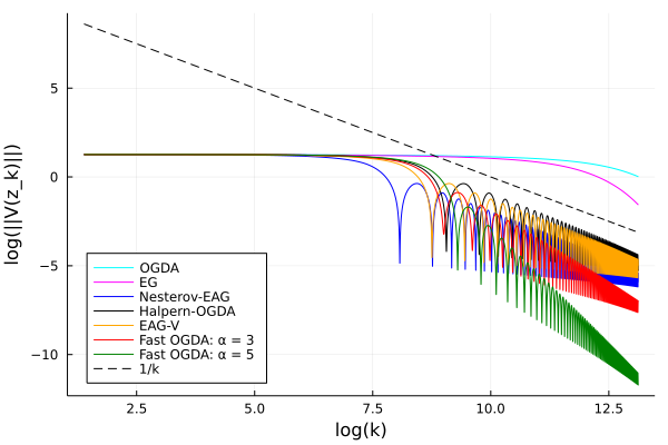
Figure 1: Explicit Fast OGDA outperforms all other explicit methods

For the first numerical experiments we consider the same setting as in [41], namely, we take $n=200$, which means that the underlying space is ${\mathbb{R}}^{400}$, and allow a maximum number of iterations of $5\times 10^{5}$. Figure 1 presents the convergence behaviour of the different methods when solving (111) in logarithmic scale. One can see that the anchoring based methods perform better than the classical algorithms EG and OGDA, and that Nesterov-EAG performs better than Halpern-OGDA, which reconfirms a finding of [39] and is not surprising when one takes into account that the first allows for larger step sizes than EAG-V (and Halpnern-OGDA). On the other hand, Fast OGDA outperforms all the other methods in spite of the fact that the step size is restricted to $\left(0,\frac{1}{2L}\right)$.

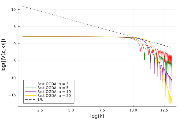
Figure 2: The parameter $\alpha$ influences the convergence behaviour of explicit Fast OGDA

Figure 2 shows that the parameter $\alpha>2$ influences significantly the convergence behaviour of the explicit Fast OGDA algorithm. For this numerical experiment we take $n=1000$, which means that the underlying space is ${\mathbb{R}}^{2000}$, and allow a maximum number of iterations of $5\times 10^{5}$. The speed of convergence increases with increasing $\alpha$ and seem to be much better than $o\left(1/k\right)$. Let us mention that the minimax problem (111) was constructed to show lower complexity bounds of first order methods for convex-concave saddle point problems.

For Nesterov’s dynamical systems with $\frac{\alpha}{t}$ as damping coefficient and the corresponding numerical algorithms approaching the minimization of a smooth and convex function, it is known that $\alpha$ influences in the same way the convergence rates of the objective function values. Another intriguing similarity with Nesterov’s continuous and discrete schemes is the evident oscillatory behaviour of the trajectories, however, there for the objective function values, while for explicit Fast OGDA for the norm of the operator along the trajectory/sequence of generated iterates. This suggests that Nesterov’s acceleration approach can improve the convergence behaviour of continuous and discrete time approaches beyond the optimization setting.

Appendix A Auxiliary results

We collect in this section some auxiliary results which are used in the analysis of the continuous time and the discrete time models.

The following result can be found in [1, Lemma 5.1].

Lemma 17.

Let $\delta>0$. Suppose that $f\colon\left[\delta,+\infty\right)\to\mathbb{R}$ is locally absolutely continuous, bounded from below, and there exists $g\in\mathbb{L}^{1}\left(\left[\delta,+\infty\right)\right)$ such that for almost every $t\geq\delta$

$$\dfrac{d}{dt}f\left(t\right)\leq g\left(t\right).$$

Then the limit $\lim\limits_{t\to+\infty}f\left(t\right)\in\mathbb{R}$ exists.

Opial’s Lemma ([31]) in continuous form is used in the proof of the weak convergence of the trajectory of the dynamical system (11).

Lemma 18.

Let $\mathcal{S}$ be a nonempty subset of $\mathcal{H}$ and $z\colon\left[t_{0},+\infty\right)\to\mathcal{H}$. Assume that

1. for every $z_{*}\in\mathcal{S}$, $\lim\limits_{t\to+\infty}\left\lVert z\left(t\right)-z_{*}\right\rVert$ exists;

2. every weak sequential cluster point of the trajectory $z\left(t\right)$ as $t\to+\infty$ belongs to $\mathcal{S}$.

Then $z(t)$ converges weakly to a point in $\mathcal{S}$ as $t\to+\infty$.

For the convergence proof of the iterates generated by the two numerical algorithms we use the discrete counterpart of Opial’s Lemma.

Lemma 19.

Let $\mathcal{S}$ be a nonempty subset of $\mathcal{H}$ and $\left(z_{k}\right)_{k\geq 1}$ be a sequence in $\mathcal{H}$. Assume that

1. for every $z_{*}\in\mathcal{S}$, $\lim\limits_{k\to+\infty}\left\lVert z_{k}-z_{*}\right\rVert$ exists;

2. every weak sequential cluster point of the sequence $\left(z_{k}\right)_{k\geq 1}$ as $k\to+\infty$ belongs to $\mathcal{S}$.

Then $\left(z_{k}\right)_{k\geq 1}$ converges weakly to a point in $\mathcal{S}$ as $k\to+\infty$.

The following result can be found in [11, Lemma A.2].

Lemma 20.

Let $a>0$ and $q\colon\left[t_{0},+\infty\right)\rightarrow\mathcal{H}$ be a continuously differentiable function such that

$$\lim\limits_{t\to+\infty}\left(q\left(t\right)+\dfrac{t}{a}\dot{q}\left(t\right)\right)=l\in\mathcal{H}.$$

Then it holds $\lim\limits_{t\to+\infty}q\left(t\right)=l$.

The discrete counterpart of this result is stated below. We provide a proof for it, as we could not find any reference for this result in the literature.

Lemma 21.

Let $a\geq 1$ and $\left(q_{k}\right)_{k\geq 0}$ be a bounded sequence in $\mathcal{H}$ such that

$$\lim\limits_{k\to+\infty}\left(q_{k+1}+\dfrac{k}{a}\left(q_{k+1}-q_{k}\right)\right)=l\in\mathcal{H}.$$

Then it holds $\lim\limits_{k\to+\infty}q_{k}=l$.

Proof.

For every $k\geq 0$ we set $r_{k}:=q_{k}-l$. We fix $\varepsilon>0$. Then there exists $k_{0}\geq 1$ such that for every $k\geq k_{0}$

$$\left\lVert r_{k+1}+\dfrac{k}{a}\left(r_{k+1}-r_{k}\right)\right\rVert\leq\varepsilon.$$

Multiplying both side by $ak^{a-1}$, we obtain for every $k\geq k_{0}$

$$\left\lVert\left(ak^{a-1}+k^{a}\right)r_{k+1}-k^{a}r_{k}\right\rVert\leq\varepsilon ak^{a-1}.$$

Then by applying the triangle inequality and using the fact that $\overline{r}:=\sup_{k\geq 0}\left\lVert r_{k}\right\rVert<+\infty$, we deduce that for every $k\geq k_{0}$

$$\left\lVert\left(k+1\right)^{a}r_{k+1}-k^{a}r_{k}\right\rVert\leq\varepsilon ak^{a-1}+\left\lvert\left(k+1\right)^{a}-k^{a}-ak^{a-1}\right\rvert\overline{r}.$$ (112)

The Lagrange error bound of a Taylor series says that for every $k\geq k_{0}$ there exists $m_{k}\in\left(k,k+1\right)$ such that

$$\left\lvert\left(k+1\right)^{a}-k^{a}-ak^{a-1}\right\rvert\leq\dfrac{1}{2}a\left\lvert a-1\right\rvert m_{k}^{a-2}.$$

From here we consider two cases.

Then for every $k\geq k_{0}$ and every $m\in\left(k,k+1\right)$ we have $m^{a-2}\leq 1$ and thus (112) leads to

$$\left\lVert\left(k+1\right)^{a}r_{k+1}-k^{a}r_{k}\right\rVert\leq\varepsilon ak^{a-1}+\dfrac{1}{2}a\left\lvert a-1\right\rvert\overline{r}.$$

We choose $K\geq k_{0}$ and use a telescoping sum argument to get

$$\left\lVert\left(K+1\right)^{a}r_{K+1}-k_{0}^{a}r_{k_{0}}\right\rVert =\left\lVert\displaystyle\sum\limits_{k=k_{0}}^{K}\Bigl{(}\left(k+1\right)^{a}r_{k+1}-k^{a}r_{k}\Bigr{)}\right\rVert\leq\displaystyle\sum\limits_{k=k_{0}}^{K}\left\lVert\left(k+1\right)^{a}r_{k+1}-k^{a}r_{k}\right\rVert$$

$$\leq\varepsilon a\displaystyle\sum\limits_{k=k_{0}}^{K}k^{a-1}+\dfrac{1}{2}a\left\lvert a-1\right\rvert\overline{r}\displaystyle\sum\limits_{k=k_{0}}^{K}1\leq\varepsilon a\left(K+1\right)^{a}+\dfrac{1}{2}a\left\lvert a-1\right\rvert\overline{r}\left(K+1\right).$$

Once again, using the triangle inequality, we conclude that

$$\left\lVert r_{K+1}\right\rVert \leq\dfrac{1}{\left(K+1\right)^{a}}\left\lVert\left(K+1\right)^{a}r_{K+1}-k_{0}^{a}r_{k_{0}}\right\rVert+\dfrac{k_{0}^{a}}{\left(K+1\right)^{a}}\left\lVert r_{k_{0}}\right\rVert\leq\varepsilon a+\dfrac{a\left\lvert a-1\right\rvert\overline{r}}{2\left(K+1\right)^{a-1}}+\dfrac{k_{0}^{a}\overline{r}}{\left(K+1\right)^{a}}.$$

For for every $k\geq k_{0}$ and every $m\in\left(k,k+1\right)$ we have $m^{a-2}\leq\left(k+1\right)^{a-2}$, hence (112) leads to

$$\left\lVert\left(k+1\right)^{a}r_{k+1}-k^{a}r_{k}\right\rVert\leq\varepsilon ak^{a-1}+\dfrac{1}{2}a\left(a-1\right)\overline{r}\left(k+1\right)^{a-2}.$$

We choose also in this case $K\geq k_{0}$ and by a similar argument as above we have that

$$\left\lVert\left(K+1\right)^{a}r_{K+1}-k_{0}^{a}r_{k_{0}}\right\rVert =\left\lVert\displaystyle\sum\limits_{k=k_{0}}^{K}\Bigl{(}\left(k+1\right)^{a}r_{k+1}-k^{a}r_{k}\Bigr{)}\right\rVert\leq\displaystyle\sum\limits_{k=k_{0}}^{K}\left\lVert\left(k+1\right)^{a}r_{k+1}-k^{a}r_{k}\right\rVert$$

$$\leq\varepsilon a\displaystyle\sum\limits_{k=k_{0}}^{K}k^{a-1}+\dfrac{1}{2}a\left(a-1\right)\overline{r}\displaystyle\sum\limits_{k=k_{0}}^{K}\left(k+1\right)^{a-2}$$

$$\leq\varepsilon a\left(K+1\right)^{a-1}\displaystyle\sum\limits_{k=0}^{K}1+\dfrac{1}{2}a\left(a-1\right)\overline{r}\left(K+1\right)^{a-2}\displaystyle\sum\limits_{k=0}^{K}1$$

$$\leq\varepsilon a\left(K+1\right)^{a}+\dfrac{1}{2}a\left(a-1\right)\overline{r}\left(K+1\right)^{a-1}.$$

This leads to

$$\left\lVert r_{K+1}\right\rVert\leq\varepsilon a+\dfrac{a\left(a-1\right)\overline{r}}{2\left(K+1\right)}+\dfrac{k_{0}^{a}\overline{r}}{\left(K+1\right)^{a}}.$$

Therefore, in both scenarios we obtain

$$\limsup_{k\to+\infty}\left\lVert r_{k}\right\rVert\leq\varepsilon a,$$

which leads to the desired conclusion, as $\varepsilon>0$ was arbitrarily chosen. ∎

The following result is a particular instance of [12, Lemma 5.31].

Lemma 22.

Let $\left(a_{k}\right)_{k\geq 1}$, $\left(b_{k}\right)_{k\geq 1}$ and $\left(d_{k}\right)_{k\geq 1}$ be sequences of real numbers. Assume that $\left(a_{k}\right)_{k\geq 1}$ is bounded from below, and $\left(b_{k}\right)_{k\geq 1}$ and $\left(d_{k}\right)_{k\geq 1}$ are nonnegative sequences such that $\sum_{k\geq 1}d_{k}<+\infty$. If

$$a_{k+1}\leq a_{k}-b_{k}+d_{k}\quad\forall k\geq 1,$$

then the following statements are true:

1. the sequence $\left(b_{k}\right)_{k\geq 1}$ is summable, namely $\sum_{k\geq 1}b_{k}<+\infty$;

2. the sequence $\left(a_{k}\right)_{k\geq 1}$ is convergent.

The following elementary result is used several times in the paper.

Lemma 23.

Let $a,b,c\in\mathbb{R}$ be such that $a\neq 0$ and $b^{2}-ac\leq 0$. The following statements are true:

1. if $a>0$, then it holds

   $$a\left\lVert x\right\rVert^{2}+2b\left\langle x,y\right\rangle+c\left\lVert y\right\rVert^{2}\geq 0\quad\forall x,y\in\mathcal{H};$$

2. if $a<0$, then it holds

   $$a\left\lVert x\right\rVert^{2}+2b\left\langle x,y\right\rangle+c\left\lVert y\right\rVert^{2}\leq 0\quad\forall x,y\in\mathcal{H}.$$

References

- [1] B. Abbas, H. Attouch, B.F. Svaiter. Newton-like dynamics and forward–backward methods for structured monotone inclusions in Hilbert spaces. Journal of Optimization Theory and Applications 161(2), 331–360 (2014)
- [2] A. S. Antipin. On a method for convex programs using a symmetrical modification of the Lagrange function. Ekonomika i Matematicheskie Metody 12, 1164–1173 (1976)
- [3] H. Attouch, A. Cabot. Convergence of a relaxed inertial forward–backward algorithm for structured monotone inclusions. Applied Mathematics Optimization 80(3), 547–598 (2019)
- [4] H. Attouch, Z. Chbani, J. Fadili, H. Riahi. First-order optimization algorithms via inertial systems with Hessian driven damping. Mathematical Programming, https://doi.org/10.1007/s10107-020-01591-1
- [5] H. Attouch, Z. Chbani, J. Fadili, H. Riahi. Convergence of iterates for first-order optimization algorithms with inertia and Hessian driven damping. Optimization https://doi.org/10.1080/02331934.2021.2009828
- [6] H. Attouch, Z. Chbani, H. Riahi. Fast proximal methods via time scaling of damped inertial dynamics. SIAM Journal on Optimization 29(3), 2227–2256 (2019)
- [7] H. Attouch, S. C. László. Continuous Newton-like inertial dynamics for monotone inclusions. Set-Valued and Variational Analysis 29(3), 555–581 (2021)
- [8] H. Attouch, S. C. László. Newton-like inertial dynamics and proximal algorithms governed by maximally monotone operators. SIAM Journal on Optimization 30(4), 3252–3283 (2021)
- [9] H. Attouch, J. Peypouquet. The rate of convergence of Nesterov’s accelerated forward-backward method is actually faster than . SIAM Journal on Optimization 26(3), 1824–1834 (2016)
- [10] H. Attouch, J. Peypouquet. Convergence of inertial dynamics and proximal algorithms governed by maximally monotone operators. Mathematical Programming 174(1-2), 391–432 (2019)
- [11] H. Attouch, J. Peypouquet, P. Redont. Fast convex optimization via inertial dynamics with Hessian driven damping. Journal of Differential Equations 261(10), 5734–5783 (2016)
- [12] H.H. Bauschke, P.L. Combettes. Convex Analysis and Monotone Operator Theory in Hilbert Spaces. CMS Books in Mathematics, Springer, New York (2017)
- [13] A. Böhm, M. Sedlmayer, E. R. Csetnek, R. I. Boţ. Two steps at a time–taking GAN training in stride with Tseng’s method. arXiv:2006.09033
- [14] T. Chavdarova, M. I. Jordan, M. Zampetakis. Last-Iterate Convergence of Saddle Point Optimizers via High-Resolution Differential Equations. OPT2021: The 13th Annual Workshop on Optimization for Machine Learning (2021)
- [15] N. Golowich, S. Pattathil, C. Daskalakis. Tight last-iterate convergence rates for no-regret learning in multi-player games. arXiv:2010.13724
- [16] N. Golowich, S. Pattathil, C. Daskalakis, A. Ozdaglar. Last iterate is slower than averaged iterate in smooth convex-concave saddle point problems. In Conference on Learning Theory, PMLR, 1758–1784 (2020)
- [17] I. J. Goodfellow, J. Pouget-Abadie, M. Mirza, B. Xu, D. Warde-Farley, S. Ozair, A. Courville, Y. Bengio. Generative Adversarial Networks. NIPS 2014: Advances in Neural Information Processing Systems 27, 2672–2680 (2014)
- [18] E. Gorbunov. N. Loizou, G. Gidel. Extragradient method: last-iterate convergence for monotone variational inequalities and connections with cocoercivity. AISTATS 2022: The 25th International Conference on Artificial Intelligence and Statistics (2022)
- [19] O. Güler. On the convergence of the proximal point algorithm for convex minimization. SIAM Journal on Control and Optimization 29(2), 403–419 (1991)
- [20] O. Güler. New proximal point algorithms for convex minimization. SIAM Journal on Optimization 2(4), 649–664 (1992)
- [21] B. Halpern. Fixed points of nonexpanding maps. Bulletin of the American Mathematical Society 73(6), 957–961 (1967)
- [22] D. Kim. Accelerated proximal point method for maximally monotone operators. Mathematical Programming 190, 57–87 (2021)
- [23] G. M. Korpelevich. An extragradient method for finding saddle points and for other problems. Ekonomika i Matematicheskie Metody 12(4), 747–756 (1976)
- [24] S. Lee, D. Kim. Fast extra gradient methods for smooth structured nonconvex-nonconcave minimax problems. NIPS 2021: Advances in Neural Information Processing Systems 34 (2021)
- [25] A Madry, A Makelov, L Schmidt, D Tsipras, A Vladu. Towards Deep Learning Models Resistant to Adversarial Attacks. ICLR 2018: International Conference on Learning Representations (2018)
- [26] Y. Malitsky, M. K. Tam. A forward-backward splitting method for monotone inclusions without cocoercivity. SIAM Journal on Optimization 30(2), 1451–1472 (2020)
- [27] Y. Nesterov. A method of solving a convex programming problem with convergence rate . Soviet Mathematics Doklady 27, 372–376 (1983)
- [28] Y. Nesterov. Introductory Lectures on Convex Optimization. Springer, New York (2004)
- [29] Y. Nesterov. Dual extrapolation and its applications to solving variational inequalities and related problems. Mathematical Programming 109, 319–344 (2007)
- [30] S. Omidshafiei, J. Pazis, C. Amato, J. P. How, J. Vian. Deep Decentralized Multi-task Multi-Agent Reinforcement Learning under Partial Observability. Proceedings of the 34th International Conference on Machine Learning, PMLR 70, 2681–2690 (2017).
- [31] Z. Opial. Weak convergence of the sequence of successive approximations for nonexpansive mappings. Bulletin of the American Mathematical Society 73, 591–597 (1967)
- [32] Y. Ouyang , Y. Xu. Lower complexity bounds of first-order methods for convex-concave bilinear saddle-point problems. Mathematical Programming 185, 1–35 (2021)
- [33] J. Park, E. K. Ryu. Exact Optimal Accelerated Complexity for Fixed-Point Iterations. arXiv:2201.11413
- [34] L. D. Popov. A modification of the Arrow–Hurwicz method for search of saddle points. Mathematical Notes of the Academy of Sciences of the USSR 28(5), 845–848 (1980)
- [35] R. T. Rockafellar Monotone operators associated with saddle-functions and minimax problems. In Nonlinear Functional Analysis, Part 1, F. E. Browder (ed.). Proceedings of Symposia in Pure Mathematics 18, American Mathematical Society, 241–250 (1970)
- [36] G. R. Sell, Y. You. Dynamics of Evolutionary Equations. Springer, New York (2002)
- [37] B. Shi, S. Du, M. I. Jordan, W.J. Su Understanding the acceleration phenomenon via high-resolution differential equations. Mathematical Programming https://doi.org/10.1007/s10107-021-01681-8
- [38] W. Su, S. Boyd, E. Candès A differential equation for modeling Nesterov’s accelerated gradient method: theory and insights. Journal of Machine Learning Research 17(153), 1–43 (2016)
- [39] Q. Tran-Dinh. The connection between Nesterov’s accelerated methods and Halpern fixed-point iterations. arXiv:2203.04869
- [40] Q. Tran-Dinh, Y. Luo. Halpern-type accelerated and splitting algorithms for monotone inclusions. arXiv:2110.08150
- [41] T. H. Yoon, E. K. Ryu. Accelerated algorithms for smooth convex-concave minimax problems with rate on squared gradient norm. International Conference on Machine Learning, 12098–12109 (2021)