Antiferromagnetic helix as an efficient spin polarizer: Interplay between electric field and higher ordered hopping

Abstract

We report spin filtration operation considering an antiferromagnetic helix system, possessing zero net magnetization. Common wisdom suggests that for such a system, a spin-polarized current is no longer available from a beam of unpolarized electrons. But, once we apply an electric field perpendicular to the helix axis, a large separation between up and down spin energy channels takes place which yields a high degree of spin polarization. Such a prescription has not been reported so far to the best of our concern. Employing a tight-binding framework to illustrate the antiferromagnetic helix, we compute spin filtration efficiency by determining spin selective currents using Landauer-Büttiker formalism. Geometrical conformation plays an important role in spin channel separation, and here we critically investigate the effects of short-range and long-range hoppings of electrons in presence of the electric field. We find that the filtration performance gets improved with increasing the range of hopping of electrons. Moreover, the phase of spin polarization can be altered selectively by changing the strength and direction of the electric field, and also by regulating the physical parameters that describe the  antiferromagnetic helix. Finally, we explore the specific role of dephasing, to make the system more realistic and to make the present communication a self-contained one. Our analysis may provide a new route of getting conformation-dependent spin polarization  possessing longer range hopping of electrons, and can be generalized further to different kinds of other fascinating antiferromagnetic  systems.

I Introduction

After the discovery of the giant magnetoresistance (GMR) effect gmr1 ; gmr2 ; prinz , spintronics becomes a new field of  research in the discipline of condensed matter physics where the spin degree of freedom of an electron is explored along with its  charge wolf ; spin1 ; spin2 ; spin3 . In conventional electronic devices, Joule heating is an inevitable effect due to the flow of electrons which causes a sufficient power loss. But, if we utilize electron spin instead of the charge, then power will be consumed and at the same time operation will be much faster spin1 ; spin2 . Two pivotal features for the consideration of spin-based electronic devices rather than conventional charged-based ones are: (i) saving more power and information can be transferred at a much faster rate which  undoubtedly reduces cost price by a significant amount and (ii) size of the devices becomes too small so that a large number of  functional elements can be integrated into a small dimension wolf ; spin1 . For instance, the hard disk drive made in 1957 was  able to store data only up to $3.75$ megabytes, and it occupied a volume of $68$ cubic feet. Whereas, a recent hard disk drive  possessing a volume of the order of $2.1$ cubic inches can even store data up to several terabytes hd . Using the GMR phenomenon, not only in storing devices but significant development has been made in different other technologies involving electron spin spin1 ; spin2 ; spin3 .

One of the most fundamental issues in spintronics is to find an efficient route for the separation of two spins, or more precisely we can say, the generation of polarized spin current from a completely unpolarized electron beam. Several propositions have already been made along this line curr1 ; curr2 ; fm1 . The most common practice is to use ferromagnetic materials, though there are several unavoidable limitations fm2 . For instance, a large resistivity mismatch occurs across a junction formed by ferromagnetic and non-magnetic materials, which hinders the proper injection of electrons into the system fm2 ; fm3 . The other crucial limitation arises when we think about the tuning spin selective junction currents. Usually, this is done by means of an external magnetic field, but for a quantum regime, it is very hard to confine a strong magnetic field, and the problem still persists even today. Over the last few years, the use of ferromagnetic materials significantly gets suppressed when spin-orbit (SO) coupled systems came into the picture. Two different kinds of SO interactions are taken into account in solid-state materials, one is known as Rashba rashba and the other one is referred to as Dresselhaus SO interaction dres ; soi . The latter type appears due to the breaking of bulk inversion symmetry of a system, whereas the previous one arises due to the breaking of the symmetry in confining potential. Among these two, the Rashba strength can be tuned externally by suitable setups gate1 ; gate2 , and therefore, the Rashba SO coupled systems draw significant attention than the Dresselhaus ones in the field of spintronics. Different kinds of systems starting from tailor-made geometries, organic and  inorganic molecules have been considered as functional elements in two-terminal as well as multi-terminal setups, and many interesting features have been explored multi1 ; multi2 ; multi3 . But, in most of these cases, especially in molecular systems, the major concern is that the SO coupling strength is too weak compared to the electronic hopping strength, almost an order of magnitude smaller strength . Moreover, the variation of the SO coupling strength is also quite limited by external means. Because of these facts, a high degree of spin polarization and its possible tuning in a wide range are quite difficult to achieve in SO coupled systems, though there are of course many other advantages that make these systems promising functional elements in spintronics.

To avoid all these issues, modern machinery has concentrated on antiferromagnetic (AF) materials that possess an alternate type of magnetic ordering and have zero net magnetization afm1 ; afm2 ; afm3 . Several key prospects of using an AF system as a spin-polarized functional element are there. For instance, these materials are insensitive to external magnetic fields, and they are much faster and can be operated up to a high-frequency range ($\sim$THz) than the traditional ferromagnetic systems thz . Moreover, due to the absence of any stray fields, a large number of closely packed functional elements can be accommodated in a small region which leads to several important advantages in designing efficient electronic devices based on spin-based transport phenomena. Nowadays, antiferromagnetic spintronics evolves as a cutting-edge research field, and, may lead to new prospects in the magnetic community afm4 ; afm5 ; afm6 ; afm7 .

In the present work, we propose a new prescription for efficient spin filtration considering an antiferromagnetic system, which we refer to as an “antiferromagnetic helix” (AFH). The role of chirality on spin filtration first came into realization based on the experimental work of Göhler et al. dna where they have shown that almost $60\%$ spin polarization can be achieved through a self-assembled monolayers of double-stranded DNA molecules deposited on a gold substrate. They have described this effect as chiral induced spin selectivity (CISS). After this realization, several experimental and theoretical research groups have paid significant attention to this CISS effect, considering different kinds of molecular as well as artificially designed systems, possessing helical  geometry prl ; protein ; bacteria ; dna1 ; helix ; aprotein ; edge ; sarkar ; magfield . But, to the best of our knowledge, no effort has been made so far to address the phenomenon of spin filtration considering a ‘magnetic helix structure with vanishing net magnetization’, and this is precisely the fundamental motivation behind the present work. For our AFH, simulated by a tight-binding framework, magnetic moments in alternate lattice sites are arranged in opposite directions, resulting in a zero net magnetization. In such a system, common wisdom suggests that spin filtration is no longer possible. But, interestingly we find that, once we apply an electric field perpendicular to the helix axis, a large separation between two spin channels takes place, which results in a high degree of spin polarization. The central mechanism relies on the helicity and the applied electric field. In the absence of any of these two, helicity and electric field, no such phenomenon is observed.

Determining spin-dependent transmission probabilities using the well-known Green’s function formalism gf1 ; gff1 ; gf2 , we compute spin selective currents through the AFH following the Landauer-Büttiker prescription gf3 ; gf4 . From the currents, we evaluate the spin  polarization coefficient. The geometrical conformation plays a significant role in spin filtration, and we investigate it by considering both short- and long-range hopping cases. From our analysis, we find that the spin filtration efficiency gets enhanced with increasing electron hopping among more lattice sites. The specific roles of all other physical quantities are thoroughly discussed which lead to several interesting features. Finally, to make the quantum system more realistic and for the sake of completeness of our study, we include the effects of electron dephasing dephase1 ; dephase2 ; dephase3 ; dephase4 ; dephase5 on spin polarization. Our analysis may provide some key inputs towards designing efficient spintronic devices considering different kinds of antiferromagnetic helical systems, possessing longer range hopping of electrons.

The rest part of the work is arranged as follows.

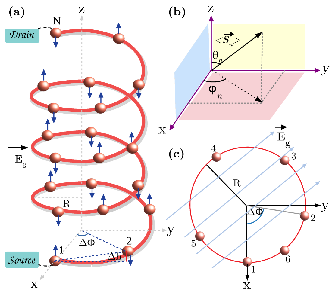
Figure 1: (Color online). (a) A right-handed antiferromagnetic helix is clamped between two one-dimensional non-magnetic electrodes, namely, source and drain. $R$ being the radius of the helix, and $\Delta\phi$ and $\Delta h$ correspond to the twisting angle and stacking distance between the magnetic sites (colored balls), respectively. Successive magnetic moments, shown by the blue arrows, associated with the magnetic sites are arranged along $+Z$ and $-Z$ directions, resulting in a vanishing net magnetization. An electric field of strength $E_{g}$ is applied perpendicular to the helix axis, which plays a pivotal role in spin filtration. (b) Orientation of the net spin $\langle\boldsymbol{\vec{S}_{n}}\rangle$ in spherical polar coordinate system. (c) Projection of the right-handed helix on the $X$-$Y$ plane.

Section II includes the spin-polarized setup, tight-binding (TB) Hamiltonian of the junction, and the required theoretical prescriptions for the calculations. All the results are presented and thoroughly discussed in Sec. III. Finally, the essential findings are summarized in Sec. IV.

II Quantum system, TB Hamiltonian and theoretical formulation

II.1 Junction setup and the TB Hamiltonian

Let us begin with the spin-polarized setup shown in Fig. 1(a), where an antiferromagnetic (AF) system is coupled to the source and drain electrodes. The magnetic sites (filled colored balls) in the AF system are arranged in a helical pattern. Each of these sites contains a finite magnetic moment, denoted by the blue arrow, associated with a net spin $\langle\vec{\boldsymbol{S}_{n}}\rangle$. The successive magnetic moments are aligned in opposite directions ($\pm Z$), and therefore, the net magnetization of the helix becomes zero. We refer to this system as an “antiferromagnetic helix” (AFH), and here in our work, we will show how such an AFH acts for spin filtration. The general orientation of any local spin $\langle\vec{\boldsymbol{S}_{n}}\rangle$, and hence the magnetic moment, can be illustrated by the usual co-ordinate system as presented in Fig. 1(b), where $\theta_{n}$ and $\varphi_{n}$ are the polar and azimuthal angles, respectively.

Two essential physical parameters characterize the helical geometry prl ; protein those are $\Delta\phi$ and $\Delta h$ (see Fig. 1), where the first one represents the twisting angle and the other parameter denotes the stacking distance. Depending on $\Delta h$, we can have a helical system where lower or higher-order hopping of electrons becomes significant. When $\Delta h$ is very small i.e., atoms in the helix are densely packed, electrons can hop at multiple sites, which is referred to as ‘long-range hopping antiferromagnetic helix’ (LRH AFH). On the other hand, when the atoms are less densely packed viz, $\Delta h$ is quite large, electrons can hop between a few neighboring magnetic sites. Such a system is called a ‘short-range hopping antiferromagnetic helix’ (SRH AFH). In the present work, we consider these two different kinds of AF helices and investigate the results.

The antiferromagnetic helix is subjected to an electric field, having strength $E_{g}$, perpendicular to the helix axis. It plays a central role in spin filtration, and it can be understood from our forthcoming discussion. With a suitable setup, one can tune  the strength of this field as well as its direction.

In order to investigate spin dependent transport phenomena and to exhibit the spin filtration operation, the helical system is clamped between source and drain electrodes. We describe this nanojuntion using the tight-binding framework sk1 ; sk2 ; sk3 ; skm1 . The TB Hamiltonian of the full system is written as a sum

$$\boldsymbol{\mathit{H}}=\boldsymbol{\mathit{H}}_{AFH}+\boldsymbol{\mathit{H}}_{S}+\boldsymbol{\mathit{H}}_{D}+\boldsymbol{\mathit{H}}_{tun}$$ (1)

where different sub-Hamiltonians in the right side of Eq. 1 are associated with different parts of the nanojunction and they are described as follows.

The term $\boldsymbol{\mathit{H}}_{AFH}$ corresponds to the Hamiltonian of the antiferromagnetic helix. For an AFH, be it a short-range or a long-range one, the TB Hamiltonian is expressed as

$$\boldsymbol{\mathit{H}}_{AFH}=\sum_{n}\boldsymbol{c}_{n}^{\dagger}\left(\boldsymbol{\epsilon}_{n}-\boldsymbol{\vec{\mathpzc{h}}}_{n}\cdot\boldsymbol{\vec{\sigma}}\right)\boldsymbol{c}_{n}$$

$$+\sum_{n=1}^{N-1}\sum_{m=1}^{N-n}\left(\boldsymbol{c}_{n}^{\dagger}\boldsymbol{t}_{m}\boldsymbol{c}_{n+m}+h.c.\right).$$ (2)

where $\boldsymbol{c}_{n}^{\dagger}=\left(c_{n\uparrow}^{\dagger}\quad c_{n\downarrow}^{\dagger}\right)$. $c_{n\sigma}^{\dagger}$ $(c_{n\sigma})$ is the creation (annihilation) operator of an electron at site $n$ with spin $\sigma\left(=\uparrow,\downarrow\right)$. $\boldsymbol{\epsilon}_{n}-\vec{\boldsymbol{\mathpzc{h}}}_{n}\cdot\vec{\boldsymbol{\sigma}}$ is the effective site energy matrix which looks like

$$\boldsymbol{\epsilon}_{n}-\vec{\boldsymbol{\mathpzc{h}}}_{n}\cdot\vec{\boldsymbol{\sigma}}=\begin{pmatrix}\epsilon_{n}-\mathpzc{h}\cos\theta_{n}&-\mathpzc{h}\sin\theta_{n}e^{-i\varphi_{n}}\\ -\mathpzc{h}\sin\theta_{n}e^{i\varphi_{n}}&\epsilon_{n}+\mathpzc{h}\cos\theta_{n}\end{pmatrix}$$ (3)

where $\epsilon_{n}$ is the on-site energy in the absence of any kind of magnetic scattering. $\boldsymbol{\vec{\mathpzc h}}_{n}=J\langle\boldsymbol{\vec{S}}_{n}\rangle$, called as the spin-flip scattering parameter where $J$ is the coupling strength strength between the coupling of an itinerant electron with local magnetic moment, associated with the average spin $\langle\boldsymbol{\vec{S}}_{n}\rangle$. $\vec{\boldsymbol{\sigma}}$ is the Pauli spin vector. Here we assume that $\boldsymbol{\sigma}_{z}$ is diagonal. The term $\vec{\boldsymbol{\mathpzc{h}}}_{n}\cdot\vec{\boldsymbol{\sigma}}$ represents the  spin-dependent scattering and it is widely used in literature sk1 ; sk2 ; sk3 ; skm1 . The key point is that the strength ‘$J$’ is reasonably large than the other spin-dependent scattering parameters viz, SO coupling, Zeeman splitting in presence of magnetic field, etc strength . Thus, there is a possibility of getting a high degree of spin filtration under suitable input condition(s), in the presence of a spin-moment scattering mechanism.

The second term of Eq. 2, involving $\boldsymbol{t}_{m}$, is quite tricky, not like usual nearest-neighbor hopping case, and the summations over $n$ and $m$ need to take carefully. $\boldsymbol{t}_{m}$ is a $(2\times 2)$ hopping matrix, and it becomes

$$\boldsymbol{t}_{m}=\begin{pmatrix}t_{m}&0\\ 0&t_{m}\end{pmatrix}$$ (4)

where $t_{m}$ represents the hopping between the sites $n$ and $(n+m)$. The hopping strength $t_{m}$ is written as prl ; protein

$$t_{m}=t_{1}\textrm{e}^{-(l_{m}-l_{1})/l_{c}}$$ (5)

where $t_{1}$ is the nearest-neighbor hopping integral, $l_{m}$ is the distance of separation between the sites $n$ and $(n+m)$, $l_{1}$ is the distance among the nearest-neighbor sites and $l_{c}$ is the decay constant. In terms of the radius $R$ (see Fig. 1(c) where the projection of the helix in the $X$-$Y$ plane is shown), twisting angle $\Delta\phi$ and the stacking distance $\Delta h$, $l_{m}$ gets the form prl ; protein ; edge

$$l_{m}=\sqrt{{[2R\sin(m\Delta\phi/2)}]^{2}+(m\Delta h)^{2}}.$$ (6)

When the AFH is subjected to a transverse electric field, its site energies get modified. The effective site energy for any site $n$ becomes aprotein ; edge

$$\epsilon_{n}^{\rm eff}=\epsilon_{n}+eV_{g}\cos(n\Delta\phi-\beta)$$ (7)

where $e$ is the electronic charge, and, $V_{g}$ ($=2E_{g}R$) is the gate voltage, responsible for the generation of the electric field. $\beta$ represents the angle between the incident electric field and the positive $X$-axis prl ; protein .

The TB Hamiltonians of the side attached source (S) and drain (D) electrodes, $\boldsymbol{\mathit{H}}_{S}$ and $\boldsymbol{\mathit{H}}_{D}$ and their coupling with the AFH ($\boldsymbol{\mathit{H}}_{tun}$) look quite simple than what is described above for the antiferromagnetic helix. The electrodes are assumed to be perfect, one-dimensional, and non-magnetic in nature. They are expressed as,

$$\boldsymbol{\mathit{H}}_{S}=\boldsymbol{\mathit{H}}_{D}=\sum_{n}\boldsymbol{a}_{n}^{\dagger}\boldsymbol{\epsilon}_{0}\boldsymbol{a}_{n}+\sum_{n}\left(\boldsymbol{a}_{n+1}^{\dagger}\boldsymbol{t}_{0}\boldsymbol{a}_{n}+h.c.\right)$$ (8)

where $\boldsymbol{\epsilon}_{0}={\rm diag}(\epsilon_{0},\epsilon_{0})$ and $\boldsymbol{t}_{0}={\rm diag}(t_{0},t_{0})$. $\epsilon_{0}$ and $t_{0}$ are the on-site energy and nearest-neighbor hopping integral, respectively. $\boldsymbol{a}_{n}^{\dagger}=\left(a_{n\uparrow}^{\dagger}\quad a_{n\downarrow}^{\dagger}\right)$, $a_{n\sigma}$’s are the usual fermionic operators in the electrodes.

Finally, the tunneling Hamiltonian is expressed as

$$\boldsymbol{\mathit{H}}_{tun}=t_{S}\left(\boldsymbol{c}_{1}^{\dagger}\boldsymbol{a}_{-1}+h.c.\right)+t_{D}\left(\boldsymbol{c}_{N}^{\dagger}\boldsymbol{a}_{N+1}+h.c.\right)$$ (9)

where $t_{S}$ and $t_{D}$ are the coupling strengths of the AFH with S and D, respectively. We refer to the lattice site of the source which is coupled to the helix as $-1$ and the site of the drain which is attached to the helix as $N+1$. The sites $1,2\dots N$ ($N$ being the total number of magnetic sites) are used for the AFH.

II.2 Theoretical formulation

In order to inspect spin-dependent transport phenomena and spin polarization coefficient, the first and foremost thing that we need to calculate is the two-terminal transmission probability. We compute it using the well known non-equilibrium Green’s function formalism gf1 ; gff1 ; gf2 ; gf3 ; gf4 . In terms of retarded and advanced Green’s functions, $\boldsymbol{\mathit{G}}^{r}$ and $\boldsymbol{\mathit{G}}^{a}$, the spin-dependent transmission coefficient is obtained from the expression gf1 ; gff1 ; gf4

$$T_{\sigma\sigma^{\prime}}=\textrm{Tr}\left[\boldsymbol{\Gamma}_{S}\boldsymbol{\mathit{G}}^{r}\boldsymbol{\Gamma}_{D}\boldsymbol{\mathit{G}}^{a}\right]$$ (10)

where,

$$\boldsymbol{\mathit{G}}^{r}=\left(\boldsymbol{\mathit{G}}^{a}\right)^{\dagger}=\left[\boldsymbol{E}-\boldsymbol{\mathit{H}}_{AFH}-\boldsymbol{\Sigma}_{S}-\boldsymbol{\Sigma}_{D}\right]^{-1}.$$ (11)

$\boldsymbol{\Sigma}_{S}$ and $\boldsymbol{\Sigma}_{D}$ are the self-energy matrices gf1 ; gff1 ; gf2 which capture all the essential information of the electrodes and their coupling with the helix. $\boldsymbol{\Gamma}_{S}$ and $\boldsymbol{\Gamma}_{D}$ are the coupling matrices.

For an incoming electron with spin $\uparrow$, two things may occur. We can have a finite possibility of getting up spin electron as a up spin or it can be flipped. Similar options are also available for an injected down spin electron. Thus, considering pure $(T_{\sigma\sigma})$ and spin flip $(T_{\sigma\sigma^{\prime}})$ transmissions, we can write the net up and down spin transmission probabilities ($T_{\uparrow}$ and $T_{\downarrow}$) as

$$T_{\uparrow} =T_{\uparrow,\uparrow}+T_{\downarrow,\uparrow}$$ (12a)

$$T_{\downarrow} =T_{\downarrow,\downarrow}+T_{\uparrow,\downarrow}.$$ (12b)

From the transmission coefficients $T_{\uparrow}$ and $T_{\downarrow}$, we evaluate up and down spin junction currents, using the Landauer Büttiker prescription gf1 ; gff1 ; gf2 ; gf3 ; gf4 . The spin-dependent current, when a finite bias $V$ is applied across the AFH, is expressed as

$$I_{\sigma}=\frac{e}{h}\int T_{\sigma}\left(f_{S}-f_{D}\right)dE$$ (13)

where, $f_{S}$ and $f_{D}$ are the Fermi functions, associated with S and D, respectively, and they are

$$f_{S(D)}=\frac{1}{1+\textrm{e}^{\left(E-\mu_{S(D)}\right)/k_{B}\mathsf{T}}}.$$ (14)

Here $\mu_{S}$ and $\mu_{D}$ are the electro-chemical potentials of S and D, respectively, and $k_{B}\mathsf{T}$ is the thermal energy.

Determining $I_{\uparrow}$ and $I_{\downarrow}$, we evaluate spin filtration efficiency following the relation dephase3

$$P=\frac{I_{\uparrow}-I_{\downarrow}}{I_{\uparrow}+I_{\uparrow}}\times 100\%.$$ (15)

When only up spin electrons propagate we get $P=100\%$, while for the situation where only down spin electrons get transferred through the AFH, we get $P=-100\%$. For the situation where both up and down spin electrons propagate equally, no spin filtration occurs. We want to reach the limiting value where $P=100\%$ or $-100\%$, which is usually very hard to achieve.

Inclusion of dephasing: Dephasing is an important factor and in many cases, it cannot be avoided especially when we think about the experimental realization of a theoretical proposal. There are different possible routes through which a system is disturbed by dephasing, and it is thus required to incorporate its effect in our analysis. Several methodologies dephase1 ; dephase2 ; dephase3 ; dephase4 ; dephase5 are available for the inclusion of dephasing and most of them are very complex. Büttiker on the other hand predicted phenomenologically a very simple but elegant way to incorporate the dephasing effect into the system dephase1 ; dephase2 , and here we use the same procedure. In this prescription it is assumed that each lattice site of the AFH is attached to a dephasing electrode, commonly referred to as Büttiker probe. The key concept is that the dephasing electrodes will not drag or inject any finite number of electrons into the system i.e., the net current passing through such electrodes becomes exactly zero dephase1 ; dephase2 . Electrons from the AFH enter into the dephasing electrodes, and after losing their phase memories, they eventually come back to the parent system.

In order to achieve the zero current condition in different dephasing electrodes, we need to choose the voltages $V_{n}$ ($V_{n}$ being the voltage at $n$th dephasing electrode) in the appropriate way aprotein ; gff1 . The $V_{n}$’s are determined following the Landauer-Büttiker current expression gf1 ; gff1 associated with each dephasing electrode, and evaluating the bias drop at different lattice sites of the helix. It is crucial to point out that, the evaluation of this bias drop is quite complicated as it is a non-linear problem. The prescription can be simplified to some extent by considering a linear profile along the helix, which is most commonly used in literature, and here in our present work we also follow it. Suppose a finite voltage $V_{0}$ is applied between the real electrodes $S$ and $D$, and (say) $V_{S}=V_{0}$ and $V_{D}=0$, without loss of any generality. Then, the voltages $V_{n}$ at different lattice sites can be calculated without much difficulty, as we assume the linear drop, and adjusting these voltages across the dephasing electrodes, the zero-current condition is established (a more detailed discussion about it is available in aprotein ; gff1 ).

In presence of the Bütiker probes, the transmission probability of getting electrons at the drain electrode (D) is modified aprotein ; dephase5 , and it becomes

$$T_{\sigma\sigma^{\prime}}^{eff}(V)=\sum_{\alpha=S,n}T_{\sigma\sigma^{\prime}}^{\alpha D}(V)\frac{V_{\alpha}}{V_{0}}.$$ (16)

The transmission probabilities are now voltage dependent, and thus, special care has to be taken to calculate these quantities vt1 ; vt2 . Here $T_{\sigma\sigma^{\prime}}^{SD}(V)$ and $T_{\sigma\sigma^{\prime}}^{nD}(V)$ denote the transmission probabilities from the source electrode (S) and from the $n$-th dephasing electrode to the drain end, respectively. The dephasing electrodes are connected at all the lattice sites of the antiferromagnetic helix, apart from the sites $1$ and $N$ where the real electrodes (S, D) are attached. In our formulation, the coupling strength between the AFH and the dephasing electrode is mentioned by the parameter $\eta$, and it describes the dephasing strength.

To compute $T_{\sigma\sigma^{\prime}}^{eff}(V)$, an important step must be performed which is as follows. For a biased system, since the scattering states become the eigenstates of the biased Hamiltonian, the site energy $\epsilon_{0}$ needs to be shifted by $V_{0}$ in the source electrode, and by $V_{n}$ in the $n$-th Büttiker probe vt1 ; vt2 . Using Eq. 16, we get the effective up and down spin transmission probabilities, at different voltages, from the relations

$$T_{\uparrow}^{eff}(V) =T_{\uparrow,\uparrow}^{eff}(V)+T_{\downarrow,\uparrow}^{eff}(V)$$ (17a)

$$T_{\downarrow}^{eff}(V) =T_{\downarrow,\downarrow}^{eff}(V)+T_{\uparrow,\downarrow}^{eff}(V).$$ (17b)

The effective spin-dependent current in presence of dephasing can thus be obtained through the expression

$$I_{\sigma}(V)=\frac{e}{h}\int T_{\sigma}^{eff}(V)\left(f_{S}-f_{D}\right)dE.$$ (18)

With the effective spin-dependent currents, the same definition is followed as mentioned in Eq. 15, to compute spin polarization coefficient $P$ in the presence of dephasing.

In the extreme low biased condition, the above current equation (Eq. 18) for any $q$-th electrode, be it real or virtual, boils down to aprotein

$$I_{\sigma}^{q}(V)=\frac{e^{2}}{h}\sum_{\alpha}T_{\sigma}^{\alpha q}(V_{\alpha}-V_{q})$$ (19)

where the voltages $V_{\alpha}$ and $V_{q}$ can be derived from the prescription given above. In this limiting condition, the current is ‘linearly’ proportional to the voltage. On the other hand, in the limit of high bias, Eq. 18 cannot be simplified in the linear form like what is given in Eq. 19, and we get the non-linear behavior. For the sake of completeness of our analysis, we discuss the accuracy of the above prescription in the appropriate sub-section.

III Numerical Results and Discussion

Now we present our results and investigate the specific role of the external electric field on spin filtration, under different input conditions. Both the short-range and long-range antiferromagnetic helices are taken into account. For these two types of AFHs, we choose the geometrical parameters $R$, $\Delta h$, and $\Delta\phi$ as given in Table 1. These parameter values are analogous to  the real helical systems like single-stranded DNA and protein molecules, and they are the most suitable examples where respectively the  short-range and long-range hopping models are taken into account prl ; protein . A large amount of investigation has already been done in the literature considering this particular set of parameter values in different contemporary works, and accordingly, here also we select these typical values. Other sets of parameter values represent the  SRH and LRH of electrons can also be considered, and all the physical pictures studied here will remain unaltered.

The other physical parameters those are common throughout the analysis are as follows. In the absence of electric field, the on-site

Table 1: Geometrical parameters describing the SRH and LRH AFHs.

System	$R$ (nm)	$\Delta h$ (nm)	$\Delta\phi$ (rad)	$l_{c}$ (nm)
SRH AFH	$0.7$	$0.34$	$\pi/5$	$0.09$
LRH AFH	$0.25$	$0.10$	$5\pi/9$	$0.09$

energies ($\epsilon_{n}$) in the AFH are set to zero, and we fix the NNH strength $t_{1}=1\,$eV. The spin dependent scattering parameters $\mathpzc{h}$ is set at $1\,$eV. As already mentioned, the successive magnetic moments in the helix system are aligned in opposite directions ($\pm Z$) (see the schematic diagram given in Fig. 1(a)). We set $\theta_{n}=0$ for all odd $n$ sites, and $\theta_{n}=\pi$ for all the even $n$ sites. The azimuthal angle $\varphi_{n}$ is fixed to zero for all $n$. In the side attached electrodes, we choose $\epsilon_{0}=0$, $t_{0}=2\,$eV. The coupling parameters $t_{S}$ and $t_{D}$ are set at $1\,$eV. All the other energies are also measured in units of electron-volt (eV). Unless specified, the results are worked out considering a right-handed antiferromagnetic helix with $\beta=0$ and in the absence of dephasing. We set the system temperature at $100\,$K, throughout the discussion.

III.1 Spin dependent transmission probabilities and spin polarization coefficient

Let us begin with spin-dependent transmission probabilities, shown in the first column of Fig. 2, where Fig. 2(a) and Fig. 2(c) are associated with the SRH and LRH AFHs respectively. The corresponding spin polarization coefficients are presented in the right column. All these results are evaluated for the electric field-free condition i.e. when $V_{g}=0$. For both the helix systems we find that up and down spin transmission probabilities, shown by the black and cyan colors respectively, exactly overlap with each other, resulting in a vanishing spin polarization. This is expected, as for such helices the symmetry between the up and down spin sub-Hamiltonians ($\boldsymbol{H}_{\uparrow}$ and $\boldsymbol{H}_{\downarrow}$) is preserved. Accordingly, we get an identical set of energy eigenvalues  for the two different spin electrons, and thus the transmission probabilities, as the transmission peaks are directly related to the energy eigenvalues of the bridging system. The appearance of identical energy eigenvalues can easily be checked by writing the Hamiltonian of the AFH  ($\boldsymbol{\mathit{H}}_{AFH}$) as a sum of the two sub-Hamiltonians (viz, $\boldsymbol{\mathit{H}}_{AFH}=\boldsymbol{\mathit{H}}_{\uparrow}+\boldsymbol{\mathit{H}}_{\downarrow}$), one is associated with up spin electrons and the other is involved with the down spin ones. In the absence of the electric field, these two sub-Hamiltonians are effectively identical to each other, and hence, the same set of energy channels is obtained. For a particular AFH, the sharpness of different transmission peaks depends on the coupling ($t_{S}$ and $t_{D}$) of the helix to the side attached electrodes. With increasing the coupling, the transmission peaks get more broadened, and the broadening due to this coupling is always higher than

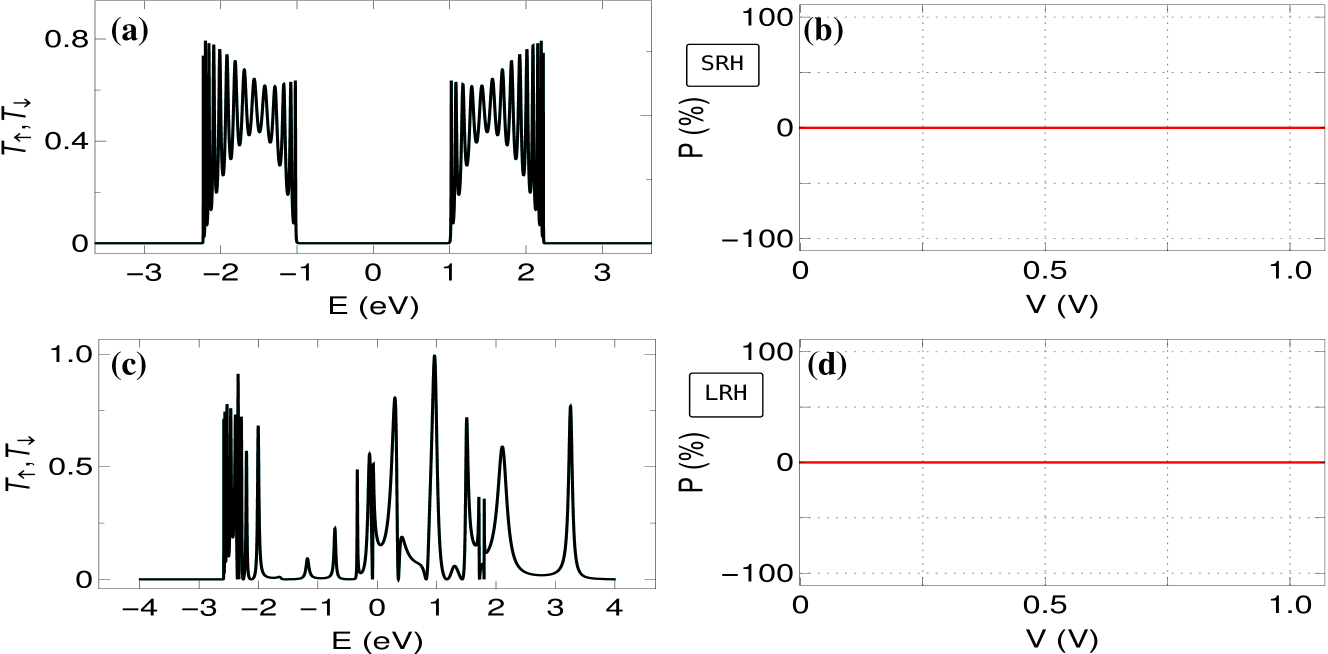
Figure 2: (Color online). Zero field case: Spin dependent transmission probabilities as a function of energy for (a) SRH and (c) LRH AFHs, where the black and cyan colors are associated with the up and down spin electrons, respectively. The up and down spin transmission spectra get exactly overlapped with each other for each AFH. The corresponding spin polarization coefficients with bias voltage are shown in (b) and (d), respectively. Spin polarization drops to zero for the entire voltage window. Here we choose $E_{F}=-0.9\,$eV and set $N=30$. The dephasing strength $\eta=0$.

that caused by the thermal effect. In our numerical calculation since $t_{S}$ and $t_{D}$ are comparable to $t_{1}$ (strong coupling limit), any significant change with increasing temperature is not expected and therefore we restrict our calculation at a moderate temperature.

Depending on the specific range of electron hopping, we get a contrasting nature in the transmission peaks and their arrangements over the energy window. For the chosen set of parameter values, electrons can able to hop in a few neighboring lattice sites in the SRH system, and for this case, the transmission peaks are quite uniformly spaced and peaked as well. More regular behavior is obtained as we move towards the NNH model. A finite and large gap is obtained across $E=0$, following the energy gap in the SRH system. This is quite analogous to the binary alloy system where alternate sites possess two different energies and repeat it throughout the system, due to the antiferromagnetic ordering. But, once the higher-order hopping of electrons is taken into account, like what is considered for the LRH system, the sharp gap around $E=0$ disappears. At the same time, the uniformity is lost significantly. Along one edge of the energy window, the transmission peaks are closely packed whereas large gaps between the peaks are obtained along the other edge of the window protein . All these characteristics are the generic features of a long-range hopping system. This asymmetric distribution, on the other hand, plays an important role to achieve a favorable response in spin polarization, which can be visualized in the forthcoming discussion.

The situation drastically changes, once we apply an electric field. In Fig. 3 we show the results, for the same set of systems as taken in Fig. 2, considering the gate voltage $V_{g}=0.6$ V. Several notable features are obtained those are illustrated one by one as follows. At a first glance, we find that up and down spin transmission probabilities get separated both for the SRH and LRH helices, as clearly reflected from the spectra given in Figs. 3(a) and (c), where two different colors are associated with two

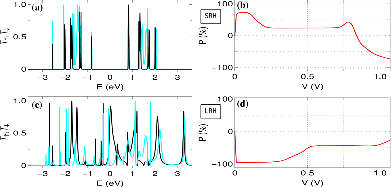
Figure 3: (Color online). Results in the presence of electric field with $V_{g}=0.6\,$V. In (a) and (c), spin selective transmission probabilities as a function of energy are shown for (a) SRH and (c) LRH AFHs, where the black and cyan colors are associated with up and down spin electrons, respectively. The corresponding $P$-$V$ curves are shown in (b) and (d), respectively. All the other physical parameters are the same as taken in Fig. 2.

different spin electrons. In the presence of electric field, site energies get modified in a cosine form, following Eq. 7, which makes the system a disordered (correlated) one aah1 ; aah2 ; aah3 . Due to this disorder, the symmetry between up and down spin sub-Hamiltonians gets broken, which provides different sets of spin-specific energy channels. Under this situation, a mismatch occurs  between the spin-dependent transmission spectra. Apparently, it seems that the separation between the up and down spin transmission  peaks is not that much large, what we generally expect from ferromagnetic systems, but selectively placing the Fermi energy, we can  have the possibility of getting a reasonably high degree of spin filtration. This is precisely shown in Figs. 3(b) and (d). Both for  the SRH and LRH AFHs, large spin polarization is obtained over a particular voltage range, but the response becomes more favorable  for the case of LRH AFH. This is entirely due to the non-uniform distribution of the transmission peaks around the center of the spectrum.  So, naturally, starting from an NNH AFH, we can expect a better response whenever we include an additional hopping of electrons, and  we confirm it through our detailed numerical calculations. Moreover, it is pertinent to note that, the cosine modulation in site energies due to the electric field makes the system a non-trivial one, as it generates a fragmented energy spectrum (which is the generic feature of the well-known Aubry-André-Harper (AAH) model aah1 ; aah2 ; aah3 ). This behavior helps us to find a high degree of spin polarization even at multiple Fermi energies.

The key conclusion that is drawn from the above analysis is that the breaking of the symmetry between up and down spin sub-Hamiltonians in the AFH entirely depends on the external electric field which makes the system a disordered (correlated) one. In the absence of helicity, the site energies become uniform. Under this situation, the symmetry between the sub-Hamiltonians associated with up and down spin electrons gets preserved, and hence, no such spin filtration phenomenon is obtained.

III.2 Possible tuning of spin polarization

This sub-section deals with the possible tuning of spin filtration efficiency, by adjusting different parameter values associated with the junction setup.

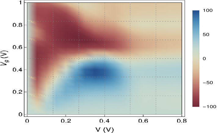
Figure 4: (Color online). Simultaneous variations of $P$ with bias voltage $V$ and gate voltage $V_{g}$ for a $50$-site LRH AFH when $E_{F}$ is fixed at $1\,$eV. The dephasing parameter $\eta=0$.

From the above analysis since it is already established that LRH AFH is superior to the SRH AFH, in the rest part of our discussion we concentrate only on the LRH AFH systems unless stated otherwise.

Figure 4 shows simultaneous variations of spin polarization coefficient $P$ with the bias voltage $V$ and the gate voltage $V_{g}$. Both these two factors play a significant role in spin filtration efficiency. When $V_{g}$ is absolutely zero (i.e., in the absence of electric field) there is no spin polarization as up and down spin sub-Hamiltonians are symmetric. With increasing $V_{g}$, we are expecting a favorable spin polarization, but attention has to be given to the localizing behavior of energy eigenstates. The inclusion of an electric field transforms the AFH from a completely perfect to a correlated disordered system, and thus, for large $V_{g}$ the eigenstates will be almost localized. In that limit, we cannot get spin filtration operation. Hence, we need to restrict $V_{g}$ in such a way that the energy channels are conducting in behavior (see Ref. sarkar for a  comprehensive analysis of electronic localization in SRH and LRH helices in presence of transverse electric field). For a fixed $V_{g}$, when a finite voltage drop is introduced across the junction, we get a non-zero spin polarization depending on the dominating energy channels among up and down spin electrons. With the increase of the bias window, more and more number of both up and down spin channels are available that contribute to the current, and hence, the possibility of mutual cancellations becomes higher which can reduce the degree of spin polarization. Thus, both $V_{g}$ and the bias voltage need to be considered selectively, to have a favorable response.

Like bias voltage $V$, the choice of $E_{F}$ is also very crucial. Our aim is to find a suitable $E_{F}$ where any of the two spin channels dominates over the other, as maximum as it is possible. This, on the other hand, is directly linked with the gate voltage $V_{g}$ as it

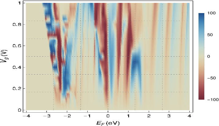
Figure 5: (Color online). Dependence of $P$ with $E_{F}$ and $V_{g}$ when the bias voltage is fixed at $0.2\,$V. The other parameters are: $N=50$ and $\eta=0$.

influences the site energies of the AFH. To have an idea about the selection of $V_{g}$ and $E_{F}$, in Fig. 5 we show the dependence of $P$ on these quantities. The results are computed, setting the voltage drop $V=0.2\,$V. This typical bias voltage is considered due to the fact that here we can get a favorable response as reflected from Fig. 4. We vary $E_{F}$ almost over the entire allowed energy window, and it is seen that for a wide range of $E_{F}$ ($\sim-2\leq E_{F}\leq\sim 2$), a reasonably large $P$ is obtained. Thus, fine tuning of $E_{F}$ is no longer required, which is of course quite important in the context of experimental realization of our proposed setup.

In the same footing it is indeed required to check the filtration efficiency when we simultaneously vary $E_{F}$ and the bias voltage $V$, keeping the gate voltage constant. The results are shown in Fig. 6, where we fix $V_{g}=0.8\,$V. This typical value of $V_{g}$ is chosen observing the favorable response from Figs. 4 and 5. Here also we find that a high degree of spin polarization is achieved at different bias drops across the junction for several distinct choices of Fermi energy $E_{F}$. All these favorable responses are associated with the modifications of the up and down spin energy channels.

Along with the favorable spin polarization, a complete phase reversal (change of sign) of $P$ is also obtained from all these figures (Figs. 4-6) which is due to the swapping of dominating spin channels with the change of the physical parameters.

Now we concentrate on the effect of field direction, which is changed by the parameter $\beta$. The dependence of spin polarization with $\beta$ is presented in Fig. 7, by varying $\beta$ from $0$ to $2\pi$. Almost a regular oscillation is shown providing high peaks ($P\sim 100\%$) and dips ($P\sim-100\%$). The magnitude and sign reversal of $P$ are due to the modifications of spin specific energy

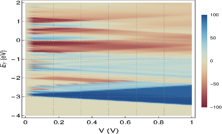
Figure 6: (Color online). Dependence of $P$ with $E_{F}$ and $V$ when the gate voltage is fixed at $0.8\,$V. The other parameters are: $N=50$ and $\eta=0$.

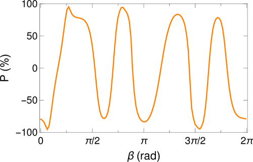
Figure 7: (Color online). Variation of spin polarization ($P$) with the field direction ($\beta$). The other physical parameters are: $E_{F}=0.5\,$eV, $V=0.2\,$V, $V_{g}=0.8\,$V, $N=50$ and $\eta=0$.

channels of the helix with $\beta$ as it is directly related to the site energy (see Eq. 7). It suggests that the spin filtration efficiency can be monitored selectively by changing the field direction, keeping all the other factors unchanged.

Following the above analysis it is found that the helicity and electric field are strongly correlated with each other, and in the absence of any of these two, spin filtration is no longer possible. At this stage, it is indeed required to check the effect of helicity on a more deeper level. In Fig. 8 we show the conformational effect of the helical geometry on spin polarization. We vary $\Delta h$ and $\Delta\phi$ in a reasonable range around the chosen values of these parameters for the LRH AFH, as mentioned in Table 1. The radius $R$ is kept constant which is $0.25\,$nm. The twisting angle $\Delta\phi$ has an important role as it modulates the site energy as well as the hopping integrals. But the more pronounced effect is observed by changing the stacking distance $\Delta h$. With the enhancement of

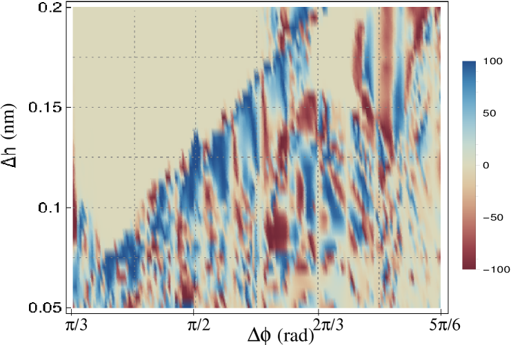
Figure 8: (Color online). Simultaneous variations of $P$ with $\Delta\phi$ and $\Delta h$. Here we choose $E_{F}=0.5\,$eV, $V=0.2\,$V, $V_{g}=0.8\,$V, $N=50$, $\beta=0$ and $\eta=0$.

$\Delta h$, for a fixed $\Delta\phi$, the hopping of electrons in larger sites gradually decreases, and the system approaches the NNH model, providing reduced spin polarization. In the limiting region when electrons can hop only between the nearest-neighbor sites, the spin polarization becomes vanishingly small. Carefully inspecting the density plot given in Fig. 8, it is inferred that the best performance is obtained for low $\Delta h$ when the twisting angle is confined within the range $\sim\pi/2\leq\phi\leq\sim 2\pi/3$. Thus, the helicity and higher-order hopping of electrons are the key aspects to having a high degree of spin filtration.

III.3 Effect of dephasing

To have a more realistic situation, especially considering the experimental facts, in this sub-section we explore the specific role of dephasing dephase1 ; dephase2 ; dephase3 ; dephase4 ; dephase5 that may enter into the system in many ways on spin polarization. Different kinds of interactions of the physical system with external factors can phenomenologically be incorporated through the dephasing effect.

$\blacksquare$ Accuracy checking of theoretical prescription in presence of dephasing: Before presenting the results in the presence of dephasing, it is indeed required to check the accuracy of the theoretical formulation illustrated above in Sec. II. To do that, we consider a spin-less LRH helix with $15$ lattice sites, as a typical example, and compute the currents in all the Büttiker probes (such probes are connected in all the sites of the helix from the site number $2$ to $14$), along with the drain current (red curve). The results are shown in Fig. 9 for the two distinct dephasing strengths that are  presented in (a) and (b), setting the Fermi energy $E_{F}=0.3\,$eV. It is clearly seen that the drain current is reasonably large than  the currents in all the Büttiker probes, and most interestingly we find that the currents in the Büttiker probes are almost zero,

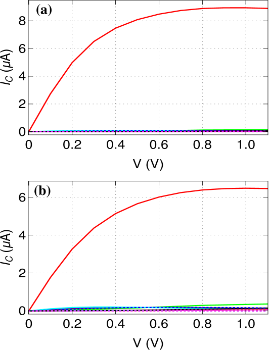
Figure 9: (Color online). Current in the drain electrode (red curve) along with the currents in all the Büttiker probes (other colored curves, not clearly seen as they almost overlap to each other) as a function of bias voltage for a spin-less LRH helix, where (a) $\eta=0.25$ and (b) $\eta=0.5$. The other physical parameters are: $N=15$, $E_{F}=0.3\,$eV and $V_{g}=0$.

even for too high voltages. This is exactly what we are expecting i.e., the vanishing current condition in each dephasing electrode. Thus, we can argue that the theoretical prescription given here can safely be used to study the effect of dephasing.

Now come to the results of AFH in presence of dephasing. Like Fig. 6, in Fig. 10 we show the simultaneous variations of $P$ on the bias voltage $V$ and the Fermi energy $E_{F}$, fixing the dephasing strength $\eta=0.1$. All the other physical parameters are kept unchanged as taken in Fig. 6. The effect of dephasing is quite appreciable. What we see is that the Fermi energy and the bias windows for which a high degree of spin polarization is available in the absence of dephasing (see Fig. 6), get reduced when the dephasing effect is taken into account. The reduction of spin polarization in presence of $\eta$ can be explained as follows. In the Büttiker probe prescription, the effect of dephasing is incorporated by connecting each and every lattice site of the AFH with virtual electrodes. Due to the coupling of the AFH to these virtual electrodes, transmission peaks get broadened, and thus more overlap takes place between the up and down spin channels. Therefore, these two spin-dependent channels contribute to the current, and hence, the spin polarization decreases. A similar kind of dephasing effect (viz, reduction of $P$ with $\eta$) is also obtained when we observe simultaneous variations of $P$ with $V_{g}$ and $V$ keeping $E_{F}$ constant, and, $V_{g}$ and $E_{F}$ considering a fixed bias voltage. Accordingly, here we do not present the density plots of $P$, like what are shown in Fig. 4 and Fig. 5, in the presence of $\eta$ as the role $\eta$ can be guessed in these cases.

Here it is relevant to check the dependence of spin current ($I_{S}=I_{\uparrow}-I_{\downarrow}$) and spin polarization for other values of the dephasing strength $\eta$ as well. The results are given in Figs. 11 (a) and (b), respectively, by varying $\eta$ in a

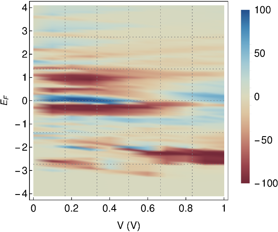
Figure 10: (Color online). A similar kind of density plot, as given in Fig. 6, in the presence of dephasing, with the dephasing strength $\eta=0.1$.

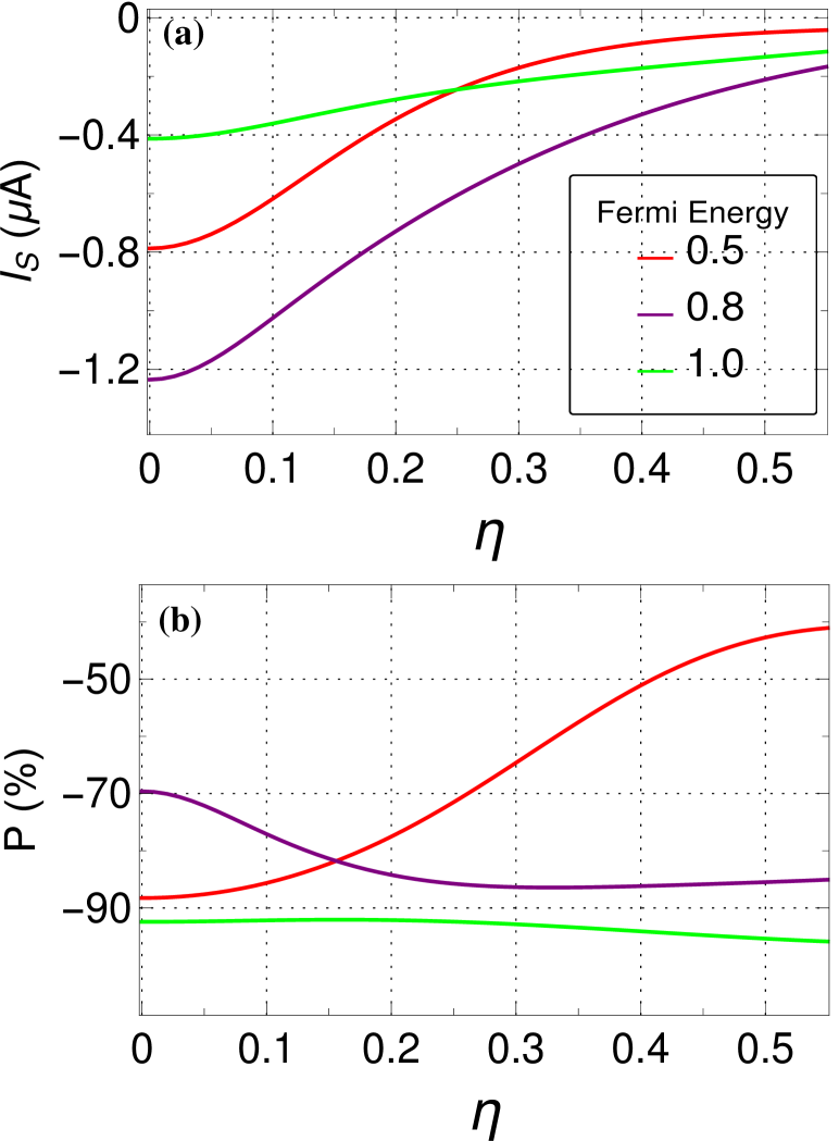
Figure 11: (Color online). (a) Spin current and (b) spin polarization coefficient as a function of dephasing strength $\eta$, at three typical Fermi energies. Here we set $N=50$, $V=0.2\,$V and $V_{g}=0.8\,$V.

reasonable range. Three different Fermi energies are taken into account, those are represented by three different colored curves. It is clearly observed that the spin current decreases with increasing $\eta$, following the above argument of the broadening of both up and down spin transmission peaks and their overlap (Fig. 11(a)). This reduction of spin current can also be implemented by means of phase randomization of the electrons in the virtual electrodes, as originally put forward by Büttiker dephase1 ; dephase2 ; dephase5 . Electrons enter into these electrodes and they come back to the helix system after randomizing their phases, and thus more mixing of the two opposite spin electrons occurs, resulting in a reduced spin current. In the same analogy, the degree of spin polarization gets decreased with increasing the dephasing strength (Fig. 11(b)). From $P$-$\eta$ characteristics it is found that though the spin filtration efficiency gets reduced with $\eta$, still a sufficiently large value of $P$ is obtained even when $\eta$ is reasonably large. Thus, we can safely claim that our proposed quantum system can be utilized as an efficient functional element for spin filtration operation under strong environmental interactions as well as the limit of high temperatures.

III.4 Possible experimental routes of designing AFH

Finally, we refer to some experimental works where different kinds of anti-ferromagnetic systems have been used, aiming to establish confidence that our proposed magnetic helix system can also be realized experimentally. In presence of an external magnetic field, Johnston has reported afhelix1 magnetic properties  and other related phenomena considering an AFH system. There are several experimental works performed by Sangeetha and co-workers,  where they have found helical antiferromagnet in different compounds. For instance in Ref. afhelix2 , Sangeetha et al. have  established a transition from antiferromagnetic to paramagnetic phase using the compound ${\rm EuCo}_{2-y}{\rm As}_{2}$ with spin  $S=7/2$ which possesses a helical shape afhelix2 . In this work, they have measured different physical quantities like magnetic  susceptibility, heat capacities, etc. A high nuclear magneto resistance (NMR) has also been found in that sample nmr . In another  work, Sangeetha and co-workers have established helical antiferromagnetic ordering considering ${\rm EuNi}_{1.95}{\rm As}_{2}$ single  crystal afhelix3 . Goetsch et al. have reported the same in polycrystalline sample ${\rm Lu}_{1-x}{\rm Sc}_{x}{\rm MnSi}$ at  higher Neél’s temperature afhelix4 . The antiferromagnetic helical pattern has also been noticed in an organic molecule.  Lin et al. have reported the canted antiferromagnetic behavior in ${\rm[M(mtpo)_{2}(H_{2}O)_{n}]}$, ${\rm M=Co^{2+}}$ or  ${\rm Ni^{+}}$ with a helical topology afhelix5 . Pylypovskyi et al. have suggested an idea about the tailoring of the geometry  of curvilinear antiferromagnet afhelix6 . This prescription allows substantiating a chiral helimagnet in presence of Dzyloshinskii-Moriya interaction. Considering the helical antiferromagnet sample ${\rm SrFeO}_{3-\delta}$, Zhao et al. have discussed a metal-insulator transition afhelix7 . There exist several other antiferromagnetic helices as well.

Considering all such examples of antiferromagnetic helical systems, we believe that our proposed spin-polarized AFH system can be designed with modern technology and with a suitable laboratory setup.

Here it is relevant to note that all the above-mentioned experimental references contain heavy magnetic elements, and thus one may think whether the tight-binding Hamiltonian mentioned in Eq. 2 can be used to describe our helix systems or not. But the theoretical work studied by Takahashi and Igarashi taka gives us confidence that Eq. 2 can safely be considered, as in that work they have also taken a similar kind of tight-binding Hamiltonian to describe ${\rm La_{2}CuO_{4}}$ and ${\rm Sr_{2}CuO_{2}Cl_{2}}$. There exist several other references as well pic ; cao where tight-binding Hamiltonians have been taken into account for such types of heavy magnetic elements.

IV Summary and outlook

For the first time, we report spin filtration operation considering an antiferromagnetic helical system in presence of an external electric field. Both the short-range and long-range hopping cases are taken into account, associated with the geometrical conformation. Simulating the spin-polarized nanojunction (source-AFH-drain) within a tight-binding framework, we compute spin-dependent transmission probabilities following the well-known Green’s function formalism and the spin-dependent junction currents through the Landauer-Büttiker prescription. From the currents, we evaluate the spin polarization coefficient. To make the proposed quantum system more realistic, we also include the effects of dephasing, and to get the confidence, the accuracy of the theoretical prescription in presence of dephasing is critically checked. Finally, we discuss the possible routes of realizing such an antiferromagnetic helical geometry in a laboratory. Different aspects of spin-dependent transmission probabilities and spin polarization coefficient under different input conditions are critically investigated. The essential findings are listed as follows.
$\bullet$ In the absence of the external electric field, up and down spin sub-Hamiltonians become symmetric and thus no spin  polarization is obtained. Once the symmetry is broken by applying the electric field, finite spin polarization is found.
$\bullet$ Comparing the results between the SRH and LRH AFHs, it is noticed that LRH AFH is much superior to the other. This is essentially due to the irregular distribution of the resonant peaks in the transmission-energy spectrum. The irregularity gradually decreases with lowering the electron hopping among the lattice sites.
$\bullet$ The degree of spin polarization and its phase can be tuned selectively by means of the input parameters, and the notable thing is that a high degree of spin polarization persists over a reasonable range of physical parameters. It clearly suggests that fine tuning of the parameter values is no longer required, and hence we hope that the studied results can be examined in a laboratory.
$\bullet$ The geometrical conformation plays an important role. For the situation when $\Delta\phi$ becomes zero i.e., in the absence of twisting, spin filtration is no longer available.
$\bullet$ Though the degree of spin filtration efficiency gets reduced with increasing the dephasing strength $\eta$, still, reasonably large spin polarization is available, even for moderate $\eta$. It suggests that the proposed functional element can safely be used for spin polarization under strong environmental interactions as well as in the limit of high temperatures.

Our present proposition may help to design efficient spintronic devices using antiferromagnetic helices with longer-range hopping of electrons, and can be generalized to other correlated antiferromagnetic systems as well.

References

- (1) G. Binasch, P. Grünberg, F. Saurenbach, and W. Zinn, Enhanced magnetoresistance in layered magnetic structures with antiferromagnetic interlayer exchange. Phys. Rev. B 39, 4828 (1989).
- (2) A. Fert, Nobel Lecture: Origin, development, and future of spintronics. Rev. Mod. Phys. 80, 1517 (2007).
- (3) G. A. Prinz, Magnetoelectronics. Science 282, 1660 (1998).
- (4) S. A. Wolf, D. D. Awschalom, R. A. Buhrman, J. M. Daughton, S. von Molnár, M. L. Roukes, A. Y. Chtchelkanova, D. M. Treger, Spintronics: a spin-based electronics vision for the future. Science 294, 1488 (2001).
- (5) I. Zutić, J. Fabian, and S. Das Sarma, Spintronics: Fundamentals and applications. Rev. Mod. Phys. 76, 323 (2004).
- (6) Y. Jiao, F. Ma, C. Zhang, J. Bell, S. Sanvito, and A. Du, First-Principles Prediction of Spin-Polarized Multiple Dirac Rings in Manganese Fluoride. Phys. Rev. Lett. 119, 016403 (2017).
- (7) J. Sinova, S. O. Valenzuela, J. Wunderlich, C. H. Back, and T. Jungwirth, Spin Hall effects. Rev. Mod. Phys. 87, 1213 (2015).
- (8) E. Grochowski, and R. D. Halem, Technological impact of magnetic hard disk drives on storage systems. IBM Syst. J. 42, 338 (2003).
- (9) X-F. Ouyang, Z-Y. Song, and Y-Z. Zhang, Fully spin-polarized current in gated bilayer silicene. Phys. Rev. B 98, 075435 (2018).
- (10) S. Kumar, R. L. Kumawat, and B. Pathak, Spin-Polarized Current in Ferromagnetic Half-Metallic Transition- Metal Iodide Nanowires. J. Phys. Chem. C 123, 15717 (2019).
- (11) K. Tsukagoshi, B. Alphenaar, and H. Ago, Coherent transport of electron spin in a ferromagnetically contacted carbon nanotube. Nature 401, 572 (1999).
- (12) S. Kamboj, D. K. Roy, S. Roy, R. R. Chowdhury, P. Mandal, M. Kabir, and G. Sheet, Temperature dependent transport spin-polarization in the low Curie temperature complex itinerant ferromagnet . J. Phys.: Condens. Matter 31, 415601 (2019).
- (13) E. I. Rashba, Theory of electrical spin injection: Tunnel contacts as a solution of the conductivity mismatch problem. Phys. Rev. B 62, R16267 (2000).
- (14) Y. A. Bychkov, and E. I. Rashba, Oscillatory effects and the magnetic susceptibility of carriers in inversion layers. J. Phys. C: Solid State Phys. 17, 6039-6045 (1984).
- (15) G. Dresselhaus, Spin-Orbit Coupling Effects in Zinc Blende Structures. Phys. Rev. 100, 580 (1955).
- (16) A. Machon, H. -C. Koo, J. Nitta, S. M. Frolov, and R. A. Duine, New perspectives for Rashba spin–orbit coupling. Nat. Mater. 14, 871 (2015).
- (17) S. Premasiri, S. K. Radha, S. Sucharitakul, U. R. Kumar, R. Sankar, F. -C. Chou, Y. -T. Chen, and X. P. A. Gao, Tuning Rashba Spin–Orbit Coupling in Gated Multilayer InSe. Nano Lett. 7, 4403 (2018).
- (18) S. Ganguly, and S. K. Maiti, Selective spin transmission through a driven quantum system: A new prescription. J. Appl. Phys. 129, 123902 (2021).
- (19) B. K. Nikolić, L. P. Zârbo, and S. Souma, Imaging mesoscopic spin Hall flow: Spatial distribution of local spin currents and spin densities in and out of multiterminal spin-orbit coupled semiconductor nanostructures. Phys. Rev. B 73, 075303 (2006).
- (20) P. Földi, O. Kálmán, M. G. Benedict, and F. M. Peeters, Quantum rings as electron spin beam splitters. Phys. Rev. B 73, 155325 (2006).
- (21) M. Dey, S. K. Maiti, S. Sil, and S. N. Karmakar, Spin-orbit interaction induced spin selective transmission through a multi-terminal mesoscopic ring. J. Appl. Phys. 114, 164318 (2013).
- (22) Y.-H. Su, S.-H. Chen, C. D. Hu, and C.-R. Chang, Competition between spin–orbit interaction and exchange coupling within a honeycomb lattice ribbon. J. Phys. D: Appl. Phys. 49, 015305 (2015).
- (23) V. Baltz, A. Machon, M. Tsoi, T. Moriyama, T. Ono, and Y. Tserkovnyak, Antiferromagnetic spintronics. Rev. Mod. Phys. 90, 015005 (2018).
- (24) T. Jungwirth, J. Sinova, X. Matri, J. Wunderlich, and C. Felser, The multiple directions of antiferromagnetic spintronics. Nat. Phys. 14, 200 (2018).
- (25) M. B. Jungfleisch, W. Zhang, and A. Hoffmann, Perspectives of antiferromagnetic spintronics. Phys. Lett. A 382, 865 (2018).
- (26) P. Y. Artemchuk, O. R. Sulymenko, S. Louis, J. Li, R. S. Khymyn, E. Bankowski, T. Meitzler, V. S. Tyberkevych, A. N. Slavin, and O. V. Prokopenko, Terahertz frequency spectrum analysis with a nanoscale antiferromagnetic tunnel junction. J. Appl. Phys. 127, 063905 (2020).
- (27) P. Wadley, B. Howells, J. Zelezný, C. Andrews, V. Hills, R. P. Campion, V. Novák, K. Olejník, F. Maccherozzi, S. S. Dhesi, S. Y. Martin, T. Wagner, J. Wunderlich, F. Freimuth, Y. Mokrousov, J. Kunes, J. S. Chauhan, M. J. Grzybowski, A. W. Rushforth, K. W. Edmonds, B. L. Gallagher, and T. Jungwirth, Electrical switching of an antiferromagnet. Science 351, 587 (2016).
- (28) P. Nmec, M. Fiebig, T. Kampfrath, and A. V. Kimel, Antiferromagnetic opto-spintronics. Nat. Phys. 14, 229 (2018).
- (29) T. Kosub, M. Kopte, and R. Hühne, Purely antiferromagnetic magnetoelectric random access memory. Nat Commun 8, 13985 (2017).
- (30) D. D. Gupta, and S. K. Maiti, Can a sample having zero net magnetization produce polarized spin current?. J. Phys.: Condens. Matter 32, 505803 (2020).
- (31) B. Göhler, V. Hamelbeck, T. Z. Markus, M. Kettner, G. F. Hanne, Z. Vager, R. Naaman, and H. Zacharias, Spin Selectivity in Electron Transmission Through Self-Assembled Monolayers of Double-Stranded DNA. Science 331, 894 (2011).
- (32) A. -M. Guo, and Q. -F. Sun, Spin-Selective Transport of Electrons in DNA Double Helix. Phys. Rev. Lett. 108, 218102 (2012).
- (33) A. -M. Guo, and Q. -F. Sun, Spin-dependent electron transport in protein-like single-helical molecules. Proc. Natl. Acad. Sci. 111, 11658 (2014).
- (34) D. Mishra, T. Z. Markus, R. Naaman, M. Kettner, B. Göhler, H. Zacharias, N. Friedman, M. Sheves, and C. Fontanesi, Spin-dependent electron transmission through bacteriorhodopsin embedded in purple membrane. Proc. Natl. Acad. Sci. 110, 14872 (2013).
- (35) E. Medina, F. López, M. A. Ratner, and V. Mujica, Chiral molecular films as electron polarizers and polarization modulators. Europhys. Lett. 99, 17006 (2012).
- (36) R. Gutierrez, E. Díaz, R. Naaman, and G. Cuniberti, Spin-selective transport through helical molecular systems. Phys. Rev. B 85, 081404 (2012).
- (37) T. -R. Pan, A. -M. Guo, and Q. -F. Sun, Effect of gate voltage on spin transport along -helical protein. Phys. Rev. B 92, 115418 (2015).
- (38) A. -M. Guo, and Q. -F. Sun, Topological states and quantized current in helical organic molecules. Phys. Rev. B 95, 155411 (2017).
- (39) S. Sarkar, and S. K. Maiti, Localization to delocalization transition in a double stranded helical geometry: effects of conformation, transverse electric field and dynamics. J. Phys.: Condens. Matter 32, 505301 (2020).
- (40) H. Simchi, M. Esmaeilzadeh, and H. Mazidabadi, The effect of a magnetic field on the spin-selective transport in double-stranded DNA. J. Appl. Phys. 115, 204701 (2014).
- (41) S. Datta, Electronic Transport in Mesoscopic Systems (Cambridge University Press, Cambridge, 1997).
- (42) S. Datta, Quantum Transport: Atom to Transistor (Cambridge University Press, Cambridge, 2005).
- (43) D. S. Fisher, and P. A. Lee, Relation between conductivity and transmission matrix. Phys. Rev. B 23, 6851 (1981).
- (44) M. D. Ventra, Electrical Transport in Nanoscale Systems, Cambridge University Press, Cambridge (2008).
- (45) B. K. Nikolić, and P. B. Allen, Quantum transport in ballistic conductors: evolution from conductance quantization to resonant tunnelling. J. Phys.: Condens. Matter 12, 9629 (2000).
- (46) M. Büttiker, Role of quantum coherence in series resistors. Phys. Rev. B 33, 3020 (1986).
- (47) M. Büttiker, Coherent and sequential tunneling in series barriers. BM J. Res. Dev. 32, 63 (1988).
- (48) D. Rai, and M. Galperin, Spin inelastic currents in molecular ring junctions. Phys. Rev. B 86, 045420 (2012).
- (49) M. Dey, S. K. Maiti, and S. N. Karmakar, Effect of dephasing on electron transport in a molecular wire: Green’s function approach. Org. Electron. 12, 1017 (2011).
- (50) M. Patra, S. K. Maiti, and S. Sil, Engineering magnetoresistance: a new perspective. J. Phys.: Condens. Matter 31, 355303 (2019).
- (51) A. A. Shokri, M. Mardaani, and K. Esfarjani, Spin filtering and spin diode devices in quantum wire systems. Physica E 27, 325 (2005).
- (52) A. A. Shokri, M. Mardaani, Spin-flip effect on electrical transport in magnetic quantum wire systems. Solid State Commun. 137, 53 (2006).
- (53) M. Mardaani, A. A. Shokri, Theoretical approach on spin-dependent conductance in a magnetic-quantum wire. Chem. Phys. 324, 541 (2006).
- (54) M. Sarkar, M. Dey, S. K. Maiti, and S. Sil, Engineering spin polarization in a driven multistranded magnetic quantum network. Phys. Rev. B 102, 195435 (2020).
- (55) P. F. Bagwell and T. P. Orlando, Landauer’s conductance formula and its generalization to finite voltages. Phys. Rev. B 40, 1456 (1989).
- (56) G. B. Lesovik and I. A. Sadovskyy, Scattering matrix approach to the description of quantum electron transport. Phys. Usp. 54, 1007 (2011).
- (57) S. Ganeshan, K. Sun, and S. Das Sarma, Topological Zero-Energy Modes in Gapless Commensurate Aubry-André-Harper Model. Phys. Rev. Lett. 110, 180403 (2013).
- (58) X. Li, and S. Das Sarma, Mobility edges in one-dimensional bichromatic incommensurate potentials. Phys. Rev. B 96, 085119 (2017).
- (59) X. Li, S. Ganeshan, J. H. Pixley and S. Das Sarma. Many-Body Localization and Quantum Nonergodicity in a Model with a Single-Particle Mobility Edge. Phys. Rev. Lett. 115, 186601 (2015).
- (60) D. C. Johnston, Magnetic structure and magnetization of helical antiferromagnets in high magnetic fields perpendicular to the helix axis at zero temperature. Phys. Rev. B 96, 104405 (2017).
- (61) N. S. Sangeetha, V. K. Anand, C. R. Eduardo, V. Smetana,A. -V. Mudring, and D. C Johnston, Enhanced moments of Eu in single crystals of the metallic helical antiferromagnet . Phys. Rev. B 97, 144403 (2018).
- (62) Q. -P. Ding, N. Higa, N. S. Sangeetha, D. C. Johnston, and Y. Furukawa, NMR determination of an incommensurate helical antiferromagnetic structure in . Phys. Rev. B 95, 184404 (2017).
- (63) N. S. Sangeetha, V. Smetana, A. -V. Mudring, and D. C. Johnston, Helical antiferromagnetic ordering in single crystals. Phys. Rev. B 100, 094438 (2019).
- (64) R. J. Goetsch, V. K. Anand, D. C. Johnston, Helical antiferromagnetic ordering in . Phys. Rev. B 90, 064415 (2014).
- (65) Q. -P. Lin, J. Zhang, X. -Y. Cao, Y. -G. Yao, Z. -J. Li, L. Zhang, and Z. -F. Zhou, Canted antiferromagnetic behaviours in isostructural Co( II ) and Ni( II ) frameworks with helical lvt topology. Cryst. Eng. Comm. 12, 2938 (2010).
- (66) O. V. Pylypovskyi, D. Y. Kononenko, K. V. Yershov, U. K. Röbler, A. V. Tomilo, J. Fassbender, J. V. D. Brink, D. Makarov, and D. D. Sheka, Curvilinear one-dimensional antiferromagnets. Nano. Lett. 20, 8157 (2020).
- (67) Y. M. Zhao, and P. F. Zhou, Metal–insulator transition in helical antiferromagnet. J. Magn. Magn. Mater. 281, 214 (2004).
- (68) M. Takahashi and J. Igarashi, Local approach to electronic excitations in the insulating copper oxides and . Phys. Rev. B 59, 7373 (1999).
- (69) M. J. DeWeert, D. A. Papaconstantopoulos, and W. E. Pickett, Tight-binding Hamiltonians for high-temperature superconductors and applications to coherent-potential-approximation calculations of the electronic properties of . Phys. Rev. B 39, 4235 (1989).
- (70) C. Cao, P. J. Hirschfeld, and H. -P. Cheng, Proximity of antiferromagnetism and superconductivity in : Effective Hamiltonian from ab initio studies, Phys. Rev. B 77, 220506(R) (2008).