Statistical classification for Raman spectra of tumoral genomic DNA

Abstract

We exploit Surface–Enhanced Raman Scattering (SERS) to investigate aqueous droplets of genomic DNA deposited onto silver–coated silicon nanowires and we show that it is possible to efficiently discriminate between spectra of tumoral and healthy cells. To assess the robustness of the proposed technique, we develop two different statistical approaches, one based on the Principal Component Analysis of spectral data and one based on the computation of the $\ell^{2}$ distance between spectra. Both methods prove to be highly efficient and we test their accuracy via the so–called Cohen’s $\kappa$ statistics. We show that the synergistic combination of the SERS spectroscopy and the statistical analysis methods leads to efficient and fast cancer diagnostic applications allowing a rapid and unexpansive discrimination between healthy and tumoral genomic DNA alternative to the more complex and expensive DNA sequencing.

Keywords: Tumoral genomic DNA; Raman spectroscopy; classification; Principal Component Analysis; logistic regression; minimum distance classifiers.

1 Introduction

The relevance of Raman spectroscopy in medical diagnostics [1], and in particular in the study of cancer diseases [2], has been widely pointed out in the recent pertinent literature. The potentiality of this technique lies in its label–free character, which allows to directly analyse biological samples and obtain unaltered information about their physico–chemical properties.

Here, we exploited Raman spectroscopy to investigate aqueous droplets of genomic DNA deposited onto silver–coated silicon nanowires (Ag/SiNWs). By following the same experimental procedure proposed in [3], we use Raman mapping to collect several spectra that are statistically analyzed here to discriminate between samples extracted from tumoral and healthy cells.

Raman spectroscopy is an inelastic optical scattering technique, which records the light scattered from vibrations in molecules or optical phonons in solids [4, 5]. These inelastic scattering processes have small cross section and, thus, the typical intensity of Raman signals is very low [6]. On the other hand, as it was firstly shown in [7], due to electromagnetic and chemical effects, the Raman signal coming from molecules adsorbed on a metal nanostructure can be increased by several order of magnitude. This phenomenon, known as Surface–Enhanced Raman Scattering (SERS) [8, 9], has been exploited in our experiment by dripping the DNA aqueous solution on a substrate made of a disordered array of silver–coated silicon nanowires, whose effectiveness in enhancing the Raman signal has been recently demonstrated in a series of experimental studies, e.g., [10, 11, 12, 13, 14, 15, 16].

In this way we are able to collect Raman maps of the deposited drops composed of several good quality Raman spectra which, although very similar among each others, allow us to distinguish between drops of healthy and tumoral DNA. Anyway the major challenge of this approach is that the Raman mapping generates large data sets that need an advanced data processing to extract meaningful information allowing us the discrimination between the healthy and tumor DNA sample.

The aim of this work is thus to build a binary classification model aimed to discriminate, with high accuracy, spectra coming from different DNA molecules, corresponding to the outcomes of a target variable taking values 0 and 1 for healthy and tumoral samples respectively.

Our proposal is based on two different methods. The first one reduces initially the amount of predictors by means of a Principal Components Analysis (PCA). After reducing dimensionality, the new variables are exploited to build a logistic regression model, whose outcome is the desired classifier. The second method involves the full data set to exploit the geometric features of the Raman spectra. Indeed the classifier adopted in this case is based on the computation of the $\ell^{2}$ distance between test samples and the spectral average of healthy and tumoral training spectra. We will show that both the strategies achieve a very high accuracy, close to 90%.

The paper is organized as follows: in Section 2 we discuss experimental and statistical methods, mainly focusing on the latter. Our results are discussed in Section 3, whereas in Section 4 we summarize our conclusions.

2 Methods

In this section we describe the processes and approaches that we have developed in the different steps of our study. We shall provide a very short account of the sample preparation procedure and the Raman measurements, referring to [3] for a thorough and detailed description. On the other hand, we shall discuss in detail the statistical approach developed to analyze the experimental data, which is the true novel contribution provided in this paper.

2.1 Experimental procedures

Plasma enhanced chemical vapor deposition (PECVD) was used to grow Au catalyzed SiNWs on Si wafers, kept at $350^{\textup{o}}$C, using SiH₄ and H₂ as precursors. The coating was realized by evaporating an Ag film onto SiNWs arrays with nominal thickness of $100$ nm.

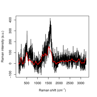
Figure 1: Comparison between a raw Raman spectrum and the curve (in red) obtained by performing Savitzky–Golay filtering.

As skin cancer model [17] we used the human melanoma cell line SK–MEL–28, which was compared to the human immortalized keratinocyte HaCaT as control health skin model. After standard culture, harvesting, and centrifugation, cell pellets were obtained and used to extract the genomic DNA, that, on turn, was re–suspended in DNase free water to obtain a $20$ ng$/\mu$L solution.

The final samples are prepared by depositing one drop of the DNA solution on Ag/SiNWs substrates coming from the very same batch.

Each droplet is spectrally mapped after drying by means of a DXR2xi Thermo Fisher Scientific Raman Imaging Microscope equipped with a $532$ nm excitation laser and a $50\times$ objective. For each droplet, Raman spectra are collected at points on a square grid with spacing $4~{}\mu$m, at $1$ mW laser power and performing four accumulations lasting $5$ ms each.

2.2 Data set and conveyed information

As data set we have considered $N=3980$ spectra, 1990 from the tumoral and 1990 from the healthy DNA droplet. The spectra have been randomly chosen in the central part of the droplets, since in this region the biological layer formed after dehydration happens to be thinner, so that the interaction between the single molecules and the nanostructured substrate is direct and tighter, and the SERS effect more effective, ensuring a good quality of the Raman spectra. Due to the fact that the spectra are collected at points of the droplet at distance larger than, or equal to, $4~{}\mu$m while the size of a DNA molecule is of nanometer order, we can reasonably assume that our data are independent. A typical Raman spectrum we will deal with is reported in figure 1. In order to explain its main features we have to review some basic facts about Raman spectroscopy. In Raman spectroscopy incident photons are scattered by molecules in such a way that the emitted photon has energy different from that of the incident one and molecules, after the interaction, jump to a different vibrational energetic level. This phenomenon is often explained saying that the molecule absorbs the incident photon and jumps to a “virtual" energy level with an incredibly short life–time (say less than $10^{-15}$ sec); then it relaxes to a vibrational energy state different from the initial one emitting a photon which, consequently, has energy different from that of the incident one. The total emitted energy, suitably normalized and expressed in arbitrary units, is called Raman intensity, whereas the energy difference between the incident (laser) light and the scattered (detected) light, expressed in cm^-1, is called Raman shift.

Raman spectroscopy is a powerful method in investigating biological systems because it provides a molecular fingerprint of the samples in a completely label–free way and with high specificity [1]. Indeed, the peaks appearing in the spectra are uniquely associated with particular chemical structure present in the molecule. For instance, in the raw spectrum reported in figure 1, where no pre–processing has been performed on the data obtained from the spectrometer, some peaks are perfectly visible and can be roughly located at $230$ cm^-1, $540$ cm^-1, $1320$ cm^-1, $1570$ cm^-1, and $2930$ cm^-1. Very precise measures of the peak positions can be performed by suitably averaging several spectra, see, e.g., [3, Supplementary material, Fig. S5], but we note that even in the data reported in figure 1 the CH–group vibration peak at $2930$ cm^-1 and the Ag–N stretching vibration mode at $230$ cm^-1 are perfectly visible.

As regards the diagnostic potential of Raman spectrosocopy, cancer is nowadays associated with changes in the nucleotide sequence of DNA molecules [18] which also induces variations in DNA physical properties, such as stiffness, length, and shape. It has been demonstrated in [3], in our experimental set–up, that the variation of these physical properties causes modifications in the interaction between DNA molecules and the nanostructured substrate which reflect in the observed Raman spectra.

2.3 Data pre–processing

Each Raman spectrum here considered consists in $p=1680$ Raman intensity values corresponding to $p$ values of the Raman shift, lying in the interval between $50.6$ and $3288.5$ cm^-1. Moreover, we obtained smoothed data by filtering the original raw spectra with the Savitzky–Golay algorithm [19] (see also [20]) over a window of $90$ data points treated as convolution coefficients. In figure 1 we plotted a raw spectrum and its smoothed version.

Although, the large part of the collected spectra share a similar behavior, there are some that are suspiciously different from the others. These spectra have been considered as outliers associated to local experimental fluctuations and thus eliminated from the analysis.

We build a decision surface to identify and remove outliers from both the healthy and tumoral data sets by adding and subtracting three times the (point–wise) empirical standard deviations to the average spectra. All the spectral patterns featuring at least a point out of the decision surface are then discarded.

Figure 2 shows the whole set of spectra for the healthy and tumoral cell, in the left and in the right panel respectively. Both the panels show the corresponding decision surfaces, labeled by average spectra (solid lines) and the extreme curves (dashed lines). In both the cases, the selection procedure allows us to discard approximately 15% of the available spectra.

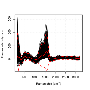
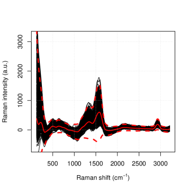
Figure 2: For the healthy (left) and tumoral (right) data set we report the smoothed spectra (black solid lines), the average spectra (red solid lines), and the extreme curves computed by adding to and subtracting from the average Raman intensity three times the standard deviation (red dashed lines) labeling the decision surfaces.

2.4 Two statistical approaches

We will propose two different models, one based on the PCA analysis and one based on the computation of $\ell^{2}$ distance. The spectra are split into test and training sets, the first used to tune simultaneously the parameters of both the models here proposed, the second to validate them. As aforementioned, we deal with a binary target variable $W$, whose outcomes 1 and 0 correspond to tumoral and healthy DNA molecules respectively.

2.4.1 The local method: PCA analysis and logistic regression

Borrowing the notation from [21, Chapter 1 and Paragraph 8.2.1], any single spectrum is represented as a column vector $x\in\mathbb{R}^{p}$. By collecting the $N$ row vectors $x^{\dagger}$, where ${\dagger}$ denotes transpositions, we construct the $N\times p$ matrix $\mathbf{X}$ which represents the entire data set. The $j$–th column of $\mathbf{X}$ is the collection of the $N$ observations of the $j$–th variable, namely, the intensity corresponding to the $j$–th value of the Raman shift.

Thus, we produce the $N\times p$ matrix $\mathbf{Y}$ by centering $\mathbf{X}$ with respect to the columns (i.e., the Raman shift). More in details, each entry $y_{ij}$ of $\mathbf{Y}$ is computed by subtracting to each entry $x_{ij}$ of $\mathbf{X}$ the sample mean computed along the elements corresponding to the same Raman shift, that is to say by setting

$$y_{ij}=x_{ij}-\frac{1}{N}\sum_{s=1}^{N}x_{sj}$$ (2.1)

for any $i=1,\dots,N$ and $j=1,\dots,p$. A principal components analysis is then obtained by the eigendecomposition of the empirical covariance matrix $\textbf{Y}^{\dagger}\textbf{Y}$ (see, for example, [22]). The so–called principal components directions $v_{1},\dots,v_{p}\in\mathbb{R}^{p}$ are computed and, as usual, we call $i$–th principal component loadings the $p$ elements of the column vector $v_{i}$. The projection $\mathbf{z}_{i}=\mathbf{Y}v_{i}\in\mathbb{R}^{N}$ is called $i$–th principal component of the data $\mathbf{Y}$. The variance of each principal component (PC) is given by the corresponding eigenvalue and it concentrates on the first $m$ principal components, allowing us to neglect in the next step all the other $p-m$ components.

The selected first $m$ principal components $z_{1},\dots,z_{m}$ are thus interpolated to build a logistic regression model to estimate the probability mass function of the binary target variable $W$ by

$$\textup{Pr}(W=1|z_{1},\dots,z_{m})=\frac{e^{\beta_{0}+\sum_{i=1}^{m}\beta_{i}z_{i}}}{1+e^{\beta_{0}+\sum_{i=1}^{m}\beta_{i}z_{i}}}\;\;\textup{ and }\;\;\textup{Pr}(W=0|z_{1},\dots,z_{m})=\frac{1}{1+e^{\beta_{0}+\sum_{i=1}^{m}\beta_{i}z_{i}}},$$ (2.2)

where $\beta_{i}\in\mathbb{R}$ for $i=0,\dots,m$. In this case, we consider an optimization parameter $\lambda\in[0,1]$ such that we associate the outcome for the binary variable $W=1$ to each set of components $z_{1},\dots,z_{m}$ if $\textup{Pr}(W=1|z_{1},\dots,z_{m})\geq\lambda$ and $W=0$ otherwise. This method is referred as “local” since the PCA analysis selects a subset of spectral indices to be the most relevant within the subsequent regression.

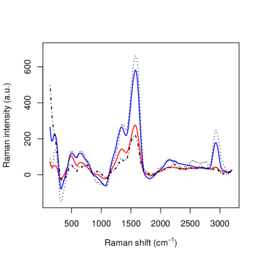
Figure 3: The red and the blue solid lines are, respectively, the average spectrum of the healthy and the tumoral data set. The point–dashed and the dashed lines report, respectively, one healthy and tumoral pre–processed spectrum. For the healthy spectrum $\textup{d}_{t}=14.9\times 10^{6}$ and $\textup{d}_{h}=4.7\times 10^{6}$. For the tumoral spectrum $\textup{d}_{t}=2.8\times 10^{6}$ and $\textup{d}_{h}=16.6\times 10^{6}$.

2.5 The global method: geometric analysis

The second proposed strategy aims to distinguish spectra coming from the healthy and tumoral data set following their geometric features.

After splitting the dataset into training and test sets, the training set is used to produce the healthy and the tumoral average spectra, represented by the column vectors $h$ and $t$ of $\mathbb{R}^{p}$. Thus, for each spectrum belonging to the test set represented by the $i$–th row of the data matrix $\mathbf{X}$, we compute the $\ell^{2}$ distances

$$\textup{d}_{h}(i)=\sum_{s=1}^{p}|x_{is}-h_{s}|^{2}\;\;\textup{ and }\;\;\textup{d}_{t}(i)=\sum_{s=1}^{p}|x_{is}-t_{s}|^{2}.$$ (2.3)

so that each spectrum can be classified by setting the following outcome binary function

$$g_{\textup{out}}(i)=\mathbbm{1}\{\tau\textup{d}_{t}(i)\leq(1-\tau)\textup{d}_{h}(i)\},$$ (2.4)

where $\tau\in[0,1]$ is an optimization parameter. As above, the outcome is equal to $0$ if the spectrum is identified as coming from healthy DNA molecules and equal to $1$ otherwise. This method is referred as “global” since the $\ell^{2}$ distance is computed over the complete set of spectral data.

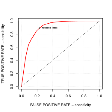
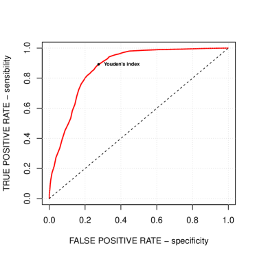
Figure 4: ROC curves for the local (left panel) and the global (right panel) methods. The markers put in evidence the corresponding Youden’s indices.

Figure 5: Left: the four solid lines reports the loadings associated to the first four principal components (blue first, brown second, green third, and yellow fourth); the dashed black lines is the intensity, i.e., the square root of the sum of the squares, of the loadings of the first four components. Right: percentage of variance as function of the principal component index.

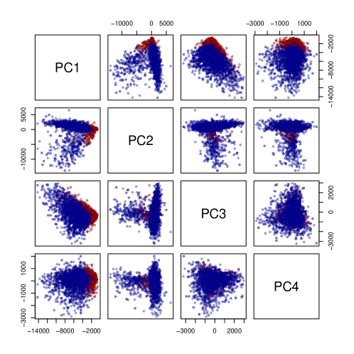
Figure 6: Projections on the coordinate planes of the distribution of the first four principal components on the coordinate planes.

Method	optimal tuning parameter	Area Under the Curve
local	$\lambda=0.46$	0.899
global	$\tau=0.34$	0.871

Table 2.1: Optimal tuning parameters and AUC for both the methods.

Principal component	Standard deviation	Proportion of Variance	Cumulative Proportion
PC1	5157.11860	0.78068	0.78068
PC2	2311.49810	0.15684	0.93752
PC3	866.34106	0.02203	0.95955
PC4	581.91444	0.00994	0.96949
PC5	496.66847	0.00724	0.97673
PC6	405.79667	0.00483	0.98156
PC7	327.32049	0.00314	0.98471
PC8	284.63234	0.00238	0.98708

Table 2.2: Variance analysis (first 8 principal components).

3 Results and discussion

We estimate first the tuning parameters $\lambda$ and $\tau$ by means of a $10$–fold cross–validation procedure, a popular method used to evaluate predictive models over a limited amount of sampled data (see [23, Ch. 7]).

The original sample is randomly partitioned into 10 equally sized subsamples. A subsample is kept as test set, while the other nine ones are used as training data. Then the accuracy of both the methods are evaluated, while the cross–validation process is repeated 10 times, paying attention to use each round a different subsample as test group. The 10 results are then averaged to compute a single estimation. The advantage of this validation strategy is that all observations are used at the same time for both training and testing and each observation is used for testing exactly once.

The accuracy of the choice of the tuning parameters is evaluated by means of the so–called Youden’s $J$ statistic, or – simpler, Youden’s index, given by the formula

$$\text{Youden's index}=\text{sensitivity}+\text{specificity}-1,$$ (3.5)

where sensitivity and specificity are the true and false positive rates respectively. Figure 4 explores the trade–off between specificity and sensitivity by means of the corresponding ROC curve, while Table 2.1 presents for both the models the choice of the optimal tuning parameters, corresponding to the maximal Youden’s indices, and the Area Under the Curve (AUC) value, measuring the two–dimensional area under the ROC curve and providing thus an aggregate measure of the performance across all possible choices of the tuning parameters (see, for example, [24]).

As shown in Table 2.1, both $\lambda$ and $\tau$ are smaller than $1/2$, which is the exact balance of the healthy and tumoral subsets. However, it matches our goals since these values of the tuning parameters reduce the amount of false negatives (i.e., not detecting tumoral samples) paying the price of a larger amount of false positives (i.e., misclassifying healthy samples), which seems to be the fairest choice.

Concerning the PCA analysis, as shown in Table 2.2 (see the right panel in figure 5), $97.0\%$ circa of the variance concentrates on the first $m=4$ principal components. Furthermore, figure 6 shows a strong separation between the third and fourth principal component. Thus, from now on, only the first 4 principal components are selected. Also, each discarded component is characterized by a proportion of variance sensibly smaller than $1\%$ (see again Table 2.2).

$i$	Estimate	Standard Deviation
0	-6.6094526	0.2424116
1	-0.0014903	0.0000540
2	-0.0002585	0.0000440
3	-0.0020081	0.0001042
4	-0.0007470	0.0001154

Table 3.3: Estimates of $\beta_{i}$ and corresponding errors.

The left panel in figure 5 collects the loadings, that is, the coefficients of the linear combinations of the original variables defining the principal components, related to the first four PC’s, and, thus, provide a measure for the contribution of each observable to the main components. The solid lines are concerned with the first four PC’s separately, while the dashed black line represents the associated intensity, that is, the $\ell^{2}$–norm associated to the loadings of the considered PC’s. The three main peaks appearing in the panel correspond to wavenumber 230 cm^-1, $1550$ cm^-1, and 2930 cm^-1. The first one is related to the Ag–N stretching vibration mode. The second one is contributed both by the overlapping of C–C and C–N stretching vibrations involving the aromatic rings of the DNA bases, and the so–called “cathedral peaks", deriving from the formation of a carboneous layer due to the photo–decomposition of the DNA at the silver surface upon laser irradiation. The last one is linked to the vibrations of the CH–group.

The estimates for the coefficients $\beta_{i}$, $i=0,\ldots,4$ obtained by the logistic regression are collected in Table 3.3. Recall that, in this case, the optimization parameter $\lambda\in[0,1]$ is defined such that $W=1$ for each $z_{1},\dots,z_{4}$ if $\textup{Pr}(W=1|z_{1},\dots,z_{4})\geq\lambda$, otherwise $W=0$.

Population (col.) vs. Prediction (row)	Positive (%)	Negative (%)
Positive (%)	44.6/44.6	11.6/13.8
Negative (%)	5.3/5.4	38.4/36.2

Table 3.4: Confusion matrix (local method / global method).

We evaluate, now, the accuracy of the proposed methods by means of the two confusion matrices in Table 3.4 (see, again, [24]) computed by averaging true positives (TP), true negatives (TN), false positives (FP), and false negatives (FN) over all the possible choices of the training and the test set of data. We use the values collected in Tables 3.4 to calculate, for both the methods, the so–called Cohen’s $\kappa$ statistic, which takes values in $[-1,+1]$ and measures the agreement between two classifiers and can also be used to assess the performance of a classification model, given by the formula (in the binary case)

$$\kappa=\frac{2\left(\text{TP}\times\text{TN}-\text{FP}\times\text{FN}\right)}{\left(\text{TP}+\text{FP}\right)\left(\text{FP}+\text{TN}\right)+\left(\text{TP}+\text{FN}\right)\left(\text{FN}+\text{TN}\right)},$$ (3.6)

see, for example, [25]. For the first method, we obtain $\kappa_{\text{local}}=0.66$, while for the second $\kappa_{\text{global}}=0.62$. Both values put in evidence a good agreement and accuracy in predictions for both the methods.

Now, we aim to evaluate the performance of the combination of the two methods, with the purpose of improving predictions and, at the same time, reducing the variance in the predictions and, thus, enhancing their stability. Table 3.5 compares the reliability of the predictions of the two models, averaging over the outcomes of the 10–fold cross–validation performed for the optimal tuning parameters. It is important to remark that when the outcomes for both models are either 0 (TN or FN) or 1 (TP or FP), the amount of correct prediction is $92.2\%$ (negative predictive value) and $81\%$ (positive predictive value), respectively. Furthermore the total proportion of wrong negative outcomes is $2.9\%$.

Local (row) vs. Global (col.)	TP(%)	FP(%)	FN(%)	TN(%)
TP(%)	42.1		2.5
FP(%)		9.7		1.9
FN(%)	2.5		2.9
TN(%)		4.1		34.3

Table 3.5: Performance of the outcomes for the joint methods. Empty cells correspond to impossible combinations of outcomes.

Table 3.6 investigates on the accuracy of the predictions. Even if $11\%$ of the predictions are at odds, and thus they should be directly marked as unreliable, $86\%$ (joint accuracy) predictions are valid when both agree.

Local (row) vs. Global (col.)	correct predictions (%)	wrong predictions (%)
correct predictions (%)	76.4	6.6
wrong predictions (%)	4.4	12.6

Table 3.6: Correct vs. wrong predictions (joint models).

4 Conclusions

Raman spectra of tumoral and healthy genomic DNA have been collected by analyzing aqueous DNA droplets deposited onto silver–coated silicon nanowires. We used, respectively, the human melanoma cell line SK–MEL–28 and the human immortalized keratinocyte HaCaT as tumoral and healthy samples.

Pre–processed spectra were analyzed by means of two different techniques: a PCA based algorithm powered with linear regression and a purely geometric algorithm were devised to predict the tumoral or healthy origin of each spectra. Both algorithms achieve very high accuracy, close to $90$%. We also checked accuracy by means of the Cohen’s $\kappa$ statistic and for both algorithms we found very good values of the Cohen’s $\kappa$ index – larger than $0.6$.

On one hand the PCA approach, rather standard in analyzing Raman measurements, aims at reducing the data set through the analysis of the covariance matrix. On the other hand, the geometric method that we implemented in this paper looks at the whole set of data and is based on the simple computation of the $\ell^{2}$ distance between spectra. The fact that both methods work nicely in discriminating healthy and tumoral molecules is a strong sign of the robustness of the indications provided by the Raman measurements.

In conclusion, we developed a detailed statistical analysis which proves that SERS measurements can be successfully used for efficient and fast cancer diagnostic applications. In particular, our innovative classification approach allows a rapid and unexpansive discrimination between healthy and tumoral genomic DNA, and represents a powerful alternative to the more complex and expensive DNA sequencing. Moreover, the proposed algorithms, implemented in commercial benchtop Raman spectrophotometers, could open the way to a completely automatic diagnostic analysis.

Acknowledgements

The research activity is funded by Regione Lazio within the project DIANA, “DIAgnostic potential of disorder: development of an innovative NAnostructured platform for rapid, label–free and low–cost analysis of genomic DNA”, POR FESR Lazio 2014 – 2020, Progetti Gruppi di ricerca call 2020, A0375-2020-36589, CUP B85F21001240002.

A.C. acknowledges the support of the Italian Minister of Foreign Affairs and International Collaboration (MAECI) under the Joint research project “Scalable nano–plasmonic platform for differentiation and drug response monitoring of organtropic metastatic cancer cells” (US19GR07).

References

- [1] K. Kong, C. Kendall, N. Stone, and I. Notingher. Raman spectroscopy for medical diagnostics — From in–vitro biofluid assays to in–vivo cancer detection. Advanced Drug Delivery Reviews, 89:121–134, 2015.
- [2] Z. Liu, S. Parida, R. Prasad, R. Pandeya, D. Sharma, and I. Barman. Vibrational spectroscopy for decoding cancer microbiota interactions: Current evidence and future perspective. Seminars in Cancer Biology, 2021.
- [3] V. Mussi, M. Ledda, D. Polese, L. Maiolo, D. Paria, I. Barman, M.G. Lolli, A. Lisi, and A. Convertino. Silver–coated silicon nanowire platform discriminates genomic DNA from normal and malignant human epithelial cells using label–free raman spctroscopy. Material Science & Engineering C, 122:111951, 2021.
- [4] Z. Movasaghi, S. Rehman, and I.U. Rehman. Raman Spectroscopy of Biological Tissues. Applied Spectroscopy Reviews, 42:493–541, 2007.
- [5] A.C.S. Talari, Z. Movasaghi, S. Rehman, and I.U. Rehman. Raman Spectroscopy of Biological Tissues. Applied Spectroscopy Reviews, 50:46–111, 2015.
- [6] R. Petry, M. Schmitt, and J. Popp. Raman spectroscopy – a prospective tool in the life sciences. Chemphyschem: a European journal of chemical physics and physical chemistry, 4:14–30, 2003.
- [7] M. Fleischmann, P.J. Hendra, and A.J. McQuillan. Raman spectra of pyridine adsorbed at a silver electrode. Chemical Physics Letters, 26:163–166, 1974.
- [8] C.L. Haynes, A.D. McFarland, and R.P. Van Duyne. Surface–Enhanced Raman Spectroscopy. Analytical Chemistry, 77:338A–346A, 2005.
- [9] P.L. Stiles, J.A. Dieringer, N.C. Shah, and R.P. Van Duyne. Surface–Enhanced Raman Spectroscopy. Annual Review of Analytical Chemistry, 1:601–626, 2008.
- [10] A. Convertino, V. Mussi, and L. Maiolo. Disordered array of Au covered Silicon nanowires for SERS biosensing combined with electrochemical detection. Scientific Reports, 6:25099, 2016.
- [11] A. Convertino, V. Mussi, L. Maiolo, M. Ledda, M.G. Lolli, F.A. Bovino, G. Fortunato, M. Rocchia, and A. Lisi. Array of disordered silicon nanowires coated by a gold film for combined NIR photothermal treatment of cancer cells and Raman monitoring of the process evolution. Nanotechnology, 29:415102, 2018.
- [12] B. Zhang, H. Wang, L. Lu, K. Ai, G. Zhang, and X. Cheng. Large–Area Silver–Coated Silicon Nanowire Arrays for Molecular Sensing Using Surface–Enhanced Raman Spectroscopy. Advanced functional materials, 18:2348–2355, 2008.
- [13] E. Galopin, J. Barbillat, Y. Coffinier, S. Szunerits, G. Patriarche, and R. Boukherroub. Silicon Nanowires coated with Silver Nanostructures as Ultrasensitive Interfaces for Surface–Enhanced Raman Spectroscopy. ACS Appl. Mater. Interfaces, 7:1396–1403, 2009.
- [14] M.-L. Zhang, X. Fan, H.-W. Zhou, M.-W. Shao, J.A. Zapien, N.-B. Wong, and S.-T. Lee. A High–Efficiency Surface–Enhanced Raman Scattering Substrate Based on Silicon Nanowires Array Decorated with Silver Nanoparticles. J. Phys. Chem. C, 114:1969–1975, 2010.
- [15] D. Paria, A. Convertino, V. Mussi, L. Maiolo, and I. Barman. Silver–Coated Disordered Silicon Nanowires Provide Highly Sensitive Label–Free Glycated Albumin Detection through Molecular Trapping and Plasmonic Hotspot Formation. Advanced healthcare materials, 10:2001110, 2021.
- [16] M.S. Schmidt, J. Hübner, and A. Boisen. Large Area Fabrication of Leaning Silicon Nanopillars for Surface Enhanced Raman Spectroscopy. Advanced materials, 24:OP11–OP18, 2012.
- [17] C.E.M. Weber, C. Luo, A. Hotz-Wagenblatt, A. Gardyan, T. Kordaß, T. Holland-Letz, Wi. Osen, and S.B. Eichmüller. miR–339–3p Is a Tumor Suppressor in Melanoma. Cancer research, 76:3562–3571, 2016.
- [18] M.R. Stratton, P.J. Campbell, and P.A. Futreal. The cancer genome. Nature, 458:719–724, 2009.
- [19] A. Savitzky and M.J.E. Golay. Smoothing and Differentiation of Data by Simplified LeastSquares Procedures. Anal. Chem., 36:1627–1639, 1964.
- [20] B. Zimmermann and A. Kohler. Optimizing Savitzky–Golay parameters for improving spectral resolution and quantification in infrared spectroscopy. Appl. Spectrosc., 67(8):892–902, 2013.
- [21] T. Hastie, R. Tibshirani, and M. Wainwright. Statistical Learning with Sparsity: The Lasso and Generalizations. CRC Press, Routledge, 2015.
- [22] J.E. Jackson. A User’s Guide to Principal Components. Wiley, 1991.
- [23] T. Hastie, R. Tibshirani, and J. Friedman. The elements of statistical learning. Springer, 2009.
- [24] T. Fawcett. An introduction to ROC analysis. Pattern Recognition Letters, 28:861–874, 2006.
- [25] D. Chicco, M.J. Warrensand, and G. Jurman. The Matthews correlation coefficient (MCC) is more informative than Cohen’s Kappa and Brier score in binary classification assessment. Access, 9:78368–78381, 2021.